Embed Size (px)
Citation preview

FACULDADE DE ENGENHARIA DA UNIVERSIDADE DO PORTO
Neural Encoding Models in NaturalVision
Nuno Pedro Pinto Albuquerque Sousa
Mestrado Integrado em Bioengenharia
Orientador: João Manuel R. S. Tavares (FEUP/DEMec)
September 20, 2013


Neural Encoding Models in Natural Vision
Nuno Pedro Pinto Albuquerque Sousa
Mestrado Integrado em Bioengenharia
September 20, 2013


Abstract
From the existing medical imagiology tools, it has been progressively more possible to correctlyshow the association between cognitive sensorial processes and zones in the brain. Recently, theacquisition of Functional Magnetic Resonance Imaging (fMRI) has enabled the partial reconstruc-tion of the the images that were being exhibited to the subject in experiments where visual stimuliare presented while the neural activity is recorded - which is to say, technologies are emerging thatwill allow to extract the visual signals from the brain.
The effort to transform fMRI signals into the original stimulus relies heavily on the construc-tion of decoding models of neural and neuronal brain activity. This work presents a study on thefunctional characteristics of neurons, in particular from the primary visual motor cortex, and thesubsequent implementation of models which attempt to predict the response of neurons of thearea to natural visual stimuli. The data used comes from the Neural Prediction Challenge and ispresented in a ’contest’ environment where users are encouraged to test their results in a blindresponse test. This data was provided by Gallant Labs from University of California Berkley.
The implementation of the state of the art algorithms and models was performed, and someinnovations, notably the use of KNN Classifiers for "Fire or not" classification, and NARX neuralnetworks to model non-ideal characteristics of neurons were attempted. A massive neural networkbased aproach was also atempted but failed to reach fruition because of technical considerations.
The selected improvements can marginally increase performance from the current state ofthe art by about 2%, which is a relative success considering that in the past 8 years the fieldonly saw a 10% improvement in prediction accuracy. A speedup of 5× can also be reported byimplementing some of the critical computations on the GPU as well as reduction of 10× in acritical part of the state of the art algorithm - considering the overhead and other functions thistranslates into a practical up to 1200% speed improvement, with the approximate same results(equal when converted to single precising floating point).
i

ii

Acknowledgements
Firstly a word of praise to the resarchers at Gallant Labs which so kindly provide access to thepublic of rather rare and so high quality material. I would like to thank specially my Supervisor,Professor João Tavares, for the disponibility and guidance, as well as his high quality scientificlibrary.
A word of aknowledgment to the great work of Professor Gallant, and Dr. Neselaris and allthose which make science fiction possible through their innovative resarch into the vision pro-cesses into the brain.
To Professor Aurélio Campilho, for teaching me the arts of classifiers and machine learning,on which this piece of work mostly settles.
A special thanks to my family for their support during the late hours of work and the earlyfrustrations in particular to my mother, and to my friends, which were always there to help metake my mind off work whenever it became too much. A special thanks to Michael Oliver forproviding his code and methods for the improvement of my own work.
Nuno Pedro Pinto Albuquerque Sousa
iii

iv

“One man’s ’magic’ is another man’s engineering.’Supernatural’ is a null word..”
Robert A. Heinlein
v

vi

Contents
1 Introduction 11.1 Motivation . . . . . . . . . . . . . . . . . . . . . . . . . . . . . . . . . . . . . . 21.2 Applications . . . . . . . . . . . . . . . . . . . . . . . . . . . . . . . . . . . . . 31.3 Objectives . . . . . . . . . . . . . . . . . . . . . . . . . . . . . . . . . . . . . . 41.4 Organization . . . . . . . . . . . . . . . . . . . . . . . . . . . . . . . . . . . . . 41.5 Integration Into Scientific Endeavor . . . . . . . . . . . . . . . . . . . . . . . . 5
2 Neuron 72.1 The Neuron . . . . . . . . . . . . . . . . . . . . . . . . . . . . . . . . . . . . . 7
2.1.1 Synapse . . . . . . . . . . . . . . . . . . . . . . . . . . . . . . . . . . . 82.2 Neuron Firing . . . . . . . . . . . . . . . . . . . . . . . . . . . . . . . . . . . . 9
2.2.1 Action Potential . . . . . . . . . . . . . . . . . . . . . . . . . . . . . . 102.2.2 Synaptic Transmission . . . . . . . . . . . . . . . . . . . . . . . . . . . 12
2.3 Firing rates and Impulse Trains . . . . . . . . . . . . . . . . . . . . . . . . . . . 152.3.1 Fire rate nomenclature . . . . . . . . . . . . . . . . . . . . . . . . . . . 162.3.2 From Spike Trains to Firing Rates . . . . . . . . . . . . . . . . . . . . . 16
2.4 Simple Neuron Models . . . . . . . . . . . . . . . . . . . . . . . . . . . . . . . 19
3 The Visual Cortex and Vision 213.1 The eye . . . . . . . . . . . . . . . . . . . . . . . . . . . . . . . . . . . . . . . 21
3.1.1 Global Anatomy . . . . . . . . . . . . . . . . . . . . . . . . . . . . . . 213.1.2 Retina . . . . . . . . . . . . . . . . . . . . . . . . . . . . . . . . . . . . 223.1.3 Implications on Neural coding . . . . . . . . . . . . . . . . . . . . . . . 27
3.2 From the Optic Nerve to the Visual Cortex . . . . . . . . . . . . . . . . . . . . . 273.2.1 The Visual Cortex . . . . . . . . . . . . . . . . . . . . . . . . . . . . . 28
3.3 The V1 Neuron . . . . . . . . . . . . . . . . . . . . . . . . . . . . . . . . . . . 28
4 STRF Methods 314.1 STRF . . . . . . . . . . . . . . . . . . . . . . . . . . . . . . . . . . . . . . . . 31
4.1.1 LNP Model . . . . . . . . . . . . . . . . . . . . . . . . . . . . . . . . . 324.2 Image Domain . . . . . . . . . . . . . . . . . . . . . . . . . . . . . . . . . . . 33
4.2.1 STA and STC . . . . . . . . . . . . . . . . . . . . . . . . . . . . . . . . 344.3 Gabor Wavelet Transform . . . . . . . . . . . . . . . . . . . . . . . . . . . . . . 364.4 Optimization Algorithms . . . . . . . . . . . . . . . . . . . . . . . . . . . . . . 38
4.4.1 Gradient Descent . . . . . . . . . . . . . . . . . . . . . . . . . . . . . . 384.4.2 Coordinated Gradient Descent . . . . . . . . . . . . . . . . . . . . . . . 424.4.3 LARS . . . . . . . . . . . . . . . . . . . . . . . . . . . . . . . . . . . . 424.4.4 Thresholded Gradient Descent . . . . . . . . . . . . . . . . . . . . . . . 43
vii

CONTENTS
4.5 Other Methods . . . . . . . . . . . . . . . . . . . . . . . . . . . . . . . . . . . 434.5.1 KNNC . . . . . . . . . . . . . . . . . . . . . . . . . . . . . . . . . . . 434.5.2 Adaptative Threshold Fitting . . . . . . . . . . . . . . . . . . . . . . . . 444.5.3 Resampling . . . . . . . . . . . . . . . . . . . . . . . . . . . . . . . . . 454.5.4 NARX Networks . . . . . . . . . . . . . . . . . . . . . . . . . . . . . . 45
4.6 Computational Implementation . . . . . . . . . . . . . . . . . . . . . . . . . . . 464.6.1 Distributed Computing . . . . . . . . . . . . . . . . . . . . . . . . . . . 474.6.2 GPU Optimization . . . . . . . . . . . . . . . . . . . . . . . . . . . . . 47
5 Results 515.1 Measurement of Performance . . . . . . . . . . . . . . . . . . . . . . . . . . . . 515.2 Parameter Sweep . . . . . . . . . . . . . . . . . . . . . . . . . . . . . . . . . . 52
5.2.1 Available Methods . . . . . . . . . . . . . . . . . . . . . . . . . . . . . 525.2.2 NARXdelays . . . . . . . . . . . . . . . . . . . . . . . . . . . . . . . . 535.2.3 Thresholds . . . . . . . . . . . . . . . . . . . . . . . . . . . . . . . . . 535.2.4 Gabor Parameters . . . . . . . . . . . . . . . . . . . . . . . . . . . . . . 545.2.5 Overall Sweeping Interpolation . . . . . . . . . . . . . . . . . . . . . . 54
5.3 Results . . . . . . . . . . . . . . . . . . . . . . . . . . . . . . . . . . . . . . . . 545.3.1 Wavelet Transform . . . . . . . . . . . . . . . . . . . . . . . . . . . . . 555.3.2 Adaptive Threshold . . . . . . . . . . . . . . . . . . . . . . . . . . . . . 555.3.3 Legacy STA / STC . . . . . . . . . . . . . . . . . . . . . . . . . . . . . 555.3.4 Gradient Descent . . . . . . . . . . . . . . . . . . . . . . . . . . . . . . 585.3.5 Coordinated Gradient Descent . . . . . . . . . . . . . . . . . . . . . . . 585.3.6 LARS . . . . . . . . . . . . . . . . . . . . . . . . . . . . . . . . . . . . 585.3.7 Thresholded Gradient Descent . . . . . . . . . . . . . . . . . . . . . . . 605.3.8 KNN . . . . . . . . . . . . . . . . . . . . . . . . . . . . . . . . . . . . 61
5.4 Final Results . . . . . . . . . . . . . . . . . . . . . . . . . . . . . . . . . . . . 62
6 Conclusions and Future Work 656.1 Additional Work . . . . . . . . . . . . . . . . . . . . . . . . . . . . . . . . . . 65
6.1.1 Further Computational Optimization . . . . . . . . . . . . . . . . . . . . 666.2 Current State of Neural Coding . . . . . . . . . . . . . . . . . . . . . . . . . . . 666.3 Future Improvement . . . . . . . . . . . . . . . . . . . . . . . . . . . . . . . . 67
A Matlab Code Listing 69A.1 Main algorithm - unicase . . . . . . . . . . . . . . . . . . . . . . . . . . . . . . 69A.2 Speedup - Profiler . . . . . . . . . . . . . . . . . . . . . . . . . . . . . . . . . . 79
References 85
viii

List of Figures
1.1 These tests were performed on two subjects. In the upper line the exhibited stimuliare shown, and through a decoding model and fMRI mapping, the reserchers fromATR Computational Neurostudies Institute were able to reconstruct the image asshown in the following lines. In the last line the average of the various samplesis shown, and can be confirmed to contain the characteristics (leter discerning andaspect) of the original. [MUY+08]. . . . . . . . . . . . . . . . . . . . . . . . . . 2
1.2 Reconstruction of the clip from the brain of the subject through the utilization offMRI. This experiment gained notoriety because through fMRI data acquisition,centered in the occipital lobe ( where the visual cortex is located) with high tem-poral resolution, was possible to observe what the human mind sees. The methodfor reconstruction lies in an extensive sample database for the subject, with hun-dreds of hours of film and response. The neural responses were processed intoresponses to 3D filtering (2D images + time), and then the observed response’schannels (filter responses) were correlated to each of the databank’s responses, thetop 100 candidates were averaged to show the predicted image [NVN+11]. . . . 3
2.1 There is a relative myriad of types of neuron, the shown shapes are but a subset ofthe variety found in a complex being such an highly evolved mammal, which pos-sesses very specific neurons for different functions, as well as neuron like cells inthe heart, in the sensory systems, which together make for a wealth of types.[Stu08] 8
2.2 As shown, neurons can communicate and propagate their signals with one an-other both through synaptic clefts using chemical neurotransmitters, and the directconnection of denditric trees. In the above image when the signals reaches thecluster of the four neurons they all fire. Given that each neuron has one and onlyone axon this allows for the dendritic trees to be the effectors of the one-to-manycommunication in neural networks.[Stu08] . . . . . . . . . . . . . . . . . . . . . 9
2.3 The action potential (A -right) and the synaptic junction or cleft (B - right). A -This is a typical curve of membrane potential across time upon the firing of a neu-ron. The rest potential is broken and the membrane polarizes (often unto positivevalues) by the entry of Sodium through Na+ Channels, followed by the action ofNa+/K+ pumps which restore the balance, and with the reentry of chlorine a stateof hyper polarization is achieved, which marks the end of the refractory period.The potential stabilizes again into the resting potential and the neuron can fireagain. B - The synaptic cleft is a privileged medium for the transaction of neuro-transmitters between the incoming neuron and the outgoing one. In this cleft theemitting neuron releases vesicles filled with neurotransmitters such as: adrenalin,seratonin, Acetylcholin, dopamine among many [Cle96]. [DA01] . . . . . . . . . 11
ix
LIST OF FIGURES
2.4 The meachanism of propagation relies on the reinforcement effect of the varioussodium channels. Being voltage gated, when they sense the change in potentialinside the cell they contribute to the effect by opening up themselves thus creatinga new focus of entry. Thus they progressivly activate each other until the potentialreaches the synaptic cleft. [act] . . . . . . . . . . . . . . . . . . . . . . . . . . . 12
2.5 Types of measurement of action potential. Top - measurement on the soma, withgreater detail near the baseline which conveys some info. The dashed line standsfor clipping, to better show the lower part of the curves, for the potential is similarto the bottom measurment. Middle - Extracellular recording on the medium. Thepotential is about 1000× smaller in amplitude yet can be detected. Bottom - Mea-surement by contact with axon, full scale potential, and greater ease of usage thanmeasuring in the soma, as some axons are very long and easy to connect with innerve tissue. [DA01] . . . . . . . . . . . . . . . . . . . . . . . . . . . . . . . . 13
2.6 Original stimulus and processing to fire rate. From top to bottom : 1 - Originalsignal for the neuron 206B from the Neural Prediction Challenge, not a number(NaN) values removed. 2,3,4 - Conversion to fire rate through convolution witha box window of specified size. Note the smoothness created, which obstructsthe original details, but at the same time is easier to aproximate by Optimizationalgorithms. 5 - Convolution with a Gaussian Kernel , results in more fidelity thanthe same size box window and is arguably of the same smoothness (Notice thepeaks at t=12). Original Image . . . . . . . . . . . . . . . . . . . . . . . . . . . 18
3.1 Anatomy of the eye, seen from a sagital cut.[WR77] . . . . . . . . . . . . . . . . 22
3.2 Typical behaviour of ganglion cells to light on their receptive fields. This sort ofprocessing is a little bit like edge detection, and ist very atuned to motion. Notethat the light is pulsated in order to constantly provoke response (a steady lighteven in the right pattern fails to be effective at provoking high fire rates[Wik13b]. 25
3.3 Organization of the retina. Light propagates from bottom to top. Neural spikestravel top to bottom. The various layers are represented. Simplified mechanism ofaction: the spike is generated in the cones or rods, is grouped and transmitted tothe bipolar cells, suffering lateral processing from horizontal cells. In then travelsto ganglions, either directly or through amacrine cells (which also introduce lateralprocessing), and from the ganglion goes into the optic nerve.[ret] . . . . . . . . 26
3.4 In this figure it’s possible to see what the various nerve bundles carry in terms ofinformation from the visual field. Notice the nerve crossover at the optic chiasm,where the nasal looking parts of the retina are sent to complement the vision fromthe periphery of the other side.[Fix94] . . . . . . . . . . . . . . . . . . . . . . . 28
3.5 Various areas responsible for the processing of vision. Not labeled: above V3A inpurple - V7 zone[Log99] . . . . . . . . . . . . . . . . . . . . . . . . . . . . . . 29
3.6 Study on the preferred orientations of the response of V1 Neurons performed inmacaques. It was determined that orientations varied 3o to 10o , and that therewas an organzation in the cortex, with similar orientations close together. Theprobing needle was displaced along an axial cut of the cortex and the preferentialorientation was determined by showing various orientations of flickering bars andfinding the one with maximum response. It was also found that a similar patternemerges with depth into the cortex, but to a lighter extent. Modified from [HW74] 29
x
LIST OF FIGURES
4.1 The LNP Model - The linear combination of responses of the stimulus to a filterare then passed through a non-linearity function and then the spikes occur ran-domly following a Poisson distribution whose parameters are constrained by theinstantaneous firing rate. The diagram shows for simple neurons (A) of the V1cortex there is only one prefered direction and spatial frequency. For complexneurons often the combination of several filters is needed to approximate their re-sponse (B). In the bottom the STA and STC are shown to a stimulus of black andwhite bars presented to the subject. The idea is to create moving windows. By av-eraging the resulting windows STA is created, by estimating the covariance STCis calculated .[RSMS05] . . . . . . . . . . . . . . . . . . . . . . . . . . . . . . 33
4.2 Typical frames from the stimulus. Top: This is the "high quality version" at 136×136 resolution. These are the images shown to the subject primates in their nativeresolution. Clip size varies from 8000 to 20000 frames - up to 320s. Bottom : Lowresolution down-sampled segment of the region of interest - determined by STA . 34
4.3 In this figure it’s possible to see in more detail the computation resulting in anSTA. [Wik13c] . . . . . . . . . . . . . . . . . . . . . . . . . . . . . . . . . . . 35
4.4 Top Row: STA results for TSTA = 4 for neuron 206B. RTA and RTC mean thesame thing as STA and STC but are used when instead of a spike train we usea PSTH to calculate - Response Triggered Average instead of Spike TriggeredAverage. For the various delays it’s possible to see a gabor like structure forming,with low spatial frequency - This STA can be used to generate predictions byconvolving it with the stimuli (though with very low quality). Bottom two rows:STC Projections : STC is a matrix whose orthogonal projection STC1 and STC2are used as values for a latter stage of optimization and can be used for creatingpredictions by linear combination.The visualization of the projections elucidatesas to the direction vectors which most affect the response. . . . . . . . . . . . . 36
4.5 3D visualization of a Gabor Filter - This is a single specimen, a filter bank is madeout of thousands like these, varying in orientation, placement, frequency amongstother parameters. This filter is multiplied together with a motion function by thevideo to generate a single channel, a signal varying over time. . . . . . . . . . . 37
4.6 A single gabor 3D filter, with a temporal size of 9. From left to right temporalindexes : -4 to 4. The Gabor filters have a sensitivity to changing features. Thisparticular one has a short temporal velocity and a low spatial frequency. This is achannel representing the half wave rectified real part |Re(g)|+ . . . . . . . . . . 38
4.7 Gradient Descent - here is shown a simple gradient descent on two dimensionalfeature space. Our actual case is highly dimensional but it shows the principle ofprogressing in favour of the gradient (or against it if we consider the gradient tobe positive when rising) [Wik13a] . . . . . . . . . . . . . . . . . . . . . . . . . 40
4.8 KNN classification - For a new sample the class of the k closest neighbours ofthat sample determines the classification, majority rules. From http://www.statistics4u.com/fundstat_eng/cc_classif_knn.html . . . . . . 44
4.9 Matlab’s nntrain tool, showing the network model begin trained - open loop, in theclosed loop the output y(t) is connected to the incoming y(t) . . . . . . . . . . . 46
4.10 Illustration of the differences between a CPU and a GPU. The higher core countmakes processing on the GPU much faster. The data transmission between bothmust however be kept to a minimum, as it can slow the process significantly.[matb] 49
xi

LIST OF FIGURES
5.1 3D graph of 1000 channels over 15s time period (900 samples), notice the periodicspikes across most channels. When there is motion in the image most channelsrise, this makes the channels extremely correlated amongst themselves, and causesto consider if some dimensionality reduction by joining similar channels wouldn’tbe positive for something else apart from performance. . . . . . . . . . . . . . . 55
5.2 . . . . . . . . . . . . . . . . . . . . . . . . . . . . . . . . . . . . . . . . . . . 565.3 The predicted response from the STA/STC predictor - Notice the little correlation
present. However, some spaces of inhibition and some stimuli peaks do align. . . 575.4 On the left it’s visible in blue the regions which trigger the V1 neuron response,
and in red the regions which inhibit it. It’s related to the graph on the right, show-ing how the prediction by the magnitude of the STA/STC at given delay. . . . . . 57
5.5 Typical training graph of a Simple Gradient Descent - on the left, the resultingweights - on the center: the training set error, on the right: the early stop set error- As soon as the error starts to increase in the early stop set, it means that thealgorithm is overfitting in the training set, and the solution is no longer improvingfor an unbiased sample. . . . . . . . . . . . . . . . . . . . . . . . . . . . . . . . 58
5.6 It can be seen the difference of emphasis given in the Coordinate Descent, by therelative scarcity of the Weights, and it’s also visible that this optimization takes alot of iterations to reach it’s minimum. . . . . . . . . . . . . . . . . . . . . . . . 59
5.7 The correlation aproach makes the LARS algorithm show a weight array not unlikethe Coordinate Descent, with few weights but meaningful. It converges rapidly . 59
5.8 Optimization using Thresholded Gradient Descent. Notice the quick progressionand little drop of performance on the early stopping set once the minima has beenreached. The algorithm quickly activates most of it’s weights, here in the endresult all are activated, but the noisy components being activated late manage tonow be overexpressed, and the weights are less noisy than an equivalent SimpleGradient Descent. . . . . . . . . . . . . . . . . . . . . . . . . . . . . . . . . . . 60
5.9 Shown in this graph are the ampliations of a given part of the validation response.In green we see the peak enhancing power of the NARX. In purple we can see theKNN profile, predicting only wether or not a zone is a firing zone. . . . . . . . . 60
5.10 Shown in this graph are the original response in blue, vs the predicted by theKNNc classifer in red. This high quality temporal information can be of great usein future models. . . . . . . . . . . . . . . . . . . . . . . . . . . . . . . . . . . 61
A.1 The execution Profiler of our algorithm (the main function is "trial" which is muchlike like mainStandalon, only in the form of function, so as to be called by aparameter sweeper with different settings. The important functions here beinglinFwd and linGradTimeDomain. . . . . . . . . . . . . . . . . . . . . . . . . . 80
A.2 Notice the improvement in the core functions, which in this very short case onlyrepresent a improvement from 42s to 27s.Yet the improvement in the core func-tions is from 15s to 3s. And those are the ones which are limiting, and will increasewith data, and number of channels - smaller step etc. The rest is mostly constantoverhead. . . . . . . . . . . . . . . . . . . . . . . . . . . . . . . . . . . . . . . 81
A.3 Before correction - in red, time spent in that segment of code - overall 2000s . . 82A.4 After correction, same results, but the direct mapping performs the same in 200s
(10× less) . . . . . . . . . . . . . . . . . . . . . . . . . . . . . . . . . . . . . 83
xii

List of Tables
2.1 Loss of performance by conversion from PSTH to Fire Rate r(t) . . . . . . . . . 18
3.1 Function of the visual projection areas of the human brain [Log99] . . . . . . . . 30
4.1 Computational Resources Available for Processing . . . . . . . . . . . . . . . . 47
5.1 KNN’s response confusion matrix . . . . . . . . . . . . . . . . . . . . . . . . . 615.2 Comparison of Relative Performance among methods . . . . . . . . . . . . . . . 625.3 Final Results from the best solution found . . . . . . . . . . . . . . . . . . . . . 63
xiii

LIST OF TABLES
xiv

Abbreviations
MRI Magnetic Ressonance ImagingfMRI Functional Magnetic Ressonance ImagingRF Receptive FieldBOLD Blood Oxigenation Level DetectionANN Artificial Neural NetworksrANN Recursive Artificial Neural NetworksFFT Fourier Fast Transform; Fourier TransformSPRF Spatio Temporal Receptive FieldrMLP Recursive Multi Layer PerceptronNARX Nonlinear Autoregressive Network with eXogenous inputsNARE Nonlinear Autoregressive Network with Endogenous inputsGD Gradient DescentSD Steepest Descent, Standard Deviation (depending on context)LARS Least Angle RegressionPSTH Peristimulus Time HistogramSTA Spike Triggered AverageSTC Spike Triggered CovarianceGPU Graphics Processing UnitIPC Instructions per ClockcycleTGD Thresholded Gradient Descent
xv


Chapter 1
Introduction
This dissertation work was elaborated in partial fulfillment of the requirements for the award of
the Master in Biomedical Engineering at the Faculty of Engineering of the University of Porto
(FEUP).
The courses of Biomedical Image Analysis and Computer Aided Diagnosis provided the
framework, and are the technical background on which the following work is nested. This work
focus on the construction and improvement of neural prediction methods. It’s core component is
informatic by nature (in the sense that no practical experimentation was performed), and is the
application of insights into computational neurology, computerized classification, machine learn-
ing to the particulars of the prediction of the behavior of neurons from the primary visual motor
cortex.
The current state of computational neurology has enabled, with recent advancements in the
precision and quality of measuring instrumentation, the creation of interesting applications in the
image extraction domain, directly from the human brain.
Initially this dissertation started with the broad theme of ’fMRI Image Analysis’. On that topic
the most exciting new developments were being made in the field of computational neuroscience.
Being that it’s a new area both because of recent hardware developments in the fMRI machinery
and the expansion of techniques and some maturation of algorithms to analyse the data, the topic
of neural encoding became a focus. To further enhance the knowledge of the behavior of the
neuron, there is very little that fundamental image analysis techniques can do. Neuron behavior
analysis doesn’t appear to require edge detection, feature identification, mesh and blob analysis,
or others of the sort. It’s challenges rely more on the field of classifiers, machine learning, time
series prediction and general statistics. The choice for visual sensor neurons is a natural one, by
converging with the initial boundaries of the proposed work, by being tied to some exciting recent
fringe experiments, and because within computational neuroscience visual neurons are the ones
for which there is more ample data, and for which their behavior closely relates to their inputs,
which we can define with precision.
In this field there is one particular academic challenge, the Neural Prediction Challenge, which
is closely related to this work, as it provides data, and a competitive environment on which to test
1

Introduction
one’s solutions.
1.1 Motivation
The experiments that are perhaps most interesting to the layman would be the reconstruction of
the word ’neuron’ from the human brain as performed by researchers at ATR Computational Neu-
rostudies Institute in Tokyo, Japan, which in 2008 published [MUY+08] the success of extracting
the word ’neuron’- in a series of letter sized frames - from the human brain whilst it was being
displayed to the subject via fMRI (see figure 1.1). Then David Gallant and the Gallant Labs, Uni-
versity of California Berkley, managed to do something of similar impact by reconstructing video
as was viewed by individuals while their brain activity was being monitored by fMRI. Though
remarkable, the reconstruction is very blunt, both because of the current limitations on the quality
of acquisition but also by the simplicity of the decoding models used. The experiment can be seen
in figure 1.2.
The quality of these works depends on the quality of the neural models which are used. The
process of mapping the stimulus to the response (as observed by fMRI, MEG, direct electrode
placement etc.) is called the encoding. The opposite of this, which is to from the observed re-
sponses reconstruct the stimuli which provoked them is called decoding. As from an encoding
model the corresponding decoding model can be algebraically constructed, to improve the encod-
ing models is too directly contribute to the improvement of the decoding model.
Figure 1.1: These tests were performed on two subjects. In the upper line the exhibited stimuli areshown, and through a decoding model and fMRI mapping, the reserchers from ATR ComputationalNeurostudies Institute were able to reconstruct the image as shown in the following lines. Inthe last line the average of the various samples is shown, and can be confirmed to contain thecharacteristics (leter discerning and aspect) of the original. [MUY+08].
2

Introduction
Figure 1.2: Reconstruction of the clip from the brain of the subject through the utilization of fMRI.This experiment gained notoriety because through fMRI data acquisition, centered in the occipitallobe ( where the visual cortex is located) with high temporal resolution, was possible to observewhat the human mind sees. The method for reconstruction lies in an extensive sample databasefor the subject, with hundreds of hours of film and response. The neural responses were processedinto responses to 3D filtering (2D images + time), and then the observed response’s channels(filter responses) were correlated to each of the databank’s responses, the top 100 candidates wereaveraged to show the predicted image [NVN+11].
1.2 Applications
The study of the brain and a better understanding of neuro pathways is in itself a worthy objective
in the pursuit of better algorithms for encoding, yet the practical implications of this field include:
1. The improvement of Vision substitute implants to help the blind and the visually impaired -
Indeed the challenge of observing the world and converting that into usable information is
one long achieved and overcome. The problem still resides in how to effectively transfer that
information to the nerve centers of the brain, either in the optic nerve, or by direct implant
in the visual cortex areas. Better algorithms imply better image quality for those treatments.
2. The Brain-Computer interface in general, not only for the blind is currently a field of im-
mense research. There is a possibility in the future of using small foci of microwaves to
through the increse of temperature trigger the firing of small neuron clusters, and there are
already some successes with Trans-cranial Magnetic Simulation in triggering the brain from
3

Introduction
the outside. The idea of having the computer project images onto one’s mind is closely re-
lated to neural encoding [WVCPL07].
3. Greater quality video compression techniques, as they are often based on discriminating the
features humans are most sensitive against.
4. Better assessment of neural damage in trauma cases where the vision area was involved.
5. High Dimensional Statistics - Though it’s mostly the other way around (advancements in
High Dimensional Statistics contribute greatly to this field rather than the opposite), but
practical applications of this nature are excellent grounds for the advanced meta-heuristics
of higher tier statistics scientist’s toolbox, and are excellent practical cases of application.
1.3 Objectives
This work has as objectives the study (by review) of the neural systems of vision, as well as the
algorithms and techniques used to analyze their behaviors. The most recent (and best performing
incidentally) are to be implemented, and studied, and should there be margin for so, improved. By
intuition and by biomimetics (in the sense that neural networks approach the behavior of biological
neural networks) a solution using neural networks is going to be attempted again - there were
already several trials which the author found somehow lacking. Time permitting the usage of both
the state of the art solution, and a neural network classifier could be attempted, creating a hybrid
solution, (with hopefully the well established bases of the current state of the art which is based
in gabor filter response wavelet transform in 3D, could meet the good non linear properties of the
neural network.
Initially there was a plan for both Recursive Neural Networks and Massive Neural networks,
meanwhile some thought and critical considerations over the ineffective learning algorithms for
recursive neural networks made this objective discarded. Though it still holds a high potential the
lack of effective tools for training them made them unsuitable for this work.
1.4 Organization
In this first chapter, the introductory preamble attempts to elucidate as to the context and purpose
of the chosen topic, as well as showing it’s applications and explaining the organization of the
structure itself.
Chapter 2 is a short review on neurophysiology, which aims to remind the reader of some basic
principles of neural function, such as how and when a neuron fires, and how it’s all modellled. It’s
a memory freshener which is somewhat useful for the purpose of this work, for the insights into
working properties of neurons and is required to better understand the efforts to encode it.
Chapter 3 is an introduction to the mechanisms of vision, neural pathways to the cortex, from
the retina to the V1 cortex. It contains some insights onto particularities of the vision system that
may be useful for neural prediction.
4

Introduction
Chapter 4 is dedicated to explaining how the various algorithms tested work in the various
phases of the processing. It starts off by trying to elaborate on the LNP model and what algo-
rithms constitute it’s parts, and then goes into some detail on the various workings of said al-
gorithms: from the preprocessing and STA/STC, Gabor Filters and the Wavelet Transform, the
middle layer of machine learning and optimization using linear classifiers, validation, oversam-
pling, jackknifing, bootstrapping, and a brief mention into the later performance enhancers, such
as the linear distribution modifiers , and the Hybridization with NARX Neural Networks.
Chapter 5 shows some typical examples of behavior of the methods, as well as the parameter
sweep constraints, best values, and the performance in terms of correlation of the methods, as well
as the best results achieved.
Chapter 6 is a short critique and assessment of the work done, the challenges, and what is there
to improve.
In the Annex there are is the code listing for the main script of the work as well as the profiler
screens relating to the improvement of performance.
1.5 Integration Into Scientific Endeavor
This work attempts to improve on the already existing solutions of the state of the art regarding
neural coding of the vision stimuli. As it replicates and improves the current state of the art it’s
integration into the field falls under the category of theoretical research on the field of computa-
tional neuroscience. The contribution of this work to the field is small but solid, and should further
validation warrant, suitable for adaptation to scientific publishing. The proposed technical innova-
tions have already been proposed to the maintainer of the leading matlab toolbox in computational
neuroscience - strflab, to be delivered to the public in the next release.
5

Introduction
6

Chapter 2
Neuron
Neurons are a very particular type of cell present in multicellular organisms, their main particu-
larity being that they can transmit electrical signals along distances - either great as in the nerve
neurons or short as in intra-brain processing networks. They do this by generating electrical im-
pulses, known as action potentials, or more simplistically spikes that travel in the nervous system,
from neuron to neuron. The very nature of the ’fire’ or ’non-firing’ states may elude us to con-
sider these systems as simple binary state machines, however in the sequence of firings neurons
convey information, which is to say, neurons encode information in spike trains, in certain ways
analogue to a digital communication line (eg: Morse code or Serial Protocol Interface - SPI ).The
representation of analogue quantity in neurons comes in the form of the frequency of spiking. To
understand and explain how a particular piece of information is represented by a particular neuron
one must devise an encoding model, which is thus defined as an approximation of the behavior a
neuron is expected to exhibit to a certain stimulus.
Understanding and devising the way neurons communicate with each other requires first some
understanding of what are neurons, how they work physiologically, how they fire and are inhibited,
and in this chapter a brief review of some neuron related topics is shown, in two distinct parts,
the neuron as a biological entity, and the neuron firing as a mathematical construct for better
abstraction.
2.1 The Neuron
The standard neuron can be divided in four regions:
• Soma: The cell body, it’s the control center of the neuron, as well as the stage for most cell
life supporting functions, including the manufacturing and recycling of the neurotransmit-
ters.
7

Neuron
• Dendrites : Are processes which extend outside the cell and present the input ports of the
neuron.
• Axon: A Neuron may have many thousands of dendrites, but it will only have one axon.
Like the dendrites it’s a process. Can be considerably long, and may or may not be covered
by Schwann cells and mielin.
• Terminal Tree: the axon terminals, it can present spreading, like a tree. It contains and
releases the neurotransmitter vesicles, which fuse with the cell membrane, releasing them
into the synaptic gap.
Usually neurons are supported by Glia or glial cells. They can be up to 50 times more numer-
ous than actual neurons in the central nervous system. They provide support and foundation, being
responsible for the more mundane tasks of the cerebral and nervous tissue preservation, such as
assuring oxygen and glucose supplies, and cleaning up after neuronal death.
There are many types of neurons, varying in the shape of their terminal trees, presence of
myelinizated axons, number of connections among others. A variety of types can be seen in figure
2.1
Figure 2.1: There is a relative myriad of types of neuron, the shown shapes are but a subset of thevariety found in a complex being such an highly evolved mammal, which possesses very specificneurons for different functions, as well as neuron like cells in the heart, in the sensory systems,which together make for a wealth of types.[Stu08]
2.1.1 Synapse
There are two types of synapses: electrical and chemical ones. The typical synapse is a junction
of a terminal branch of the axon with the dendrite of another neuron, on which there is a gap, the
synaptic gap. The transmission of the signal is performed by the release of neurotransmitters from
the axon terminal branch into the synaptic gap. Being that this is a neurotransmitter mediated
connection, the term "chemical synapse" applies.
Electrical synapses on the other hand are junctions on the dendrites of different neurons which
share ion gates allowing for the action potential to spread to each other. Which is to say, the
8

Neuron
output of a neuron though unique, can affect several neurons. A scheme of both a chemical and an
electrical synapse can be seen in figure 2.2.
Figure 2.2: As shown, neurons can communicate and propagate their signals with one another boththrough synaptic clefts using chemical neurotransmitters, and the direct connection of denditrictrees. In the above image when the signals reaches the cluster of the four neurons they all fire.Given that each neuron has one and only one axon this allows for the dendritic trees to be theeffectors of the one-to-many communication in neural networks.[Stu08]
2.2 Neuron Firing
Most neurons fire to propagate the electrical impulse, which is to say, they fire because neurons
connected to them are providing them with a signal they deem worthy to fire themselves. There
are exceptions to that, most notably:
• Sensory Neurons : Certain types of neurons in the human’s sensory organs are original
impulse makers, generating polarization on their membranes when they heat up, subject to
mechanical efforts, sense a particular flavor or smell, get irradiated by appropriate light.
9

Neuron
• Pulse Neurons: Some circuits of the human brain are regulated by clocks, and there are
neurons which fire at a regular rate which are thought to provide a clock to some systems of
our processing, they self excite themselves and fire at regular intervals of time [LH39].
The process of firing takes recourse to the presence of ion gated channels across the mem-
branes of the neuron. The involved ions are predominantly: Sodium (Na+), Potassium (K+),
Calcium (Ca2+), and Chlorine (Cl−).
2.2.1 Action Potential
Action Potential refers to the electrical dipole established between the outer side of the membrane
(extracellular medium) and the inside of the cell. This potential corresponds to the different con-
centrations of ions inside and outside the cell. At resting conditions the average neuron exhibits
a potential of -70mV relative to it’s surroundings, which are set to be the ground or 0mV . This
polarization of the cell is usually resultant of a higher concentration of Na+ outside of the cell,
and a greater intern concentration of K+.
The currents across the membrane which depolarize the cell are the result of Ions flowing in
and out through the membrane. These flows are both caused by electrical gradient and concen-
tration gradient, which means that when the gates are open the flow will also generate electrical
potential by adjustment of the concentration of ions. If the electrical effect alone were present,
the voltage across the membrane would simply drop to zero over time upon discharge and rest at
0mV . That is not what happens: indeed the action potential rises to 20mV upon which the gates
are again closed, and sodium and potassium pumps exchange the two ions at a three per two ratio
in favor of the exterior, restoring the electrical balance to the cell, but not before exhibiting some
hiperpolarization from the excess chlorine which is now electrically motivated to leave the cell.
The resulting curve of potential can be seen in figure 2.3.
The propagation of the potential across the axon results from the electrically sensitive Sodi-
um/Potassium pumps, which upon exposition to a higher membrane potential(as the electrical po-
tential propagates within the cell) open up, letting sodium rush out. The process of depolarization
thus travels across the axon, as seen in fig 2.4.
The refractory period is described as the period of time after a neuron fires in which it is inca-
pable of firing again. There are two distinct periods, the absolute refractory time, and the partial
refractory time. The absolute refers to the time while the action potential is still above resting
potential, in which the gates are open and thus the neuron is firing. The relative refractory time
is the period when the sodium/potassium pumps are still working and the cell enters it’s hyperpo-
larization fase. During this time whilest the potential doesn’t level with the resting potential the
neuron can fire, but it’s very difficult for it to do so, yet if it is very stimulated, (if most of it’s
affluent neurons fire) it can still fire.
10

Neuron
Figure 2.3: The action potential (A -right) and the synaptic junction or cleft (B - right). A - This isa typical curve of membrane potential across time upon the firing of a neuron. The rest potentialis broken and the membrane polarizes (often unto positive values) by the entry of Sodium throughNa+ Channels, followed by the action of Na+/K+ pumps which restore the balance, and with thereentry of chlorine a state of hyper polarization is achieved, which marks the end of the refractoryperiod. The potential stabilizes again into the resting potential and the neuron can fire again.B - The synaptic cleft is a privileged medium for the transaction of neurotransmitters betweenthe incoming neuron and the outgoing one. In this cleft the emitting neuron releases vesiclesfilled with neurotransmitters such as: adrenalin, seratonin, Acetylcholin, dopamine among many[Cle96]. [DA01]
2.2.1.1 Measuring the Action Potential
For the purpose of measuring the firing of neurons, the electrical activity caused by the action
potential firing is the most accurate way. There are several ways of doing this with electrodes:
• By placing the electrode directly on the soma of the neuron, piercing the membrane with a
small needle and measuring with reference to the extracellular medium, capturing the full
extent of the potentials developed
• Measuring with a specific tip directly touching the axon without piercing the membrane,
allows for the action potential propagation to be felt neatly and with clear distinction
• Placing the electrode near the cell, in the immediate extracellular medium. The non ideal
spread of charge across the medium suffers a fluctuation with the flows of ions which is mea-
surable, yet requires much greater instrumentation quality and complete rest from muscular
activity and other biosignals and RF noise which may affect the quality of the measurement.
11

Neuron
Figure 2.4: The meachanism of propagation relies on the reinforcement effect of the varioussodium channels. Being voltage gated, when they sense the change in potential inside the cellthey contribute to the effect by opening up themselves thus creating a new focus of entry. Thusthey progressivly activate each other until the potential reaches the synaptic cleft. [act]
The diagram of aquisition can be seen in figure 2.5. In the interest of studying neurons at
a biological and electro-functional level the measurement on the soma is perhaps the best. To
accuratelly measure the firing of the neuron without fear of influence of the environment, nearby
neurons, and with great reliability the axon contact method is best. Yet, the measurment most used
for in vivo studies is the extracellular recording, for it’s ease of usage (piercing a neuron requires
observation under a microscope for most neurons and is thus tricky to implement with live animals
-including humans)[DA01].
2.2.2 Synaptic Transmission
The synaptic process encompasses two cells, the presynaptic or outgoing cell, which is the one
who is already excited and transmits the impulse, and the postsynaptic or incoming cell, which
may or may not be triggered by the neurotransmitters received on it’s dendrite.
At the synaptic cleft as shown in figure 2.3 -B the membrane wave of action potentials triggers
the opening of Calcium Ca2+ voltage gated channels, from the incoming neuron. The calcium
rapidly enters the cell, and the higher Ca2+ concentration activates the calcium responsive proteins
connected to the neurotransmitter vesicles.
The neurotransmitter proteins are chemicals (proteins) which have specialized antigens or re-
ceptors in the outgoing cell of the synaptic cleft. The vesicles fuse with the membrane of the
12

Neuron
Figure 2.5: Types of measurement of action potential. Top - measurement on the soma, withgreater detail near the baseline which conveys some info. The dashed line stands for clipping, tobetter show the lower part of the curves, for the potential is similar to the bottom measurment.Middle - Extracellular recording on the medium. The potential is about 1000× smaller in ampli-tude yet can be detected. Bottom - Measurement by contact with axon, full scale potential, andgreater ease of usage than measuring in the soma, as some axons are very long and easy to connectwith in nerve tissue. [DA01]
synaptic cell, releasing their content into the synaptic cleft, because the calcium sensitive proteins
change shape allowing the undocking of said vesicles from the cytoskeleton of the presynaptic
neuron.
In the cleft, the relatively shielded environment does permit some of the contents to escape
and go into the free extracellular medium, but most stays in the grove, and fuses with the recep-
tor molecules. There are different ways through which different neurotransmitters activate the
receptors, both through opening ion channels, protein conformation, indirect protein signaling,
and some whose mechanism isn’t entirely understood. The receptor molecule being activated in
13

Neuron
some way may allow ion flux which can become critical and trigger the complete fire of the post
synaptic neuron.
Eventually the neurotransmitters are either bounced back through thermal shaking and reab-
sorbed at the presynaptic neuron, or are metabolized. Both cells may use metabolites and neuro-
transmitters to repackage vesicles with neurotransmitters for future release.
2.2.2.1 Implications
Given that the synaptic junction is a chemical and highly chaotic event, some conclusions regard-
ing the nature of the passing of signals can be drawn: The effect of the firing of a neuron is not
instantaneous passing to other neurons, thus, there is a time lag, and a period of time in which
neurotransmitters are active and abundant in the synaptic cleft in which the fire of the pre synaptic
neuron is being felt. This allows for a lesser need for synchronism in natural neural networks.
Given the relative imprecision of the method of firing, the speed of propagation and the lengths
of the circuits which culminate in a neuron being stimulated by several other neurons, there is
allowance for the affluent (the ones which are presynaptic in the connection) neurons to fire at
different but similar times, and still trigger the fire of the neuron.
Other phenomena is the loss of neurotransmitters. Cells need to be constantly replenishing
their vesicles with neurotransmitters, and given the losses to the exterior, the breakdown of some,
and other interaction phenomena, neurons get tired. This is important in the sense that theoretical
neuroscience always considers for practical purposes (and because not doing so would greatly
increase the complexity of the problem) that neurons don’t have memory - which is to say : the
firing of a neuron in previous moments does not impact on the firing in future moments. This is
convenient because it leaves only the stimulus as an input variable, and allows some principles of
LTI (linear time invariant) systems to be applied.
The tiring of the neuron is a phenomenon which can be felt in short time frames due to inability
of the neuron to reposition vesicles and operate at the same speed ( it needs energy and oxygen to
support these operations) and at a larger time frame as the progressive loss of neurotransmitters
begins to take it’s toll and synthesis begins to occur at full force. Humans feel this in the loss
of concentration after periods of time of mental activity, and is corroborated in the sense that
depressed individuals (with lower levels of neurotransmitters) loose focus and experience inability
to concentrate at a much faster rate than healthy ones.
On other effect contrary to the "no-memory" paradigm is the fact that successive fires are more
likely given the presence of neurotransmitters in the synaptic fence. While it’s more difficult for
very fast fire rates to occur for the reasons explained in 2.2.1, there is an opposite mechanism in
the synaptic cleft which makes the occurrence of repeated firings more effective at triggering the
effluent neuron. Which is to say, if the stimulus is very strong, there is a ’valley’ of fire probability
between very high rates and average rates of fire[RGS+13].
14

Neuron
2.3 Firing rates and Impulse Trains
Although some information can be extracted from the amplitudes and duration of action potentials
traveling through neurons (particularly about how many neurons stimulated them and with what
synchronism) for the purpose of the information that is conveyed by the neuron to it’s output, all
neuron firings can be treated the same [DA01]. This identical stereotype fire of a neuron is for all
intents and purposes just a coordinate in time, and thus the information conveyed by the neuron
is expressed as a series of spikes, more precisely as a list of times at which spikes occurred. The
ensemble is referred to as a spike train.
Given N spikes, if we denote the times ti, i = 1,2, ...,N of their occurrence, we can mathe-
matically express these events on the form of a sum of idealized spikes by means of the Dirac δ
function .
ρ(t) =N
∑i=1
δ (t− ti) (2.1)
As such the function ρ(t), called the neural response, is everywhere well behaved and can be
integrated on it’s entire domain.
For any function h(t), which is well behaved ( continuous, everywhere integrable and differ-
entiable, and bound) we can assert that the sum of a list of occurrences of that function at the time
of the spikes (ti) can be expressed both in the form of sum, or integral:
N
∑i=1
h(t− ti) =∫ T
0h(τ)ρ(t− τ)dτ (2.2)
Combining equation 2.1 and 2.2, we can express h(t) in the following form, provided the
integral limits encompass the point t:
∫δ (t− τ)h(τ)dτ = h(t) (2.3)
Knowing that the sequence of action potentials corresponding to a stimulus varies from trial to
trial, neuronal responses are handled in a pobabilistically manner. As such the variable of interest
is the probability of a spike occurring at a given time. Knowing the Dirac δ function, the proba-
bility of a spike occurring on a precisely specified time is zero (it approximates asymptotically) in
any distribution [GK98]. In order to get a workable value one must consider the probability of a
spike occurring within a time frame T < t < T +∆t
For clarity of notation, probabilities are indicated with a capital P : P(0 < t < 100ms) - Prob-
ability of a spike occurring between 0 and 100ms into the trial. The probability density function
is represented by p(T ) indicates the probability density at time T, which would be equivalent to
P(T −0.5 < t < T +0.5), if p(t) is constant across T −0.5→ T +0.5.
The probability of a spike occurrence at a given infinitesimal time point is thus described by
the probability density function, and is by definition the firing rate of the cell, and so we can define:
p(t) = r(t) (2.4)
15

Neuron
From here , and the relationship between the fire rate and time intervals we can write:
r(t)∆t =∫ t+∆t
tρ(τ)dτ (2.5)
This line of thought is to arrive at the conclusion that both the rate of fire and the spike train
are equal when used inside of integrals, based on the above equations:
∫h(τ)ρ(t− τ)dτ =
∫h(τ)r(t− τ)dτ (2.6)
2.3.1 Fire rate nomenclature
In the literature is important to distinguish several quantities which are commonly referred to firing
rate. For the purpose of this work the quantity called single-spike probability density, r(t), is to be
the fire rate.
The quantity corresponding to the fire count is also typically represented with an r.
r =nT
=1T
∫ T
0ρ(τ)dτ (2.7)
And for several trials the notation is as follows:
〈r〉= 〈n〉T
(2.8)
The distinction being that the fire count is usually presented without the time signature: r vs
r(t). In the literature the term "fire rate" is used in all contexts : r , r(t) and 〈r〉. Both fire rate and
firing rate mean the same thing in this work.
2.3.2 From Spike Trains to Firing Rates
There is no unique way of estimating the fire rate r(t) from a finite set of data [DA01]. Considering
that r(t) is a probability density function, there is no exact result. The spike count r over a set of
time periods can describe the measured spikes.
By sampling the time in discrete intervals {T1,T2,T3, ...,TN} and creating the time periods
between those B1 = t : T 1≤ t < T 2,B2 = t : T 2≤ t < T 3...TN−1 = t : TN−1 ≤ t ≤ TN we can apply
the definition of spike count r to these time periods, or time bins, and create a count of the number
of spikes occuring at the given timer period. Usually the time periods are such that Tk+1 = Tk +∆t
, meaning all bins are equally long, except for the last that usually by convention is infinitesimally
greater by including the last sample of the measurement.
The bin is thus the sum of the spikes that occur on the corresponding period:
Bi =∫ Ti+1
Ti
ρtdt (2.9)
One of the problems of this time binning is that it’s sensitive to the bin separation times Ti.
Other is that with the increase of ∆t it progressively loses more and more information. Given
16

Neuron
the counts at each bin, the fire rate for each time period can be simply ri =Bi∆t , which is a valid
aproximation of the fire rate for the given times. Usually the neural response is provided in this
form, rather than the spike train, a signal where is sample represents the amount of firings that
occurred in that time frame.
A more detailed solution (in the sense that there is much more information in the final result)
is, for all moments of the considered time domain count how many spikes occurred in a given
time frame. This is for all intents and purpose the same thing as the binning but applied to all
points instead of the center of the bins, and is equivalent to the operation of convoluting with a
box kernel. This usage of a sliding window negates the arbitrariness of bin position. One should
note that despite appearing to have better temporal resolution, times separated by less than half the
window are correlated as they refer to the same spikes. The equation 2.11 indicates how the fire
rate at a given point can be calculated and equation 2.11 is the definition of the whole function.
Note that the formula is mathematically equivalent to a convolution, though it originates from the
1st equation.
r(t) =∫ t+∆t
t−∆tρtdt (2.10)
r(t) =∫
ρ(τ)w(t− τ)dτ (2.11)
The window used can be a moving average, a box window function, expressed as follows:
w(t) =
{1/∆t when −∆t
2 ≤ t ≤ ∆t2
0 otherwise(2.12)
One problem with the usage of the moving window is that if too big, the aproximation of the
true fire rate fails from excess of propagation: eg. consider a zone of heavy firing followed by a
zone of no firing, the no fire values are going to be much affected by the dense firing region, and
even though a separation is aparent to the human mind the process results in a slope of decaying
probability as the window moves away from the dense zone. If the window is too small it may
show abrupt changes due to the stochastic entry and leaving of spikes from the zone of action. To
mitigate these problems a solution is to not use a moving average, but a weighted average which
decays with distance, and knowing that the distribution of spikes follows a Poisson distribution,
the usage of a Gaussian Window is the perfect candidate. The gaussian window allows for the
focus on the zone itself, and yet doesn’t neglect the more distant times.
A guassian window kernel is defined as follows:
w(t) =1√
2πσwe− t2
2σ2w (2.13)
The results of the action of the conversion from spike trains, already on the form of a PSTH
(the neural response in the form of a binned function is called a Peristimulus Time Histogram,
however the auther finds the name misleading, for though it looks like an histogram it’s by no
means one - it’s widely used in the literature however) to different estimations of the fire rate are
17

Neuron
Table 2.1: Loss of performance by conversion from PSTH to Fire Rate r(t)
Sample Correlation to Original SampleOriginal Sample 1.0000Box Window 80ms 0.7611Box Window 160ms 0.6456Box Window 480ms 0.4381Gaussian Kernel 480ms 0.5932
shown in figure 2.6 and the corresponding quality and lack of thereof (by loss of information) are
shown in table 2.1
Figure 2.6: Original stimulus and processing to fire rate. From top to bottom : 1 - Original signalfor the neuron 206B from the Neural Prediction Challenge, not a number (NaN) values removed.2,3,4 - Conversion to fire rate through convolution with a box window of specified size. Notethe smoothness created, which obstructs the original details, but at the same time is easier toaproximate by Optimization algorithms. 5 - Convolution with a Gaussian Kernel , results in morefidelity than the same size box window and is arguably of the same smoothness (Notice the peaksat t=12). Original Image
18

Neuron
2.4 Simple Neuron Models
The firing of a neuron is a complex biochemical event, which was first explained by Alan Hodgkin
and Andrew Huxley for which they received the Nobel Prize in Physiology or Medicine in 1963.
They studied and devized a mathematical model on the initiation and subsequent propagation of
ionic action potentials across the membranes of the squid giant axon.
The Hodgkin-Huxley model defines a set nonlinear ordinary differential equations that ex-
plains the electrical characteristics of the electrically capable cells, eg. neurons or cardiac my-
ocytes. Since then better and more accurate models have emerged which detail intrically the
process of neuron fire. [VGDSA08]
Sadly those are too complicated for our purposes, the high quality single neuron models es-
tablish very well the foundations to the understanding and predicting the fire of a neuron at a sub
fire lag time resolution, but we have neither the data of spike voltages with time resolution or
the computational resources to take advantage of the more biologically perfect neuron models.
The simplest model possible is that a neuron fires based whether the sum of it’s inputs reaches a
given threshold. There is usually a weight associated with each incoming neuron’s response. The
probability of fire is thus:
PNeuronFire =NA f f erentNeurons
∑i=1
Siwi (2.14)
Where PNeuronFire is the probability of the neuron firing or not (usually converted to 1 or 0
by a threshold), NA f f erentNeurons is the total number of pre-synaptic neurons, Si is the state of a
given afferent neuron - whether it’s currently firing or not, and wi is an associated weight to that
neuron. This is the model which is used for artificial neural networks, for it’s simplicity and
low computational requirements. Note that in this model, training the weights becomes a simple
task, as they linearly combine to create the result, thus enabling for an easy discrimination of the
gradient of the error.
19

Neuron
20

Chapter 3
The Visual Cortex and Vision
The capacity for vision is widespread among most of animalia. However, large animals, in partic-
ular mammals have perfected it to great extent.
The organs responsible for vision are the eye, and the brain. The knowledge of how vision
works is of importance for the neural code analysis. In this chapter, a brief memory freshner on
the process of vision is presented. It’s only suitable that vision is explained in the course of this
work, as it is the main motivation, and gives some background into exactly what is being observed,
and is the system that we’re trying to model - in neural coding we atempt to get the neural response
in function of the stimulus, we are thus creating a system which converges to the concepts shown
in this chapter.
3.1 The eye
Eyes are complex sensory organs which evolved from light sensitive points or areas on the surface
of primitive invertebrates. Developed complex vision capable eyes usually contain the following
aparata: A protective casing, a lens system, a photosensitive layer, and mechanisms for orientation
of the organ covering a field of vision.
3.1.1 Global Anatomy
In figure 3.1, the principal structures of the human eye - this structure is similar in all primates,
and alike and equivalent in most mammals, which the exception only humans and primates have
three different wavelength sensitive pigments (as opposed to two by most vertebrate species). The
outer layer of the eye, the protective casing is known as sclera, which is modified on it’s anterior
portion (the outer part of eye) to for a transparent process called the cornea. Through the cornea
radiation enters the eye.
In the interior of the sclera lays the choroid, a layer of irrigation and vascular tissue that
supports most structures. Sheathing the posterior two thirds of the choroid is the retina, the neural
21

The Visual Cortex and Vision
tissue which contains the photo receptors. The zone in the retina where the highest concentration
of photo-receptors and nerve density is called the fovea, and is responsible for the very high detail
zone in our field of vision for fine tasks such as reading or precision hand coordination.
In the cornea opening there is a lens, fixated by a series of ligaments called cilliary zonule. The
cilliary zonule is fixated to the thick part of the choroid by the ciliary body. In this ciliary body
there are radial ciliary fibers, which are muscle fibers which contract and expand the pupil. The
changes in the opening of the pupil can decrease the opening area 16 fold, increasing the quantity
of light that enters the eye allowing it to adapt to the luminosity field of vision.
The space between the lens and the retina is called the vitreous humor, which is a jelly like
substance that in volume constitutes the bulk of the eye. It is transparent and provides mostly
structural stability. The liquid humor is the fluid that occupies the spaces around the cornea,
bathing the lens, the pupil, and nourishing it. It’s produced in the ciliary body and exits through
Schlemm’s duct out of the cavity for re-absorption.
Figure 3.1: Anatomy of the eye, seen from a sagital cut.[WR77]
3.1.2 Retina
The retina is perhaps the most delicate and most complex sensory tissue in all of the realm of
life. It’s the functional part of the eye, and in certein aspects it’s not entirely dissimilar from a
22

The Visual Cortex and Vision
CCD or CMOS sensor of a digital camera. It’s a tissue that spans most of the inner surface of
the ocular globe, and some of it’s particularities are of interest when considering the challenge of
neural prediction. The light capturing cells are the rod cells and the cone cells.
3.1.2.1 Physiology
There are several types of cells of interest in the retina. The most important of which are certainly
the photo-sensitive cells: the rods, and the cones. These cells contain photo-receptors: protein
pigments which change their shape or conformation when stimulated by appropriated wavelength
light, triggering sodium channels which initiate the neural firing.
Rod cells are much more abundant - about 120 Million in the retina - and they capture light
mono chromatically (they are insensitive to color). They have very fast reaction times, and consti-
tute most of the peripheral and parafoveal vision, identifying contours, providing vision in the dark
(very low light) and are very responsive to fast moving stimuli. Cones on the other hand can have
one of three types of pigments, which respond to colors red, green and blue (it’s no coincidence
we use those colors as the basis for our color systems) and are much more abundant in the fovea
centralis.There are about 6 Million cones in the human retina, and sometimes they are coupled to
ganglion cells on a 1 to 1 basis, effectively becoming a pixel-like structure in our vision, and are
instrumental to fine vision (ganglion cells take many receptors as there are only about 1.2 Million
nerve fibers leaving the retina, for about 120 Million photo receptor cells).
The rods and cones transmit the signal to bipolar neuron cells. These cells are so caller for
exhibiting two processes, and they are an effective buffer for the low level processing occurring in
the retina. Each bipolar cell is connected to several rods or cones (exclusively to the same type:
there are rod bipolar cells and cone bipolar cells, they don’t mix). They interface with horizontal
cells, amacrine cells and ganglion cells. They carry the signal to ganglion cells. Amacrine and
horizontal cells are lateral processing neurons, and together with bipolar cells they make the earlies
pre-processing in the vision pathway. The main difference between horizontal cells and amacrine
cells is that the first operate on the rod-cone / bipolar cell synapses, and the latter in the bipolar
/ganglion interfaces.
Ganglion cells collect the information from bipolar cells, and amacrine cells, or a combination
thereof, and their axon goes into the optic nerve carrying the signal to the brain. Ganglion cells
may also have photo-receptors (melanopsin instead of rodopsin or cone pigments) to identify
simply the amount of light present, both for the control of the pupil and the circadian rhythm. It is
thought that they form an independent system from the cones and rods, and explains why people
with severe damage to the occipital lobe which has provoked complete blindness can still perceive
light and regulate their daily rhythms by daylight.
One of the known effects of the lateral processing is the receptive field typically being having
two zones, one of inhibition and another of excitment. Usually on the form of disks. There are
two different behaviors to the dispersion of light depending whether the bipolar cell is a naturally
"On" or "Off" cell. The behavior of the entire ensamble to a stimulus of the receptive field (the
23

The Visual Cortex and Vision
cones or rods which are connected to the tree which culminates in the observed neuron) can be
seen in figure 3.2.
3.1.2.2 Organization
In figure 3.3 the neural composition of the tissue is shown. It’s made out of ten layers, and contains
the photo-receptors. The layers are as follows, by order of illumination (first layers are illuminated
first by incoming radiation, in other words are more anterior)[Gan05]:
1. Inner membrane - Structural support.
2. Nerve fiber layer - Nerves that exit the retina into the optic nerve.
3. Ganglion Cells - This layer is where the nuclei of th ganglion cells are present. The axons
of which become the nerve fiber layer.
4. Inner Plexiform - Is where the synaptic connection between the dendrites of the ganglion
and amacrine cells meet the axons of bipolar cells.
5. Inner nuclei - Contains nuclei bipolar cells.
6. Outer Plexiform - Synapses between rods and cones and bipolar cells.
7. Outer nuclei - Nuclei of the rod and cone cells.
8. External membrane - layer that separates the functional part of the rod and cone cells from
their nucleus and body.
9. Photoreceptors - where the actual rod and cone like parts of the photo-sensitive cells are.
Here the photoreceptors are contained in cellular structures resembling rods and cones.
10. Retinal pigment epithelium - Creates a barrier to light, ending the retina.
24

The Visual Cortex and Vision
Figure 3.2: Typical behaviour of ganglion cells to light on their receptive fields. This sort ofprocessing is a little bit like edge detection, and ist very atuned to motion. Note that the light ispulsated in order to constantly provoke response (a steady light even in the right pattern fails to beeffective at provoking high fire rates[Wik13b].
25

The Visual Cortex and Vision
Figure 3.3: Organization of the retina. Light propagates from bottom to top. Neural spikes traveltop to bottom. The various layers are represented. Simplified mechanism of action: the spike isgenerated in the cones or rods, is grouped and transmitted to the bipolar cells, suffering lateralprocessing from horizontal cells. In then travels to ganglions, either directly or through amacrinecells (which also introduce lateral processing), and from the ganglion goes into the optic nerve.[ret]
26

The Visual Cortex and Vision
3.1.3 Implications on Neural coding
One other aspect of the biochemical process in the actual cones and rods of the cones and rods’
cells is that as soon as light activates the photo-receptors, they stay activated, and for the cell to
fire again they must first return to their dim-lit state. This makes, that for a high firing rate to occur
in the photo-receptor cell the light must go off at some times. One continuous strong light will
produce one fast firing followed by absence of firing. A continuous low intensity light provokes
a mild response, as some photo-receptors manage to return to their unstimulated state and get hit
again (statistically a low light will not hit all the pigment, and some of it will manage to unexcite)
and every once in a while a firing is triggered. For a maximum fire rate to occur, there needs be a
very strong pulsed light. The cone cells have also another mechanism similar: they are sensitive
to variations in light/color mor than to static light/color. It is thought (yet mainly unresolved)
that microsaccades - very small rapid twitches by the eye , usually 40-120 arc-minute for few
microseconds - exist to avoid the image to fade, from lack of activity from photo-receptors.
This combined with the effects of lateral processing as seen referent to figure 3.2 make the
retina much more effective at spotting things in movement. Indeed the entire pre-processing oc-
curred in the retina suggests a focus on the derivatives of the image over time rather than it’s
continuous zero frequency components - which is to say, the retina works very well at tracking
a moving object against a fixed background, which is only natural, considering the evolutionary
pressures exerted on predators.
3.2 From the Optic Nerve to the Visual Cortex
The optic nerve leaves (in the case of most vertebrates) the eyes, and divides itself in four fascia
- groups or bundles of nerve fibers corresponding to different areas of vision experienced by each
eye. These bundles then proceed to cross the brain to reach the posterior part of it, in the occipital
cortex, reaching the Primary Visual Cortex,which is located in Brodman’s Area 17 of the cortex,
more simply the V1 cortex.
In fig. 3.4 the division between the areas of the retina and the subsequent nerve path are shown.
For each eye there is a division into the part of the retina which observes the perifery of the field
of vision, and the center or nasal portion of the field of view. The information of the right eye’s
perifery is complemented by the left eye’s nasal field, and together they detail the left half of the
field of vision, and are processed on the right hemisphere. The same holds true for the right half
of the field of vision being processed in the left hemisphere.
Implications of this are that if the image is presented to one eye, and a given V1 neuron is
being analyzed, only half of said image is present in the respective hemishpere, and so there is a
separation line in the image domain. Thus the receptive field of that neuron can only reach so far
into the image.
However, the optic nerve doesn’t connect directly with the V1 area of the brain, before that
the signal is processed by the the Lateral Geniculate Nucleus , which mixes the components from
27

The Visual Cortex and Vision
Figure 3.4: In this figure it’s possible to see what the various nerve bundles carry in terms ofinformation from the visual field. Notice the nerve crossover at the optic chiasm, where the nasallooking parts of the retina are sent to complement the vision from the periphery of the otherside.[Fix94]
the right and left eye, of their nasal and peripheral component, aggregating them. And the neurons
involved in the NPC are from the fovea cortex.
3.2.1 The Visual Cortex
The Visual Cortex contains different areas which are responsible for different functions in vision.
The zone of interest for this work is only the V1 cortex which has a direct equivalency to the
ganglion cells, and which maintains relatively rough information on what is being observed by the
retina.
3.3 The V1 Neuron
Neurons of the V1 cortex are of two main types: simple and complex. Simple neurons apear
to exhibit STRF responses to well defined stimuli in terms of orientation, spatial frequency and
phase. Complex neurons on the other hand are much more varied, they apear to be less selective
to those paramters and can be thought as an accumulation of the behaviour of simple V1 neurons.
They can have a well defined prefered orientation but be laxed in terms of slight spatial offset of the
28

The Visual Cortex and Vision
Figure 3.5: Various areas responsible for the processing of vision. Not labeled: above V3A inpurple - V7 zone[Log99]
stimulus in relation to the receptive field, or they may respond to any direction of a given stimulus,
and they combine exhitatory behaviour with inhibitory to different simple V1-like responses.
Experiments probing the primary visual cortex of macaques found that there is a pattern in
terms of the column and the depth of the neuron in the cortex, as can be seen in figure 3.6.
(a) Orientation Angles of V1 Neurons in the vi-sual field
(b) Preferential Orientations of V1 Neuronsrow-wise., as a function of the displacement ofthe probing needle
Figure 3.6: Study on the preferred orientations of the response of V1 Neurons performed inmacaques. It was determined that orientations varied 3o to 10o , and that there was an organ-zation in the cortex, with similar orientations close together. The probing needle was displacedalong an axial cut of the cortex and the preferential orientation was determined by showing vari-ous orientations of flickering bars and finding the one with maximum response. It was also foundthat a similar pattern emerges with depth into the cortex, but to a lighter extent. Modified from[HW74]
29

The Visual Cortex and Vision
Table 3.1: Function of the visual projection areas of the human brain [Log99]
Area FunctionV1 Primary Visual Cortex : Is the one that receives the stimuli from the
lateral geniculate nucleus. Contains both the mapping and earlierprocessing part in terms of STRF orientation, edge detection, blobdetection and earlier texture analyzes.
V2, V3, VP Extended processing, Larger Visual FieldsV3A Dedicated to motionV4v Function Unknown - suspected to handle color flickeringMT/V5 Motor coordination, movement processing, hand to eye coordinationLO Large object recognitionV7 Function Unknown - suspected to handle hierarchical processing and
interfacing with memory for object identificationV8 Color Processing
As often complex cells receive the ouputs from simple cells, it’s expected to be more likely
that the combinations of preferred orientations for complex cells share common directions than
not. It’s not written in stone however, because the axons that connect them can be quite long, and
complete different directions can be mixed in a complex cell.
30

Chapter 4
STRF Methods
4.1 STRF
The Spatio Temporal Receptive Field is a function which maps the visual stimuli to neural re-
sponses. The Receptive Field is the subset of the stimulus which provokes a response in the
neuron. The Spatio Temporal part adds the information of how the neuron responds to changes in
its receptive field over time, and to particular combination of subsets of its receptive fields.
The stimulus and the response can be represented as two time-variant signals. Let s(Xi, t) be
the spatio-temporal field and r(t) the instantaneous fire rate (whose approximations are defined in
chapter 2 at time t. The discreet space points are Xi ∈ X1,X2,X3, · · · ,XN and time instants are o
t = 0 . . .T
Sensory neurons develop a fire rate usually explained by the linear rectified model [TDS+01]:
r(t) = |N
∑i=1
U
∑u=0
h(Xi,u)s(Xi, t−u)−θ + ε|+ (4.1)
Where h(X ,u) is a linear filter applied to the various points in space Xi, and the time delays
0 . . .U influence how a stimulus present in t− u influence the firing rate at time t. The notation
|x|+ describes half wave rectification:
|x|+ =
{x x≥ 0
0 x < 0(4.2)
The term −θ in 4.1 is a Thresholding agent (forcing the response to be 0 if the other com-
ponents fail to meet the threshold) and the ε is an unknown parameter representing the stochastic
nature of neuron fire - this makes it the non linear part of the response not modeled by the linear
model, and can also incorporate the measurement noise. That makes ε(t) the residual or error
signal.
The delays are always bound to U, and we assume for the purpose of computing that s(X , t), t <
0 = 0 which means the system is causal.The neuron in this model has memory of its inputs up to U
but has no memory of it’s outputs, though given that they are derived from the same expression,it
31
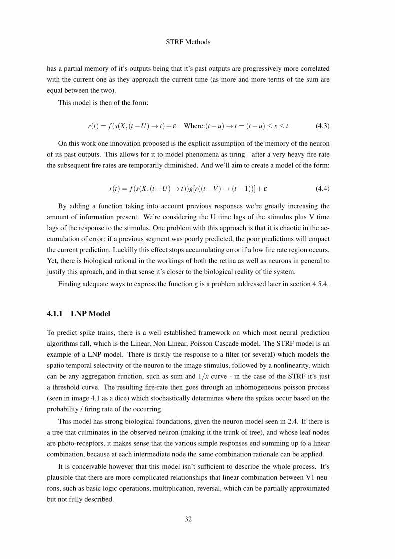
STRF Methods
has a partial memory of it’s outputs being that it’s past outputs are progressively more correlated
with the current one as they approach the current time (as more and more terms of the sum are
equal between the two).
This model is then of the form:
r(t) = f (s(X ,(t−U)→ t)+ ε Where:(t−u)→ t = (t−u)≤ x≤ t (4.3)
On this work one innovation proposed is the explicit assumption of the memory of the neuron
of its past outputs. This allows for it to model phenomena as tiring - after a very heavy fire rate
the subsequent fire rates are temporarily diminished. And we’ll aim to create a model of the form:
r(t) = f (s(X ,(t−U)→ t))g[r((t−V )→ (t−1))]+ ε (4.4)
By adding a function taking into account previous responses we’re greatly increasing the
amount of information present. We’re considering the U time lags of the stimulus plus V time
lags of the response to the stimulus. One problem with this approach is that it is chaotic in the ac-
cumulation of error: if a previous segment was poorly predicted, the poor predictions will empact
the current prediction. Luckilly this effect stops accumulating error if a low fire rate region occurs.
Yet, there is biological rational in the workings of both the retina as well as neurons in general to
justify this aproach, and in that sense it’s closer to the biological reality of the system.
Finding adequate ways to express the function g is a problem addressed later in section 4.5.4.
4.1.1 LNP Model
To predict spike trains, there is a well established framework on which most neural prediction
algorithms fall, which is the Linear, Non Linear, Poisson Cascade model. The STRF model is an
example of a LNP model. There is firstly the response to a filter (or several) which models the
spatio temporal selectivity of the neuron to the image stimulus, followed by a nonlinearity, which
can be any aggregation function, such as sum and 1/x curve - in the case of the STRF it’s just
a threshold curve. The resulting fire-rate then goes through an inhomogeneous poisson process
(seen in image 4.1 as a dice) which stochastically determines where the spikes occur based on the
probability / firing rate of the occurring.
This model has strong biological foundations, given the neuron model seen in 2.4. If there is
a tree that culminates in the observed neuron (making it the trunk of tree), and whose leaf nodes
are photo-receptors, it makes sense that the various simple responses end summing up to a linear
combination, because at each intermediate node the same combination rationale can be applied.
It is conceivable however that this model isn’t sufficient to describe the whole process. It’s
plausible that there are more complicated relationships that linear combination between V1 neu-
rons, such as basic logic operations, multiplication, reversal, which can be partially approximated
but not fully described.
32

STRF Methods
Figure 4.1: The LNP Model - The linear combination of responses of the stimulus to a filter arethen passed through a non-linearity function and then the spikes occur randomly following a Pois-son distribution whose parameters are constrained by the instantaneous firing rate. The diagramshows for simple neurons (A) of the V1 cortex there is only one prefered direction and spatialfrequency. For complex neurons often the combination of several filters is needed to approximatetheir response (B). In the bottom the STA and STC are shown to a stimulus of black and whitebars presented to the subject. The idea is to create moving windows. By averaging the resultingwindows STA is created, by estimating the covariance STC is calculated .[RSMS05]
4.2 Image Domain
The stimulus s(Xi, t) is for all practical reasons in this work, a film : a sequence of image frames
shown at periodic periods of time. Another more intuitive representation could be s(i, j, t), where
i and j are the pixel coordinates of the image, and t the frame number. The abstraction Xi is just
for generalization, and because the stimulus may not necessarily be on the form of an image and
the equations of the previous section hold true if s is something else such as sound, or the channel
values of a wavelet transform.
Ths stimulus provided in the Neural Prediction Challenge can be seen in figure 4.2.
33

STRF Methods
Figure 4.2: Typical frames from the stimulus. Top: This is the "high quality version" at 136×136resolution. These are the images shown to the subject primates in their native resolution. Clip sizevaries from 8000 to 20000 frames - up to 320s. Bottom : Low resolution down-sampled segmentof the region of interest - determined by STA
4.2.1 STA and STC
In the image domain there are two quantities that can be constructed which give information about
the response. If we take the average of all exhibited frames which trigger a neuron spike we have
gathered some information about what makes the neuron fire... the zones whose activity provokes
a greater response will be more expressed and have greater average values. Its useful to take into
consideration the STA of current spike in function of the previous stimuli. Thus usually a STA is
defined over a window of TSTA samples of length. The definition of STA is expressed in equation
4.5.
STA =T
∑i=1
yis(t→ t−TSTA)
∑yi(4.5)
Where yi is the spike count for that time frame (if the data comes in a PSTH form). If we do
it with spikes instead of PSTH, yi simply becomes 1. s(t → t−TSTA) denotes the stimuli in the
given time frames. (Can concatenated and extracted at the end, or the operation can be performed
to each value of t individually).
The process can be seen in figure 4.1 or in more detail in figure 4.3.
A problem with simple STA is that if there are constant characteristics in the stimuli (such as
34

STRF Methods
Figure 4.3: In this figure it’s possible to see in more detail the computation resulting in an STA.[Wik13c]
a white or corner) it is going to get expressed in all the frames and thus be in the final STA despite
having contributed nothing (or at least the contribution cannot be verified) to the response. If the
stimuli is white noise, or at least well distributed in terms of variance and average everywhere,
then the average over time is 0.5 (from 0 to 1 in luminosity of the pixel) and that yields great
information in the STA, because inhibition zones are also shown by being lower than average in
the STA. To try and counter this, one can "whiten" the STA, trying to make each channel average
and variance similar to white noise. To that purpose we can divide by the covariance matrix of the
stimulus:
STA = (1T
T
∑i
s(t→ t−TSTA)s(t→ t−TSTA)T )−1
T
∑i=1
yis(t→ t−TSTA)
∑yi(4.6)
Where AT denotes the transposed matrix - the first term of equation 4.6 is the Covariance Matrix.
This makes STA applicable in natural vision movies such as our data.
Spike Triggered Covariance is a related analysis tool. Having the advantage of finding a
multi-dimensional feature space for the STRF (as opposed to STA which only provides the tri-
dimensional space of the movie), the eigenvectors of STC−C (where C is the Covariance matrix
such as the one defined in equation 4.6 - not the inverse though) inform over the excitatory or
inhibitory nature by being positive or negative respectively.
The definition of STC is as follows:
STC =1
ns−1
T
∑i=1
yi(s(t→ t−TSTA)−STA)(s(t→ TSTA)T (4.7)
In figure 4.4 sample results of the application of these methods to our data yield the following.
35

STRF Methods
Figure 4.4: Top Row: STA results for TSTA = 4 for neuron 206B. RTA and RTC mean the samething as STA and STC but are used when instead of a spike train we use a PSTH to calculate- Response Triggered Average instead of Spike Triggered Average. For the various delays it’spossible to see a gabor like structure forming, with low spatial frequency - This STA can be usedto generate predictions by convolving it with the stimuli (though with very low quality). Bottomtwo rows: STC Projections : STC is a matrix whose orthogonal projection STC1 and STC2 areused as values for a latter stage of optimization and can be used for creating predictions by linearcombination.The visualization of the projections elucidates as to the direction vectors which mostaffect the response.
STA and RTC as neural response predictors have long been surpassed and provide poor re-
sults in the later stages of combination and thresholding, however they are important tools in the
determination of the parameters for other algorithms, most notably they indicate well the areas of
excitatory and inhibitory behavior as well as preferred directions.
4.3 Gabor Wavelet Transform
Representing visual information of a film on the form of images across time is very intuitive
and practical, yet information in the frequency domain is more linearly related to the observed
response [DG05]. With that in mind some algorithms emerged which first transform the stimulus
to it’s Fourier power components and only then try to apply linear combination, optimization and
further stages of processing. The current state of the art approach consists of a discrete wavelet
transform with Gabor Wavelets - by other words - the response to a filter bank. A Gabor wavelet
is a sine plane wave multiplied by a gaussian. It is well known that Gabor Wavelets model very
well the responses of simple V1 neurons [Dau80]. Another proof of the adequation of this type of
filter to video description is the fact that it’s a video compression technology used with effect in
some of today’s codecs [ERK90][LK92] for it’s capacity to describe visual structures in the way
in which we perceive them.
36

STRF Methods
A gabor wavelet or filter is of the form:
g(x,y,λ ,θ ,φ ,σ ,γ) = e−(xcosθ+ysinθ)2+γ2(−xsinθ+ycosθ)2
2σ2
× ei(2πxcosθ+ysinθ
λ+φ) (4.8)
Where λ is a the spatial wavelength, θ is the orientation, φ is the offset, σ is the standard
deviation of the gaussian, and γ is the spatial aspect ratio. An example gabor filter is shown in
figure 4.5.
Figure 4.5: 3D visualization of a Gabor Filter - This is a single specimen, a filter bank is made outof thousands like these, varying in orientation, placement, frequency amongst other parameters.This filter is multiplied together with a motion function by the video to generate a single channel,a signal varying over time.
The responses of the neurons are to ’activity’ in a given preferred orientation/zone , so we
create 3D filters consisting of a 2D Gabor Wavelet appearing and disappearing across time at a
given velocity.
For the Gabor transform of the video we use the following parameters for the wavelets (the
Gabor filters):
• Orientation
• Spatial Frequency
• Position
• Velocity
• Time Span
37

STRF Methods
• Size
• Imaginary representation
These amounts of parameters make the filter bank very large in terms of channels. It’s easy
enough to create huge banks even with small subsets of these parameters. In section 3.3 we’ve
established that orientation selectivity is around 3o to 10o, and only 180o should be covered (the
response is simply negative if the direction is opposite), therefor we can estimate the filter bank to
require between 18 and 60 divisions.
One good solution to obtain large representation of frequencies, is to use logarithmically
spaced frequencies from covering the entire image to a sharp line.
We establish a grid of position of application of the filter, rendering the offset obsolete (it’s
essentially the same thing but with more freedom, as we can also translate transverse, instead of
just in the direction of the orientation). The size of the filter bank reached 40000 in some tests
(which is rather large comparing with the 16× 16 image at hand), but good values were found
at size 6000. Too large filter banks increase the dimensionality of the optimization and have
downsides, though some algorithms handle it better than others. In figure 4.6 an example of a used
gabor filter is shown.
Figure 4.6: A single gabor 3D filter, with a temporal size of 9. From left to right temporal indexes: -4 to 4. The Gabor filters have a sensitivity to changing features. This particular one has ashort temporal velocity and a low spatial frequency. This is a channel representing the half waverectified real part |Re(g)|+
4.4 Optimization Algorithms
The middle part of the LNP model requires iterative processes of optimization - these vary in
terms of speed, final result, resistance to noise, resistance to undersampled values, handling of
high-dimensionality, and can make all the difference in terms of the final quality of the achieved
solution. sub
4.4.1 Gradient Descent
Finding the best way to combine linearly all the stimulus channels (in whatever form they may be,
such as image pixels, responses to STA and STC or wavelet channels) is a problem of optimization.
The Gradient Descent concept simply describes a method of finding local minima from a starting
point by going down the gradient. Very much alike being at the top of a mountain blinded - if
38

STRF Methods
one wishes to get to the lower ground, or more precisely reach the bottom of the valley below, a
simple method is at each step to determine the orientation of the slope of the ground, and give the
next step in that direction - it’s so intuitive most of us would proceed that way without thinking
about it. It may not guarantee the shortest path (the shortest path may be over a lower mountain in
the way, and we would go around by using this method) but it’s the simple base to the problem of
regression at hand.
The minima we’re trying to find is the error of the solution, and the slope can be estimated by
the current position.
Let Wi be the array of weights for all N channels of the feature space Si i = 1→N, such that:
rp(t) =N
∑i=1
WiSi (4.9)
Where rp(t) is the predicted response for time t.
Then we can define the error of that prediction as the difference between the predicted value
and the real observed response:
ε(t) = rp(t)− r(t) (4.10)
Let’s start by initializing the Weight Vector to 0. For each sample in the response we can add
to the Weight vector the features which triggered that response:
W 0i = 0 ,0 < i≤ N (4.11)
For the general case Gradient Descent, the approximation is as follows:
W k+1 =W k + γ∇ε(W k) (4.12)
Where γ is the step size, ∇ the gradient operator and ε(Xk) denotes the error function in respect
to the weight vector W ( as opposed to ε(t) which is the error of a given time frame).
Applying equation 4.12 to a single channel / weight, and using the estimation of gradient
∇ε(Xi) = ε.S we arrive at the following expression for tor an individual feature:
W k+1i =
Nsamples
∑t=0
W ki +Si(t).ε(t) ,0 < k ≤ N (4.13)
W ki denotes the Weight of the i’th channel after iteration k. Equation 4.13 can be read as :
in each iteration add to the weight the average of the error of the current solution multiplied by
the stimulus which produced that error. That means that after each iteration each weight will get
adjusted by the average of how that weight affected the prediction.
In our particular case we have a stimulus and several time delays which may affect the re-
sponse, mathematically it’s the exact same thing, it can be worked by extending the feature domain
over the chose time frames of delay, but for clarity consider the following method of computation
as implemented in this work.
39
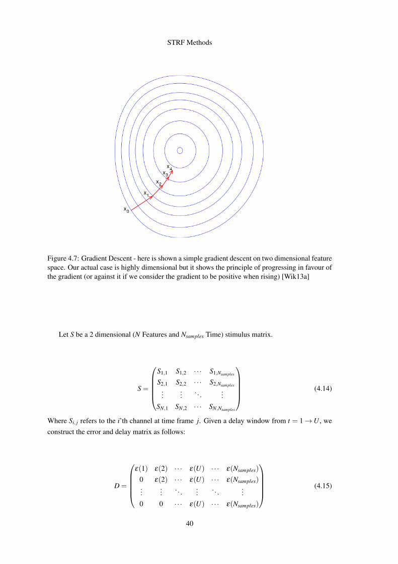
STRF Methods
Figure 4.7: Gradient Descent - here is shown a simple gradient descent on two dimensional featurespace. Our actual case is highly dimensional but it shows the principle of progressing in favour ofthe gradient (or against it if we consider the gradient to be positive when rising) [Wik13a]
Let S be a 2 dimensional (N Features and Nsamples Time) stimulus matrix.
S =
S1,1 S1,2 · · · S1,Nsamples
S2,1 S2,2 · · · S2,Nsamples
......
. . ....
SN,1 SN,2 · · · SN,Nsamples
(4.14)
Where Si, j refers to the i’th channel at time frame j. Given a delay window from t = 1→U , we
construct the error and delay matrix as follows:
D =
ε(1) ε(2) · · · ε(U) · · · ε(Nsamples)
0 ε(2) · · · ε(U) · · · ε(Nsamples)...
.... . .
.... . .
...
0 0 · · · ε(U) · · · ε(Nsamples)
(4.15)
40

STRF Methods
By multiplying D× ST we have for every sample in row j the proposed gradient estimation
based on that sample:
∇ε = D×ST =
∑
Nsamplec=1 S1,cε(1) ∑
Nsamplec=1 S2,cε(2) · · · ∑
Nsamplec=1 SN,cε(N)
∑Nsamplec=2 S1,cε(1) ∑
Nsamplec=2 S2,cε(2) · · · ∑
Nsamplec=2 SN,cε(N)
......
. . ....
∑Nsamplec=U S1,cε(1) ∑
Nsamplec=U S2,cε(2) · · · ∑
Nsamplec=U SN,cε(N))
(4.16)
In matrix D× ST we have the estimation of the gradient by multiplication of every sample’s
error with the features of that sample at a given time delay. Alternatively we could have condensed
the time delays in a single line and handled the entire thing as a greater extent feature space, but this
description is faithful to the MATLAB implemented version - which takes greater computational
advantage of this form as it allows MATLAB’s highly optimized matrix computation to be used
and is significantly faster than iteratively calculating all values involved with for loops.
4.4.1.1 Momentum
Momentum in the gradient descent is the concept of using the past gradient combined with the
current one.
∇mεk+1 = ∇ε
k+1 + v∇mεk (4.17)
The inclusion of momentum is convenient cases where the hyper-surface of the error function
contains some noise. By including moment the algorithm passes over small pieces of noise that
would otherwise cause a slowdown. On the approach with the minima momentum also helps
correcting the zig zag of going back and forth around the depression (as they average a little).
A typical value for the momentum would be v = 0.5. By comparison with simple feedback LTI
closed ring systems we can clearly see that this is a simple low pass filter upon the gradient.
4.4.1.2 Norm of the Gradient
The step size used for each new iteration is an important parameters of the optimization algorithm.
A small step size assures precision in getting near the true minimum, but is very slow to arrive
there. A large step size will quickly arrive at a solution approximate from the minimum but
will not approach it completely going back and forth over the minimum in a zig zag pattern. One
possible solution to this problem is to divide by the error, this ensures that the step size is governed
by the defined parameter and will minimize overshoo. One problem with this aproach is that the
minimum error is not zero, only if everything were ideal would this mechanism be feasible. In
fact at the start of the algorithm we know that the minimum is less than or equal to the initial
estimation but it can be any value between 0 and that value. Another candidate for an estimation
of "how close" we are to the minimum is the magnitude or Norm of the gradient. If we divide the
41

STRF Methods
step by the gradient’s norm we’ll get step sizes which are large enough when the gradient is very
low, and small enough when the gradient is very high, rendering the algorithm resilient to high
spatial frequencies.
The expression for the update of the coefficients becomes:
W k+1 =W k +γ∇ε(W k)
||∇ε(W k)||(4.18)
Where ||X || denotes the euclidean norm of vector X .
4.4.2 Coordinated Gradient Descent
In very high dimensional cases of "exploratory" linear combination (exploratory in the sense we
only use a high number of features because we don’t know which might actually be used, rather
than we expect them all to contribute somehow) it may be useful only to add the greatest compo-
nent of the gradient. This is called Coordinated Gradient Descent because effectively we’re only
going along a coordinate at at time. The gradient is thus reduced to it’s maximum component as
seen in equation 4.19.
∇εCoordinated = max(∇ε) (4.19)
One limitation of CGD in high dimensional data is that it has some trouble getting the impor-
tant coefficients adjusted right. It will detect them and get them near their perfect value early on,
but then because they are close it is not likely to touch them again, favoring noisy alternatives best,
and in high dimensional data is easy to find uncorrelated features louder than the required adjust
at the important ones.
4.4.3 LARS
The Least Angle Regression method is a good tool from high-dimensional statistics. It’ has "fea-
ture selection" like operation, and is computationally as efficient as the forward selection algo-
rithm. It is stable and well correlated features with the response will get their coefficients updated
at roughly the same rate.
The algorithm relies on the correlation between each feature vector and the output, adding
the best. And as soon as the information achieved by others makes them redundant, removing
them.[EHJT04]
The algorithm is as follows:
1. Start with all coefficients Wi equal to zero.
2. Find the predictor Sa most correlated with r(t) by taking the correlation of all features vs
response
3. Increase the coefficient Wa in the direction of the sign of its correlation with r(t). Take
residuals ε = r(t)− rp(t);
42

STRF Methods
4. Stop when some other predictor Sb has as much correlation as Wa.
5. Increase (Wa,Wb) in their joint least squares direction, until some other predictor Sc has as
much correlation with the residual ε .
6. If any SiWi is now less predictive than a member outside the ensemble, drop it.
7. Continue until: all predictors are in the model, the stopping set has started diverging, or
maximum iterations reached.
4.4.4 Thresholded Gradient Descent
This is the state of the art method in terms of results [NPC]. It’s a simple gradient descent (imple-
menting momentum, adaptative steps) where we define two thresholds : θ and θG , respectively
the channel threshold and the group threshold.
We start with an empty set of active channels. In the gradient estimation matrix as obtained by
equation 4.16 we add values above θ ×max(∇) to the active set. Furthermore for each time frame
(each line in the matrix) we remove those that are below θG of the maximum of the group. This
allows for the selection of the most relevant features, and to prune those in each time frame which
have sub-average performance (they can be above the global threshold because the frame which
generated them was very active and so most components got dilated - it’s a common phenomena
at image change moments with high motion, most components trigger highly above average for
those frames, and less important ones are "dragged" up).
This allows for the formation of a good basis of features early on with high correlation with
the response and makes the early high values of the error function not propagate so much to the
noise / poorly correlated features.[GL05]
In our case’s notation this simply translates into:
∇ε i, j = 0 if {i, j} /∈ As (4.20)
and:
{i, j} ∈ As if ∇ε i, j ≥ θmax(∇ε) ∧ ∇ε i, j ≥ θGmax(∇ε i) (4.21)
4.5 Other Methods
This section details non-optimization related techniques used.
4.5.1 KNNC
An different aproach to the steepest gradient was also used: classifiers. If we consider the various
time points as samples with an associated feature array, we can train a classifier with it. One natural
choice given the high number of samples is the KNN Classifier. KNN’s principle of operation
is tremendously simple : a new sample is classified by the majority of the k closest samples.A
43

STRF Methods
more visual explanation can be seen in figure 4.8. The advantages of this classifier over linear
combinators is that it can incorporate complete non-linear effects, being dependent only of the
quality of the data and the distribution of samples to fall on the zone of interest.
The pixels themselves of the untreated stimulus can be used as features for this classifier,
and it still yields interesting enough results. However our problem requires not a single 2 class
classification, but a multi class one. Fire counts at each bin of the PSTH can reach 11, so we have
a 12 class classification problem. This doesn’t suit KNNC very well, because classes need to be
well represented, and equally represented in interclass boundaries for the method to be reliable.
That is not the case because high spike counts are much rarer than single spikes or no spikes at
all. However, if we consider only whether the neuron fires anything or not at all, then knnc is a
formidable classifier, and can yield important information in particular about the moments when
the neuron is not expected to fire, and be combined with other methods.
Figure 4.8: KNN classification - For a new sample the class of the k closest neighbours of that sam-ple determines the classification, majority rules. From http://www.statistics4u.com/fundstat_eng/cc_classif_knn.html
4.5.2 Adaptative Threshold Fitting
This very simple technique is a way of estimating the apropriate threshold at which to clip the
response to zero. The threshold is simply varied from 0 to the max of the predicted response,
and we assess the correlation for each clipping, and chose the threshold which fits best. Often
best correlations are obtained without threshold ( 0) but it contributes to improving the response
sometimes.
44

STRF Methods
4.5.3 Resampling
It’s important when performing the classification / optimization to use both a early stopping set
:this is a subset of the sample whose data is not used in the gradient, but whose error is measured
and determines when we’re over-fitting. Two methods of re sampling were used: jackknifing
and bootstrapping. They are very similar:in jacknifing we remove a segment from the image and
optimize without it (using it as early stopping is fine, and actually convenient). In bootstrapping
we do the same thing but randomly, by creating a substitution segment and randomly substituting
parts of the training signal with subsets of the substitution segment. In both cases we used 5
iterations - 5 fold jacknifing and 5 fold bootstrapping.
The resulting filters can be averaged to yield a strf with very little biasing and over-fitting
indeed, and generally improves results upon a completely independent testing segment left out
and not used in anything from the beginning of the processing.
Two methods of re-sampling were used: jackknifing and bootstrapping. They are very similar:
in jacknifing we remove a segment from the image and optimize without it (using it as early
stopping is fine, and actually convenient). In bootstrapping we do the same thing but randomly, by
creating a substitution segment and randomly substituting parts of the training signal with subsets
of the substitution segment. In both cases we used 5 iterations - 5 fold jacknifing and 5 fold
bootstrapping.
4.5.4 NARX Networks
Nonlinear Auto Regressive Exogenous networks are a type of model, which aims to predict a
time series, based on itself, and a different time series [Dia08]. The mathematical model is of the
following form:
y(t) = F(y(t− i),y(t−2),y(t−3), · · · ,y(t−T1),x(t),x(t−1),x(t−2), · · · ,x(t−T2))+ ε (4.22)
If we look closely this is an analogous form of the model proposed in equation 4.4 (by dif-
ferent notation - this one is the canonical when describing NARX and is only applied to 1D),
which means this method fits perfectly into the idea of assigning output memory to the prediction
function, and thus modeling the response’s auto correlation. The applications of this model excel
in time-series prediction (the response is a time series) from another time series (the predicted
response). Thus we can have in our notation:
rp(t) = F(rp(t− i),rp(t−2),rp(t−3), · · · ,rp(t−U),r(t),r(t−1),r(t−2), · · · ,r(t−V ))+ ε
(4.23)
Where U and V are the maximum delays to be considered in the feedback and exogenous signal
respectively. This equation can be used for trainning the function F, which is a Neural Network
with the layout shown in figure 4.9. The topology in question is called open loop, because we allow
45

STRF Methods
for the feedback and exogenous signal to be fed directly to the classifier, because we possess both.
This is necessary to simplify training, because as we insert a true feedback circuit the complexity
is going to increase exponentially in the backpropagation learning algorithm [mata].
Figure 4.9: Matlab’s nntrain tool, showing the network model begin trained - open loop, in theclosed loop the output y(t) is connected to the incoming y(t)
One thing of mention regarding the use of NARX, is that it may be somewhat stochastic. The
values used for the initialization of the neuron weights and bias are randomly generated. We’ve
used a constant seed to maintain results consistent, but when using the tools, the small changes of
performance from trial to trial are to be expected, if the reader atempts a parallell implementation.
4.6 Computational Implementation
The chosen language and environment for this work was Matlab R©v2013a. For the tests with
neural networks and classifiers of which knn emerged as the best, prtools - Pattern Recognition
Tools library v 4.2.4 28 was used. It consists of a good abstraction layer for handling machine
learning, through a powerful "dataset" general class to describe data, and apropriate tools for
training, visualization, validation and deploying created solutions.
The strflab library v1.45 was used, it implements most of the concepts, it borrows heavily
from netc statistical models library, and implements most of the functions described in this work.
Certain enhancements were made. strflab also contains the 2nd best method-state of the art, which
is from a colleague of the library’s developer. The current state of the art code was supplied on
request by the involved researcher which is also the creator and maintainer of strflab.
In previous works by the author, Matlab Distributed Computation Server was used to take full
advantage of the author’s computers computational resources (see table 4.1). Sadly the evaluation
license expired mid-way so there was need to devise a "poor-man’s" work distribution center. For
46

STRF Methods
Table 4.1: Computational Resources Available for Processing
Machine 1 - Panther ServerProcessor Intel Core 3570k @ 4.2GhzMemory 32 GB DDR3 1600MHzGPGPU Nvidia GTX 660 Ti @ 1100 MHz 2.6 TFLOPS
Machine 2 - Königstiger ClientProcessor Intel Core 3930k @ 4.5GHzMemory 32 GB DDR3 1600MHzGPGPU ATI 6970 @ 950 MHz 2.7 TFLOPS
Machine 3 - PzKw III ClientProcessor AMD Phenom II 955 @ 4GHzMemory 4 GB DDR2 1333MHzGPGPU None - Graphics card doesn’t support
this case the full data files, scripts, functions and libraries were placed on each of the computers
and a small client-server architecture was devised.
4.6.1 Distributed Computing
The main focus of the distributed computing was to increase the speed of parameter sweeping, by
far the most time consuming activity of computation in this work. In this light the clients simply
connect to the server and listen for coordinates - a given trial’s parameters. The architecture is
first come first served, with a client connecting to the server, getting the next coordinates ( a set
of parameters to test) and then returns the results. It does so endlessly until the server tells it to
end the program. The server stores the results relayed by the computing nodes. This aproach is
certainly not as noble and perfect as matlab’s implementation of simulated annealing on distributed
computing platform, but it’s good enough to speed up somewhat the parameter sweeps. The server
itself is running two instances of matlab, allowing it to compute as well, at the same time as it
gathers data - however there seems to be some bugs associated with this aproach as there were
some random crashes which caused some annoyance.
4.6.2 GPU Optimization
The strflab library is very well done, with imense flexibility and excellent coding practices, and
the author is to be commended on it’s quality, it does not however implement any type of compu-
tational acceleration by GPGPU - General Purpose Graphics Processing Unit. Modern graphics
cards (and some dedicated computing cards) asides from rendering graphics, have established
themselves as titans of computation - a high-level graphics card has nowadays about 400× the
computation resources of a top class CPU. Graphics cards achieve this high performance in terms
of FLOPS (floating point operations per second) by using programmable SIMD (single instruction
multiple data) arrays which use low intelligence processing units, not unlike CPU cores, but much
47

STRF Methods
more limited in terms of instruction set and advanced conditionals like branch prediction. A dia-
gram of the two can be seen in figure 4.10. For simple operations the sheer number of cores at a
much slower speed and much lower IPC (instructions per clock cycle) can make them incredibly
more potent than a typical 4GHz Quad Core CPU.
To leverage this computing power the designed applications must be highly parallel, such is
our case. Although the algorithms used for optimization are iterative, the great computational
effort at each iteration is the convolution and multiplication of matrices, which are extremely par-
allel (one can divide the work load of matrix multiplication or convolution by different workers).
Matrix multiplication can be parallelized into single multiply and add (MAD) operations over two
perpendicular vectors for each element of the resulting matrix, and that task can be done by a
different processing core of the graphics card. Likewise convolution can be divided in time frames
with each core handling the convolution of a smaller segment of time.
In terms of convolution a speedup ceiling of 205× is possible in our system, and in terms
of matrix multiplication up to 110× of improvement was achieved in ideal settings. The real
speedups of the process are not that great however, still significant but within order of magnitude
of the original performance. One particular problem is the movement of data in and out of the
GPU (graphics processing unit) to the RAM of the computer, which despite being very fast in
terms of bitrate and transmission speeds, has a slow initiation and synchronization delay. The
implementation of the heavy workload functions of matricial computation was done trying to
minimize as much as possible these fluxes of data, but this, in conjunction with the fact that
most of the algorithms still rely on CPU and in particular matlab’s JIT based aproach instead of
native code, turn the improvements of said algorithms into 5× the original version. In very long
computations with a small step, long signals, a high number of channels and the use of resampling,
the overall efficiency speedup is near the 5× achieved in the algorithm, yet for lesser intensive
trials the other stages of the process dominate the spent time.
The two most critical functions of computation were optimized in this work, being the func-
tions that calculate the gradient and which evaluate the STRF with data error towards the response
- respectively linGrad and strErr - this was done by modifying these functions to use GPU opti-
mized subroutines also adapted in this work which perform the calculations -linGradTimeDomain
and linFwd.
To assess and improve the performance of the various stages of the algorithm Matlab’s profiler
tool was used. This tool discriminates exactly how much time was spent in each line of code, and
at which functions and child functions all the way down to Matlab’s core essentials.
Seen in annexes, are the differences between the same exact test run on GPU optimized calcu-
lation of the gradient and standard CPU one.
Another, and perhaps more fortuitous performance improvement was discovered in a 2272s
trial: it was discovered using the profiler that the Threshold Gradient Descent - not included in
strflab, still unpublished work by the library’s author and state of the art current holder, which
he made available for the purpose of this work - spent exactly 2000.65s in a poorly placed "find"
operation which when substituted by a more convenient direct index mapping reduced to 200s the
48

STRF Methods
Figure 4.10: Illustration of the differences between a CPU and a GPU. The higher core countmakes processing on the GPU much faster. The data transmission between both must however bekept to a minimum, as it can slow the process significantly.[matb]
execution of this block of code. In this particular intensive trial the speed up was from roughly
one hour to about ten minutes on the same machine, and thus immediately raises the contribution
of this work to the state of the art as a 6× improvement in speed.
Given that the author of the strflab library has not given express permition to print his work,
the code listings of strflab changed functions are presented in minimal scope. In annex the perfor-
mance enhancement is shown from a printscreen of profiler.
49

STRF Methods
50

Chapter 5
Results
In this chapter the results from the conducted trials are presented. The pValues represent the
probability of the given result being a random event between two uncorrelated distributions, and
are a measurment of the statistical reliability of the result. The pValue is obtained by the pairwise
comparison of the measurements using matlab’s corr.
5.1 Measurement of Performance
The chosen criteria by the Neural Prediction Challenge is the correlation between the predicted
neural response and the observed one. In particular Pearson’s product-moment correlation coeffi-
cient (also known simply as Pearson’s R). It was formulated by Karl Pearson, as the covariance of
the two variables over the product of their standard deviations.
r =cov(X ,Y )
σX σY=
E[(X−µx)(Y −µy)]
σX σY(5.1)
Which on a sample by sample base can be derived by the estimators:
r =
n
∑i=1
(Xi− X)(Yi− Y )√n
∑i=1
(Xi− X)
√n
∑i=1
(Yi− Y )
(5.2)
This measure of performance can be criticized, firstly because it’s insensitive to the mean
of the variables, and because it assumes a normal distribution. The first is completely counter
purposeful in the given situation, it’s important not only to predict when the spikes occur but as
well the magnitude (in terms of number of spikes per time bin). Ignoring the average ranks equally
two predictions, with the same shape, but translated. The second, is well known not to be the case,
the firing of neurons in a given time frame behaves in a Poisson Process manner [KV01], and thus
has a Poisson Distribution of probability density function.
51

Results
Regardless the authors of the challenge claim, that being that this measure is the most often
employed one in the literature and previous tests (and everyone is probably already familiar with
it) it is the one to be used.
5.2 Parameter Sweep
The overall free parameters and variations of methods make such a great extent of combinations
that parameter sweeps, although extremely thorough in the opinion of the author, and taking ad-
vantage of the various speedups and relatively sophisticated domestic computational resources of
the author, could not plausibly browse through.
5.2.1 Available Methods
5.2.1.1 Resolution
Starting with methods combinations, one has the opportunity of using the low quality 16× 16
resolution, the full resolution stimuli (136× 136) or a cropped center of an arbitrary dimension
(it was used by other works with agreeable results at dimension 32×32). The size of the stimuli
doesn’t affect the greates extent of the computation time which is in optimization. Once the Gabor
Wavelet is done, the number of channels is the same, yet to obtain the same spatial frequency detail
if one used an image which covers a greater part of the image , the density of application of Gabor
Filters must be increased, therefor a greater resolution will force the use of more channels for the
same detail. With the low performance algorithm STA/STC because the pixels themselves can
be used, resolution does affect proportionally computation time, and the high resolution stimuli
becomes a heavy computation, yet there appear to be no improvements in results.
Regardless the variations defined for the parameter of resolution are:
1. Downsampled 16×16 stimulus
2. Cropped 32×32 center of high resolution stimulus
3. Full 136×136 stimulus
5.2.1.2 Optimization Method
The Optimization Methods are described in the Methods section, they are by crescent order of
performance:
1. Simple Gradient Descent - With Momentum and Norm factoring and adaptive step
2. Coordinate Descent
3. LARS
4. Threshold Gradient Descent
52

Results
Other methods including direct fit (similar to an averaged KNN) and Neural Networks were
attempted but without promising results that warrant being pursued any further. The idea behind
SGD and CGD are that if the result could be improved by getting better features they might com-
bine them well enough - if the lacking part of the solution was detail, or amount of channels, they
would be able to leverage the information into better results.
5.2.1.3 Train Percentage
The amount of data used for validation and training actually seems to influence the results more
than anticipated. It was to be expected that the higher the percentage of data used for trainning
the better the result, but with less statistical validity. However, as we increase the percentage of
training above 70%, the validation correlation rate starts decreasing. The proposed explanation is
that by reducing the validation set, we’re increasing the impact of noise. As we average over more
frames the actual qualities of the method statistically compensate.
The sweep contraints are step = 0.5→ 0.9 at ∆step = 0.1.
5.2.1.4 Delays to use
The information taken from STA/STC shows that most of the response is governed by the first
nine frames of the response, thus we propose that the delays screening as follows.
U = 7→ 15 with ∆U = 2
Though several experiments we delays of 20 and 30 were used. 30 being the number of time
frames between image change (0.5s) of the stimulus. Nine was indeed found to be the perfect
value for all but 3 of the neurons in which it was 7.
5.2.2 NARXdelays
The delays of the response to consider in the NARX network. Too much and it becomes noisy and
hampers learning, too little and there is no sufficient information for a basis of decision. The other
delay (U in our nomenclature regarding NARX) is set to 2, the algorithm only considers current
prevision and past prevision, that way, information on the derivative is present to the classifier,
allowing it to know not only the predicted fire rate , but how it’s varying. This allows to model
things like pre-emptive fire. If the response is rising rapidly the network tens to increase the peaks
quicker, allowing for a good piece of non-linearity closely related to biological behavior.
5.2.3 Thresholds
Both the global and the group threshold used in the Threshold Gradient Descent are very data
dependent.
The search window used was: θ ,θG = 0→ 1 with ∆θ ,∆θG = 0.1
53
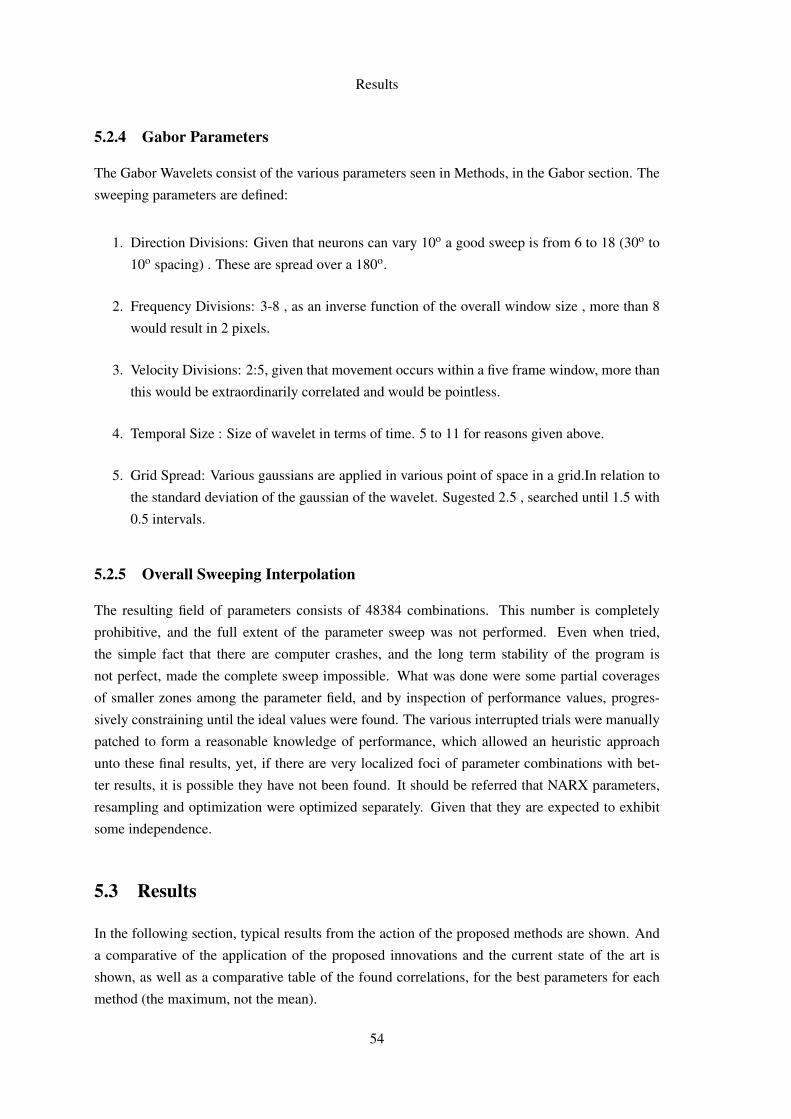
Results
5.2.4 Gabor Parameters
The Gabor Wavelets consist of the various parameters seen in Methods, in the Gabor section. The
sweeping parameters are defined:
1. Direction Divisions: Given that neurons can vary 10o a good sweep is from 6 to 18 (30o to
10o spacing) . These are spread over a 180o.
2. Frequency Divisions: 3-8 , as an inverse function of the overall window size , more than 8
would result in 2 pixels.
3. Velocity Divisions: 2:5, given that movement occurs within a five frame window, more than
this would be extraordinarily correlated and would be pointless.
4. Temporal Size : Size of wavelet in terms of time. 5 to 11 for reasons given above.
5. Grid Spread: Various gaussians are applied in various point of space in a grid.In relation to
the standard deviation of the gaussian of the wavelet. Sugested 2.5 , searched until 1.5 with
0.5 intervals.
5.2.5 Overall Sweeping Interpolation
The resulting field of parameters consists of 48384 combinations. This number is completely
prohibitive, and the full extent of the parameter sweep was not performed. Even when tried,
the simple fact that there are computer crashes, and the long term stability of the program is
not perfect, made the complete sweep impossible. What was done were some partial coverages
of smaller zones among the parameter field, and by inspection of performance values, progres-
sively constraining until the ideal values were found. The various interrupted trials were manually
patched to form a reasonable knowledge of performance, which allowed an heuristic approach
unto these final results, yet, if there are very localized foci of parameter combinations with bet-
ter results, it is possible they have not been found. It should be referred that NARX parameters,
resampling and optimization were optimized separately. Given that they are expected to exhibit
some independence.
5.3 Results
In the following section, typical results from the action of the proposed methods are shown. And
a comparative of the application of the proposed innovations and the current state of the art is
shown, as well as a comparative table of the found correlations, for the best parameters for each
method (the maximum, not the mean).
54

Results
5.3.1 Wavelet Transform
The diversity of parameters can make a graph of the evolution of them all difficult to comprehend,
essentially in each line is a channel, and these channels are the convolution of a filter of Gabor
kernels which describe the image (becoming a form of wavelet transform) - seen in figure 5.1 is
a clipped subspace of the stimulus after being decomposed into wavelet channels. It’s easy to see
the problem of dimensionality and computation cost when we consider that we obtain that from a
16×16 stimulus across 15s in time.
Figure 5.1: 3D graph of 1000 channels over 15s time period (900 samples), notice the periodicspikes across most channels. When there is motion in the image most channels rise, this makesthe channels extremely correlated amongst themselves, and causes to consider if some dimen-sionality reduction by joining similar channels wouldn’t be positive for something else apart fromperformance.
5.3.2 Adaptive Threshold
The curve of performance for a threshold array is always computed, and the maximum is chosen
as the final response. Typical curve shown in fig. 5.2.
5.3.3 Legacy STA / STC
With correlation values in the 0 to 0.25 range, STA STC shows it’s obsoleteness. KNN does a
better job for a image domain algorithm in terms of results. Yet this algorithm was an absolute
must for it’s the historical way (since the 50’s) that the visual cortex has been analyzed. An
example of training can be seen in figure 5.3.
Yet there are some merits to it, in terms of allowing the visualization of the field of view
responsible for the activation of the neuron STA/STC still gives practical results as seen in figure
5.4.
55

Results
Figure 5.2
56
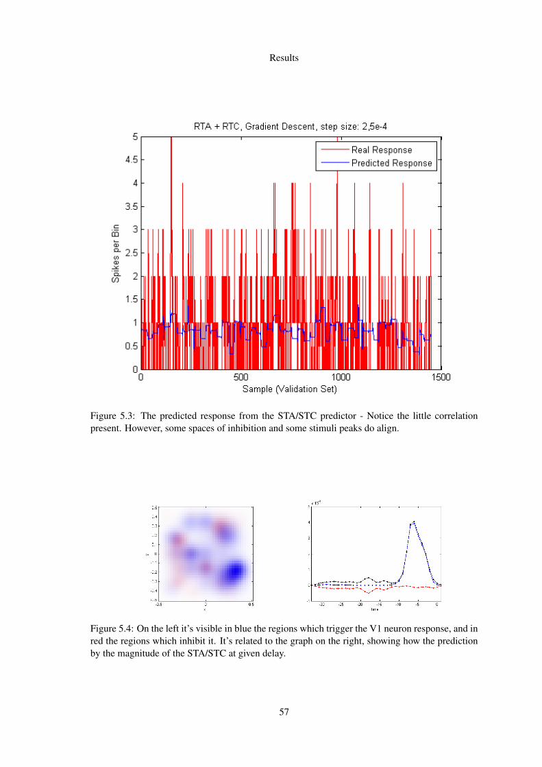
Results
Figure 5.3: The predicted response from the STA/STC predictor - Notice the little correlationpresent. However, some spaces of inhibition and some stimuli peaks do align.
Figure 5.4: On the left it’s visible in blue the regions which trigger the V1 neuron response, and inred the regions which inhibit it. It’s related to the graph on the right, showing how the predictionby the magnitude of the STA/STC at given delay.
57

Results
5.3.4 Gradient Descent
Gradient Descent results were somewhat disapointing. Expectations weren’t high to begin with,
but with large numbers of feaures it was somewhat expected that it’s simplicity and greater speed
would actually turn up some decent results.
Figure 5.5: Typical training graph of a Simple Gradient Descent - on the left, the resulting weights- on the center: the training set error, on the right: the early stop set error - As soon as the errorstarts to increase in the early stop set, it means that the algorithm is overfitting in the training set,and the solution is no longer improving for an unbiased sample.
It does converge pretty fast, and is an excellent pivot point to anchor comparisons between
parameters.
5.3.5 Coordinated Gradient Descent
As expected CGD converges slowly but steadily onto solutions more perfect than simple GD. This
comes for it’s method of only editing one weight a time. Given the high dimensionality of the
problem, with thousands of channels it’s no surprise this algorithm takes thousands of iterations
to reach completion. Typical convergence of CGD is shown in figure 5.6.
5.3.6 LARS
LARS path towards the solution looks a little more ragged than most, yet it’s remarkable how
it converges in so little iterations. This is the result of using the best correlation rather than the
gradient descent estimation as source of information on which parameters to update. This comes
at the cost that each LARS iteration is much more heavy than the corresponding gradient descent
approaches, and takes much more time. The process is seen in figure 5.7.
58

Results
Figure 5.6: It can be seen the difference of emphasis given in the Coordinate Descent, by therelative scarcity of the Weights, and it’s also visible that this optimization takes a lot of iterationsto reach it’s minimum.
Figure 5.7: The correlation aproach makes the LARS algorithm show a weight array not unlikethe Coordinate Descent, with few weights but meaningful. It converges rapidly
59
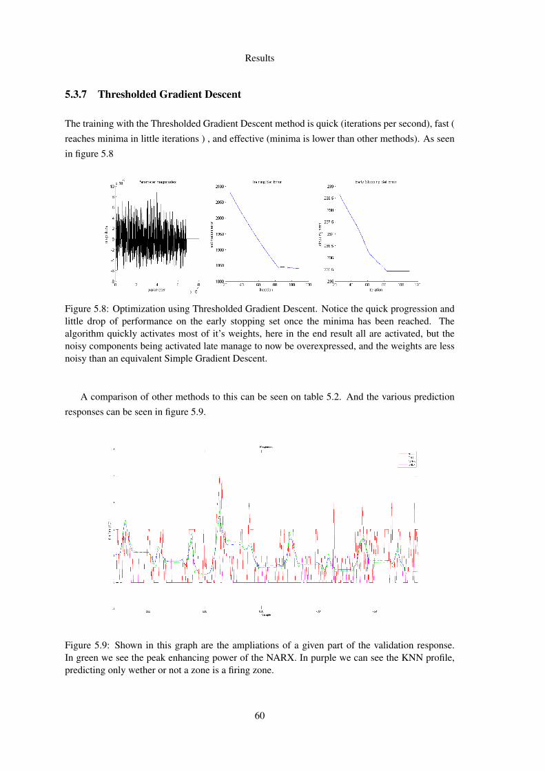
Results
5.3.7 Thresholded Gradient Descent
The training with the Thresholded Gradient Descent method is quick (iterations per second), fast (
reaches minima in little iterations ) , and effective (minima is lower than other methods). As seen
in figure 5.8
Figure 5.8: Optimization using Thresholded Gradient Descent. Notice the quick progression andlittle drop of performance on the early stopping set once the minima has been reached. Thealgorithm quickly activates most of it’s weights, here in the end result all are activated, but thenoisy components being activated late manage to now be overexpressed, and the weights are lessnoisy than an equivalent Simple Gradient Descent.
A comparison of other methods to this can be seen on table 5.2. And the various prediction
responses can be seen in figure 5.9.
Figure 5.9: Shown in this graph are the ampliations of a given part of the validation response.In green we see the peak enhancing power of the NARX. In purple we can see the KNN profile,predicting only wether or not a zone is a firing zone.
60

Results
sTable 5.1: KNN’s response confusion matrix
True Labels Estimated Labels
0 1 Totals0 603 329 9321 344 512 858Totals 947 843 1790
5.3.8 KNN
The performance values of KNN are not great, averaging 0.35 correlation, however the correlation
is exceptionally high because for the given testing algorithm it’s as bad to miss from 0 to 1 as from
1 to 7. Yet we know that it carries predicting power distinguishing fire zones with effectiveness as
seen in table 5.1.The discriminating power can also be seen in figure 5.10.
Figure 5.10: Shown in this graph are the original response in blue, vs the predicted by the KNNcclassifer in red. This high quality temporal information can be of great use in future models.
61

Results
Table 5.2: Comparison of Relative Performance among methods
Method Relative Performance
STA/STC 34%1
SGD 74%CGD 79%LARS 89 %TGD 100%
5.4 Final Results
The results using the best parameters, and including the contribution, Threshold Fitting, NARX
processing, Thresholded Gradient Descent. The best parameters are the best overall parameters,
there was no adaptation for each individual neuron - for the idea is to establish a solid func-
tional algorithm, not waste the user’s time performing very large time consuming parameters
sweeps.[ZD13]
Parameters for maximization : θG = 0.6 θ = 0.8 DirDiv = 16 VDiv = 3 FDiv = 4 K =
7 γ = 3E−4 Res = 16×16 U = 9 V = 9
The results can be seen in table 5.3. The very low p Values should be perceived in the light that
there are many samples ( 15000 mean). The results for neuron “r0220A” were excluded from the
computation of the mean improvement result. It’s not only the doubful p-value, which could have
been artificially increased by using cross validation, it’s the fact that by inspection there looks to
be only incidental fitting in both algorithms. There was no actual improvement, and the superior
values are but random coincidence, as all algorithms ever tried in the neural prediction challenge
fail to predict at all (like ours) with any discriminant power for this neuron. Therefor, the author
feels it’s more honest to exclude the extra 1% improvement this part of the dataset would provide.
62

Results
Table 5.3: Final Results from the best solution found
Performance Comparative
Neuron Correlation value State of the Art Correlation Improvement p Value
r0206B 0.6694 0.6631 1% 0.000r0208D 0.4032 0.4062 -1% 0.001r0210A 0.5049 0.4902 3% 0.003r0211A 0.4728 0.4669 1% 0.001r0212B 0.4642 0.4576 1% 0.003r0217B 0.4091 0.4102 -3% 0.001r0219B 0.5249 0.5050 4% 0.001r0220A 0.1654 0.1428 16% 0.1204r0221A 0.6164 0.6037 3% 0.000r0222A 0.4563 0.4694 0% 0.002r0223A 0.4918 0.4411 3% 0.001r0225C 0.4156 0.4127 1% 0.001Average 0.4662 0.4557 2%*
*-Doesn’t include r0220A as it’s clearly ineffective there
63

Results
64

Chapter 6
Conclusions and Future Work
The outcome of this work is definitively a most positive one. The results explicit a small but
consistent improvement over previous methods. This improvement is only natural as it relies on
what may be derogatorily called "post-processing tricks" and the already state of the art method,
yet, given the evolution that the field of neural prediction has taken over the last few years, these
tricks seem appropriate. Another thing that makes the novel methods suggested on this work more
worthy, is that the field of regression, optimization and statistical analyzes in high dimensionality
is very well established with a great many types of algorithms and statistics dominating the field.
Innovating on the fundamentals of neural prediction thus becomes hard. The major innovation in
the author’s perspective in this is the usage of NARX networks, because they appeal to the idea
that the current model which does not include previous response memory is wrong. That is the
way to perfect the current model, to find the intuition on the working of the brain, and transpose it
to the needs of better models.
Another success was the proposed successful speedup of the methods by acceleration on the
GPU. From a proof of concept a sizable improvement in speed was achieved, which including the
corrected performance drops in the state of the art code amounts to 12× the original performance,
which is in itself a result to be satisfied about.
It should be noted however, that the performance values described for performance by the
author of the current state of the art method couldn’t be achieved using the code provided for the
effect. The results of the proposed methods are compared to the state of the art as evaluated by the
author of this work.
6.1 Additional Work
Across the time span that this dissertation took, many different technical ideas were thought
and tested, like Massive Neural Networks, Variable Power Non Linearity, Support Vector Ma-
chine classification, Gabor Channel description through polynomial coefficients, which either far
65

Conclusions and Future Work
fetched, computationally impossible - more frequent poor performers, didn’t get detailed in this
work, or didn’t get brought to fruition because of computational complexity.
One idea which failed, on which there was good basis for believing there would results was
the neural network approach.
The idea behind massive neural networks (networks that cover the entire range of the input
video over a given time lag, and have the number of layers necessary to support such a large input
structure, about the same number of layers as inputs) was that since they are akin to biological
networks, there would be somehow the learning algorithm that would make them approach the
biological network somehow and give high quality responses. Even if the LNP model was a true
perfectly accurate descriptor of neural activity to visual stimuli or the state of the art the best is
ever going to be possible, the neural network would converge to it with sufficient training, and
model the gabor wavelets from the direct pixel input, combine them, apply thresholding, simulate
auto-recursivity through delays on some layers, and eventually come to a solution as good as the
state of the art at least.
The truth is that networks of those size crashed the author’s computational resources, demand-
ing far too much memory. Initially the computational price was underestimated in face of the
abundance of resources present, as well as the possibility of using a grid computing for the effect
of training the network. It was not the complexity of running the network that undermined the
effort, the training algorithms did. Either they were unfit for very large networks, or too complex.
Even in network with only 6 layers (about 200 times less than the projected) training of such a
large input network became prohibitive in time, with trains lasting for hours for results not worthy
of mentioning, similar to STA’s.
6.1.1 Further Computational Optimization
The speed gains were highly satisfactory, yet, if dedicated kernels implemented in native language
were used for GPGPU acceleration, implementing the entire process on the GPU, the speed gains
would be as high as 50 fold the ones obtained. By creating a complete dedicated algorithm im-
plemented with attention to the full use of the graphics hardware, it is possible to contemplate
very fast parameter sweeps which may lead to better results, as more space can be sampled. This
optimization was not atempted as the "mood" for this work was mostly exploratory in terms of
solutions, quickly changing small things in every iteration - and the effort of implementing this
algorithms nativelly on the hardware would have been rather final and were not atempted. Now
that we’ve established well what the best algorithms are, a roboust, down to earth implementation
in the hardware is an absolute must.
6.2 Current State of Neural Coding
As a general observation, neural prediction is extremely unreliable, neurons are far too complex
and unpredictable (in the stochastic sense) to accurately predict from the stimulus alone. The
existing methods though highly specialized and optimized fail to do more than associate high rate
66

Conclusions and Future Work
of fire zones with a particular set of visual event families which trigger and inhibit. Indeed if we
look at the graphs of predicted responses vs. actual response, we notice that the prediction is only
meaningful at certain regular intervals. This is due to the image changes that occur every half
second, and during that change, it’s probable and expected for there to be a neural response.
Some neurons were harder than others, from the implausibly silent number eight 220A, which
appears to have little to no correlation with the stimulus to trigger happy R206B which kindly
fires at nearly everything that moves. This makes the challenge even more complex, because to
find a good general method or algorithm it must be universally applicable. One approach which
in hindsight was something that ought to have been explored was the how to estimate good pa-
rameters quickly and from the data. It’s perfectly adequate to expend half a second computing the
best threshold for the adaptive threshold method, but if we tried to vary the number of samples it
would involve complete trials, and lots of them, extend that over a couple other parameters and
one has got months of computation ahead in most systems. Yet the curves from STA/STC could be
used to indicate the best values instead of using a fixed one. That is only an example of parameter
estimation without requiring sampling the parameter space with large numbers of trials. There are
a large number of early statistics about the stimuli and the response and there is some intuition in
the author that it may lead to more "adaptive’ things, which might increase the performance.
Neuron 220A was a puzzle indeed, it fired very little, and there was nothing on the STA/STC
to indicate what region in particular triggered it. It’s firings were unsynchronized with the motion
in the image unlike all other neurons. There is the possibility that this neuron, and others, have
external things apart from the visual stimuli driving their inputs. Consider as an example the pos-
sibility that this neuron is somehow involved in the mechanism of the cogniscence and feedback
of blinking. We have little knowledge of how the three neuron layers of the retina work, how can
we establish beyond doubt that the V1 cortex is comprised of the typical complex and simple V1’s
and be done with it? Detailed analysis of this one in particular leads the author to conclude that it
might be only indirectly related to vision, or be part of a chain of processing yet misunderstood.
6.3 Future Improvement
One method which sparked my hope for actual meaningful predictions everywhere, not just on
the high ’momentum’ spaces of the film, is the KNN classifier. The highly ’nervous’ behavior" it
exhibits indicates that it can do more than just a global prediction of activity, but can go as far as
detail the inter "momentum" zones, where the firings are sparser. Sadly it’s correlation is rather
disappointing as seen, but the confusion matrices indicate something that feels entirely different. It
predicts whether the neuron fires or not at all with statistically relevancy. The statistic simplicity of
the KNN make it a well suited competitor for the "black box" approach - if we consider we know
nothing about the visual system and only consider the provided data, the only significant thing we
have is what happens when a stimulus is given: then neuron fire rates go up, down, become zero,
it’s this information by experience that the KNN system so convinently conveys: let’s find what
happened in the training set, when a stimulus like this occurred and it will probably behave the
67

Conclusions and Future Work
same way. The approach was limited by the abundance of data, some neurons were perfect for
KNNc with a good distribution of fire rates and equally abundant classes, whilst others provided
too much biasing in the distribution of class. If most samples say the neuron won’t fire, it’s only
natural most predictions also say it won’t fire.
Yet another path which may have some fundament for pursuit is the usage of evolutionary
algorithms. If changing only the parameters doesn’t seem to be improving performance further,
improving the algorithm with automatic adaptation can also be worth exploring, yet the high di-
mensionality kills it from nearly the very beginning, as evolutionary algorithms excel at extreme
non-linearity and semi-supervised learning, yet if there is some trick to adapt this class of solutions
to this problem, it will likely bridge the missing gap.
An alternative hypothesis is that the data itself doesn’t contain any more useful information
than what is already shown by the current methods, but although the likelihood that some neurons
are indeed limited, for the general case the sampling rate and the repeatability before similar
stimuli shows that most of the behavior is deterministic and can likely be predicted further.
68

Appendix A
Matlab Code Listing
A.1 Main algorithm - unicase
This is the main algorithm, expressed with plenty of options that let the user control the usage
of the implemented functionalities. This particular version is the standalone, and executes a full
processing cycle from data loading do displaying intermediate and final results, with or without
figures. Doesn’t include STA/STC functionality - it was never included in this main version,
as it was built for testing the more advanced options. The full code directory which includes
the routines for visualization, optimized code, the needed libraries, and some other specific code
fragments (such as the STA/STC trials) will be made available at http://paginas.fe.up.
pt/~bio08062, the inclusion of this particular piece of code is to allow the understanding of
exactly what was done, and how was it done.
1 % Wavelet Transform Trial
2 % ------------------------------------------------------------------------%
3 % This matlab script loads the data from the neural Prediction Challenge,
4 % and applies a gabor wavelet transform - read transforms the pixel inputs
5 % into channels corresponding to the responses to a filter databank
6 % an actual video compression technique).
7 % The gabor filters are 3 dimensional (2D image x time frame) and correspond
8 % to a series of spatial frequencies and velocities in time. The said filter
9 % are then applied in a mesh grid in different points of the original
10 % image, and convoluted.
11 %
12 % Filter options are defined in the parameters section.
13 %
14 % The algorithm then tries to obtain a linear combination of these filters
15 % that best fits the data.
16 %
17 % A post processing stage involving Threshold adaptation, NARX neural
18 % networks and KNN classifers is also present. Parameters for which are
19 % provided in the options.
20 %
69

Matlab Code Listing
21 % Options for oversampling, jacknifing and validation are also present.
22 %
23 % Uses functions from the strflab toolbox and prtools toolbox
24 % Original Work by Nuno Albquerque Sousa - in the context of Master’s
25 % Thesis in Biomedical Engineering
26 % August 2013 - Ver 2
27 %-------------------------------------------------------------------------%
28 %%
29 %Loading Data (Except full stims)
30 clear;
31 clc;
32 % Loads all data
33 global globDat;
34 data_path = ’v1_nvm_data’;
35 run([data_path ’\cellinfo.m’]);
36
37 strflabDir = get_function_dir(’get_function_dir’);
38 if isempty(strflabDir)
39 error(’Cannot find strflab directory!’);
40 end
41 addpath(genpath(strflabDir))
42
43 % Initializes the global inital data holders
44
45 Cstim ={};
46 Cfstim={};
47 Cvstim={};
48 Cresp ={};
49 CrespRaw={};
50 % Reads all signals from every file and places them in their respective
51 % cells
52 for i=celldata;
53 t=load([data_path ’\’ i.datafile],’stim’, ’resp’, ’vstim’,’resp_raw’);
54 Cstim{end+1}=t.stim;
55 Cresp{end+1}=t.resp;
56 Cvstim{end+1}=t.vstim;
57 CrespRaw{end+1}=t.resp_raw;
58 disp ([’Loaded ’ i.cellid]);
59 end
60
61
62 %%
63 close all;
64 clear params, globDat;
65 tic;
66
67 %--------------------------Options----------------------------------------%
68 HDmode=0; % 0- use low res 16x16 image , 1 - use high res 132x132
69 % image , 2- use cropped section from the center of the
70

Matlab Code Listing
70 % image
71
72 cropx=32; % Cropping parameters for the window to be taken from
73 % the center of the high res image
74 cropy=32;
75
76 currentNeuron = 2; % The correspondeing neuron as in the list celldata
77
78 % The ideal delay would be small , but given the fact
79 delayWindow = 0:9; % The number of frames used to create each sample
80
81 pTrain=0.7; % Percentage of the overall samples to use in training
82 cutnan=0; % Cut Not a Number (NaN) responses (trimmed or invalid
83 % frams from aquisition from the stimulus as well
84 % (might provoke incongruences in gabor filtering)
85
86 dispFigures=-1; % Wether or not to display figures 1: Display
87 % figures, 0: Don’t display figures only console output
88 % -1: Don’t display anything but fianl result
89
90 resamplingMode=0; % Resampling Mode - Option regarding the use of resampling
91 % 0 - Don’t use resampling
92 % 1 - Use Bootstraping
93 % 2 - Use Jackknifing
94
95 optMethod=3; %Optimization method
96 % 0 - trnGrad - Simple
97 % 1 - trnGrad - Coordinated Descent
98 % 2 - LARS
99 % 3 - Thresholded Gradient Descent
100 classifierMode=0; % What information to use to train the classifier
101 % 0 - Use the pixels across a timeframe
102 % 1 - Use the wavelet channels used by the optimization
103 % step
104 % 2 - Something Entirelly different (code holder)
105
106
107 % View preprocWavelets 3D for information on the gabor filter wavelet
108 % decomposition parameters.
109
110
111
112
113 params = preprocWavelets3d;
114 params.dirdivisions=12;
115 params.fdivisions=4;
116 params.tsize=9;
117 params.phasemode=4;
118 params.veldivisions=3;
71

Matlab Code Listing
119 params.normalize=1;
120 params.local_dc=1;
121 params.std_step=2.5;
122 params.f_step_log = 0;
123
124 % set the options for the Optimization step
125 switch(optMethod)
126 case 0
127 options = trnGradDesc;
128 options.nDispTruncate = 0;
129 options.stepSize = 3e-04;
130 options.adaptative=1;
131 case 1
132 options = trnGradDesc;
133 options.coorDesc=1;
134 options.nDispTruncate = 0;
135 options.stepSize = 3e-02;
136 options.adaptative=1;
137 case 2
138 options = trnLARS;
139
140 %LARS specific Options
141 options.maxChan=150; %LARS adds and removes channels as it goes
142 % max channels is necessary to keep him from "diverging"
143
144 case 3
145 options = trnThreshGroupGradDescStepShrink;
146
147 %Threshold Descent specific Options
148 options.threshold=0.8; %Sparsity of the Wavelets used
149 options.thresholdGroup = 0.2; % Sparsity of delays used for wavelet
150 end
151
152
153 options.earlyStop = 1;
154
155
156 switch(dispFigures)
157 case 1
158 options.display = -5;
159 case 0
160 options.display = 5;
161 case -1
162 options.display = 0;
163 end
164
165
166 switch(resamplingMode)
167 case 1
72

Matlab Code Listing
168 optionsBs=resampBootstrap;
169 optionsBs.optimOpt=options;
170 optionsBs.testFrac=0.20;
171 optionsBs.nResamp=5;
172 case 2
173 optionsBs = resampJackknife;
174 optionsBs.useHoldOut = 1;
175 optionsBs.nResamp = 5;
176 optionsBs.jackFrac = 0.1;
177 %Use threshold gradient descent
178 optionsBs.optimOpt = options;
179
180 end
181
182 %---------------------------End-Options-----------------------------------%
183
184 %Load apropriate data
185 switch HDmode
186 case 0
187 rawStim=Cstim{currentNeuron};
188 resx=16; % Used resolutions
189 resy=16;
190 case 1
191 % It’s not feasible to load the entire array to memory as done in
192 % the low resolution case, given the high data volume and RAM usage
193 % considerations. Full resolution is done loading one at a time.
194 rawStim=loadimfile([data_path ’\’ celldata(currentNeuron).fullstimfile]);
195 resx=132;
196 resy=132;
197 case 2
198 rawStim=loadimfile([data_path ’\’ celldata(currentNeuron).fullstimfile]);
199 rawStim=rawStim(floor((end-cropx)/2)+1:floor((end+cropx)/2),floor((end-
cropy)/2)+1:floor((end+cropy)/2),:);
200 resx=cropx;
201 resy=cropy;
202 otherwise
203 error(’Invalid Resolution Option’);
204 end
205
206 resp=Cresp{currentNeuron};
207
208
209 pVal=0.7;
210 rawStim = single(rawStim);
211
212 nnanIdx=find(~isnan(resp));
213 resp=resp(nnanIdx);
214
215 if(cutnan==1)
73

Matlab Code Listing
216 rawStim=rawStim(:,:,nnanIdx);
217 end
218
219 % Creates the gabor filters and convolves them with the stimulus
220 [stim,params] = preprocWavelets3d(rawStim, params);
221
222 if(cutnan~=1)
223 stim=stim(nnanIdx,:);
224 end
225
226 % Separate a validation set and a training+early stopping set
227 sepIdx = floor(length(resp)*pTrain);
228 stimVal = stim(sepIdx+1:end,:);
229 respVal = resp(sepIdx+1:end);
230
231 % Use a window - has been disabled by poor results
232 % resp = conv(resp,gausswin(5)/5,’same’);
233
234
235 % KNN Classifier Section
236 % ------------------------------------------------------------------------%
237 delayWindowC = 0:10;
238 nSamples=size(rawStim,3);
239 switch classifierMode
240 case 0
241
242 data=zeros([resx*resy*length(delayWindowC) nSamples]); % Allocate memory
243
244
245 % For the training set, load the frames into a data array. For each time t,
246 % the pixel data from the previous frames as described by delay window are
247 % added. For the first frames (for which there are no previous frames) the
248 % first frame is used as padding.
249 for i=1:nSamples
250 data(:,i)=reshape(rawStim(:,:,(i-delayWindowC-1).*((i-delayWindowC)>0)
+1),[resx*resy*length(delayWindowC) 1]);
251
252 end
253 multipleSpikeMode=0;
254 switch multipleSpikeMode
255 case 0
256 labels=double(resp>0);
257 case 1
258 labels=double(resp>0);
259 for k=find(resp>1);
260 for m=1:resp(k)
261 data(:,end+1)=data(:,k);
262 resp(end+1)=resp(k);
263 end
74

Matlab Code Listing
264 end
265 case 2
266 labels=floor(resp);
267 end
268
269 data=data(:,nnanIdx);
270 % Transposes the data - Prtools expects m rows by k columns, in which m is
271 % the number of samples and k the number of channels or characteristics per
272 % sample. The opposite was used in the strflab convention.
273 data=data’;
274 case 1
275 data=zeros([nSamples size(stim,2)*length(delayWindowC)]);
276 for i=1:nSamples
277 data(i,:)=reshape(stim((i-delayWindowC-1).*((i-delayWindowC)>0)+1,:),[
size(stim,2)*length(delayWindowC) 1]);
278 end
279 multipleSpikeMode=0;
280 switch multipleSpikeMode
281 case 0
282 labels=double(resp>0);
283 case 1
284 labels=double(resp>0);
285 for k=find(resp>1);
286 for m=1:resp(k)
287 data(:,end+1)=data(:,k);
288 resp(end+1)=resp(k);
289 end
290 end
291 case 2
292 labels=floor(resp);
293 end
294 end
295
296 sepIdx=floor(pTrain*length(labels));
297 trainDS = dataset(data(1:sepIdx,:),labels(1:sepIdx));
298 testDS = dataset(data(sepIdx:end,:),labels(sepIdx:end));
299
300 % Train the classifier
301 W=knnc(trainDS,3);
302
303 V=testDS*W;
304 confmat(V);
305 tresp=V*labeld ;
306 if(dispFigures~=0)
307 figure;
308 plot(resp); hold on; hold on; plot(length(resp)-length(tresp)+1:length(resp),
tresp,’r’);
309 corr(resp(end-length(tresp)+1:end),tresp)
310 end
75

Matlab Code Listing
311
312 % End of KNN classifier ---------------------------------------------------
313
314
315 stim=stim(1:sepIdx,:);
316 resp=resp(1:sepIdx);
317 % Globalize stimulus and response
318 strfData(stim,resp)
319
320 % Create new linear strf
321 strf = linInit(size(stim,2), delayWindow);
322 strf.b1 = mean(resp);
323 strf.params = params;
324
325 if(~resamplingMode)
326 % Selects a fraction of the training data to be used for actual training
327 trainingIdx = [1:floor(.8*globDat.nSample)];
328 % And the remaining 20% for the stopping set
329 stoppingIdx = [floor(.8*globDat.nSample)+1:globDat.nSample];
330
331 %Trains the strf
332 strfTrained=strfOpt(strf,trainingIdx,options,stoppingIdx);
333 else
334 trainingIdx = [1:globDat.nSample];
335 strfTrained_tmp=strfOpt(strf,trainingIdx,optionsBs);
336 strfTrained = strfTrained_tmp(1);
337 strfTrained.b1 = mean(cat(2, strfTrained_tmp.b1), 2);
338 strfTrained.w1 = mean(cat(4, strfTrained_tmp.w1), 4);
339
340 end
341
342 [strfTrained,predresp]=strfFwd(strfTrained,1:globDat.nSample);
343
344 nnanIdx=find(~isnan(predresp));
345
346 netInput=predresp(nnanIdx);
347 netTarget=resp(nnanIdx);
348
349
350 % NARX network section-----------------------------------------------------
351 % Create and train the NARX network
352 inputSeries = tonndata(netInput,false,false);
353 targetSeries = tonndata(netTarget,false,false);
354 inputDelays = 1:2;
355 feedbackDelays = 1:12;
356 hiddenLayerSize = 12;
357 net = narxnet(inputDelays,feedbackDelays,hiddenLayerSize);
358 [inputs,inputStates,layerStates,targets] = preparets(net,inputSeries,{},
targetSeries);
76

Matlab Code Listing
359 net.divideParam.trainRatio = 70/100;
360 net.divideParam.valRatio = 15/100;
361 net.divideParam.testRatio = 15/100;
362 % Train the Network
363 [net,tr] = train(net,inputs,targets,inputStates,layerStates);
364
365 % Test the Network
366 outputs = net(inputs,inputStates,layerStates);
367 %errors = gsubtract(targets,outputs);
368 performance = perform(net,targets,outputs)
369
370 % View the Network
371 %view(net)
372 %figure, plotperform(tr)
373
374 netc = closeloop(net);
375 netc.name = [net.name ’ - Closed Loop’];
376 %view(netc)
377 [xc,xic,aic,tc] = preparets(netc,inputSeries,{},targetSeries);
378 yc = netc(xc,xic,aic);
379 closedLoopPerformance = perform(netc,tc,yc)
380
381 nets = removedelay(net);
382 nets.name = [net.name ’ - Predict One Step Ahead’];
383 %view(nets)
384 [xs,xis,ais,ts] = preparets(nets,inputSeries,{},targetSeries);
385 ys = nets(xs,xis,ais);
386 earlyPredictPerformance = perform(nets,ts,ys)
387 %END NARX section --------------------------------------------------------%
388
389 %-----------------------------Testing-------------------------------------%
390 % Now let’s globalize our validation data and use the trained
391 % STRF to predict the response
392 strfData(stimVal,respVal)
393 testingIdx = [1:globDat.nSample];
394 [strfTrained,predresp]=strfFwd(strfTrained,testingIdx);
395
396 % Let’s remove any NaN’s from the prediction and look at the
397 % correlation between the prediciton and actual response
398 nonnanidx = find(~isnan(predresp));
399 predresp=predresp(nonnanidx);
400 respVal=respVal(nonnanidx);
401 % Apply the predicted response to the NARX network
402 inputSeries=tonndata(predresp,false,false);
403 targetSeries=tonndata(respVal,false,false);
404
405 [xc,xic,aic,tc] = preparets(netc,inputSeries,{},targetSeries);
406 yc = netc(xc,xic,aic);
407 %closedLoopPerformance = perform(netc,tc,yc);
77

Matlab Code Listing
408
409 NARXpredresp=cell2mat(yc);
410 NARXpredresp=[zeros([1 12]) NARXpredresp]’; %Delay and transpose
411
412 j=0;
413 for k=0:0.05:max(predresp);
414 j=j+1;
415 % Passing it through a linear threshold
416 threshold = k;
417 predrespT=(predresp-k).*(predresp>threshold);
418 predcorr1(j) = corr(predrespT,respVal);
419 Ck(j)=k;
420 end
421 % Display the maximum correlation found and at which threshold
422 [maxPred, maximizingPred]=max(predcorr1);
423
424 disp([’Neuron : ’ cellids{currentNeuron}]);
425 disp([’Maximum found correlation of: ’ num2str(maxPred) ...
426 ’ found at threshold : ’ num2str(Ck(maximizingPred))]);
427 j=0;
428 for k=0:0.05:max(predresp);
429 j=j+1;
430 % Passing it through a linear threshold
431 threshold = k;
432 NARXpredrespT=(NARXpredresp-k).*(NARXpredresp>threshold);
433 predcorr1N(j) = corr(NARXpredrespT,respVal);
434 CkN(j)=k;
435 end
436
437 % Note : corr values must be square rooted when comparing with literature,
438 % for corr returns R2 instead of R. All indicated values in the written
439 % work are in R, not in R^2.
440
441 % Display the maximum correlation found and at which threshold
442 [maxPred, maximizingPred]=max(predcorr1N);
443
444 disp([’Maximum found correlation of: ’ num2str(maxPred) ...
445 ’ found at threshold : ’ num2str(CkN(maximizingPred))]);
446 toc;
447
448 if (dispFigures~=0)
449 figure;
450 plot(Ck,predcorr1);
451 tresp2=tresp(32:end);
452 % Now let’s graph the predicion and response to compare:
453 figure; plot(respVal, ’r’); hold on; plot(predresp, ’b’); plot(NARXpredresp,’g’
); plot(tresp2,’m’);
454 figure; plot(tresp2.*NARXpredresp); hold on; plot(respVal,’r’);
455 % Then a scatter plot of predicted response vs original response (it’s from
78

Matlab Code Listing
456 % this graph that the correlation R is derived
457 figure; plot(conv(respVal,ones([30 1]),’same’),predresp,’b.’);
458 hold on; plot(conv(respVal,ones([30 1])+0.3,’same’),NARXpredresp,’r.’);
459
460
461 end
462 %------------------------------End Testing--------------------------------%
A.2 Speedup - Profiler
79

Matlab Code Listing
Figure A.1: The execution Profiler of our algorithm (the main function is "trial" which is muchlike like mainStandalon, only in the form of function, so as to be called by a parameter sweeperwith different settings. The important functions here being linFwd and linGradTimeDomain.
80
Matlab Code Listing
Figure A.2: Notice the improvement in the core functions, which in this very short case onlyrepresent a improvement from 42s to 27s.Yet the improvement in the core functions is from 15s to3s. And those are the ones which are limiting, and will increase with data, and number of channels- smaller step etc. The rest is mostly constant overhead.
81

Matlab Code Listing
Figure A.3: Before correction - in red, time spent in that segment of code - overall 2000s
82

Matlab Code Listing
Figure A.4: After correction, same results, but the direct mapping performs the same in 200s(10× less)
83

Matlab Code Listing
84

References
[act] Neurotransmission and chemistry. http://www.rci.rutgers.edu/~uzwiak/AnatPhys/APFallLect18.html. Accessed: 2013-07-10.
[Cle96] JD Clements. Transmitter timecourse in the synaptic cleft: its role in central synapticfunction. Trends in neurosciences, 19(5):163–171, 1996.
[DA01] P. Dayan and L.F. Abbott. Theoretical neuroscience, volume 31. MIT press Cam-bridge, MA, 2001.
[Dau80] John G Daugman. Two-dimensional spectral analysis of cortical receptive fieldprofiles. Vision research, 20(10):847–856, 1980.
[DG05] S.V. David and J.L. Gallant. Predicting neuronal responses during natural vision.Network: Computation in Neural Systems, 16(2-3):239–260, 2005.
[Dia08] Eugen Diaconescu. The use of narx neural networks to predict chaotic time series.WSEAS Transactions on Computer Research, 3(3):182–191, 2008.
[EHJT04] Bradley Efron, Trevor Hastie, Iain Johnstone, and Robert Tibshirani. Least angleregression. The Annals of statistics, 32(2):407–499, 2004.
[ERK90] Touradj Ebrahimi, Todd R Reed, and Murat Kunt. Video coding using a pyramidalgabor expansion. In Lausanne-DL tentative, pages 489–502. International Societyfor Optics and Photonics, 1990.
[Fix94] J.D. Fix. Anatomy & function of optic nerve. 1994.
[Gan05] William F. Ganong. Fisiologia Médica. McGraw Hill, 22nd edition, 2005.
[GK98] Fabrizio Gabbiani and Christof Koch. Principles of spike train analysis. Methods inneuronal modeling, pages 313–360, 1998.
[GL05] Jiang Gui and Hongzhe Li. Threshold gradient descent method for censored dataregression with applications in pharmacogenomics. In Proceedings of Pacific Sym-posium on Biocomputing. Citeseer, 2005.
[HW74] David H Hubel and Torsten N Wiesel. Sequence regularity and geometry of ori-entation columns in the monkey striate cortex. Journal of Comparative Neurology,158(3):267–293, 1974.
[KV01] Robert E Kass and Valérie Ventura. A spike-train probability model. Neural com-putation, 13(8):1713–1720, 2001.
85

REFERENCES
[LH39] HD Landahl and AS Householder. Neuron circuits: The self-exciting neuron. Psy-chometrika, 4(4):255–267, 1939.
[LK92] Adrian S Lewis and G Knowles. Image compression using the 2-d wavelet trans-form. Image Processing, IEEE Transactions on, 1(2):244–250, 1992.
[Log99] Nikos K Logothetis. Vision: a window on consciousness. Scientific American,281(5):68–75, 1999.
[mata] Design time series narx feedback neural net-works. http://www.mathworks.com/help/nnet/ug/design-time-series-narx-feedback-neural-networks.html.[Online; accessed 15-September-2013].
[matb] Differences between cpu and gpu. http://www.mathworks.com/cmsimages/63256_wl_91967v00gpu_fig1_wl.jpg. [Online, accessed18-September-2013].
[MUY+08] Y. Miyawaki, H. Uchida, O. Yamashita, M. Sato, Y. Morito, H.C. Tanabe, N. Sadato,and Y. Kamitani. Visual image reconstruction from human brain activity using acombination of multiscale local image decoders. Neuron, 60(5):915–929, 2008.
[NPC] Berkeley’s neural prediction challenge. http://neuralprediction.berkeley.edu/. [Online, accessed 18-September-2013] - Requires registrationto see in full.
[NVN+11] S. Nishimoto, A.T. Vu, T. Naselaris, Y. Benjamini, B. Yu, and J.L. Gallant. Recon-structing visual experiences from brain activity evoked by natural movies. CurrentBiology, 21(19):1641–1646, 2011.
[ret] Functional anatomy of the retina. http://webvision.med.utah.edu/imageswv/schem.jpeg. Accessed: 2013-07-10.
[RGS+13] Jochem W Rieger, Karl R Gegenfurtner, Franziska Schalk, Nick Koechy, Hans-Jochen Heinze, and Marcus Grueschow. Bold responses in human v1 to local struc-ture in natural scenes: Implications for theories of visual coding. Journal of vision,13(2), 2013.
[RSMS05] Nicole C Rust, Odelia Schwartz, J Anthony Movshon, and Eero P Simoncelli. Spa-tiotemporal elements of macaque v1 receptive fields. Neuron, 46(6):945–956, 2005.
[Stu08] Robert Stufflebeam. Neurons, synapses, action potentials, and neurotransmission.Consortium on Cognitive Science Instruction, 2008.
[TDS+01] F.E. Theunissen, S.V. David, N.C. Singh, A. Hsu, W.E. Vinje, and J.L. Gallant.Estimating spatio-temporal receptive fields of auditory and visual neurons from theirresponses to natural stimuli. Network: Computation in Neural Systems, 12(3):289–316, 2001.
[VGDSA08] W Van Geit, Erik De Schutter, and Pablo Achard. Automated neuron model opti-mization techniques: a review. Biological cybernetics, 99(4-5):241–251, 2008.
[Wik13a] Wikipedia. Gradient descent — wikipedia, the free encyclopedia, 2013. [Online;accessed 10-September-2013].
86

REFERENCES
[Wik13b] Wikipedia. Retina — wikipedia, the free encyclopedia. http://en.wikipedia.org/w/index.php?title=Retina&oldid=572559284, 2013. [Online; ac-cessed 15-September-2013].
[Wik13c] Wikipedia. Spike-triggered average — wikipedia, the free encyclopedia, 2013. [On-line; accessed 10-September-2013].
[WR77] Eugene Wolf Warwick R. Anatomy of the eye and orbit, 1977.
[WVCPL07] Timothy Wagner, Antoni Valero-Cabre, and Alvaro Pascual-Leone. Noninvasivehuman brain stimulation. Annu. Rev. Biomed. Eng., 9:527–565, 2007.
[ZD13] Joel Zylberberg and Michael Robert DeWeese. Sparse coding models can exhibitdecreasing sparseness while learning sparse codes for natural images. PLoS compu-tational biology, 9(8):e1003182, 2013.
87