Abstract— In analyzing the relationship between

precipitation and remotely sensed data, firstly, we investigate

the correlation among Global Vegetation Index (GVI) from

NOAA satellite with precipitation from ground-based rainfall

measurements. Observation GVI indices are Vegetation Health

Index (VHI), Vegetation Condition Index (VCI), Temperature

Condition Index (TCI), and Smoothed Normalized Difference

Vegetation Index (SMN). Four patterns of correlation between

all indices and precipitation data are examined: concurrence

month, lag of one, lag of two, and lag of three months of

precipitation. SMN index reveals the highest correlation with

precipitation in all four patterns. Especially, when use the

precipitation data that lag of two month compare to the

current month of SMN index, much more increase in the

correlation coefficient. As a result, in order to use Neuron

Network (NN) to approximate the precipitation, monthly SMN

index is used as input to the backpropagation NN. Usage target

output is the precipitation that lags of two months. The best

performance got when uses the network with one hidden layer

of only two neurons. Mean Squared Error (MSE) of training is

0.042040 when uses 70 percent of sample data collected

monthly from Jan 2005 to Dec 2014. For the remaining 30

percent used for testing, MSE is 0.042002. Over fitting problem

does not encounter when using such a suitable network. That

means, NN can capture the relationship well between SMN

index and the precipitation involves approximating the

precipitation by no need of the complex networks.

Index Terms— neuron network, remotely sensed data,

precipitation, approximation

I. INTRODUCTION

he drought caused a water shortage in area for a long

time and rains do not meet seasons. The occurrence of

drought makes the land incapable of cultivation throughout

the year. So, there need to make an effort to monitor and

relieve drought disaster [1]. A good designed relieve and

preparedness plan can help to reduce the impact on

agricultural products and plan use of water resources.

Although meteorological information from ground stations

Manuscript received Jan 06, 2016; revised Jan 14, 2016. This work was

supported in part by grant from Suranaree University of Technology through the funding of Data Engineering Research Unit.

*S. Bunrit is a doctoral student with the School of Computer

Engineering, Suranaree University of Technology, Nakhon Ratchasima 30000, Thailand (e-mail: sbunrit@sut.ac.th).

R. Chanklan is a doctoral student with the School of Computer

Engineering, Suranaree University of Technology, Nakhon Ratchasima 30000, Thailand (e-mail: arc_angle@hotmail.com).

S. Boonamnuay is a master student with the School of Computer

Engineering, Suranaree University of Technology, Nakhon Ratchasima 30000, Thailand (e-mail: eternity_faith@windowslive.com).

N. Kerdprasop is an associate professor with the School of Computer

Engineering, Suranaree University of Technology, Nakhon Ratchasima 30000, Thailand.

K. Kerdprasop is an associate professor with the School of Computer

Engineering, Suranaree University of Technology, Nakhon Ratchasima

30000, Thailand.

is popular and has good performance [2][3], data preparation

has requirement of long time and cost. Satellite data can be

used to monitoring of environmental. It can estimate the

status of vegetation, find information easy. As a result, the

analysis of satellite-based remotely sensed data incorporate

to the ground-based measure data have great potential in

monitoring, modeling and forecasting of the environment,

especially drought.

This work, we analyze the relationship between

meteorological information from ground stations and

remotely sensed data. If we can find good the correlation

that, can use remote sensing data represent the

meteorological data to monitor drought, it has monitor a

quick and timely. Although a many research trying to find

the relationship with remote sensing data and the

precipitation using different kinds of satellite data and

methods [4][5][6][7], data and information used in such

group of research observably fixed the study area. The

result from one study area cannot compare to the others or

the successful method in one area also may not be applied to

the others.

This work, we observed the relationship data in Nakhon

Ratchasima province of Thailand. Remotely sensed data

used from NOAA satellite and the monthly precipitation

from the Meteorological Department. The data collected

monthly from 2005 to 2014. The correlation among Global

Vegetation Index (GVI) and precipitation are first

investigated. Many networks of backpropagation NN are

then employed to analyze in order to extract the best suitable

to a problem.

II. LITERATURE REVIEW

A. Remotely Sensed Data

This study we used remotely sensed data about Global

Vegetation Index (GVI) of Nakhon Ratchasima province in

Thailand. This data set observed by NOAA, the satellite that

was aggregating the 4 square km Global Area Coverage

(GAC) daily. Advanced Very High Resolution Radiometer

(AVHRR) products 16 square km spatial resolution every 7

days composite [8, 9]. The GAC is produced by sampling

and mapping the AVHRR 1-km daily reflectance in the

visible (VIS, Ch1, 0.58-068 μm), near infrared (NIR, Ch2,

0.72-1.1 μm), and two infrared bands (IR, Ch4, 10.3-11.3

and Ch5, 11.5-12.5 μm) to a 4-km map. The VIS and NIR

reflectance were pre- and post-launch calibrated and the

Normalized Difference Vegetation Index (NDVI) was

calculated as (NIR-VIS)/(NIR+VIS). The IR emission was

converted to brightness temperature (BT), which was

corrected for non-linear behavior of the AVHRR sensor.

Daily NDVI and BT were composited over a 7-day period

Neural Network-Based Analysis of Precipitation

and Remotely Sensed Data

Supaporn Bunrit*, Ratiporn Chanklan, Supajittree Boonamnuay, Nittaya Kerdprasop, and

Kittisak Kerdprasop

T

Proceedings of the International MultiConference of Engineers and Computer Scientists 2016 Vol I, IMECS 2016, March 16 - 18, 2016, Hong Kong

ISBN: 978-988-19253-8-1 ISSN: 2078-0958 (Print); ISSN: 2078-0966 (Online)

IMECS 2016

by saving those values that have the largest NDVI for each

map cell. GVI include the indices:

(1). Vegetation Condition Index (VCI)

VCI is based on the pre- and post-launch calibrated

radiances converted to the no noise Normalized Difference

Vegetation Index (NDVI). It characterizing plant greenness

and was calculated as Equation 1 [10].

(1)

Where, NDVI, NDVImax, and NDVImin are the smoothed

weekly NDVI, its multi-year absolute maximum and

minimum, respectively.

(2). Temperature Condition index (TCI)

TCI is based on 10.3-11.3 µm AVHRR's radiance

measurements converted to brightness temperature (BT),

which was improved through completely removed high

frequency noise. It characterizing thermal conditions and

was calculated as Equation 2 [10].

(2)

Where BT, BTmax, and BTmin are the smoothed weekly BT, its

multi-year absolute maximum and minimum, respectively

(3). Vegetation Health index (VHI)

VHI is a coefficient determining contribution of the two

indices. VHI is a proxy characterizing vegetation health or a

combine estimation of moisture and thermal conditions. It

was calculated as Equation 3 [10].

(3)

Where, a and (1-a) are coefficients quantifying a share of

VCI and TCI contribution in the total vegetation health.

(4). Smoothed Normalized Difference Vegetation Index

(SMN)

SMN is derived from no noise NDVI, which components

were pre- and post-launch calibrated. SMN can be used to

estimate the start and senescence of vegetation start of the

growing season, phenological phases.

B. Precipitation (Rainfall) Data

Monitoring rainfall is measuring the height of the rain on

the area. Height is measured in units such as millimeters or

inches. Rain Gauge has 2 types: Non-recording Rain Gauge

and Recording Rain Gauge.

Non-recording Rain Gauge is composed of three parts: a

funnel, a tube, and 8-inch diameter overflow can, overflow

can which has a mounting bracket. The funnel directs the

precipitation into the tube. When rainfalls in Rain Gauge to

flow into tube waiting for measurement at about 7am in

each day. Pouring rainfall from tube to measuring tube scale

0.1 mm has maximum 10 mm.

Recording Rain Gauge uses to record rainfall onto graph

paper. This is the type of record daily, weekly and monthly.

It will start recording Thai local time at about 7.00 am,

equivalent to GMT at 00Z. In present the Department of

Meteorology in Thailand used to record daily rainfall graph

from 7:00 am. To 7:00 pm. of the next day. Recording Rain

Gauge have widely used in three types: Tipping Bucket

Gauge, Weighing Gauge and Float Gauge.

C. NN with Remotely Sensed Data and Precipitation

There are a number of studies using NN in remotely

sensed data since 1990 as reported in the review [11]. From

the other literatures, there also exists a small group involved

using NN with remotely sensed data and precipitation. In

[12] used a NN approach to estimating rainfall from

spaceborne microwave data. They showed that NN can

represent more accurately the underlying relationship

between BT and rainrate than the regression model. An

adaptive ANN model that estimates rainfall rates using

infrared satellite imagery and ground-surface information

was proposed in [13]. The model can successfully updated

using only spatially and/or temporally limited observation

data. The estimation of physical variables from multichannel

remotely sensed imagery using a NN focusing the

application to rainfall estimation was studied in [14]. The

approach is based on a modified counterpropagation neural

network (MCPN) of which both effective and efficient at

building nonlinear input-output function mapping from large

amount of data.

Feed-forward network of a so-called back propagation

(BP) algorithm coupled with genetic algorithm (GA) was

developed in [15] to simulate the rainfall field and used to

train and optimize the network. The results of the study

performed better compared to similar work of using ANN

alone. ANN and MRM (Multilinear Regression Model) are

used to derive spatially distributed precipitation data in [16].

The methods generated the spatially distributed precipitation

data for the periods when Next-Generation Weather Radar

(NEXRAD) data that are either unavailable or the quality of

the data is not good. Where, MLR model did not perform as

well as the ANN model. Recently, deep NN was used in

[17] to estimate precipitation from remotely sensed data.

They attempted to engage deep learning techniques to

provide hourly precipitation estimation from long wave

infrared data from operational geostationary weather

satellites. In an experiment, the Probability of Detection

(POD) of their proposed approach is increased and the False

Alarm Ratio (FAR) is decreased as compared to the

originally classic approach of PERSIANN-CCS

(Precipitation Estimation from Remotely Sensed

Information using Artificial Neural Networks Cloud

Classification System) in [18].

III. METHODOLOGY

A. Correlation Coefficient

The correlation coefficient (R) is a numerical value

between -1 and 1 that expresses the strength of the linear

relationship between two variables. When R is closer to 1 it

indicates a strong positive relationship, if closer to -1 it

signal a strong negative relationship and if values of 0 mean

there is no relationship. The correlation coefficient can be

calculated using Equation 4.

∑

∑ ∑

√ ∑ ∑

∑ ∑

(4)

Proceedings of the International MultiConference of Engineers and Computer Scientists 2016 Vol I, IMECS 2016, March 16 - 18, 2016, Hong Kong

ISBN: 978-988-19253-8-1 ISSN: 2078-0958 (Print); ISSN: 2078-0966 (Online)

IMECS 2016

Where n is the total number of samples, xi (x1, x2, ... ,xn) are

the values of variable x and yi are the values of variable y.

B. Artificial Neural Networks (ANNs) Model

Artificial Neural Networks (ANNs) have been applied on

many applications such as classification, modeling,

prediction, smoothing, filtering, function approximation, and

optimization [1][2][3]. It is simulated functions of the neural

networks in the human brain on conventional computers.

The idea of this model makes the computer to learn like a

human.

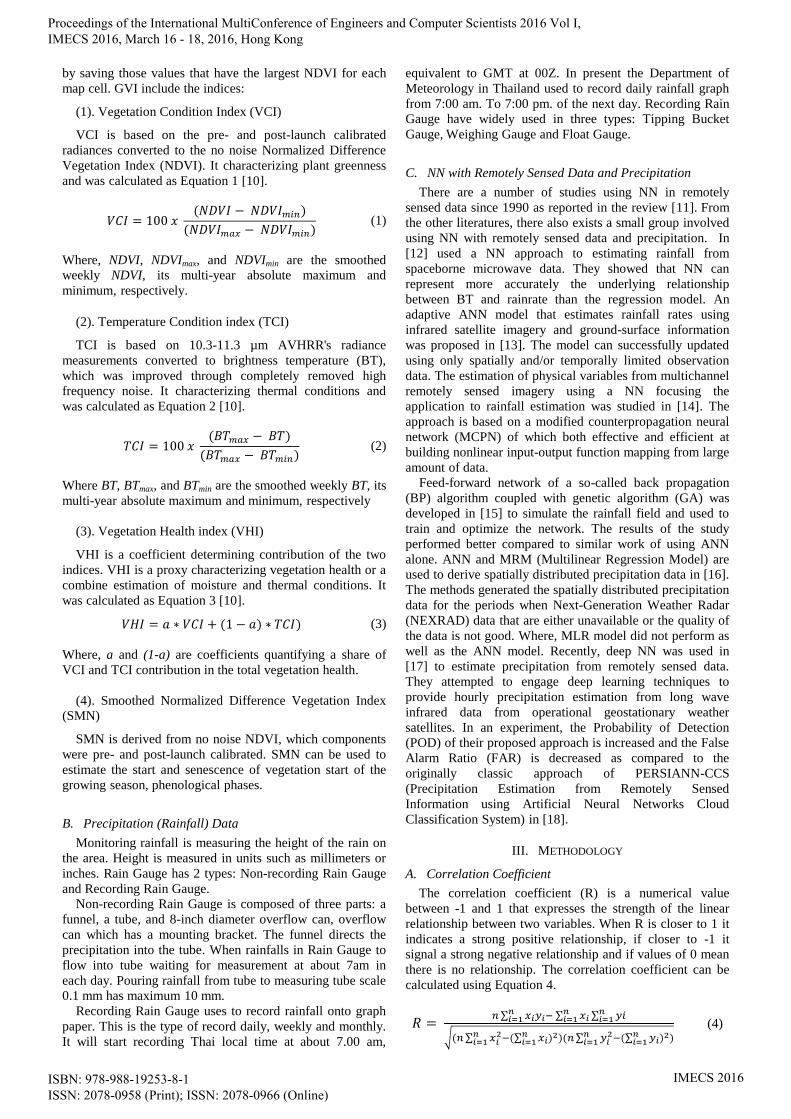
ANN consists of a set of nodes and edges between nodes

as shows in figure 1. The node has three levels: input layer,

hidden layer and output layer. Hidden layer may be more

than one layer. Nodes in the input layer called input node (or

neuron), number of nodes is equal to the number of elements

(attribute) in input data. Nodes in the hidden layer called

hidden node, number of nodes and layer are based on the

user design to experiments many different ways and use

number of node gives the best performance. The node in the

output layer called output node, number of node layer are

equal to the number of target or class to recognize in dataset.

The neural network consists of edges from all nodes in input

layer to all nodes in hidden layer and all nodes in hidden to

all nodes in output layer. ANN of at least one hidden layer

often known as Multilayer Perceptron (MLP)

Fig. 1. The architecture of the Artificial Neural Network

The process in ANN of each node can be compared to one

neuron cell in human brain. Input data is a vector of

elements: p = [p1, p2, ..., pR], R is number of elements in

input. Each input vector multiplied by weight: W = [w1, w2,

..., wR]. Then take input multiplied by the weight of each

edge. After that sum all results of each edge and bias (b).

Then forward result to transfer function, and finally can be

obtain the output.

The weight values it needs to know is important for

something we want computer to recognize. It is an uncertain

but can set computer to update weight values by learning

from the recognized pattern. If the neural network results a

false output value, the weight will be updated to the error

until it is less or obtained an acceptable.

Multilayer Perceptron (MLP) widely used the

backpropagation algorithm to adjust the weights and biases

of the network in order to minimize the mean square error.

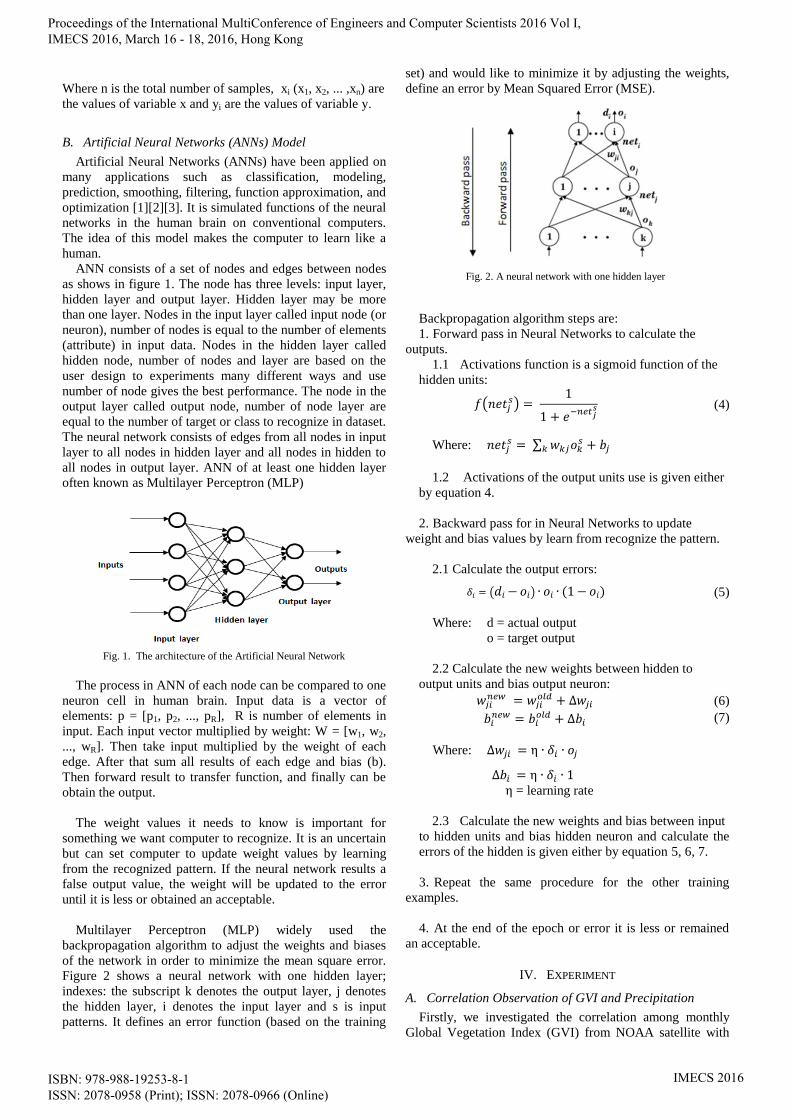
Figure 2 shows a neural network with one hidden layer;

indexes: the subscript k denotes the output layer, j denotes

the hidden layer, i denotes the input layer and s is input

patterns. It defines an error function (based on the training

set) and would like to minimize it by adjusting the weights,

define an error by Mean Squared Error (MSE).

Backpropagation algorithm steps are:

1. Forward pass in Neural Networks to calculate the

outputs.

1.1 Activations function is a sigmoid function of the

hidden units:

( )

(4)

Where: ∑

1.2 Activations of the output units use is given either

by equation 4.

2. Backward pass for in Neural Networks to update

weight and bias values by learn from recognize the pattern.

2.1 Calculate the output errors:

( ) (5)

Where: d = actual output

o = target output

2.2 Calculate the new weights between hidden to

output units and bias output neuron:

(6)

(7)

Where:

= learning rate

2.3 Calculate the new weights and bias between input

to hidden units and bias hidden neuron and calculate the

errors of the hidden is given either by equation 5, 6, 7.

3. Repeat the same procedure for the other training

examples.

4. At the end of the epoch or error it is less or remained

an acceptable.

IV. EXPERIMENT

A. Correlation Observation of GVI and Precipitation

Firstly, we investigated the correlation among monthly

Global Vegetation Index (GVI) from NOAA satellite with

Fig. 2. A neural network with one hidden layer

Proceedings of the International MultiConference of Engineers and Computer Scientists 2016 Vol I, IMECS 2016, March 16 - 18, 2016, Hong Kong

ISBN: 978-988-19253-8-1 ISSN: 2078-0958 (Print); ISSN: 2078-0966 (Online)

IMECS 2016

precipitation from ground-based rainfall measurements.

Observation GVI indices are Vegetation Health Index

(VHI), Vegetation Condition Index (VCI), Temperature

Condition Index (TCI), and Smoothed Normalized

Difference Vegetation Index (SMN). We investigated on

sample data in Nakhon Ratchasima province of Thailand

collected monthly from January 2005 to December 2014. Four

patterns of correlation between all indices and precipitation

data are examined: concurrence month, lag of one, lag of

two, and lag of three months of precipitation.

Table 1 shows pattern matching when consider the

precipitation that lag of two months. SMN index of Mar 05

will match with the precipitation back of two months, Jan

05, as indicated by an upper arrow. Therefore, the examined

correlation of the patterns of which lag of two months

considered SMN index from Mar 05 (No.3) to Dec 14

(No.120) compared to precipitation from Jan 05 (No.1) to

Oct 14 (No. 118). In the same way, lag of one month pattern

considered SMN index from Feb 05 (No.2) to Dec 14

(No.120) compared to precipitation from Jan 05 (No.1) to

Nov 14 (No. 119). And lag of three months also considered

in the same manner. Where the concurrence month, No.1 to

No. 120 of both SMN index and precipitation are matched

and compared.

Table 1. Pattern matching when considered the precipitation (RF) that

lag of two months.

No. Month SMN Index Precipitation(RF)

1 Jan 05 0.1685 0

2 Feb 05 0.1330 5.7

3 Mar 05 0.1233 20.5

4 Apr 05 0.1406 49.7

5 May 05 0.1623 193.3

6 Jun 05 0.1638 74.6

7 Jul 05 0.1764 176.9

. . . .

. . . .

. . . .

115 Jul 14 0.2171 98.7

116 Aug 14 0.2771 226

117 Sep 14 0.3488 219.9

118 Oct 14 0.3702 56.1

119 Nov 14 0.3338 13.9

120 Dec 14 0.2967 0.4

Table 2 shows the correlation coefficient among all GVI

indices with precipitation (denote by RF) of the concurrence

month. SMN index has the highest correlation with the

precipitation with coefficient value 0.1590 as indicated by

italic bold.

Table 2. Correlation coefficient among all GVI indices with

precipitation (denote by RF) of the concurrence month.

VHI VCI TCI SMN RF

VHI 1.0000 0.6596 0.7369 -0.0288 -0.0127

VCI 0.6596 1.0000 -0.0220 0.2483 0.0714

TCI 0.7369 -0.0220 1.0000 -0.2616 -0.0812

SMN -0.0288 0.2483 -0.2616 1.0000 0.1590

RF -0.0127 0.0714 -0.0812 0.1590 1.0000

Table 3 shows the correlation coefficient between each

GVI indices with precipitation that lag of 1 month, 2

months, and 3 months, respectively. All three patterns of

correlation, SMN index also has the highest correlation with

the precipitation. The degrees of relationship are much more

than the result of the concurrence month in table 2.

Especially, when the consideration precipitation is of 2

months lag as indicated by italic bold of value 0.5822. Table 3. Correlation coefficient between each GVI index with

Precipitation that lag of 1 month, 2 months, and 3 months, respectively.

VHI VCI TCI SMN RF

Lag 1 m RF -0.1526 -0.0229 -0.1766 0.5051 1.0000

Lag 2 m RF -0.2227 -0.1931 -0.1173 0.5822 1.0000 Lag 2 m RF -0.0519 -0.0735 -0.0048 0.5004 1.0000

By observation the correlation coefficient, SMN index

exposes the highest degree of relationship with precipitation

that lag of 2 months. We, consequently, use SMN index and

precipitation that lag of 2 months in analyzing with NN.

B. Experimental Setup for NN

In order to analyze the relationship between SMN index and

precipitation that lag of 2 months by NN, input and target

pairs to NN networks are matched as show in table 1. Monthly

SMN index from NOAA STAR of Nakhon ratchasima

province of Thailand collected from January 2005 to December

2014 are used as input to NN. Monthly precipitation collected

by ground-based rainfall measurements from the

Meteorological Department is considered as the target from the

same period of time. Under an assumption that current month

of SMN index will relate to the precipitation that lag of 2

months, we match each input and target pair as show by each

arrow in table 1. The first input-target pair is SMN index of

Mar 05 and precipitation of Jan 05(SMN: Mar 05, RF: Jan 05),

the second pair is SMN index of Apr 05 and precipitation of

Feb 05(SMN: Apr 05, RF: Feb 05), and so on. Therefore, input-

target pair will end by SMN index of Dec 14 and rainfall of Oct

14 (SMN: Dec 14, RF: Oct 14). As a result, we used 118

number of sample data (number of input-target pairs) to

evaluate ANN network. Where, the values of precipitation are

normalized to the interval between 0 and 1. Seventy percent of

sample data are randomly selected as the training set and the

remaining thirty percent are used for testing.

Backpropagation NN with Lavenberg-Marquardt training

algorithm (learnlm) from Matlab toolbox is used. Performances

from training and testing are evaluated in term of Mean

Squared Error (MSE) between target and output from NN.

C. Experimental Results and Discussions

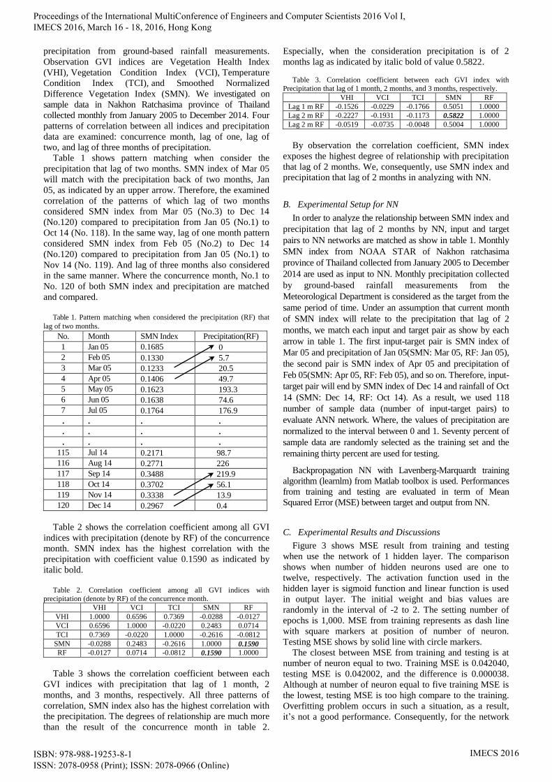
Figure 3 shows MSE result from training and testing

when use the network of 1 hidden layer. The comparison

shows when number of hidden neurons used are one to

twelve, respectively. The activation function used in the

hidden layer is sigmoid function and linear function is used

in output layer. The initial weight and bias values are

randomly in the interval of -2 to 2. The setting number of

epochs is 1,000. MSE from training represents as dash line

with square markers at position of number of neuron.

Testing MSE shows by solid line with circle markers.

The closest between MSE from training and testing is at

number of neuron equal to two. Training MSE is 0.042040,

testing MSE is 0.042002, and the difference is 0.000038.

Although at number of neuron equal to five training MSE is

the lowest, testing MSE is too high compare to the training.

Overfitting problem occurs in such a situation, as a result,

it’s not a good performance. Consequently, for the network

Proceedings of the International MultiConference of Engineers and Computer Scientists 2016 Vol I, IMECS 2016, March 16 - 18, 2016, Hong Kong

ISBN: 978-988-19253-8-1 ISSN: 2078-0958 (Print); ISSN: 2078-0966 (Online)

IMECS 2016

of 1 hidden layer using only two neurons in such layer can

get the best performance.

Fig. 3. MSE results from training and testing when use the network of 1

hidden layer. Compare when number of hidden neurons used are one to

twelve, respectively.

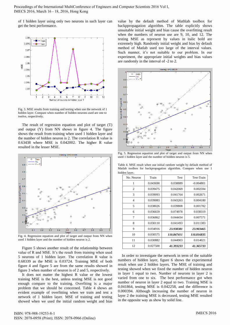
The result of regression equation and plot of target (T)

and output (Y) from NN shows in figure 4. The figure

shows the result from training when used 1 hidden layer and

the number of hidden neuron is 2. The correlation R value is

0.63438 where MSE is 0.042002. The higher R value

resulted in the lesser MSE.

Fig. 4. Regression equation and plot of target and output from NN when

used 1 hidden layer and the number of hidden neuron is 2.

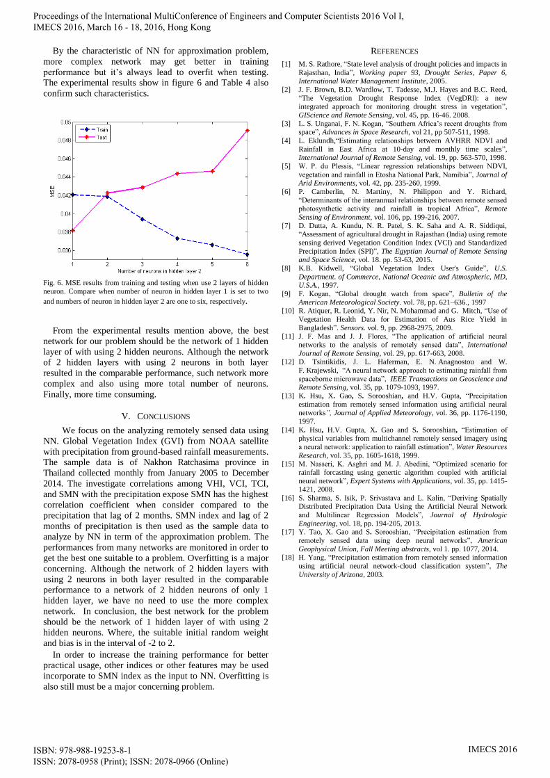
Figure 5 shows another result of the relationship between

value of R and MSE. It’s the result from training when used

5 neurons of 1 hidden layer. The correlation R value is

0.68339 as the MSE is 0.03724. Training MSE of both

figure 4 and figure 5 are from the same results showed in

figure 3 when number of neuron is of 2 and 5, respectively.

It does not matter the highest R value or the lowest

training MSE is the best, unless testing MSE is not good

enough compare to the training. Overfiting is a major

problem that we should be concerned. Table 4 shows an

evident example of overfitting when we train and test a

network of 1 hidden layer. MSE of training and testing

showed when we used the initial random weight and bias

value by the default method of Mathlab toolbox for

backppropagation algorithm. The table explicitly shows

unsuitable initial weight and bias cause the overfitting result

when the numbers of neuron use are 9, 10, and 12. The

testing MSE as represent by values in italic bold are

extremely high. Randomly initial weight and bias by default

method of Matlab used too large of the interval values.

Such manner, it’s not suitable to our problem. In our

experiment, the appropriate initial weights and bias values

are randomly in the interval of -2 to 2.

Fig. 5. Regression equation and plot of target and output from NN when

used 1 hidden layer and the number of hidden neuron is 5.

Table 4. MSE result when use initial random weight by default method of

Matlab toolbox for backpropagation algorithm. Compare when use 1

hidden layer.

No. Neuron Train Test Test-Train

1 0.043690 0.038889 -0.004801

2 0.039475 0.042069 0.002594

3 0.039093 0.041764 0.002671

4 0.039083 0.043263 0.004180

5 0.038026 0.039808 0.001782

6 0.036659 0.074978 0.038319

7 0.036862 0.044434 0.007571

8 0.030110 0.041493 0.011383

9 0.034916 23.938381 23.903465

10 0.030575 110.847411 110.816835

11 0.030882 0.044903 0.014021

12 0.027500 41.393233 41.365733

In order to investigate the network in term of the suitable

numbers of hidden layer, figure 6 shows the experimental

result when use 2 hidden layers. The MSE of training and

testing showed when we fixed the number of hidden neuron

in layer 1 equal to two. Number of neurons in layer 2 is

varied from one to six. The best performance got when

number of neuron in layer 2 equal to two. Training MSE is

0.041864, testing MSE is 0.042258, and the difference is

0.000394. Although increasing the number of neuron in

layer 2 the training MSE is decreased, testing MSE resulted

in the opposite way as show by solid line.

Proceedings of the International MultiConference of Engineers and Computer Scientists 2016 Vol I, IMECS 2016, March 16 - 18, 2016, Hong Kong

ISBN: 978-988-19253-8-1 ISSN: 2078-0958 (Print); ISSN: 2078-0966 (Online)

IMECS 2016

By the characteristic of NN for approximation problem,

more complex network may get better in training

performance but it’s always lead to overfit when testing.

The experimental results show in figure 6 and Table 4 also

confirm such characteristics.

Fig. 6. MSE results from training and testing when use 2 layers of hidden

neuron. Compare when number of neuron in hidden layer 1 is set to two

and numbers of neuron in hidden layer 2 are one to six, respectively.

From the experimental results mention above, the best

network for our problem should be the network of 1 hidden

layer of with using 2 hidden neurons. Although the network

of 2 hidden layers with using 2 neurons in both layer

resulted in the comparable performance, such network more

complex and also using more total number of neurons.

Finally, more time consuming.

V. CONCLUSIONS

We focus on the analyzing remotely sensed data using

NN. Global Vegetation Index (GVI) from NOAA satellite

with precipitation from ground-based rainfall measurements.

The sample data is of Nakhon Ratchasima province in

Thailand collected monthly from January 2005 to December

2014. The investigate correlations among VHI, VCI, TCI,

and SMN with the precipitation expose SMN has the highest

correlation coefficient when consider compared to the

precipitation that lag of 2 months. SMN index and lag of 2

months of precipitation is then used as the sample data to

analyze by NN in term of the approximation problem. The

performances from many networks are monitored in order to

get the best one suitable to a problem. Overfitting is a major

concerning. Although the network of 2 hidden layers with

using 2 neurons in both layer resulted in the comparable

performance to a network of 2 hidden neurons of only 1

hidden layer, we have no need to use the more complex

network. In conclusion, the best network for the problem

should be the network of 1 hidden layer of with using 2

hidden neurons. Where, the suitable initial random weight

and bias is in the interval of -2 to 2.

In order to increase the training performance for better

practical usage, other indices or other features may be used

incorporate to SMN index as the input to NN. Overfitting is

also still must be a major concerning problem.

REFERENCES

[1] M. S. Rathore, “State level analysis of drought policies and impacts in

Rajasthan, India”, Working paper 93, Drought Series, Paper 6, International Water Management Institute, 2005.

[2] J. F. Brown, B.D. Wardlow, T. Tadesse, M.J. Hayes and B.C. Reed,

“The Vegetation Drought Response Index (VegDRI): a new integrated approach for monitoring drought stress in vegetation”,

GIScience and Remote Sensing, vol. 45, pp. 16-46. 2008.

[3] L. S. Unganai, F. N. Kogan, “Southern Africa’s recent droughts from space”, Advances in Space Research, vol 21, pp 507-511, 1998.

[4] L. Eklundh,“Estimating relationships between AVHRR NDVI and

Rainfall in East Africa at 10-day and monthly time scales”, International Journal of Remote Sensing, vol. 19, pp. 563-570, 1998.

[5] W. P. du Plessis, “Linear regression relationships between NDVI,

vegetation and rainfall in Etosha National Park, Namibia”, Journal of Arid Environments, vol. 42, pp. 235-260, 1999.

[6] P. Camberlin, N. Martiny, N. Philippon and Y. Richard,

“Determinants of the interannual relationships between remote sensed photosynthetic activity and rainfall in tropical Africa”, Remote

Sensing of Environment, vol. 106, pp. 199-216, 2007.

[7] D. Dutta, A. Kundu, N. R. Patel, S. K. Saha and A. R. Siddiqui, “Assessment of agricultural drought in Rajasthan (India) using remote

sensing derived Vegetation Condition Index (VCI) and Standardized

Precipitation Index (SPI)”, The Egyptian Journal of Remote Sensing

and Space Science, vol. 18. pp. 53-63, 2015.

[8] K.B. Kidwell, “Global Vegetation Index User's Guide”, U.S.

Department. of Commerce, National Oceanic and Atmospheric, MD, U.S.A., 1997.

[9] F. Kogan, “Global drought watch from space”, Bulletin of the

American Meteorological Society. vol. 78, pp. 621–636., 1997 [10] R. Atiquer, R. Leonid, Y. Nir, N. Mohammad and G. Mitch, “Use of

Vegetation Health Data for Estimation of Aus Rice Yield in

Bangladesh”. Sensors. vol. 9, pp. 2968-2975, 2009. [11] J. F. Mas and J. J. Flores, “The application of artificial neural

networks to the analysis of remotely sensed data”, International

Journal of Remote Sensing, vol. 29, pp. 617-663, 2008. [12] D. Tsintikidis, J. L. Haferman, E. N. Anagnostou and W.

F. Krajewski, “A neural network approach to estimating rainfall from

spaceborne microwave data”, IEEE Transactions on Geoscience and Remote Sensing, vol. 35, pp. 1079-1093, 1997.

[13] K. Hsu, X. Gao, S. Sorooshian, and H.V. Gupta, “Precipitation

estimation from remotely sensed information using artificial neural networks”, Journal of Applied Meteorology, vol. 36, pp. 1176-1190,

1997.

[14] K. Hsu, H.V. Gupta, X. Gao and S. Sorooshian, “Estimation of

physical variables from multichannel remotely sensed imagery using

a neural network: application to rainfall estimation”, Water Resources

Research, vol. 35, pp. 1605-1618, 1999. [15] M. Nasseri, K. Asghri and M. J. Abedini, “Optimized scenario for

rainfall forcasting using genertic algorithm coupled with artificial

neural network”, Expert Systems with Applications, vol. 35, pp. 1415-1421, 2008.

[16] S. Sharma, S. Isik, P. Srivastava and L. Kalin, “Deriving Spatially Distributed Precipitation Data Using the Artificial Neural Network

and Multilinear Regression Models”, Journal of Hydrologic

Engineering, vol. 18, pp. 194-205, 2013. [17] Y. Tao, X. Gao and S. Sorooshian, “Precipitation estimation from

remotely sensed data using deep neural networks”, American

Geophysical Union, Fall Meeting abstracts, vol 1. pp. 1077, 2014. [18] H. Yang, “Precipitation estimation from remotely sensed information

using artificial neural network-cloud classification system”, The

University of Arizona, 2003.

Proceedings of the International MultiConference of Engineers and Computer Scientists 2016 Vol I, IMECS 2016, March 16 - 18, 2016, Hong Kong

ISBN: 978-988-19253-8-1 ISSN: 2078-0958 (Print); ISSN: 2078-0966 (Online)

IMECS 2016