Neuralne mreže

RadialBasisNetworks 2010

Radial basis function networks

Radial basis function network (RBFN) Hybrid network Uses the hybrid unsupervised and

supervised learning scheme The RBFN is designed to perform input-

output mapping trained by examples( ), .

Structure of the RBFN

Radial basis function networks

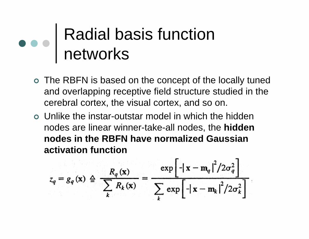
The RBFN is based on the concept of the locally tuned and overlapping receptive field structure studied in the cerebral cortex, the visual cortex, and so on.

Unlike the instar-outstar model in which the hidden nodes are linear winner-take-all nodes, the hidden nodes in the RBFN have normalized Gaussian activation function

Radial basis function networks

where is the input vector. Thus, hidden node gives a maximum response to input vectors close to .

Each hidden node is said to have its own receptive field in the input space, which is a region centered on with size proportional to where and are the mean and variance

The output of the RBFN is simply the weighted sum of the hidden node output:

Radial basis function networks

where . is the output activation function and is the threshold value.

Generally, . is an identity function (i.e., the output node is a linear unit) and 0.

The purpose of the RBFN is to pave the input space with overlapping receptive fields.

For an input vector lying somewhere in the input space, the receptive fields with centers close to it will be appreciably activated. The output of the RBFN is then the weighted sum of the activations of these receptive fields.

Radial basis function networks

In the extreme case, if lies in the center of the receptive field for hidden node , then . If we ignore the overlaps between different receptive fields, then only hidden node is activated (a winner) and the corresponding weight vector is chosen as the output, assuming linear output units.

Hence, the RBFN acts like a gradient-type forward-only counterpropagation network.

Training The RBFN is basically trained by the hybrid learning rule:

unsupervised learning in the input layer supervised learning in the output layer.

The weights in the output layer can be updated simply by using the delta learning rule:

Δ The unsupervised part of the learning involves the determination of the

receptive field centers and widths , 1, 2, … , . The proper centers can be found by unsupervised learning rules

e.g. simply the Kohonen learning rule, where is the center of the receptive field closest to the input vector and the other centers are kept unchanged.

Δ

Training

In practice, the widths are usually determined by an ad hoc choice such as the mean distance to the first few nearest neighbors (the nearest neighbors heuristic).

In the simplest case, the following first-nearest-neighbor heuristic can be used:

| |

where is the closest vector to

Advantages

The RBFN offers a viable alternative to the two-layer neural network in many applications of signal processing, pattern recognition, control, and function approximation.

In fact, it has been shown that the RBFN can fit an arbitrary function with just one hidden layer.

Also, it has been shown that a Gaussian sum density estimator can approximate any probability density function to any desired degree of accuracy.

Although the RBFN generally cannot quite achieve the accuracy of the back-propagation network, it can be trained several orders of magnitude faster than the back-propagation network. This is again due to the advantage of hybrid-learning networks which have only one layer of connections trained by supervised learning.

Supervised learning of RBFN

The RBFN can also be trained by the error back-propagation rule and becomes a purely supervised learning network.

The goal is to minimize the cost function globally

∑ ∑ = ∑ ∑ ∑

In this approach, the output layer is still trained by backpropagation.

The output error is then back-propagated to the layer of receptive fields to update their centers and widths.

Supervised learning of RBFN According to the chain rule, the supervised learning rule for

the RBFN can be derived as

In this way, the centers and widths of the receptive fields can be adjusted dynamically.

Unfortunately, the RBFN with back-propagation learning does not learn appreciably faster than the backpropagationnetwork.

Radial Basis Networks

Radial basis networks can require more neurons than standard feedforward backpropagation networks, but often they can be designed in a fraction of the time it takes to train standard feedforward networks

They work best when many training vectors are available

Two variants of radial basis networks: Generalized regression networks (GRNN) probabilistic neural networks (PNN)

Radial basis networks can be designed with either newrbe or newrb. GRNNs and PNNs can be designed with newgrnn and newpnn, respectively.

Radial Basis FunctionsNeuron Model

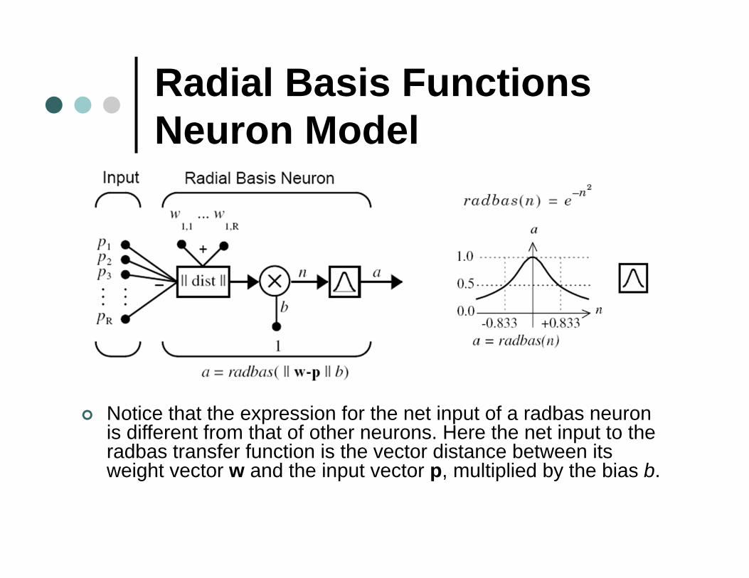
Notice that the expression for the net input of a radbas neuron is different from that of other neurons. Here the net input to the radbas transfer function is the vector distance between its weight vector w and the input vector p, multiplied by the bias b.

Network Architecture

a{1} = radbas(netprod(dist(net.IW{1,1},p),net.b{1}))

Exact Design (newrbe)

This function can produce a network with zero error on training vectors. It is called in the following way: net = newrbe(P,T,SPREAD)

This function newrbe creates as many radbas neurons as there are input vectors in P

The drawback to newrbe is that it produces a network with as many hidden neurons as there are input vectors. For this reason, newrbe does not return an acceptable solution when many input vectors are needed to properly define a network, as is typically the case

Efficient Design (newrb)

The function newrb iteratively creates a radial basis network one neuron at a time. Neurons are added to the network until the sum-squared error falls beneath an error goal or a maximum number of neurons has been reached. The call for this function is net = newrb(P,T,GOAL,SPREAD)

Radial Basis and feedforward NN

Why not always use a radial basis network instead of a standard feedforward network?

Radial basis networks, even when designed efficiently with newrbe, tend to have many times more neurons than a comparable feedforward network with tansig or logsig neurons in the hidden layer.

This is because sigmoid neurons can have outputs over a large region of the input space, while radbas neurons only respond to relatively small regions of the input space. The result is that the larger the input space (in terms of number of inputs, and the ranges those inputs vary over) the more radbas neurons required.