Radial Basis Function Network Using Orthogonal Least Squares-Genetic

Algorithm Learning (RBFN using OLSGA)

Christopher Katinas February 16, 2016

Overview • Problem Definition • Training Results • Test Results • Graphical Approximation of Results • Conclusions

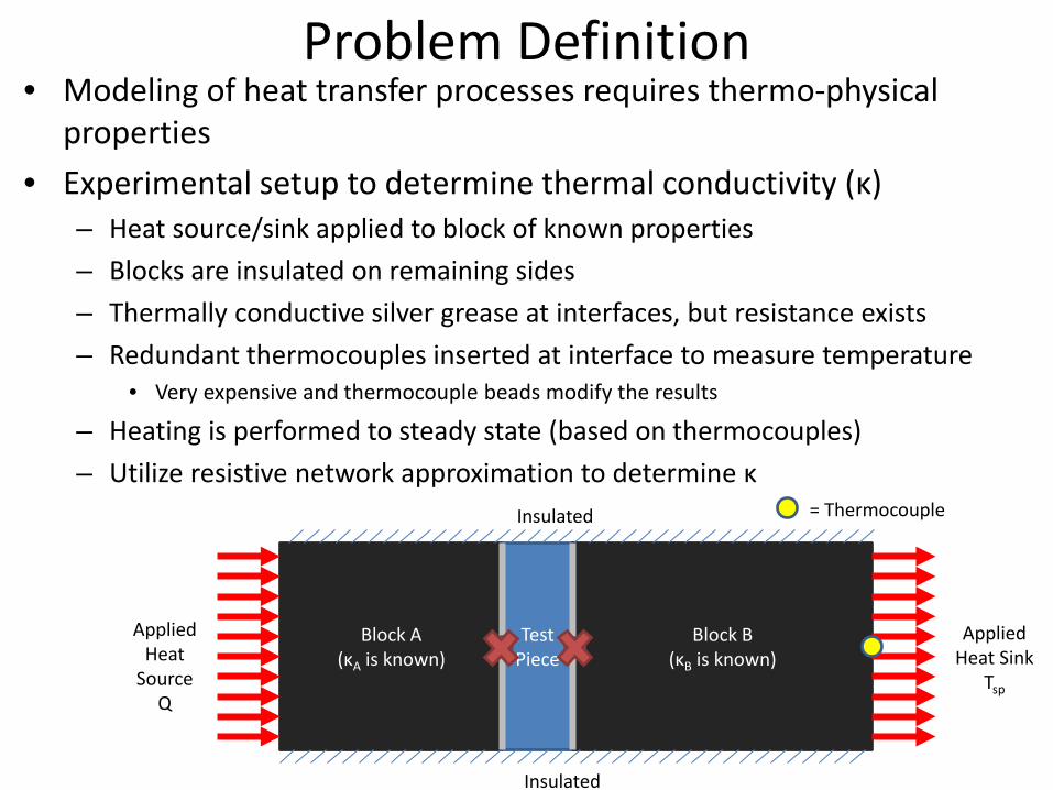
Problem Definition • Modeling of heat transfer processes requires thermo-physical

properties • Experimental setup to determine thermal conductivity (κ)

– Heat source/sink applied to block of known properties – Blocks are insulated on remaining sides – Thermally conductive silver grease at interfaces, but resistance exists – Redundant thermocouples inserted at interface to measure temperature

• Very expensive and thermocouple beads modify the results

– Heating is performed to steady state (based on thermocouples) – Utilize resistive network approximation to determine κ

Insulated

Block A (κA is known)

Test Piece

Block B (κB is known)

Insulated

Applied Heat

Source Q

= Thermocouple

Applied Heat Sink

Tsp

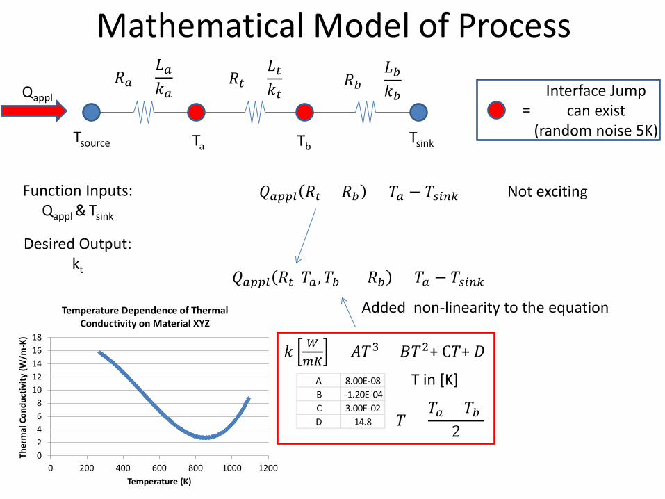
Mathematical Model of Process

02468

1012141618

0 200 400 600 800 1000 1200

Ther

mal

Con

duct

ivity

(W/m

-K)

Temperature (K)

Temperature Dependence of Thermal Conductivity on Material XYZ

𝑘𝑘 𝑊𝑊𝑚𝑚𝑚𝑚

= 𝐴𝐴𝑇𝑇3 + 𝐵𝐵𝑇𝑇2+ C𝑇𝑇+ 𝐷𝐷

A 8.00E-08B -1.20E-04C 3.00E-02D 14.8

T in [K]

Tsource

𝑅𝑅𝑎𝑎 =𝐿𝐿𝑎𝑎𝑘𝑘𝑎𝑎

Ta Tb Tsink

𝑅𝑅𝑏𝑏 =𝐿𝐿𝑏𝑏𝑘𝑘𝑏𝑏

𝑅𝑅𝑡𝑡 =𝐿𝐿𝑡𝑡𝑘𝑘𝑡𝑡

Qappl

𝑄𝑄𝑎𝑎𝑎𝑎𝑎𝑎𝑎𝑎 𝑅𝑅𝑡𝑡(𝑇𝑇𝑎𝑎 ,𝑇𝑇𝑏𝑏) + 𝑅𝑅𝑏𝑏 = 𝑇𝑇𝑎𝑎 − 𝑇𝑇𝑠𝑠𝑠𝑠𝑠𝑠𝑠𝑠

Interface Jump can exist

(random noise 5K) =

Function Inputs: Qappl & Tsink

Desired Output:

kt

Added non-linearity to the equation

𝑄𝑄𝑎𝑎𝑎𝑎𝑎𝑎𝑎𝑎 𝑅𝑅𝑡𝑡 + 𝑅𝑅𝑏𝑏 = 𝑇𝑇𝑎𝑎 − 𝑇𝑇𝑠𝑠𝑠𝑠𝑠𝑠𝑠𝑠 Not exciting

𝑇𝑇 =𝑇𝑇𝑎𝑎 + 𝑇𝑇𝑏𝑏

2

OLSGA Pseudocode 1. Create training and verification data 2. Initialize system with zero hidden nodes 3. Invoke GA & Random RBFN

a. Determine the error reduction from selected means and standard deviation (fitness function)

b. Identify mean and standard deviation with highest effect and store for future use

c. Adjust overall response vector by the projection of response vector from found parameters of GA

4. Calculate NDEI for OLSGA and Random RBFN 5. Post-process data to review RBFN function 6. Repeat steps 3-5 until maximum number of nodes is

reached (could use error tolerance, if desired)

Network Training – Heat Transfer

Lee C. W. and Shin Y. C. Growing Radial Basis Function Networks Using Genetic Algorithm and Orthogonalization. International Journal of Innovative Computing, Information and Control. 2009 Nov 1;5(11):3933-48.

• Compare NDEI trends to literature trends – Rapid decrease in NDEI when most critical nodes are found!

Trained with 2500 data points verified with 1500 points Trained with 500 data points

verified with 500 points

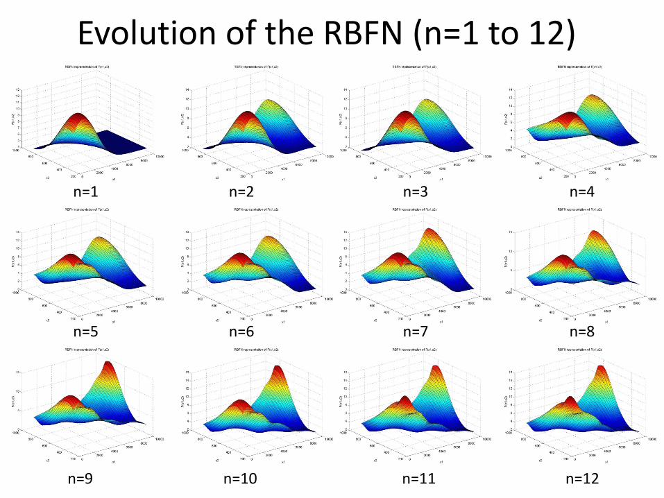
Evolution of the RBFN (n=1 to 12)

n=1 n=2 n=3 n=4

n=5 n=6 n=7 n=8

n=9 n=10 n=11 n=12

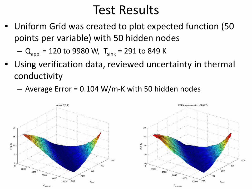
Test Results • Uniform Grid was created to plot expected function (50

points per variable) with 50 hidden nodes – Qappl = 120 to 9980 W, Tsink = 291 to 849 K

• Using verification data, reviewed uncertainty in thermal conductivity – Average Error = 0.104 W/m-K with 50 hidden nodes

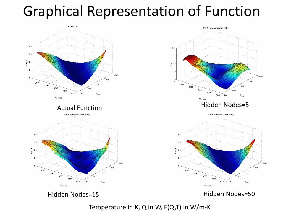
Graphical Representation of Function

Hidden Nodes=50

Hidden Nodes=5

Hidden Nodes=15

Actual Function

Temperature in K, Q in W, F(Q,T) in W/m-K

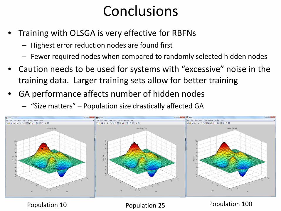
Conclusions • Training with OLSGA is very effective for RBFNs

– Highest error reduction nodes are found first – Fewer required nodes when compared to randomly selected hidden nodes

• Caution needs to be used for systems with “excessive” noise in the training data. Larger training sets allow for better training

• GA performance affects number of hidden nodes – “Size matters” – Population size drastically affected GA

Population 100 Population 10 Population 25

Extra Slides

GA Methodology • Genetic algorithm (~180 Matlab lines)

– Cross-over (0.95) • Up to three crossovers per parent pair

– Mutation Rate (0.005) – Population size/generation control – Multiple Epochs Allowed

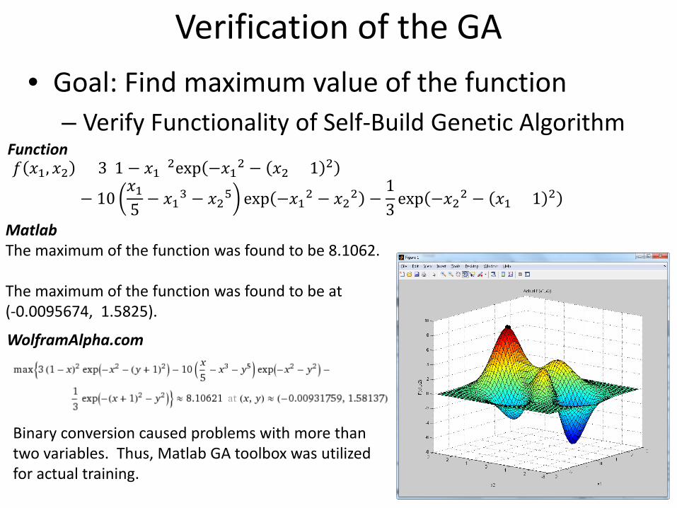
Verification of the GA

WolframAlpha.com

Matlab The maximum of the function was found to be 8.1062. The maximum of the function was found to be at (-0.0095674, 1.5825).

𝑓𝑓 𝑥𝑥1, 𝑥𝑥2 = 3(1 − 𝑥𝑥1)2exp −𝑥𝑥12 − 𝑥𝑥2 + 1 2

− 10𝑥𝑥15 − 𝑥𝑥13 − 𝑥𝑥25 exp −𝑥𝑥12 − 𝑥𝑥22 −

13

exp −𝑥𝑥22 − 𝑥𝑥1 + 1 2

Function

• Goal: Find maximum value of the function – Verify Functionality of Self-Build Genetic Algorithm

Binary conversion caused problems with more than two variables. Thus, Matlab GA toolbox was utilized for actual training.

Evolution of the RBFN for Test Function

n=1 n=2 n=3 n=4

n=5 n=6 n=7 n=8

n=9 n=10 n=11 n=12

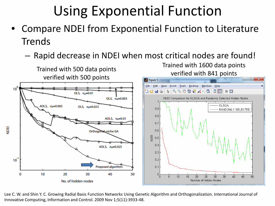
Using Exponential Function

Lee C. W. and Shin Y. C. Growing Radial Basis Function Networks Using Genetic Algorithm and Orthogonalization. International Journal of Innovative Computing, Information and Control. 2009 Nov 1;5(11):3933-48.

• Compare NDEI from Exponential Function to Literature Trends – Rapid decrease in NDEI when most critical nodes are found!

Trained with 1600 data points verified with 841 points Trained with 500 data points

verified with 500 points

Evolution of the RBFN (n=1 to 12)

n=1 n=2 n=3 n=4

n=5 n=6 n=7 n=8

n=9 n=10 n=11 n=12