Embed Size (px)
Citation preview

Laura Laitinen
Neuromagnetic sensorimotor signals in
brain computer interfaces
In partial fulfilment of the requirement for the degree of Master of Science,
Espoo 13th February 2003
Supervisor: Academy Professor Mikko Sams
Instructor: Academy Professor Mikko Sams
I
TEKNISKA HÖGSKOLAN SAMMANFATTNING AV DIPLOMARBETET
Upphovsman:
Titel:
Laura Laitinen Neuromagnetiska sensorimotoriska signaler i samband med hjärn-datorgränsnitt
Datum: 13 februari 2003 Sidantal: 77
Avdelning:
Professur:
Elektro- och telekommunikationsteknik
S-114, Kognitiv teknologi
Övervakare:
Handledare:
Akademiprofessor Mikko Sams Akademiprofessor Mikko Sams
Sammanfattning
Ett hjärn-datorgränssnitt (BCI, från engelskans Brain Computer Interface) registrerar hjärnas aktivitet och klassificerar den in i olika kategorier. Ett BCI kan användas av både förlamade och friska människor för att styra maskiner. Som input till ett BCI används vanligtvis eletroencephalografiska (EEG) signaler. Det elektriska fältet hjärnan producerar sprids då det passerar genom skallen medan det magnetiska fältet inte gör det. Därför är magnetencephalografiska (MEG) signaler mera lokaliserade än EEG signaler.
I detta arbete introduceras både hjärnforskningsmetoden MEG och arbeten som har att göra med den motoriska hjärnbarken. Teorin bakom både användingen av tid-frekvens- representationer (TFR) i samband med MEG-signalanalys och mönsteridentifikations- processer som används i BCI diskuteras.
Detta arbete evaluerar andvändingen av MEG-signaler som input till en BCI. Neuromagnetiska signalerna orsakade av både riktiga och imaginära fingerrörelser analyseras med hjälp av TFR. En expert plockar ut viktiga särdrag, så som frekvensband, från TFR-bilderna. Signalernas särdrag klassificeras sedan med hjälp av tre olika klassificerare. Både särdragen och resultaten av klassificationsprocessen rapporteras.
Resultaten visar att användingen av a priori information i klassifikationsprocessen förbättrar resultaten. Klassificeraren kunde skilja mellan rörelser av det högra och vänstra fingret hos alla fem försökspersoner. De dåliga klassificeringsresultaten från de inbildade rörelserna förbättrades genom beräknande av medeltalet av på varandra följande händelser.
Nyckelord: magnetencephalograf, hjärn-datorgränsnitt, sensorimotoriska signaler, klassificering av hjärnsignaler, tid-frekvensrepresentationer.
II
HELSINKI UNIVERSITY ABSTRACT OF THE
OF TECHNOLOGY MASTER’S THESIS
Author:
Title:
Laura Laitinen Neuromagnetic sensorimotor signals in brain computer interfaces
Date: 13th February 2003 Pages: 77
Department:
Professorship:
Department of Electrical and Communications Engineering
S-114, Cognitive Technology
Supervisor:
Instructor:
Academy Professor Mikko Sams
Academy Professor Mikko Sams
Abstract:
A brain computer interface (BCI) records the activation of the brain and classifies it into different classes. BCIs can be used by both severely motor disabled as well as healthy people to control devices. Commonly, electroencephalographic (EEG) signals produced by the brain are used as input to a BCI. The electrical field produced by the brain is distorted by the skull whereas the magnetic field is not. Consequently, EEG signals are less localised than the magnetoencephalographic (MEG) signals.
In this work, I first introduce the brain research method MEG, and then studies related to the activation of the motor cortex. The theory behind both the use of time frequency representations (TFRs) analysing MEG signals as well as the pattern recognition process used in BCIs are discussed.
This Thesis evaluates the use of MEG signals as an input to a BCI. Neuromagnetic signals caused by real and imagined finger movements are analysed using TFRs. Important features, such as frequency bands, are picked from the TFR plots by a human expert. The features in the signals are classified using three different classifiers. Both the features as well as the classification results are reported.
It is found that the use of a priori knowledge in the BCI's classification process improves the classification. The classifier was able to differentiate between left and right finger lift in all of the five subjects. The poor classification results of the imagined movements were improved by averaging over sequential trials.
Keywords: magnetoencephalography, brain computer interfaces, sensorimotor signals, classification of brain signals, time-frequency representations.

III
To my mother and father

IV
Foreword
This work was done in the Laboratory of Computational Engineering (LCE) at the
Helsinki University of Technology (HUT). LCE was selected as the Academy of
Finland’s centre of excellence for years 2000-2005. This Thesis is part of the
research done in the group of Cognitive Science and Technology’s brain computer
interface project. The supervisor and instructor was Academy Professor Mikko
Sams.
I would like to express my deepest appreciation for the help and dedication
Academy Professor Mikko Sams has given for this work. Our long discussions on
scientific work will be remembered. Additionally, I would like to thank Academy
Professor Riitta Hari for her valuable comments. I would also like to thank M. Sc.
Tommi Nykopp for everything he has taught me about classifying brain signals. In
addition, I would like to thank M. Sc. Toni Auranen and M. Sc. Riikka Möttönen for
their eagerness to help whenever I needed it.
Furthermore, I would like to thank my family and friends for supporting me during
these last six months. I would especially like to thank my father for both the
encouragement and help he has given during the writing process. Finally, I would
like to express my gratitude to my beloved partner Antti for helping me in all
possible ways. I could not have done it without his support.
In Espoo, 13th February, 2003
Laura Laitinen

V
Contents
1 Introduction..........................................................................................................1
1.1 General introduction ........................................................................................ 1
1.2 Magnetoencephalography (MEG) ................................................................... 3
1.2.1 Neuronal currents..................................................................................... 3
1.2.2 The forward and inverse problem............................................................ 5
1.2.3 Instrumentation ........................................................................................ 8
1.2.4 Magnetoencephalography compared with electroencephalography...... 10
1.3 Studies on the sensorimotor cortex ................................................................ 11
1.3.1 Anatomy................................................................................................. 11
1.3.2 The rhythmic activity of the cortex........................................................ 13
1.3.3 Motor imagery ....................................................................................... 17
1.3.4 The activation of the sensorimotor cortex in paralysed patients............ 19
1.4 Studying brain activation ............................................................................... 21
1.4.1 Time domain analysis and event-related responses ............................... 21
1.4.2 Frequency-domain analysis ................................................................... 22
1.4.3 Time-frequency representation and wavelets ........................................ 24
1.4.4 Neural networks used for pattern recognition........................................ 26
1.5 Brain computer interfaces .............................................................................. 33
1.5.1 Definition of a brain computer interface................................................ 33
1.5.2 Brain interfaces based on electroencephalography................................ 34
1.5.3 Brain computer interfaces used with other recording techniques.......... 36
2 Method ...............................................................................................................38
2.1 Subjects and procedure .................................................................................. 38
2.1.1 Experimental procedure ......................................................................... 38
2.1.2 Data acquisition ..................................................................................... 39
2.2 Time-frequency representations..................................................................... 40

VI
2.2.1 The calculation of the time-frequency representations.......................... 40
2.3 Pattern recognition and classification ............................................................ 42
2.3.1 Preprocessing and baselining................................................................. 42
2.3.2 Feature extraction................................................................................... 45
2.3.3 Feature classification ............................................................................. 46
2.3.4 Averaging sequential trials ...................................................................... 47
3 Results................................................................................................................48
3.1 The features.................................................................................................... 48
3.1.1 Right and left finger movement ............................................................. 51
3.1.2 Imagined right and left finger movement .............................................. 54
3.2 Classification results ...................................................................................... 56
3.2.1 Right vs. left finger movement .............................................................. 56
3.2.2 Imagined right vs. left finger movement................................................ 57
3.2.3 Channel capacity.................................................................................... 59
3.3 The effect of averaging .................................................................................. 60
4 Discussion..........................................................................................................65
Appendix A................................................................................................................70
References..................................................................................................................72
VII
List of figures
Figure 1.1: A model of the current flow of an excitatory post synaptic neuron.…….5
Figure 1.2 The VectorviewTM device.………………………….…..………………..9
Figure 1.3: Two different gradiometers on top of the magnetic field pattern produced
by a dipole. …………………………………………………………………………9
Figure 1.4: Right lateral view of the right cerebral hemisphere……………………12
Figure 1.5: The three different areas of the somatosensory cortex…………………13
Figure 1.6: The somatotopic organisation of the motor cortex..……………………14
Figure 1.7: The ERD/ERS of the motor cortex during right finger movements..…16
Figure 1.8: Grand average ERD/ERS during motor imagery..……………………19
Figure 1.9: The movement related evoked magnetic fields as a function of time.…22
Figure 1.10: The different steps of the TSE analysis..……………………………24
Figure 1.11: The frequency resolution of the Fourier and wavelet transform..…….25
Figure 1.12: The pattern recognition process used in biomedical signal analyses...27
Figure 1.13: Decision boundary for ANN classifiers..…………………………….28
Figure 1.14: A feed forward multi layer perceptron..…………………………….29
Figure 1.15: A single layer network diagram………………………………………30
Figure 1.16: An example of a confusion matrix with three classes………………32
Figure 1.17: Subject using the virtual keyboard application of ABI………………35
Figure 2.1: Schematic drawing of the stimulus sequence of one trial……………39
Figure 2.2:The TFR of one MEG sensor………………………………….……... 40
VIII
Figure 2.3: TFRs of 102 sensor places……………………………………………...41
Figure 2.4: The effect of baseline…………………………………………………...44
Figure 2.5: Feature space……………………………………………………………47
Figure 3.1: Step one in the feature extraction process……………………………...48
Figure 3.2: Step two and three in the feature extraction process…………………...49
Figure 3.3: Step two and three in feature extraction process for the imagined
movements………………………………………………………………………….50
Figure 3.4: The activation during right finger movement…………………………..52
Figure 3.5: The activation during left finger movement……………………………52
Figure 3.6: The activation during the neutral condition………………………….…53
Figure 3.7: The statistical significance of the right vs. left lift condition…………..53
Figure 3.8: The activation during imagination of right finger movement……..……55
Figure 3.9: The activation during imagination of left finger movement……………55
Figure 3.10: The effect of averaging on subject S1……………………………...…60
Figure 3.11: The effect of averaging on all subjects during right finger
movements…………………………………………………………………………..61
Figure 3.12 The effect of averaging in feature space……………………………….62
Figure 3.13: The effect of averaging on the classification results of real
movements…………………………………………………………………………..63
Figure 3.14: The channel capacity of real movements……………………………...63
Figure 3.15: The effect of averaging on the classification results of imagined
movements…………………………………………………………………………. 64
IX
List of tables
Table 3.1: The real movement feature components……………………………....51
Table 3.2: The features for the imagined movements……………………………54
Table 3.3:The classification results of the RBF classifier……………………….56
Table 3.4: Parameters for the real movement condition…………………………57
Table 3.5: The classification results for the imagined movements………………58
Table 3.6: Parameters for the imagined movement condition……………………58
Table 3.7: The average performance of the three classifiers……………………59
Table 3.8: The channel capacities of each subject…………………………………59
X
Abbreviations
ABI Adaptive Brain Interface
ANN Artificial neural network
AR Auto-regressive
BCI Brain computer interface
DFT Discrete Fourier transform
ECD Equivalent current dipole
EEG Electroencephalography
EMG Electromyography
EOG Electro-oculogram
EPSP Excitatory postsynaptic potential
ERD Event-related desynchronization
ERF Event-related field
ERP Event-related potential
ERR Event-related response
ERS Event-related synchronization
FFT Fast Fourier transform
fMRI Functional magnetic resonance imaging
HPI Head position indicator
HUT Helsinki University of Technology
KNN K-nearest neighbors classifier
LCE Laboratory of Computational Engineering
M20 ERF component 20 ms after an event has occurred
MEF Movement evoked field
MEG Magnetoencephalography
MF Motor field
MLP Multi-layer perceptron
MRI Magnetic resonance imaging
N100 Negative peak in the ERP 100ms after an event has occurred
PET Positron emission tomography
P300 Positive peak in the ERP 300 ms after an event occurred
XI
PSP Postsynaptic potential
RBF Radial basis function
RF Readiness field
SI Primary somatosensory cortex
SII Secondary somatosensory cortex
SEF Somatosensory evoked magnetic field
SNR Signal to noise ratio
SQUID Super conducting quantum interference device
SSP Signal-space projection
STFT Short term Fourier transform
TFR Time frequency representation
TSE Temporal spectral evolution
VEP Visual evoked potential

XII
Symbols
a Dyadic scale of a basis function
b Dyadic translation of a basis function
bi The output of the ith gradiometer
B Magnetic field strength
dk The error of the delta learning rule of an artificial neural network
E Electrical field strength
∂o Permitivity of free space
f Frequency
J Current density vector
tJ Total current
JP Primary current
Jv Volume current
K+ Potassium ion
Li Lead field
Na+ Sodium ion
r Charge density
s(r) Macroscopic conductivity
m0 Permeability of free space
x. Input vector to an ANN
X(f) Signal in frequency domain
x(t) Signal in time domain
y Output vector of an ANN
w Weight vector of an artificial neural network
w The width of the Morlet wavelet

1
1 Introduction
1.1 General introduction
Every movement, perception and thought we perform is associated with distinct neural
activation patterns. Neurons in the brain communicate with each other by sending
electrical impulses that produce currents. These currents give rise to both a magnetic
and electrical fields that can be measured outside the head. A brain computer interface
(BCI) records the signals produced by the brain picks out specific patterns from these
signals and classifies these patterns into different categories. The classifier attempts to
differentiate the brain signal produced by one action from those produced by other
actions. The categories can be associated with simple computer commands and the BCI
can be used to operate, e.g., a virtual keyboard.
The electroencephalographic (EEG) and magnetoencephalographic (MEG) signals
measured from head surface are a sum of all the momentary brain activation. It is
difficult to distinguish the patterns correlated with a certain event from these signals.
Furthermore, the BCI has to detect instantly the activation related to an event based on
single trials, which makes the recognition problem even more difficult. Most present
noninvasive BCIs are based on EEG signals (Volpaw et. al., 2002). The concentric
inhomogeneities of the tissue distort the electrical fields. Because the tissue does not
affect the magnetic fields, the spatial accuracy of MEG is better than that of EEG. On
the other hand, in the case of an ideal sphere, MEG does not detect the radial current
sources whereas EEG does. Both techniques have their advantages and disadvantages.
The sensorimotor cortex of humans has been extensively studied. Activation related to
hand movements is localised on both sides of the sensorimotor cortices. Furthermore,
the activation patterns are mainly contralateral. The activation patterns during
2
imagination of hand movements resemble the activation patterns during preparation of
hand movements (Jeannerod (1994)).
We are developing a BCI based on simultaneous recordings of MEG and EEG. To
begin with, we aim at constructing a very robust BCI based on brain activity related to
real movements. The use of imagined movements will also be investigated. The long-
term aim is to determine the limits of noninvasive BCIs.
The aim of this Thesis is to study the use of MEG signals in BCIs.
MEG signals during finger lifting were inspected. The brain signals were analysed off
line using time frequency representations (TFRs). The objective was to study the TFRs
to select the best possible features for the BCI classifier. In addition, the brain's
activation during the real and imagined movements was compared.
Chapter 1 provides a literature review related to the neuromagnetic activation of the
brain and its relation to BCIs. The literature review is divided into four main sections.
The first section deals with the instrumentation used to study neuromagnetic signals
and the currents that generate these signals. The section ends with an outline on the
differences between MEG and EEG.
The second section provides a review of functions of the sensorimotor cortex. The
anatomy as well as the activity of the sensorimotor cortex during real and imagined
movements is discussed. Studies on the activation of the cortex in paralysed patients.
Section three discusses the analysis methods of MEG signals. Signals can either be
analysed in time or in frequency domain. To take advantage of both the time and
frequency information, the signals can also be analysed using time-frequency
representations. Finally the signals can also be inspected and pattern recognition of the
signals can be implemented using mathematical models, such as artificial neural
networks. The fourth section defines a BCI and reviews BCI research. Both EEG-based
and invasive BCIs are discussed.
Chapter two contains the material and method section. The results are presented in
Chapter three. Chapter four discusses the results of the study.

3
1.2 Magnetoencephalography (MEG)
1.2.1 Neuronal currents
The human brain is mainly built of neurons and glial cells. The glial cells keep the
chemical environment stable and transport nutrition and waste material. The neurons
are specialised in processing information, with the help of electrical impulses called
action potentials and so called postsynaptic potentials. A neuron can be divided into
three major parts, its cell body (soma), an axon and several dendrites. Through the
synapses, the dendrites receive excitation from other neurons and conduct it to the soma
and axon. The axon transports the impulse to another synapse. Glial cells called
oligodendrocytes surround the neurons, forming an insulating myelin sheath that leaves
only small parts of the axon free, the nodes of Ranvier, and thus speeding up the course
of the action potentials (for review, see Hyvärinen, 1977).
During resting condition, the extracellular compartment of the axon is rich in sodium
(Na+) ions while the intracellular solution is rich of potassium (K+) ions (Glaser, 2001).
The cell membrane’s permeability to potassium dominates that of sodium. As a result
the inside of the cell membrane becomes more negative as the potassium ions diffuse
out of the cell.
The sodium, potassium and other ions create an electrical current by moving across the
cell membrane of an axon. If the voltage at the axon hillock, which is situated between
the axon and the soma, reaches the firing threshold, the voltage-gated sodium channels
react and sodium flows into the first part of the axon. The membrane potential grows to
about +30 mV (Kandel et al., 1991). The change of potential triggers the neighbouring
area, making the action potential move without energy consumption through the axon.
After reaching a certain voltage, the potassium channels open and potassium ions flow
out of the cell, returning the axon back to its resting potential. To restore the original
situation, Na+-K+ pumps drives the Na+ ions out of the cell and the K+ ions back into
the cell with the help of energy.
4
At the end of the axon there is a synapse (connection) to another cell’s dendrite or
soma. The impulses are mediated from one cell to another either through an electrical
synapse or chemical synapse. In a chemical synapse, synaptic vesicles in the axon of
the presynaptic cell let neurotransmitters free into the liquid between the cells. As the
neurotransmitters reach the postsynaptic cell, they can either open up sodium or
chloride channels resulting in a potential difference over the membrane. The former is
called an excitatory postsynaptic potential (EPSP) and the latter an inhibitory PSP
(Kandel et al., 1991). A single excitatory PSP increases the cell membrane potential
only a couple of millivolts and several excitatory PSPs have to occur before an action
potential is fired (Hyvärinen, 1977).
The amplitude of an action potential always remains the same. When the excitatory
input becomes stronger, only the firing frequency of the neuron increases. Action
potentials last only about 1 ms whereas synaptic currents can have duration of tens of
milliseconds (Kandel et al., 1991).
Modelling currents of the brain
As the neurotransmitters reach the dendrite in an EPSP, this part of the cell becomes
depolarised. The current flows through the dendrite to the soma creating a current sink
at the end of dendrite and a current source by the soma. (Clark, 1995). The synaptic
current flow can be modelled as a current dipole and the action potential by two
oppositely oriented current dipoles, a quadrupole. The dipolar field of a quadrupole
decreases with distance (r) as 1/r3 and a dipole as 1/r2 (Hämäläinen et al, 1993).
Because of the greater attenuation of the quadrupoles, the measured magnetic field
signal is mainly produced by the EPSP Hämäläinen et al. (1993) The currents
associated with the PSP can be divided into two components, the primary current Jp and
the volume current Jv . The volume current is also known as either the secondary or the
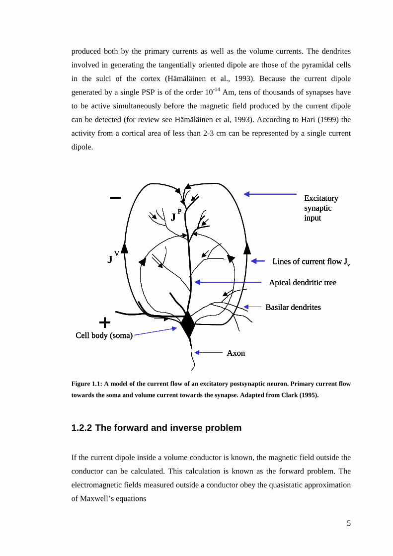
return current. Fig. 1.1 shows a model of the postsynaptic current in a neuron and how
the different currents flow. The volume current is a result of the macroscopic electric
field and is a passive current. The total current is defined as
EJJJJ PVP σ+=+= (1.1)
where J and E are the current density and the electrical field and s is the macroscopic
conductivity (see e.g. Hämäläinen et al., 1993). The measured magnetic field is
5
produced both by the primary currents as well as the volume currents. The dendrites
involved in generating the tangentially oriented dipole are those of the pyramidal cells
in the sulci of the cortex (Hämäläinen et al., 1993). Because the current dipole
generated by a single PSP is of the order 10-14 Am, tens of thousands of synapses have
to be active simultaneously before the magnetic field produced by the current dipole
can be detected (for review see Hämäläinen et al, 1993). According to Hari (1999) the
activity from a cortical area of less than 2-3 cm can be represented by a single current
dipole.
Excitatory synaptic input
Lines of current flow Jv
Basilar dendrites
Axon
Cell body (soma)
Apical dendritic tree
JP
JV
Excitatory synaptic input
Lines of current flow Jv
Basilar dendrites
Axon
Cell body (soma)
Apical dendritic tree
Excitatory synaptic input
Lines of current flow Jv
Basilar dendrites
Axon
Cell body (soma)
Apical dendritic tree
JP
JP
JV
JV
Figure 1.1: A model of the current flow of an excitatory postsynaptic neuron. Primary current flow
towards the soma and volume current towards the synapse. Adapted from Clark (1995).
1.2.2 The forward and inverse problem
If the current dipole inside a volume conductor is known, the magnetic field outside the
conductor can be calculated. This calculation is known as the forward problem. The
electromagnetic fields measured outside a conductor obey the quasistatic approximation
of Maxwell’s equations

6
tJB
B
E
E
0
0
0
0
/
µ
ερ
=×∇
=⋅∇=×∇
=⋅∇
(1.2)
where E and B are the electrical field strength and magnetic flux density and, tJ and r
are the total current and the charge density, and ∂o and mo are the permittivity and
permeability of free space. The quasistatic approximation can be made because the
frequency of bioelectrical signals is below 1 kHz (Hämäläinen et al., 1993).
The total magnetic field outside a volume conductor generated by a primary current
distribution inside the volume conductor can be calculated with the Ampere-Laplace
law
∫ −
−×= ''
)'()'(
4)( 3
0 dvrr
rrrJrB
πµ
(1.3)
where r is the point where the field is computed and r ’ is the location of the source.
The total current density )'(rJ is divided into two components given by equation (1.1)
(Hämäläinen et al., 1993). In order to solve (1.3), the volume currents needs to be
calculated first. Here some assumptions have to be made about the conductivity of the
head. There are several special cases to the forward problem. The most commonly used
model for the volume conductor is an spherically symmetric conductor. This model
works well in most areas of the head as long as the radius of the sphere is fitted to the
local radius of curvature of the measurement (Hari and Ilmoniemi, 1986). In the
spherical model, only tangential components of the currents produce magnetic fields
outside the head (Hari, 1999). Sometimes it is appropriate to model the human head
using a realistic head model. However, in this case it is sufficient to model only the
space inside the poorly conducting skull because only a small proportion of the currents
flow in the skull.
The inverse problem
Magnetoencephalography measures the magnetic field outside the head surface. Let us
assume that the conductivity of the head is known or that we have estimated it with a
7
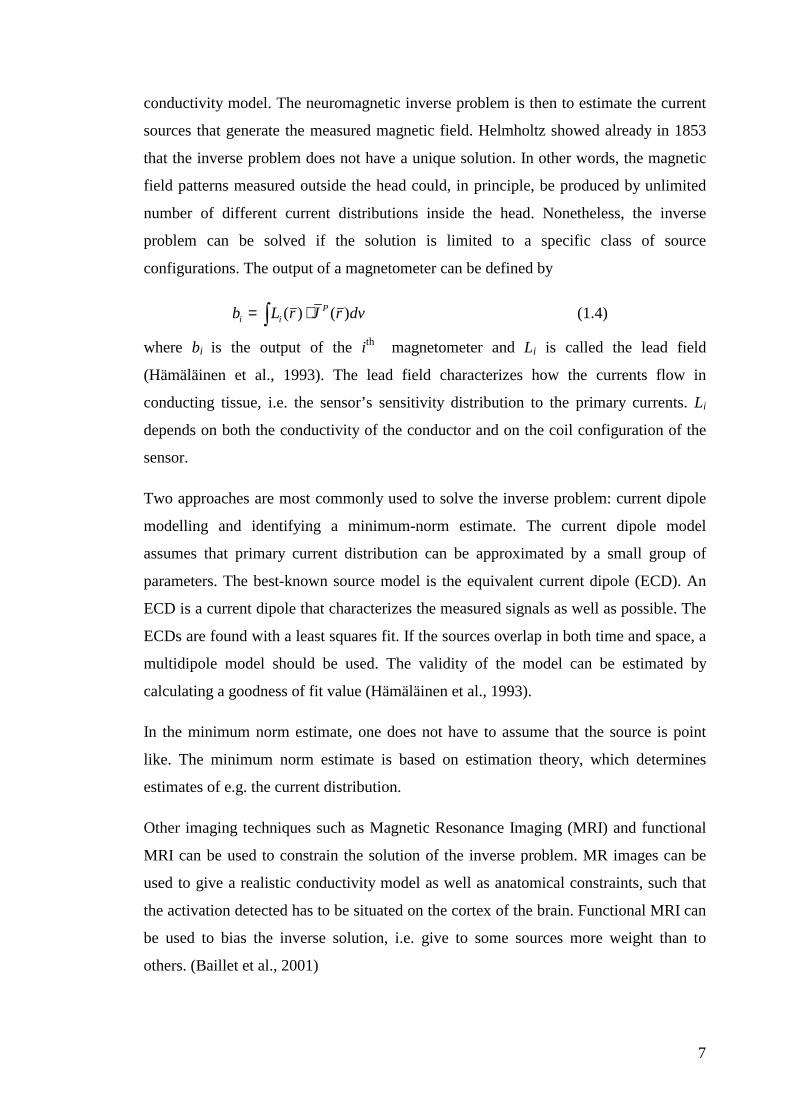
conductivity model. The neuromagnetic inverse problem is then to estimate the current
sources that generate the measured magnetic field. Helmholtz showed already in 1853
that the inverse problem does not have a unique solution. In other words, the magnetic
field patterns measured outside the head could, in principle, be produced by unlimited
number of different current distributions inside the head. Nonetheless, the inverse
problem can be solved if the solution is limited to a specific class of source
configurations. The output of a magnetometer can be defined by
dvrJrLb Pii )()( ⋅= ∫ (1.4)
where bi is the output of the ith magnetometer and Li is called the lead field
(Hämäläinen et al., 1993). The lead field characterizes how the currents flow in
conducting tissue, i.e. the sensor’s sensitivity distribution to the primary currents. Li
depends on both the conductivity of the conductor and on the coil configuration of the
sensor.
Two approaches are most commonly used to solve the inverse problem: current dipole
modelling and identifying a minimum-norm estimate. The current dipole model
assumes that primary current distribution can be approximated by a small group of
parameters. The best-known source model is the equivalent current dipole (ECD). An
ECD is a current dipole that characterizes the measured signals as well as possible. The
ECDs are found with a least squares fit. If the sources overlap in both time and space, a
multidipole model should be used. The validity of the model can be estimated by
calculating a goodness of fit value (Hämäläinen et al., 1993).
In the minimum norm estimate, one does not have to assume that the source is point
like. The minimum norm estimate is based on estimation theory, which determines
estimates of e.g. the current distribution.
Other imaging techniques such as Magnetic Resonance Imaging (MRI) and functional
MRI can be used to constrain the solution of the inverse problem. MR images can be
used to give a realistic conductivity model as well as anatomical constraints, such that
the activation detected has to be situated on the cortex of the brain. Functional MRI can
be used to bias the inverse solution, i.e. give to some sources more weight than to
others. (Baillet et al., 2001)
8
The inverse solution does not take into account the silent sources in the head.
Magnetically silent sources are e.g. a radially orientated current dipoles in a spherical
conductor. Because of the non-uniqueness of the inverse solution it is important to bear
in mind that one inverse solution is not necessarily better than another. Without prior
knowledge, one cannot know what the best inverse solution might in this case be.
1.2.3 Instrumentation
The magnetic field produced by the brain is a 109-108’s part of the geomagnetic field
(Hämäläinen et al., 1993). This is why most MEG measurements are conducted inside a
magnetically shielded room. The shielded room at the Low Temperature Laboratory at
the Helsinki University of Technology is made of several layers of aluminium and mu-
metal (Hari, 1999). Currently most MEG instruments are based on Superconducting
Quantum Interferences Devices (SQUIDs) that allow recordings of very small
biomagnetic fields. The SQUID consists of a superconducting loop. In the mostly
commonly used dc-SQUID, two Josephson junctions that are characterised by a critical
current Ic interrupt the loop. The ring becomes resistive, if a larger amount of current is
passed through the ring than Ic. Current is induced into the ring by a magnetic flux
(Hämäläinen et al., 1993). A flux transformer is a device used to bring the magnetic
signal to the SQUID. The SQUIDs have to be immersed in liquid helium (at –269± C)
to keep the superconductivity. The liquid helium is kept in a dewar container that has to
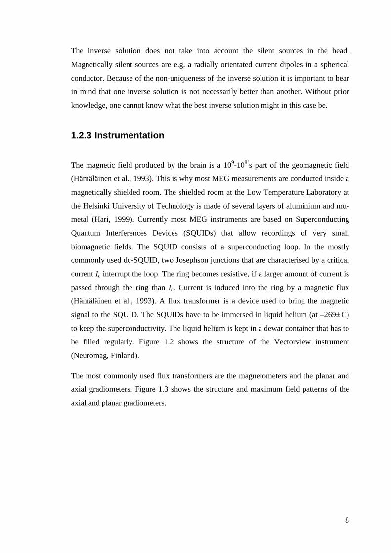
be filled regularly. Figure 1.2 shows the structure of the Vectorview instrument
(Neuromag, Finland).
The most commonly used flux transformers are the magnetometers and the planar and
axial gradiometers. Figure 1.3 shows the structure and maximum field patterns of the
axial and planar gradiometers.
9
Figure 1.2: The VectorviewTM device. The figure also shows where the flux transformers and the
dewar are situated. The figure on the left shows the positions of the triple sensor units. Modified
from Neuromag system hardware description (2000).
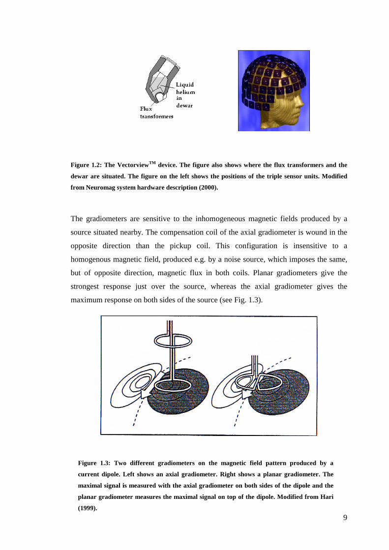
The gradiometers are sensitive to the inhomogeneous magnetic fields produced by a
source situated nearby. The compensation coil of the axial gradiometer is wound in the
opposite direction than the pickup coil. This configuration is insensitive to a
homogenous magnetic field, produced e.g. by a noise source, which imposes the same,
but of opposite direction, magnetic flux in both coils. Planar gradiometers give the
strongest response just over the source, whereas the axial gradiometer gives the
maximum response on both sides of the source (see Fig. 1.3).
Figure 1.3: Two different gradiometers on the magnetic field pattern produced by a
current dipole. Left shows an axial gradiometer. Right shows a planar gradiometer. The
maximal signal is measured with the axial gradiometer on both sides of the dipole and the
planar gradiometer measures the maximal signal on top of the dipole. Modified from Hari
(1999).

10
1.2.4 Magnetoencephalography compared with
electroencephalography
Electroencephalography means the registration of the electrical activity of the brain.
EEG is closely related to MEG. However, there are some differences. First, the primary
currents causing both the magnetic fields as well as the electrical fields are the same,
except that MEG and EEG measure different components of it. EEG is sensitive to both
the tangential and radial component of the primary current, whereas MEG is sensitive
only to the tangential component (Hämäläinen et al., 1993).
Secondly, EEG has poorer spatial accuracy than MEG because in general the skull and
other extra-cerebral tissues distort the electrical field but not the magnetic fields. More
precise knowledge of the conductivities of the tissues in the head is needed in the
interpretation of the EEG signals than in the interpretation of the MEG signals. MEG
signals are easier to interpret than EEG signals.
Thirdly, EEG is the registration of the potential difference between scalp electrodes.
These registrations are always bipolar. Even when the electrodes are referred to a
distant reference electrode, the measurements are bipolar, because there is no such
thing as an inactive reference. The MEG measurements are reference-free.
In addition, the instrumentation used to measure MEG signals is much more expensive
than the EEG equipment. Even though MEG and EEG signals should be measured in
shielded rooms, EEG is less sensitive to noise and can be obtained outside a shielded
room as well. The MEG SQUIDs have to be kept at a low temperature, which makes
the MEG device rather immobile. EEG electronics in contrast can be made really small
and several different portable EEG systems are available on the market (see e.g. Yuasa
et al., 2001).
EEG picks up some current sources better than MEG. These include e.g. sources that
are very deep and radial. On the other hand, MEG is more precise at detecting the
tangential components of the sources than EEG. To obtain comprehensive information
on the primary currents generated by brain activity, one should take into account both
11
the information provided by EEG and MEG. In the optimal case, these two imaging
techniques should be recorded simultaneously.
1.3 Studies on the sensorimotor cortex
1.3.1 Anatomy
The human brain, the cerebrum, is a part of the central nervous system and it is divided
by the longitudinal fissure into a left and right cerebral hemisphere. Most of the
connections between the hemispheres go through the corpus callosum. Both
hemispheres consist of four lobes, frontal, parietal, occipital and temporal (see Fig.
1.4). Each hemisphere relates principally to the opposite side of the body. The cerebral
cortex is a thin layer of grey matter, i.e. cell bodies, covering the outer surface of the
cerebrum. Different areas of the cortex care specialised for to different functions, for
example the posterior part is known as the visual cortex (Hyvärinen, 1977).
The sensorimotor cortex, also known as the Rolandic cortex, consists of both the motor
cortex and the somatosensory cortex. The primary motor cortex is located anterior of
the central sulcus and the somatosensory cortex is situated posterior of it.
The motor cortex is divided into two cytoarhitectonic areas, 4 and 6. Area 4 is known
as the primary motor cortex whereas area 6 is known as the supplementary motor area
(Rizzolatti and Luppino, 2001). The motor cortex also consists of a more loosely
defined premotor area (Geyer et al., 2000). Animal studies as well as functional studies
of the human brain have, however, shown that this division of the motor cortex is too
simplistic. A mosaic of anatomically and functionally distinct areas formats the motor
cortex of humans. Each of these areas manage different aspects of motor behaviour

12
Figure 1.4: Right lateral view of the right cerebral hemisphere. The four lobes of the cortex are
marked as well as the locations of motor cortex and the somatosensory cortex. Moore and Dalley
(1999).
The primary motor cortex is organised somatotopically so that different parts of it
control different parts of the body. Each part of the body is represented in the brain in
proportion to its relative importance in motor behaviour. Body parts that are used for
complicated movements such as the hands are represented by larger areas in the
primary motor cortex (see Fig. 1.6). The non-primary motor areas are mostly involved
in the preparation of voluntary movements (Geyer et al., 2000).
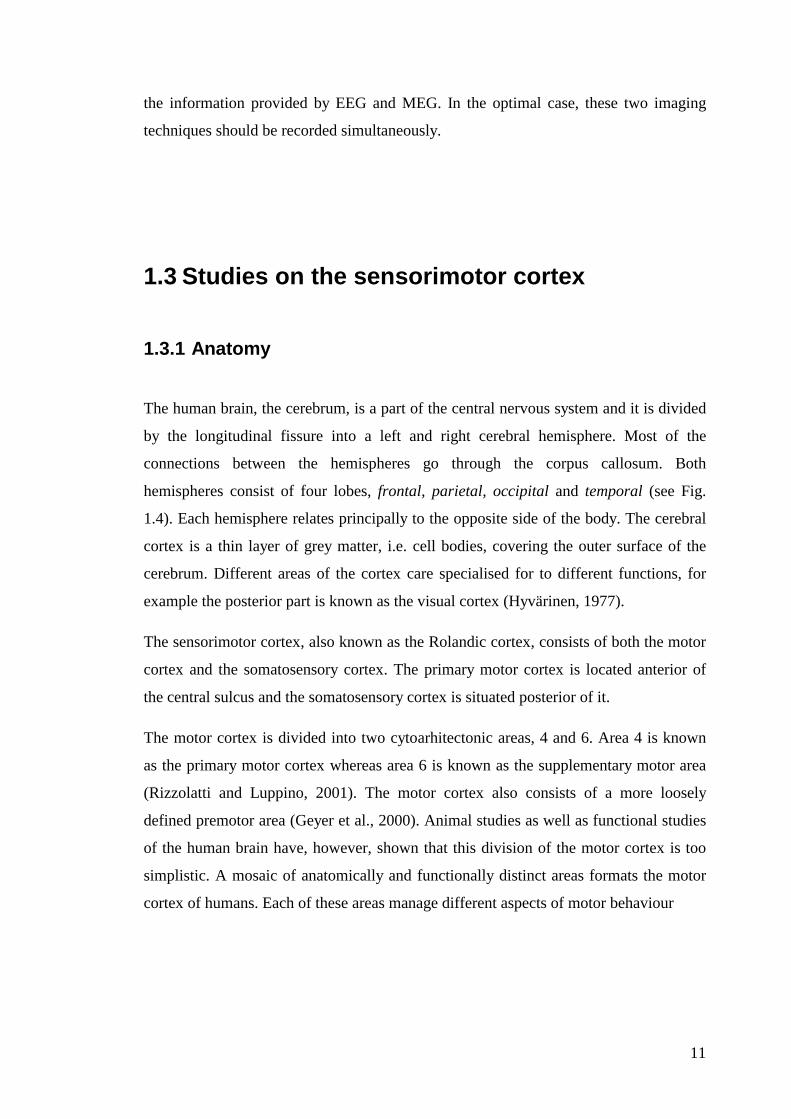
The somatosensory cortex collects sensory information from the body. It consists of a
primary somatosensory cortex (SI) and a secondary somatosensory cortex (SII) (see
Fig. 1.5). SI consists of four different cytoarhitectonic regions, each of these displays a
clear somatotopic organization. SII shows also roughly a somatotopic organization but
its role in somatosensory processing is poorly understood (for review see, Simões,
2002).
The sensorimotor pathways of the brain are crossed so that the left side of the primary
motor cortex is mostly responsible for the right side of the body and the right side of the
brain for the left side of the body. So for example, the left side of the brain
predominantly controls right hand movement. Also the sensory information from the
right hand is processed mostly by the left primary somatosensory cortex.
13
Figure 1.5: The three different areas of the somatosensory cortex. Picture bellow shows how area
SI is divided into several sub areas. Adapted from Kandel et al. (1991).
1.3.2 The rhythmic activity of the cortex
The neurons in the human brain exhibit spontaneous rhythmical activity that can be
detected with MEG and EEG. The oscillatory activity is mainly due to the feedback
loops of the complex networks of the populations of neurons in the brain. The magnetic
frequency range detected is usually between 8-40 Hz (Hari and Salmelin, 1997). The
rhythms of the human brain can be divided into several classes. The best-known rhythm
is the alpha rhythm that has a peak frequency at about 10 Hz. Prominent alpha rhythm,
when the subject has his eyes closed, can be detected over the posterior part of the
brain.
The mu rhythm can be detected over the sensorimotor cortex. According to Hari and
Salenius (1999), the mu rhythm consists of two components and it is known for its
comb-like form. The first component peaks at 10 Hz and the second at 20 Hz. Other
researchers have decided to name only the 10 Hz component mu and then the other
component central beta rhythm (Pfurtscheller et al., 1998). Pfurtscheller has mainly
studied the mu rhythm using EEG.
14
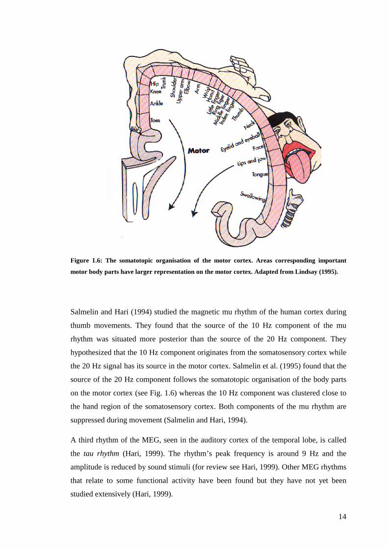
Figure 1.6: The somatotopic organisation of the motor cortex. Areas corresponding important
motor body parts have larger representation on the motor cortex. Adapted from Lindsay (1995).
Salmelin and Hari (1994) studied the magnetic mu rhythm of the human cortex during
thumb movements. They found that the source of the 10 Hz component of the mu
rhythm was situated more posterior than the source of the 20 Hz component. They
hypothesized that the 10 Hz component originates from the somatosensory cortex while
the 20 Hz signal has its source in the motor cortex. Salmelin et al. (1995) found that the
source of the 20 Hz component follows the somatotopic organisation of the body parts
on the motor cortex (see Fig. 1.6) whereas the 10 Hz component was clustered close to
the hand region of the somatosensory cortex. Both components of the mu rhythm are
suppressed during movement (Salmelin and Hari, 1994).
A third rhythm of the MEG, seen in the auditory cortex of the temporal lobe, is called
the tau rhythm (Hari, 1999). The rhythm’s peak frequency is around 9 Hz and the
amplitude is reduced by sound stimuli (for review see Hari, 1999). Other MEG rhythms
that relate to some functional activity have been found but they have not yet been
studied extensively (Hari, 1999).
15
The activation of the cortex during hand movements
The populations of neurons have been shown to either decrease or increase their
synchrony as a response to an event. This kind of phenomenon should be detected with
the help of frequency analysis. Motor behaviour and sensory stimulation can either
result in an amplitude suppression event-related desynchronization, (ERD) or in an
amplitude enhancement, event-related synchronisation (ERS) of the two components of
the mu rhythm (for review see, Pfurtscheller and Lopes da Silva, 1999). For more on
ERD/ERS, see section 1.4.2.
Several research groups (for reviews, see Pfurtscheller and Neuper, 2001 and Hari,
1999) have shown that during the preparation and execution of a motor act the
amplitudes of both the 10 Hz and of the 20 Hz react. Both studies reviewed
(Pfurtscheller et al., 1996 and Salenius et al., 1997) show that the enhancement of the
20 Hz component begins while the 10 Hz component is still suppressed.
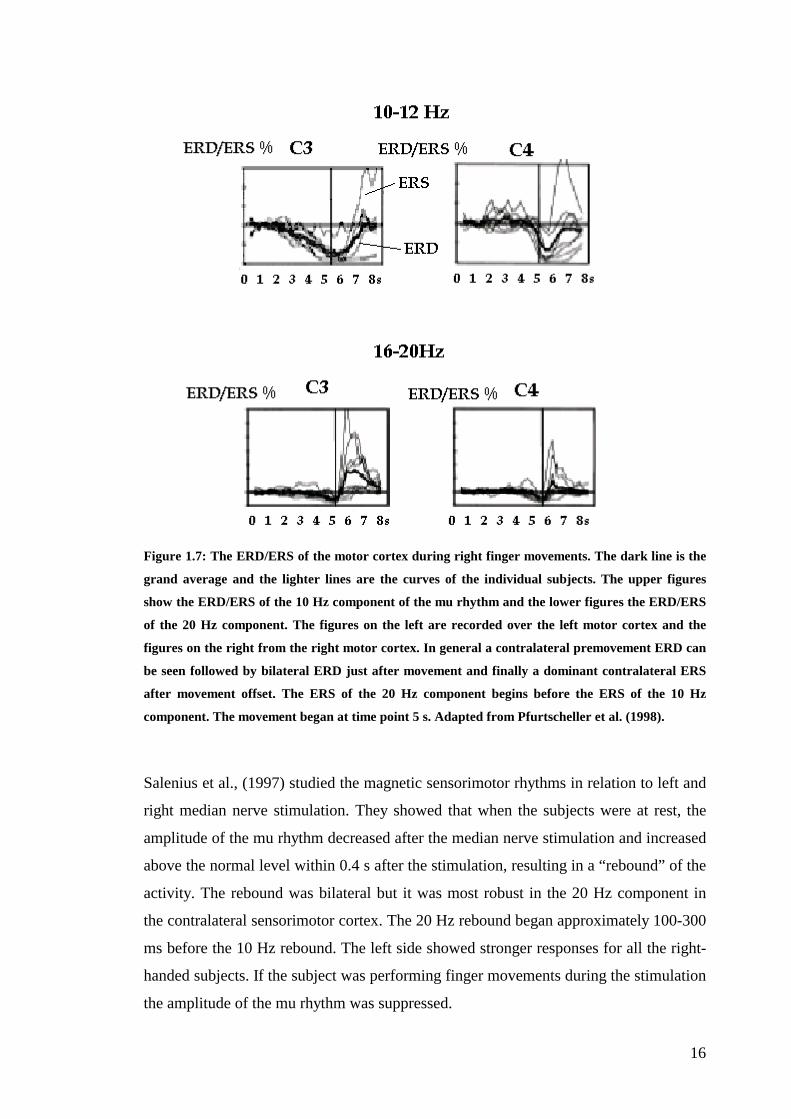
Pfurtscheller et al. (1996) studied the somatosensory rhythms of self-paced finger
extension. The ERD of the 10 Hz component began 2.5 s before movement onset. It
reached maximum shortly after movement onset and recovered to baseline level within
a couple of seconds. The ERD of the 20 Hz component on the other hand lasts only for
a short while, beginning just before the movement. The ERD of the 20 Hz component is
followed by an ERS that reaches its maximum just after the movement has ended. The
authors concluded that both the 10 Hz and 20 Hz component show first a contralateral
dominant desynchronization prior to movement and then a bilateral desynchronization
during movement, and finally a contralaterally dominant synchronisation of the 20 Hz
component (see Fig. 1.7).
16
Figure 1.7: The ERD/ERS of the motor cortex during right finger movements. The dark line is the
grand average and the lighter lines are the curves of the individual subjects. The upper figures
show the ERD/ERS of the 10 Hz component of the mu rhythm and the lower figures the ERD/ERS
of the 20 Hz component. The figures on the left are recorded over the left motor cortex and the
figures on the right from the right motor cortex. In general a contralateral premovement ERD can
be seen followed by bilateral ERD just after movement and finally a dominant contralateral ERS
after movement offset. The ERS of the 20 Hz component begins before the ERS of the 10 Hz
component. The movement began at time point 5 s. Adapted from Pfurtscheller et al. (1998).
Salenius et al., (1997) studied the magnetic sensorimotor rhythms in relation to left and
right median nerve stimulation. They showed that when the subjects were at rest, the
amplitude of the mu rhythm decreased after the median nerve stimulation and increased
above the normal level within 0.4 s after the stimulation, resulting in a “rebound” of the
activity. The rebound was bilateral but it was most robust in the 20 Hz component in
the contralateral sensorimotor cortex. The 20 Hz rebound began approximately 100-300
ms before the 10 Hz rebound. The left side showed stronger responses for all the right-
handed subjects. If the subject was performing finger movements during the stimulation
the amplitude of the mu rhythm was suppressed.
17
Different kinds of movement affect the rhythms of the cortex in different ways. Stancak
and Pfurtscheller (1996) showed that the post-movement 20 Hz component shows a
stronger rebound 0.25-0.75 s after brisk than after slow movement. It is also known that
when a person is performing a new task with his fingers, the contralateral
desynchronization of the 10 Hz component of the mu rhythm is enhanced. When the
movement is performed more automatically, the desynchronization is reduced (for
review see Pfurtscheller and Lopes da Silvia, 1999).
Salmelin and Hari (1994) concluded from a study including four subjects that self-
paced movements show a larger rebound of the mu rhythm than externally triggered
movement. The trigger used in this study was electrical stimulation of the median
nerve. Kaiser et al. (2000) acquired similar results when comparing a complex self-
paced finger movement and a simple externally paced finger movements. In a similar
study by Gerloff et al. (1998), an audible metronome was used as a trigger. Matching
results were obtained for the 20 Hz component of the mu rhythm. Three different self-
paced movements of the wrist, finger, and thumb, were studied by Pfurtscheller et al.
(1998). All three movements showed similar ERD patterns of the 10 Hz component
during preparation of the movements. The 20 Hz component in contrast showed
differences during the post-movement ERS. Wrist movements showed the largest
contralateral rebound. To sum up, it seems that the greatest activity could be detected
after a brisk, novel, self-paced wrist movement.
1.3.3 Motor imagery
Motor imagery can be defined as the conscious process of simulating movements
without their overt execution (Jeannerod, 1994). In a review article, Jeannerod (1994)
discusses several studies that have found that simulated actions take the same time as
executed ones. He concludes that motor imagery relies, at least in part, on the same
mechanisms as motor execution. It is widely accepted that mental imagination of
movements involves similar brain activation as when one is preparing such movements
(Crammond, 1997). It was first believed that the primary motor cortex is not involved
in mental imagery. More recent studies have, however, shown the involvement of the
primary motor cortex during imagination of movements (Schnitzler et al., 1997). EMG
activity, meaning the activity detected from the muscles, of the moving body part has
18
been reported in several studies concerning motor imagery. It is believed that the
detected EMG reflects some kind of activation of motor output and it can be detected
even during the imagination of movements (for review see Jeannerod, 1994).
In a MEG study, using median nerve stimulation, Schnitzler et al. (1997) investigated
the involvement of the primary motor cortex during motor imagery. The post stimulus
rebound of the 20 Hz rhythm was suppressed in a similar manner, but not to full extent,
as after execution of real movement. As with execution of movements, the effect was
predominantly observed on contralateral side of the motor cortex.
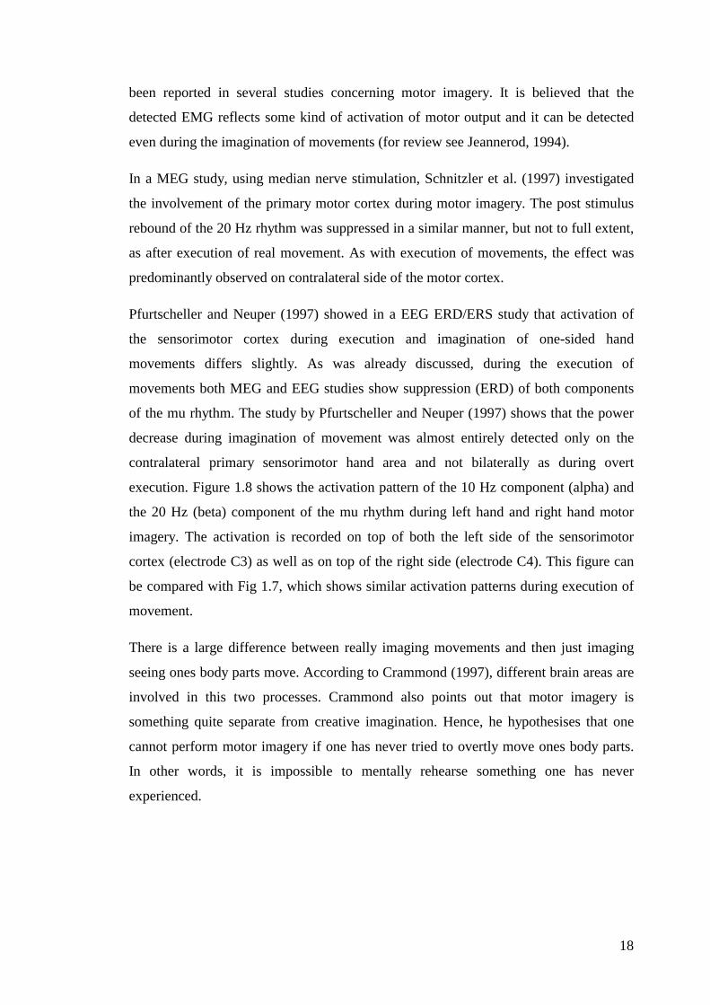
Pfurtscheller and Neuper (1997) showed in a EEG ERD/ERS study that activation of
the sensorimotor cortex during execution and imagination of one-sided hand
movements differs slightly. As was already discussed, during the execution of
movements both MEG and EEG studies show suppression (ERD) of both components
of the mu rhythm. The study by Pfurtscheller and Neuper (1997) shows that the power
decrease during imagination of movement was almost entirely detected only on the
contralateral primary sensorimotor hand area and not bilaterally as during overt
execution. Figure 1.8 shows the activation pattern of the 10 Hz component (alpha) and
the 20 Hz (beta) component of the mu rhythm during left hand and right hand motor
imagery. The activation is recorded on top of both the left side of the sensorimotor
cortex (electrode C3) as well as on top of the right side (electrode C4). This figure can
be compared with Fig 1.7, which shows similar activation patterns during execution of
movement.
There is a large difference between really imaging movements and then just imaging
seeing ones body parts move. According to Crammond (1997), different brain areas are
involved in this two processes. Crammond also points out that motor imagery is
something quite separate from creative imagination. Hence, he hypothesises that one
cannot perform motor imagery if one has never tried to overtly move ones body parts.
In other words, it is impossible to mentally rehearse something one has never
experienced.
19
Figure 1.8: Grand average ERD/ERS during motor imagery. Upper figures show the 10 Hz
component and the lower figures show the 20 Hs component of the activity. The figures on the left
are registered over the left sensorimotor cortex and the figures on the right over the right
sensorimotor cortex. The contralateral ERD can be seen during the imagination of the movement
and the contralateral ERS after the imagination. The grey bar illustrates the duration of the cue.
Pfurtscheller and Neuper (2001).
1.3.4 The activation of the sensorimotor cortex in paralysed
patients
The nature and extent of the adaptive changes that occur in the cerebral cortex
following an injury to e.g. the spinal cord are mostly unknown (Mikulis et al., 2002).
Nonetheless, the activation of the motor cortex of paralyzed patients is of great
importance when developing brain computer interfaces that are operated by activity
from the motor cortex.
Shoham et al. (2001), conducted an fMRI study on five spinal-cord damage patients.
The tetraplegics had been in an accident within five years of the study and were thus
not born paralysed. The activation of the sensorimotor cortex of the paralysed patients
when they attempted to execute a movement resembled of the activation of a healthy
20
person when he actually performed the movements. It is important to emphasise that
the patients were instructed to really try and move their body parts and to not imagine
doing so. Shoham et al. (2001) conclude from that the subjects’ motor cortex activation
closely follows the normal somatotopic organisation in the primary and non-primary
sensorimotor areas.
In a similar study by Sabbath et al. (2002), nine patients with complete spinal cord
injury were investigated by fMRI. The activation of the motor cortex was examined
when the patients where both attempting to execute movement of their toes and image
doing so. All patients showed activation of the sensorimotor cortices and only some
local cortical reorganisation was found.
21
1.4 Studying brain activation
1.4.1 Time domain analysis and event-related responses
MEG recordings consist of signals and noise. The neuromagnetic signals produced by
the neurons vary as a function of time. Signal processing is needed to separate the
information from the noise. MEG signals can be analysed in both time and frequency
domains.
External or internal stimuli give rise to characteristic patterns. In order to separate these
patterns from the background noise the MEG signal can be filtered and averaged, time-
locked to the stimuli. These signals are known as event-related fields (ERFs). Similar
signal processing can be applied to EEG signals and event-related potentials (ERPs) are
then obtained. ERFs/ERPs can be evaluated in both time and frequency domain but up
to now time domain analysis has been more common.
Several assumptions are made when ERFs/ERPs are calculated. First, one has to
assume that the signal itself, meaning the phase, form, frequency, latency, and
amplitude of the signal, is invariant across trials. In other words, one assumes that the
brain reacts in the same manner each time a stimulus is presented. Secondly, one has to
assume that the background noise of MEG/EEG is random and its mean is zero.
Stochastic properties of the noise are assumed to be invariant over time. Finally, the
information of the signal and the noise are believed to be uncorrelated (Elbert, 1998).
Typical ERP deflections are given names such as P300 or N100, in which P stands for
scalp-positive and N for vertex-negative. P300 is a positive peak in the potential on the
scalp that reaches a maximum of about 300 ms after the stimulus is presented on the
scalp, N100 on the other hand is a negative peak at the vertex at 100 ms. (Picton et al.,
2000). ERF values in contrast are given names such as M20, naming the magnetic
component only by their latency (see e.g. Kakigi et al., 2000) or N100m meaning the
magnetic counterpart of the electric N100. Of some interest for this Thesis are the
somatosensory evoked magnetic fields (SEFs) and the movement related magnetic
fields. The movement related magnetic fields have generally been divided into three
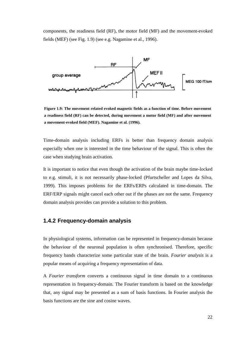
22
components, the readiness field (RF), the motor field (MF) and the movement-evoked
fields (MEF) (see Fig. 1.9) (see e.g. Nagamine et al., 1996).
Time-domain analysis including ERFs is better than frequency domain analysis
especially when one is interested in the time behaviour of the signal. This is often the
case when studying brain activation.
It is important to notice that even though the activation of the brain maybe time-locked
to e.g. stimuli, it is not necessarily phase-locked (Pfurtscheller and Lopes da Silva,
1999). This imposes problems for the ERFs/ERPs calculated in time-domain. The
ERF/ERP signals might cancel each other out if the phases are not the same. Frequency
domain analysis provides can provide a solution to this problem.
1.4.2 Frequency-domain analysis
In physiological systems, information can be represented in frequency-domain because
the behaviour of the neuronal population is often synchronised. Therefore, specific
frequency bands characterize some particular state of the brain. Fourier analysis is a
popular means of acquiring a frequency representation of data.
A Fourier transform converts a continuous signal in time domain to a continuous
representation in frequency-domain. The Fourier transform is based on the knowledge
that, any signal may be presented as a sum of basis functions. In Fourier analysis the
basis functions are the sine and cosine waves.
Figure 1.9: The movement related evoked magnetic fields as a function of time. Before movement
a readiness field (RF) can be detected, during movement a motor field (MF) and after movement
a movement-evoked field (MEF). Nagamine et al. (1996).
23
Biophysical signals like MEG are almost always digitised. Discrete Fourier transform
(DFT) has to be applied to such signals. The Discrete Fourier transform X(f) is given by
[ ]∑∞
−∞=
−=n
njj enxeX ωω)( (1.5)
where X(ejw) is the transform in frequency-domain and x[n] the sequence in time
domain. When sampling the continuous MEG signal into discrete parts one has to
remember to take into account Nyqvist’s sampling theorem. It states that a continuous
signal can be completely recovered from its samples if and only if the sampling rate is
greater than twice the highest frequency of the signal. In practical applications, the DFT
is usually computed with the fast Fourier transform (FFT). The formula of FFT
resembles equation (1.5). For more detailed information on Fourier analysis and digital
signal processing see Mitra (1998).
Fourier techniques assume stationarity of the signal. Stationarity is defined as a quality
of a process in which the statistical parameters, e.g. mean and standard deviation, of the
process do not change with time. Because MEG signals are far from stationary the
signal has to be divided into small segments of the order of 1 s. The frequency-domain
representation for each segment is calculated separately using short term Fourier
transform (STFT). STFT assumes that each segment is stationary. There is a time-
resolution trade-off when calculating the frequency representation of short segments.
The shorter the segment in time domain is, the better the time resolution. On the other
hand, a shorter segment in time domain gives a longer window in frequency-domain
resulting in a poorer frequency resolution.
In the following section two frequently used approaches will be reviewed.
Pfurtscheller and co-workers (for review see, Pfurtscheller and Lopes da Silva 1999)
study the relative increases and decreases of the power in certain frequency bands in
terms of event-related synchronisation and event-related desynchronization. When
calculating the ERS/ERD, Pfurtscheller usually refers the event-related activity in a
specific frequency band to a baseline level calculated in the same frequency band just
before the event happens. In this way the brain activation is normalised. Activation of
the neurons that is time-locked but not phase locked cannot be detected with the
24
conventional ERP technique. According to Pfurtscheller and Lopes da Silva, (1999) this
activation can be detected in the frequency-domain with the help ERD/ERS.
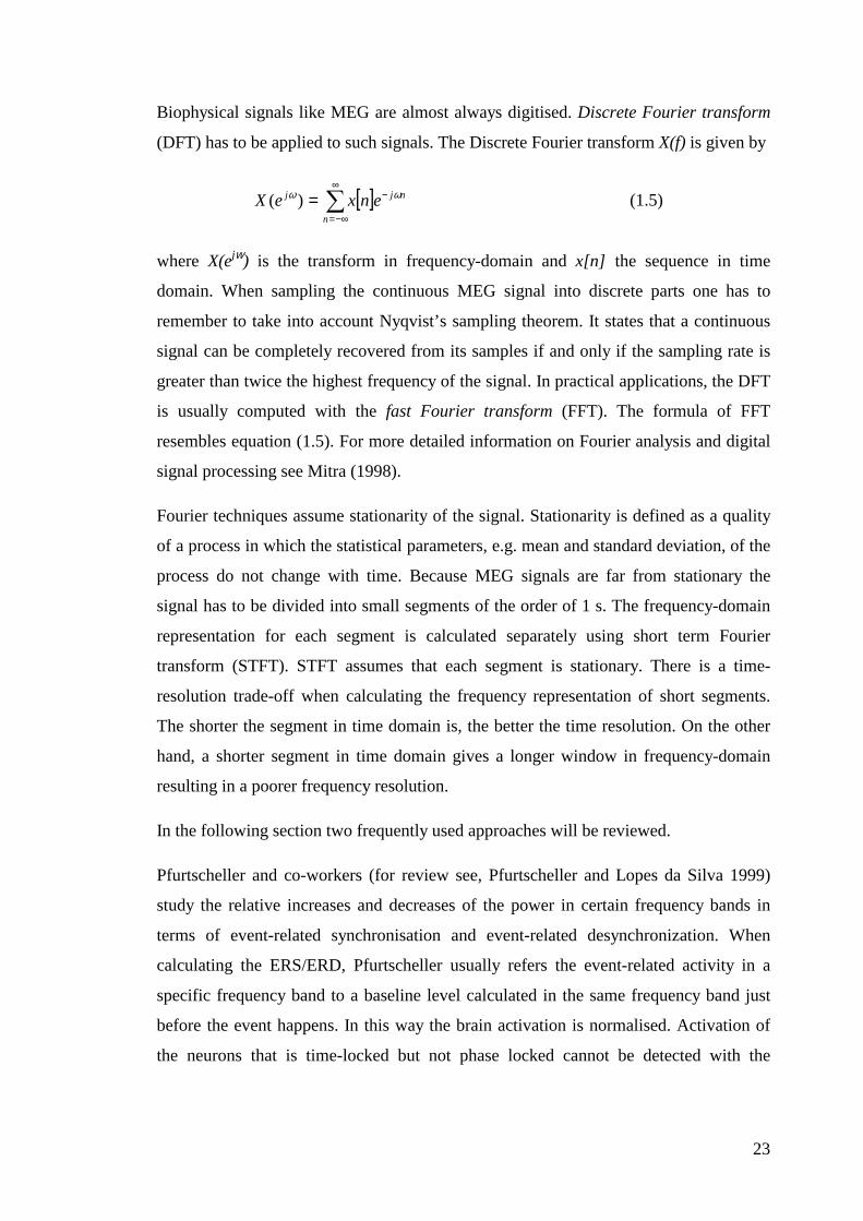
Salmelin and Hari (1994) use a temporal spectral evolution (TSE) analysis method to
analyze brain functioning in frequency-domain. TSE resembles the ERS/ERD method
except that TSE preserves the original units and does not refer the signal to some
baseline level. Figure 1.10 shows schematically the processing steps needed for the
TSE analysis. The brain signals are first bandpass filtered, then the absolute value of
the signal is calculated and finally the signals are averaged according to the triggers.
ORIGINAL SIGNAL
RECTIFIED
FILTERED 7-14 Hz
AVERAGED
TEMPORAL SPECTRAL EVOLUTION
ORIGINAL SIGNAL
RECTIFIED
FILTERED 7-14 Hz
AVERAGED
TEMPORAL SPECTRAL EVOLUTION
ORIGINAL SIGNAL
RECTIFIED
FILTERED 7-14 Hz
AVERAGED
ORIGINAL SIGNAL
RECTIFIED
FILTERED 7-14 Hz
AVERAGED
TEMPORAL SPECTRAL EVOLUTION
1.4.3 Time-frequency representation and wavelets
Frequency analysis is one of the means to study brain activation. Nonetheless, a
frequency representation does not tell us where in the transformed segment of the
Figure 1.10: The different steps of the TSE analysis. First the original signal is filtered, then
rectified and finally averaged. Modified from Hari and Salmelin (1994).
25
signal, certain frequencies are present. The solution to this problem is to look at time-
frequency representations. TFR is a means to present the power of a continuous signal
as a function of both time and frequency.
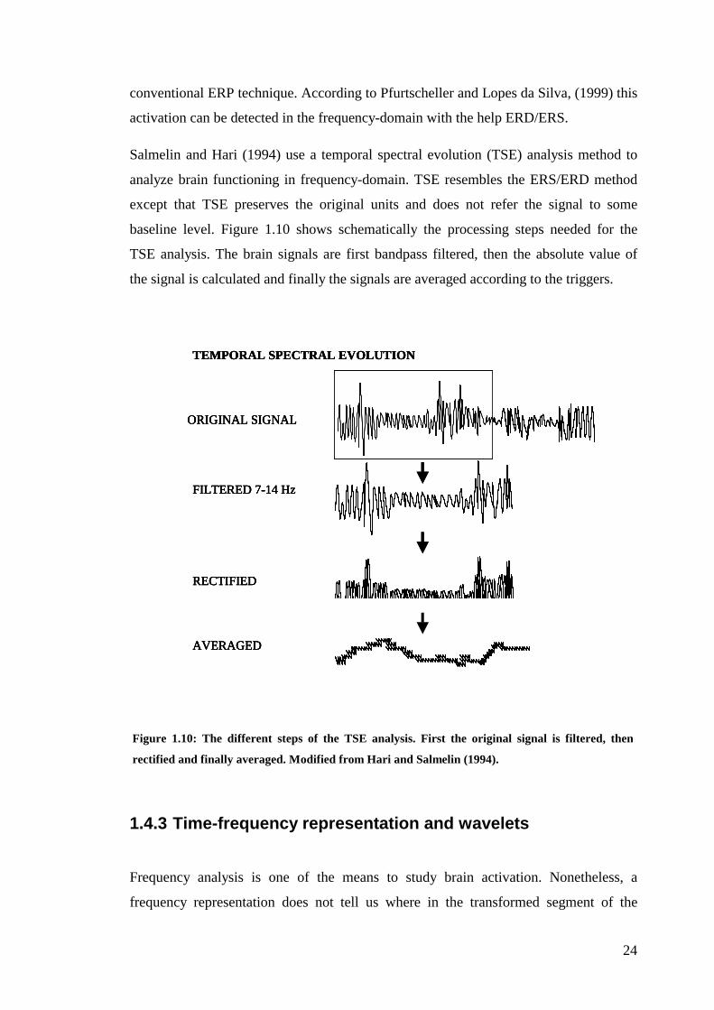
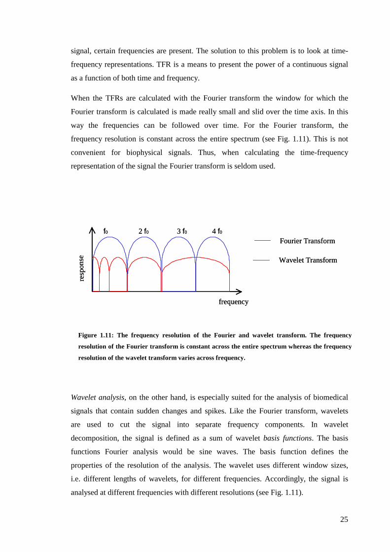
When the TFRs are calculated with the Fourier transform the window for which the
Fourier transform is calculated is made really small and slid over the time axis. In this
way the frequencies can be followed over time. For the Fourier transform, the
frequency resolution is constant across the entire spectrum (see Fig. 1.11). This is not
convenient for biophysical signals. Thus, when calculating the time-frequency
representation of the signal the Fourier transform is seldom used.
Wavelet analysis, on the other hand, is especially suited for the analysis of biomedical
signals that contain sudden changes and spikes. Like the Fourier transform, wavelets
are used to cut the signal into separate frequency components. In wavelet
decomposition, the signal is defined as a sum of wavelet basis functions. The basis
functions Fourier analysis would be sine waves. The basis function defines the
properties of the resolution of the analysis. The wavelet uses different window sizes,
i.e. different lengths of wavelets, for different frequencies. Accordingly, the signal is
analysed at different frequencies with different resolutions (see Fig. 1.11).
frequency
4 f02 f0f0 3 f0
resp
onse
Fourier Transform
Wavelet Transform
frequency
4 f02 f0f0 3 f0
resp
onse
Fourier Transform
Wavelet Transform
Figure 1.11: The frequency resolution of the Fourier and wavelet transform. The frequency
resolution of the Fourier transform is constant across the entire spectrum whereas the frequency
resolution of the wavelet transform varies across frequency.
26
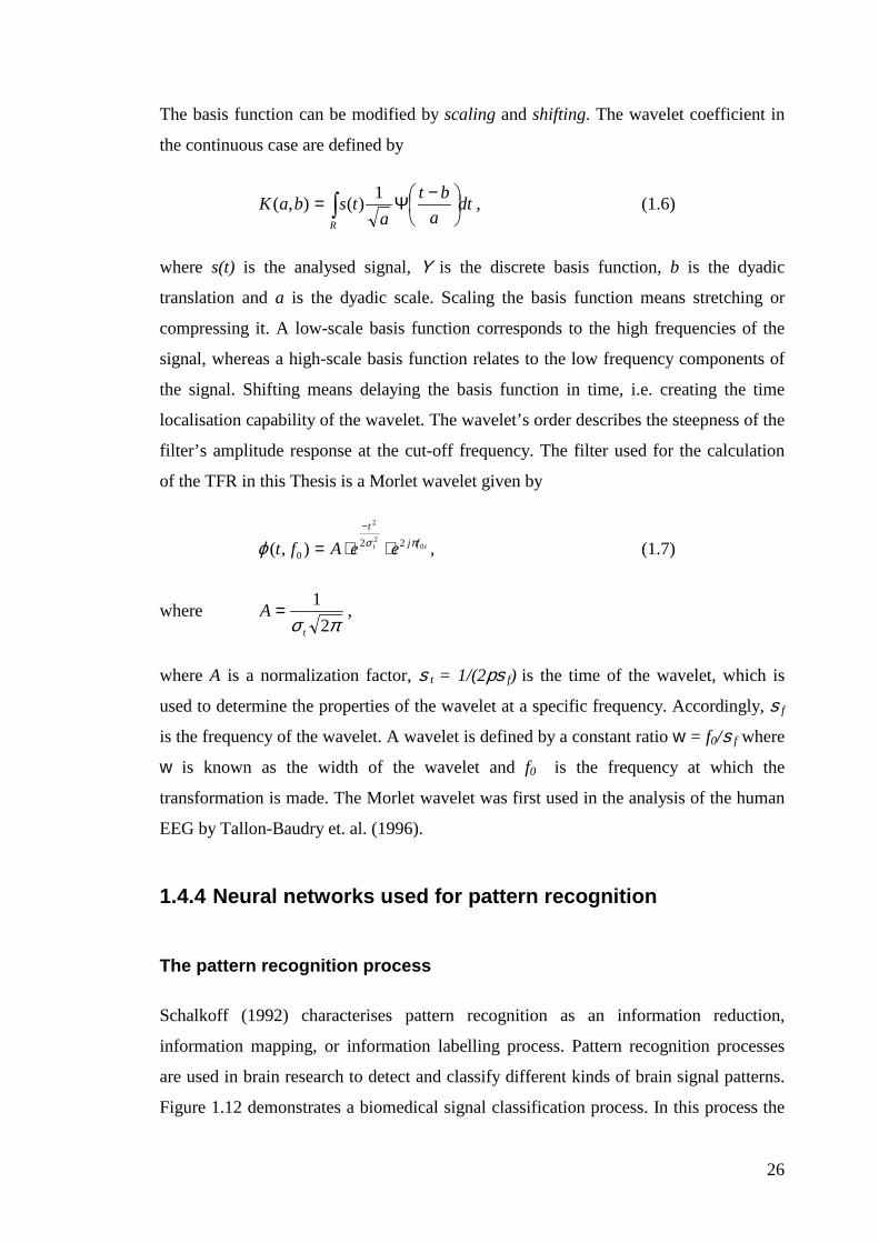
The basis function can be modified by scaling and shifting. The wavelet coefficient in
the continuous case are defined by
dta
bt
atsbaK
R∫
−Ψ= 1
)(),( , (1.6)
where s(t) is the analysed signal, Y is the discrete basis function, b is the dyadic
translation and a is the dyadic scale. Scaling the basis function means stretching or
compressing it. A low-scale basis function corresponds to the high frequencies of the
signal, whereas a high-scale basis function relates to the low frequency components of
the signal. Shifting means delaying the basis function in time, i.e. creating the time
localisation capability of the wavelet. The wavelet’s order describes the steepness of the
filter’s amplitude response at the cut-off frequency. The filter used for the calculation
of the TFR in this Thesis is a Morlet wavelet given by
,),( 02
2
220
tt fj
t
eeAft πσϕ ⋅⋅=−
(1.7)
where πσ 2
1
t
A = ,
where A is a normalization factor, st = 1/(2psf) is the time of the wavelet, which is
used to determine the properties of the wavelet at a specific frequency. Accordingly, sf
is the frequency of the wavelet. A wavelet is defined by a constant ratio w = f0/sf where
w is known as the width of the wavelet and f0 is the frequency at which the
transformation is made. The Morlet wavelet was first used in the analysis of the human
EEG by Tallon-Baudry et. al. (1996).
1.4.4 Neural networks used for pattern recognition
The pattern recognition process
Schalkoff (1992) characterises pattern recognition as an information reduction,
information mapping, or information labelling process. Pattern recognition processes
are used in brain research to detect and classify different kinds of brain signal patterns.
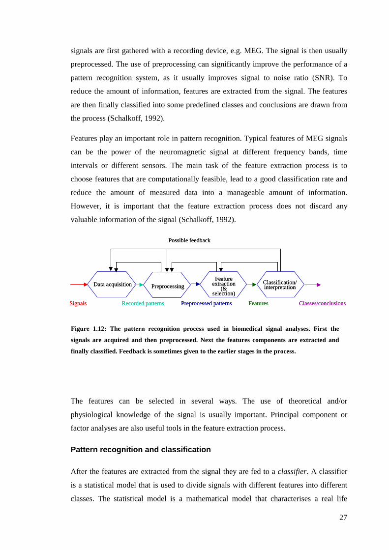
Figure 1.12 demonstrates a biomedical signal classification process. In this process the
27
signals are first gathered with a recording device, e.g. MEG. The signal is then usually
preprocessed. The use of preprocessing can significantly improve the performance of a
pattern recognition system, as it usually improves signal to noise ratio (SNR). To
reduce the amount of information, features are extracted from the signal. The features
are then finally classified into some predefined classes and conclusions are drawn from
the process (Schalkoff, 1992).
Features play an important role in pattern recognition. Typical features of MEG signals
can be the power of the neuromagnetic signal at different frequency bands, time
intervals or different sensors. The main task of the feature extraction process is to
choose features that are computationally feasible, lead to a good classification rate and
reduce the amount of measured data into a manageable amount of information.
However, it is important that the feature extraction process does not discard any
valuable information of the signal (Schalkoff, 1992).
Feature extraction
(& selection)
Classification/ interpretation
Signals Classes/conclusionsPreprocessed patternsRecorded patterns Features
Possible feedback
Data acquisition PreprocessingFeature
extraction (&
selection)
Classification/ interpretation
Signals Classes/conclusionsPreprocessed patternsRecorded patterns Features
Possible feedback
Data acquisition Preprocessing
The features can be selected in several ways. The use of theoretical and/or
physiological knowledge of the signal is usually important. Principal component or
factor analyses are also useful tools in the feature extraction process.
Pattern recognition and classification
After the features are extracted from the signal they are fed to a classifier. A classifier
is a statistical model that is used to divide signals with different features into different
classes. The statistical model is a mathematical model that characterises a real life
Figure 1.12: The pattern recognition process used in biomedical signal analyses. First the
signals are acquired and then preprocessed. Next the features components are extracted and
finally classified. Feedback is sometimes given to the earlier stages in the process.
28
phenomenon, such as a MEG response to a specific stimulus, with help of mathematical
methods. In this Thesis these statistical mathematical models are used to classify
different sorts of brain activity into different classes.
The observed signals about the examined phenomenon consist of both information and
noise. Information in this case means the activation of the brain triggered by an event.
The model has to be able to describe the characteristics of the phenomenon as well as
possible. However, it cannot be too specific because then it would model the noise in
addition to the information, which is not preferable. Even though the model is built
upon some examples of the phenomenon it should generalise to represent the whole
phenomena.
Classification is principally performed by determining a decision region in feature
space. Each decision region corresponds to a classification class. The shape of the
decision boundary depends on the characteristics of the classifier. An example of a two-
dimensional feature space with a decision boundary can be seen in Fig. 1.13 (Bishop,
1995).
Several artificial neural network (ANN) based classifiers are used in classifying
biomedical signals. An ANN refers to an information processing structure that
resembles the neural system present in the brain. Biological networks have actually
inspired many concepts in neural computing. Basically an ANN is a mathematical
function.
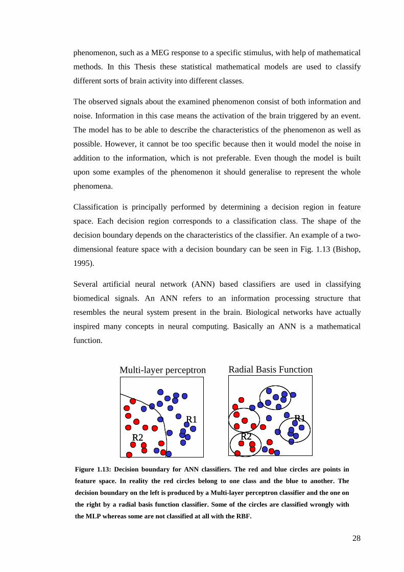
Figure 1.13: Decision boundary for ANN classifiers. The red and blue circles are points in
feature space. In reality the red circles belong to one class and the blue to another. The
decision boundary on the left is produced by a Multi-layer perceptron classifier and the one on
the right by a radial basis function classifier. Some of the circles are classified wrongly with
the MLP whereas some are not classified at all with the RBF.
R1
R2
R1
R2
R1
R2
R1
R2
R1
R2
Multi-layer perceptron Radial Basis Function
29
A decision boundary for ANN classifiers. The red and blue circles are the points in the
feature space. In reality the red circles belong to one class and the blue circles to
another. The feature space can be divided into classes linearly and nonlinearly. The
decision boundary on the left is linear. The picture on the right is for a non-linear
decision boundary. Some of the circles are classified wrongly with the linear classifier.
These pictures only illustrate a two dimensional input space, meaning that only two
different features are used
Nykopp (2001) compared two different ANN based classifiers for the classification of
EEG signals for the use of a brain computer interface. The studied classifiers where the
linear classifier Radial Basis Function (RBF) –net and the non-linear model Multi
Layer Perceptron (MLP). These neural networks are discussed in detail in the following
sections. This Thesis will use these two classifiers when classifying the magnetic brain
signals.
Multi-layer perceptron
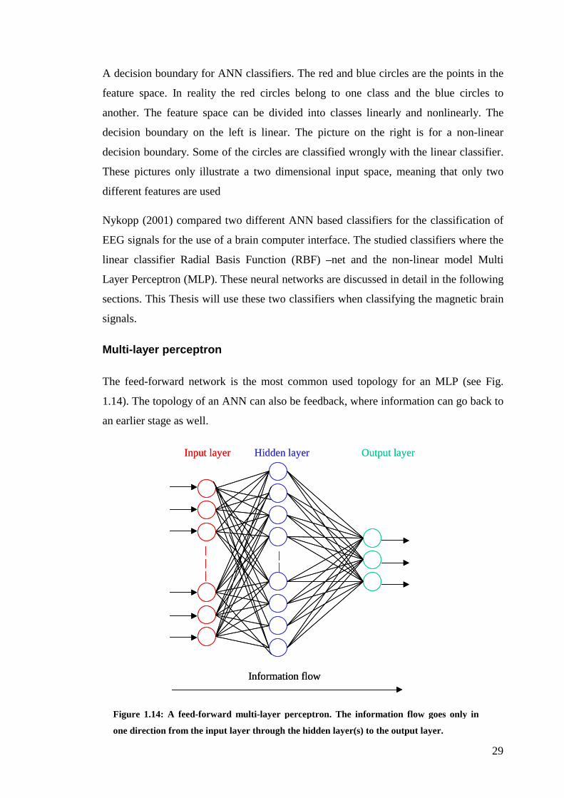
The feed-forward network is the most common used topology for an MLP (see Fig.
1.14). The topology of an ANN can also be feedback, where information can go back to
an earlier stage as well.
Hidden layerInput layer Output layer
Information flow
Hidden layerInput layer Output layer
Information flow
Figure 1.14: A feed-forward multi-layer perceptron. The information flow goes only in
one direction from the input layer through the hidden layer(s) to the output layer.
30
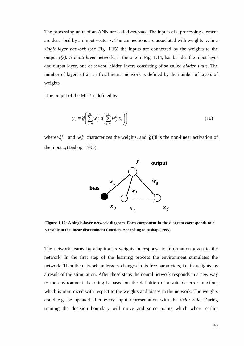
The processing units of an ANN are called neurons. The inputs of a processing element
are described by an input vector x. The connections are associated with weights w. In a
single-layer network (see Fig. 1.15) the inputs are connected by the weights to the
output y(x). A multi-layer network, as the one in Fig. 1.14, has besides the input layer
and output layer, one or several hidden layers consisting of so called hidden units. The
number of layers of an artificial neural network is defined by the number of layers of
weights.
The output of the MLP is defined by
( )
= ∑ ∑= =
M
j
d
iijikjk xwgwgy
0 0
)1(2~ (10)
where )2(kjw and )1(
jiw characterizes the weights, and )(~ ⋅g is the non-linear activation of
the input xi (Bishop, 1995).
The network learns by adapting its weights in response to information given to the
network. In the first step of the learning process the environment stimulates the
network. Then the network undergoes changes in its free parameters, i.e. its weights, as
a result of the stimulation. After these steps the neural network responds in a new way
to the environment. Learning is based on the definition of a suitable error function,
which is minimized with respect to the weights and biases in the network. The weights
could e.g. be updated after every input representation with the delta rule. During
training the decision boundary will move and some points which where earlier
y
w1
w0
x dx 0 x 1
wdbias
output
inputs
y
w1w1
w0w0
x dx dx 0x 0 x 1x 1
wdwdbias
output
inputsFigure 1.15: A single-layer network diagram. Each component in the diagram corresponds to a
variable in the linear discriminant function. According to Bishop (1995).

31
misclassified will become correctly classified. This kind of learning is called supervised
learning because the data has been prelabelled and the expected output of an input is
known. An ANN can also be taught using unsupervised learning when there is no
desired output (Bishop, 1995).
Radial basis function networks
As the MLP network the RBF is also a statistical model used to classify signals into
classes. The architecture of the RBF is very similar to that of the MLP in Fig. 1.14. The
major difference is that the output of the RBF network is a radial basis function.
Several different basis functions can be used in the discriminant function of the RBF.
The Gaussian basis function is commonly used and it is given by
−=
2
22exp)(
j
j
j
xx
σµ
φ (11)
where x is the input vector of the RBF, m is the vector that determines the centre of the
basis function and sj is the width vector that controls the smoothness of the function.
The activation of a hidden unit in the RBF is determined by the distance between the
input vector and a prototype vector (Bishop, 1995).
The most general RBF is composed of two layers of weights with different roles. The
RBF is trained in two stages. In the first stage the input data set is used to determine the
parameters of the basis functions. This learning process is unsupervised. The basis
function is characterised by the first layer of weights. During the second stage the basis
function’s parameters are kept constant, as the second layer of weights are trained. This
training is supervised because the error function of the output and the excepted output
is utilised in the training process (Bishop, 1995).
Evaluation of pattern recognition techniques
How does one know if the classifier one has chosen is high quality or not? The results
of one pattern recognition approach can be compared with another approach in several
ways. First, the error rate of the classifier can be inspected. An error in this case means
a misclassification, an input that has been classified wrongly. The error rate is given by
32
Error rate = number of errors/ number of cases (12)
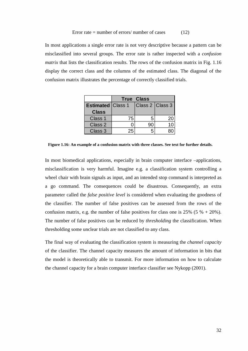
In most applications a single error rate is not very descriptive because a pattern can be
misclassified into several groups. The error rate is rather inspected with a confusion
matrix that lists the classification results. The rows of the confusion matrix in Fig. 1.16
display the correct class and the columns of the estimated class. The diagonal of the
confusion matrix illustrates the percentage of correctly classified trials.
In most biomedical applications, especially in brain computer interface –applications,
misclassification is very harmful. Imagine e.g. a classification system controlling a
wheel chair with brain signals as input, and an intended stop command is interpreted as
a go command. The consequences could be disastrous. Consequently, an extra
parameter called the false positive level is considered when evaluating the goodness of
the classifier. The number of false positives can be assessed from the rows of the
confusion matrix, e.g. the number of false positives for class one is 25% (5 % + 20%).
The number of false positives can be reduced by thresholding the classification. When
thresholding some unclear trials are not classified to any class.
The final way of evaluating the classification system is measuring the channel capacity
of the classifier. The channel capacity measures the amount of information in bits that
the model is theoretically able to transmit. For more information on how to calculate
the channel capacity for a brain computer interface classifier see Nykopp (2001).
True Class Estimated Class 1 Class 2 Class 3
ClassClass 1 75 5 20Class 2 0 90 10Class 3 25 5 80
Figure 1.16: An example of a confusion matrix with three classes. See text for further details.
33
1.5 Brain computer interfaces
1.5.1 Definition of a brain computer interface
A Brain Computer Interface is a device, which enables people to interact with
computer-based system through conscious control of their thoughts. There are two main
types of applications. In the first type the device uses artificially generated electrical
signals to stimulate brain tissue. This could, e.g., be an artificial retina. The second type
of device uses real-time sampling and processing of brain activity to control a
computer-based device. This Thesis will exclusively concentrate on the second type.
A BCI is capable of extracting some meaningful information from the brain with the
help of, e.g., artificial neural networks. A variety of brain imaging methods, such as
EEG, MEG, functional magnetic resonance imaging (fMRI), positron emission
tomography (PET) and invasive techniques such as microelectrodes placed in the brain,
could be used in BCIs. Most BCIs up to date are non-invasive and built upon the
analysis of EEG signals. The other techniques are regarded as technically demanding
and expensive (for recent review, see Wolpaw et al, 2002).
The idea of using brain signals for communication and controlling appliances sounds
very appealing. Brain mechanisms involved in motor control has been extensively
studied. Consequently, one might think that classifying brain signals into categories
would be trivial. But why is it not as easy to use these brain signals in brain computer
interfaces as it is when practising basic research? In most brain studies, the brain
signals related to an event are averaged over tens or hundreds of trials before the
activation can be distinguished from the brain’s background activity. Averaging
enhances the SNR. In addition, heavy computing has to be performed offline before any
results can be achieved. One of the major challenges when developing a BCI is to
detect the activation related to, e.g., motor intention from the brain’s background
activation, based on only one to a few trials. In addition, the classification should
happen online, preferable milliseconds after the event has occurred.
34
1.5.2 Brain interfaces based on electroencephalography
Vaughan et al. (1996) proposed two major BCI categories. These using EEG
deflections evoked by specific sensory stimulus and those using information in
spontaneous EEG. Wolpaw et al. (2002) called these “dependent” and “independent”
BCIs. The dependent BCI uses the brains normal output pathways whereas the
independent does not.
Donchin et al. (2000) developed a dependent BCI where rows and columns of letters
are flashed to the user and the visual evoked potentials (VEPs) are recorded. The BCI is
based on the knowledge that the P300 deflection is the largest to a letter the user wants
to choose. By picking the row and column that showed the largest P300 deflection the
BCI can determine what letter the user was interested in. This BCI is dependent on the
brain’s visual pathway.
The independent method is based on the recognition of mental states. The independent
method can further be divided into two sub categories. The first is known as the pattern
recognition approach. In this method the BCI tries to categorize different kinds of brain
signals caused by different mental activity into different classes. The pattern
recognition approach is used among others by Pfurtscheller and co-authors (see e.g.
Pfurtscheller et al. 2000). The second approach is known as the operant conditioning
approach, in which the user of the BCI tries to control his or her own brain rhythms.
This approach is used the by Wolpaw et al. (2000) and Birmbaumer et al. (2000). For a
recent review on the work of the different BCI groups, see the Master’s Thesis by
Lehtonen (2002).
The adaptive brain computer interface (ABI)
A recent ABI project (see e.g. Millan et al., 1998) sought to build an individual brain
interface, which is based on a mutual learning process where both the user and the ABI
adapt to each other. The interface adapts to its client as the artificial neural network
learns user-specific EEG patterns on the basis of which it classifies different mental
tasks. The user performs some predefined mental tasks such as imaging left or right
hand movement. The user is given feedback during the training session so that he can
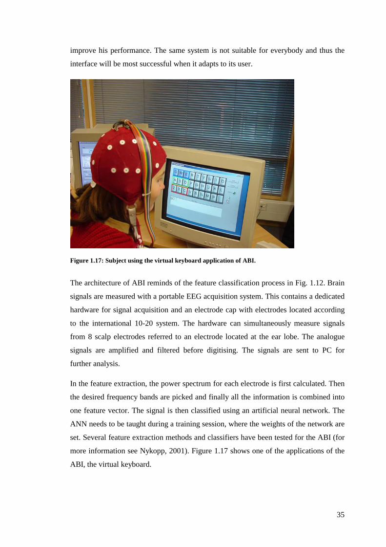
35
improve his performance. The same system is not suitable for everybody and thus the
interface will be most successful when it adapts to its user.
Figure 1.17: Subject using the virtual keyboard application of ABI.
The architecture of ABI reminds of the feature classification process in Fig. 1.12. Brain
signals are measured with a portable EEG acquisition system. This contains a dedicated
hardware for signal acquisition and an electrode cap with electrodes located according
to the international 10-20 system. The hardware can simultaneously measure signals
from 8 scalp electrodes referred to an electrode located at the ear lobe. The analogue
signals are amplified and filtered before digitising. The signals are sent to PC for
further analysis.
In the feature extraction, the power spectrum for each electrode is first calculated. Then
the desired frequency bands are picked and finally all the information is combined into
one feature vector. The signal is then classified using an artificial neural network. The
ANN needs to be taught during a training session, where the weights of the network are
set. Several feature extraction methods and classifiers have been tested for the ABI (for
more information see Nykopp, 2001). Figure 1.17 shows one of the applications of the
ABI, the virtual keyboard.

36
1.5.3 Brain computer interfaces used with other recording
techniques
EEG-based BCIs can be made portable, which is beneficial for applications. However,
electrical brain signals picked up by EEG are distorted by the skull and are thus not
very well localised. MEG signals on the other hand are not affected by the skull and are
consequently much more localised than EEG signals. Even so, not a single study could
be found where single trial MEG signals are classified online for BCI use.
Parra et al. (2001) classified both multi channel MEG and EEG single trials, offline. In
their MEG experiment, the subjects’ had to press a button in response to a light flash.
The subjects used either the right finger or left finger, related to the side of the light.
The subjects received auditory feedback after they had pressed the button. The trials
where classified, based on signals integrated from spatially distributed sensors. The
activations for the signals were selected before the movement began. Parra et al. (2001)
conclude that single-trial discrimination of a motor task from MEG signals is possible
using linear analyses methods.
Portin et al., (1996) classified MEG single trial signals of real movement using a self-
organizing map. Five subjects were instructed to perform brisk opposition movements
alternately with the left and right thumb once every 8 s. Altogether 40-80 movements
were performed. The feature vectors consisted of spectral components from single trials
obtained from 28-32 sensors above the sensorimotor cortex. Premovement,
postmovement as well as the activation patterns during movements were inspected
separately. The classification results for all movement stages showed large variability.
The classification rate was seldom better than random classification. In the study, 85 %
of the trials were classified correctly when an individual time period for each subject
was picked around the time of the movements. The classifier was unable to
discriminate on which side the movement was performed.
In 2000, Wessberg et al. were able to translate neuronal activity straightly from the
brain into robot commands. Microwires, recording the activation of only 50-100
neurons, were implanted in the monkey motor cortex. The monkey was, after the
training of the algorithms, able to control a robot arm by moving a joystick. The
computer predicted the movement 50-100 ms before it even happened and the robot
37
arm could be seen to move in the same way as the monkey arm. A year later Nicolelis
and co-workers (for recent review, see Nicolelis and Chapin, 2002) taught another
monkey to control a robot arm just by imaging moving a lever arm. The effect of visual
feedback was crucial while teaching the monkey.
Taylor et al. (2002) also emphasized the role of feedback. In their study, monkeys made
real and imaged arm movements in a computer generated three-dimensional virtual
environment. The activation of the motor cortex was recorded from approximately 20
neurons. The monkeys were first taught to move a cursor to a target on a computer
screen by moving their hands. The computer that controlled the cursor responded to the
activation of the motor cortex. During the whole training session the monkeys did not
actually see the movement of their hands, the only feedback was the cursor moving on
the screen. With time the monkeys learned to move the cursor without even moving
their arms. In other words, the neurons of the monkey had specialized in moving the
cursor. This study shows that brain easily adapts to the situation. These results are of
importance when building brain-controlled devices.

38
2 Method
2.1 Subjects and procedure
Data originally collected by Auranen (2002) were used. Five healthy, right-handed,
subjects (S1-S5) were randomly chosen out of 11. Three subjects were males. All
subjects were native speakers of Finnish. The age range was 22 - 25 years.
2.1.1 Experimental procedure
During the experiment the subjects were shown visual stimuli. Depending on the
stimuli, the subjects were asked to react by either slowly lifting their right or left index
finger 2-3 cm or then by imaging doing so. The experiment also consisted of neutral
trials where the subjects were instructed to do nothing. Fig. 2.1 demonstrates the
experimental set-up of a right lift trial. The experimental set-up of all the other trials
was analogous, except that the cue varied.
In each trial the subjects saw first a green square for 1 s, and then a cue that informed
what movement they were to perform. After the cue vanished, a red square appeared for
500 ms. The subjects where instructed to perform the task, indicated by the cue,
immediately after the red square disappeared. The subjects had 5 s to perform the task
before a green square reappeared. The experiment consisted of 40 trials of each tasks.
The order of the trials was randomly varied. The background of the screen was black.
The subjects were instructed to avoid blinks during the imagined or real finger
movements and blink if necessary during the green squares.
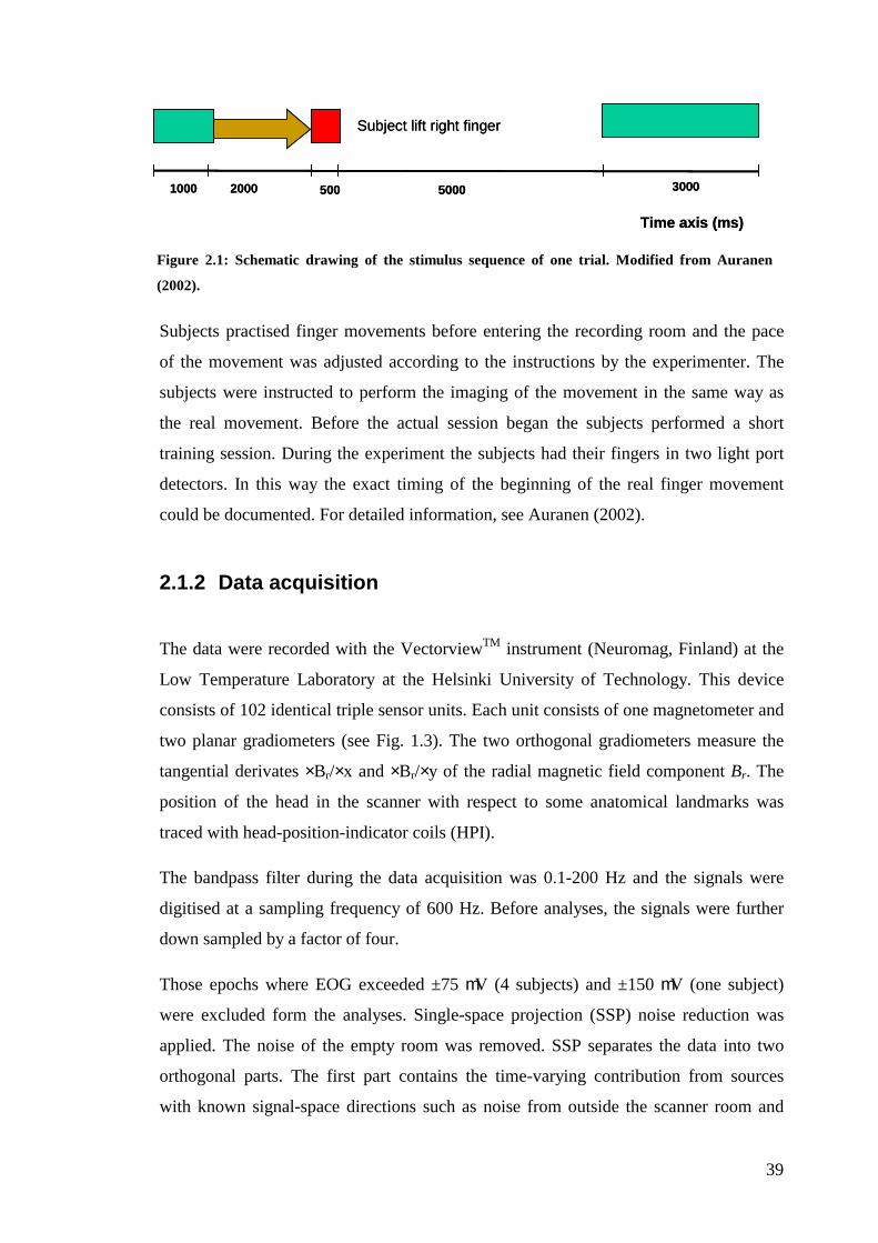
39
Subjects practised finger movements before entering the recording room and the pace
of the movement was adjusted according to the instructions by the experimenter. The
subjects were instructed to perform the imaging of the movement in the same way as
the real movement. Before the actual session began the subjects performed a short
training session. During the experiment the subjects had their fingers in two light port
detectors. In this way the exact timing of the beginning of the real finger movement
could be documented. For detailed information, see Auranen (2002).
2.1.2 Data acquisition
The data were recorded with the VectorviewTM instrument (Neuromag, Finland) at the
Low Temperature Laboratory at the Helsinki University of Technology. This device
consists of 102 identical triple sensor units. Each unit consists of one magnetometer and
two planar gradiometers (see Fig. 1.3). The two orthogonal gradiometers measure the
tangential derivates ∑Br/∑x and ∑Br/∑y of the radial magnetic field component Br. The
position of the head in the scanner with respect to some anatomical landmarks was
traced with head-position-indicator coils (HPI).
The bandpass filter during the data acquisition was 0.1-200 Hz and the signals were
digitised at a sampling frequency of 600 Hz. Before analyses, the signals were further
down sampled by a factor of four.
Those epochs where EOG exceeded ±75 mV (4 subjects) and ±150 mV (one subject)
were excluded form the analyses. Single-space projection (SSP) noise reduction was
applied. The noise of the empty room was removed. SSP separates the data into two
orthogonal parts. The first part contains the time-varying contribution from sources
with known signal-space directions such as noise from outside the scanner room and
3000500050020001000
Time axis (ms)
Subject lift right finger
3000500050020001000
Time axis (ms)
Subject lift right finger
Figure 2.1: Schematic drawing of the stimulus sequence of one trial. Modified from Auranen
(2002).
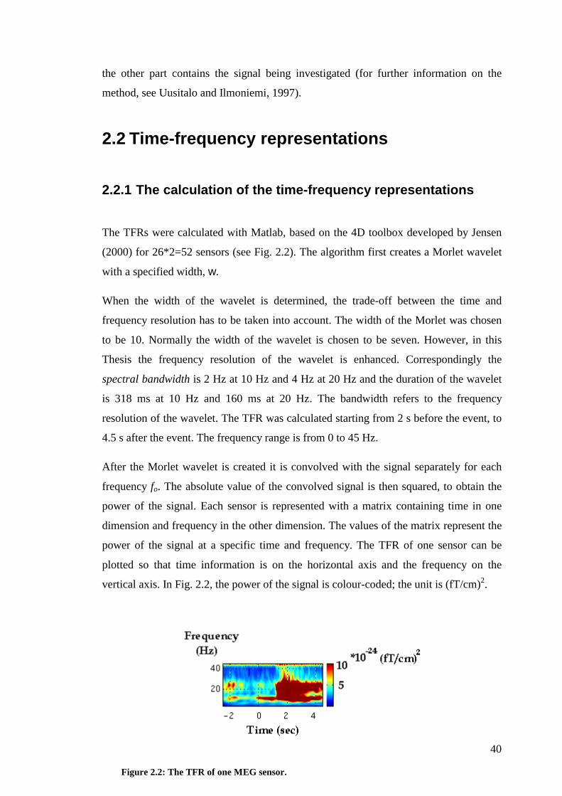
40
Figure 2.2: The TFR of one MEG sensor.
the other part contains the signal being investigated (for further information on the
method, see Uusitalo and Ilmoniemi, 1997).
2.2 Time-frequency representations
2.2.1 The calculation of the time-frequency representations
The TFRs were calculated with Matlab, based on the 4D toolbox developed by Jensen
(2000) for 26*2=52 sensors (see Fig. 2.2). The algorithm first creates a Morlet wavelet
with a specified width, w.
When the width of the wavelet is determined, the trade-off between the time and
frequency resolution has to be taken into account. The width of the Morlet was chosen
to be 10. Normally the width of the wavelet is chosen to be seven. However, in this
Thesis the frequency resolution of the wavelet is enhanced. Correspondingly the
spectral bandwidth is 2 Hz at 10 Hz and 4 Hz at 20 Hz and the duration of the wavelet
is 318 ms at 10 Hz and 160 ms at 20 Hz. The bandwidth refers to the frequency
resolution of the wavelet. The TFR was calculated starting from 2 s before the event, to
4.5 s after the event. The frequency range is from 0 to 45 Hz.
After the Morlet wavelet is created it is convolved with the signal separately for each
frequency fo. The absolute value of the convolved signal is then squared, to obtain the
power of the signal. Each sensor is represented with a matrix containing time in one
dimension and frequency in the other dimension. The values of the matrix represent the
power of the signal at a specific time and frequency. The TFR of one sensor can be
plotted so that time information is on the horizontal axis and the frequency on the
vertical axis. In Fig. 2.2, the power of the signal is colour-coded; the unit is (fT/cm)2.
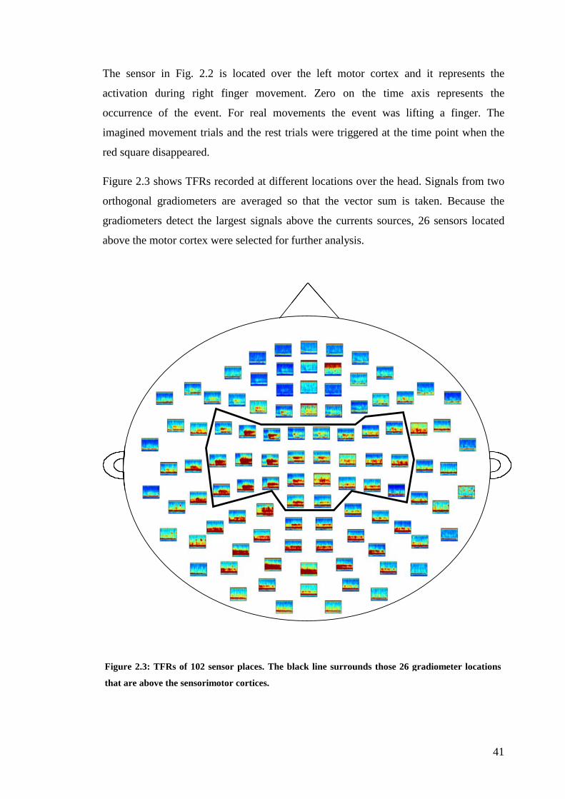
41
The sensor in Fig. 2.2 is located over the left motor cortex and it represents the
activation during right finger movement. Zero on the time axis represents the
occurrence of the event. For real movements the event was lifting a finger. The
imagined movement trials and the rest trials were triggered at the time point when the
red square disappeared.
Figure 2.3 shows TFRs recorded at different locations over the head. Signals from two
orthogonal gradiometers are averaged so that the vector sum is taken. Because the
gradiometers detect the largest signals above the currents sources, 26 sensors located
above the motor cortex were selected for further analysis.
Figure 2.3: TFRs of 102 sensor places. The black line surrounds those 26 gradiometer locations
that are above the sensorimotor cortices.
42
The calculated time-frequency representations
The TFRs were calculated in three ways: 1) single trials of each subject, 2) trials
averaged for each subject, 3) trials averaged over all subjects (grand averages). The
TFRs were calculated for each task. In addition, two to four consecutive single trial
TFRs were averaged, to study the effect of the improvement of SNR. To this aim, the
four first trials of each task were used.
For each subject, typically 30-40 trials were averaged. The subject averages as well as
the grand averages were used to define features used in signal classification.
2.3 Pattern recognition and classification
The classification process involves three steps: preprocessing, feature extraction and
feature classification. The details of this process are discussed in section 1.4.4 and the
process itself is summarised in Fig. 1.12. The TFRs will be used as a priori info in the
feature extraction process.
2.3.1 Preprocessing and baselining
In preprocessing, MEG signals are windowed into segments called trials. Each segment
starts 1 s before the event, and ends 4 s after the event. In addition, trend removing is
employed. This means excluding those frequencies that do not fit in the window.
Because the window size is 5 s, frequencies below 0.2 Hz are removed. During the
preprocessing stage the signals are also baselined and the Euclidean distance of the two
different gradiometers is calculated.
Defining the baseline
The aim of the baseline is to enhance the activation related to a task in comparison to
the background activity and activity during the other tasks. Three different baselines
were evaluated with the help of the TFRs.
43
Baseline 1 was calculated from the TFRs during the neutral task. This baseline would
presumably enhance both the rebound and suppression of the mu rhythm (i.e. both the
10 Hz and 20 Hz components of the sensorimotor rhythm) during the real movements
and the desynchronization during imagined movements (see Figs. 1.9 and 1.10). The
power values between 0.5 s to 2.5 s after the appearance of the red square were
averaged across time, forming one vector with the time average for each frequency. The
vector is replicated to form a baseline matrix. In the case of the TFRs the baseline
matrix is 6.5 s wide.
Baseline 2 was calculated from the TFRs during events, from its beginning till 0.5 s
after its end. The event is a real or imagined movement. For the imagined movements
the event is the disappearance of the red square. It is assumed that the subjects began to
imagine the movements immediately after the red square disappeared. The mu rhythm
shows a bilateral ERD immediately after movement (Pfurtscheller et al., 1996). This
baseline would thus enhance the rebound of the mu rhythm. Unfortunately this baseline
also produces a small rebound on ipsilateral side for the real movement tasks. In
addition this baseline is not good for the imagined case, because the only specific
activity detected is the desynchronization of the mu rhythm occurring during the
imagination of movements (Pfurtscheller and Neuper 2001). The baseline would cancel
out this activation.
Baseline 3 was also calculated from the TFRs during events. This baseline was the
average from 1 s before the event till the event began. The activation of the
sensorimotor cortex before movement shows a contralateral ERD (Pfurtscheller et al.,
1996). This baseline would enhance the rebound of the contralateral side after
movement compared to the neutral level and the other movement task. The activation
of the cortices during imagination shows contralateral dominant enhancement but no
pre-movement suppression of the activity (Pfurtscheller and Neuper 2001). This
baseline would enhance the contra lateral supression during the imagination of
movements as well.
A relatively short baseline was chosen so that the same baseline could be used for all
subjects, even though they performed the movements at different speeds.
Figure 2.4 shows the effect of the baseline in TFRs over the left sensorimotor cortex
during right finger movement is shown for all the subjects as well as the grand average.
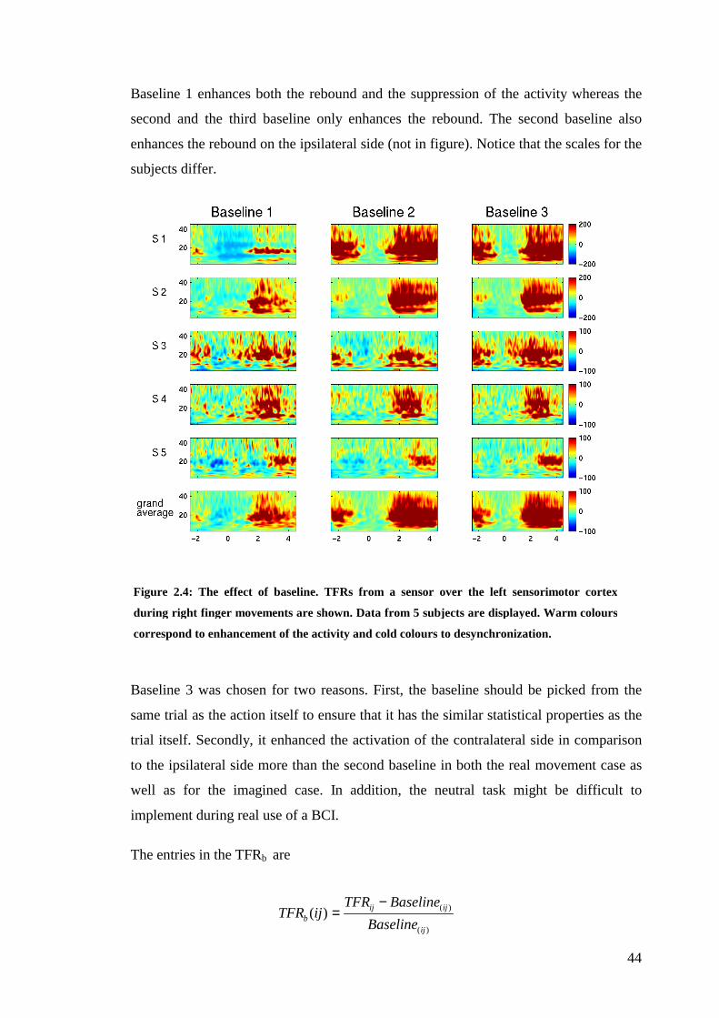
44
Baseline 1 enhances both the rebound and the suppression of the activity whereas the
second and the third baseline only enhances the rebound. The second baseline also
enhances the rebound on the ipsilateral side (not in figure). Notice that the scales for the
subjects differ.
Baseline 3 was chosen for two reasons. First, the baseline should be picked from the
same trial as the action itself to ensure that it has the similar statistical properties as the
trial itself. Secondly, it enhanced the activation of the contralateral side in comparison
to the ipsilateral side more than the second baseline in both the real movement case as
well as for the imagined case. In addition, the neutral task might be difficult to
implement during real use of a BCI.
The entries in the TFRb are
)(
)()(ij
ijijb Baseline
BaselineTFRijTFR
−=
Figure 2.4: The effect of baseline. TFRs from a sensor over the left sensorimotor cortex
during right finger movements are shown. Data from 5 subjects are displayed. Warm colours
correspond to enhancement of the activity and cold colours to desynchronization.
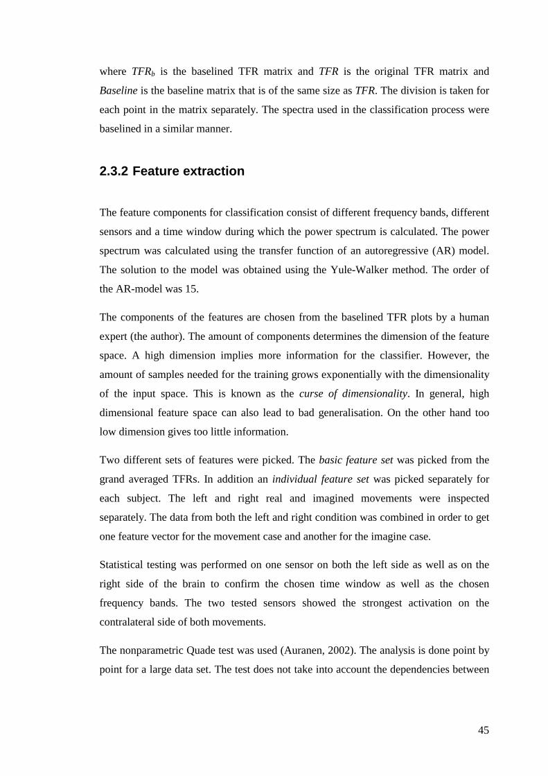
45
where TFRb is the baselined TFR matrix and TFR is the original TFR matrix and
Baseline is the baseline matrix that is of the same size as TFR. The division is taken for
each point in the matrix separately. The spectra used in the classification process were
baselined in a similar manner.
2.3.2 Feature extraction
The feature components for classification consist of different frequency bands, different
sensors and a time window during which the power spectrum is calculated. The power
spectrum was calculated using the transfer function of an autoregressive (AR) model.
The solution to the model was obtained using the Yule-Walker method. The order of
the AR-model was 15.
The components of the features are chosen from the baselined TFR plots by a human
expert (the author). The amount of components determines the dimension of the feature
space. A high dimension implies more information for the classifier. However, the
amount of samples needed for the training grows exponentially with the dimensionality
of the input space. This is known as the curse of dimensionality. In general, high
dimensional feature space can also lead to bad generalisation. On the other hand too
low dimension gives too little information.
Two different sets of features were picked. The basic feature set was picked from the
grand averaged TFRs. In addition an individual feature set was picked separately for
each subject. The left and right real and imagined movements were inspected
separately. The data from both the left and right condition was combined in order to get
one feature vector for the movement case and another for the imagine case.
Statistical testing was performed on one sensor on both the left side as well as on the
right side of the brain to confirm the chosen time window as well as the chosen
frequency bands. The two tested sensors showed the strongest activation on the
contralateral side of both movements.
The nonparametric Quade test was used (Auranen, 2002). The analysis is done point by
point for a large data set. The test does not take into account the dependencies between
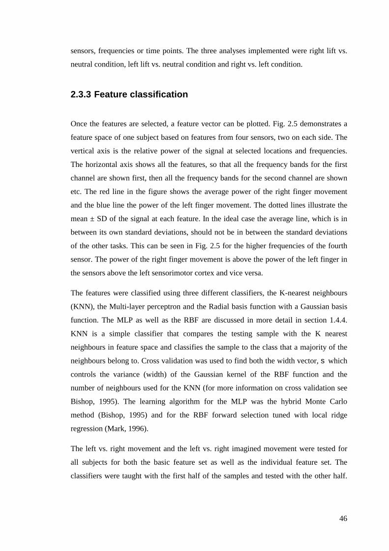
46
sensors, frequencies or time points. The three analyses implemented were right lift vs.
neutral condition, left lift vs. neutral condition and right vs. left condition.
2.3.3 Feature classification
Once the features are selected, a feature vector can be plotted. Fig. 2.5 demonstrates a
feature space of one subject based on features from four sensors, two on each side. The
vertical axis is the relative power of the signal at selected locations and frequencies.
The horizontal axis shows all the features, so that all the frequency bands for the first
channel are shown first, then all the frequency bands for the second channel are shown
etc. The red line in the figure shows the average power of the right finger movement
and the blue line the power of the left finger movement. The dotted lines illustrate the
mean ± SD of the signal at each feature. In the ideal case the average line, which is in
between its own standard deviations, should not be in between the standard deviations
of the other tasks. This can be seen in Fig. 2.5 for the higher frequencies of the fourth
sensor. The power of the right finger movement is above the power of the left finger in
the sensors above the left sensorimotor cortex and vice versa.
The features were classified using three different classifiers, the K-nearest neighbours
(KNN), the Multi-layer perceptron and the Radial basis function with a Gaussian basis
function. The MLP as well as the RBF are discussed in more detail in section 1.4.4.
KNN is a simple classifier that compares the testing sample with the K nearest
neighbours in feature space and classifies the sample to the class that a majority of the
neighbours belong to. Cross validation was used to find both the width vector, s which
controls the variance (width) of the Gaussian kernel of the RBF function and the
number of neighbours used for the KNN (for more information on cross validation see
Bishop, 1995). The learning algorithm for the MLP was the hybrid Monte Carlo
method (Bishop, 1995) and for the RBF forward selection tuned with local ridge
regression (Mark, 1996).
The left vs. right movement and the left vs. right imagined movement were tested for
all subjects for both the basic feature set as well as the individual feature set. The
classifiers were taught with the first half of the samples and tested with the other half.
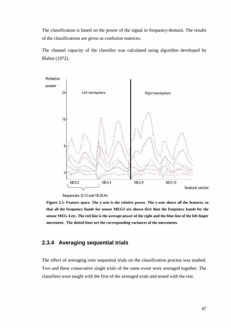
47
The classification is based on the power of the signal in frequency-domain. The results
of the classifications are given as confusion matrices.
The channel capacity of the classifier was calculated using algorithm developed by
Blahut (1972).
2.3.4 Averaging sequential trials
The effect of averaging over sequential trials on the classification process was studied.
Two and three consecutive single trials of the same event were averaged together. The
classifiers were taught with the first of the averaged trials and tested with the rest.
Figure 2.5: Feature space. The y-axis is the relative power. The y-axis shows all the features, so
that all the frequency bands for sensor MEG3 are shown first then the frequency bands for the
sensor MEG 4 etc. The red line is the average power of the right and the blue line of the left finger
movement. The dotted lines are the corresponding variances of the movements.
Relative
power
frequencies: 8-12 and 18-26 Hz
feature vector
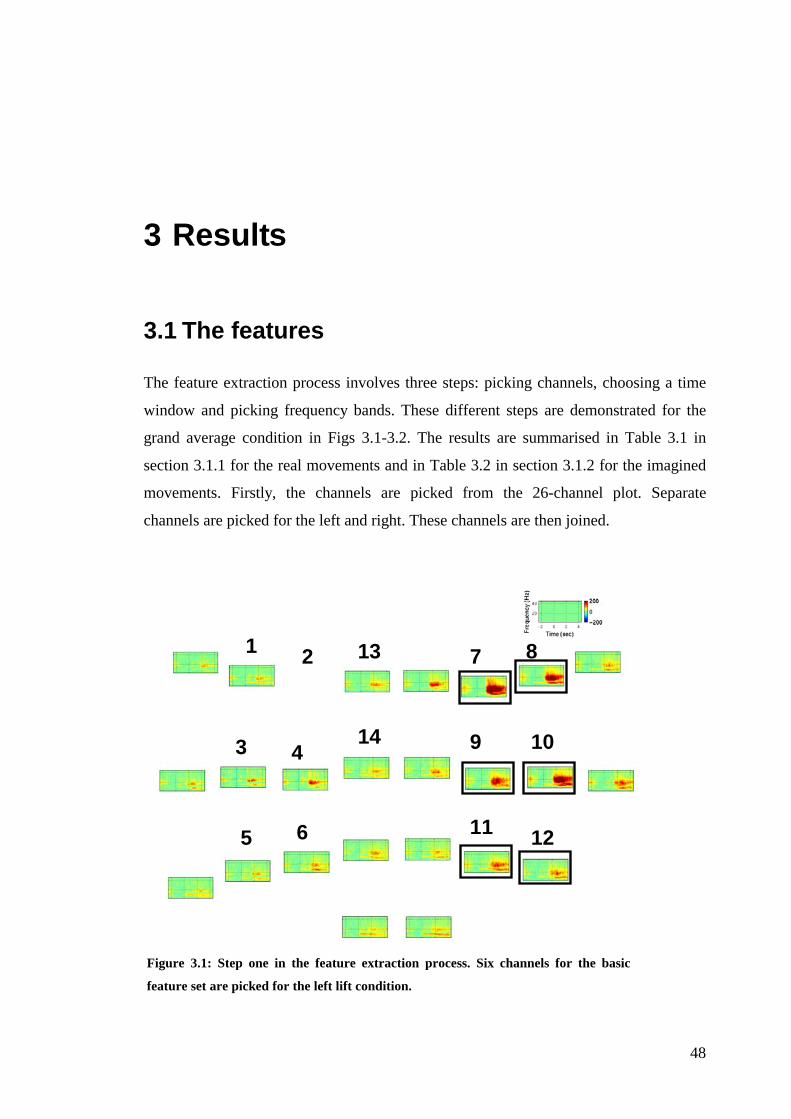
48
3 Results
3.1 The features
The feature extraction process involves three steps: picking channels, choosing a time
window and picking frequency bands. These different steps are demonstrated for the
grand average condition in Figs 3.1-3.2. The results are summarised in Table 3.1 in
section 3.1.1 for the real movements and in Table 3.2 in section 3.1.2 for the imagined
movements. Firstly, the channels are picked from the 26-channel plot. Separate
channels are picked for the left and right. These channels are then joined.
condition.
1 2
3 4
5 6
7 8
9 10
11 12
13
14
1 2
3 4
5 6
7 8
9 10
11 12
13
14
Figure 3.1: Step one in the feature extraction process. Six channels for the basic
feature set are picked for the left lift condition.
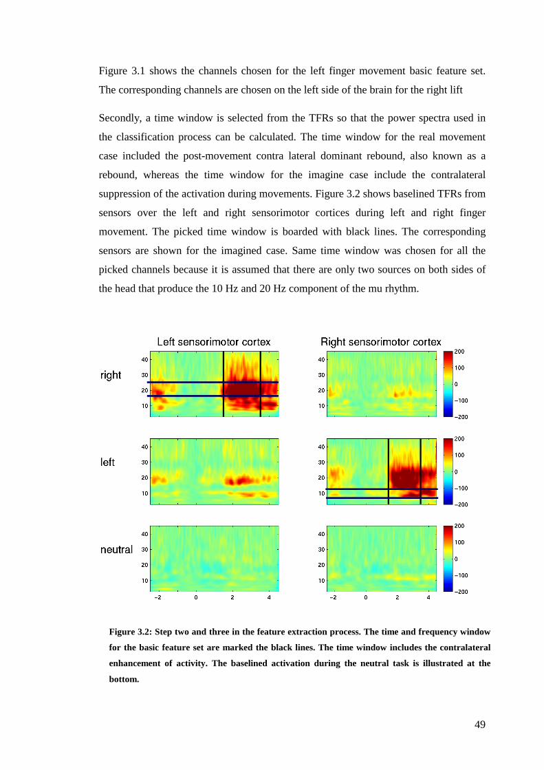
49
Figure 3.1 shows the channels chosen for the left finger movement basic feature set.
The corresponding channels are chosen on the left side of the brain for the right lift
Secondly, a time window is selected from the TFRs so that the power spectra used in
the classification process can be calculated. The time window for the real movement
case included the post-movement contra lateral dominant rebound, also known as a
rebound, whereas the time window for the imagine case include the contralateral
suppression of the activation during movements. Figure 3.2 shows baselined TFRs from
sensors over the left and right sensorimotor cortices during left and right finger
movement. The picked time window is boarded with black lines. The corresponding
sensors are shown for the imagined case. Same time window was chosen for all the
picked channels because it is assumed that there are only two sources on both sides of
the head that produce the 10 Hz and 20 Hz component of the mu rhythm.
Figure 3.1 Step 1 in the feature extraction process. Six channels for the basic feature set are
picked for the left lift condition.
Figure 3.2: Step two and three in the feature extraction process. The time and frequency window
for the basic feature set are marked the black lines. The time window includes the contralateral
enhancement of activity. The baselined activation during the neutral task is illustrated at the
bottom.
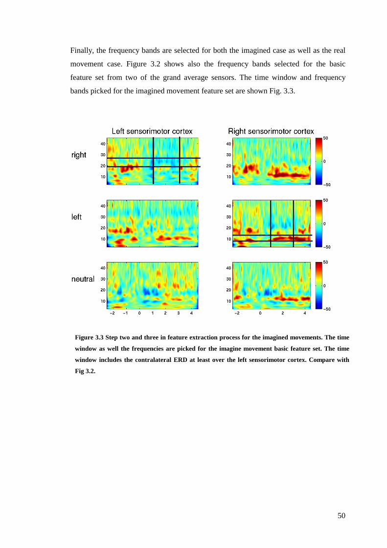
50
Finally, the frequency bands are selected for both the imagined case as well as the real
movement case. Figure 3.2 shows also the frequency bands selected for the basic
feature set from two of the grand average sensors. The time window and frequency
bands picked for the imagined movement feature set are shown Fig. 3.3.
Figure 3.2: Step two and three in the feature extraction process. The time window and the
frequency bands are picked for the basic feature set for both the left and right lift condition. The
time window has to be the same for both cases. The time window includes the contralateral ERS.
The baselined activation during the neutral task is illustrated at the bottom.
Figure 3.3 Step two and three in feature extraction process for the imagined movements. The time
window as well the frequencies are picked for the imagine movement basic feature set. The time
window includes the contralateral ERD at least over the left sensorimotor cortex. Compare with
Fig 3.2.
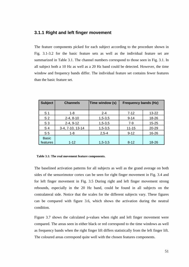
51
3.1.1 Right and left finger movement
The feature components picked for each subject according to the procedure shown in
Fig. 3.1-3.2 for the basic feature sets as well as the individual feature set are
summarized in Table 3.1. The channel numbers correspond to those seen in Fig. 3.1. In
all subject both a 10 Hz as well as a 20 Hz band could be detected. However, the time
window and frequency bands differ. The individual feature set contains fewer features
than the basic feature set.
The baselined activation patterns for all subjects as well as the grand average on both
sides of the sensorimotor cortex can be seen for right finger movement in Fig. 3.4 and
for left finger movement in Fig. 3.5 During right and left finger movement strong
rebounds, especially in the 20 Hz band, could be found in all subjects on the
contralateral side. Notice that the scales for the different subjects vary. These figures
can be compared with figure 3.6, which shows the activation during the neutral
condition.
Figure 3.7 shows the calculated p-values when right and left finger movement were
compared. The areas seen in either black or red correspond to the time windows as well
as frequency bands when the right finger lift differs statistically from the left finger lift.
The coloured areas correspond quite well with the chosen features components.
Subject Channels Time window (s) Frequency bands (Hz)
S 1 1-8 2-4 7-12 13-22
S 2 2-4, 8-10 1,5-3,5 9-14 18-26
S 3 2-4, 9-12 1,5-3,5 7-9 15-25
S 4 3-4, 7-10, 13-14 1,5-3,5 11-15 20-29
S 5 1-8 2,5-4 9-12 16-26
Basicfeatures 1-12 1,5-3,5 8-12 18-26
Table 3.1: The real movement feature components.
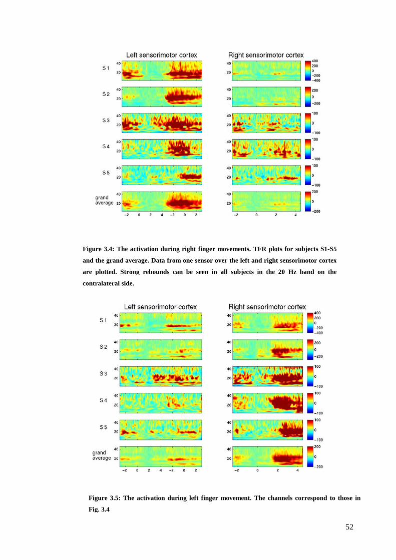
52
Figure 3.4: The activation during right finger movements. TFR plots for subjects S1-S5
and the grand average. Data from one sensor over the left and right sensorimotor cortex
are plotted. Strong rebounds can be seen in all subjects in the 20 Hz band on the
contralateral side.
Figure 3.5: The activation during left finger movement. The channels correspond to those in
Fig. 3.4
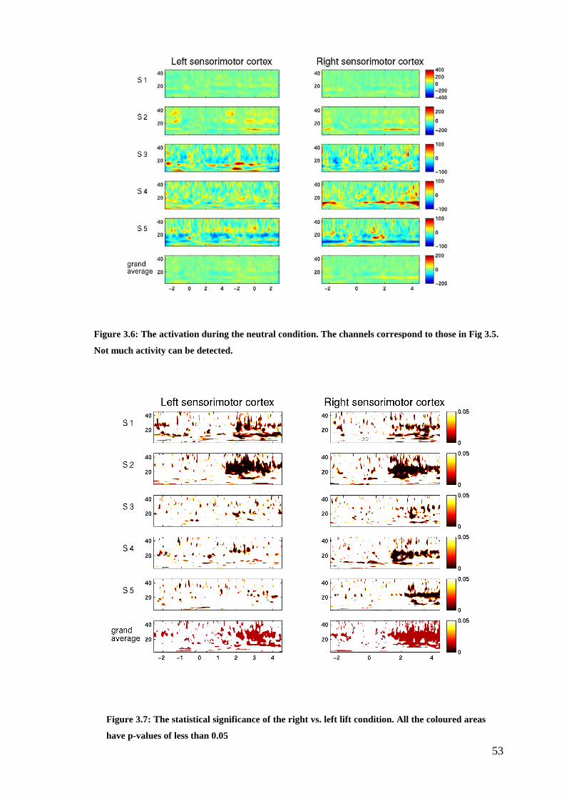
53
Figure 3.6: The activation during the neutral condition. The channels correspond to those in Fig 3.5.
Not much activity can be detected.
Figure 3.7: The statistical significance of the right vs. left lift condition. All the coloured areas
have p-values of less than 0.05

54
3.1.2 Imagined right and left finger movement
The features components picked for the imagined movements can be found in Table
3.2. Also the basic feature set picked from the grand average plots can be seen in the
same table. The channel numbers correspond to those seen in Fig. 3.1. The individual
feature set contains fewer features than the basic feature set.
The features picked are based on the contralateral suppression of the signal that should
occur while the subject is imagining the movement. However, as can be seen from Fig.
3.8 and 3.9 not all subjects show the contralateral dominant suppression. Subject S1
shows a strong contralateral suppression of the activation especially during imagination
of right finger movements in both the 10 Hz and 20 Hz bands. A less prominent
desynchronization can be detected also in S2. No significant desynchronization can be
detected in subjects S3-S4. Notice that the scales between subjects vary.
Figures 3.8 and 3.9 can also be compared with Fig. 3.6, which shows the activation of
the cortex when subjects are instructed to do nothing. Notice that activation during
imagination of movements do not differ from baseline level very much whereas the
activation during real movements and the neutral condition are 2 to 5 times larger or
smaller than the activation of the baseline.
Subject Channels Time window (s) Frequency bands (Hz)
S 1 2-4, 8-10 0.5-2-5 9-14 22-29S 2 1-8 0-1 9-15 20-25S 3 1-8 0-1.5 8-12 19-23S 4 1-4, 7, 8, 10 0.5-2 7-12 18-26S 5 1-8 0.5-2 11-15 19-26
Basicfeatures 1-12 0.5-2.5 9-15 20-26
Table 3.2: The features for the imagined movements.
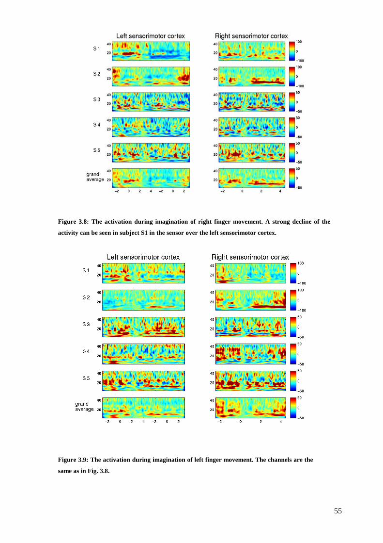
55
Figure 3.8: The activation during imagination of right finger movement. A strong decline of the
activity can be seen in subject S1 in the sensor over the left sensorimotor cortex.
Figure 3.9: The activation during imagination of left finger movement. The channels are the
same as in Fig. 3.8.
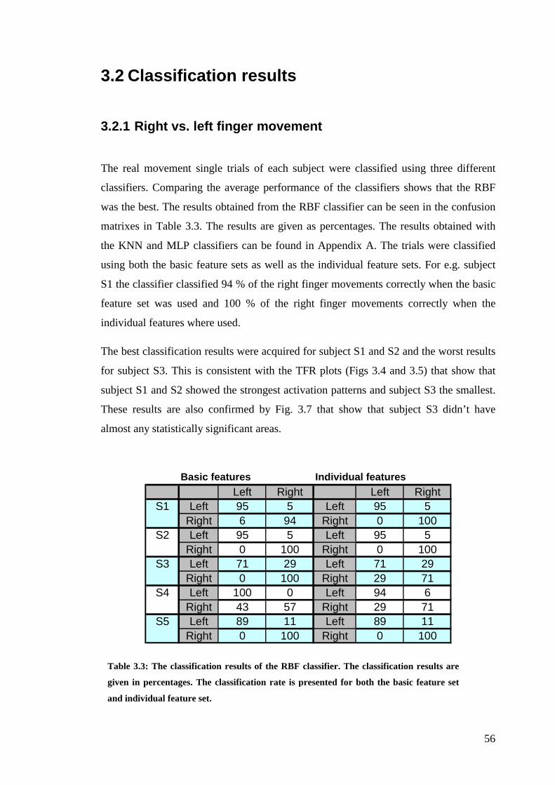
56
3.2 Classification results
3.2.1 Right vs. left finger movement
The real movement single trials of each subject were classified using three different
classifiers. Comparing the average performance of the classifiers shows that the RBF
was the best. The results obtained from the RBF classifier can be seen in the confusion
matrixes in Table 3.3. The results are given as percentages. The results obtained with
the KNN and MLP classifiers can be found in Appendix A. The trials were classified
using both the basic feature sets as well as the individual feature sets. For e.g. subject
S1 the classifier classified 94 % of the right finger movements correctly when the basic
feature set was used and 100 % of the right finger movements correctly when the
individual features where used.
The best classification results were acquired for subject S1 and S2 and the worst results
for subject S3. This is consistent with the TFR plots (Figs 3.4 and 3.5) that show that
subject S1 and S2 showed the strongest activation patterns and subject S3 the smallest.
These results are also confirmed by Fig. 3.7 that show that subject S3 didn’t have
almost any statistically significant areas.
Basic features Individual features
Left Right Left RightS1 Left 95 5 Left 95 5
Right 6 94 Right 0 100S2 Left 95 5 Left 95 5
Right 0 100 Right 0 100S3 Left 71 29 Left 71 29
Right 0 100 Right 29 71S4 Left 100 0 Left 94 6
Right 43 57 Right 29 71S5 Left 89 11 Left 89 11
Right 0 100 Right 0 100
Table 3.3: The classification results of the RBF classifier. The classification results are
given in percentages. The classification rate is presented for both the basic feature set
and individual feature set.
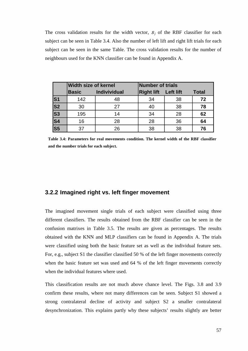
57
The cross validation results for the width vector, sj of the RBF classifier for each
subject can be seen in Table 3.4. Also the number of left lift and right lift trials for each
subject can be seen in the same Table. The cross validation results for the number of
neighbours used for the KNN classifier can be found in Appendix A.
3.2.2 Imagined right vs. left finger movement
The imagined movement single trials of each subject were classified using three
different classifiers. The results obtained from the RBF classifier can be seen in the
confusion matrixes in Table 3.5. The results are given as percentages. The results
obtained with the KNN and MLP classifiers can be found in Appendix A. The trials
were classified using both the basic feature set as well as the individual feature sets.
For, e.g., subject S1 the classifier classified 50 % of the left finger movements correctly
when the basic feature set was used and 64 % of the left finger movements correctly
when the individual features where used.
This classification results are not much above chance level. The Figs. 3.8 and 3.9
confirm these results, where not many differences can be seen. Subject S1 showed a
strong contralateral decline of activity and subject S2 a smaller contralateral
desynchronization. This explains partly why these subjects’ results slightly are better
Width size of kernel Number of trials Basic Indivividual Right lift Left lift Total
S1 142 48 34 38 72S2 30 27 40 38 78S3 195 14 34 28 62S4 16 28 28 36 64S5 37 26 38 38 76
Table 3.4: Parameters for real movements condition. The kernel width of the RBF classifier
and the number trials for each subject.
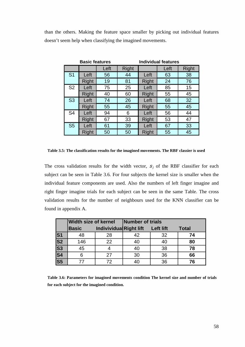
58
than the others. Making the feature space smaller by picking out individual features
doesn’t seem help when classifying the imagined movements.
The cross validation results for the width vector, sj of the RBF classifier for each
subject can be seen in Table 3.6. For four subjects the kernel size is smaller when the
individual feature components are used. Also the numbers of left finger imagine and
right finger imagine trials for each subject can be seen in the same Table. The cross
validation results for the number of neighbours used for the KNN classifier can be
found in appendix A.
Width size of kernel Number of trials Basic IndivividualRight lift Left lift Total
S1 48 28 42 32 74S2 146 22 40 40 80S3 45 4 40 38 78S4 6 27 30 36 66S5 77 72 40 36 76
Table 3.5: The classification results for the imagined movements. The RBF classier is used
Table 3.6: Parameters for imagined movements condition The kernel size and number of trials
for each subject for the imagined condition.
Basic features Individual features
Left Right Left RightS1 Left 56 44 Left 63 38
Right 19 81 Right 24 76S2 Left 75 25 Left 85 15
Right 40 60 Right 55 45S3 Left 74 26 Left 68 32
Right 55 45 Right 55 45S4 Left 94 6 Left 56 44
Right 67 33 Right 53 47S5 Left 61 39 Left 67 33
Right 50 50 Right 55 45
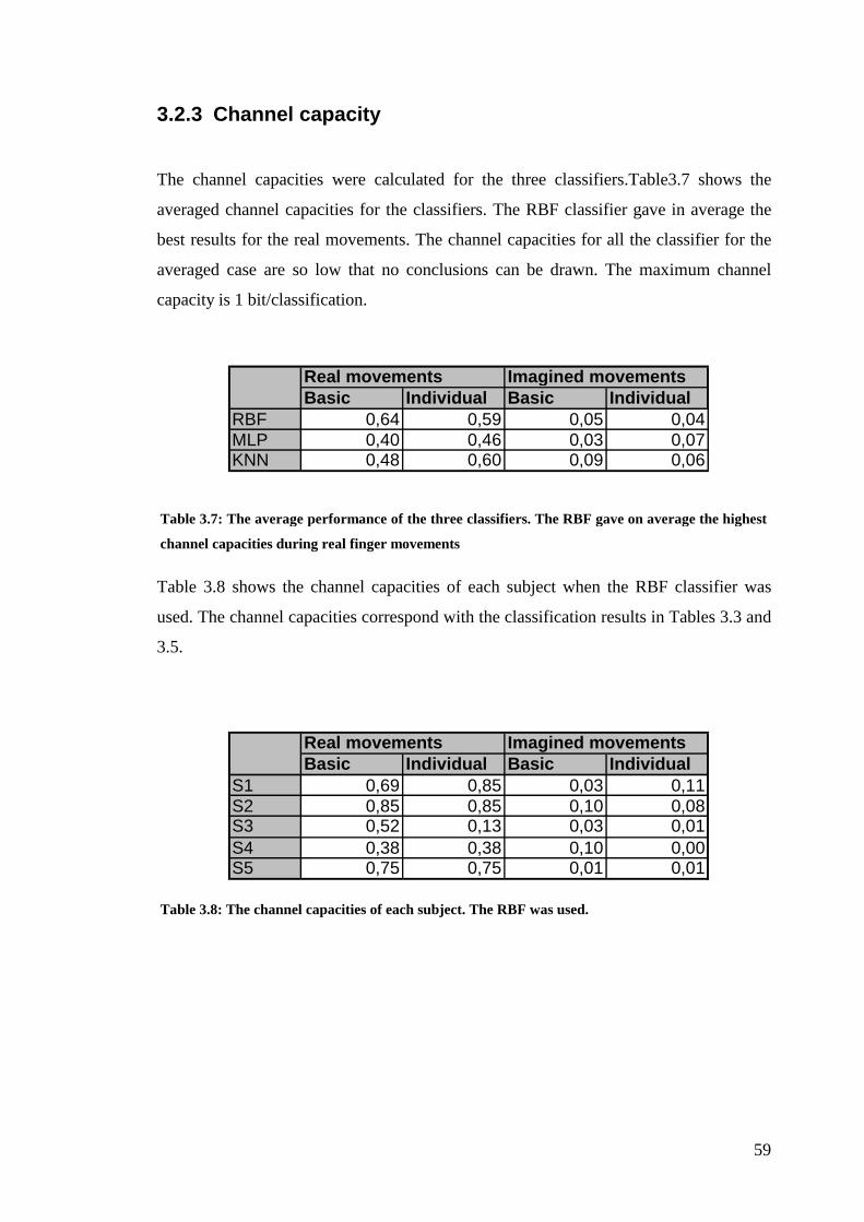
59
3.2.3 Channel capacity
The channel capacities were calculated for the three classifiers.Table3.7 shows the
averaged channel capacities for the classifiers. The RBF classifier gave in average the
best results for the real movements. The channel capacities for all the classifier for the
averaged case are so low that no conclusions can be drawn. The maximum channel
capacity is 1 bit/classification.
Table 3.8 shows the channel capacities of each subject when the RBF classifier was
used. The channel capacities correspond with the classification results in Tables 3.3 and
3.5.
Table 3.7: The average performance of the three classifiers. The RBF gave on average the highest
channel capacities during real finger movements
Table 3.8: The channel capacities of each subject. The RBF was used.
Real movements Imagined movementsBasic Individual Basic Individual
RBF 0,64 0,59 0,05 0,04MLP 0,40 0,46 0,03 0,07KNN 0,48 0,60 0,09 0,06
Real movements Imagined movementsBasic Individual Basic Individual
S1 0,69 0,85 0,03 0,11S2 0,85 0,85 0,10 0,08S3 0,52 0,13 0,03 0,01S4 0,38 0,38 0,10 0,00S5 0,75 0,75 0,01 0,01
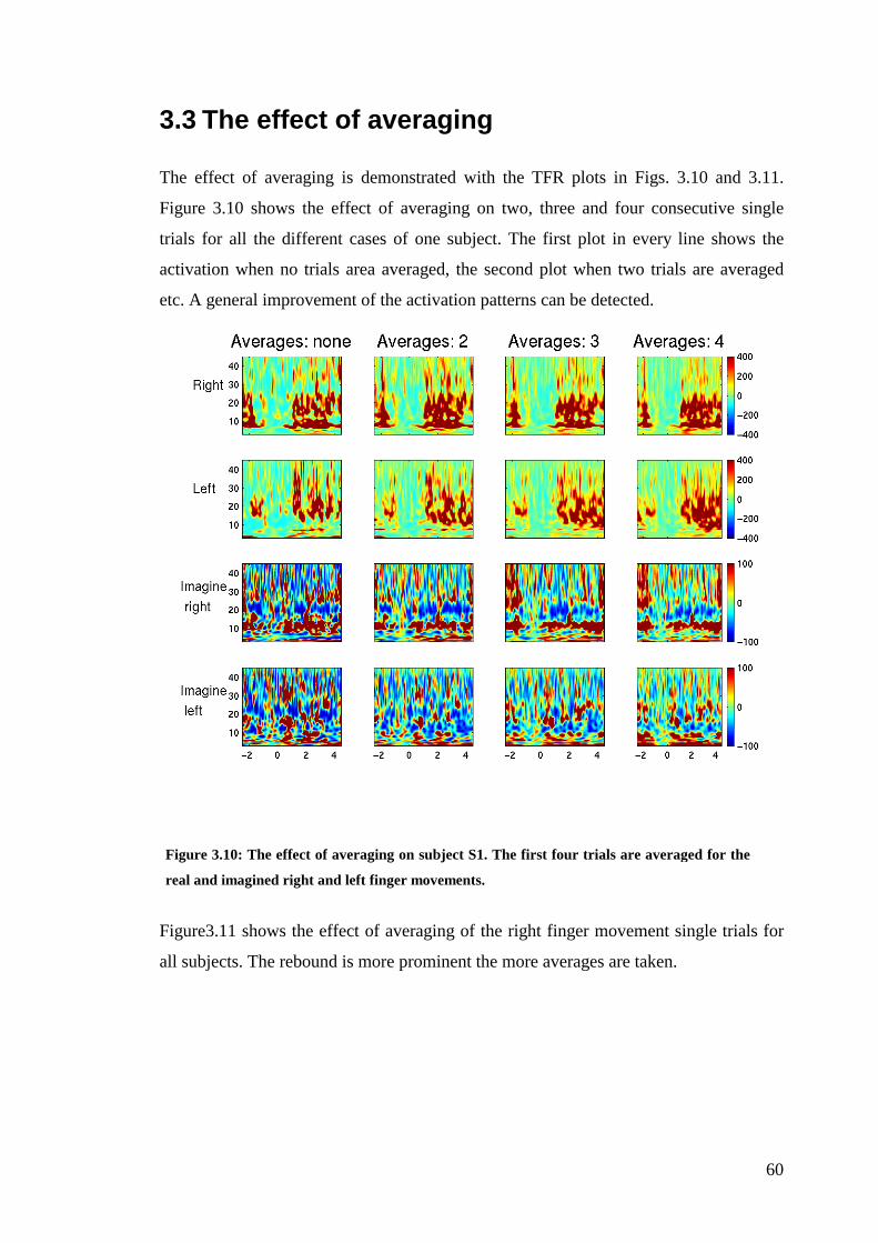
60
3.3 The effect of averaging
The effect of averaging is demonstrated with the TFR plots in Figs. 3.10 and 3.11.
Figure 3.10 shows the effect of averaging on two, three and four consecutive single
trials for all the different cases of one subject. The first plot in every line shows the
activation when no trials area averaged, the second plot when two trials are averaged
etc. A general improvement of the activation patterns can be detected.
Figure3.11 shows the effect of averaging of the right finger movement single trials for
all subjects. The rebound is more prominent the more averages are taken.
Figure 3.10: The effect of averaging on subject S1. The first four trials are averaged for the
real and imagined right and left finger movements.
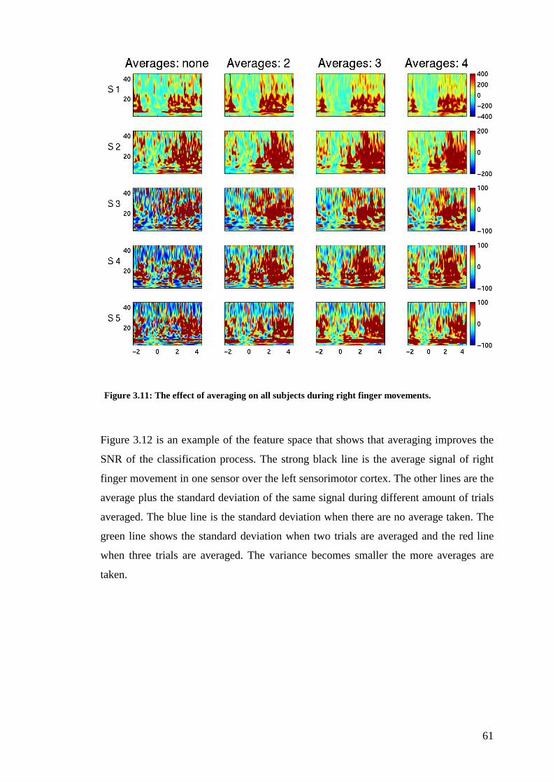
61
Figure 3.12 is an example of the feature space that shows that averaging improves the
SNR of the classification process. The strong black line is the average signal of right
finger movement in one sensor over the left sensorimotor cortex. The other lines are the
average plus the standard deviation of the same signal during different amount of trials
averaged. The blue line is the standard deviation when there are no average taken. The
green line shows the standard deviation when two trials are averaged and the red line
when three trials are averaged. The variance becomes smaller the more averages are
taken.
Figure 3.11: The effect of averaging on all subjects during right finger movements.
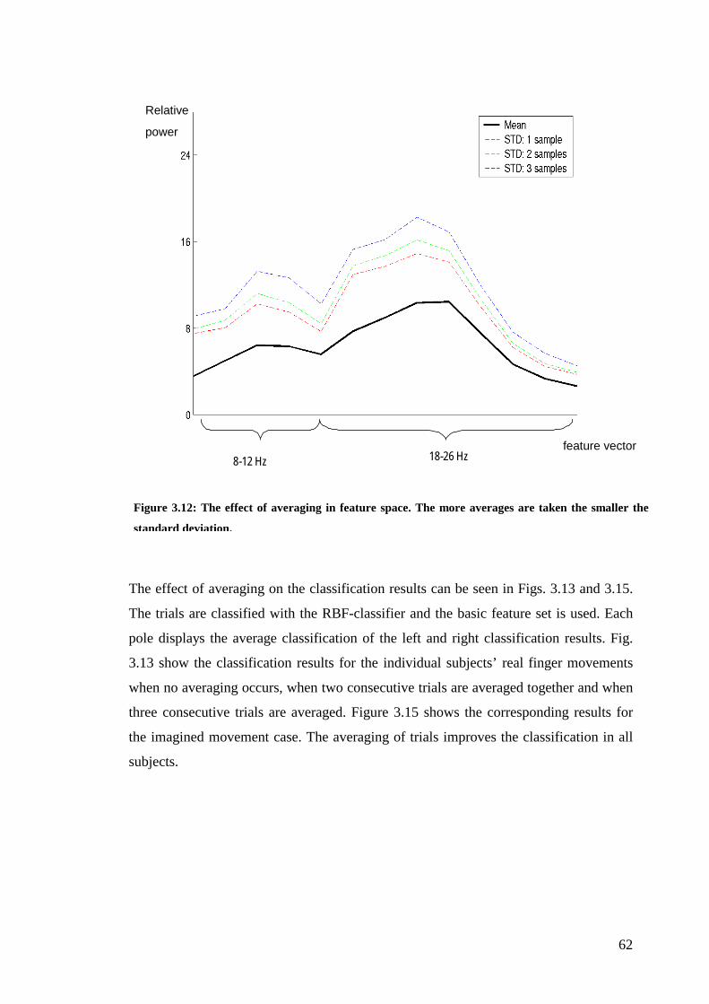
62
The effect of averaging on the classification results can be seen in Figs. 3.13 and 3.15.
The trials are classified with the RBF-classifier and the basic feature set is used. Each
pole displays the average classification of the left and right classification results. Fig.
3.13 show the classification results for the individual subjects’ real finger movements
when no averaging occurs, when two consecutive trials are averaged together and when
three consecutive trials are averaged. Figure 3.15 shows the corresponding results for
the imagined movement case. The averaging of trials improves the classification in all
subjects.
Figure 3.12: The effect of averaging in feature space. The more averages are taken the smaller the
standard deviation.
Relative
power
18-26 Hz8-12 Hzfeature vector
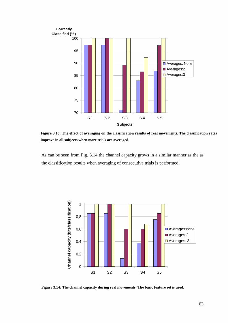
63
As can be seen from Fig. 3.14 the channel capacity grows in a similar manner as the as
the classification results when averaging of consecutive trials is performed.
Figure 3.14: The channel capacity during real movements. The basic feature set is used.
Figure 3.13: The effect of averaging on the classification results of real movements. The classification rates
improve in all subjects when more trials are averaged.
70
75
80
85
90
95
100
S 1 S 2 S 3 S 4 S 5
Subjects
Correctly Classified (%)
Averages: None
Averages:2
Averages:3
0
0,2
0,4
0,6
0,8
1
S1 S2 S3 S4 S5
Ch
ann
el c
apac
ity (b
its/c
lass
ifica
tion
)
Averages:none
Averages:2
Averages: 3
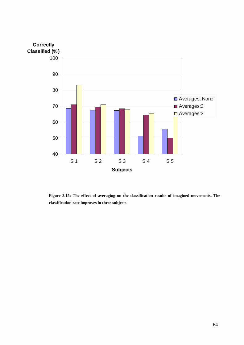
64
Figure 3.15: The effect of averaging on the classification results of imagined movements. The
classification rate improves in three subjects
40
50
60
70
80
90
100
S 1 S 2 S 3 S 4 S 5
Subjects
Correctly Classified (%)
Averages: None
Averages:2
Averages:3
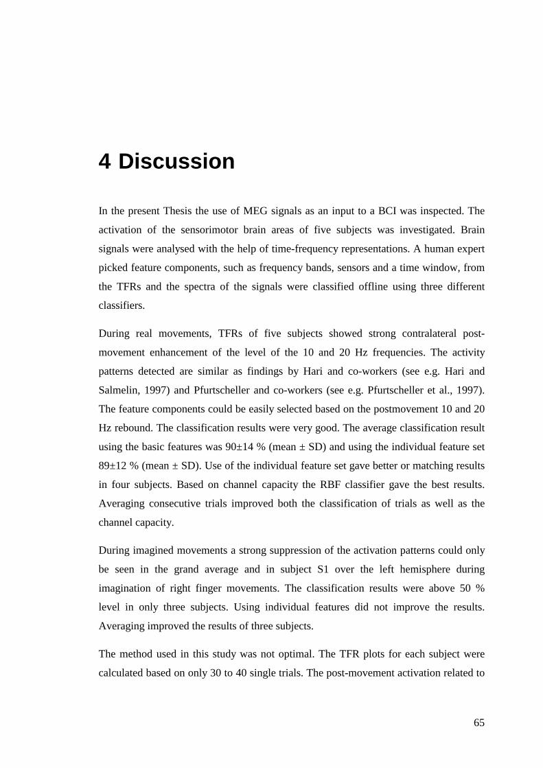
65
4 Discussion
In the present Thesis the use of MEG signals as an input to a BCI was inspected. The
activation of the sensorimotor brain areas of five subjects was investigated. Brain
signals were analysed with the help of time-frequency representations. A human expert
picked feature components, such as frequency bands, sensors and a time window, from
the TFRs and the spectra of the signals were classified offline using three different
classifiers.
During real movements, TFRs of five subjects showed strong contralateral post-
movement enhancement of the level of the 10 and 20 Hz frequencies. The activity
patterns detected are similar as findings by Hari and co-workers (see e.g. Hari and
Salmelin, 1997) and Pfurtscheller and co-workers (see e.g. Pfurtscheller et al., 1997).
The feature components could be easily selected based on the postmovement 10 and 20
Hz rebound. The classification results were very good. The average classification result
using the basic features was 90±14 % (mean ± SD) and using the individual feature set
89±12 % (mean ± SD). Use of the individual feature set gave better or matching results
in four subjects. Based on channel capacity the RBF classifier gave the best results.
Averaging consecutive trials improved both the classification of trials as well as the
channel capacity.
During imagined movements a strong suppression of the activation patterns could only
be seen in the grand average and in subject S1 over the left hemisphere during
imagination of right finger movements. The classification results were above 50 %
level in only three subjects. Using individual features did not improve the results.
Averaging improved the results of three subjects.
The method used in this study was not optimal. The TFR plots for each subject were
calculated based on only 30 to 40 single trials. The post-movement activation related to
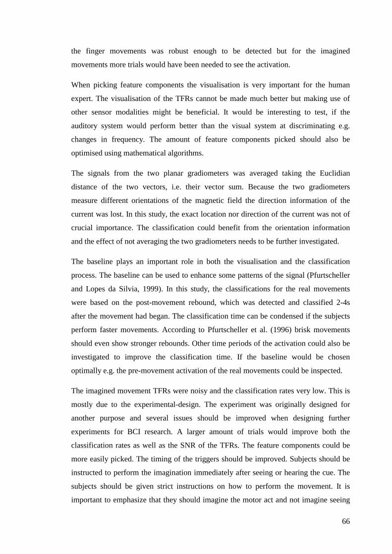
66
the finger movements was robust enough to be detected but for the imagined
movements more trials would have been needed to see the activation.
When picking feature components the visualisation is very important for the human
expert. The visualisation of the TFRs cannot be made much better but making use of
other sensor modalities might be beneficial. It would be interesting to test, if the
auditory system would perform better than the visual system at discriminating e.g.
changes in frequency. The amount of feature components picked should also be
optimised using mathematical algorithms.
The signals from the two planar gradiometers was averaged taking the Euclidian
distance of the two vectors, i.e. their vector sum. Because the two gradiometers
measure different orientations of the magnetic field the direction information of the
current was lost. In this study, the exact location nor direction of the current was not of
crucial importance. The classification could benefit from the orientation information
and the effect of not averaging the two gradiometers needs to be further investigated.
The baseline plays an important role in both the visualisation and the classification
process. The baseline can be used to enhance some patterns of the signal (Pfurtscheller
and Lopes da Silvia, 1999). In this study, the classifications for the real movements
were based on the post-movement rebound, which was detected and classified 2-4s
after the movement had began. The classification time can be condensed if the subjects
perform faster movements. According to Pfurtscheller et al. (1996) brisk movements
should even show stronger rebounds. Other time periods of the activation could also be
investigated to improve the classification time. If the baseline would be chosen
optimally e.g. the pre-movement activation of the real movements could be inspected.
The imagined movement TFRs were noisy and the classification rates very low. This is
mostly due to the experimental-design. The experiment was originally designed for
another purpose and several issues should be improved when designing further
experiments for BCI research. A larger amount of trials would improve both the
classification rates as well as the SNR of the TFRs. The feature components could be
more easily picked. The timing of the triggers should be improved. Subjects should be
instructed to perform the imagination immediately after seeing or hearing the cue. The
subjects should be given strict instructions on how to perform the movement. It is
important to emphasize that they should imagine the motor act and not imagine seeing

67
the movement because different cortical areas are involved in these two processes
(Crammond, 1997). The imagination of movements should be practised before the
subject enters the magnetically shielded room. The imagined movements should also be
short.
The present study showed that the activation patterns between subjects differ.
Especially the frequencies of the mu rhythm varied between subjects. High
classifications during real movements could be achieved with the feature components
picked from the grand average. Nonetheless, higher classification rate was obtained in
four of the subjects when the individual feature set was used, even though the
dimension of the feature space was lower. The grand average results suggest that when
a subject uses the BCI for the first time general features components can be used when
the classifier is taught. The feature components should be updated once new signals
have been recorded. The individual feature set did not improve the classification of the
imagined movements. This is mostly due to the fact that the individual TFRs were too
noisy and no individual feature components could be picked. Furthermore, the
individual feature set had a lower dimension and less information was given to the
classifier.
Another important difference between the subjects was the power of the activity. The
difference can be due to the head's distance from the sensors during the recordings
(magnetic field attenuates as 1/r2). When doing online BCI experiments its important to
make sure that the subjects are seated properly.
One important finding of this study was the positive effect of averaging on the
classification. During real movements hundred percent classification rates were
obtained in four subjects after averaging two or three trials. Nevertheless, the
classification rate did not improve in all subjects. It is not optimal to average trials
several minutes apart form each other because the statistical properties of the signal
might change. This is not an issue when using a BCI, because the triggers will be
presented only a couple seconds apart. The averaging did not improve the classification
rate of the imagined movements of the subjects with noisy signals probably due to the
fact that integrating noise just leads to more noise.
Even though averaging improves the SNR it also increases the time needed for the
classification. The time and amount of averages-trade-off, needs to be optimised. The
68
detected sensorimotor activity is presumably produced by two sources, one in
somatosensory cortex and another in the motor cortex (Salmelin and Hari, 1999).
Accordingly, sensors could be averaged spatially. If the sensors used for the averages
are picked well, the same effect should be obtained as when averaging over time.
In this Thesis real finger movements were inspected even though motor disabled cannot
conduct any motor behaviour and the healthy users can use their motor skills to execute
commands on a computer far more quicker than a noninvasive BCI. There were two
main reasons for this. Firstly, the activation of the sensorimotor cortex of paralysed and
other motor disabled patients is not very well defined. Some fMRI studies could be
found which showed that the activation when attempting to perform movements
resembled the activation of healthy people when performing real movements (see, e.g.,
Shoham et al., 2001). Secondly and most importantly, the results of the present study
for the real finger movements show that if the task of the subject is selected properly
and the feature space is well defined a robust classification can be achieved based on
just a few teaching trials.
Another aim of this work was to investigate the similarities of the activation patterns of
real movements and imagined movements. The features picked in this study for the two
cases were very different. This is mostly due to the different time courses of the
activation patterns studied. This study does not exclude the possibility of using real
movements to teach a robust classifier that could be used with imagined movements.
According to Pfurtscheller and Neuper (1997) the pre-movement suppression of the
activity of real movements should be similar to the suppression during imagination.
These similarities could not be studied in this Thesis due to the small amount of trials.
The use of both real movements and imagined movements in BCIs need to be further
investigated.
This study verifies that a human expert can provide the classifier a priori information
and help the classification process. However, the process of picking individual feature
sets for all future BCI users is very time-consuming. A mathematical pattern
recognition algorithm should be created to see if the process could be done with a
computer instead. It will be interesting to see if a computer performs better than the
human visual system at picking out important features. Presumably, the process will in
the future be interplay between the computer and a human expert.
69
The main aim of this Thesis was to study the use of MEG signals in BCIs. The results
are very encouraging. Parra et al. (2002) classified offline MEG signals. Their study
classified sensorimotor signals in time-domain. The signals over multiple sensors were
integrated. Better results were obtained in this Thesis with frequency-domain analysis.
Portin et al. (1996), classified offline frequency-domain signals using self-organizing
maps. When the maps were trained with features from the amplitude spectra 85 % of
the signals during movements were classified correctly. The use of the post-movement
rebound in this Thesis seems to work better. Portin et al. (1996) used more trials to train
the maps than the present study.
Most present BCI are either invasive or then based on EEG measurements. MEG
detects the signals more locally than EEG. The magnetic fields are not distorted by
tissue like the electrical fields. For BCI use the sensors showing the activation are
easily found and the feature set can be more easily picked with MEG. In addition, MEG
is less affected than EEG by the brain’s activity from other parts of the brain and the
radially located sources in the gyri. The SNR for the inspected phenomenon is higher.
SNR plays a very important role in single trial studies.
The three main problems using MEG in BCI research are its big size, its high price and
the fact that the MEG system has to be operated in a magnetically silent environment.
However, this Thesis was about basic research on BCIs and the technical problems will
not be thought of as barriers. New technologies evolve and a portable MEG device
might be a part of very day life in the future.
In conclusion, neuromagnetic sensorimotor oscillatory activity of finger movements
was successfully classified. This serves as a basis for future research. The method used
for pre-processing the data before classification influences the classification results. It
is important to define the task of the subjects properly, adjust the baseline to the
activation of interest and select the feature components with care. In addition,
averaging trials over time or space can improve the classification rate. The use of MEG
signals provides a new approach for BCIs, which needs to be further inspected.
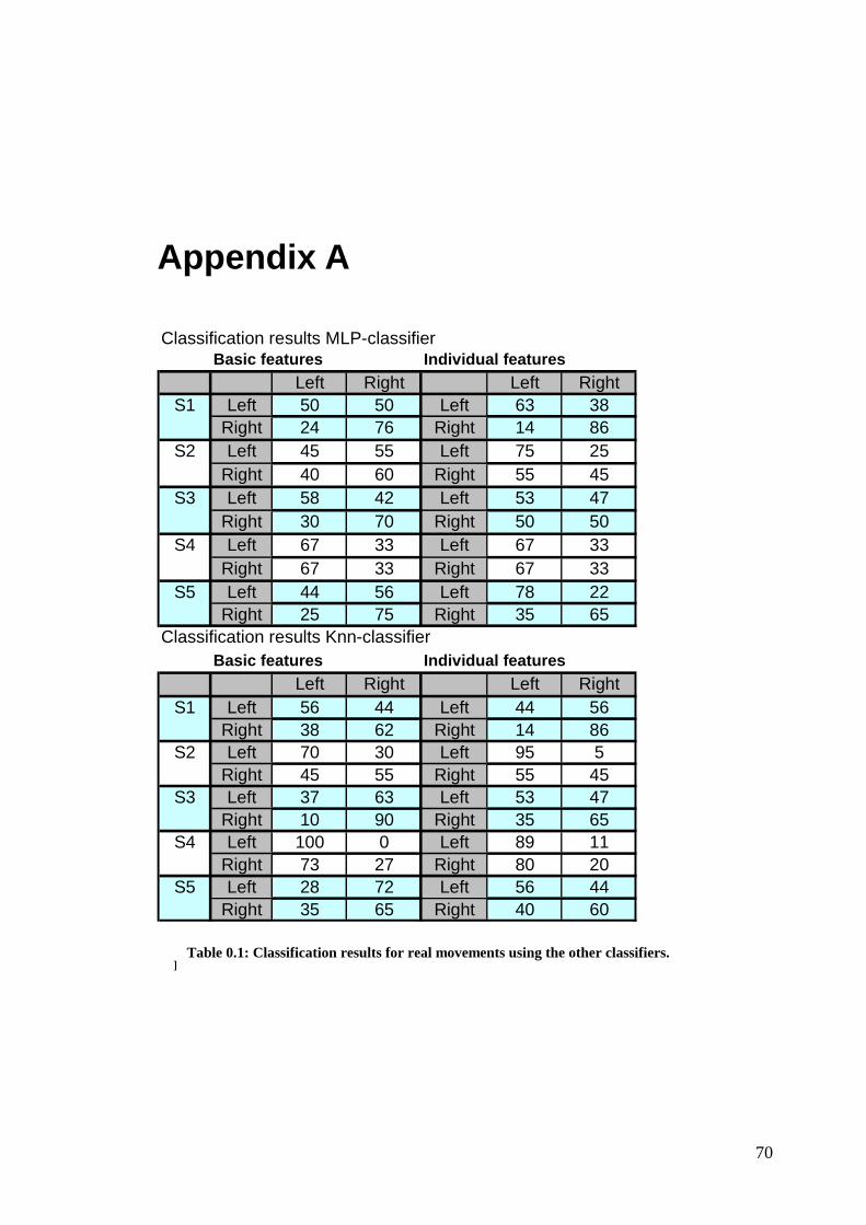
70
Appendix A
Classification results MLP-classifierBasic features Individual features
Left Right Left RightS1 Left 50 50 Left 63 38
Right 24 76 Right 14 86S2 Left 45 55 Left 75 25
Right 40 60 Right 55 45S3 Left 58 42 Left 53 47
Right 30 70 Right 50 50S4 Left 67 33 Left 67 33
Right 67 33 Right 67 33S5 Left 44 56 Left 78 22
Right 25 75 Right 35 65Classification results Knn-classifier
Basic features Individual featuresLeft Right Left Right
S1 Left 56 44 Left 44 56Right 38 62 Right 14 86
S2 Left 70 30 Left 95 5Right 45 55 Right 55 45
S3 Left 37 63 Left 53 47Right 10 90 Right 35 65
S4 Left 100 0 Left 89 11Right 73 27 Right 80 20
S5 Left 28 72 Left 56 44Right 35 65 Right 40 60
Figure A.1 Real movements Table 0.1: Classification results for real movements using the other classifiers.
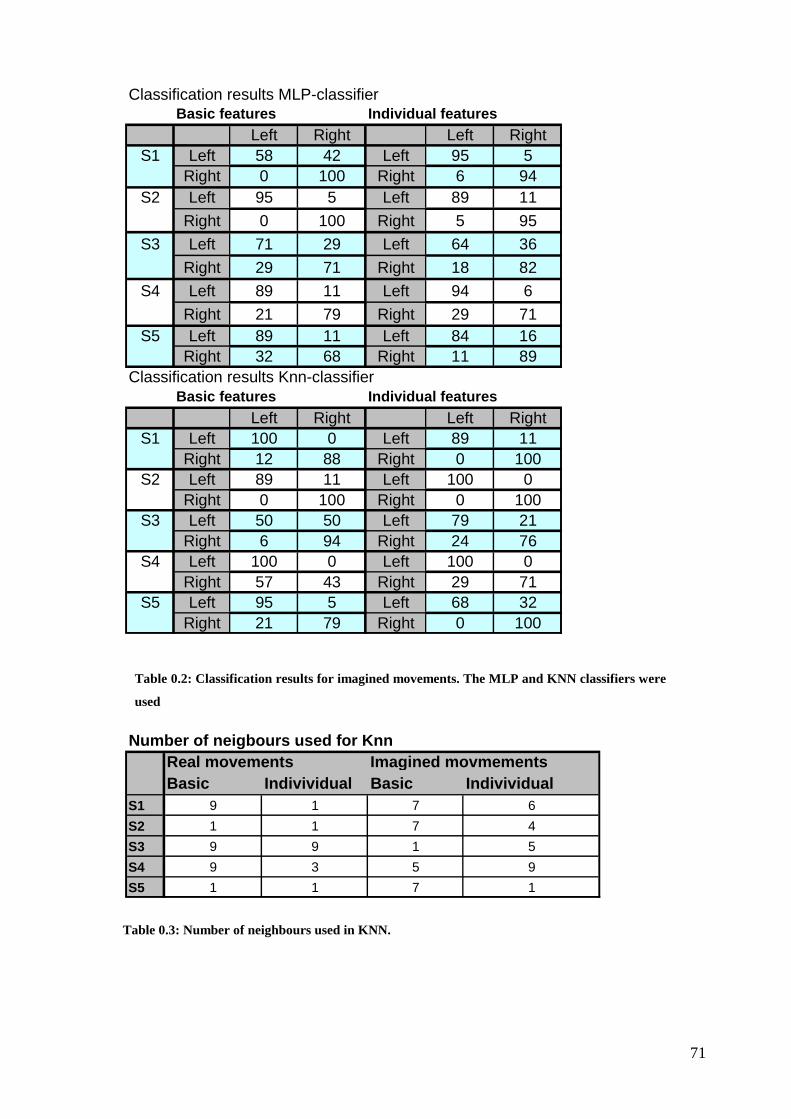
71
Classification results MLP-classifierBasic features Individual features
Left Right Left RightS1 Left 58 42 Left 95 5
Right 0 100 Right 6 94S2 Left 95 5 Left 89 11
Right 0 100 Right 5 95
S3 Left 71 29 Left 64 36
Right 29 71 Right 18 82
S4 Left 89 11 Left 94 6
Right 21 79 Right 29 71S5 Left 89 11 Left 84 16
Right 32 68 Right 11 89Classification results Knn-classifier
Basic features Individual features
Left Right Left RightS1 Left 100 0 Left 89 11
Right 12 88 Right 0 100S2 Left 89 11 Left 100 0
Right 0 100 Right 0 100S3 Left 50 50 Left 79 21
Right 6 94 Right 24 76S4 Left 100 0 Left 100 0
Right 57 43 Right 29 71S5 Left 95 5 Left 68 32
Right 21 79 Right 0 100
Table 0.2: Classification results for imagined movements. The MLP and KNN classifiers were
used
Number of neigbours used for KnnReal movements Imagined movmementsBasic Indivividual Basic Indivividual
S1 9 1 7 6
S2 1 1 7 4
S3 9 9 1 5
S4 9 3 5 9
S5 1 1 7 1
Table 0.3: Number of neighbours used in KNN.
72
References
Auranen T. (2002). Nonparametric statistical analysis of time-frequency
representations of magnetoencephalographic data, Master’s Thesis, Helsinki
University of Technology.
Baillet S., Mosher J. C., and Leahy R. M. (2001). Electromagnetic brain mapping,
IEEE Signal Processing Magazine, November, 14-30.
Birmbaumer N., Kubler A., Ghanayim N., Hinterberger T., Perelmouter J., Kaiser J.,
Iversen I., Kotchoubey B., Neumann N., and Flor H. (2000). The Thought Translation
Device for Completely Paralysed Patients, IEEE Transactions on rehabilitation
engineering, 8, 190-193.
Bishop C. M. (1995). Neural Networks for Pattern Recognition, Clarendon Press,
Oxford, 1st edition.
Blahut R. E. (1972). Computation of Channel Capacity and Rate-Distortion, IEEE
Transactions in Information Theory, 18, 4, 460-473.
Clark Jr J. W. (1995). The origin of biopotentials, Medical Instrumentation Application
and Design, Webster J. G (ed), John Wiley & Sons Inc, New York, 2nd edition,
Chapter 4, 150-227.
Crammond D. J. (1997). Motor imagery: never in your wildest dream, Trends in
Neuroscience, 20, (2), 54-57.
Donchin E., Spencer K. M., and Wijesinghe R. (2000). The mental prosthesis; assessing
the speed of a P300-based brain-computer interface, IEEE Transactions on
rehabilitation engineering, 8, (2), 174-179.
73
Elbert T. (1998) Neuromagnetism, Magnetism in medicine a handbook, Andrä W. and
Nowak H. (Eds), GAM media GmbH, Berlin, 1st Edition, Chapter 2.4, 190-261.
Gerloff C., Richard J., Hadley J., Schulman A. E. Honda M., and Hallett M. (1998).
Functional coupling and regional activation of human cortical motor areas during
simple, internally paced and externally paced finger movements, Brain, 121, 1513-
1531.
Geyer S., Matelli M., Luppino G., and Zilles K. (2000). Functional neuroanatomy of
the primate isocortical motor system, Anatomical Embryology, 202, 443-474.
Glaser R. (2001). Biophysics, Springer-Verlag Berlin, Heidelberg, 4th edition, 159-160.
Hari R. (1999). Magnetoencephalography as a tool of clinical neurophysiology,
Electroencephalography, Basic Principles, Clinical Applications, and Related Fields,
Niedermeyer E. and Lopes da Silva F. (Eds), Williams and Wilkins, Baltimore, 4th
edition, Chapter 60, 1107-1134.
Hari R. and Ilmoniemi R. (1986). Cerebral magnetic fields, Critical Review of
Biomedical Engineering, 14, (2), 93-126.
Hari R. and Salmelin R. (1997). Human cortical oscillations: a neuromagnetic view
through the skull, Trends in Neuroscience, 20, (1), 44-49.
Hari R. and Salenius S. (1999). Rhythmical corticomotor communication,
NeuroReport, 10, R1-R10.
Hari R., Salmelin R., Mäkelä JP., Salenius S., and Helle M. (1997).
Magnetoencephalographic cortical rhythms, International Journal of
Psychophysiology, 26, (1-3), 51-62.
Haykin S. (1999). Neural Networks a Comprehensive Foundation, Prentice-Hall Inc,
New Jersey, 2nd edition, 1-53.
Hyvärinen J. (1977). Neurobiologia, Tammi, Helsinki, 1-100.
Hämäläinen M., Hari R., Ilmoniemi R. J., Knuuttila J., and Lounasmaa O. V. (1993).
Magnetoencephalography – theory, instrumentation, and applications to noninvasive
studies of the working human brain, Reviews of Modern Physics, 65, (2), 413-497.
74
Jeannerod M. (1994). Mental imagery in the motor context, Neuropsychologia, 33,
(11), 1419-1432.
Jensen, O. (2000). 4-D Toolbox, version 1.1/1.2. A Matlab toolbox for the analysis of
Neuromag data. Http://boojum.hut.fi/~ojensen/4Dtools/.
Kaiser J., Lutzenberger W., Preissl H., Mosshammer D., and Birmbaumer N. (2000).
Statistical probability mapping reveals high-frequency magnetoencephalographic
activity in supplementary motor area during self-paced finger movements,
Neuroscience Letters, 283, (1), 81-84.
Kakigi R., Hoshiyama M., Shimojo M., Naka. D., Yamasaki H., Watanabe S., Xiang J.,
Maeda K., Lam K., Itomi K., and Nakamura A. (2000). The somatosensory evoked
magnetic fields, Progress in Neurobiology, 61, 495-523.
Kandel E. R., Schwartz J. H., and Jessel T. M. (eds.) (1991). Priniciples of neural
science, Prentice Hall International, Inc., Connecticut, 3rd edition.
Lehtonen J. (2002). EEG-based Brain Computer Interfaces. Master’s Thesis, Helsinki
University of Technology.
Lindsay T. D. (1996). Functional Human Anatomy, Mosby-Year Book, St. Louis
Missouri.
Mark J. L. (1996). Introduction to Radial Basis Function Networks. Technical report by
Centre for Cognitive Science, University of Edinburgh.
Mikulis D. J. Jurkiewicz M. T., McIlroy W. E., Staines W. R., Rickards L., Kalsi-Ryan
S., Crawley A. P., Fehlings M. G., and Verrier M. C. (2002) Adaptation in the motor
cortex following cervical spinal cord injury, Neurology, 58, (5), 794-801.
Millan J., Mourino J., Marciani M., Babiloni F., Topani F., Canale I., Heikkonen J.,
Kaski K. (1998). Adaptive brain interfaces for physically-disabled people, 20th Annual
Int. Conf of the IEEE Engineering in Medicine and Biology Society.
Mitra S. K. (1998). Digital Signal Processing A computer-Based Approach, The
McGraw-Hill Companies Inc., Singapore, and 1st edition.
75
Moore K. and Dalley A. (1999). Clinically Oriented Anatomy, Lippincott Williams &
Wilkins, Canada, 4th edition.
Nagamine T., Kajola M., Salmelin R., Shibasaki H., and Hari R. (1996). Movement-
related slow cortical magnetic fields and changes of spontaneous MEG- and EEG-brain
rhythms, Electroencephalography and Clinical Neurophysiology, 99, 274-286.
Nicolelis M. A. and Chapin J. K. (2002). Controlling robots with the mind, Scientific
American, 287, (4), 24-31.
Nykopp T. (2001). Statistical Modelling Issues for The Adaptive Brain Interface,
Master’s Thesis, Helsinki University of Technology.
Parra L., Alvino C., Tang A., Pearlmutter., Yenug N., Osman A., and Sajda P. (2001).
Linear spatial integration for single-trial detection in encephalography, NeuroImage, 7,
223-230.
Pfurtscheller G., Neuper C., Guger C., Harkam W., Ramoser H., Schlögl A.,
Obermaier B., and Pregenzer M. (2000). Current trends in Graz brain-computer
Interface (BCI) research, IEEE Transactions on Rehabilitation Engineering, 8, (2), 216-
219.
Pfurtscheller G. and Lopes da Silva F. H. (1999). Event-related EEG/MEG
synchronization and desynchronization: basic principles, Clinical Neurophysiology,
110, 1842-1857.
Pfurtscheller G. and Neuper C. (1997). Motor Imagery activates primary sensorimotor
area in humans, Neuroscience Letters, 239, 65-68.
Pfurtscheller G. and Neuper C. (2001). Motor imagery and direct brain-computer
communication. Proceedings of the IEEE, 89, (7), 1123-1134.
Pfurtscheller G., Stancak A., and Neuper C. (1996). Post-movement beta
synchronization. A correlate of an idling motor area, Electroencephalography Clinical
Neurophysiology, 99, 281-293.
Pfurtscheller G., Zalaudek K., and Neuper C. (1998). Event-related beta
synchronization after wrist, finger and thumb movement, Electroencephalography and
clinical Neurophysiology, 109, 154-160.

76
Picton T. W., Bentin S., Berg P., Donchin E., Hillyard S. A., Johnson JR. R., Miller G.
A., Ritter W., Ruchkin D. S. Rugg M. D., and Taylor M.J. (2000). Guidelines for using
human event-related potentials to study cognition: Recording standards and publication
criteria, Psychophysiology, 37, 127-152.
Portin K., Kajola M., and Salmelin R. (1996). Neural net identification of thumb
movement using spectral characteristics of magnetic cortical rhythms,
Electroencephalography and clinical Neurophysiology, 98, 273-280.
Rizzolatti G. and Luppino G. (2001) The cortical motor system. Neuron, 31, 889-901.
Sabbah P., Leveques C., Gay S., Pfefer F., Nioche C., Sarrazin JL., Barouti H., Tadie
M., and Cordoliani YS. (2002). Sensorimotor cortical activity in patients with complete
spinal cord injury: a functional magnetic resonance imaging study, Journal of
Neurotrauma, 19, (1), 53-60.
Salenius S., Schnitzler A., Salmelin R., Jousmäki V., and Hari R. (1997). Modulation
of human cortical rolandic rhythms during natural sensorimotor tasks, NeuroImage, 5,
221-228.
Salmelin R. and Hari R. (1994). Spatiotemporal characteristics of sensorimotor
neuromagnetic rhythms related to thumb movement, Neuroscience, 60, (2), 537-550.
Salmelin, R. Hämäläinen M., Kajola M., and Hari R. (1995). Functional segregation of
movement-related rhythmic activity in the human brain, NeuroImage, 2, 4, 237-43.
Schalkoff R. (1992). Pattern Recognition Statistical, Structural and Neural
Approaches, John Wiley & Sons, Inc., Singapore.
Schnitzler A., Salenius S., Salmelin R., Jousmäki V., and Hari R. (1997). Involvement
of Primary Motor Cortex in Motor Imagery: A Neuromagnetic Study, NeuroImage, 6,
201-208.
Shoham S., Halgren E., Maynard E. M., and Normann, R. A. (2001). Motor-cortical
activity in tetraplegics, Nature, 413, 793.
Simões C. (2002). Neuromagnetic characterization of the human secondary
somatosensory cortex. Doctoral Thesis, Low Temperature Laboratory. Otamedia Oy.
77
Stancak, A., Jr. and Pfurtscheller, G. (1996). Mu-rhythm changes in brisk and slow
self-paced finger movements, Neuroreport, 7, (6), 1161-1164.
Tallon-Baudry C., Bertrand O., Delpuesch C., and Pernier J. (1996). Stimulus specifity
of phase-locked and non-phase-locked 40 Hz visual responses in human, The Journal of
Neuroscience, 16, (13), 4240-4249.
Taylor D. M., Helms S. I., and Schwarz A. B. (2002). Direct cortical control of 3D
neuroprosthetic devices, Science, 296, 1829-1832.
Uusitalo M. A. and Ilmoniemi R. J. (1997). Signal-space projection method for
separating MEG or EEG into components, Medical & Biological Engineering &
Computing, 35, 135-140.
Vaughan T., Wolpaw J., and Donchin E. (1996). EEG-Based communication: prospects
and problems, IEEE transactions on rehabilitation engineering, 4, 425-430.
Wessberg J., Stambaugh C. R., Kralik J. D., Beck P. D. Laubach M., Chapin J. K., Kim
J., Biggs S. J., Srinivasan M. A., and Nicolelis, M. A. (2000). Real-time prediction of
hand trajectory by ensembles of cortical neurons in primates, Nature, 408, (6810), 361-
365.
Wolpaw J., McFarland D., and Vaughan T. (2000). Brain-computer interface research
at the Wadworth centre, IEEE transactions on rehabilitation engineering, 8, 222-226.
Wolpaw J., Birmbaumer N., McFarland D., Pfurtscheller G., Vaughan T. (2002). Brain-
computer interfaces for communication and control, Clinical Neurophysiology, 113,
767-791.
Yuasa T., Maeda A., Higuchi S., and Motohashi Y. (2001). Quantitative EEG data and
comprehensive ADL (Activities of Daily Living) evaluation of stroke survivors
residing in the community, Journal of Physiological Anthropology Applications in
Human Science, 20, (1), 37-41.