Embed Size (px)
Citation preview

FOR APPROVAL
Neuronal Firing Rate As Code Length: a Hypothesis
Ning Qian1& Jun Zhang2
# Society for Mathematical Psychology 2019
AbstractMany theories assume that a sensory neuron’s higher firing rate indicates a greater probability of its preferred stimulus. However,this contradicts (1) the adaptation phenomena where prolonged exposure to, and thus increased probability of, a stimulus reducesthe firing rates of cells tuned to the stimulus; and (2) the observation that unexpected (low probability) stimuli capture attentionand increase neuronal firing. Other theories posit that the brain builds predictive/efficient codes for reconstructing sensory inputs.However, they cannot explain that the brain preserves some information while discarding other. We propose that in sensory areas,projection neurons’ firing rates are proportional to optimal code length (i.e., negative log estimated probability), and their spikepatterns are the code, for useful features in inputs. This hypothesis explains adaptation-induced changes of V1 orientation tuningcurves and bottom-up attention. We discuss how the modern minimum-description-length (MDL) principle may help understandneural codes. Because regularity extraction is relative to a model class (defined by cells) via its optimal universal code (OUC),MDL matches the brain’s purposeful, hierarchical processing without input reconstruction. Such processing enables inputcompression/understanding even when model classes do not contain true models. Top-down attention modifies lower-levelOUCs via feedback connections to enhance transmission of behaviorally relevant information. Although OUCs concern losslessdata compression, we suggest possible extensions to lossy, prefix-free neural codes for prompt, online processing of mostimportant aspects of stimuli while minimizing behaviorally relevant distortion. Finally, we discuss how neural networks mightlearn MDL’s normalized maximum likelihood (NML) distributions from input data.
Keywords Encoding . Decoding . Bayesian universal code . Shannon information . Rate-distortion . Sparse coding . Imagestatistics
Introduction
What do neuronal activities mean? This fundamental questionon the nature of neural codes has been pondered upon exten-sively since early recordings of nerve impulses (Adrian 1926).In this paper, we first review two major categories of theoriesfor interpreting responses of sensory neurons. The first cate-gory views a sensory neuron’s firing rate as indicating theprobability that its preferred stimulus is present in the input.
The second category contends that sensory neurons providean efficient or predictive representation of input stimuli, withthe goal of reconstructing the input stimuli. We evaluate theseand other related theories and point out that they contradictsome major experimental facts and sometimes contradict eachother. To resolve these contradictions, we propose the newhypothesis that in sensory areas, firing rates of projection neu-rons are proportional to optimal code lengths for coding usefulfeatures in input stimuli. We show that this hypothesis, whichimplies that neurons’ spike patterns are the actual codes, cannaturally explain observed changes of V1 orientation tuningcurves induced by orientation adaptation.
Core to our new framework for neural codes is the conceptof optimal universal codes (OUCs) arising from modern min-imum description length (MDL) principle (Grunwald 2007;Rissanen 2001); it differs from older prescriptions of MDLused in some previous neural models. OUCs balance dataexplanation and model complexity to avoid over-fitting. Weargue that the MDL goals of maximizing regularity extractionfor optimal data compression, prediction, and communicationare consistent with the goals of neural processing and
* Ning [email protected]
1 Department of Neuroscience, Zuckerman Institute, and Departmentof Physiology & Cellular Biophysics, Columbia University, NewYork, NY 10027, USA
2 Department of Psychology and Department of Mathematics,University of Michigan, Ann Arbor, MI 48109, USA
Computational Brain & Behaviorhttps://doi.org/10.1007/s42113-019-00028-z

FOR APPROVAL
transmission of input stimuli. Indeed, since compression mustrely on regularities in the data, the degree of compressionmeasures the degree of data understanding. Compared withprevious theories of efficient and predictive coding, a distinc-tive feature of OUCs in modern MDL is that regularity extrac-tion is relative to a model class (such as a family of cellsindexed by their preferred st imulus propert ies) .Consequently, OUCs match the brain’s purposeful informa-tion processing, which cannot be achieved by reconstructionof input stimuli assumed in previous theories. Different areasalong a sensory hierarchy may implement different modelclasses for understanding different levels of regularities instimuli. To explain the brain’s selective information process-ing, we discuss possible extensions of the standardMDL fromlossless data compression to a lossy version, and to the inclu-sion of top-down modulation that prioritizes neural transmis-sion of more behaviorally important information. We suggestthat neural codes must be prefix free so that the next stage ofprocessing can interpret incoming spikes online as soon asthey are being received. We also discuss how neural networksmight learn and tune a key OUC ofMDL, namely the normal-ized maximum likelihood (NML) distribution, by samplinginput stimuli.
Evaluations of Major Theories of NeuronalCoding
Firing-Rate-As-Probability Theories
An early notion of neural coding is that a sensory neuron’sfiring rate reflects the strength of stimulation (Adrian 1926), ahigher rate indicating a stronger stimulation. In his neurondoctrine, Barlow (1972) casts this notion probabilistically bystating that B[h]igh impulse frequency in such neurons corre-sponds to high certainty that the trigger feature is present.^The idea is made most explicit in the population-averagemethod for decoding neuronal activities (Georgopoulos et al.
1986). For example, to decode a perceived orientation θ̂ fromthe firing rates, {ri}, of a set of cells with preferred orientations{θi}, the method assumes
θ̂ ¼∑iriθi
∑iri
¼ ∑ipiθi; where pi≡
ri∑jr j
ð1Þ
implying that cell i’s firing rate ri, normalized by the sum of allcells’ firing rates ∑
jr j, is the probability pi of its preferred
orientation θi present in the input, and that the perceived ori-entation is the expectation of the probability distribution.
Other methods for interpreting neuronal responses havealso been proposed. For instance, the maximum-likelihood
method (Paradiso 1988) assumes that for a given stimulusorientation θs, the responses r of a set of orientation-tunedcells follow the distribution p(r| θs). When a particular set ofresponses {ri} is observed, p({ri}| θs) can be viewed as a dis-tribution function of θs (the likelihood function) parameterizedby {ri}, and the perceived orientation is assumed to be the θsthat maximizes the likelihood:
θ̂ ¼ arg maxθs
p rijθsÞ:ð ð2Þ
By definition, cell i’s response ri is more likely to belarge when stimulus orientation θs is closer to the cell’spreferred orientation θi. Then, within the response range,a large (or small) response ri implies a large (or small)likelihood p that the stimulus orientation θs equals cell i’sp r e f e r r e d o r i e n t a t i o n θ i : p ( l a r g e r i | θ s = θ i ) >p(small ri| θs = θi). In other words, the likelihood that acell’s preferred orientation is present in the input stimulusincreases monotonically with the cell’s response, similar tothe population-average method (which posits the specialcase of a linear relationship). Correlations among differentcells’ responses do not change the conclusion because thecorrelations are significant (and positive) only among cellswith similar preferences (Nowak et al. 1995; van Kan et al.1985). One could simply group the cells with similar pref-erences and argue that a larger group response implies alarger likelihood that the group’s mean preferred orienta-tion is present in the stimulus.
If the prior probability distribution, p(θs), of stimulus ori-entation is known, then its product with the likelihood func-tion determines the posterior distribution of θs given the re-sponses {ri}, according to the Bayes rule. The Bayesian meth-od (Sanger 1996) posits that the perceived orientation is the θsthat maximizes the posterior probability:
θ̂ ¼ arg maxθs
p rijθsÞp θsð Þ:ð ð3Þ
Prior distributions are typically well behaved (smoothlyvarying) (Weiss et al. 2002; Yuille and Kersten 2006) and thuswill not drastically change the aforementioned relationshipbetween ri and θs in the likelihood function. More importantly,although prior and likelihood are conceptually different, phys-iologically, the priors that the brain has learned must bereflected in relevant neuronal responses (Atick and Redlich1990; Zhaoping 2014) and thus already included in the rela-tionship between ri and θs for the likelihood function. Short-term fluctuations of responses to temporary priors (e.g., adap-tation to a particular θs) that are not yet learned by downstreamneurons may distort the relationship between ri and θs, butover longer time scales, these fluctuations and distortions av-erage out. Therefore, Bayesian decoders must generally retainthe property that large and small responses ri indicate,
Comput Brain Behav
FOR APPROVAL
respectively, large and small probabilities that the stimulusorientation θs equals the cell’s preferred orientation θi.
In sum, many neural-tuning-based theories, including thewell-known population-average, maximum likelihood, andBayesian decoders, assume that a cell’s firing rate is monoton-ically related to the probability that its preferred stimulus ispresent in the input. For simplicity, we refer to this assumptionas the firing-rate-as-probability assumption. In thepopulation-average method, a cell’s firing rate is directly pro-portional to the probability of its preferred stimulus. Inmaximum-likelihood and Bayesian methods, firing rates pa-rameterize probability distributions of stimuli but a cell’shigher firing rate still generally indicates a greater probabilityof its preferred stimulus.
Despite its intuitive appeal, the firing-rate-as-probabilityassumption contradicts two major classes of phenomena.First, adaptation to, say, vertical orientation, must increasethe brain’s estimated probability for vertical orientation; yetthe cells tuned to vertical orientation reduce their firing rates tothat orientation after the adaptation (Blakemore and Campbell1969; Fang et al. 2005). (The cells’ responses to other orien-tations may increase (Dragoi et al. 2000, Felsen et al. 2002,Teich and Qian 2003), an observation that we consider in theBSimulating Adaptation-Induced Changes of V1 OrientationTuning Curves^ section but does not affect the current discus-sion.) Second, salient stimuli capture our attention and in-crease neuronal firing rates (Gallant et al. 1998; Gottliebet al. 1998; Itti and Koch 2001; Zhaoping 2002); yet theseare low-probability stimuli such as sudden onset of light orsound, instead of high-probability stimuli such as constantbackground stimulation. Indeed, if a salient stimulus occursfrequently, it will gradually lose its saliency and evoke lessresponse because the brain adapts to it. The firing-rate-as-probability assumption predicts the opposite.
Efficient/Predictive Coding Theories
A second prominent category of theories assumes that neuronsin a visual area build an efficient or predictive code of inputstimulus with the goal of reconstructing the retinal image ac-cording to some optimality criteria (Atick and Redlich 1990;Barlow and Foldiak 1989; Bell and Sejnowski 1997; Harpurand Prager 1996; Olshausen and Field 1996; Rao and Ballard1999; Zhaoping 2014). Different theories optimize differentcost functions which typically contain a reconstruction errorterm and a term encouraging a desired code property such asde-correlation, independence, or sparseness. The rationale isthat by forcing the models to reconstruct retinal imagesthrough efficient representations, they can discover useful sta-tistical regularities in the images.
Many efficient/predictive coding theories focus on repro-ducing important properties of receptive fields without explic-itly specifying what neuronal activities represent. One of the
theories does specify that activities of neurons projecting tothe next stage represent the error between the actual input andthe input predicted by the next stage (Rao and Ballard 1999).This assumption is consistent with the adaptation and bottom-up-attention phenomena mentioned above if it is further as-sumed that stimuli with larger and smaller probabilities arereconstructed/predicted more and less accurately, respectively.However, it is unclear how it may explain a variety ofadaptation-induced tuning changes (BSimulating Adaptation-Induced Changes of V1 Orientation Tuning Curves^ section).More importantly, by aiming to reconstruct input stimuli,these theories neglect the empirical fact that the brain process-es inputs to extract behaviorally relevant information whileignoring irrelevant one; the best example is perhaps thechange-blindness demonstrations (Pashler 1988): people areunaware of large, blatant changes between successivelyflashed images unless their attention is directed to the changes.Moreover, there is a well-known conundrum with theefficient/predictive coding theories: if, for example, the pur-pose of the visual system is to produce an efficient code thatreconstructs retinal images, why, then, are there so many morecells in the visual cortices than on retina? In other words, howcould such a great increase of the number of cells involved incoding the same information be called efficient?
To address this cell-number conundrum of the efficient/predictive coding theories, Olshausen and Field (1996) pro-posed that the brain needs a large number of cells to produce asparse (and over-complete) representation. With appropriatetotal numbers of units in learning networks, sparse codingmodels have been successful in explaining some importantreceptive field properties (Olshausen and Field 2004). It hasbeen argued that sparse coding with a large number of cells ismore energy efficient (Balasubramanian et al. 2001;Olshausen and Field 2004), and sparsely firing neurons canbe constructed from an integrate-and-fire mechanism (Yenduriet al. 2012). However, maintaining a large number of cells andtheir connections incur a great cost. We will argue that a largenumber of cells are needed for extracting various behaviorallyrelevant features from inputs, rather than for input reconstruc-tion. Our MDL-based framework suggests that the brain at-tempts to minimize neuronal firing rates (i.e., code length,see BA New Framework for Neural Codes^ section) and thusthe number of cells firing at a given time, and in this sense, isconsistent with the sparse coding theory.
Other Theories
An approach related to the efficient coding theories is to mea-sure as many types of natural-image statistics as possible anduse the measurements to explain and predict perceptual phe-nomena and neuronal responses (Field 1987; Geisler et al.2001; Motoyoshi et al. 2007; Sigman et al. 2001; Simoncelliand Olshausen 2001; Yang and Purves 2003). For example,
Comput Brain Behav

FOR APPROVAL
the perception of a line segment is enhanced when it issmoothly aligned with neighboring segments (Li and Gilbert2002). This is known as the Gestalt principle of good contin-uation and can be explained by the statistical result that nearbycontour segments tend to form a smooth continuation in thereal world (Geisler et al. 2001; Sigman et al. 2001). Althoughextremely powerful in accounting for many perceptual obser-vations that would otherwise be puzzling, these studies eitheravoid specifying what neuronal responses represent or use thefiring-rate-as-probability assumption and thus inherit its prob-lems discussed above. Indeed, given the image-statistics-based explanation of the Gestalt principle of good continua-tion, it is unclear why many V1 cells reduce firing rates whena contour extends beyond their classical receptive fields (Bolzand Gilbert 1986; Hubel and Wiesel 1968; Li and Li 1994).
Normalization models were originally proposed to explainnonlinear response properties of V1 simple cells (Albrecht andGeisler 1991; Heeger 1992). These nonlinearities include con-trast saturation and interactions among multiple stimuli. Themodels have since been applied to other visual areas(Simoncelli and Heeger 1998) and to attentional modulationof visual responses (Reynolds and Heeger 2009) and areregarded as a canonical module of neural computation(Carandini and Heeger 2012). The main assumption is thatthe actual response ri of a cell is equal to its linear-filter re-sponse Ri normalized by a regularization constant σ plus thepooled linear-filter responses from all cells tuned to the fullrange of stimulus parameters:
ri ¼ r0Rni
σn þ ∑jRn
jð4Þ
The power index n introduces additional nonlinearity assuggested by typical contrast saturation curves. r0 is a scalingconstant. There is also a temporal version of the models(Carandini et al. 1997).
The rationale behind these models is that the normalizationfactor provides a gain control mechanism to allow a cell’slimited dynamic range encode a broad range of stimulus in-tensity. Given their phenomenological nature and the smallnumber of free parameters, these models are impressive inexplaining neuronal responses across a broad range of systemsand conditions (Carandini and Heeger 2012). However, in anextracellular recording test of the model, the constant modelparameters for a given V1 cell have to be adjusted to fit datafrom different stimulus conditions (Carandini et al. 1997).Moreover, a circuit that implements normalization via divisiveshunting inhibition (Carandini et al. 1997) is not supported byintracellular recording data (Anderson et al. 2000).Additionally, without modifications, normalization modelscannot explain many interesting spatial interaction phenome-na. For example, a V1 or MT cell’s response to its preferredorientation/direction in the classical receptive field center is
suppressed when the surround has the same orientation/direc-tion, but the suppression becomes weaker, or even turns intofacilitation, when the surround orientation/direction differsfrom that of the center (Allman et al. 1985; Levitt and Lund1997; Li and Li 1994; Nelson and Frost 1978). Instead ofpooling cross all cells, the normalization factor has to be tai-lored to select different subgroups for different situations.Other considerations, such as natural-image statistics, haveto be used to justify such selection. Finally, normalizationmodels focus on reproducing firing rates without specifyingwhat they represent (probabilities, code lengths, or somethingelse).
A set of studies aims to reproduce spiking statistics of realneurons. With the increasing availability of multi-single-unitrecording data, much of this line of research focuses on how tocapture second- and higher-order statistical relationshipsamong multiple neurons (Ganmor et al. 2011; Schneidmanet al. 2006; Shlens et al. 2006). While these studies provideuseful hints on neural code, they do not in themselves addressthe nature of neural code. For example, knowing that twoneurons have correlated responses to a stimulus does not im-mediately reveal the coding principle behind such correlationor what firing patterns represent.
There are inconsistencies among extant theories. For exam-ple, the firing-rate-as-probability hypothesis is incompatiblewith the efficient/predictive coding hypothesis: the former as-sumes that projection neurons transmit stimulus probabilitydistributions (or their parameterizations) from one area to an-other to enable optimal inference based on products of thedistributions, whereas the latter implies that the probabilitydistributions be used to code stimuli efficiently for transmis-sion and that projection neurons transmit reconstruction er-rors. As another example, a proposed implementation of op-timal Bayesian inference using parameterized probability dis-tributions (Ma et al. 2006) assumes that neurons sum up thefiring rates they receive, contradicting nonlinear summation ofreal neurons emphasized by normalization models (Albrechtand Geisler 1991; Heeger 1992).
Stocker and Simoncelli (2006) noted that if adaptation to anorientation (adaptor) increases its prior probability, then aBayesian framework predicts that a subsequently presentedtest orientation be attracted to the adaptor, contradicting theobserved repulsive aftereffect (Gibson and Radner 1937;Meng and Qian 2005). They proposed that adaptation reducesnoise in the likelihood function instead of increasing the priorprobability of the adapting stimuli. However, the assumptionthat long exposure to a stimulus does not change its probabil-ity is at odds with frequentist probability definition. It alsocontradicts Bayesian probability definition as it asserts thatsubjective probability is never updated by prior experience.Moreover, if adaptation to a stimulus does not change itsprobability, then why should the brain adapt to natural-image statistics, an assumption used in numerous studies?
Comput Brain Behav

FOR APPROVAL
Additionally, the proposal does not save the firing-rate-as-probability assumption because it does not explain why thecells tuned to the adapting stimuli reduce their firing rates afterthe adaptation. To save the assumption, one would have toposit, unreasonably, that adaptation to a stimulus actuallyreduced its probability.
Although a typical, prospective Bayesianmodel incorrectlypredicts attractive aftereffects, a recent study suggests thatrepulsive aftereffects could result from retrospectiveBayesian decoding in working memory (Ding et al. 2017).According to this new framework, after all task-relevant fea-tures are encoded and enter working memory, the brain de-codes more reliable, higher-level features first and uses themas priors to constrain the decoding of less reliable, lower-levelfeatures, producing repulsion in the process. In other words,although a prior from the adaptor may predict attraction, adifferent prior from high-level decoding could override itand generate a net repulsion.
It seems fair to summarize the state-of-the-art theories ofneuronal coding as the story of the Blind Men and Elephant:each theory captures some important aspects of neural codingand appears plausible in some ways, but it is unclear how theyfit together coherently.
A New Framework for Neural Codes
Understanding neural codes is an ambitious task that is un-likely to be accomplished in foreseeable future. Nevertheless,as a small step, we would like to outline a framework, basedon the modern MDL principle, which aims to resolve theissues while retaining the strengths of the previous theories.In the following, we will first review the modern MDL prin-ciple briefly. We will then argue that when this principle isadopted for neural coding, it leads to our main hypothesis thatfiring rates of projection neurons are proportional to optimallengths for coding useful features in the stimuli. This firing-rate-as-code-length hypothesis is fundamentally differentfrom the firing-rate-as-probability or firing-rate-as-prediction-error hypotheses discussed above. We will applythis hypothesis to explain various changes of V1 orientationtuning curves induced by orientation adaptation. The hypoth-esis is also consistent with bottom-up attention because rare(low probability) stimuli should have a long code length, i.e.,evoke high firing rate. We further suggest that the MDLframework could be modified to include top-down attention.Since the firing-rate-as-code-length hypothesis implies thatspiking patterns are the actual code for useful features in theinput, we will speculate on the nature of the code, particularlythe prefix-free and lossy properties. Finally, we will discusshow a key distribution from the MDL principle could belearned and tuned as input stimuli are sampled.
An Overview of Modern MDL and OUC
We propose that the modern MDL principle (Barron et al.1998; Grunwald 2007; Grunwald et al. 2005; Myung et al.2006; Rissanen 1996; Rissanen 2001), built on the conceptof OUC (in the form of NML distribution and related codes),provides a viable framework for understanding neural codes.This principle, different from some similarly or identicallynamed theories, was developed for model-class selection, re-gression, and prediction by maximizing regularity extractionfrom data. In this section, we briefly review modern MDL.
Our overview of MDL follows Grunwald (2007).Intuitively, understanding a piece of data means extractingregularities in the data that enable prediction of other datadrawn from the same source (generalization). And since reg-ularity is redundancy, regularity extraction can be measuredby data compression. Thus, to best understand a piece of datais to find a model (i.e., a probability distribution) that mini-mizes description length of the data. (A model expresses arelationship in the data, which can always be cast as a proba-bility distribution by adding a proper noise distribution.) Toavoid over-fitting, the model complexity should also be takeninto account. The MDL principle provides a practical way ofachieving these goals.
More formally, if the probability mass function P(x) of datasamples x’s is known, then the expected code length is mini-mized when the code for x has a length (Shannon 1948):
L xð Þ ¼ −logP xð Þ ð5Þ
This is a consequence of the Kraft–McMillan inequalitythat relates code lengths and probability distributions and theinformation inequality
−∑xP xð ÞlogP xð Þ < −∑
xP xð ÞlogQ xð Þ ð6Þ
for any probability mass function Q(x) ≠ P(x). Intuitively, Eq.5 assigns short and long codes to frequent and rare data sam-ples, respectively, thus minimizing the average code length.Since one can always find a code with length approaching thatof Eq. 5, the terms Bcode^ and Bprobability distribution^ areoften used interchangeably.
In reality, when a piece of data (e.g., a retinal image) isreceived, its probability is unspecified. The best one can dois to use any prior knowledge, experience, or belief about thedata generation process to produce a model M such that ac-cording to M, data sample x has a probability P(x|M). Thenaccording to this model, the code for x should have a lengthL(x|M) = − log P(x|M). To take the model complexity intoaccount, one may use the length L(M) of codingM to representits complexity and seek a model, among a class of modelsM,that minimizes the total code length:
L ¼ L xjMð Þ þ L Mð Þ ð7Þ
Comput Brain Behav

FOR APPROVAL
as the best description of the data. This is indeed an MDLprinciple Rissanen (1978) proposed first, now referred to asthe old or crude two-part MDL (Grunwald 2007) and used byRao and Ballard (1997, 1999). Amajor problem is that there isno objective way of assigning a probability toM (and all othermodels in the class M). Consequently, one could assign agivenM different probabilities and thus different code lengths,rendering Eq. 7 arbitrary. Although one could choose L(M)sensibly for a given situation and obtain meaningful resultswith Eq. 7, this approach is ad hoc.
Rissanen (2001) then developed themodern or refinedMDLto overcome this arbitrariness in Eq. 7. Consider a model classM consisting of a finite number of models parameterized by theparameter set θ. For a given piece of data x, each model in theclass prescribes it a probability P(x| θ) and thus a code with
length − logP(x| θ). The model θ̂ xð Þ that compresses the data
xmost is the one giving the data maximum likelihood P xjθ̂ xð Þh i
,
with code the length L xjθ̂ xð Þh i
¼ −logP xjθ̂ xð Þh i
. However, this de-
gree of compression is unattainable because in this scheme,different inputs would be encoded by different probability dis-tributions (i.e., differentM’s in the model classM), and the nextstage could not consistently use or interpret the encoded mes-sage. The solution relies on the concept of a universal code: a
single probability distribution P xð Þ defined for a model classMsuch that for any data x, the code for x is almost as short as
L xjθ̂ xð Þh i
, with the difference (termed regret) bounded in some
way. The two-part code defined by Eq. 7 is actually a universalcode because one can use a uniform distribution to code everymodel in M with equal probability 1/m so that the regret isbounded by log m where m = |M| is the number of models inM. However, there are other, better universal codes. In particu-lar, there is an optimal universal code (OUC) that minimizes theworst-case regret and avoids assigning an arbitrary distributionto M. This so-called minimax optimal solution is the NMLdistribution:
PNML xð Þ ¼P xjθ̂ xð Þh i
∑yP yjθ̂ yð Þh i ð8Þ
where the summation is over the data sample space (Fig. 1).With this distribution, the regret is the same for all data sample xand is given by:
regretNML≡−logPNML xð Þ þ logP xjθ̂ xð Þh i
¼ log∑yP yjθ̂ yð Þh i
ð9Þ
which is the log of the denominator in Eq. 8. Importantly, thisexpression also provides a natural definition of the model-classcomplexity:
COMP Mð Þ≡log∑yP yjθ̂ yð Þh i
ð10Þ
because the summation indicates howmany different data sam-ples can be well explained by the model class. The more data
samples the model class can explain well (i.e., large P yjθ̂ yð Þh i
for many data y’s), the more complex the model class is. Thus,the numerator and denominator of the NML distribution in Eq.8 represent howwell the model class fits a specific piece of dataand how complex the model class is, respectively.
There are other universal codes, one of which is Bayesianuniversal code with Jeffery’s prior which approximates NML.In the following, we often use NML to represent OUC forsimplicity but using other related codes will not change ourconclusion.
The optimal universal code in the form of NML establishesthe modern MDL principle for model-class selection: given apiece of data and multiple, competing model-classes, the onethat produces the maximum NML probability explains thedata best (Grunwald et al. 2005; Myung et al. 2006). ThisMDL principle has been extended to cases where the numberof models in a class is not finite and COMP(M) and NMLmaynot be defined (Grunwald 2007). We will not discuss thoseextensions because the number of cells in a brain area, andthus the number of models in a model class, is always finite. Inthis case, COMP(M) and NML are well defined even wheninput sample space is continuous (e.g., orientation). In fact, thesum (or integration for continuous input spaces) in COMP(M)is always smaller than or equal to the number of models in theclass (see Fig. 1 caption):
∑yP yjθ̂ yð Þh i
¼ m− ∑y; jP yjθ j≠θ̂ yð Þh i
ð11Þ
We finally note that because the NML distribution is de-fined for a model class, regularity extraction and data com-pression in the MDL framework are relative to a model class.The true model that produces the data does not have to be amember of a model class in order for the model class to extractuseful regularities. Different model classes extract differentregularities. We will return to this point later.
An MDL-Based Framework for Neural Coding
Using the MDL concepts reviewed above, we start by assum-ing that each processing level of the brain implements manymodel classes, each class in the form of a set of cells tuned to arange of input properties (Fig. 2). For example, in area V1, theset of cells tuned to different orientations (Hubel and Wiesel1968) can be viewed as forming a model class parameterizedby the cells’ preferred orientation. Different model classes areconcerned with different properties of the input. Since somecells are simultaneously tuned to multiple properties (e.g.,
Comput Brain Behav

FOR APPROVAL
orientation, disparity, and motion direction), there are overlapsamong cells in different model classes.
Each processing level strives to extract regularities from theinput and thus should use the MDL principle to balance inputexplanation and model-class complexity. Different modelclasses at a processing level extract different (possibly over-lapping) regularities that are behaviorally relevant. For exam-ple, motion-selective and color-selective cells in V1 form twomodel classes. If the motion and color of a stimulus are bothrelevant to the current behavioral task (e.g., catching a flying,red ball), then V1 needs to use both model classes simulta-neously. (This is different from traditional applications ofMDL to model-class selection, which pick only one modelclass with the largest NML probability.) Along a processinghierarchy, higher-level areas extract more complex regularitiesbased on simpler regularities extracted at lower levels, sug-gesting that the MDL principle should be applied hierarchi-cally. For instance, V1 cells may use oriented segments inretinal image to compress data, and the face cells in IT maycompress inputs further by exploring regular face configura-tion and view-independent representation of face identity.
Regularity extraction in theMDL framework is relative to amodel class, and as such, can be viewed as processing, rather
than reconstructing, inputs. Consider a class of cells sensitiveto various contrast ranges, each cell responding to input im-ages according to the difference between the luminance levelsin the center and surround of its receptive field. These center-surround cells can extract the useful regularity that luminancecontrasts likely delineate object boundaries under changinglighting conditions. However, they would be poor atreconstructing the center and surround luminance values sep-arately because their responses depend only on the differenceof the values. Similarly, disparity-selective cells form a modelclass that codes the displacement between an object’s left andright retinal images while largely discounting many other as-pects of the images (such as the difference in contrast magni-tude) (Qian 1994). This model class focuses on the usefulrelationship between an object’s disparity and its distancefrom the fixation point (Qian 1997) but would have difficultyreconstructing other aspects of the two images. Generally,regularity extraction by a class of cells emphasizes certainrelevant input dimensions for specificity while ignoring other,irrelevant dimensions for invariance. In this sense, it can bebetter viewed as behaviorally relevant processing than accu-rate input reconstruction. Thus, the large number of cells in thecortex is needed to process, not reconstruct, the inputs. This
Fig. 1 The normalized maximum likelihood (NML) distribution for amodel class M. The models in the class, P(·| θ), are parameterized bythe parameter set θ. The x’s in the bottom row represents all possibledata samples. Each of the other rows represents the probability massfunction of a given model (a fixed θ) for all data, and thus sums to 1(this remains true for probability density functions of continuous data).Each column represents different probabilities (likelihoods) assigned to agiven piece of data xi by different models (different θ’s). The model that
gives the maximum likelihood is indicated by a box, and it is θ≡θ̂ xið Þ bydefinition. The maximum likelihoods (the terms in the boxes) may notsum to 1 because they are from different models. However, they can benormalized by the sum to produce a proper probability mass function,which is the NML distribution in Eq. 8. To understand Eq. 11, note thatthe three terms of the equation are, respectively, the sums of the boxedterms, the sum of all terms, and the sum of the non-boxed terms
Comput Brain Behav

FOR APPROVAL
avoids the cell-number conundrum of previous efficient/predictive coding theories.
Where do model classes in the brain (i.e., sensory cellswith various response properties) come from? We assumethat the response properties are learned via evolutionaryand developmental processes and tuned by experiences toserve functions of the brain and to increase survival.Although low-level visual responses can be explained byimage statistics, we suspect that an understanding of neu-ronal responses across the visual hierarchy must take be-havioral tasks into account. This is consistent with recentcomparisons between layers in deep neural networks andstages along the visual hierarchy: networks with betterperformances (for classification tasks) also explain visualresponses better (Khaligh-Razavi and Kriegeskorte 2014;Yamins et al. 2014). It is possible that a model class andits NML distribution are learned together (see BNML andLearning^ section).
Consistent with the MDL philosophy, a model class doesnot have to contain the Btrue^ generative model of the
environmental stimuli in order to be useful. For example, thebrain does not need to know the exact optics of image forma-tion to see, or the exact Newtonianmechanics tomove. In fact,it is well known that exact knowledge of optics or Newtonianmechanics is insufficient to see or move because vision andmotor-control problems faced by the brain are ill-posed math-ematically (Flash and Hogan 1985; Poggio et al. 1985; Tanakaet al. 2006) and the brain has to make additional assumptions(in the form of regularities to be extracted by model classes,according to MDL) to solve the problems. An OUC does nothave to be (and usually is not) a member of the model class.The brain merely approximates the Brules^ underlying envi-ronmental stimuli through an optimal encoding strategy rela-tive to a model class.
Regularity extraction by a model class is essential notonly for input processing but also for input compression toafford efficient information transmission from one level tothe next. The MDL principle solves these problems togeth-er using OUCs, and the solution is the NML distribution(or related distributions) for a model class (Eq. 8). It is
model
class
Sensory inputs
(e.g., retinal
images)
Feedback modula-
tions of lower-level
model classes for
selective processing
Each model
class extracts
regularities
relative to the
class to
“understand”
and predict
inputs
Higher-level
model classes
extracts more
complex and
global
regularities
Feedforward encoding
and compression of
inputs using NML
distributions; spike trains
are prefix-free codes,
ordered according to
task relevance; firing
rates are code lengths
Motor control to
seek task-
relevant input
distributions
model
class
Fig. 2 MDL-based framework for neural coding. Large ovals representbrain areas along a processing hierarchy; only two processing levels areshown. Each small oval represents a model class devoted to extracting acertain stimulus regularity; for example, a model class can be a set of V1cells parameterized by their preferred orientations. Core distinctionsbetween our framework and many other existing ones in interpretingphysiology and anatomy include (i) firing rates of projection neuronsrepresent the code lengths of inputs, instead of the probabilitydistributions (or their parameterization) of inputs; (ii) each model class
can predict inputs based on the regularity it extracts, instead of relying onpredictions from a higher-level area; (iii) feedback connections fromhigher-level areas modify lower-level model classes to selectivelyprocess inputs according to the current task or goal; and (iv) spike trainsof projection neurons are a prefix-free code based on an NMLdistribution. We hypothesize that the process of regularity extraction (asmeasured by data compression) through the hierarchy is the process ofBunderstanding^ the input
Comput Brain Behav

FOR APPROVAL
natural to assume that the brain uses an OUC (of a modelclass) to encode information for transmission because itminimizes the worst-case code length for both efficiencyand robustness. However, unlike previous efficient/predictive coding theories that aim to reconstruct the input,here, efficiency is relative to a model class serving a func-tion of the brain. As we show in the BFiring-Rate-As-Code-Length Hypothesis, Adaptation, and Bottom-up Attention^section, this difference leads to completely different inter-pretations of projection neurons’ firing. Finally, input ex-planation and model-class complexity are balanced inNML (its numerator and denominator, respectively) to ex-tract regularity and avoid over-fitting. This is critical forinput understanding, prediction, and generalization.
Firing-Rate-As-Code-Length Hypothesis, Adaptation,and Bottom-up Attention
The above formulation suggests that in each brain area, thepyramidal cells that project to the next level should spikeaccording to the NML distribution (or a related OUC) to effi-ciently code useful features in inputs. Thus, projection neu-rons’ firing rates (spikes per unit time) is proportional to thecode length, equal to the negative log probability of thedistribution. The code-length minimization then becomesfiring-rate minimization. Since firing rates of a set of cellsare related to the number of cells firing at a given time (anal-ogous to ergodic assumption that time average equals ensem-ble average), the firing-rate minimization is consistent withsparse coding (Olshausen and Field 1996). A set of projectioncells, instead of a single cell, is involved in coding an input fortwo reasons. First, a set of cells can transmit the most impor-tant aspect of the input instantly using their spike pattern at agiven time whereas a single cell would need more time totransmit the same information as a sequence of spikes. (Eachcell does fire a sequence of spikes, but as wewill discuss in theBLossy MDL and Prefix-Free Neural Code^ section, we sug-gest that latter spikes encode less important aspect of the inputinstead of a temporal code of the most important aspect of theinput.) Second, neurons are noisy and may become dysfunc-tional; using a set of cells improves the reliability and robust-ness of transmission.
The firing-rate-as-code-length hypothesis naturally accom-modates neural adaptation and bottom-up attention phenome-na. For adaptation, prolonged exposure to a stimulus (adaptor)transiently increases its probability in the corresponding NMLdistribution. For example, adaptation to stimulus x increases
P xjθ̂ xð Þh i
in the numerator and its appearance in the sum of
the denominator of Eq. 8, with the net effect of increasingPNML(x) (while decreasing NML probability for other stimuliy). Consequently, the code length (firing rate) for the adaptingstimulus decreases. Indeed, Eq. 5 suggests that firing-rate
(code-length) change equals negative relative probabilitychange:
ΔL xð Þ ¼ −ΔP xð ÞP xð Þ ð12Þ
We provide a more detailed analysis in the BSimulatingAdaptation-Induced Changes of V1 Orientation TuningCurves^ section for orientation adaptation. For attention-grabbing salient stimuli, because they are unexpected, low-probability events, the code length (firing rate) is large.
We emphasize that our firing-rate-as-code-length assump-tion only applies to projection neurons which transmit infor-mation from one brain area to the next. The common firing-rate-as-probability assumption may apply to local interneu-rons or alternatively, a more implicit probability representa-tion may be learned (BNML and learning^ section). Once aprobability distribution is computed in an area, whether it isthe NML distribution of the MDL framework or the posteriordistribution of the Bayesian framework, it should be used tominimize code length for efficient information transmissionaccording to Eq. 5. We therefore suggest the following frame-work for conceptualizing neural processing: when sensorystimuli are processed along a hierarchy, each brain area re-ceives inputs from the lower-level areas, provides new pro-cessing by using its own model classes to compute the corre-sponding NML probabilities of the inputs, and use these prob-abilities to encode and transmit the inputs to the next level.This encoding process is the process of understanding theinputs because it maximizes regularity extraction from, andcompression of, the inputs, according to the model classes inthe area.
Simulating Adaptation-Induced Changes of V1 OrientationTuning Curves
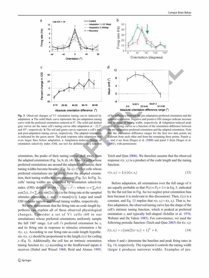
Our formulation readily explains the observed response reduc-tion for cells tuned to the adapted stimulus (Eq. 12). However,it is known that orientation adaptation produces additionalchanges to V1 orientation tuning curves (Dragoi et al. 2001;Dragoi et al. 2000; Felsen et al. 2002; Teich and Qian 2003).Some experimental data from Dragoi et al. (2000, 2001) areshown in Fig. 3. Define the two sides of a cell’s pre-adaptationtuning curve as the near and far sides according to whether theside includes the adapted orientation or not (e.g., the left andright sides of the red tuning curve in Fig. 3b are the far andnear sides, respectively, because the right side contains theadapted orientation indicated by the green arrow). Then, theadaptation-induced changes of orientation tuning curves canbe summarized as follows. (1) Responses on the near side of atuning curve decrease (Fig. 3a, b). (2) Responses on the farside of the tuning curves increase (Fig. 3a, b). (3) For cellswhose preferred orientations are around the adapted
Comput Brain Behav
FOR APPROVAL
orientation, the peaks of their tuning curves shift away fromthe adapted orientation (Fig. 3a, b, d). (4) Also for cells whosepreferred orientations are around the adapted orientation, theirtuning widths become broader (Fig. 3a–c). (5) For cells whosepreferred orientations are far away from the adapted orienta-tion, their tuning widths become narrower (Fig. 3c). In Fig. 3c,cells’ tuning widths are quantified by orientation selectivity
index (OSI) defined as OSI ¼ffiffiffiffiffiffiffiffiffiffiffiffiffiffiffiffiffiffiðα2 þ β2
q=γ where α =∑xr(x)
cos(2x), β =∑xr(x) sin(2x), r(x) is the firing rate at the sampledstimulus orientation x, and γ =mean[r(x)]. Large and smallOSI indicate narrow and broad tuning widths, respectively.
We now demonstrate that the firing-rate-as-code-length hy-pothesis can explain all of these observed physiologicalchanges . Consider a se t of V1 cel ls (60 in oursimulations) whose preferred orientations uniformly samplethe full 180° range. Let cell i’s preferred orientation be xiand its firing rate in response to stimulus orientation x ber(x, xi). According to our firing-rate-as-code-length hypothe-sis, r(x, xi) should be proportional to the length L(x) for codingx (Eq. 5). Additionally, the cell has an intrinsic orientationtuning function t(x, xi) according to the feedforward inputs itreceives (Hubel and Wiesel 1968; Reid and Alonso 1995;
Teich and Qian 2006). We therefore assume that the observedresponse r(x, xi) is a product of the code length and the tuningfunction:
r x; xið Þ ¼ L xð Þt x; xið Þ ð13Þ
Before adaptation, all orientations over the full range of πare equally probable so that P(x) = P0 = 1/π in Eq. 5, indicatedby the flat red line in Fig. 4a (we neglect prior orientation biashere because it is irrelevant to this discussion). Then, L(x) is aconstant, and Eq. 13 implies that r(x, xi) ∝ t(x, xi). That is, be-fore adaptation, the observed tuning curve has the shape of thecell’s intrinsic tuning function, which is peaked at preferredorientation xi and typically bell-shaped (Schiller et al. 1976;Webster and De Valois 1985). For convenience, we used thefollowing periodic function (Teich and Qian 2003) for t(x, xi):
t x; xið Þ ¼ c cos 2 x−xið Þ½ � þ 1f gk þ b; ð14Þ
where b and c determine the baseline and peak firing rates inEq. 14, respectively. The exponent k controls the tuning width(larger k produces narrower width). Examples of pre-
Fig. 3 Observed changes of V1 orientation tuning curves induced byadaptation. a The solid black curve represents the pre-adaptation tuningcurve with the preferred orientation centered at 0°. The solid and dashedgray curves are the same cell’s tuning curves after adaptation at − 22.5°and 45°, respectively. b The red and green curves represent a cell’s pre-and post-adaptation tuning curves, respectively. The adapted orientationis indicated by the green arrow. The peak response after adaptation waseven larger than before adaptation. c Adaptation-induced change oforientation selectivity index (OSI, see text for definition) as a function
of the difference between the pre-adaptation-preferred orientation and theadapted orientation. Negative and positive OSI changes indicate increaseand decrease of tuning width, respectively. d Adaptation-induced peakshift of tuning curves as a function of the orientation difference betweenthe pre-adaptation-preferred orientation and the adapted orientation. Notethat the orientation difference ranges for the first two data points aredifferent from each other and from the remaining three points. Panels a,c, and d are from Dragoi et al. (2000) and panel b from Dragoi et al.(2001), with permissions
Comput Brain Behav

FOR APPROVAL
adaptation tuning curves (i.e., r(x, xi) as a function of x forfixed xi) with k = 4 are shown in red in Figs. 4 and 5, panels band c.
Now assume that there is adaptation at 0° orientation, andafter adaptation, P(x) = Pa(x). Although we do not yet knowexactly how the brain updates P(x) represented by interneu-rons (see BNML and Learning^ section), Pa(x) should haveincreased values at and around the adapted orientation anddecreased values at other orientations, as we argued in con-nection with Eq. 12. We therefore used the following expres-sion:
Pa xð Þ ¼ P0 þ A zþ cos 2xð Þ þ 1½ �m−z− cos 2xð Þ þ 1½ �nf g; ð15Þwhere the two cosine terms determine the increase and de-crease of probabilities at different orientations, respectively.z+ and z− are not free parameters but normalize the two cosineterms so that Pa(x) is normalized. m and n together control theorientation ranges of the probability increase and decrease,and A determines the strength of adaptation. When n = 0, Eq.15 reduces to:
Pa xð Þ ¼ P0 þ A zþ cos 2xð Þ þ 1½ �m−P0f g; ð16Þand an example with m = 4 and A = 0.9 is shown as the greencurve in Fig. 4a. Relative to the constant baseline P0(x) (flatred line in Fig. 4a), this Pa(x) has increased values at andaround the adapted orientation and uniformly decreased
values at other orientations. When n > 0, Pa(x) has non-uniformly decreased values at the other orientations and anexample with n = 0.2,m = 4, and A = 0.9 is shown as the greencurve in Fig. 5a. This could occur if the updating of P(x)during adaptation depends on the so-called Mexican-hat con-nectivity profile among cells tuned to different orientations(Teich and Qian 2006; Teich and Qian 2010). The broad peaksof Pa(x) in Figs. 4a and 5a reflect the fact that the brain’sestimation of an individual orientation is poor (Ding et al.2017).
Plugging post-adaptation P(x) = Pa(x) into Eqs. 5 and 13,we can then determine the tuning curves that reflect theadaptation-induced change of code length. Figures 4 and 5,panels c and d, compare the pre-adaptation (red) and post-adaptation (green) tuning curves for cells whose preferredorientations are 0°, 15°, and 30° away from the adapted ori-entation at 0° (green arrow). These simulation results explainall the adaptation-induced tuning changes listed above.
Dragoi et al. (2000) measured the adaptation-induced per-cent change in OSI and shift of tuning peak (Fig. 3, panels cand d). The corresponding simulations using the two differentPa(x) in Figs. 4a and 5a are shown in Fig. 6. Results similar tothe simulations in Figs. 4, 5, and 6 can be obtained with manyother parameter sets.
We conclude that the observed tuning changes inducedby adaptation may reflect the brain’s adjustment of codelengths for different orientations after adaptation. Since at
−90 −45 0 45 900
0.01
0.02
0.03
Pro
b. d
ensi
ty (
1/de
g)Orientation (deg)
−90 −45 0 45 900
10
20
30
40
50
Firi
ng r
ate
(sp/
s)
Orientation (deg)
−90 −45 0 45 900
10
20
30
40
50
Firi
ng r
ate
(sp/
s)
Orientation (deg)−90 −45 0 45 900
10
20
30
40
50
Firi
ng r
ate
(sp/
s)
Orientation (deg)
a b
c d
Fig. 4 The firing-rate-as-code-length hypothesis explains theadaptation-induced changes oforientation tuning curves. Theadapted orientation is assumed tobe 0° indicated by the green arrowin each panel. a The orientationprobability distributions before(red) and after (green) theadaptation. b–d Comparison oftuning curves before (red) andafter (green) the adaptation forcells whose preferred orientationsare 0, 15, and 30° away from theadapted orientation, respectively
Comput Brain Behav

FOR APPROVAL
0 15 30 45 60 75 90−50
−25
0
25
50
Per
cent
cha
nge
in O
SI
0 15 30 45 60 75 90−50
−25
0
25
50
Per
cent
cha
nge
in O
SI
Abs. orientation difference (deg)
a b
c d
0 15 30 45 60 75 90−5
0
5
10
Pea
k sh
ift (
deg)
Abs. orientation difference (deg)
0 15 30 45 60 75 90−5
0
5
10
Pea
k sh
ift (
deg)
Abs. orientation difference (deg)
Fig. 6 The simulated percentchange in OSI (a, c) and peakshift (b, d) according to the firing-rate-as-code-length hypothesis.Simulations using the post-adaptation probability density inFig. 4a are shown in panels a andb, and those using the post-adaptation probability density inFig. 5a are shown in panels c andd
−90 −45 0 45 900
0.01
0.02
0.03
Pro
b. d
ensi
ty (
1/de
g)Orientation (deg)
−90 −45 0 45 900
10
20
30
40
50
Firi
ng r
ate
(sp/
s)
Orientation (deg)
−90 −45 0 45 900
10
20
30
40
50
Firi
ng r
ate
(sp/
s)
Orientation (deg)−90 −45 0 45 900
10
20
30
40
50
Firi
ng r
ate
(sp/
s)
Orientation (deg)
a b
c d
Fig. 5 The firing-rate-as-code-length hypothesis explains theadaptation-induced changes oforientation tuning curves. Thesame simulations as in Fig. 4except that a Mexican-hat-shapedpost-adaptation probabilitydensity function is used. Thepresentation format is identical tothat of Fig. 4
Comput Brain Behav

FOR APPROVAL
the circuit level, the tuning changes can be explained bymodifying recurrent connections among cells (Teich andQian 2003; Teich and Qian 2010), the recurrent connectionplasticity could be a physiological mechanism for onlinecode-length minimization.
Our firing-rate-as-code-length hypothesis calls for a re-interpretation of neuronal tuning curves. Consider, for exam-ple, V1 cells tuned to vertical orientation. The traditional viewis that when they fire, they signal the presence of verticalorientation on retina. According to theMDL framework, thesecells’ firing not only signals the presence of vertical orienta-tion. In addition, their firing rates are modulated up or downaccording to whether vertical orientation is less or more prob-able than other orientations. This interpretation is also consis-tent with the observation that natural images usually evokeweaker neural responses than isolated patches of natural im-ages or artificial stimuli (Gallant et al. 1998) because the for-mer, with its large context, is more probable than the latter.
Top-down Attention, NML with Data Prior,and Feedback Connections
In addition to the adaptation and bottom-up attentiondiscussed above, top-down attention can also be incorporatedinto the MDL framework. In the case of bottom-up attention,salient stimuli, because of their small probabilities reflected inthe NML distributions, have longer code lengths and drivecells to higher firing rates. For top-down attention, on theother hand, the brain seeks a specific type of informationbased on its current functional needs. Such information-seeking could be realized, in the MDL framework, by a top-down modulation of the NML probabilities in lower levels.For example, area V1 may normally assign horizontal orien-tation a certain probability, and the corresponding firing rate,based on actual frequencies of orientations in the input. Now ifhorizontal orientation becomes subjectively more important(e.g., when searching for a horizontal key slot), then higher-level visual areas could use top-down, feedback connectionsto V1 to reduce the estimated probability of, and thus increasethe firing rate to, horizontal orientation. In other words, sincerare stimuli are bottom-up salient, the top-down process couldinstruct lower-level areas to treat a task-relevant stimulus as ifit were rare, to boost its saliency. Thus, we must modify theMDL principle to take into account task relevance or subjec-tivity of information content, an aspect not encompassed byprevious efficient/predictive coding theories.
Zhang (2011) introduced a positive data prior function,s(x), to modify the NML distribution as:
PNML xð Þ ¼s xð ÞP xjθ̂ xð Þ
h i
∑ys yð ÞP yjθ̂ yð Þ
h i ð17Þ
This is precisely what we need for modeling top-down at-tention. The data prior function s(x) emphasizes certain inputs,at the expense of other inputs, according to the current, task-relevant need of the brain. Specifically, when a certain x is task-relevant, top-down attention will reduce its s(x), increasing thecode length (firing rate) for it. Alternatively, s(x) can be viewedas modifying the models’ likelihood functions in Eq. 17. Infact, there can be a dual relationship between data prior andmodel prior (Zhang 2011), which produce so-called informa-tive versions of MDL (Grunwald 2007).
Thus, according to theMDL framework, a major role of top-down, feedback connections in the brain, is for higher levels tomodify the lower-level model classes in order to increase trans-mission of behaviorally relevant information. The framework isconsistent with the fact that top-down attention is slower thanbottom-up attention because it takes time for high-level areas tosend spikes down the feedback connections to modify NMLdistributions of lower-levels. This is fundamentally differentfrom Rao and Ballard’s proposal that feedback connectionssend higher-level predictions of inputs to the lower level forsubtraction (Rao and Ballard 1999). The difference reflects dif-ferent aims of the two approaches. Rao and Ballard’s model, asare typical of most efficient/predictive coding models, aims toreconstruct retinal inputs. Therefore, a high-level sends its inputprediction to the lower level, which subtracts this prediction andsends the error to the higher level for improvement. In contrast,our MDL framework focuses on regularity extraction to servethe brain’s needs of sensory processing without input recon-struction. Although regularity extraction is the basis for bothefficient coding and prediction, in theMDL framework, there isno input prediction coming from higher levels for lower-levelsto subtract. Instead, NML unifies prediction, regularity extrac-tion, and efficient coding at each level of processing.
Top-down processes may also direct motor outputs (includ-ing eye movements) to actively seek relevant information inthe world.
Comparison with Existing Models
Our firing-rate-as-code-length hypothesis differs significantlyfrom previous theories. We already mentioned some differ-ences above. Here, we recapitulate the discussions and makesome further comparisons. Although negative log probabilityis frequently used in the literature for computational conve-nience or for linkage to MDL concepts, to our knowledge, thefiring-rate-as-code-length hypothesis for interpreting sensoryneurons’ responses has not been proposed.
Predictive Coding Models
Rao and Ballard (1999) used a two-part version of MDL(Rissanen 1978; Rissanen 1983) in their predictive coding
Comput Brain Behav

FOR APPROVAL
model, which, like other efficient/predictive coding models,aims to reconstruct the retinal image. Our NML-based MDLframework is very different in that it uses regularity extractionto serve the brain’s functional needs rather than to reconstructretinal images, and consequently, interprets neuronal re-sponses and connections differently. In particular, Rao andBallard’s model and our framework interpret projection neu-rons’ responses as representing errors of input reconstructionand coding useful features in the input, respectively.Additionally, while they assume that feedback connectionscarry the higher-level’s prediction of the lower-level input,we assume that feedback connections modify the lower-level’s model classes to transmit task-relevant information inthe input.
Firing-Rate-As-Probability Theories
Firing-rate-as-probability theories, including a proposed im-plementation of Bayesian inference (Ma et al. 2006), posit thatprojection neurons transmit probability distributions of inputfeatures (or parameterizations of the distributions), whereaswe suggest that the probability distributions computed in anarea are not transmitted but are used to code input featuresefficiently and that probability distributions computed in dif-ferent areas are relative to different model classes and concerndifferent regularities of the inputs. As we noted in theBEvaluations of Major Theories of Neuronal Coding^ section,firing-rate-as-probability theories are not consistent with ad-aptation and bottom-up-attention phenomena while ourframework is. Note that we are not arguing against Bayesianinference, only the firing-rate-as-probability assumption usedin many models including those that have been calledBayesian inference models. In fact, the Bayesian universalcode with Jeffery’s prior asymptotically achieves the minimaxoptimal regret of the NML code and may well be used by thebrain because of its prequential property which is useful forprediction without a pre-specified time horizon (Grunwald2007).
Saliency Models
Zhaoping (2002) proposed that V1 constructs a bottom-upsaliency map such that, for a given visual scene, firing rateof V1 output neurons increases monotonically with the salien-cy values of the visual input in the classical receptive fields.There are no separate feature maps for creating such a bottom-up saliency map. Neuronal responses encode universal valuesof saliency that govern subsequent actions (e.g., saccades). Inour framework, neuronal responses are also related to salien-cy. However, this is realized via neurons’ firing rates beingproportional to the code lengths for coding useful features.The code lengths are determined by the features’ probabilities,which, in turn, are related to the saliency values.
Han and Vasconcelos (2010) presented another saliencymodel for object recognition in biological systems.Motivated by the observation that stimulus features with highbottom-up saliency have a low probability of occurrence, theyproposed a top-down saliency measure using log likelihoodratio of Gabor-filter responses to target and non-target objectsand demonstrated that this computation can be realized by aselective normalization procedure. In contrast, we assume thatthe top-down attention modifies lower-level NML distribu-tions for coding-relevant stimulus features. More importantly,they eventually let cells’ firing rates represent the posteriorprobability of target object via a nonlinear function of thelog likelihood ratio so their model follows the traditionalfiring-rate-as-probability assumption. Instead, we assume thatfiring rates represent code length, not probability.
Normalization Models
On first glance, the NML distribution (Eq. 8) resembles thenormalization models for sensory responses (Eq. 4), and theNML distribution with a data prior (Eq. 17) resembles thenormalization models for attentional modulation (Reynoldsand Heeger 2009). However, the normalization factors(denominators) in NML and in normalization models are verydifferent. In NML, the denominator sums the maximum like-lihood of a model class across all input data samples. In nor-malization models, the denominator is a constant plus thesummed responses of all cells with a range of tuning (i.e., allcells in a model class) to the current input sample.
A key motivation for the normalization models is to fit V1cells’ contrast response curves. Indeed, the form of the nor-malization models mimics contrast saturation functions. TheMDL framework offers an alternative, computational-levelexplanation of contrast responses, namely that high contrastoccurs less frequently than low contrast in the real world; thisreflects the fact that the world consists of coherent surfaces ofobjects and high contrast typically occurs at relatively rareobject boundaries whereas low contrast typically occurs atrelatively abundant object interiors. Indeed, Ruderman(1994) measured contrast distribution of natural images andhis result can be approximated by:
P cð Þ ¼ a−blog 1þ cð Þ ð18Þwhere c is the contrast and a and b are the positive constants;the probability decreases with contrast. If, as we postulatedearlier, the brain learns this statistical regularity based on theMDL principle, then the corresponding NML distribution forencoding stimulus contrast should reflect the statistics. Thecontrast responses of projection neurons covering differentranges of contrast should then have the envelope -log P(c), acurve resembling saturation. Thus, contrast response may notresult from shunting inhibition of pooled responses to a given
Comput Brain Behav

FOR APPROVAL
stimulus; rather, it may reflect code-length optimization by acircuit that sample contrast statistics from many stimuli.
The MDL framework may also account for phenomenathat the normalization models fail to explain. For example,we mentioned above that end-stopped V1 cells fire less whena contour extends beyond their classical receptive fields (Bolzand Gilbert 1986; Hubel and Wiesel 1968). More generally,V1 or MT cells’ responses to their preferred orientation/direction within the classical receptive fields are suppressedwhen the surround has the same orientation/direction, but thesuppression becomes weaker, or even turns into facilitation,when the surround orientation/direction differs greatly(Allman et al. 1985; Levitt and Lund 1997; Nelson andFrost 1978). The normalization models cannot explain theseresults because the normalization factor is untuned. Of course,one could modify the normalization models by making thenormalization factor follow the observed results; however, thismeans that the normalization models have to be adjusted foreach specific situation. The MDL framework may be able toexplain these experimental findings because when the classi-cal receptive field and its surround have similar (different)stimuli, the presence of the surround stimuli increases(decreases) the probability of the stimuli in the classical recep-tive field, and consequently, a shorter (longer) code length, inthe form of a lower (higher) firing rate, is needed to transmitthe information. Similarly, when a contour extends smoothlybeyond an end-stopped cell’s classical receptive field, theprobability of the segment inside the receptive field is in-creased, leading to a shorter code length (reduced firing) ofthe cell.
Lossy MDL and Prefix-Free Neural Code
The standard MDL uses the terms Bcode^ and Bprobabilitydistribution^ interchangeably because once a probability dis-tribution is specified, one can always design a lossless, prefix-free code (a.k.a., prefix code) that saturates the Kraft–McMillan inequality such that the code length is equal tonegative log probability (Grunwald 2007). In contrast, phe-nomena such as change blindness (Pashler 1988) suggest thatthe brain uses a lossy code to transmit behaviorally relevantinformation and discard irrelevant details of the input. We willtherefore speculate on a lossy MDL code as a candidate forneural code. To motivate our proposal, consider the exampleof seeing something moving in a jungle. The most survival-relevant information may be whether the moving thing is apredator or a pray. If it is a predator, the next most relevantinformation may be whether it is the type that one could fightagainst (e.g., a wolf) or better flee from (e.g., a tiger). Tooptimize survival, the brain should use its visual neurons’ firstfew spikes to transmit the most relevant information, and thenext few spikes to transmit the second most relevant informa-tion, and so on. Only crude aspects of low-level features that
are sufficient for building relevant, high-level categorical de-cisions should be transmitted quickly. It would be a hugemistake to waste the precious first several spikes on transmit-ting, for example, the precise orientation of a stripe on theanimal’s fur. On the other hand, the brain is certainly able tojudge the orientation when one is asked to do so in a safesetting.
These considerations suggest that a partially transmittedcode should be meaningful so that a brain area can start pro-cessing inputs immediately after receiving spikes from lowerareas, that the code should be as short (efficient) as possibleand carry pieces of information ordered according to theirbehavioral relevance/urgency, and that higher-level areasshould instruct lower-level areas on what and how much de-tails to transmit depending on the situation. Therefore, thebrain might use entropic, prefix-free codes (based on NMLdistributions) with earlier spikes carrying more behaviorallyimportant information.
Consider the toy example in Table 1 of coding four sym-bols (column 1) with known probabilities (column 2). Code 1is fixed length and inefficient (the length of 2 bits/symbol isgreater than the entropy of 1.75 bits/symbol). Code 2 is theHuffman code, which is entropic (average length 1.75bits/symbol) and prefix free (no code word is a prefix of an-other code word). Code 3 reverses the bit order of each codeword of code 2. It is entropic but not prefix free. Althoughcode 3, like the other two codes, is uniquely decodable (afterreceiving a whole message, the bit string can be reversed anddecoded according to code 2), a partial message is meaning-less. In contrast, a Huffman-coded string can be decoded on-line as each bit is received without the need to wait for a wholemessage or a whole code word. For example, the first bitdivides choices into A vs. (B, C, D). Because each bit of acode word divides the remaining choices into two sets withequal probabilities, the bits are ordered from the most to leastinformative. (Although the Huffman code is a symbol code,similar arguments could be made with the entropic, arithmeticcoding for blocks of arbitrary lengths.)
We propose that the brain might use a Huffman-like code(or arithmetic-like coding) based on NML distributions. Sucha code is attractive because of the efficiency, the bit orderingfrom themost to least informative, and the prefix-free property
Table 1 Three codes for the four symbols with the given probabilities.Codes 1 and 2 are prefix free. Codes 2 and 3 are entropic. Code 2(Huffman) is both prefix free and entropic
Symbol Probability Code 1 Code 2 Code 3
A 1/2 00 0 0
B 1/4 01 10 01
C 1/8 10 110 011
D 1/8 11 111 111
Comput Brain Behav

FOR APPROVAL
allowing immediate decoding as each bit comes in. We sug-gest that neural codes should be similar in that the first spikesof a neuronal population carry the most task/situation-relevantinformation so that the brain can take most pressing actions atthe earliest possible time. The later spikes carry less relevantdetails that may be truncated by top-down instructions or by achange of inputs (e.g., a saccade to a different part of the worldor a changing world), resulting in a lossy code. Experimentsthat present stimuli for only several to tens of millisecondsprovide indirect evidence for the prefix-free and lossy natureof neural codes: subjects could identify global or high-level,categorical features better than local or low-level details (Chen1982; Navon 1977; Thorpe et al. 1996), suggesting that trun-cated visual transmission is meaningful and that the transmis-sion leading to high-level categorization, which is more be-haviorally relevant than low-level details, is prioritized.
In information theory, the rate-distortion curve is a standardtool for studying lossy transmission (Blahut 1972). Each pointof the curve specifies the minimum input information that hasto be transmitted to the output (i.e., the rate) in order to keepthe average distortion under a given value. Equivalently, eachpoint specifies the minimum average distortion for a givenrate. The distortion for each input/output pair is pre-defined.(The rate is similar to channel capacity except that the formeris the mutual information minimized against the channel tran-sition probabilities whereas the latter is the mutual informationmaximized against input distribution. We will not distinguishthe two terms in the following for simplicity.) The rate-distortion curve has been used as a computational-level theoryfor understanding discrimination vs. generalization in percep-tion (Sims 2018). The main idea is that when a system trans-mits inputs whose information (i.e., entropy) exceeds the sys-tem’s channel capacity, the output will have distortion whichdetermines discrimination between, or generalization across,different inputs. The information bottleneck theory (Tishbyet al. 2000) is a version of the rate-distortion theory in whichthe distortion for each input/output pair is not pre-defined, butdetermined according to how much information the outputcarries about the input’s assigned label (e.g., the label Bcat^for an input image). The truncated, lossy code discussedabove could be viewed as a possible neural implementationof the rate-distortion function. Specifically, because of thelimited rate or channel capacity, projection neurons cannottransmit all input information as stimuli stream in, and trun-cated transmission leads to distortion. If the spikes of a neuralcode are arranged from the most to least relevance to currentbehavior, then the distortion with respect to the behaviorBlabel^ is minimized for a given rate of transmission.
The firing-rate-as-code-length hypothesis implies that thechannel capacity (firing rates) of projection neurons is dynam-ic, being greater for lower-probability stimuli which requirelonger codes. This ensures that unexpected, salient stimuli arenot truncated more than common stimuli.
Encoding Vs. Decoding
Coding can be divided into encoding and decoding. The engi-neering notion of encoding and decoding is well defined:When a signal needs to be transmitted over a noisy communi-cation channel of limited capacity (e.g., a phone line), oneshould encode the signal to compress it (while allowing errorcorrection), transmit it, and then decode it to recover the orig-inal signal on the other end. It is widely assumed that the braindoes similar encoding and decoding. Our MDL frameworksuggests that the brain encodes input stimuli into neuronalresponses but does not decode the responses to recover theoriginal inputs. The main reason is that, unlike a phone linethat has to reproduce the input voice at the other end, the brainnever needs to reconstruct the raw sensory inputs it receives.Rather, as we already emphasized, the brain attempts to under-stand the sensory inputs by processing them. For example, thebrain processes the retinal images to reveal objects and theirrelationships but hardly needs to reconstruct the retinal imagesbecause retina is part of the brain and no homunculus exists inthe cortex to look at the reconstructed images. More generally,it is hard to imagine that one brain area needs to accuratelyreconstruct neural firing patterns (spike trains) of another area;rather, a brain area should extract additional regularity from,and thus achieve further understanding of, the input. If thefiring patterns of a sensory area are needed, for instance, toguide a certain motor response, then themotor area of the brainshould use the firing patterns directly, instead of encoding,transmitting, and decoding. For example, in the unlikely sce-nario that raw retinal image was needed, the brain would haveevolved to use the retinal image instead of decoding a poorerversion of it from, say, LGN or V1 responses.
One may reasonably identify the brain’s logic of relatingneuronal responses to subjective perception as decoding.Note, however, that this decoding is fundamentally differentfrom the engineering notion of decoding. Specifically, neuro-nal responses along hierarchical stages of sensory pathwaysextract and encode progressively more complex statistical reg-ularities in the input stimuli. A small subset of these responsespresumably gives rise to our subjective perception of usefulfeatures in inputs without any need of reconstructing the rawinputs. We therefore suggest that neural decoding should beviewed as the link from neuronal responses to perceptual es-timation of useful stimulus features, but not as input recon-struction. Also, note that encoding and decoding are oftenrelated; for example, the population-average method of Eq.1 is a decoding model but it implies that firing rates encodethe probabilities of preferred stimuli.
A related question is whether sensory decoding follows thesame low-to-high-level hierarchy of sensory encoding. Manystudies assume, often implicitly, that the answer is affirmative.However, a recent study shows that this assumption fails toexplain a simple psychophysical experiment and suggests that
Comput Brain Behav

FOR APPROVAL
visual decoding progresses from high-to-low-level features inworking memory, with higher-level features constraining thedecoding of lower-level features (Ding et al. 2017). Sincehigher-level features have greater functional significance thanlower-level features, this decoding scheme is consistent withthe above notion that the brain should prioritize transmissionof behaviorally relevant information.
NML and Learning
Given the importance of the NML distribution (or a relatedOUC as its approximation) in the MDL framework, a relevantquestion is how can a brain area produce such a distributionparticularly when the input data space is high dimensional?Variational methods in machine learning provide a potentialanswer as they have demonstrated that neural networks canlearn complex probability distributions via gradient decent(Dayan et al. 1995; Kingma andWelling 2013) or even a localplasticity rule (Hinton et al. 1995). To outline the approach forthe NML distribution (Eq. 8), we define the Benergy^ of a datasample x relative to a model class parameterized by θ as:
E xð Þ ¼ −logP xjθ̂ xð Þh i
ð19Þ
(i.e., the code length according to the model in the class thatmaximizes the likelihood of the sample) and rewrite Eq. 8 inthe form of a Boltzmann distribution (with β = 1):
PNML xð Þ ¼ exp −E xð Þ½ �∑yexp −E yð Þ½ � ð20Þ
The numerator is known as the partition functionZ≡∑
yexp −E yð Þ½ �, and the regret and complexity measure in
Eqs. 9 and 10 become logZ. Use the standard definition ofHelmholtz free energy as the mean energy minus entropy:
A ¼ ∑xP xð ÞE xð Þ þ ∑
xP xð ÞlogP xð Þ ð21Þ
for any probability distributionP(x). Then (Dayan et al. 1995),
A ¼ −logZ þ KL P xð Þ‖PNML xð Þh i
ð22Þ
where KL is the Kullback–Leibler divergence. Since KL isnon-negative and minimized to 0 when the two distributionsare equal, A reaches the minimum value of − log Z whenP(x) = PNML(x). (The physical analogy is that Helmholtz freeenergy A approaches the minimum − log Z when any non-equilibrium distribution P(x) approaches the equilibrium,Boltzmann distribution PNML(x).) Therefore, if P(x; ϕ) is afamily of probability distributions parameterized by weightsϕ of a neural network, then the network could be trained toapproximate PNML(x) by minimizing the cost A in Eq. 21
against ϕ as input data are sampled, and –A is a lower boundfor log Z (Dayan et al. 1995; Friston 2010; Hinton et al. 1995;Kingma and Welling 2013). If data statistics are changed, theneural network’s approximation of PNML(x) would changeaccordingly (as we assumed in the example of orientationadaptation in BSimulating Adaptation-Induced Changes ofV1 Orientation Tuning Curves^ section).
Moreover, E(x) and log Z depend on the model-class pa-rameterization θ, which can also be implemented as weights ofa neural network. One could thus, for example, adjust theequilibrium Helmholtz free energy (A = − log Z) by modify-ing θ in order to control the NML regret or complexity (logZ).Since the model-class complexity and the code length for aninput (i.e., neuronal firing rate) may be related to coding spar-sity, this could be a mechanism for adjusting the degree ofsparsity. Finally, the learning of the ϕ and θ parameters couldbe interleaved.
Discussion
Understanding the nature of neural code is of fundamentalimportance. Although extant theories have been successfulin revealing many properties of neural coding, they are notalways consistent with major empirical observations or witheach other. Our efforts in this project focus on proposing anovel, modernMDL-based framework for characterizing neu-ral code. The framework aims to integrate the strengths ofextant theories, explain (or at least be consistent with) moreempirical observations, and unify sensory processing and at-tention. The framework leads to the specific proposal thatneural firing rates are proportional to code lengths given bynegative log NML probability distributions (or closely relatedOUCs) for stimulus features. We showed via simulations thatthis firing-rate-as-code-length hypothesis can explain all theobserved changes of V1 orientation tuning curves induced byorientation adaptation.
Our framework contains five essential elements, the com-bination of which, to our knowledge, has never been sug-gested before.
1. The firing rates of sensory projection neurons are propor-tional to code length, not the probability or its parameter-ization, of stimulus features. Indeed, for efficient trans-mission of inputs, a system should use a proper probabil-ity distribution to encode/compress the inputs instead oftransmitting the probability distribution itself.
2. The code length is based on an OUC (such as NML dis-tribution) of a given model class which maximizes regu-larity extraction, predictive ability, and data compressionto achieve input understanding by balancing data fittingand model-class complexity. Parameters specifying a
Comput Brain Behav

FOR APPROVAL
model class and its NML distribution might be learned ortuned together.
3. The actual code in the temporal firing pattern of a neuro-nal population is Huffman-like such that it has minimalfiring rates, is prefix free, and the order of informationtransmission is from the most relevant to the least relevantaccording to the current task or goal. In this way, a par-tially transmitted message is meaningful and can be proc-essed immediately by the next stage, the system couldrespond to the most relevant aspect of input with theshortest delay, and a truncated, lossy transmission wouldminimize behaviorally relevant distortion.
4. The brain does not really face a decoding problem in theform of input reconstruction because the input represen-tation is already in the brain. Rather, the brain extractsuseful stimulus features during efficient encoding, with-out the need to reconstruct the original input signal. Thebrain processes input hierarchically to extract progressive-ly more complex and global regularities to serve variousperceptual and motor functions.
5. Top-down signals are sent to modulate lower-level modelclasses, direct eyes to relevant regions, and set prior ex-pectations of data statistics, to allow selective processingof informative and relevant inputs according to the currenttask demand.
Needless to say, any theory is only a crude approximationof reality but we hope our MDL framework will provide afresh perspective for characterizing neural code. Future em-pirical data may be able to evaluate our specific, firing-rate-as-code-length hypothesis and our speculations on the nature ofneural codes in sensory firing patterns.
Acknowledgments We thank Dr. Jay Myung for encouraging us to ex-plore this topic and for his many helpful comments and suggestions.
Funding Information This work was supported by AFOSR FA9550-15-1-0439 and NSF 1754211.
Publisher’s Note Springer Nature remains neutral with regard to juris-dictional claims in published maps and institutional affiliations.
References
Adrian, E. D. (1926). The impulses produced by sensory nerve endings.The Journal of Physiology, 61, 49–72.
Albrecht, D. G., & Geisler, W. S. (1991). Motion selectivity and thecontrast-response function of simple cells in the visual cortex.Visual Neuroscience, 7, 531–546.
Allman, J., Miezin, F., & McGuinness, E. (1985). Stimulus specific re-sponses from beyond the classical receptive field: neurophysiologi-cal mechanisms for local-global comparisons in visual neurons.Annual Review of Neuroscience, 8, 407–430.
Anderson, J. S., Carandini, M., & Ferster, D. (2000). Orientation tuningof input conductance, excitation, and inhibition in cat primary visualcortex. Journal of Neurophysiology, 84, 909–926.
Atick, J. J., & Redlich, A. N. (1990). Towards a theory of early visualprocessing. Neural Computation, 2, 308–320.
Balasubramanian, V., Berry, M. J., & Kimber, D. (2001). Metabolicallyefficient information processing.Neural Computation, 13, 799–816.
Barlow, H. (1972). Single units and sensation: a neuron doctrine forperceptual psychology? Perception, 1(4), 371–394.
Barlow, H., & Foldiak, P. (1989). Adaptation and decorrelation in thecortex. In R. Durbin, C. Miall, & G. Mitchinson (Eds.), The com-puting neuron (pp. 54–72). New York: Addison-Wesley.
Barron, A., Rissanen, J., & Yu, B. (1998). The minimum descriptionlength principle in coding and modeling. IEEE Transactions onInformation Theory, 44, 2743–2760.
Bell, A. J., & Sejnowski, T. J. (1997). The Bindependent components^ ofnatural scenes are edge filters. Vision Research, 37, 3327–3338.
Blahut, R. E. (1972). Computation of channel capacity and rate-distortionfunctions. IEEE Transactions on Information Theory, 18, 460–473.
Blakemore, C., & Campbell, F. W. (1969). Adaptation to spatial stimuli.The Journal of Physiology, 200, 11P–13P.
Bolz, J., & Gilbert, C. D. (1986). Generation of end-inhibition in thevisual cortex via interlaminar connections. Nature, 320, 362–365.
Carandini, M., & Heeger, D. J. (2012). Normalization as a canonicalneural computation. Nature Reviews. Neuroscience, 13, 51–62.
Carandini, M., Heeger, D. J., & Movshon, J. A. (1997). Linearity andnormalization in simple cells of the macaque primary visual cortex.The Journal of Neuroscience, 17, 8621–8644.
Chen, L. (1982). Topological structure in visual perception. Science, 218,699–700.
Dayan, P., Hinton, G. E., Neal, R. M., & Zemel, R. S. (1995). TheHelmholtz machine. Neural Computation, 7, 889–904.
Ding, S., Cueva, C. J., Tsodyks, M., & Qian, N. (2017). Visual perceptionas retrospective Bayesian decoding from high- to low-level features.Proceedings of the National Academy of Sciences, 114, E9115–E9124.
Dragoi, V., Sharma, J., & Sur, M. (2000). Adaptation-induced plasticityof orientation tuning in adult visual cortex. Neuron, 28, 287–298.
Dragoi, V., Rivadulla, C., & Sur, M. (2001). Foci of orientation plasticityin visual cortex. Nature, 411, 80–86.
Fang, F., Murray, S. O., Kersten, D., & He, S. (2005). Orientation-tunedfMRI adaptation in human visual cortex. Journal of Neurophysiology,94, 4188–4195.
Felsen, G., Shen, Y. S., Yao, H., Spor, G., Li, C., & Dan, Y. (2002).Dynamic modification of cortical orientation tuning mediated byrecurrent connections. Neuron, 36, 945–954.
Field, D. J. (1987). Relations between the statistics of natural images andthe response properties of cortical-cells. Journal of the OpticalSociety of America. A, Optics, Image Science, and Vision, 4,2379–2394.
Flash, T., & Hogan, N. (1985). The coordination of arm movements - anexperimentally confirmed mathematical-model. The Journal ofNeuroscience, 5, 1688–1703.
Friston (2010). The free-energy principle: a unified brain theory? NatureReviews Neuroscience, 11, 127–138.
Gallant, J. L., Connor, C. E., & Van Essen, D. C. (1998). Neural activityin areas V1, V2 and V4 during free viewing of natural scenes com-pared to controlled viewing. Neuroreport, 9, 2153–2158.
Ganmor, E., Segev, R., & Schneidman, E. (2011). The architecture offunctional interaction networks in the retina. The Journal ofNeuroscience, 31, 3044–3054.
Geisler,W. S., Perry, J. S., Super, B. J., & Gallogly, D. P. (2001). Edge co-occurrence in natural images predicts contour grouping perfor-mance. Vision Research, 41, 711–724.
Comput Brain Behav

FOR APPROVAL
Georgopoulos, A. P., Schwartz, A. B., & Kettner, R. E. (1986). Neuronalpopulation coding of movement direction. Science, 233, 1416–1419.
Gibson, J. J., & Radner, M. (1937). Adaptation, after-effect and contrastin the perception of tilted lines. I. Quantitative studies. Journal ofExperimental Psychology, 20, 453–467.
Gottlieb, J. P., Kusunoki, M., & Goldberg, M. E. (1998). The represen-tation of visual salience in monkey parietal cortex. Nature, 391,481–484.
Grunwald, P. D. (2007). The minimum description length principle.Cambridge: MIT Press.
Grunwald, P. D., Myung, I. J., & Pitt, M. A. (2005). Advances in mini-mum description length: theory and applications. Cambridge: MITPress.
Han, S., & Vasconcelos, N. (2010). Biologically plausible saliency mech-anisms improve feedforward object recognition. Vision Research,50, 2295–2307.
Harpur, G. F., & Prager, R. W. (1996). Development of low entropycoding in a recurrent network*. Network: Computation in NeuralSystems, 7, 277–284.
Heeger, D. J. (1992). Normalization of cell responses in cat striate cortex.Visual Neuroscience, 9, 181–197.
Hinton, G., Dayan, P., Frey, B., & Neal, R. (1995). The Bwake-sleep^algorithm for unsupervised neural networks. Science, 268, 1158–1161.
Hubel, D. H., & Wiesel, T. N. (1968). Receptive fields and functionalarchitecture of monkey striate cortex. The Journal of Physiology,195, 215–243.
Itti, L., & Koch, C. (2001). Computational modelling of visual attention.Nature Reviews. Neuroscience, 2, 194–203.
Khaligh-Razavi, S.-M., & Kriegeskorte, N. (2014). Deep supervised, butnot unsupervised, models may explain IT cortical representation.PLoS Computational Biology, 10, e1003915.
Kingma DP, Welling M. (2013). Auto-encodrwing variational bayes.arXiv preprint arXiv:1312.6114.
Levitt, J. B., & Lund, J. S. (1997). Contrast dependence of contextualeffects in primate visual cortex. Nature, 387, 73–76.
Li, W., & Gilbert, C. D. (2002). Global contour saliency and local colin-ear interactions. Journal of Neurophysiology, 88, 2846–2856.
Li, C.-Y., & Li, W. (1994). Extenstive integration field beyond the clas-sical receptive field of cat’s striate cortical neurons - classificationand tuning properties. Vision Research, 34, 2337–2355.
Ma, W. J., Beck, J. M., Latham, P. E., & Pouget, A. (2006). Bayesianinference with probabilistic population codes. Nature Neuroscience,9, 1432–1438.
Meng, X., & Qian, N. (2005). The oblique effect depends on perceived,rather than physical, orientation and direction. Vision Research, 45,3402–3413.
Motoyoshi, I., Sy, N., Sharan, L., & Adelson, E. H. (2007). Image statis-tics and the perception of surface qualities. Nature, 447, 206–209.
Myung, J. I., Navarro, D. J., & Pitt, M. A. (2006). Model selection bynormalized maximum likelihood. Journal of MathematicalPsychology, 50, 167–179.
Navon, D. (1977). Forest before trees: the precedence of global features invisual perception. Cognitive Psychology, 9, 353–383.
Nelson, J. I., & Frost, B. J. (1978). Orientation-selective inhibition frombeyond the classic visual receptive field. Brain Research, 139, 359–365.
Nowak, L. G., Munk, M. H., Nelson, J. I., James, A. C., & Bullier, J.(1995). Structural basis of cortical synchronization. I. Three types ofinterhemispheric coupling. Journal of Neurophysiology, 74, 2379–2400.
Olshausen, B. A., & Field, D. J. (1996). Emergence of simple-cell recep-tive field properties by learning a sparse code for natural images.Nature, 381, 607–609.
Olshausen, B. A., & Field, D. J. (2004). Sparse coding of sensory inputs.Current Opinion in Neurobiology, 14, 481–487.
Paradiso, M. A. (1988). A theory for the use of visual orientation infor-mation which exploits the columnar structure of striate cortex.Biological Cybernetics, 58, 35–49.
Pashler, H. (1988). Familiarity and visual change detection. Attention,Perception, & Psychophysics, 44, 369–378.
Poggio, T., Torre, V., & Koch, C. (1985). Computational vision andregularization theory. Nature, 317, 314–319.
Qian, N. (1994). Computing stereo disparity and motion with knownbinocular cell properties. Neural Computation, 6, 390–404.
Qian, N. (1997). Binocular disparity and the perception of depth.Neuron,18, 359–368.
Rao, R. P. N., & Ballard, D. H. (1997). Dynamic model of visual recog-nition predicts neural response properties in the visual cortex.Neural Computation, 9, 721–763.
Rao, R. P. N., & Ballard, D. H. (1999). Predictive coding in the visualcortex: a functional interpretation of some extra-classical receptive-field effects. Nature Neuroscience, 2, 79–87.
Reid, R. C., & Alonso, J. M. (1995). Specificity of monosynaptic con-nections from thalamus to visual cortex. Nature, 378, 281–284.
Reynolds, J. H., & Heeger, D. J. (2009). The normalization model ofattention. Neuron, 61, 168–185.
Rissanen, J. (1978). Modeling by the shortest data description. Automata,14, 465–471.
Rissanen, J. (1983). A universal prior for integers and estimation byminimum description length. Annals of Statistics, 11, 416–431.
Rissanen, J. (1996). Fisher information and stochastic complexity. IEEETransactions on Information Theory, 42, 40–47.
Rissanen, J. (2001). Strong optimality of the normalized ML models asuniversal codes and information in data. IEEE Information Theory,47, 1712–1717.
Ruderman, D. L. (1994). The statistics of natural images. Network:Computation in Neural Systems, 5, 517–548.
Sanger, T. D. (1996). Probability density estimation for the interpretationof neural population codes. Journal of Neurophysiology, 76, 2790–2793.
Schiller, P. H., Finlay, B. L., & Volman, S. F. (1976). Quantitative studiesof single-cell properties in monkey striate cortex. II. Orientationspecificity and ocular dominance. Journal of Neurophysiology,39(6), 1320–1333.
Schneidman, E., Berry, M. J., Segev, R., & Bialek, W. (2006). Weakpairwise correlations imply strongly correlated network states in aneural population. Nature, 440, 1007–1012.
Shannon, C. E. (1948). A mathematical theory of communication. BellSystem Technical Journal, 27, 379–423.
Shlens, J., Field, G. D., Gauthier, J. L., Grivich, M. I., Petrusca, D., Sher,A., Litke, A. M., & Chichilnisky, E. J. (2006). The structure ofmulti-neuron firing patterns in primate retina. The Journal ofNeuroscience, 26, 8254–8266.
Sigman, M., Cecchi, G. A., Gilbert, C. D., & Magnasco, M. O. (2001).On a common circle: natural scenes and gestalt rules. Proceedings ofthe National Academy of Sciences of the United States of America,98, 1935–1940.
Simoncelli, E. P., & Heeger, D. J. (1998). A model of neuronal responsesin visual area MT. Vision Research, 38, 743–761.
Simoncelli, E. P., & Olshausen, B. A. (2001). Natural image statistics andneural representation. Annual Review of Neuroscience, 24, 1193–1216.
Sims, C. R. (2018). Efficient coding explains the universal law of gener-alization in human perception. Science, 360, 652–656.
Stocker, A. A., & Simoncelli, E. P. (2006). Sensory adaptation within aBayesian framework for perception. In Y. Weiss, B. Scholkopf, & J.Platt (Eds.), Advances in neural information processing systems.Cambridge: MIT Press.
Comput Brain Behav

FOR APPROVAL
Tanaka, H., Krakauer, J. W., & Qian, N. (2006). An optimization principlefor determining movement duration. Journal of Neurophysiology, 95,3875–3886.
Teich, A. F., & Qian, N. (2003). Learning and adaptation in a recurrentmodel of V1 orientation selectivity. Journal of Neurophysiology, 89,2086–2100.
Teich, A. F., & Qian, N. (2006). Comparison among some models oforientation selectivity. Journal of Neurophysiology, 96, 404–419.
Teich, A. F., & Qian, N. (2010). V1 orientation plasticity is explained bybroadly tuned feedforward inputs and intracortical sharpening.Visual Neuroscience, 27, 57–73.
Thorpe, S., Fize, D., & Marlot, C. (1996). Speed of processing in thehuman visual system. Nature, 381, 520–522.
Tishby N, Pereira FC, Bialek W. (2000). The information bottleneckmethod. arXiv:physics/0004057.
van Kan, P. L. E., Scobey, R. P., & Gabor, A. J. (1985). Response covari-ance in cat visual cortex. Experimental Brain Research, 60, 559–563.
Webster, M. A., & De Valois, R. L. (1985). Relationship between spatial-frequency and orientation tuning of striate-cortex cells. Journal ofthe Optical Society of America A. Optics and Image Science, 2,1124–1132.
Weiss, Y., Simoncelli, E. P., & Adelson, E. H. (2002). Motion illusions asoptimal percepts. Nature Neuroscience, 5, 598–604.
Yamins, D. L. K., Hong, H., Cadieu, C. F., Solomon, E. A., Seibert, D., &DiCarlo, J. J. (2014). Performance-optimized hierarchical modelspredict neural responses in higher visual cortex. Proceedings of theNational Academy of Sciences, 111, 8619–8624.
Yang, Z., & Purves, D. (2003). A statistical explanation of visual space.Nature Neuroscience, 6, 632–640.
Yenduri PK, Zhang J, Gilbert A. (2012) Proceedings of the ThirdInternational Conference on Intelligent Control and InformationProcessing, ICICIP 20122012.
Yuille, A., & Kersten, D. (2006). Vision as Bayesian inference: analysisby synthesis? Trends in Cognitive Sciences, 10, 301–308.
Zhang, J. (2011). Model selection with informative normalized maximallikelihood: data prior andmodel prior. In E. N. Dzhafarov&L. Perry(Eds.), Descriptive and normative approaches to human behavior(pp. 303–319). Hackensack: World Scientific.
Zhaoping, L. (2002). A saliency map in primary visual cortex. Trends inCognitive Sciences, 6, 9–16.
Zhaoping, L. (2014). Understanding vision: theory, models, and data.London: Oxford University Press.
Comput Brain Behav