1

New Directions in Measurement for Software Quality Control

Paul Krause, Bernd Freimut and Witold Suryn

Abstract—Assessing and controlling software quality is still an

immature discipline. One of the reasons for this is that many of the concepts and terms that are used in discussing and describing quality are overloaded with a history from manufacturing quality. We argue in this paper that a quite distinct approach is needed to software quality control as compared with manufacturing quality control. In particular, the emphasis in software quality control is in design to fulfil business needs, rather than replication to agreed standards. We will describe how quality goals can be derived from business needs. Following that, we will introduce an approach to quality control that uses rich causal models, which can take into, account human as well as technological influences. A significant concern of developing such models is the limited sample sizes that are available for eliciting their parameters. In the final section of the paper we will show how expert judgement can be reliably used to elicit parameters in the absence of statistical data. In total this provides a framework for quality control in software engineering that is freed from the shackles of an inappropriate legacy.

Index Terms—System Reliability, Quality Control, Failure Analysis, Process Control

I. INTRODUCTION SSESSING and controlling software quality is hard. You cannot hold it or touch it, yet its behaviour has an impact

on all of our lives. We all are stakeholders in the drive to improve the quality of the software that we work with, yet few of us are able to explicate precisely how we define measures to discriminate between “poor” quality and “high” quality products.

This may seem strange, as quality control is a precise science in most other industries, and an important product discriminator. There are, however, a number of reasons for this. Consider three main aspects of quality control in

traditional manufacturing:

Manuscript received February 14, 2003. This work was supported in part

by the European Community funded RTD Project MODIST [IST-2000-28749]

Paul Krause is with Surrey University, Guildford, Surrey, KT21 2TY UK, and Philips Electronics, Crossoak Lane, Redhill RH1 5HA, UK (phone+44 (0)1483 689861; fax: +44 (0)1483 686051; e-mail: p.krause@ surrey.ac.uk).

Bernd Freimut is with the Fraunhofer Institute for Experimental Software Engineering Sauerwiesen 6 D-67661 Kaiserslautern, Germany (freimut@iese.fhg.de)

Witold Suryn is with the Department of Electrical Engineering, École de Technologie Supérieure (ÉTS) 1100 Notre Dame St. West, Montréal, Québec, Canada, H3C 1K3 (wsuryn@ele.etsmtl.ca)

• The control of manufacturing defects • The assessment of mean time to failure of a product

through wear or ageing • The use of statistical sampling to provide quality

predictions with well-defined uncertainties In general, these have limited applicability in software

engineering. The main reason for this is that in software engineering we are concerned with controlling the design process and not the manufacturing process. We want to: • Know how to control the design and development process

so that design faults and weaknesses are minimized • Assess the likelihood that failures to meet the quality

requirements of users (through design and development faults) will be manifest in a specific context of use – and, ideally, how that likelihood might vary as the context of use (inevitably) changes over time

• Develop quality measurement and assessment techniques that can be applied in cases where a specific design and development process may only be applied to a small number of projects – perhaps even just an individual project.

In this paper we will discuss methods of addressing each of these problems. The key mindset is to remember that a software product is developed to provide a range of services for a user group, in order to help them achieve certain needs or goals. Thus, we should be clear at the outset of any software project as to precisely what those needs or goals are. These are the key drivers behind the identification of not just the functional requirements, but also the quality requirements. So, for example, if a user has a business goal of providing 24x7 service, then any software system that is built to support them must satisfy stringent availability requirements. We will present an approach that takes business or user goals as the primary driver, and then maps these onto quality goals. This will make specific reference to the ISO9126 standard, which provides a set of definitions of quality characteristics and sub-characteristics for specifying quality in use of a software product.

Having identified a set of quality in use goals, we next need to know how we can best control the software development life-cycle in order to be able to maximise the likelihood of achieving those goals. The basic problem here is the sparsity of empirical data that is available in general. We will present an approach using Bayesian probabilistic models that enables

A

2

any statistical data that is available to be combined with expert judgement to produce predictive “causal” models that show significant potential as general-purpose models.

The use of expert judgement in measurement and predictive modelling is somewhat contentious. However, there is evidence that in certain contexts, experts are well calibrated [ref, Ayton, and Pascoe]. Surprisingly accurate measurements can be achieved by taking an average over a group of experts. A simple experiment here is to ask a group of people in a room to judge the height of a third party standing in the room. The resulting mean value will be very close to the person’s actual height. We will describe how well designed interviews can be used to provide meaningful and useful measures of the cost effectiveness of reviews and inspections in an organisation where detailed process data was not available.

Finally we will bring these three threads together to show how together they provide a rich framework for quality control in software engineering.

II. REQUIRING SOFTWARE PRODUCT QUALITY The following part of this paper presents a high-level view of the process of defining the required quality of a user-centered software product. The process is based on the combination of quality requirements that exist or can be identified applying the TL9000 Handbook and ISO/IEC 9126 series of standards.

A. The process for quality requirements identification For the users, a software product more and more often corresponds to a black box that must effectively support their business processes. In consequence of this natural approach business needs become a driving force of quality software product development. This in turn requires that operational quality and satisfaction of using a software product set the framework for software product development effort: at the beginning of the development process to elicit business-related software product quality requirements, while at the end - to allow a rigorous evaluation. This business view of quality is illustrated in Fig.1

Fig. 1 Business View of software product quality Identifying quality requirements that can be elicited, formalized and further evaluated in each phase of the full

software product lifecycle thus becomes a crucial task in the process of building a high quality software product. The QUEST Forum’s TL 9000 Handbooks are designed specifically for the telecommunications industry to document the industry’s quality system requirements and measures. The TL 9000 Quality System Requirements Handbook [1] establishes a common set of quality system requirements for suppliers of telecommunications products: hardware, software or services. The requirements are built upon existing industry standards, including ISO 9001. The TL 9000 Quality System Measures Handbook [2] defines a minimum set of performance measures, cost and quality indicators to measure progress and evaluate results of quality system implementation. The applicability of TL 9000 in the software product lifecycle is illustrated in Fig.2.

Fig.2 Applicability of TL9000 standards in the software product lifecycle In parallel, the ISO/IEC Subcommittee 7 (SC7) on system and software engineering has developed a set of quality standards for the full development process. These standards take the initial quality requirements into account during each of the development phases, allowing the quality planning, its design, monitoring and control. Software product quality can be evaluated by measuring internal attributes (typically static measures of intermediate products), or by measuring external attributes (typically by measuring the behaviour of the code when executed), or by measuring quality in use attributes. The objective is for the product to have the required effect in a particular context of use. To produce these effects, the measurement and evaluation of the quality of a software product has to be present throughout its lifecycle (Fig. 3).

process quality

external measures

external quality

attributes

process measures

quality in use

attributes contexts of use

quality in use measures

internal measures

internal quality

attributes

influences influences

depends on

influences

depends ondepends on

process software product effect of software product

Fig.3 ISO/IEC 9126 Quality in lifecycle Moreover, the proper quality measurement and evaluation methodologies have to be present and applied. The ISO/IEC 9126 series of standards [3, 4, 5, 6] offers both broadly recognized quality models and appropriate measurements together with scales and measurement methods. The ISO/IEC

TL 9000 Operational

Quality Requirements

TL 9000 Operational

Quality Measurements

Product Development

Product in Use

Product Definition

Product Definition

Product Development

REQUIRED Operational Quality

And Satisfaction

OBTAINED Operational

Quality And

Satisfaction

Product in Use

3

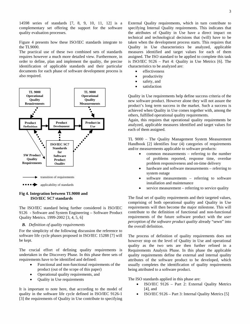
14598 series of standards [7, 8, 9, 10, 11, 12] is a complementary set offering the support for the software quality evaluation processes. Figure 4 presents how these ISO/IEC standards integrate to the TL9000. The practical use of these two combined sets of standards requires however a much more detailed view. Furthermore, in order to define, plan and implement the quality, the precise identification of applicable standards and their particular documents for each phase of software development process is also required.

Fig 4. Integration between TL9000 a ISO/IEC SC7 standards The ISO/IEC standard being further9126 - Software and System EngineeQuality Metrics. 1999-2002 [3, 4, 5, 6

B. Definition of quality requiremenFor the simplicity of the following dissoftware life cycle phases proposed inbe kept. The crucial effort of defining qundertaken in the Discovery Phase. Inrequirements have to be identified and

• Functional and non-functioproduct (out of the scope o

• Operational quality require• Quality in Use requirement

It is important to note here, that accquality in the software life cycle defi[3] the requirements of Quality in Use

External Quality requirements, which in turn contribute to specifying Internal Quality requirements. This indicates that the attributes of Quality in Use have a direct impact on technical and technological decisions that (will) have to be taken when the development process starts. This requires that Quality in Use characteristics be analyzed, applicable measures identified and target values for each of them assigned. The ISO standard to be applied to complete this task is ISO/IEC 9126 – Part 4: Quality in Use Metrics [6]. The characteristics to be analyzed are:

• effectiveness • productivity • safety, and • satisfaction

Quality in Use requirements help define success criteria of the new software product. However alone they will not assure the

ISO/IEC SC7 Standards

for Software Product Quality

SW Product Quality

Requirements

transition of requirements applicability of standards

Product Definition

Product Development

TL 9000 Operational

Quality Requirements M

TL 9000 Operational

Quality easurements

nd

considered is ISO/IEC ring – Software Product ]

ts cussion the reference to ISO/IEC 15288 [7] will

uality requirements is this phase three sets of defined: nal requirements of the f this paper) ments, and s

ording to the model of ned in ISO/IEC 9126-1 contribute to specifying

product’s long term success in the market. Such a success is achieved when Quality in Use comes together with, among the others, fulfilled operational quality requirements. Again, this requires that operational quality requirements be analyzed, applicable measures identified and target values for each of them assigned. TL 9000 – The Quality Management System Measurement Handbook [2] identifies four (4) categories of requirements and/or measurements applicable to software products:

• common measurements – referring to the number of problems reported, response time, overdue problem responsiveness and on-time delivery

• hardware and software measurements – referring to system outage

• software measurements – referring to software installation and maintenance

• service measurement – referring to service quality The final set of quality requirements and their targeted values, comprising of both operational quality and Quality in Use requirements will then become the major milestone. This will contribute to the definition of functional and non-functional requirements of the future software product with the user perception of the software product quality already “sewn” into the overall definition. The process of definition of quality requirements does not however stop on the level of Quality in Use and operational quality as the two sets are then further refined in a Requirements Analysis Phase. In this phase the applicable quality requirements define the external and internal quality attributes of the software product to be developed, which usually completes the identification of quality requirements being attributed to a software product. The ISO standards applied in this phase are:

• ISO/IEC 9126 – Part 2: External Quality Metrics [4], and

• ISO/IEC 9126 – Part 3: Internal Quality Metrics [5]

Product in Use

4

It has to be stressed here, that the attributes of both external and internal quality being defined in this phase make direct descendants of quality requirements previously set up in the Discovery phase, so the critic rule of traceability in software engineering is being conserved.

At this moment, with the process of the definition of software product quality properly done, the project of developing new software is, or at least should be, well equipped with identified and precise quality requirements and ready for execution. However, we now have the challenge of directing the product in a way that offers good guarantees that its quality goals will be achieved. In the next section we will argue that a different approach to quality control is needed in software development compared with traditional manufacturing.

III. OBTAINING AND CONTROLLING SOFTWARE PRODUCT QUALITY

Building software products is a profoundly intellectual activity. This provides a fundamental distinction between the activity of creating software products, and the activity of manufacturing goods. In the former, we are primarily concerned with controlling human creativity and directing a collaborative endeavor towards achieving some agreed goal (a software product that fulfils a specified need). In the latter we are interested in replicating an already agreed product, multiple times to within prescribed tolerances.

In both cases we have historically used a common vocabulary to express concepts that pertain to the “quality” of the respective products. Perhaps even more unjustifiably, many have endeavored to apply similar techniques of process control to attempt to achieve quality software products as are used to achieve quality hardware products. And yet, as we have argued, the two activities are fundamentally different.

In this section, we will argue that the application of process control methods using simple regression models has limited applicability to the development of software products, and introduce the requirements for a quality control method that is informed by rich causal models.

Fenton and Neil [1999] provide a detailed critique of software defect prediction models. The essential problem is the oversimplification that is generally associated with the use

of simple regression models. Typically, the search is for a simple relationship between some predictor and the number of defects delivered. Size or complexity measures are often used as such predictors. The result is a naïve model that could be represented by the graph of Figure 5.

The difficulty is that whilst such a model can be used to explain a data set obtained in a specific context, none has so far been subject to the form of controlled statistical experimentation needed to establish a causal relationship. Indeed, the analysis of Fenton and Neil suggests that these models fail to include all the causal or explanatory variables needed in order to make the models generalisable. Further strong empirical support for these arguments is demonstrated in [Fenton and Ohlsson, 2000].

As an example, in investigating the relationship between two variables such as S and D in Figure 5, one would at least wish to differentiate between a direct causal relationship and the influence of some common cause as a “hidden variable”. For example, we might hypothesise “Problem Complexity” (PC) as a common cause for our two variables S and D, Figure 6.

The model of Figure 5 can simulate the model of Figure 6 under certain circumstances. However, the latter has greater explanatory power, and can lead to quite a different interpretation of a set of data. One could take “Smoking” and “Higher Grades” at high school as an analogy. Just looking at the covariance between the two variables, we might see a correlation between smoking and achieving higher grades. However, if "Age" is then included in the model, we could

have a very different interpretation of the same data. As a student's age increases, so does the likelihood of their smoking. As they mature, their grades also typically improve. The covariance is explained. However, for any fixed age group, smokers may achieve lower grades than non-smokers.

We believe that the relationships between product and process attributes and numbers of defects are too complex to admit straightforward curve fitting models. In predicting defects discovered in a particular project, we would certainly

PC

S D

Figure 6: The influence of S on D is now mediated through a common cause PS. This model can behave in the same way as that of Figure 5, but only in certain specific circumstances.

S D

Figure 5: Graphical representation of a naïve regression model between some predictor S (typically a size measure), and the number of software defects D.

5

want to add additional variables to the model of Figure 6. For example, the number of defects discovered will depend on the effectiveness with which the software is tested. It may also depend on the level of detail of the specifications from which the test cases are derived, the care with which requirements have been managed during product development, and so on. We believe that graphical probabilistic models are the best candidate for situations with such a rich causal structure.

IV. A PROBABILISTIC MODEL FOR DEFECT PREDICTION Probabilistic models are a good candidate solution for an

effective model of software defect prediction (one aspect of quality control) for the following reasons:

1. They can easily model causal influences between variables in a specified domain;

2. The Bayesian approach enables statistical inference to be augmented by expert judgement in those areas of a problem domain where empirical data is sparse;

3. As a result of the above, it is possible to include variables in a software reliability model that correspond to process as well as product attributes;

4. Assigning probabilities to reliability predictions means that sound decision making approaches using classical decision theory can be supported.

Our goal was to build a module level defect prediction model that could then be evaluated against real project data from within the Philips Electronics group of business units. This model was built in a collaborative project between Philips Electronics and Agena Ltd (Fenton, Krause and Neil, 2001). Although it was not possible to use members of Philips' development organisations directly to perform extensive knowledge elicitation, Philips Research Laboratories (PRL) were able to act as a surrogate because of their experience from working directly with Philips business units. This had the added advantage that the probabilistic network could be built relatively quickly. However, the fact that the probability tables were in effect built from “rough” information sources and strengths of relations necessarily limits the precision of the model.

The remainder of this section will provide an overview of the model to indicate the product and process factors that are taken into account when a quality assessment is performed using it.

A. Overall structure of the probabilistic network The probabilistic network is executed using the generic

probabilistic inference engine Hugin (see http://www.hugin.com for further details). However, the size and complexity of the network were such that it was not realistic to attempt to build the network directly using the Hugin tool. Instead, Agena Ltd used two methods and tools that are built on top of the Hugin propagation engine:

The SERENE method and tool [SERENE, 1999], which enables: large networks to be built up from smaller ones in a

modular fashion; and, large probability tables to be built using pre-defined mathematical functions and probability distributions.

The IMPRESS method and tool [IMPRESS, 1999], which extends the SERENE tool by enabling users to generate complex probability distributions simply by drawing distribution shapes in a visual editor.

The resulting network takes account of a range of product and process factors from throughout the lifecycle of a software module. Because of the size of the model, it is impractical to display it in a single figure. Instead, we provide first a schematic view in terms of sub-nets (Figure 7). This modular structure is the actual decomposition that was used to build the network using the SERENE tool.

The main sub-nets in the high-level structure correspond to key software life-cycle phases in the development of a software module. Thus there are sub-nets representing the specification phase, the specification review phase, the design and coding phase and the various testing phases. Two further sub-nets cover the influence of requirements management on defect levels, and operational usage on defect discovery. The final defect density sub-net simply computes the industry standard defect density metric in terms of residual defects

Specification quality

Specification review

Requirements match

Design and codingprocess

Unit testing process

Independent testingprocess

Defect density

Operational usage

Specificationdefects

Residualspecification

defects

Newrequirements

Code defectsDesign doc quality

Residualdefects

Residualdefects

delivered

Module sizeSpec quality

Matchingrequirements

Intrinsiccomplexity

Integration testingprocess

Residualdefects

Design docquality

Figure 7: Overall network structure.

6

delivered divided by module size. This structure was developed using the software

development processes from a number of Philips development units as models. A common software development process is not currently in place within Philips. Hence the resulting structure is necessarily an abstraction. Again, this will limit the precision of the resulting predictions. Work is in progress to develop tools to enable the structure to be customised to specific development processes (http://www.modist.org.uk).

The arc labels in Figure 7 represent ‘joined’ nodes in the underlying sub-nets. This means that information about the variables representing these joined nodes is passed directly between sub-nets. For example, the specification quality and the defect density sub-nets are joined by an arc labelled ‘Module size’. This node is common to both sub-nets. As a result, information about the module size arising from the specification quality sub-net is passed directly to the defect density sub-net. We refer to ‘Module size’ as an ‘output node’ for the specification quality sub-net, and an ‘input node’ for the defect density sub-net. In the following sub-section we will show the details of one of the sub-nets.

B. The specification quality sub-net Figure 8 illustrates the Specification quality sub-net. In this

figure, the dark shaded nodes with dotted edges are output nodes, and the dark shaded ones with solid edges are input nodes. It can be explained in the following way: specification quality is influenced by three major factors:

• the intrinsic complexity of the module (this is the complexity of the requirements for the module, which

ranges from “very simple” to “very complex”); • the internal resources used, which is in turn defined in

terms of the staff quality (ranging from “poor” to “outstanding”), the document quality (meaning the quality of the initial requirements specification document, ranging from “very poor” to “very good”), and the schedule constraints which ranges from “very tight” to “very flexible”;

• the stability of the requirements, which in turn is defined in terms of the novelty of the module requirements (ranging from “very high” to “very low”) and the stakeholder involvement (ranging from “very low” to “very high”). The stability node is defined in such a way that low novelty makes stakeholder involvement irrelevant (Philips would have already built a similar relevant module), but otherwise stakeholder involvement is crucial.

The specification quality directly influences the number of specification defects (which is an output node with an ordinal scale that ranges from 0 to 10 – here “0” represents no defects, whilst “10” represents a complete rewrite of the document). Also, together with stability, specification quality influences the number of new requirements (also an output node with an ordinal scale ranging from 0 to 10) that will be introduced during the development and testing process. The other node in this sub-net is the output node module size, measured in Lines of Code (LOC). The position taken when constructing the model is that module size is conditionally dependent on intrinsic complexity (hence the link). However, although it is an indicator of such complexity the relationship is fairly weak

- the Node Probability Table (NPT) for this node models a shallow distribution. schedule document

quality staff

quality stakeholder involvement C. Some comments on the basic

probabilistic network The methods used to construct the model

have been illustrated in this section. The resulting network models the entire development and testing life-cycle of a typical software module. We believe it contains all the critical causal factors at an appropriate level of granularity, at least within the context of software development within Philips.

The node probability tables (NPTs) were built by eliciting probability distributions based on experience from within Philips. Some of these were based on historical records, others on subjective judgements. For most of the non-leaf nodes of the network the NPTs were too large to elicit all of the relevant probability distributions using expert judgement. Hence we used the novel techniques, that have been developed recently on the SERENE and IMPRESS projects, to extrapolate all the distributions

Figure 8: Specification quality sub-net.

new rqmnts

new rqmnts

novelty

stability

module size

specification quality

internal resources

intrinsic complexity

spec. defects

7

based on a small number of samples. By applying numerous consistency checks we believe that the resulting NPTs are a fair representation of experience within Philips.

As it stands, the network can be used to provide a range of predictions and “what-if” analyses at any stage during software development and testing. It can be used both for quality control and process improvement. However, two further areas of work were needed before the tool could be considered ready for extended trials. Firstly and most importantly, the network needed to be validated using real-world data. Secondly a more user-friendly interface needed to be engineered so that (a) the tool did not require users to have experience with probabilistic modelling techniques, and (b) a wider range of reporting functions could be provided. The validation exercise will be described in the next section in a way that illustrates how the probabilistic network was packaged to form the AID tool (AID for “Assess, Improve, Decide”).

V. VALIDATION OF THE AID TOOL

A. Method The Philips Software Centre (PSC), Bangalore, India, made

validation data available. We gratefully acknowledge their support in this way. PSC is a centre for excellence for software development within Philips, and so data was available from a wide diversity of projects from the various Business Divisions within PSC.

Data was collected from 28 projects from three Business

Divisions: Mainstream Consumer Electronics, Philips Medical Systems and Digital Networks. This gave a spread of different sizes and types of projects. Data was collected from three sources:

• Pre-release and post-release defect data was collected from the “Performance Indicators” database.

• More extensive project data was available from the Project Database.

• Completed questionnaires on selected projects.

In addition, the network was demonstrated in detail on a one to one basis to three experienced quality/test engineers to obtain their reaction to its behaviour under a number of hypothetical scenarios.

The data from each project was entered into the probabilistic model. For each project:

Figure 9: The entire AID network illustrated using a Windows Explorer style view.

1. The data available for all nodes prior to the Unit Test sub-net was entered first.

2. Available data for the Unit Test sub-net was then entered, with the exception of data for defects discovered and fixed.

3. If pre-release defect data was available, the predicted probability distribution for defects detected and fixed in the unit test phase was compared with the actual number of pre-release defects. No distinction was made between major and minor defects – total numbers were used throughout. The actual value for pre-release defects was then entered.

4. All further data for the test phases was then entered where available, with the exception of the number of defects found and fixed during independent testing (“post-release defects”). The predicted probability distribution for defects found and fixed in independent testing was compared with the actual value.

5. If available, the actual value for the number of defects found and fixed during independent testing was then entered. The prediction for the number of residual defects was then noted.

Unfortunately, data was not available to validate the operational usage sub-net. This will need data on field call-rates that is not currently available.

Given the size of the probabilistic network, this was insufficient data to perform rigorous statistical tests of validity. However, it was sufficient data to be able to confirm whether or not the network’s predictions were reliable enough to warrant recommending that a more extensive controlled trial be set up.

8

B. Summary of results of the validation exercise Overall there was a high degree of consistency between the

behaviour of the network and the data that was collected. However, a significant amount of data is needed in order to make reasonably precise predictions for a specific project. Extensive data (filled questionnaire, plus project data, plus defect data) was available for seven out of 28 candidate projects. These seven projects showed a similar degree of

consistency to the project that will be studied in the next sub-section. The remaining 21 projects show similar effects, but as the probability distributions are broader (and hence less precise) given the significant amounts of “missing” information, the results are supportive but less convincing than the seven studied in detail.

It must be emphasised that all defect data refers to the total of major and minor defects. Hence, residual defects may not result in a “failure” that is perceptible to a user. This is particularly the case for user-interface projects.

Note also that the detailed contents of the questionnaires are held in confidence. Hence we cannot publish an example of data entry for the early phases in the software life cycle. Defect data will be reported here, but we must keep the details of the project anonymous.

C. An example run of AID We will use screen shots of the AID Tool to illustrate both the questionnaire based user interface, and a typical validation run.

One of the concerns with the original network is that many of the nodes have values on a simple ordinal scale, range from “very good” to “very poor”. This leaves open the possibility that different users will apply different calibrations to these

scales. Hence the reliability of the predictions may vary, dependent on the specific user of the system. We address this by providing a questionnaire based front-end for the system. The ordinal values are then associated with specific question answers. The answers themselves are phrased as categorical, non-judgemental statements.

The screen in Figure 9 shows the entire network. The network is modularised so that a Windows Explorer style view can be used to navigate quickly around the network. Check-boxes are provided to indicate which questions have already been answered for a specific project.

The questions associated with a specific sub-net can then be displayed. A question is answered by selecting the alternative from the suggested answers that best matches the state of current project.

For this example project, answers were available for 13 of the 16 questions preceding “defects discovered and fixed during unit test”. Once the answers to these questions were entered, the predicted probability distribution for defects discovered and fixed during unit test had a mean of 149 and median of 125 (see Figure 10 – in this figure the monitor window has been displayed in order to

show the complete probability distribution for this prediction. Summary statistics can also be displayed.). The actual value was 122. Given that the probability distribution is skewed, the median is the most appropriate summary statistic, so we actually see an apparently very close agreement between predicted and actual values. This agreement was very surprising as although we were optimistic that the “qualitative behaviour” of the network to be transferable from organisation to organisation, we were expecting the scaling of the defect numbers to vary. Note, however, that the median is an imprecise estimate of the number of defects – it is the centre value of its associated bin on the histogram. So it might be more appropriate to quote a median of “100-150” in order to make the imprecision of the estimate explicit.

Figure 10: The prediction for defects discovered and fixed during Unit Test for project “Test 3”.

The actual value for defects discovered and fixed was entered. Answers for “staff quality” and “resources” were available for the Integration Test and Independent Test sub-networks. Once

9

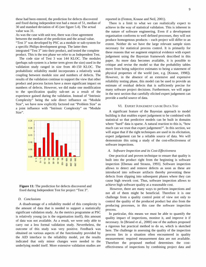
these had been entered, the prediction for defects discovered and fixed during independent test had a mean of 51, median of 30 and standard deviation of 45 (see figure 5.4). The actual value was 31. As was the case with unit test, there was close agreement between the median of the prediction and the actual value. “Test 3” was developed by PSC as a module or sub-system for a specific Philips development group. The latter then integrated “Test 3” into their product, and tested the complete product. This is the test phase we refer to as Independent Test.

The code size of Test 3 was 144 KLOC. The modules (perhaps sub-system is a better term given the size) used in the validation study ranged in size from 40-150 KLOC. The probabilistic reliability model incorporates a relatively weak coupling between module size and numbers of defects. The results of the validation continue to support the view that other product and process factors have a more significant impact on numbers of defects. However, we did make one modification to the specification quality sub-net as a result of the experience gained during the validation. Instead of “Intrinsic Complexity” being the sole direct influence on “Module Size”, we have now explicitly factored out “Problem Size” as a joint influence with “Intrinsic Complexity” on “Module Size”.

D. Conclusions A disadvantage of a reliability model of this complexity is

the amount of data that is needed to support a statistically significant validation study. As the metrics programme at PSC is relatively young (as is the organisation itself), this amount of data was not available. As a result, we were only able to carry out a less formal validation study. Nevertheless, the outcome of this study was very positive. Feedback was obtained on various aspects of the functionality provided by the AID interface to the reliability model, yet the results indicated that only minor changes were needed to the underlying model itself. More extensive validation studies are

reported in (Fenton, Krause and Neil, 2001). There is a limit to what we can realistically expect to

achieve in the way of statistical validation. This is inherent in the nature of software engineering. Even if a development organisation conforms to well defined processes, they will not produce homogenous products – each project will differ to an extent. Neither do we have the large relevant sample sizes necessary for statistical process control. It is primarily for these reasons that we augment empirical evidence with expert judgement using the Bayesian framework described in this paper. As more data becomes available, it is possible to critique and revise the model so that the probability tables move from being subjective estimates to being a statement of physical properties of the world (see, e.g. [Krause, 1998]). However, in the absence of an extensive and expensive reliability testing phase, this model can be used to provide an estimate of residual defects that is sufficiently precise for many software project decisions. Furthermore, we will argue in the next section that carefully elicited expert judgement can provide a useful source of data.

VI. EXPERT JUDGEMENT CAN BE DATA TOO A significant feature of the Bayesian approach to model

building is that enables expert judgement to be combined with statistical so that predictive models can be built in domains where “hard” data is sparse. A natural reaction to this is, “how much can we trust that expert judgement?”. In this section, we will argue that if the right techniques are used in its elicitation, expert judgement can be a reliable source of data. We will demonstrate this using a study of the cost-effectiveness of software inspections.

A. Software Inspection and its Cost-Effectiveness One practical and proven technique to ensure that quality is

built into the product right from the beginning is software inspection [Ebenau and Strauss, 1993]. Software inspection allows to detect and remove defects as soon as these are introduced into software artifacts thereby preventing these defects from slipping into subsequent phases where they can cause high rework cost. Thus, software inspection allows to achieve high software quality at a reasonable cost.

However, there are many ways to perform inspections and not all of them might be beneficial. Therefore it is one challenge from a quality control point of view not only to control the quality of the produced product but also from the producing processes, in this case the software inspection process.

In particular, this means we must be able to quantify the quality impact of inspections, monitor it, and improve it if necessary. In [Briand et al., 2000] one of the authors proposed a rigorous but practical method to do so, which is sketched here. The challenge in assessing the quality of the inspection process lies in a situation often encountered in quality measurement: required measurement data are not available. Therefore the proposed method determines the cost-effectiveness of inspections by combining project data and

Figure 11: The prediction for defects discovered and fixed during Independent Test for project “Test 3”.

10

expert opinion. 1) Measuring Inspection Cost Effectiveness

In order to control the quality of the inspection process, we must first quantify the quality criterion we are interested in. The quantitative benefit of inspections is the saved rework effort. To capture this, we assess therefore the cost-effectiveness of inspections

In order to measure cost-effectiveness the cost-effectiveness model initially proposed by Kusumoto [Kusumoto et al., 1992] is selected. However, the original model is re-expressed and generalized to multiple inspection activities in order to relax some of its assumptions. For more details regarding this selection the interested reader is referred to the discussions in [Briand et. al., 1998b] and [Briand et. al., 2000].

Generally, the model defines cost-effectiveness (CE) as:

sinspectiont_without_defect_cospotential_pectionsmed_by_inscost_consutions_by_inspecCost_savedE −

=C

The total potential defect costs are the defect rework cost that would have been incurred if no inspections had taken place. The cost consumed by inspections is the cost spent on performing inspections, while the cost saved by inspections estimate the cost saved in later phases due to the defect detection in inspections.

Thus, the model is intuitive as it can be interpreted as the percentage of defect rework costs that are saved due to inspections. With this definition cost-effectiveness is stated in terms of effort savings and can be compared across different types of inspections (e.g., between inspections of different projects or in different phases of the life-cyle).

However, expressed in the form above, the model requires data that is difficult to obtain. Therefore, it is our approach to express the model in terms of parameters that can either be easily obtained through data collection during project performance or through the elicitation of expert opinion.

2) On the Use of Expert opinion There are many reasons why expert opinion may be needed.

One of these reasons, that we face here, is when information regarding a phenomenon cannot be collected by any other affordable means (measurements, observations, experimentation) or that the required data is simply not being collected. The question is now, especially when looking at the problem from a scientific perspective, whether expert data are valid data.

It might be argued that expert data are soft data in the sense that they incorporate the assumptions and interpretation of the experts [17]. Specifically, expert data are subject to bias, uncertainty, and incompleteness. However, these problems can be prevented and controlled. Generally, the aim of expert knowledge elicitation techniques is to prevent the problems to the maximum extent possible, detect bias when it occurs, and model uncertainty. Elicitation techniques achieve this by carefully selecting experts, designing the mode of data collection and the interview procedure, and quantifying uncertainty in experts’ responses. Thus, expert judgment can be defined as data gathered formally, in a structured manner, and in accordance with research on human cognition and

communication [17]. To summarize, we believe that expert judgment is valid

data and is comparable to other data. Expert judgment has been used in similar ways and with success in other fields such as nuclear engineering (risk models) [14] and policy decision making [20], and in software engineering for cost estimation purposes [2], [12].

3) Expert Elicitation Techniques Bias and uncertainty are two important aspects (among

others) that have to be addressed in expert opinion elicitation. In the following these two concepts are explained in more detail.

a) Bias During elicitation, the experts will perform four cognitive

tasks. They must comprehend the wording and the context questions asked. Then they must remember relevant information to answer each question. By processing this information the experts identify an answer, which is said to be “internal” as it is in the expert’s own representation mode. At this stage, people typically use mental shortcuts called heuristics to help integrate and process the information [Kahneman et al., 1982]. Finally, the internal answer has to be translated into the format requested by the interviewer (i.e., the so-called response mode).

In each of these steps, especially in applying the heuristics, systematic errors can occur, which would distort the estimate. To obtain reliable data it is therefore necessary to anticipate these biases and design and monitor the elicitation accordingly [Meyer and Booker, 1991]. This involves to anticipate which biases are likely to occur in the planned elicitation and re-design the planned elicitation to make it less prone to the anticipated biases. During the elicitation the experts need to be made aware of the potential intrusion of particular biases. Finally, during elicitation, the interviewer monitors the experts' body language and the verbalized thoughts of the expert for the occurrence of bias

b) Uncertainty Often it is impossible to ask the experts for a single value

for an estimate. One reason is that subjective estimates are inherently uncertain. This uncertainty stems from the experts’ lack of knowledge on the exact value for a parameter. Providing an exact answer might be impossible since experts may not know the exact value or since the parameter value may actually vary with circumstances. For example, it is obvious that the cost of defect correction does not warrant a unique value but a probability distribution, since the correction effort can vary with the type of defect.

To explicitly capture this uncertainty the experts can give their answers in the form of a probability distribution (i.e., as a response mode as it will be introduced later). With such a distribution the experts are able to quantify their uncertainty. The probability distribution most often used in expert opinion

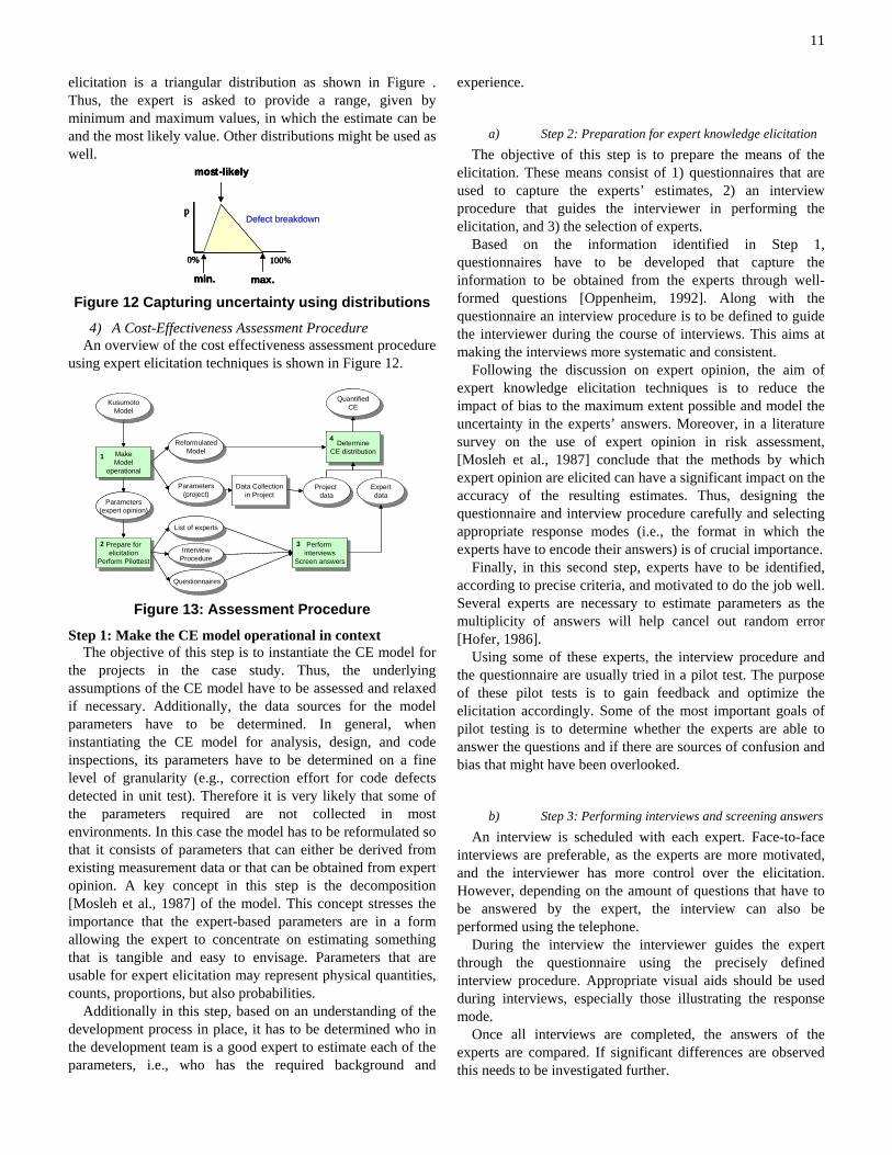
11

elicitation is a triangular distribution as shown in Figure . Thus, the expert is asked to provide a range, given by minimum and maximum values, in which the estimate can be and the most likely value. Other distributions might be used as well.

Defect breakdown

most-likely

max.min.

100%0%

pDefect breakdown

most-likely

max.min.

100%0%

p

most-likely

max.min.

100%0%

p

Figure 12 Capturing uncertainty using distributions

4) A Cost-Effectiveness Assessment Procedure An overview of the cost effectiveness assessment procedure

using expert elicitation techniques is shown in Figure 12.

MakeModel

operational

MakeModel

operational

Prepare forelicitation

Perform Pilottest

Prepare forelicitation

Perform Pilottest

Data Collectionin Project

Data Collectionin Project

DetermineCE distributionDetermine

CE distribution

KusumotoModel

KusumotoModel

ReformulatedModel

ReformulatedModel

Parameters(project)

Parameters(project)

Parameters(expert opinion)Parameters

(expert opinion)

QuestionnairesQuestionnaires

InterviewProcedureInterview

Procedure

List of expertsList of experts

Project data

Project data

Expertdata

Expertdata

Perform interviews

Screen answers

Perform interviews

Screen answers

QuantifiedCE

QuantifiedCE

1

2 3

4

MakeModel

operational

MakeModel

operational

Prepare forelicitation

Perform Pilottest

Prepare forelicitation

Perform Pilottest

Data Collectionin Project

Data Collectionin Project

DetermineCE distributionDetermine

CE distribution

KusumotoModel

KusumotoModel

ReformulatedModel

ReformulatedModel

Parameters(project)

Parameters(project)

Parameters(expert opinion)Parameters

(expert opinion)

QuestionnairesQuestionnaires

InterviewProcedureInterview

Procedure

List of expertsList of experts

Project data

Project data

Expertdata

Expertdata

Perform interviews

Screen answers

Perform interviews

Screen answers

QuantifiedCE

QuantifiedCE

1

2 3

4

Figure 13: Assessment Procedure

Step 1: Make the CE model operational in context The objective of this step is to instantiate the CE model for

the projects in the case study. Thus, the underlying assumptions of the CE model have to be assessed and relaxed if necessary. Additionally, the data sources for the model parameters have to be determined. In general, when instantiating the CE model for analysis, design, and code inspections, its parameters have to be determined on a fine level of granularity (e.g., correction effort for code defects detected in unit test). Therefore it is very likely that some of the parameters required are not collected in most environments. In this case the model has to be reformulated so that it consists of parameters that can either be derived from existing measurement data or that can be obtained from expert opinion. A key concept in this step is the decomposition [Mosleh et al., 1987] of the model. This concept stresses the importance that the expert-based parameters are in a form allowing the expert to concentrate on estimating something that is tangible and easy to envisage. Parameters that are usable for expert elicitation may represent physical quantities, counts, proportions, but also probabilities.

Additionally in this step, based on an understanding of the development process in place, it has to be determined who in the development team is a good expert to estimate each of the parameters, i.e., who has the required background and

experience.

a) Step 2: Preparation for expert knowledge elicitation The objective of this step is to prepare the means of the

elicitation. These means consist of 1) questionnaires that are used to capture the experts’ estimates, 2) an interview procedure that guides the interviewer in performing the elicitation, and 3) the selection of experts.

Based on the information identified in Step 1, questionnaires have to be developed that capture the information to be obtained from the experts through well-formed questions [Oppenheim, 1992]. Along with the questionnaire an interview procedure is to be defined to guide the interviewer during the course of interviews. This aims at making the interviews more systematic and consistent.

Following the discussion on expert opinion, the aim of expert knowledge elicitation techniques is to reduce the impact of bias to the maximum extent possible and model the uncertainty in the experts’ answers. Moreover, in a literature survey on the use of expert opinion in risk assessment, [Mosleh et al., 1987] conclude that the methods by which expert opinion are elicited can have a significant impact on the accuracy of the resulting estimates. Thus, designing the questionnaire and interview procedure carefully and selecting appropriate response modes (i.e., the format in which the experts have to encode their answers) is of crucial importance.

Finally, in this second step, experts have to be identified, according to precise criteria, and motivated to do the job well. Several experts are necessary to estimate parameters as the multiplicity of answers will help cancel out random error [Hofer, 1986].

Using some of these experts, the interview procedure and the questionnaire are usually tried in a pilot test. The purpose of these pilot tests is to gain feedback and optimize the elicitation accordingly. Some of the most important goals of pilot testing is to determine whether the experts are able to answer the questions and if there are sources of confusion and bias that might have been overlooked.

b) Step 3: Performing interviews and screening answers An interview is scheduled with each expert. Face-to-face

interviews are preferable, as the experts are more motivated, and the interviewer has more control over the elicitation. However, depending on the amount of questions that have to be answered by the expert, the interview can also be performed using the telephone.

During the interview the interviewer guides the expert through the questionnaire using the precisely defined interview procedure. Appropriate visual aids should be used during interviews, especially those illustrating the response mode.

Once all interviews are completed, the answers of the experts are compared. If significant differences are observed this needs to be investigated further.

12

c) Step 4: Compute cost-effectiveness The objective of the fourth step is to determine the cost-

effectiveness of inspections, in the environment under study, and according to the CE model. Step 1 produces operational CE models for each inspection phase, including the description of their parameters. Together with the experts’ responses, the cost-effectiveness is then computed as illustrated in Figure 14 with design inspections.

For those parameters that can be determined from measurement data, the values are computed from either inspection or test data. For those parameters that are to be estimated by expert knowledge elicitation, the estimates of different experts for each question have to be aggregated.

Since the estimates of the experts were actually probability distributions, also estimate a probability distribution for the cost-effectiveness is computed. This distribution captures the inherent uncertainty in the cost-effectiveness of inspections. This uncertainty has two sources: the uncertainty in the experts’ estimates and the inherent variation of cost-effectiveness across inspections. An important methodological point in presenting the results of any expert opinion study is to make explicit the underlying uncertainty of the results [Hora and Iman, 1989]. A probability distribution of the cost-effectiveness takes this aspect automatically into account.

CE

Model

CE

(af ,A

) cost-effectivenessdistribution

pDI,D

Proportion of design defects in design inspections?

aggregation

nD

I,D =nD *p

DI,D

estimatemodel parameter

MC-simulation of CE model

Data

Number of defects indesign inspections?nDI=200

Project data

InterviewsC

E M

odel C

E(a

f ,A) cost-effectiveness

distribution

pDI,D

Proportion of design defects in design inspections?

aggregation

nD

I,D =nD *p

DI,D

estimatemodel parameter

MC-simulation of CE model

Data

Number of defects indesign inspections?nDI=200Data

Number of defects indesign inspections?nDI=200

Project data

Interviews

Figure 14: Determining CE

Monte-Carlo (MC-) Simulation is a convenient way of performing the aggregation of experts’ data [Vose, 1996] and the computation of the cost-effectiveness distribution. During one simulation run, a value for each input parameter is sampled from the experts’ probability distributions. The set of sampled values forms a possible scenario, which is used as input to the model to compute the corresponding cost-effectiveness value. Repeating this procedure 1000 times provides 1000 cost-effectiveness values which form a distribution.

5) Experience with the proposed method The proposed method was developed specifically for a

development organization and validated in a carefully designed case study, which took place in a business unit of Siemens AG, Germany, that is developing products and services for mobile communication and intelligent networks [Briand et al., 2000].

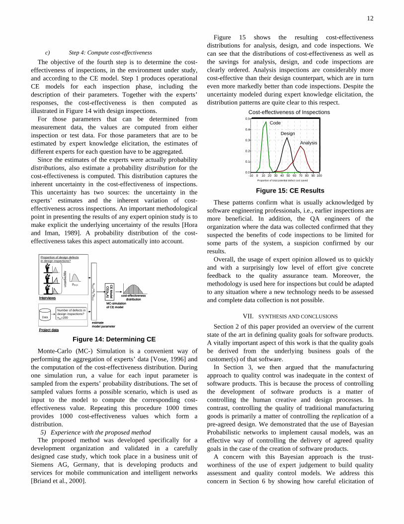
Figure 15 shows the resulting cost-effectiveness distributions for analysis, design, and code inspections. We can see that the distributions of cost-effectiveness as well as the savings for analysis, design, and code inspections are clearly ordered. Analysis inspections are considerably more cost-effective than their design counterpart, which are in turn even more markedly better than code inspections. Despite the uncertainty modeled during expert knowledge elicitation, the distribution patterns are quite clear to this respect.

Cost-effectiveness of Inspections

Legends:

Proportion of total potential defect cost saved

0.0

0.1

0.2

0.3

0.4

0.5

-10 0 10 20 30 40 50 60 70 80 90 100

C21/ Analyse RevC11/ Code ReviewC19/ Design Revi

Analysis

Design

Code

Cost-effectiveness of Inspections

Legends:

Proportion of total potential defect cost saved

0.0

0.1

0.2

0.3

0.4

0.5

-10 0 10 20 30 40 50 60 70 80 90 100

C21/ Analyse RevC11/ Code ReviewC19/ Design Revi

Analysis

Design

Code

Figure 15: CE Results

These patterns confirm what is usually acknowledged by software engineering professionals, i.e., earlier inspections are more beneficial. In addition, the QA engineers of the organization where the data was collected confirmed that they suspected the benefits of code inspections to be limited for some parts of the system, a suspicion confirmed by our results.

Overall, the usage of expert opinion allowed us to quickly and with a surprisingly low level of effort give concrete feedback to the quality assurance team. Moreover, the methodology is used here for inspections but could be adapted to any situation where a new technology needs to be assessed and complete data collection is not possible.

VII. SYNTHESIS AND CONCLUSIONS Section 2 of this paper provided an overview of the current

state of the art in defining quality goals for software products. A vitally important aspect of this work is that the quality goals be derived from the underlying business goals of the customer(s) of that software.

In Section 3, we then argued that the manufacturing approach to quality control was inadequate in the context of software products. This is because the process of controlling the development of software products is a matter of controlling the human creative and design processes. In contrast, controlling the quality of traditional manufacturing goods is primarily a matter of controlling the replication of a pre-agreed design. We demonstrated that the use of Bayesian Probabilistic networks to implement causal models, was an effective way of controlling the delivery of agreed quality goals in the case of the creation of software products.

A concern with this Bayesian approach is the trust-worthiness of the use of expert judgement to build quality assessment and quality control models. We address this concern in Section 6 by showing how careful elicitation of

13

expert judgement can be a reliable and valuable source of data.

It is our firm belief that this synthesis of three strands of research in software quality provides a foundation for an effective method of quality control for software related products.

APPENDIX For the benefit of those who are unfamiliar with probability

theory, we provide in this appendix a brief introduction to probabilistic causal models.

A. Conditional probability Probabilities conform to three basic axioms: • p(A), the probability of an event

(outcome/consequence…), A, is a number between 0 and 1;

• p(A)=0 means A is impossible, p(A)=1 means A is certain;

• p(A or B) = p(A) + p(B) provided A and B are disjoint. However, merely to refer to the probability p(H) of an event or hypothesis is an oversimplification. In general, probabilities are context sensitive. For example, the probability of suffering from certain forms of cancer is higher in Europe than it is in Asia. Strictly, the probability of any event or hypothesis is conditional on the available evidence or current context. This can be made explicit by the notation p(H | E), which is read as “the probability of H given the evidence E”. In the coin example, H would be a “heads” event and E an explicit reference to the evidence that the coin is a fair one. If there was evidence E' that the coin was double sided heads, then we would have p(H | E') = 1.0. As soon as we start thinking in terms of conditional probabilities, we begin to need to think about the structure of problems as well as the assignment of numbers. To say that the probability of an hypothesis is conditional on one or more items is to identify the information relevant to the problem at hand. To say that the identification of an item of evidence influences the probability of an hypothesis being valid is to place a directionality on the links between evidences and hypotheses. Often a direction corresponding to causal influence can be the most meaningful. For example, in medical diagnosis one can

in a certain sense say that measles “causes” red spots (there might be other causes). So, as well as assigning a value to the conditional p(‘red spots’ | measles), one might also wish to

provide an explicit graphical representation of the problem. In this case it is very simple (Figure A.1). Note that to say that p(‘red spots’ | measles) = p means that we can assign probability p to ‘red spots’ if measles is observed and only measles is observed. If any further evidence E is observed, then we will be required to determine p(‘red spots’ | measles, E). The comma inside the parentheses denotes conjunction. Building up a graphical representation can be a great aid in framing a problem. A significant recent advance in probability theory has been the demonstration of a formal equivalence between the structure of a graphical model and the dependencies that are expressed by a numerical probability distribution. In numerical terms, we say that event A is independent of event B if observation of B makes no difference to the probability that A will occur: p(A | B) = p(A). In graphical terms we indicate that A is independent of B by the absence of any direct arrow between the nodes representing A and B in a graphical model. So far, we have concentrated on the static aspects of assessing probabilities and indicating influences. However, probability is a dynamic theory; it provides a mechanism for coherently revising the probabilities of events as evidence becomes available. Conditional probability and Bayes’ Theorem play a central role in this. We will use a simple example to illustrate Bayesian updating, and then introduce Bayes’ Theorem in the next section. Suppose we are interested in the number of defects that are detected and fixed in a certain testing phase. If the software under test had been developed to high standards, perhaps undergoing formal reviews before release to the test phase, then the high quality of the software would in a sense “cause” a low number of defects to be detected in the test phase. However, if the testing were ineffective and superficial, then this would provide an alternative cause for a low number of defects being detected during the test phase. (This was precisely the common empirical scenario identified in [Fenton and Ohlsson, 2000]).

red spots

measles

Figure A.1: A very simple probabilistic k

14

This situation can be represented by the simple graphical model of figure A.2. Here the nodes in the graph could represent simple binary variables with states “low” and “high”, perhaps. However, in general a node may have many alternative states or even represent a continuous variable. We will stay with the binary states for ease of discussion. It can be helpful to think of figure A.2 as a fragment of a much larger model. In particular, the node SQ (“Software Quality”) could be a synthesis of, for example: review effectiveness; developer’s skill level; quality of input specifications; and, resource availability. With appropriate probability assignments to this model, a variety of reasoning styles can be modelled. A straightforward reasoning from cause to effect is possible. If TE (test effectiveness) is “low”, then the model will predict that DD (defects discovered and fixed) will also be low. If earlier evidence indicates SQ (software quality) is “high”, then again DD will be “low”. However, an important feature is that although conditional probabilities may have been assessed in terms of effect given cause, Bayes’ rule enables inference to be performed in the “reverse” direction – to provide the probabilities of potential causes given the observation of some effect. In this case, if DD is observed to be “low” the model will tell us that low test effectiveness or high software quality are possible explanations (perhaps with an indication as to which one is the most likely explanation). The concept of “explaining away” will also be modelled. For example, if we also have independent evidence that the software quality was indeed high, then this will provide sufficient explanation of the observed value for DD and the probability that test effectiveness was low will be reduced. This situation can be more formally summarised as follows. If we have no knowledge of the state DD then nodes TE and SQ are marginally independent – knowledge of the state of one will not influence the probability of the other being in any of its possible states. However, nodes TE and SQ are conditionally dependent given DD – once the state of DD is

known there is an influence (via DD) between TE and SQ as described above.

TE SQ We will see in the next section that models of complex situations can be built up by composing together relatively simple local sub-models of the above kind (See also [Neil et al, 2000]). This is enormously valuable. Without being able to structure a problem in this way it can be virtually impossible to assess probability distributions over large numbers of variables. In addition, the computational problem of updating such a probability distribution given new evidence would be intractable.

DD B. Bayes’ theorem and graphical models

As indicated in the previous section, probability is a dynamic theory; it provides a mechanism for coherently revising the probabilities of events as evidence becomes available. Bayes’ theorem is a fundamental component of the dynamic aspects. As mentioned earlier, we write p(A | B) to represent the probability of some event (an hypothesis) conditional on the occurrence of some event B (evidence). If we are

counting sample events from some universe Ω, then we are interested in the fraction of events B for which A is also true. In effect we are focusing attention from the universe Ω to a restricted subset in which B holds. From this it should be clear that (with the comma denoting conjunction of events):

Figure A.2: Some subtle interactions between variables captured in a simple graphical model. Node TE represents “Test Effectiveness”, SQ represents “Software Quality” and DD represents “Defects Detected and Fixed”.

)(),()|(

BpBApBAp =

This is the simplest form of Bayes’ rule. However, it is more usually rewritten in a form that tells us how to obtain a posterior probability in a hypothesis A after observation of some evidence B, given the prior probability in A and the likelihood of observing B were A to be the case:

)()()|(

)|(Bp

ApABpBAp =

Z

X Y

This theorem is of immense practical importance. It means that we can reason both in a forward direction from causes to effects, and in a reverse direction (via Bayes’ rule) from effects to possible causes. That is, both deductive and abductive modes of reasoning are possible.

Figure A.3: X is conditionally independent of Y given Z.

15

However, two significant problems need to be addressed. Although in principle we can use generalisations of Bayes’ rule to update probability distributions over sets of variables, in practice: 1) Eliciting probability distributions over sets of variables is

a major problem. For example, suppose we had a problem describable by seven variables each with two possible states. Then we will need to elicit (27-1) distinct values in order to be able to define the probability distribution completely. As can be seen, the problem of knowledge elicitation is intractable in the general case.

2) The computations required to update a probability distribution over a set of variables are similarly intractable in the general case.

Up until the late 1980’s, these two problems were major obstacles to the rigorous use of probabilistic methods in computer based reasoning models. However, work initiated by Lauritzen and Spiegelhalter [1988] and Pearl [1988] provided a resolution to these problems for a wide class of problems. This work related the independence conditions described in graphical models to factorisations of the joint distributions over sets of variables. We have already seen some simple examples of such models in the previous section. In probabilistic terms, two variables X and Y are independent if p(X,Y) = p(X)p(Y) – the probability distribution over the two variables factorises into two independent distributions. This is expressed in a graphic by the absence of a direct arrow expressing influence between the two variables. We could introduce a third variable Z, say, and state that “X is conditionally independent of Y given Z”. This is expressed graphically in Figure A.3. An expression of this in terms of probability distributions is: p(X,Y | Z) = p(X | Z)p(Y | Z) A significant feature of the graphical structure of Figure A.3 is that we can now decompose the joint probability distribution for the variables X, Y and Z into the product of terms involving at most two variables: p(X,Y,Z) = p(X | Z)p(Y | Z)p(Z) In a similar way, we can decompose the joint probability distribution for the variables associated with the nodes DD, TE and SQ of Figure 4.2 as p(DD, TE, SQ) = p(DD | TE,SQ)p(TE)p(SQ) This gives us a series of example cases where a graph has admitted a simple factorisation of the corresponding joint probability distribution. If the graph is directed (the arrows all have an associated direction) and there are no cycles in the graph, then this property is a general one. Such graphs are called Directed Acyclic Graphs (DAGs). Using a slightly imprecise notation for simplicity, we have [Lauritzen and Spiegelhalter, 1988]: Proposition Let U = X1, X2, …, Xn have an associated DAG G. Then the joint probability distribution p(U) admits a direct factorisation:

))(|()(1

∏=

=n

i

ii XpaXpUp

Here pa(Xi) denotes a value assignment to the parents of Xi. (If an arrow in a graph is directed from A to B, then A is a parent node and B a child node). The net result is that the probability distribution for a large set of variables may be represented by a product of the conditional probability relationships between small clusters of semantically related propositions. Now, instead of needing to elicit a joint probability distribution over a set of complex events, the problem is broken down into the assessment of these conditional probabilities as parameters of the graphical representation. The lessons from this section can be summarised quite succinctly. First, graphs may be used to represent qualitative influences in a domain. Secondly, the conditional independence statements implied by the graph can be used to factorise the associated probability distribution. This factorisation can then be exploited to (a) ease the problem eliciting the global probability distribution, and (b) allow the development of computationally efficient algorithms for updating probabilities on the receipt of evidence. We will now describe how these techniques have been exploited to produce a probabilistic model for software defect prediction.

ACKNOWLEDGMENT Paul Krause thanks the support of Norman Fenton and

Martin Neil of Agena Limited, UK (www.agena.co.uk) who have been instrumental in the development of many of the ideas in this paper.

REFERENCES [1] TL9000 Quality Management System Requirements Handbook,

Release 3.0, QuEST Forum 2001 [2] TL9000 Quality Management System Measurements Handbook,

Release 3.0, QuEST Forum 2001 [3] ISO/IEC 9126 – Software and System Engineering – Product

quality – Part 1: Quality model. 1999-2002 [4] ISO/IEC 9126 – Software and System Engineering – Product

quality – Part 2: External Quality Metrics. 1999-2002 [5] ISO/IEC 9126 – Software and System Engineering – Product

quality – Part 3: Internal Quality Metrics. 1999-2002 [6] ISO/IEC 9126 – Software and System Engineering – Product

quality – Part 4: Quality in Use Metrics. 1999-2002 [7] ISO/IEC 15288 - Software and System Engineering – Life Cycle

Management – System Life Cycle Processes, 2002 [8] L. Briand, K. El Emam, and F. Bomarius, COBRA: A Hybrid

Method for Software Cost Estimation, Benchmarking, and Risk Assessment, in Proceedings of the 20th International Conference on Software Engineering, pp. 390-399, 1998.

[9] L. Briand, K. El Emam, O. Laitenberger, and T. Fussbroich, Using Simulation to Build Inspection Efficiency Benchmarks for Development Projects, in Proceedings of the 20th International Conference on Software Engineering, pp. 340-349, 1998.

[10] L. Briand, B. Freimut, F. Vollei, Assessing the Cost-Effectiveness of Inspections by Combining Project Data and Expert Opinion, Proceedings of the 11th International

16

Symposium on Software Reliability Engineering, pp 124-135, 2000.

[11] R. G. Ebenau and S. H. Strauss, Software Inspection Process., McGraw Hill, 1993.

[12] M. Höst and C. Wohlin, A Subjective Effort Estimation Experiment, International Journal of Information and Software Technology, Vol. 39, No. 11, pp. 755-762, 1997.

[13] E. Hofer, On surveys of expert opinion, Nuclear Engineering and Design, vol. 93, no. 2-3, pp. 153-160, 1986.

[14] S.C. Hora and R.L. Iman, Expert opinion in risk analysis: the NUREG-1150 methodology, Nuclear Science and Engineering, vol. 102, pp. 323-331, Aug. 1989.

[15] D. Kahneman, P. Slovic, and A. Tversky, eds., Judgement under uncertainty: Heuristics and biases. Cambridge University Press, 1982.

[16] S. Kusumoto, K. Matsumoto, T. Kikuno, and K. Torii, A new metric for cost-effectiveness of software reviews, IEICE Transactions on Information and Systems, vol. E75-D, no. 5, pp. 674-680, 1992.

[17] M. A. Meyer and J. M. Booker, Elicitating and Analyzing Expert Judgement: A Practical Guide., Academic Press, Ltd., 1991.

[18] A. Mosleh, V.M. Bier, and G. Apostolakis, The elicitation and use of expert opinion in risk assessment: a critical review, in Probabilistic Safety Assessment and Risk Management: PSA '87, vol. 1 of 3, pp. 152-158, 1987.

[19] A.N. Oppenheim, Questionnaire Design, Interviewing and Attitude Measurement. Pinter Publishers, 1992.

[20] T. Saaty, The Analytic Hierarchy Process, McGraw-Hill, 1990. [21] D. Vose, Quantitative Risk Analysis: A Guide to Monte Carlo

Simulation Modelling. John Wiley Sons, 1996. [22] Agena Ltd, “Bayesian Belief Nets”,

http://www.agena.co.uk/bbn_article/bbns.html, 1999. [23] N.E. Fenton and S.L. Pfleeger, Software Metrics: A Rigorous

and Practical Approach, (2nd Edition), PWS Publishing Company, 1997.

[24] N. Fenton and M. Neil “A Critique of Software Defect Prediction Research”, IEEE Trans. Software Eng., 25, No.5, 1999.

[25] N. Fenton and N. Ohlsson “Quantitative analysis of faults and failures in a complex software system”, IEEE Trans. Software Eng., 26, 797-814, 2000.

[26] HUGIN Expert Brochure. Hugin Expert A/S, P.O. Box 8201 DK-9220 Aalborg, Denmark, 1998.

[27] IMPRESS (IMproving the software PRocESS using bayesian nets) EPSRC Project GR/L06683, http://www.csr.city.ac.uk/csr_city/projects/impress.html, 1999.

[28] P.J. Krause. “Learning Probabilistic Networks”, Knowledge Engineering Review, 13, 321-351, 1998

[29] S.L. Lauritzen and D.J. Spiegelhalter, “Local computations with probabilities on graphical structures and their application to expert systems (with discussion)” J. Roy. Stat. Soc. Ser B 50, pp. 157-224, 1988.

[30] N. Lewis, “Continuous process improvement using Bayesian Belief Networks. The lessons to be learnt”. Proceedings of the twenty forth international conference on Computers and Industrial Engineering. Brunel University. 9th-11th September, 1998.

[31] McCall, P.K. Richards and G.F. Walters, Factors in software quality. Volumes 1, 2 and 3. Springfield Va., NTIS, AD/A-049-014/015/055, 1977.

[32] J. Musa, Software Reliability Engineering, McGraw Hill, 1999. [33] M. Neil, B. Littlewood and N. Fenton, “Applying Bayesian

Belief Networks to Systems Dependability Assessment”. Proceedings of Safety Critical Systems Club Symposium, Leeds, Published by Springer-Verlag, 6-8 February 1996.

[34] M. Neil, N. Fenton and L. Nielson, “Building large-scale Bayesian Networks”, Knowledge Engineering Review, to appear 2000.

[35] J. Pearl, Probabilistic Reasoning in Intelligent Systems: Networks of Plausible Inference Morgan Kauffman, 1988. (Revised in 1997)

[36] SERENE consortium, “SERENE (SafEty and Risk Evaluation using bayesian Nets): Method Manual”, ESPRIT Project 22187, http://www.dcs.qmw.ac.uk/~norman /serene.htm, 1999.