New Financial Activity Indexes: Early Warning System for Financial Imbalances in Japan Yuichiro Ito* yuuichirou.itou@boj.or.jp Tomiyuki Kitamura* tomiyuki.kitamura@boj.or.jp Koji Nakamura* kouji.nakamura@boj.or.jp

Takashi Nakazawa ** takashi.nakazawa@boj.or.jp

No.14-E-7 April 2014

Bank of Japan 2-1-1 Nihonbashi-Hongokucho, Chuo-ku, Tokyo 103-0021, Japan

* Financial System and Bank Examination Department ** Financial System and Bank Examination Department (currently Niigata Branch)

Papers in the Bank of Japan Working Paper Series are circulated in order to stimulate discussion and comments. Views expressed are those of authors and do not necessarily reflect those of the Bank. If you have any comment or question on the working paper series, please contact each author.

When making a copy or reproduction of the content for commercial purposes, please contact the Public Relations Department (post.prd8@boj.or.jp) at the Bank in advance to request permission. When making a copy or reproduction, the source, Bank of Japan Working Paper Series, should explicitly be credited.

Bank of Japan Working Paper Series

1

NEW FINANCIAL ACTIVITY INDEXES:

EARLY WARNING SYSTEM FOR FINANCIAL IMBALANCES IN JAPAN*

Yuichiro Ito,† Tomiyuki Kitamura,‡ Koji Nakamura,§ and Takashi Nakazawa**

April, 2014

Abstract

This paper describes Financial Activity Indexes (FAIXs), early warning system for

financial imbalances in Japan. We introduced the first version of FAIXs in 2012 and

revise FAIXs this time. First, we sort the candidate financial indicators into 14

categories. Second, in each category, we examine the usefulness of candidate indicators

from two perspectives: (a) whether the indicator can detect the overheating of financial

activities in the Japan's Heisei bubble period, which occurred around the late 1980s and

had a major impact on Japan's economy and financial activities; and (b) whether the

indicator successfully minimizes various statistical errors involved in forecasting future

events. In the examination, multiple possibilities are explored with respect to methods

used for extracting trends from indicators and thresholds employed for assessing that

the deviation of an indicator from its trend constitutes overheating. As a result of

choosing the one indicator considered most useful in each category, two of the ten

financial indicators comprising the existing FAIXs are abandoned, one is retained, three

are revised in terms of trend extraction methods, and four are revised in terms of data

processing methods. The 14 indicators, including these eight and six newly selected,

now constitute the new FAIXs.

* The authors would like to thank Kazuo Ueda (The University of Tokyo) and the staff of the Bank of Japan for their helpful comments. Any errors or omissions are the responsibility of the authors. The views expressed here are those of the authors and should not be ascribed to the Bank of Japan or its Financial System and Bank Examination Department. † Financial System and Bank Examination Department, Bank of Japan. E-mail: yuuichirou.itou@boj.or.jp ‡ Financial System and Bank Examination Department, Bank of Japan. E-mail: tomiyuki.kitamura@boj.or.jp § Financial System and Bank Examination Department, Bank of Japan. E-mail: kouji.nakamura@boj.or.jp ** Financial System and Bank Examination Department (currently, Niigata Branch), Bank of Japan. E-mail: takashi.nakazawa@boj.or.jp

2

1. Introduction

Based on past experience of financial crises, it is globally shared that it is critical to

promptly detect an overheating of financial activity and to implement preventive

measures against possible crises. For this reason, national policymakers and

international organizations conduct research on early warning indicators in order to

detect such overheating and prepare for possible crises.

Minsky (1982) was one of the early attempts to study early warning indicators of

financial crises.1 It analyzed a broad range of financial crises including the Great

Depression. Subsequently, research on early warning indicators has been progressed

mainly at international organizations, triggered by the frequent occurrences of financial

and currency crises in emerging economies, such as those in Latin America and Asia.2

Furthermore, research activities have become more active among policymakers in

advanced economies following the global financial crisis in the latter half of the 2000s.3

The Bank of Japan also introduced its early warning system for financial imbalances,

Financial Activity Indexes (FAIXs), based on the prevailing studies on early waning

indicators for other countries (Ishikawa et al., 2012). This index comprises 10 indicators

which are useful in assessing the conditions of financial activity. We are able to make a

comprehensive assessment on the overheating and overcooling of financial activity by

examining how far individual indicators deviate from their historical trends. The Bank

of Japan uses FAIXs as one of tools to assess the stability of Japan’s financial system in

its semiannual Financial System Report (FSR).4 We use a 3-year backward moving

average as a trend. Financial activity is regarded as having become overheated if current

indicator levels deviate from their trends by more than their upper thresholds, whereas

financial activity is assessed as having overcooled if they deviate below their lower

thresholds. The report indicates the overheating or overcooling assessment for

individual indicators in a “heat map” format, where red shading shows the indicator in

question is tilted toward overheating, blue indicates overcooling and green everything in

between (Figure 1).

1 Minsky (1982) points out that overheating of financial activity can be detected by observing specific financial indicators. 2 Kaminsky and Reinhart (1999) is one of the notable studies. They analyzed the currency and banking crises which occurred in the period between the 1970s and the 1990s, and examined how 16 economic indicators were sending signals of crises before they broke. 3 Borio and Lowe (2002) is one of the empirical studies on early warning indicators using sample including advanced economies. Borio and Drehmann (2009) made further progress in this line of research by using more recent data. Both studies conclude that credit aggregates and asset prices can be useful leading indicators of financial crises. 4 We started to use the FAIXs in Financial System Report in its April 2012 issue.

3

Further progress has been made in studies of early warning indicators conducted in a

number of countries since we introduced FAIXs. The backdrop to this is the preparatory

moves made by each national authorities and international organizations toward

introducing the countercyclical capital buffer (CCB) under Basel III.5 Once the CCB

has been introduced, policymakers will need precise knowledge of the conditions of

financial activity when they establish or alter their buffer levels. While the Basel

Committee on Banking Supervision (BCBS) guidance for setting and operating the

CCB explains that the common reference indicator for setting the buffer levels is the

credit to GDP ratio gap, it also claims that it is important to assess the conditions of

financial activity comprehensively based on various other indicators.6

In addition, based on early warning indicator analyses conducted thus far, some national

authorities have recently analyzed and selected specific variables to be used as reference

indicators for setting a countercyclical buffer level. For example, the Bank of England

examined 18 indicators including the credit to GDP ratio gap and adopted them as CCB

reference indicators. Many other countries have also found that various other indicators

in addition to the credit to GDP ratio gap are useful for operating the CCB (Figure 2).

In some cases, indicators have been analyzed and selected through qualitative studies

based on information available in, for example, prior literature, whereas in other cases a

strict statistical verification process has been adopted.7 To give an example of the latter

case, Behn et al. (2013), who conducted a CCB reference guide study in the euro zone,

evaluated the financial crisis prediction performance of a variety of indicators in terms

of their ability to not only send signals in advance of financial crises, but also to

minimize statistical errors in signaling. Behn et al. (2013) acknowledged that the

various indicators including the credit to GDP ratio gap were effective predictors of

financial crises, and concluded that indicators other than the credit to GDP ratio gap

should also be referenced in operating the CCB.

In this paper, we revise our FAIXs based on the recent progress made overseas in

studies and in utilizing early warning indicators. First, we sort the candidate indicators

into categories corresponding to investment activities on the asset side and funding

5 The CCB is a capital buffer planned for introduction under Basel III for the purpose of securing a buffer against the buildup of system-wide financial risk due, for instance, to excess aggregate credit growth. It is to be set at the discretion of individual national authorities within the zero to 2.5% of their capital ratios. 6 The BCBS guidance was based on the analysis conducted by Drehmann et al. (2010). They analyzed whether certain indicators, including the credit to GDP ratio gap, had sent appropriate signals prior to crises, including the recent global financial crisis. Based on their analyses, the authors concluded that the most appropriate early warning indicator to detect a financial crisis in advance was the credit to GDP ratio gap. 7 An example of the former type of cases is the Bank of England (2014).

4

activities on the liability side of various economic entities such as financial institutions

and firms. We also divide asset price indicators into two categories, stock price category

and land price category. Then, in each category, we examine the usefulness of indicators

from two perspectives: (a) whether the indicator can detect the overheating of financial

activities in the Japan’s Heisei bubble, which occurred around the late 1980s and had a

major impact on Japan’s economy and financial activities; and (b) whether the indicator

successfully minimizes various statistical errors involved in forecasting future events.

As a result of the examination, two of the ten financial indicators comprising the

existing FAIXs are abandoned, one is retained, three are revised in terms of trend

extraction methods, and four are revised in terms of data processing methods. The 14

indicators, including these eight and six newly selected, now constitute the new FAIXs.

This paper is structured as follows. Section 2 discusses the indicator selection

methodology and the selection results. Section 3 summarizes the distinctive features of

each indicator selected. Section 4 compares old and new heat maps. Section 5 provides

a summary and discussion points.

2. Indicator selection methodology and selection results

(1) Indicator selection methodology

The existing FAIXs comprise 10 indicators selected on the basis of the two following

conditions: first, the indicator has been either theoretically endorsed by earlier studies or

recognized both in Japan and overseas as empirically useful; and second, it detected the

overheating of financial activity prior to major events, including the bursting of Japan’s

Heisei bubble and the Lehman shock.

While basically following the framework provided by the two conditions mentioned

above, we employ a statistical approach in systematically selecting the indicators with

clear objective criteria as much as possible. The selection of indicators is done in three

steps (Figure 3). First, we collect the candidate indicators based on the previous studies.

Second, we set up 14 categories such as investment activities by financial institutions

and divide the potential indicators into each appropriate category. Third, we select the

most appropriate indicator from each category by using statistical evaluation. The

detailed selection process will be described as follows.

Step 1: Selection of candidate indicators

Step 1 involves selecting candidate indicators by reference to recent studies of early

5

warning indicators conducted in various countries in preparation for the introduction of

the CCB, in addition to prior literature used when the existing FAIXs were developed.

While the existing FAIXs were selected from 97 candidate indicators, 159 indicators are

used as candidates for developing the current index (Figure 4). In order to enable

statistical evaluation, the indicators considered are limited to those for which data for

the period of the Heisei bubble are available.

In some cases, various processing methods are examined for the same data. For example,

regarding total credit, year-on-year change of total credit and difference in year-on-year

changes of total credit and GDP are considered in addition to the total credit to GDP

ratio, which has been used for the existing FAIXs. Similarly, regarding land prices, we

consider land prices to income ratio and land prices to GDP ratio, and year-on-year

change in land price in addition to ratio of land prices to rent, which has also been used

for the existing FAIXs.

Step 2: Categorization of indicators considered

In Step 2, we categorize the candidate indicators by the type of economic agent and the

nature of the indicator. Recent analyses of early warning indicators conducted in each

country demonstrate that it is important to have a perspective that various indicators

capture different activities of different agents. For example, the Bank of England (2014),

which discusses the CCB reference indicators in UK, set up three categories, (i) bank

balance sheet stretch, (ii) non-bank balance sheet stretch, and (iii) conditions and terms

in markets, and then examined reference indicators in each of the three categories. In

studying indicators for determining the stability of the financial system in the U.S.,

Adrian et al. (2013) propose that four categories of data be collected and analyzed for

monitoring the financial system: (i) systemically important financial institutions; (ii)

shadow banking; (iii) asset markets; and (iv) non-financial businesses.8

In addition to classification by type of economic agent, it is also important to choose

appropriate indicators based on each agent’s activity in the asset and liability categories.

First, on the assets side, a tendency to make investments involving large risks has been

observed among economic agents when financial activity is overheated. Accordingly, it

is essential to monitor indicators that show investment activities of each economic agent.

In addition to understanding investment trends of economic agents, it is also important

to figure out what funding activity is enabling such investment. A number of past

8 As another example, the European Systemic Risk Board (ESRB) classifies a number of indicators into six categories, namely, inter-linkages and composite measures of systemic risk, macro risk, credit risk, funding and liquidity, market risk, and profitability and solvency, which are regularly updated in the ESRB’s Risk Dashboard.

6

financial crises throughout the world have shown financial institutions, non-financial

firms and households move toward highly risky investments while increasing their debts

(Kindleberger, 2000). There is therefore a need to analyze indicators reflecting funding

activity on the liabilities side.

Based on the above, we first categorize the candidate indicators into three sectors: (i)

the financial institution sector; (ii) the financial market sector; and (iii) the private sector,

and then divide those into investment activity on the asset side and funding activity on

the liability side of each sector. Furthermore, we set up sub-sectors of the private sector;

household, corporate and real estate sector, and sort out the candidate indicators into

investment activity on the asset side and funding activity on the liability side of each

sector. We set up such subsectors because previous financial crises around the world

show us that in some cases, the household sector is significant, as in the subprime loan

crisis, but in others, the corporate or real estate economy does so, as was the case in

Japan’s bubble period.

In addition to the above categorization based on type of economic agent and the nature

of indicators, we employ two categories of asset prices: stock prices and real estate

prices.

To summarize the above, there are 14 categories in all (Figure 5). The 159 indicators

chosen in Step 1 are now sorted into these 14 categories, for each of which the single

most useful indicator is selected through statistical evaluation, as described later. This

means that the new Financial Activity Index will comprise 14 indicators.

Step 3: Selecting suitable indicators for each category

In Step 3, we choose the most suitable indicators from each category based on statistical

evaluation. First, for the candidate indicators categorized in Step2, we calculate their

trends and their gaps between their actual levels and their trends. Second, we conduct

statistical evaluation for those gap indicators from two perspectives: (a) whether the

indicator can detect the overheating of financial activities in the Japan’s Heisei bubble;

and (b) whether the indicator successfully minimize various statistical errors involved in

forecasting future events. In the process of examination, we use various trend extraction

methods and thresholds, above which we consider that indicators suggest overheating of

financial activity. The following sub steps explain the details (Figure 3).

Step3, sub-step 1: Calculating trends and gap indicators

We need to capture the extent to which the latest values of the indicators deviate from

7

their trends in order to detect the degree of overheating or overcooling in financial

activity based on the movement of those indicators. It is a general practice to analyze

the movement of “gap indicators”, the difference between the actual values and the

trend values of indicators, in analyzing early warning indicators. For example, in the

BCBS guidance for setting and operating the CCB, a large deviation of the actual value

of the credit to GDP ratio above its trend is interpreted to signal overheating.

However, trends can be calculated in many ways. For example, three types of trend

were examined in developing the existing FAIXs: the 3-year backward moving average,

the 8-year backward moving average and the average over the entire sample period

(Ishikawa et al. 2012). Meanwhile, the BCBS (2010) extracts the trend of the credit to

GDP ratio based on a one-sided HP filter (using a smoothing factor λ＝400,000), and

defines the gap between actual and trend values, i.e., the gap indicator, as the

appropriate indicator for capturing financial cycles where cycle periods are longer than

those of ordinary business cycles.9

Selecting an appropriate trend calculation method for each indicator is subject to

empirical examination as such a judgment depends on a variety of factors including

each indicator’s time series characteristics. Accordingly, for each indicator considered in

the current analysis, we prepare various gap indicators by applying several trend

calculation methods, and then select the best gap variable as an early warning indicator

for each category in statistical evaluation.

We use two candidate trend calculation methods: the 3-year backward moving average

used in the FAIXs heat maps published in past issues of the Financial System Report,

and the one-sided HP filter (with a smoothing parameter λ＝400,000). The one-sided

HP filter is the trend extraction method which the BCBS adopted in its guidance for

setting the CCB. We consider the 3-year backward moving average as an effective

approach for calculating a trend to extract short-term fluctuations, whereas we consider 9 A one-sided HP-filter is a trend extraction method which recursively apply an HP filter to the original series up to each period to calculate the trend values. On the other hand, a two-sided HP filter applies an HP filter to the entire sample of the original series to calculate trend values at all periods at once. For example, consider a series that starts from 2000:Q1 (the 1st quarter of year 2000), and suppose that we would like to calculate its trend for the period from 2005:Q1 to 2013:Q4. When a one-sided HP-filter is employed, the trend value at 2005:Q1 is first calculated by applying an HP filter to the data from 2000:Q1 to 2005:Q1. Next, the trend value at 2005:Q2 is calculated by applying an HP filter to the data from 2000:Q1 to 2005:Q2. In this manner, each period’s trend value is calculated by applying an HP filter to the data from 2000:Q1 to that period. In this case, when new data for 2014:Q1 becomes available after some time pass and the trend value at that period is calculated, the past trend and gap values are not altered as long as the past data of the original series are not revised. On the other hand, when a two-sided HP-filter is employed, the trend is calculated by applying an HP filter to the entire sample of the series. When new data for 2014:Q1 becomes available, the trend is recalculated by applying an HP filter to the sample including that period, and thus the past trend values are replaced with new ones. Therefore, when this method is employed, trends and gap values are continually altered as data accumulate.

8

the 8-year backward moving average and the one-sided HP filter with large smoothing

parameter as appropriate methods to capture medium- to long-term fluctuations.

However, in addition to these two methods, we also decided to use the past average up

to each point of time for some indicators exhibiting mean-reverting characteristic.10

One characteristic of the three trend extraction methods is that past trend values or gap

values are not revised by adding new data for calculation. These approaches are chosen

because, in making real-time judgments, we always need to analyze financial conditions

using only data available at each point of time.

Based on the above, gap indicators are calculated by employing the different trend

calculation methods. As a result, 321 series in total are subject to statistical assessment

in the next step.

Step 3, sub-step2: Statistical evaluation of gap indicators

The indicators are evaluated based on the following two perspectives: (a) whether the

indicator can detect the overheating of financial activities in the Japan’s Heisei bubble;

and (b) whether the indicator successfully minimize various statistical errors involved in

forecasting future events.

(i) Statistical evaluation I: Screening by the existence or otherwise of signals

indicating overheating

As the first step of statistical evaluation, we screen the candidate indicators by

examining whether they can detect the overheating of the Heisei bubble.

The first criterion used for selecting indicators in the current revision of FAIXs is

whether an indicator could detect the overheating of the Heisei bubble, which had a

substantial impact on Japan’s economic and financial activities.11 Past studies suggest 10 When calculating a past average, an approach similar to the one-sided HP filter is used. That is, an average is calculated using only the data available for the period up to the time of calculation, and is then used for determining a gap value. When this approach is employed, no past average values are changed when a set of additional data becomes available. 11 In terms of utilizing a financial activity index as a reference guide for implementing macroprudential policy measures such as the CCB, one possible view is that indicators should issue appropriate signals not only of overheating prior to the occurrence of crises, but of overcooling as well, whereby the usefulness of the financial activity index is enhanced. In that case, however, indicators would on the one hand be required to play a role as a “leading index” to point to a crisis in advance, and on the other would also be expected to serve as “coincident indexes” in the post-crisis period to indicate whether or not a crisis is building. In the current analysis, we decided to apply selection criteria which focus on an indicator's “leading index” role based on the following concept: a financial activity index will perform more effectively when it is developed individually for a single purpose rather than being forced to perform multiple and different functions concurrently. Many existing studies have supported this approach. For example, Drehmann et al. (2010) points out that market information is more useful than the credit to GDP ratio gap in post-crisis periods, because market instability and financial institution crises accelerate

9

that the bursting of the Heisei bubble took place in 1991–1992.12 Considering possible

lags from the time when signals of overheating are recognized to the time when policy

measures are taken or their effects are transmitted to financial system, indicators should

issue such signals at least one year or ideally several years before the crisis. For this

reason, we set the period in which a signal indicating overheating was supposed to be

sent to 1987–1990.13

In order to detect the overheating of financial activities, we need to evaluate the

indicator values in comparison to some upper thresholds. Since we do not know which

levels of threshold would be appropriate a priori, we examine several threshold levels.

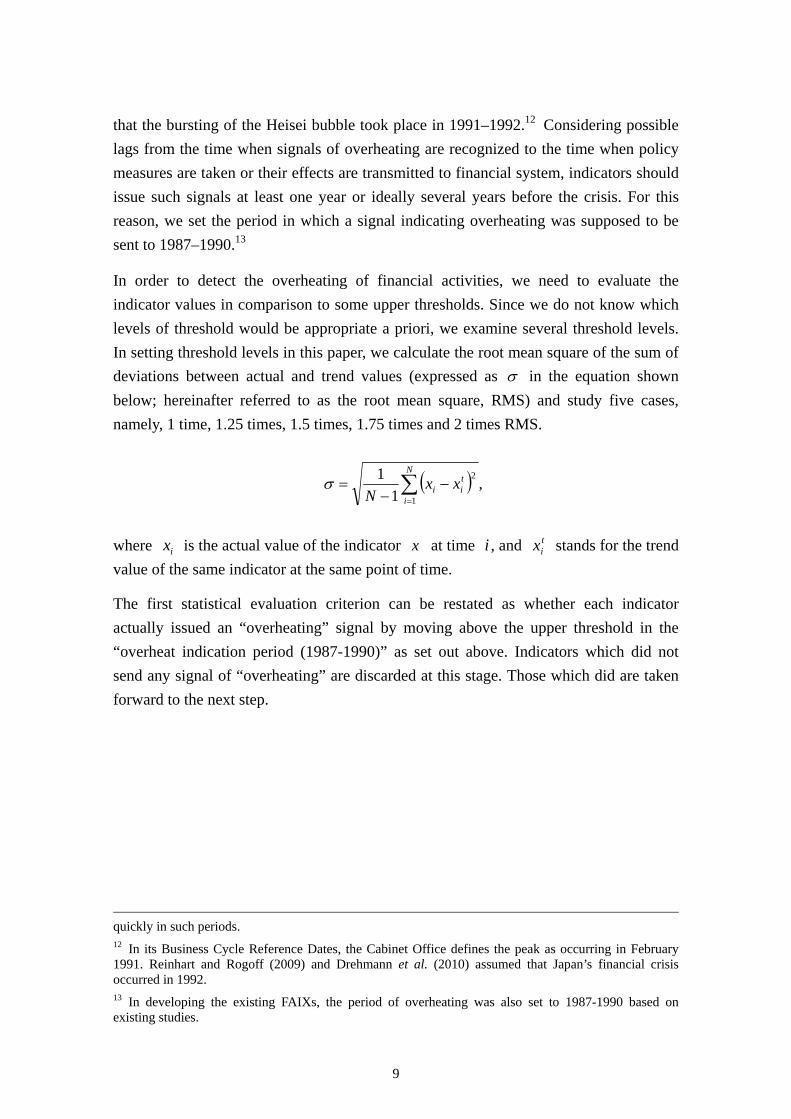
In setting threshold levels in this paper, we calculate the root mean square of the sum of

deviations between actual and trend values (expressed as in the equation shown

below; hereinafter referred to as the root mean square, RMS) and study five cases,

namely, 1 time, 1.25 times, 1.5 times, 1.75 times and 2 times RMS.

,1

1

1

2

N

i

tii xx

N

where ix is the actual value of the indicator x at time i , and tix stands for the trend

value of the same indicator at the same point of time.

The first statistical evaluation criterion can be restated as whether each indicator

actually issued an “overheating” signal by moving above the upper threshold in the

“overheat indication period (1987-1990)” as set out above. Indicators which did not

send any signal of “overheating” are discarded at this stage. Those which did are taken

forward to the next step.

quickly in such periods. 12 In its Business Cycle Reference Dates, the Cabinet Office defines the peak as occurring in February 1991. Reinhart and Rogoff (2009) and Drehmann et al. (2010) assumed that Japan’s financial crisis occurred in 1992. 13 In developing the existing FAIXs, the period of overheating was also set to 1987-1990 based on existing studies.

10

(ii) Statistical evaluation II: Evaluating statistical errors

When using indicators to make a financial activity assessment, it is ideal that warning

signals be issued before an event, i.e., a financial crisis, takes place, and that no warning

signals are dispatched when no such event is occurring. It is desirable that either A or D

in the table below always be realized:

Event No event

Signal issued Correct signal: A Type II errors: B

No signal issued Type I errors: C Correct signal: D

Indicators, however, do not always send appropriate signals, and the occurrence of

events and signals thereof could involve two types of errors. The first type, or “type I

errors,” is a case in which indicators fail to issue any signals of an event that is actually

occurring. In the above table, C falls under this category, which can be described as a

“risk of missing crises.” In the second type, or “type II errors,” indicators issue crisis

signals despite no such event arising, to which the case of B in the above table

corresponds. This represents a “risk of issuing false signals.”

The threshold should be set at a relatively low level if one would like to to minimize the

occurrence of “type I errors (= risk of missing crises)” so that signals are issued at a

reasonably early stage. This will allow as many crisis signals as possible to be sent so

that no crisis is overlooked as it occurs. Meanwhile, there is also a need to keep

thresholds at a relatively high level to lower the frequency with which false signals are

issued, thereby reducing “type II errors (= risk of issuing false signals).” Thus, trying to

reduce “type I errors” will cause thresholds to be on the low side, and trying to reduce

“type II errors” will cause thresholds to be on the high side. There is a trade-off between

these two objectives (Figure 6).

In this paper, the period for which “type I errors” and “type II errors” are examined is

1980-2005, with the period from 2006 onward not being included in statistical

verification. This is because there is not necessarily consensus as to the appropriateness

of assuming the pre-Lehman shock period represents an overheating phase of financial

activity in Japan.

In the literature, several statistical models are perceived as useful in evaluating

indicators. Here we perform statistical evaluation using four such models as explained

below. If the majority of the models select an indicator, that is taken as the best choice.

If more than one indicator in the same category survives the statistical verification

11

process, a single indicator is ultimately selected based on a judgmental assessment.

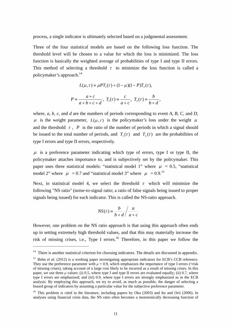
Three of the four statistical models are based on the following loss function. The

threshold level will be chosen to a value for which the loss is minimized. The loss

function is basically the weighted average of probabilities of type I and type II errors.

This method of selecting a threshold to minimize the loss function is called a

policymaker’s approach.14

),()1)(1()(),( 21 TPPTL

,)(,)(, 21 db

bT

ca

cT

dcba

caP

where, a, b, c, and d are the numbers of periods corresponding to event A, B, C, and D,

is the weight parameter, ),( L is the policymaker’s loss under the weight

and the threshold , P is the ratio of the number of periods in which a signal should

be issued to the total number of periods, and )(1 T and )(2 T are the probabilities of

type I errors and type II errors, respectively.

is a preference parameter indicating which type of errors, type I or type II, the

policymaker attaches importance to, and is subjectively set by the policymaker. This

paper uses three statistical models: “statistical model 1” where = 0.5, “statistical

model 2” where = 0.7 and “statistical model 3” where = 0.9.15

Next, in statistical model 4, we select the threshold which will minimize the

following "NS ratio" (noise-to-signal ratio; a ratio of false signals being issued to proper

signals being issued) for each indicator. This is called the NS-ratio approach.

ca

a

db

bNS

)(

However, one problem on the NS ratio approach is that using this approach often ends

up in setting extremely high threshold values, and that this may materially increase the

risk of missing crises, i.e., Type I errors.16 Therefore, in this paper we follow the 14 There is another statistical criterion for choosing indicators. The details are discussed in appendix. 15 Behn et al. (2012) is a working paper investigating appropriate indicators for ECB’s CCB reference. They use the preference parameter with μ = 0.9, which emphasizes the importance of type I errors (=risk of missing crises), taking account of a large cost likely to be incurred as a result of missing crises. In this paper, we use three μ values: (i) 0.5, where type I and type II errors are evaluated equally; (ii) 0.7, where type I errors are emphasized; and (iii) 0.9, where type I errors are strongly emphasized as in the ECB analysis. By employing this approach, we try to avoid, as much as possible, the danger of selecting a biased group of indicators by assuming a particular value for the subjective preference parameter. 16 This problem is cited in the literature, including papers by Oka (2003) and Ito and Orii (2006). In analyses using financial crisis data, the NS ratio often becomes a monotonically decreasing function of

12

“modified noise-to-signal ratio approach” adopted by Drehmann et al. (2010).

Specifically, we focus solely on indicators which issue signals in more than two-thirds

of the overheat indication period. We then select one of these indicators which has the

lowest NS-ratio.

Having discussed the indicator selection process, let us now explain how the above

process is implemented in practice in terms of specific indicators. As an example, we

look at indicators which represent funding activity in the private sector. We first use

statistical model 1, then choose the total credit to GDP ratio as the first candidate

indicator. The loss function values of this indicator in each combination of the two trend

types (the 3-year backward moving average and the one-sided HP filter) and the five

thresholds (1 time, 1.25 times, 1.5 times, 1.75 times and 2 times RMS), i.e., 10

combinations in all, are then calculated. From these calculation results, the lowest loss

function value and the relevant trend extraction method and threshold are then recorded.

The year-on-year growth rate of total credit is then taken as the second candidate

indicator. Again, the loss function values in all the combinations of the two trend types

and the five thresholds are calculated, and the lowest loss function value and the

relevant trend extraction method and threshold are recorded. The same calculations are

performed for all other indicators in the same category. The indicator with the smallest

loss function value (and the relevant trend extraction method and threshold) is selected

as the optimal indicator in statistical model 1 for that particular category. The same

process is repeated for statistical models 2, 3 and 4, with the optimal indicator being

selected for each of them. The indicator (and the relevant trend extraction method and

threshold) selected by the majority of the four models is the best indicator for the

category in question.

(2) Selection results

The selection results are shown in Figure 7. For each category, the indicators selected by

the four statistical models are shown with the trend extraction methods and thresholds.

For example, in the category of financial institutions and investment activity, two out of

four models choose DI of lending attitudes of financial institutions with trend of past

average and threshold of one time RMS. One model chooses ROA from net interest

income of banks with trend of one-sided HP filter and threshold of one time RMS. No

indicators are chosen for the last statistical model. Since two out of the four models

choose DI of lending attitudes of financial institutions, the indicator (and the relevant the threshold (τ) in an appropriate range, and the optimal interior solution cannot be obtained in many such cases. For this reason, the policymaker’s approach has been adopted in some recent analyses. See, for example, Babecky et al. (2012) and Sarlin (2013).

13

trend extraction method and threshold mentioned above) is the best for this category. In

the category of private sector and funding activity, all the models choose total credit to

GDP ratio. Two out of the four models choose the indicator with trend of one-sided HP

filter and threshold of one time RMS, one with trend of 3-year moving average and

threshold of 1.25 times RMS, and one with trend of 3-year moving average and

threshold of one time RMS. Therefore, total credit to GDP ratio with trend of one-sided

HP filter and threshold of one time RMS is selected as the best in this category. Same

procedure is applied for other categories and the best indicators are chosen.

The selected 14 indicators are shown in Figure 8.

3. Characteristics of each indicator

In the manner described above, we examined 321 variables, using different trend

extraction methods, and we choose optimal indicators based on two statistical criteria:

(a) whether the variables issue signals of the overheating of the Heisei bubble, and (b)

whether statistical errors are minimized. As a result, two of the 10 previously selected

indicators were abandoned, one was retained, three were retained with different trend

extraction methods, four with different processing methods applying to the original data

series, and six new indicators were added (Figure 8). Thus, the number of indicators

comprising FAIXs was increased from 10 to 14 by the revision. More than one indicator

was left as a candidate in the category of land prices and that of corporate investment

activity. The selections of indicators in these categories are discussed in detail in the

following section.

We now summarize the characteristics of the indicators selected above, classifying them

into five groups: (1) indicators to be abandoned; (2) an indicator to be retained and used

in the same way; (3) indicators to be retained with different trend extraction methods;

(4) indicators to be retained with different processing methods applying to the original

data series; and (5) newly adopted indicators.

(1) Indicators to be abandoned

(i) Ratio of firms’ CP outstanding to their liabilities

In periods leading to financial crises in overseas economies, firms have tended to

become more reliant on financing from short-term funding markets in an effort to

increase their assets to expand their business (Minsky, 1982). The ratio of firms’ CP

outstanding to their liabilities was chosen as one of the indicators in FAIXs, as in

addition to such overseas cases, its actual value immediately before the Lehman shock

14

indicated a move toward overheating (Figure 9). This indicator, however, has contain

following problems. First, because no data are available for the Heisei bubble period, no

back-testing can be done to establish whether it issued appropriate signals before the

crisis in Japan. Second, it did indicate an overheating tendency before the Lehman

shock, but it continued to do so up to around the early 2009, i.e., in the post-Lehman

shock period as well. In particular, we need to take account of the fact that firms

actively issued CP immediately after the Lehman shock to secure their on-hand liquidity,

and that this can hardly be interpreted as an overheating of financial activity.

Consequently, we believe it is appropriate to exclude this indicator from FAIXs.

(ii) Spread between expected equity yields and government bond yields

The spread between expected equity yields and government bond yields is the

difference between expected earnings per share divided by the share price and the

long-term interest rate, as shown in Equation (1). From this equation, and based on the

share price determining equation shown in Equation (2), the spread between expected

equity yields and government bond yields is equivalent to the risk premium for equity

investment less the growth rate of expected earnings per share, as shown in Equation

(3).

i

P

Eyields bond government and yieldsequity expectedbetween Spread

(1)

RPgi

EP

）（price Share

(2)

gRPi

P

Eyields bond government and yieldsequity expectedbetween Spread

(3)

Here, P is the share price, E is expected earnings per share, i is the long-term interest

rate, g is the growth rate of expected earnings per share and RP is the risk premium.

It is apparent that this indicator trended upward from the early-1990s (Figure 10). Based

on the above equation (3), this can be interpreted as indicating the growth rate of

expected earnings per share (g) trended downward. Cyclical changes around such a

trend can be described as showing the short-term cyclical fluctuations in the risk

premium and the growth rate of expected earnings per share.

Since the starting period of the sample of this indicator is the first quarter of 1991, we

cannot implement statistical examination for signals of the overheating of the Heisei

bubble. Therefore, we decided to abandon this indicator.17

17 We examined spread between actual equity yields and government bond yields, which uses actual, not expected earnings per share. That indictor was included in the category of stock price. As a result of the statistical examination, this indicator was not chosen.

15

(2) Indicator to be retained and used in the same way

The indicator which will be retained and used, applying the same calculation method

and threshold, is “equity weighting in institutional investors’ portfolios.” This was

selected as the best indicator in the category of investment activity in the financial

market. We examined other indicators, such as those relating to the investment activities

of overseas investors and various interest rates. However, we selected this indicator,

inheriting from the existing index, on the basis of its statistical usefulness. This

indicator signaled overheating in most of the Heisei bubble period, and thus can be

expected to capture investment activity in stock markets well (Figure 11).

(3) Indicators with different trend extraction methods

(i) DI of lending attitudes of financial institutions

In the existing FAIXs, the 3-year backward moving average was used as a trend

extraction method, and deviations of actual indicator values from the trend were used as

gap values of the indicator. As a result of the current examination, the gap indicator is

now calculated using the past average as the trend. The threshold is one time RMS. In

the Heisei bubble period, the actual values of this indicator did not signal “overheating”

despite its high level, because the trend closely followed movements in the actual values

of the indicator (Figure 12(1)). In contrast, the new indicator based on the past average

has signaled overheating in the same period (Figure 12(2)). Financial institutions’

lending attitude is a statistic which should be considered to have a mean-reverting

nature, as the lending attitude is not supposed to fluctuate much in the long run. The

current investigation resulted in selecting a gap indicator of this nature.

(ii) Total Credit to GDP ratio

In the existing FAIXs, past 3-year moving averages were calculated as trends, and

deviations of actual values from these trends were used as gap values of indicators. This

was also the case with the total credit to GDP ratio. In the current examination, in

addition to the existing method, we examined another way to extract trends, i.e., the

one-sided HP filter, which is an approach adopted by the BCBS in its guidance for CCB

decisions, and other data processing methods (such as year-on-year growth rate and

deflating nominal data to real values) as well. As a result, we adopted the total credit to

GDP ratio with a trend extracted by the one-sided HP filter, which is used in the BCBS

guidance.18 The threshold is one time RMS. No major differences were observed for

18 We also examined the performance of DSR (Debt Service Ratio), which is one of the useful indicators to capture the private funding activity. However, the results supported the adoption of the total credit to

16

both indicators, and the differences in the judgments concerning overheating or

overcooling between the existing and new indicators were minimal. In terms of

minimizing statistical errors, however, the current indicator demonstrated better results

(Figure 13).

(iii) Stock prices

As the indicator for stock prices, the existing FAIXs adopted an indicator of the

deviation of actual stock prices (TOPIX) from their 3-year backward moving average.

In the current examination, we examined several additional candidate indicators,

including stock price normalized by GDP and the spread between actual equity yields

and government bond yields, and examined a method of extracting trends using the

one-sided HP filter. Based on the statistical examination, we again selected stock prices

(TOPIX) as a variable, but chose the one-sided HP filter as a trend extraction method

and a threshold of 1.5 times RMS (Figure 14). The new threshold value chosen on the

basis of minimizing statistical errors is larger than that of the existing indicator.

(4) Indicators to be retained with different processing methods applying to the original data series

(i) Money multiplier (ratio of M2 to the monetary base) and M2

Early studies demonstrated that the money multiplier was a variable indicating financial

intermediation activity by financial institutions (Kaminsky and Reinhart, 1999). In

comparison with monetary base representing fundamental economic liquidity, the

amount of money (M2) increases significantly when credit creation by financial

institutions becomes active as they extend loans aggressively.

The money multiplier was also included in the candidate indicators of the current

examination. As a result of the statistical examination, however, we chose the M2

growth rate, with the trend extracted using the one-sided HP filter and the threshold of

one time RMS. The actual movement of the M2 growth rate indicates overheating in the

Heisei bubble period and overcooling in the subsequent period (Figure 15).

In addition to its statistical inferiority, another problem with the money multiplier is that

its nature can change depending on what kind of monetary policy measures are

implemented. When a central bank shifts its policy focus from traditional short-term

interest rate operations to non-traditional base money operations such as quantitative

easing, the nature of monetary base changes from being an endogenous variable to an

GDP ratio. We are grateful to Mr. Mathias Drehmann of BIS for kindly providing the data of DSR for the examination.

17

exogenous variable (or, a "policy variable"). For example, in Japan, monetary base

increased significantly and as a result the money multiplier decreased substantially

when quantitative easing or quantitative and qualitative monetary easing has been

implemented (Figure 15). However, such a large decrease in the money multiplier does

not mean that the financial intermediation and credit creation of financial institutions

contracted materially at that time.

(ii) Land prices

In the existing FIAXs, a gross rent multiplier (= ratio of land prices to rent; land prices

are all use categories in the Tokyo area) was used as an indicator for land prices. In this

examination, we also included land prices normalized by GDP or other income-related

variables or deflated by the consumer price index, in the candidate indicators. At the

same time, we examined land prices not only in the Tokyo area, but also in six major

cities (including the Tokyo area) and land price variables for different use categories,

such as commercial and residential.

As a result of the statistical examination, several indicators were selected in each

statistical model category: the land price to GDP ratio (land price of six major cities/all

use categories average); the real land prices (land price of six major cities/all use

categories average); and the real land prices (land price of six major cities/commercial

use category).19 We choose the land prices to GDP ratio (land price of six major

cities/all use categories average) based on the following judgments: first, it covers a

wide range of land usages and cities; and second, it is normalized by the size of

economy. The trend is calculated using the 3-year backward moving average, and the

threshold is one time RMS. It was found that both the existing and newly selected

indicators issued an overheating signal in the Heisei bubble period in a similar manner,

and that their movements in other periods were also nearly identical (Figure 16).

(iii) Business fixed investment to GDP ratio

The index representing firms’ investment activity used in the existing FAIXs is the ratio

of firms’ investments to operating profits, where firms’ investments comprise fixed

investments, inventory investments and security investments (Figure 17(1)). In the

current examination, we also investigated other definitions for the numerator, such as

firms’ investments excluding security investments, which are largely influenced by

stock price fluctuations, or fixed investments alone. We also investigated the case with

GDP as a denominator variable.

19 The 'real' variables are deflated by the Consumer Price Index.

18

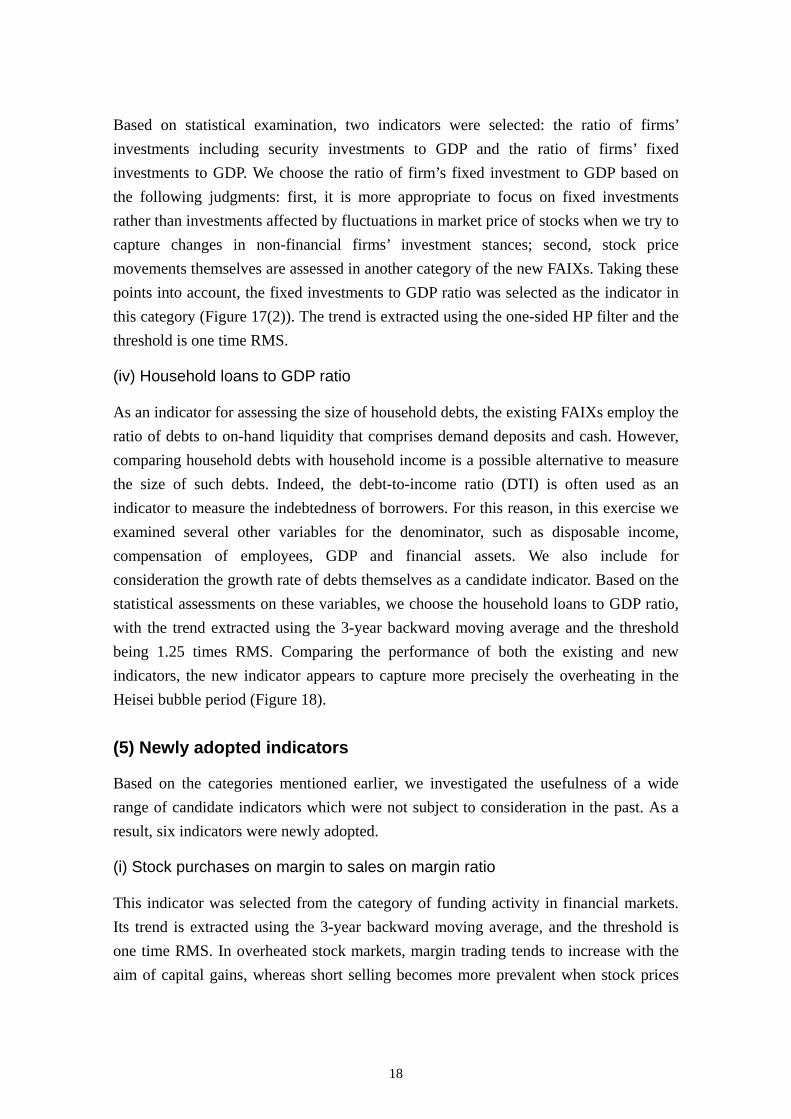
Based on statistical examination, two indicators were selected: the ratio of firms’

investments including security investments to GDP and the ratio of firms’ fixed

investments to GDP. We choose the ratio of firm’s fixed investment to GDP based on

the following judgments: first, it is more appropriate to focus on fixed investments

rather than investments affected by fluctuations in market price of stocks when we try to

capture changes in non-financial firms’ investment stances; second, stock price

movements themselves are assessed in another category of the new FAIXs. Taking these

points into account, the fixed investments to GDP ratio was selected as the indicator in

this category (Figure 17(2)). The trend is extracted using the one-sided HP filter and the

threshold is one time RMS.

(iv) Household loans to GDP ratio

As an indicator for assessing the size of household debts, the existing FAIXs employ the

ratio of debts to on-hand liquidity that comprises demand deposits and cash. However,

comparing household debts with household income is a possible alternative to measure

the size of such debts. Indeed, the debt-to-income ratio (DTI) is often used as an

indicator to measure the indebtedness of borrowers. For this reason, in this exercise we

examined several other variables for the denominator, such as disposable income,

compensation of employees, GDP and financial assets. We also include for

consideration the growth rate of debts themselves as a candidate indicator. Based on the

statistical assessments on these variables, we choose the household loans to GDP ratio,

with the trend extracted using the 3-year backward moving average and the threshold

being 1.25 times RMS. Comparing the performance of both the existing and new

indicators, the new indicator appears to capture more precisely the overheating in the

Heisei bubble period (Figure 18).

(5) Newly adopted indicators

Based on the categories mentioned earlier, we investigated the usefulness of a wide

range of candidate indicators which were not subject to consideration in the past. As a

result, six indicators were newly adopted.

(i) Stock purchases on margin to sales on margin ratio

This indicator was selected from the category of funding activity in financial markets.

Its trend is extracted using the 3-year backward moving average, and the threshold is

one time RMS. In overheated stock markets, margin trading tends to increase with the

aim of capital gains, whereas short selling becomes more prevalent when stock prices

19

trend downward.20 Against this backdrop, we included the ratio of stock purchases on

margin to sales on margin in the candidate indicators. This indicator shows overheating

in the Heisei bubble period (Figure 19), as well as around 2000, when the so-called IT

bubble took place.

(ii) Private investment to GDP ratio

This indicator was selected from the category of investment activity in the private

non-financial sector (households and businesses). Private investment includes firms’

fixed and inventory investments and households’ housing investments and consumer

durables expenditure.21 The trend is extracted using the 3-year backward moving

average, and the threshold is one time RMS. Financial institutions adopt a more relaxed

lending attitude when financial activity is overheating, and then financing becomes

easier for entities in the private non-financial sector, such as businesses and households.

Moreover, financial overheating tends to encourage optimistic expectations of future

profits and incomes, which then accelerate corporate and household investment

activities. It is the private investment to GDP ratio that captures these tendencies. It

indicates an overheating of financial activity in the Heisei bubble period (Figure 20). In

addition to the above comprehensive definition, we investigated other candidates for the

ratio’s numerator, i.e., other types of investment, such as security investments and fixed

capital investments (the sum of fixed investments and housing investments). However,

the private investment to GDP ratio was selected as a result of statistical examination.

(iii) Household investment to disposable income ratio

This indicator was selected from the category of investment activity of household.

Household investments include housing investments and consumer durable goods

consumptions. The indicator’s trend is extracted using the 3-year backward moving

average, and the threshold is one time RMS. As mentioned earlier, household

investment activity tends to be accelerated by lax lending attitudes among financial

institutions, and optimistic assumptions regarding future incomes fostered during a

financial boom. This indicator captures this tendency, and it issued an overheating

signal in the Heisei bubble period (Figure 21). Other candidates considered include

housing investments, security investments and financial assets. We also investigated

other variables including GDP as the denominator. The household investment to

disposable income ratio was ultimately selected based on statistical examination.

20 Galbraith (1990) points out that margin trading was actively conducted in the uptrend in stock markets in the U.S. prior to the Great Depression. 21 We do not include investments in lands due to data availability.

20

(iv) Corporate credit to GDP ratio

This indicator was chosen from the category of funding activity of corporate sector. The

trend is extracted using the 3-year backward moving average, and the threshold is one

time RMS. In an overheating phase of financial activity, businesses tend to accelerate

their investment activity and to rely on borrowings to fund their investments, prompted

by a relaxed lending attitude among financial institutions and optimistic expectations of

future profits. Authorities in a increasing number of countries monitor the state of

business credit, and some of them are examining this variable as one of the reference

indicators for CCB decisions. This indicator issued a signal indicating overheating in

the Heisei bubble period (Figure 22). In this category, we also investigated several other

indicators such as corporate credit growth rate, corporate credit to GDP ratio, and

changes in corporate credit to GDP ratio. In addition, possibilities of using operating

profits or on-hand liquidity are explored in this examination.

(v) Real estate firm investment to GDP ratio

This indicator was selected from the category of investment activity of real estate sector.

The real estate firms’ investments include fixed investments, land investments and

inventory investments. The trend is extracted using the one-sided HP filter, and the

threshold is one time RMS. In real estate booms, realty firms tend to engage themselves

in active developments of commercial facilities and office buildings, thereby increasing

their real asset investments. Accordingly, a shift in realty firms’ investments can be an

early warning indicator. Indeed in Japan, this indicator sent a signal suggesting a certain

level of overheating in the Heisei bubble period around the latter half of 1980s (Figure

23). Similarly, it issued a signal implying overheating in realty firms’ investments in

around the mid of the 2000s, when a real estate boom by newly established realty firms

was said to be emerging. We investigated different numerators such as a combination of

realty firms’ real investments and their security investments, and different denominators

including sales and operating profits in addition to GDP.

(vi) Real estate loans to GDP ratio

This indicator was selected from the category of funding activity of real estate sector.

The trend is extracted using the one-sided HP filter, and the threshold is one time RMS.

Overheating of the real estate sector has been a source of financial crises in bubble

episodes experienced in a number of countries (Galbraith, 1990; Kindleberger, 2000).

Similarly, one phenomenon observed in the Japan’s Heisei bubble was that real estate

firms’ outstanding loans increased substantially as real estate prices rose. There are two

reasons for this: first, when speculative real estate transactions become common, driven

21

by price increase in real estate, firms’ funding requirements for such deals increase; and

second, because real estate serves as collateral for loans, the limits for such loans will be

raised as their collateral value rises along with an increase in its price. Kiyotaki and

Moore (1997) found that changes in the volume of credit due to variations in values of

collateralized real estate have a major impact on economic fluctuations, and named this

phenomenon the “credit cycle.” Thus, loans to real estate firms tend to increase

substantially when financial activity becomes overheated. Tracing movements in the

level of loans to real estate firms in Japan, it is indeed obvious that a signal indicating a

overheating started to be issued in the mid of the 1980s and continued to be sent until

early 1990s, i.e., just before the collapse of the bubble economy (Figure 24). In addition

to loans to real estate firms, we examined total debts including funds raised in the

market as the numerator variable. Furthermore, real estate firms’ operating profits were

examined as a denominator variable.

4. New heat map

Based on the above examination, we abandon two indicators, retain one, revise three

with different trend extraction methods, revise four with different processing methods

applying to the original data series, and adopt six new indicators. Therefore, the new

FAIXs consist of 14 indicators. A new heat map based on the new configuration of

indicators is shown in Figure 25. Compared with the existing FAIXs, while both

versions exhibit the same feature of indicating overheating during the Heisei bubble

period, the new version contains a larger number of indicators which issue signals

suggesting overheating of the bubble. The episode available for testing performance of

the indicators in detecting a bubble is basically limited to the Heisei bubble. Despite this

limitation, however, we believe that the upgraded and expanded FAIXs will be more

useful from the perspective of closely monitoring early warning indicators in order to

avoid emergence of the same type of bubbles as the Heisei bubble, which have a major

negative impact on financial activity and the real economy in Japan.

Verifying the new index’s performance just prior to the Lehman shock, which is not a

part of the statistical examination described in the previous sections, the indicator for

real estate firms’ investment alone indicates overheating. At that time, active real estate

investments in urban areas were observed in Japan, and several bankruptcies of young

real estate firms were filed in the post-Lehman shock economic downturn. Nevertheless,

the situation did not develop into a major episode of financial system turmoil. We

consider that the new FAIXs correctly capture such situations, and that this supports the

usefulness of the new index, while acknowledging that much implication cannot be

22

drawn from this one episode.

Two indicators, namely, the household loans to GDP ratio and the corporate credit to

GDP ratio, indicated overheating immediately after the Lehman shock. This is due to a

substantial drop in GDP, the denominator, within a short period of time after the

Lehman shock. Thus, an unusual move in a denominator variable can cause major

fluctuations in the ratio, which can trigger a signal. The BCBS’s CCB guidance points

to the risk that such a move may cause the credit to GDP ratio indicator to issue an

overheating signal in a serious economic downswing period (BCBS, 2010). Thus there

is a need to carefully observe the denominator variables themselves as well when

making judgments on the movement of indicators normalized by variables such as GDP.

A comparison of the new and old heat maps shows that the “stock purchase on margin

to sales on margin ratio” in the new heat map indicates an overheating of financial

activity. In contrast, “stock prices” in the existing heat map do so. The “stock price”

indicator is adopted in both versions. However, a higher threshold value has been set for

this indicator in the new index based on the statistical examination, and as a result no

indication of overheating is issued in the new heat map.

5. Summary and points to be noted

(1) Summary

This paper discusses the revision of FAIXs taking into account recent analyses of early

warning indicators and examples of reference guides for the CCB in other countries.

Prior to carrying out the selection process, indicators were divided into two categories --

indicators representing investment activity and those representing funding activity -- for

each type of economic agent, such as financial institutions and businesses. In addition,

asset prices were sorted into two categories: stock prices and land prices. 14 indicator

categories were then established in all. In the course of selecting a single indicator for

each category, we examined the usefulness of individual indicators from the two

perspectives: (a) whether they can capture the overheating of the Heisei bubble period,

which had a major impact on economic and financial activities in Japan, and (b)

whether statistical errors of various types can be minimized. We also used various trend

extraction methods and several threshold values. As a result of these examinations, two

of the 10 indicators comprising the existing FAIXs are abandoned, one is retained, three

are revised with different trend extraction methods, and four with different processing

methods applying to the original data series. The 14 indicators, including these eight

and the newly chosen six, now constitute the new FAIXs.

23

(2) Points to be noted

The following points need to be noted when analyzing financial activity situations using

the new FAIXs.

First, it is important to have comprehensive judgments on financial conditions.22 It

would be convenient if we could make a judgment on financial conditions totally based

on a limited number of indicators. However, we need sufficient lengths of time series

data in order to construct early warning system based on the past overheating and

overcooling episodes of financial activities. 23 When financial activities become

overheated, newly developed financial transactions and products can emerge in order to

avoid existing regulations. In this case, it is difficult to capture such a movement by

using existing statistics. We saw such an example of “shadow banking activities” in the

recent global financial crisis. As such, we may run a risk to overlook newly developed

financial imbalances if we only concentrate on the existing statistics. While it is

important to upgrade statistical analysis, we need to make efforts to capture any newly

developed potential risks by acquiring various information regarding financial

institutions’ activities and financial market developments. In this regard, information on

financial institutions’ activities obtained through on site examinations and off site

monitoring/hearing is very useful when we assess “financial overheating and

overcooling.”24 Some changes in risk-taking attitudes among financial institutions are

likely to threaten the stability of the financial system in future. Such changes may not be

reflected in macro statistics, but may be clarified through direct contact with financial

institutions, such as hearings. Thus, there is a need to make comprehensive judgments

on financial system situations based on a wide range of information, including those

items mentioned above.

Second, we need to remain vigilant over interactions of various sorts. The indicators

analyzed in this paper basically focus on individual economic agents and the market

developments which these indicators respectively cover. However, the recent global

financial crisis has demonstrated the need to gain a precise understanding of the

22 The CCB guidance by BCBS (2010) also emphasized importance of judgment for the assessment of financial conditions. 23 In this paper, we only investigate indicators available in the past providing signals of the overheating in the Heisei bubble period. It is possible that newly available data be useful indicators to detect the overheating of the bubble economy at early stage in future. 24 Financial System Report of the Bank of Japan comprehensively assesses the state of financial intermediation and risks in financial system in Japan. In the process of the assessment, we rely on qualitative information obtained through on site examinations and off site monitoring/hearing as well as quantitative results of our analyses on a number of types of risks borne by Japanese financial institutions.

24

interrelationships at play between key factors in a financial crisis, such as feedback loop

between financial sector and the real economy, transaction relations between financial

institutions, and the status of various risk transfers. For this reason, other approaches

have also started to be taken by authorities in many countries: macro stress testing,

which takes account of a variety of interactions, and risk monitoring, which utilizes

financial institutions’ transaction data.25 It is necessary to continue conducting studies

in this field, including the adoption of these new analytical methods, so that any kind of

risks which may emerge in the future can be dealt with as effectively as possible.

Third, we need to be mindful of the significance attached to trend values. Our concern

in the current analysis has been whether a “gap indicator,” which captures deviations of

actual values from trend values, has issued appropriate signals in an episode of financial

activity overheating, and whether associated statistical errors have been minimized. A

trend value itself, therefore, is not given the meaning of “an equilibrium value which

would have been realized had it not been for a bubble or a financial imbalance.” Indeed,

land price movements demonstrate this point: actual land prices, which rose

significantly in the Heisei bubble period, largely declined after the bubble, and their

trend values also display similar fluctuations with some time lags (Figure 16). This

clearly indicates that trend values in the bubble period cannot be interpreted as showing

“had-it-not-been-for-a-bubble levels.” How asset prices or credit volumes deviate from

a “level which should have occurred” in an episode of financial overheating is a subject

that must be analyzed separately using tools such as theoretical models.

25 Financial System Report of the Bank of Japan assesses the resilience of Japan's financial system against macro risks by conducting macro stress testing using the Financial Macro-econometric Model, which models the interrelationship between the financial system and the real economy. In the testing, we quantitatively analyze the effects on the financial system of a significant economic downturn and a substantial rise in interest rates.

25

Appendix: Statistical criterion for choosing indicators

In this appendix, we explain a statistical criterion for choosing indicators which has

been used recently. That is receiver operating characteristics curve (ROC curve).26

1. ROC curve

ROC curve is the relationship between the rate of “true positive” and that of “false

positive” for different values of the threshold. The rate of true positive is the probability

of dispatching correct signals when event occurs (i.e., 1 minus probability of type I

errors). The rate of false positive is the probability of dispatching false signals when no

event occurs (i.e., probability of type II errors). If the threshold is set at a lower level,

more signals tend to be dispatched and events are easily signaled. However, in that case,

there is a high risk of type II error. If the threshold is set at a higher level, fewer signals

are dispatched and events are not easily signaled. In that case, risk of type II error is low.

Therefore, there is a positive relationship between the rates of true positive and false

positive. Three typical forms of ROC curve are depicted in Figure 26.

First, suppose that an indicator is perfect in the sense that, with the optimal threshold, it

can signal future events accurately without type II error. The ROC curve in this case is

depicted in Figure 26(1). The upper-left point (0,1) corresponds to the outcome with the

optimal threshold. If the threshold is lowered from the optimal level, the true positive

rate decreases while the false positive rate does not change from zero. Thus the point

corresponding to the outcome moves downwards on the vertical part of the curve. On

contrary, if the threshold is raised from the optimal level, the false positive rate

increases while the true positive rate does not change from one. Therefore, the

corresponding point moves in the right direction on the horizontal part of the curve.

Next, consider an indicator which is completely uninformative (Figure 26(2)). For

example, starting from the origin (which corresponds to the outcome with an extremely

high threshold), if the threshold is lowered, the rates of true positive and false positive

increase by the same amount. Therefore, the point corresponding to the outcome moves

in the upper-right direction on the ROC curve, which is, in this case, a straight line with

an angle of 45 degrees. In this case, we have signals, but prediction power of the

indicator is 'fifty-fifty' under any value of thresholds. That is, using the indicator is

equivalent to tossing a coin, and in this sense, the indicator contains no information.

26 This analysis is originally from studies of radar where characteristics of radar signal receivers were examined.

26

Most of indicators to be used for early warning system are those between the above

extreme cases. A typical ROC curve is shown in Figure 26(3). In this case, starting from

the origin, if the threshold is lowered, the true positive rate increases more than the false

positive rate does. Thus the point corresponding to the outcome moves in the

upper-right direction on the curve, which is located above the 45-degree line. In this

case, if the threshold is set at an appropriate level, the indicator can correctly predict

events with a probability higher than 50%. Therefore, using the indicator is better than

tossing a coin.

2. Relationship between the policy makers’ approach and ROC curve

The curve in Figure 26(3) is ROC curve, the relationship between the rates of true

positive and false positive for different values of the threshold. The policymakers will

decide which point of ROC curve is optimal with the corresponding threshold when

they use indicators for anticipation of a future event. If policymakers attach more

attention to the risk they overlook the event, they would like to have lower threshold

levels and capture the event as much as possible. In this case, however, they need to

accept higher incidents of type II errors. This situation is point A in Figure 27(1). If

policymakers have tendency to avoid type II error, they will set higher threshold levels.

This situation is point B in Figure 27(1).

The policymakers’ approach we employ in this paper for choosing appropriate

indicators and thresholds is equivalent to ROC curve approach with optimal

combination of true positive and false positive (Figure 27(2)). In the main text, we

examined the usefulness of indicators directly calculating values of loss functions,

taking into account various combinations of preference parameters.27

3. Example of ROC curve

We show an example of ROC curve using an indicator we used in the main text. 2 cases

for the total credit to GDP ratio are depicted in Figure 27(3), one with one-sided HP

filter trend case and the other with 3-year backward moving average. Both curves are

positioned above 45 degree line and thought to be useful indicators. Comparing these

two, one with one-sided HP filter trend is positioned higher and thought to be a better

indicator.

27 In addition, there is the analytical method for measuring the area under ROC. Drehmann (2014) points out that the credit to GDP ratio is the best indicator according to this criterion.

27

References

Adrian, Tobias, Daniel Covitz, and Nellie Liang, 2013. “Financial Stability Monitoring.”

Finance and Economics Discussion Series, 2013-21, Board of Governors of the

Federal Reserve System.

Babecky, Jan, Tomas Havranek, Jakub Mateju, Marek Rusnak, Katerina Smidkova, and

Borek Vasicek., 2012. “Banking, debt and currency crisis: Early warning indicators

for developed countries.” ECB Working Paper No. 1485.

Bank of England, 2014. “The Financial Policy Committee’s Powers to Supplement

Capital Requirements.” A Policy Statement.

Basel Committee on Banking Supervision, 2010. “Guidance for National Authorities

Operating the Countercyclical Capital Buffer.” Bank for International Settlements.

Behn, M., C. Detken, T. A. Peltonen, and W. Schudel, 2013. “Setting Countercyclical

Capital Buffers Based on Early Warning Models: Would it Work?” ECB Working

Paper No 1604.

Borio, Claudio, Mathias Drehmann, 2009. “Assessing the Risk of Banking Crises –

Revisited.” BIS Quarterly Review, March 2009.

Borio, Claudio, and Philip Lowe, 2002. “Assessing the Risk of Banking Crises.” BIS

Quarterly Review, December 2002.

Drehmann, Mathias, Claudio Borio, Leonardo Gambacorta, Gabriel Jimenez, and

Carlos Trucharte, 2010. “Countercyclical Capital Buffers: Exploring Options.” BIS

Working Papers, No 317.

Drehmann, Mathias, Claudio Borio, and Kostas Tsatsaronis, 2011. “Anchoring

Countercyclical Capital Buffers: The Role of Credit Aggregates.” BIS Working

Papers, No. 355.

Drehmann, Mathias, and Mikael Juselius, 2012. “Do debt service costs affect

macroeconomic and financial stability?” BIS Quarterly Review, September 2012.

Drehmann, Mathias, and Kostas Tsatsaronis, 2014. “The Credit-to-GDP Gap and

Countercyclical Capital Buffers: Questions and Answers.” BIS Quarterly Review,

March 2014.

Galbraith, John Kenneth, 1990. A Short History of Financial Euphoria. Penguin Books.

Ishikawa, Atsushi., Koichiro Kamada, Kazutoshi Kan, Ryota Kojima, Yoshiyuki

Kurachi, Kentaro Nasu, Yuki Teranishi, 2012. “The Financial Activity Index,” Bank

of Japan, BOJ Working Paper, No.12-E-1.

Ito, Takatoshi, and Keisuke Orii, 2006. “Predicting and Preventing Currency Crises”

Ministry Finance Japan Policy Research Institute, Financial Review, vol.81.

Kaminsky, Graciela L., and Carmen M. Reinhart, 1999. “The Twin Crises: the Causes of

Banking and Balance-of-Payments Problems.” American Economic Review 89 (3),

28

473–500.

Kindleberger, Charles P., 2000. Manias, Panics, and Crashes, Fourth Edition. John

Wiley & Sons, Inc.

Kiyotaki, Nobuhiro and John Moore, 1997. “Credit Cycles.” Journal of Political

Economy, vol. 105, no. 2., pp. 211-248.

Minsky, Hyman P., 1982. Can “It” Happen Again?: Essays on Instability and Finance.

M.E. Sharpe, Inc.

Oka, Chikako, 2003. “Anticipating Arrears to the IMF : Early Warning Systems.” IMF

Working Paper WP/03/18.

Sarlin, Peter, 2013. “On policymakers’ loss functions and the evaluation of early

warning systems.” Economics Letters, 119(1):1–7.

(Figure 1)

Existing FAIXs and its heat map

CY

80 81 82 83 84 85 86 87 88 89 90 91 92 93 94 95 96 97 98 99 00 01 02 03 04 05 06 07 08 09 10 11 12 13 14

DI of lending attitudes offinancial institutions

Money multiplier (ratio of M2to the monetary base)

FinancialMarkets

Equity weighting ininstitutional investors'portfolios

PrivateSector

Total credit-to-GDP ratio

Household Households' debt-to-cash ratio

Ratio of business investmentto operating profits

Ratio of firms' CP outstandingto their liabilities

Spread between expectedequity yields and government

FinancialInstitutions

Corporate

Sources: Bloomberg; Cabinet Office, "National accounts"; Japan Post Holdings, "The former Japan Post statistical data"; Japan Real Estate Institute, "Urban land price index"; Ministry of Finance, "Financial statements statistics of corporations by industry, quarterly"; Ministry of Internal Affairs and Communications, "Consumer price index"; Ministry of Postal Services, "Annual statistical report of postal services," "Annual statistical report of postal service administrations"; Thomson Reuters; BOJ, "Flow of funds accounts," "Monetary base," "Money stock," "Tankan."

Notes: 1. The latest data for DI of lending attitude of financial institutions, stock prices and spread between expected equity yields and government bond yields are as of the January-March quarter of 2014. Those for money multiplier (ratio of M2 to monetary base) are as of the January-February of 2014. Those forgross rent multiplier (ratio of land prices to rent) are as of the July-September quarter of 2013. Those for other indicators are as of the October-December quarter of 2013.

Not es: 2. The red portion (the most deeply shaded) shows a rise of indicator by more than the upper threshold, the blue portion (the second deeply shaded) shows a decline by more than the lower threshold, and the green portion (the most lightly shaded) shows everything in between (periods without data shownas white).

Not es: 3. DI represents diffusion index.

CY

80 81 82 83 84 85 86 87 88 89 90 91 92 93 94 95 96 97 98 99 00 01 02 03 04 05 06 07 08 09 10 11 12 13 14

DI of lending attitudes offinancial institutions

Money multiplier (ratio of M2to the monetary base)

FinancialMarkets

Equity weighting ininstitutional investors'portfolios

PrivateSector

Total credit-to-GDP ratio

Household Households' debt-to-cash ratio

Ratio of business investmentto operating profits

Ratio of firms' CP outstandingto their liabilities

Spread between expectedequity yields and governmentbond yields

Stock prices

Gross rent multiplier (ratio ofland prices to rent)

FinancialInstitutions

Corporate

Asset Prices

(Figure 2)

Key indicators for countercyclical capital buffer

Indicators

United Kingdom

　Bank balance sheet stretch (9 indicators)　―　Capital ratio (Basel II core Tier 1, Basel III common equity Tier 1), Leverage ratio (Simple,　　 Basel III initial proposal), Average risk weights, Return on assets before tax, Loan to deposit ratio,　　 Short-term wholesale funding ratio (of which excluding repo funding), Overseas exposures indicator,　　 CDS premia, Bank equity measures (price to book ratio, market-based leverage ratio)　Non-bank balance sheet stretch (5 indicators)　―　Credit-to-GDP (ratio, Gap), Private non-financial sector credit growth,　　 Net foreign asset position to GDP, Gross external debt to GDP, Current account balance to GDP　Conditions and terms in markets (4 indicators)　―　Long-term real interest rate, VIX, Global corporate bond spreads,　　 Spreads on new UK lending (household, corporate)

Denmark

　Credit-to-GDP ratio, Leverage ratio, Interest margins, The banks' price-to-book ratio,　Losses and write-downs as a ratio of total lending, Average market value,　Development in real stock prices, Lending to households / GDP, Development in real housing prices,　etc.

Norway　Credit-to-GDP ratio, House prices-to-income ratio, Real commercial property prices,　Wholesale funding ratio.

Sources: Published accounts of each country.

Note: 1. For the shaded area, indicators are mentioned in the rules of CCB that they will be used in the process ofsetting and changing CCB levels. However, about Switzerland, the reference indicators for the sectoralcapital requirement is used. For other countries, indicators are examined in regular report of FSR whetherthey are appropriate as CCB reference indicators.

Indicators

United Kingdom

　Bank balance sheet stretch (9 indicators)　―　Capital ratio (Basel II core Tier 1, Basel III common equity Tier 1), Leverage ratio (Simple,　　 Basel III initial proposal), Average risk weights, Return on assets before tax, Loan to deposit ratio,　　 Short-term wholesale funding ratio (of which excluding repo funding), Overseas exposures indicator,　　 CDS premia, Bank equity measures (price to book ratio, market-based leverage ratio)　Non-bank balance sheet stretch (5 indicators)　―　Credit-to-GDP (ratio, Gap), Private non-financial sector credit growth,　　 Net foreign asset position to GDP, Gross external debt to GDP, Current account balance to GDP　Conditions and terms in markets (4 indicators)　―　Long-term real interest rate, VIX, Global corporate bond spreads,　　 Spreads on new UK lending (household, corporate)

Denmark

　Credit-to-GDP ratio, Leverage ratio, Interest margins, The banks' price-to-book ratio,　Losses and write-downs as a ratio of total lending, Average market value,　Development in real stock prices, Lending to households / GDP, Development in real housing prices,　etc.

Norway　Credit-to-GDP ratio, House prices-to-income ratio, Real commercial property prices,　Wholesale funding ratio.

Canada 　Credit-to-GDP ratio, House prices, Yield spreads on corporate bonds, etc.

Sweden　Credit-to-GDP ratio, Financial stress index, Implied risk-premiums,　Household debts to disposable income, etc.

United States　Ratio of credit to gross domestic product, Options implied volatility,　Indices based on credit default swap spreads, etc.

Iceland　Credit-to-GDP ratio, Equity prices, Housing prices, Commercial and industrial real estate prices,　Current account balance.

Switzerland 　Mortgage volume indicators, Real estate price indicators, General economic condition indicators.

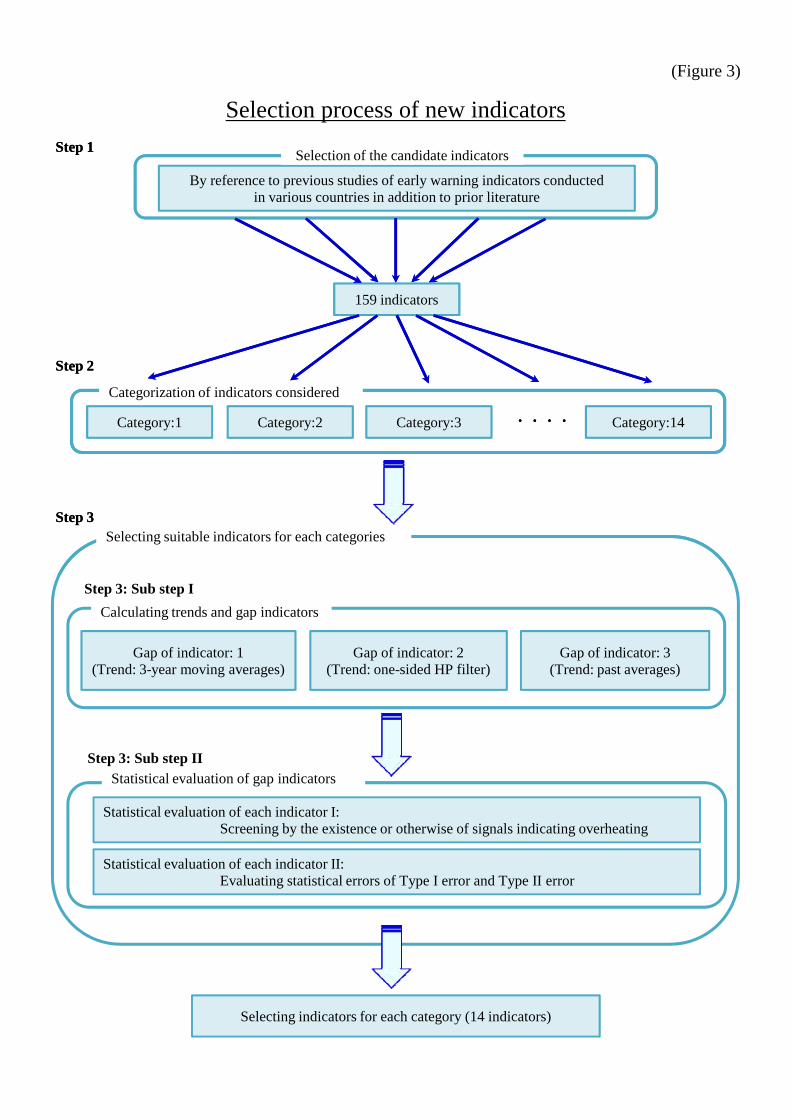
(Figure 3)

Selection process of new indicators

Selecting suitable indicators for each categories

By reference to previous studies of early warning indicators conductedin various countries in addition to prior literature

Selection of the candidate indicators

159 indicators

Categorization of indicators considered

Category:1 Category:2 Category:3 Category:14・・・・

Step 1

Step 2

Step 3

Step 3: Sub step I

Selecting suitable indicators for each categories

Statistical evaluation of gap indicators

Gap of indicator: 1(Trend: 3-year moving averages)

Selecting indicators for each category (14 indicators)

Gap of indicator: 2(Trend: one-sided HP filter)

Gap of indicator: 3(Trend: past averages)

Statistical evaluation of each indicator I: Screening by the existence or otherwise of signals indicating overheating

Statistical evaluation of each indicator II:Evaluating statistical errors of Type I error and Type II error

By reference to previous studies of early warning indicators conductedin various countries in addition to prior literature

Selection of the candidate indicators

159 indicators

Categorization of indicators considered

Category:1 Category:2 Category:3 Category:14・・・・

Step 1

Step 2

Step 3

Step 3: Sub step II

Calculating trends and gap indicators

(Figure 4-1)

Candidate indicators (1)

Sector Sector

1 DI of lending attitudes of financial institutions 43 Volatility of exchange rate

2 DI of lending attitudes of financial institutions (Large firms) 44 Government bond yield volatility

3 DI of lending attitudes of financial institutions (Small firms) 45 Stock purchases on margin to sales on margin ratio

4 ROA from net interest income of banks 46 Stock purchases on margin to TOPIX ratio

5 Current income ROA of banks 47 (Stock purchases on margin + Sales on margin) / TOPIX

6 ROA from operating profits of banks 48 (Stock purchases on margin － Sales on margin) / TOPIX

7 Net income ROA of banks 49 Private investment to GDP ratio

8 Current income ROE of banks 50 Private security investment to GDP ratio

9 ROE from operating profits of banks 51 Private investment (including security investment) to GDP ratio

10 Net income ROE of banks 52 Growth rate of private investment

11 Real loan rate 53 Private fixed investment to GDP ratio

12 Money multiplier (ratio of M2 to the monetary base) 54 Private fixed investment (excluding inventory investment) to GDP ratio

13 Deposits to M2 ratio 55 DSR (Debt service to income ratio)

14 Real deposit outstanding 56 Current balance

15 (Cash + Required reserves) / Total assets 57 Current balance to GDP ratio

16 Financial assets to financial debt ratio 58 Total credit-to-GDP ratio

17 Demand deposit to total liabilities ratio of depository corporations 59 Growth rate of real total credit

18 Loan to deposit ratio of depository corporations 60 Growth rate of total credit

19 Loan to deposit ratio of banks 61 Quarter-on-quarter rate of change in total credit

20 Leverage ratio (Shares and other equities / Assets) 62 Growth rate of total credit － Growth rate of nominal GDP

FinancialInstitutions

PrivateSector

FinancialMarkets

Indicator IndicatorSector Sector

1 DI of lending attitudes of financial institutions 43 Volatility of exchange rate

2 DI of lending attitudes of financial institutions (Large firms) 44 Government bond yield volatility

3 DI of lending attitudes of financial institutions (Small firms) 45 Stock purchases on margin to sales on margin ratio

4 ROA from net interest income of banks 46 Stock purchases on margin to TOPIX ratio

5 Current income ROA of banks 47 (Stock purchases on margin + Sales on margin) / TOPIX

6 ROA from operating profits of banks 48 (Stock purchases on margin － Sales on margin) / TOPIX

7 Net income ROA of banks 49 Private investment to GDP ratio

8 Current income ROE of banks 50 Private security investment to GDP ratio

9 ROE from operating profits of banks 51 Private investment (including security investment) to GDP ratio

10 Net income ROE of banks 52 Growth rate of private investment

11 Real loan rate 53 Private fixed investment to GDP ratio

12 Money multiplier (ratio of M2 to the monetary base) 54 Private fixed investment (excluding inventory investment) to GDP ratio

13 Deposits to M2 ratio 55 DSR (Debt service to income ratio)

14 Real deposit outstanding 56 Current balance

15 (Cash + Required reserves) / Total assets 57 Current balance to GDP ratio

16 Financial assets to financial debt ratio 58 Total credit-to-GDP ratio

17 Demand deposit to total liabilities ratio of depository corporations 59 Growth rate of real total credit

18 Loan to deposit ratio of depository corporations 60 Growth rate of total credit

19 Loan to deposit ratio of banks 61 Quarter-on-quarter rate of change in total credit

20 Leverage ratio (Shares and other equities / Assets) 62 Growth rate of total credit － Growth rate of nominal GDP

21 Depository corporations loans to equity ratio 63 Quarter-on-quarter change in total credit to GDP ratio

22 Financial institutions credit to GDP ratio 64 Household investment to disposable income ratio

23 Growth rate of financial institutions credit 65 Household security investment to disposable income ratio

24 Non-bank credit to GDP ratio 66 Household investment (including security investment) to disposable income ratio

25 Total liabilities to net assets ratio of banks 67 Household security investment to GDP ratio

26 Total assets to total liabilities ratio of banks 68 Household investment to GDP ratio

27 Total assets to net assets ratio of banks 69 Household investment (including security investment) to GDP ratio

28 Ratio of market funding to total liabilities of depository corporations 70 Housing investment to GDP ratio

29 M2 to GDP ratio 71 Housing investment to disposable income ratio

30 Growth rate of M2 72 Household financial risk asset to total financial asset ratio

31 Real M1 73 Household financial assets to GDP ratio

32 Volatility of excess bank stock return 74 Saving rate

33 Equity weighting in institutional investors' portfolios 75 Household loans to GDP ratio

34 Share of overseas investors in stock market 76 Growth rate of household loans

35 Loan rate to deposit rate spread 77 Households' debt-to-cash ratio

36 Growth rate of nominal GDP － Loan rate 78 Household credit to disposable income ratio

37 Growth rate of nominal GDP － Deposit interest rate 79 Growth rate of ratio of household credit to disposable income

38 Long-term / Short-term interest rate spread 80 Household credit to GDP ratio

39 Short-term interest rate 81 Household credit to financial asset ratio

40 Long-term interest rate 82 Household credit to compensation of employee ratio

41 Real long-term interest rate 83 Household credit to cash and deposits ratio

42 Growth rate of real long-term interest rate

FinancialInstitutions

Household

FinancialMarkets

PrivateSector

FinancialMarkets

Indicator Indicator

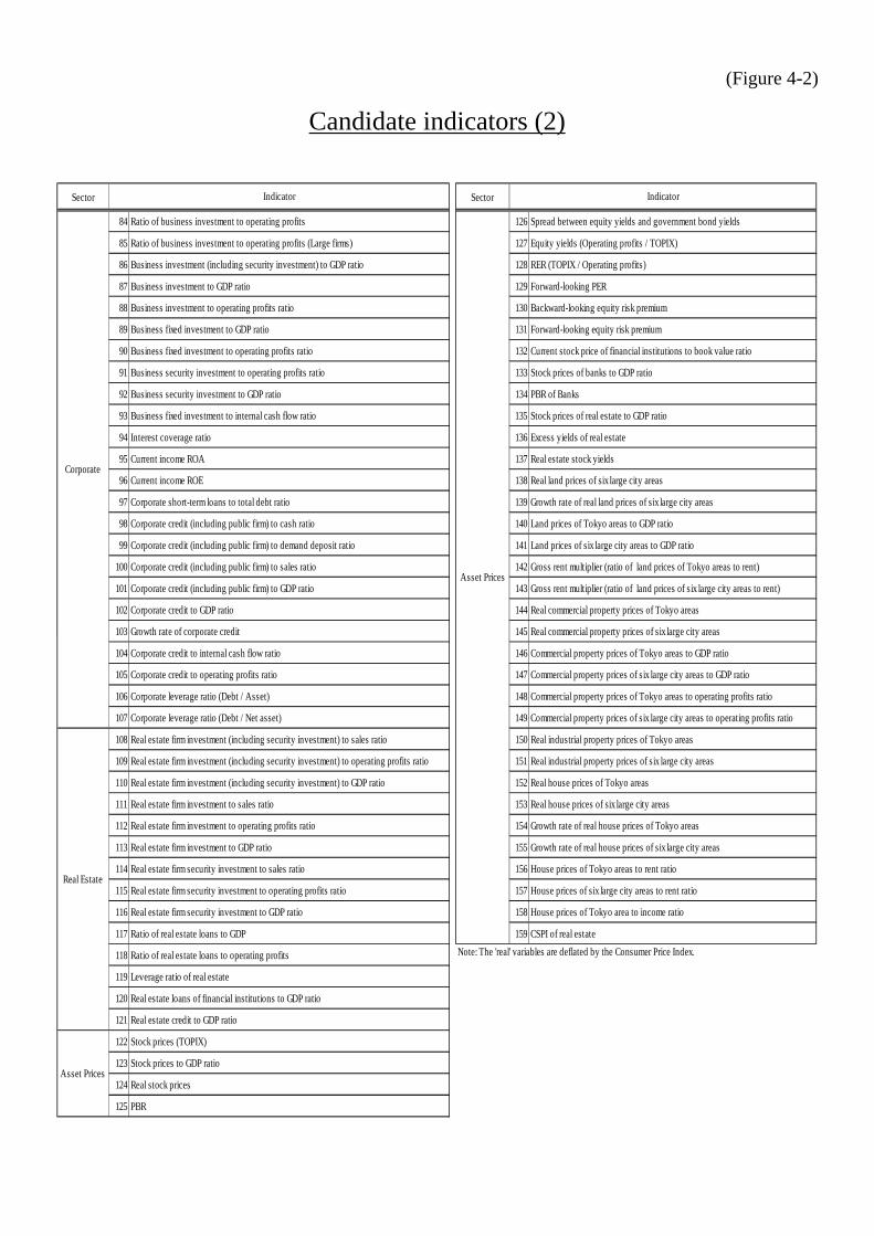
(Figure 4-2)

Candidate indicators (2)

Sector Sector

84 Ratio of business investment to operating profits 126 Spread between equity yields and government bond yields

85 Ratio of business investment to operating profits (Large firms) 127 Equity yields (Operating profits / TOPIX)

86 Business investment (including security investment) to GDP ratio 128 RER (TOPIX / Operating profits)

87 Business investment to GDP ratio 129 Forward-looking PER

88 Business investment to operating profits ratio 130 Backward-looking equity risk premium

89 Business fixed investment to GDP ratio 131 Forward-looking equity risk premium

90 Business fixed investment to operating profits ratio 132 Current stock price of financial institutions to book value ratio

91 Business security investment to operating profits ratio 133 Stock prices of banks to GDP ratio

92 Business security investment to GDP ratio 134 PBR of Banks

93 Business fixed investment to internal cash flow ratio 135 Stock prices of real estate to GDP ratio

94 Interest coverage ratio 136 Excess yields of real estate

95 Current income ROA 137 Real estate stock yields

96 Current income ROE 138 Real land prices of six large city areas

97 Corporate short-term loans to total debt ratio 139 Growth rate of real land prices of six large city areas

98 Corporate credit (including public firm) to cash ratio 140 Land prices of Tokyo areas to GDP ratio

99 Corporate credit (including public firm) to demand deposit ratio 141 Land prices of six large city areas to GDP ratio

100 Corporate credit (including public firm) to sales ratio 142 Gross rent multiplier (ratio of land prices of Tokyo areas to rent)

101 Corporate credit (including public firm) to GDP ratio 143 Gross rent multiplier (ratio of land prices of six large city areas to rent)

102 Corporate credit to GDP ratio 144 Real commercial property prices of Tokyo areas

103 Growth rate of corporate credit 145 Real commercial property prices of six large city areas

Indicator

Corporate

Indicator

Asset Prices

Sector Sector

84 Ratio of business investment to operating profits 126 Spread between equity yields and government bond yields

85 Ratio of business investment to operating profits (Large firms) 127 Equity yields (Operating profits / TOPIX)

86 Business investment (including security investment) to GDP ratio 128 RER (TOPIX / Operating profits)

87 Business investment to GDP ratio 129 Forward-looking PER

88 Business investment to operating profits ratio 130 Backward-looking equity risk premium

89 Business fixed investment to GDP ratio 131 Forward-looking equity risk premium

90 Business fixed investment to operating profits ratio 132 Current stock price of financial institutions to book value ratio

91 Business security investment to operating profits ratio 133 Stock prices of banks to GDP ratio

92 Business security investment to GDP ratio 134 PBR of Banks

93 Business fixed investment to internal cash flow ratio 135 Stock prices of real estate to GDP ratio

94 Interest coverage ratio 136 Excess yields of real estate

95 Current income ROA 137 Real estate stock yields

96 Current income ROE 138 Real land prices of six large city areas

97 Corporate short-term loans to total debt ratio 139 Growth rate of real land prices of six large city areas

98 Corporate credit (including public firm) to cash ratio 140 Land prices of Tokyo areas to GDP ratio

99 Corporate credit (including public firm) to demand deposit ratio 141 Land prices of six large city areas to GDP ratio

100 Corporate credit (including public firm) to sales ratio 142 Gross rent multiplier (ratio of land prices of Tokyo areas to rent)

101 Corporate credit (including public firm) to GDP ratio 143 Gross rent multiplier (ratio of land prices of six large city areas to rent)

102 Corporate credit to GDP ratio 144 Real commercial property prices of Tokyo areas

103 Growth rate of corporate credit 145 Real commercial property prices of six large city areas

104 Corporate credit to internal cash flow ratio 146 Commercial property prices of Tokyo areas to GDP ratio

105 Corporate credit to operating profits ratio 147 Commercial property prices of six large city areas to GDP ratio

106 Corporate leverage ratio (Debt / Asset) 148 Commercial property prices of Tokyo areas to operating profits ratio

107 Corporate leverage ratio (Debt / Net asset) 149 Commercial property prices of six large city areas to operating profits ratio

108 Real estate firm investment (including security investment) to sales ratio 150 Real industrial property prices of Tokyo areas

109 Real estate firm investment (including security investment) to operating profits ratio 151 Real industrial property prices of six large city areas

110 Real estate firm investment (including security investment) to GDP ratio 152 Real house prices of Tokyo areas

111 Real estate firm investment to sales ratio 153 Real house prices of six large city areas

112 Real estate firm investment to operating profits ratio 154 Growth rate of real house prices of Tokyo areas

113 Real estate firm investment to GDP ratio 155 Growth rate of real house prices of six large city areas

114 Real estate firm security investment to sales ratio 156 House prices of Tokyo areas to rent ratio

115 Real estate firm security investment to operating profits ratio 157 House prices of six large city areas to rent ratio

116 Real estate firm security investment to GDP ratio 158 House prices of Tokyo area to income ratio

117 Ratio of real estate loans to GDP 159 CSPI of real estate

118 Ratio of real estate loans to operating profits

119 Leverage ratio of real estate

120 Real estate loans of financial institutions to GDP ratio

121 Real estate credit to GDP ratio

122 Stock prices (TOPIX)

123 Stock prices to GDP ratio

124 Real stock prices

125 PBR

Asset Prices

Indicator

Corporate

Real Estate

Indicator

Note: The 'real' variables are deflated by the Consumer Price Index.

Asset Prices

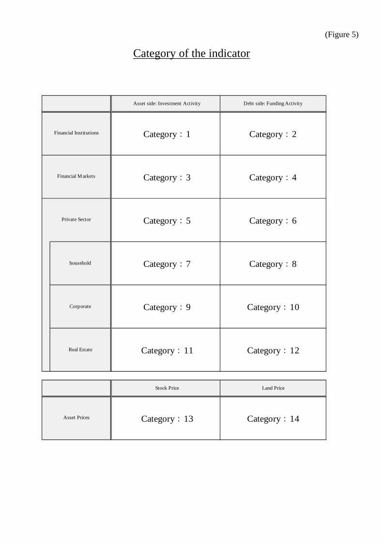
(Figure 5)

Category of the indicator

Asset side: Investment Activity Debt side: Funding Activity

Category：1 Category：2

Category：3 Category：4

Category：5 Category：6

household Category：7 Category：8

Financial Institutions

Financial Markets

Private Sector

Asset side: Investment Activity Debt side: Funding Activity

Category：1 Category：2

Category：3 Category：4

Category：5 Category：6

household Category：7 Category：8

Corporate Category：9 Category：10

Real Estate Category：11 Category：12

Stock Price Land Price

Category：13 Category：14Asset Prices

Financial Institutions

Financial Markets

Private Sector

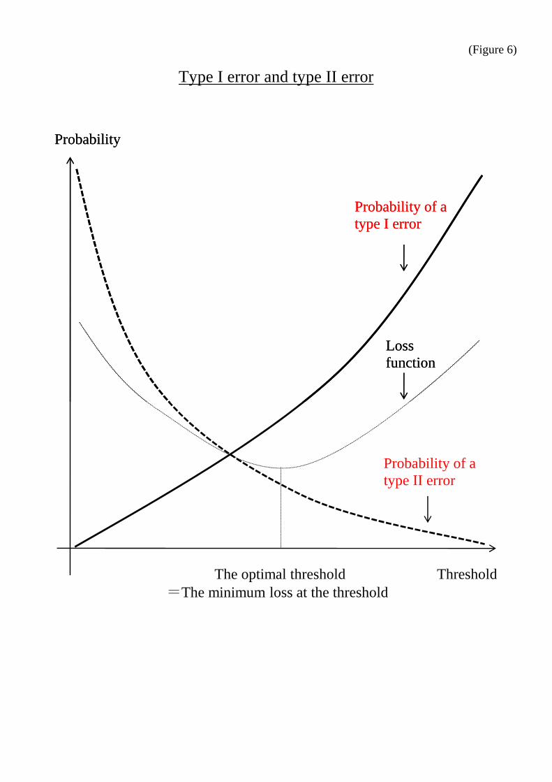
(Figure 6)

Type I error and type II error

Probability of a type I error

Loss function

Probability

ThresholdThe optimal threshold＝The minimum loss at the threshold

Probability of a type I error

Loss function

Probability

Probability of a type II error

(Figure 7)

Selecting indicators of each models

Model Indicator selected Trends Threshold

1.μ = 0.5 DI of lending attitudes of financial institutions past average 1σ

2.μ = 0.7 DI of lending attitudes of financial institutions past average 1σ

3.μ = 0.9 ROA from net interest income of banks one-sided HP filter 1σ

4.NS ratio

1.μ = 0.5 Growth rate of M2 one-sided HP filter 1σ

2.μ = 0.7 Growth rate of M2 one-sided HP filter 1σ

3.μ = 0.9 Non-bank credit to GDP ratio 3-year moving averages 1σ

4.NS ratio Growth rate of M2 one-sided HP filter 1σ

1.μ = 0.5 Equity weighting in institutional investors' portfolios 3-year moving averages 1σ

2.μ = 0.7 Equity weighting in institutional investors' portfolios 3-year moving averages 1σ

3.μ = 0.9 Equity weighting in institutional investors' portfolios 3-year moving averages 1σ

4.NS ratio

1.μ = 0.5 Stock purchases on margin to sales on margin ratio one-sided HP filter 1.25σ

2.μ = 0.7 Stock purchases on margin to sales on margin ratio 3-year moving averages 1σ

3.μ = 0.9 Stock purchases on margin to sales on margin ratio 3-year moving averages 1σ

4.NS ratio

1.μ = 0.5 Private investment to GDP ratio 3-year moving averages 1σ

2.μ = 0.7 Private investment to GDP ratio one-sided HP filter 1.5σ

3.μ = 0.9 Private investment to GDP ratio one-sided HP filter 1σ

4.NS ratio Private investment to GDP ratio 3-year moving averages 1σ

1.μ = 0.5 Total credit-to-GDP ratio one-sided HP filter 1σ

2.μ = 0.7 Total credit-to-GDP ratio 3-year moving averages 1.25σ

3.μ = 0.9 Total credit-to-GDP ratio 3-year moving averages 1σ

4.NS ratio Total credit-to-GDP ratio one-sided HP filter 1σ

1.μ = 0.5 Household investment to disposable income 3-year moving averages 1σ

2.μ = 0.7 Household investment to disposable income one-sided HP filter 1.5σ

3.μ = 0.9 Household investment to disposable income one-sided HP filter 1σ

Financialmarkets

InvestmentActivity

N.A.

FundingActivity

N.A.

Category

Financialinstitutions

InvestmentActivity

N.A.

FundingActivity

Private sector

InvestmentActivity

FundingActivity

InvestmentActivity

Notes: 1. Shaded indicators are one of the indicator of new FAIXs.2. σ is a unit that represents the root mean square of deviation between actual and trend values.

Model Indicator selected Trends Threshold

1.μ = 0.5 DI of lending attitudes of financial institutions past average 1σ

2.μ = 0.7 DI of lending attitudes of financial institutions past average 1σ

3.μ = 0.9 ROA from net interest income of banks one-sided HP filter 1σ

4.NS ratio

1.μ = 0.5 Growth rate of M2 one-sided HP filter 1σ

2.μ = 0.7 Growth rate of M2 one-sided HP filter 1σ

3.μ = 0.9 Non-bank credit to GDP ratio 3-year moving averages 1σ

4.NS ratio Growth rate of M2 one-sided HP filter 1σ

1.μ = 0.5 Equity weighting in institutional investors' portfolios 3-year moving averages 1σ

2.μ = 0.7 Equity weighting in institutional investors' portfolios 3-year moving averages 1σ

3.μ = 0.9 Equity weighting in institutional investors' portfolios 3-year moving averages 1σ

4.NS ratio

1.μ = 0.5 Stock purchases on margin to sales on margin ratio one-sided HP filter 1.25σ

2.μ = 0.7 Stock purchases on margin to sales on margin ratio 3-year moving averages 1σ

3.μ = 0.9 Stock purchases on margin to sales on margin ratio 3-year moving averages 1σ

4.NS ratio

1.μ = 0.5 Private investment to GDP ratio 3-year moving averages 1σ

2.μ = 0.7 Private investment to GDP ratio one-sided HP filter 1.5σ

3.μ = 0.9 Private investment to GDP ratio one-sided HP filter 1σ

4.NS ratio Private investment to GDP ratio 3-year moving averages 1σ

1.μ = 0.5 Total credit-to-GDP ratio one-sided HP filter 1σ

2.μ = 0.7 Total credit-to-GDP ratio 3-year moving averages 1.25σ

3.μ = 0.9 Total credit-to-GDP ratio 3-year moving averages 1σ

4.NS ratio Total credit-to-GDP ratio one-sided HP filter 1σ

1.μ = 0.5 Household investment to disposable income 3-year moving averages 1σ

2.μ = 0.7 Household investment to disposable income one-sided HP filter 1.5σ

3.μ = 0.9 Household investment to disposable income one-sided HP filter 1σ

4.NS ratio Household investment to disposable income 3-year moving averages 1σ

1.μ = 0.5 Household loans to GDP ratio 3-year moving averages 1.25σ

2.μ = 0.7 Household loans to GDP ratio 3-year moving averages 1.25σ

3.μ = 0.9 Household loans to GDP ratio 3-year moving averages 1.25σ

4.NS ratio Household loans to GDP ratio one-sided HP filter 1.5σ

1.μ = 0.5 Business fixed investment to GDP ratio one-sided HP filter 1σ

2.μ = 0.7 Business investment to GDP ratio one-sided HP filter 1σ

3.μ = 0.9 Business investment to GDP ratio one-sided HP filter 1σ

4.NS ratio Business fixed investment to GDP ratio one-sided HP filter 1σ

1.μ = 0.5 Corporate credit to GDP ratio 3-year moving averages 1σ

2.μ = 0.7 Corporate credit to GDP ratio 3-year moving averages 1σ

3.μ = 0.9 Corporate credit to GDP ratio 3-year moving averages 1σ

4.NS ratio Corporate credit to GDP ratio 3-year moving averages 1.25σ

1.μ = 0.5 Real estate firm investment to GDP ratio one-sided HP filter 1σ

2.μ = 0.7 Real estate firm investment to GDP ratio one-sided HP filter 1σ

3.μ = 0.9 Real estate firm investment to GDP ratio one-sided HP filter 1σ

4.NS ratio

1.μ = 0.5 Ratio of real estate loans to GDP one-sided HP filter 1σ

2.μ = 0.7 Ratio of real estate loans to GDP one-sided HP filter 1σ

3.μ = 0.9 Ratio of real estate loans to GDP one-sided HP filter 1σ

4.NS ratio Ratio of real estate loans to GDP one-sided HP filter 1.75σ

1.μ = 0.5 Stock prices one-sided HP filter 1.5σ

2.μ = 0.7 Stock prices one-sided HP filter 1.5σ

3.μ = 0.9 Stock prices one-sided HP filter 1.5σ

4.NS ratio Stock prices one-sided HP filter 1.5σ

1.μ = 0.5 Land prices to GDP ratio 3-year moving averages 1σ

2.μ = 0.7 Land prices to GDP ratio 3-year moving averages 1σ

3.μ = 0.9 Land prices to GDP ratio 3-year moving averages 1σ

4.NS ratio

Financialmarkets

InvestmentActivity

N.A.

FundingActivity

N.A.

Category

Financialinstitutions

InvestmentActivity

N.A.

FundingActivity

Private sector

InvestmentActivity

FundingActivity

Household

InvestmentActivity

FundingActivity

Corporate

InvestmentActivity

FundingActivity

Real estate

InvestmentActivity

FundingActivity

Asset prices

Stock price

Land price

A large number of indicators

N.A.

(Figure 8)

(1) The existing indicators

Comparison between existing FAIXs and new FAIXs

Investment Activity Funding Activity

DI of lending attitudes of financial institutions Money multiplier

< 3-year moving averages, 1σ > < 3-year moving averages, 1σ >

Equity weighting in institutional investors' portfolios

< 3-year moving averages, 1σ >

Total credit-to-GDP ratio

< 3-year moving averages, 1σ >

Households' debt-to-cash ratio

< 3-year moving averages, 1σ >

Ratio of business investment to operating profits Ratio of firms' CP outstanding to their liabilities

< 3-year moving averages, 1σ > < 3-year moving averages, 1σ >

Stock Price Land Price

Stock prices Gross rent multiplier

< 3-year moving averages, 1σ > < 3-year moving averages, 1σ >

Spread between expected equity yields and governmentbond yields

< 3-year moving averages, 1σ >

PrivateSector

Existing Indicators

AssetPrices

FinancialInstitutions

FinancialMarkets

Household

Corporate

(2) Indicators of the new version

Notes: 1. The underlined items show the points of modification. Trends and thresholds for each indicator are inparentheses.

Notes: 2. The symbol represent the following; ‡ : unmodified, *: methods for extracting trends and thresholdsmodified, •: data processing methods modified, †: newly adopted.

Notes: 3. σ is a unit that represents the root mean square of deviation between actual and trend values.

Investment Activity Funding Activity

DI of lending attitudes of financial institutions Money multiplier

< 3-year moving averages, 1σ > < 3-year moving averages, 1σ >

Equity weighting in institutional investors' portfolios

< 3-year moving averages, 1σ >

Total credit-to-GDP ratio

< 3-year moving averages, 1σ >

Households' debt-to-cash ratio

< 3-year moving averages, 1σ >

Ratio of business investment to operating profits Ratio of firms' CP outstanding to their liabilities

< 3-year moving averages, 1σ > < 3-year moving averages, 1σ >

Stock Price Land Price

Stock prices Gross rent multiplier

< 3-year moving averages, 1σ > < 3-year moving averages, 1σ >

Spread between expected equity yields and governmentbond yields

< 3-year moving averages, 1σ >

PrivateSector

Existing Indicators

AssetPrices

FinancialInstitutions

FinancialMarkets

Household

Corporate

Investment Activity Funding Activity

* DI of lending attitudes of financial institutions • Growth rate of M2

< past averages, 1σ > < one-sided HP filter, 1σ >

‡ Equity weighting in institutional investors' portfolios † Stock purchases on margin to sales on margin ratio

< 3-year moving averages, 1σ > < 3-year moving averages, 1σ >

† Private investment to GDP ratio * Total credit-to-GDP ratio

< 3-year moving averages, 1σ > < one-sided HP filter, 1σ >

† Household investment to disposable income ratio • Household loans to GDP ratio

< 3-year moving averages, 1σ > < 3-year moving averages, 1.25σ >

• Business fixed investment to GDP ratio † Corporate credit to GDP ratio

< one-sided HP filter, 1σ > < 3-year moving averages, 1σ >

† Real estate firm investment to GDP ratio † Ratio of real estate loans to GDP

< one-sided HP filter, 1σ > < one-sided HP filter, 1σ >

Stock Price Land Price

* Stock prices • Land prices to GDP ratio

< one-sided HP filter, 1.5σ > < 3-year moving averages, 1σ >

Household

New indicators

FinancialInstitutions

FinancialMarkets

PrivateSector

Corporate

Real Estate

AssetPrices

(Figure 9)

Ratio of firms' CP outstanding to their liabilities

0.8

1.0

1.2

1.4

1.6 Threshold (1 time)

Ratio of firms' CP outstanding to their liabilities

Trends (3-year moving averages)

%

Source: Bank of Japan, "Flow of Funds Accounts."

0.6

0.8

1.0

1.2

1.4

1.6

02 03 04 05 06 07 08 09 10 11 12 13

Threshold (1 time)

Ratio of firms' CP outstanding to their liabilities

Trends (3-year moving averages)

%

CY

Notes: 1. The latest data are as of the October-December quarter of 2013. Notes: 2. The indicator is given by the non-financial corporations' commercial papers outstanding / their

financial liabilities (excluding shares and other equities) × 100.Notes: 3. The sample period begins in Q3 1998, because the CP issuance market was completely liberalized

by abandonment of finance-related notifications and memoranda by Ministry of Finance in June1998.

Notes: 4. The non-financial corporations' commercial papers outstanding and their financial liabilities(excluding shares and other equities) are measured as a four-quarter moving average.

Notes: 5. The financial activity is overheated if the indicator exceeds the shaded area and overcooled if theindicator fall below the shaded area.

(Figure 10)

Spread between expected equity yields and government bond yields

-4

-2

0

2

4

6

8

10

Threshhold (1 time)

Spread between expected equity yields and government bond yields

Trends (3-year moving averages)

%

Sources: Bloomberg; Thomson Reuters.

-6

-4

-2

0

2

4

6

8

10

91 93 95 97 99 01 03 05 07 09 11 13

Threshhold (1 time)

Spread between expected equity yields and government bond yields

Trends (3-year moving averages)

%

CY

Notes: 1. The latest data are as of the January-March quarter of 2014. Notes: 2. The indicator is given by expected equity yields - 10-year JGB yields. Expected equity yield is defined

as an inverse of the one year forward-looking PER of TOPIX.Notes: 3. The financial activity is overheated if the indicator fall below the shaded area and overcooled if the

indicator exceeds the shaded area.

(Figure 11)

Equity weighting in institutional investors' portfolios

10

20

30

40

50

60

70

Threshold (1 time)

Equity weighting in institutional investors' portfolios

Trends (3-year moving averages)

%

Source: Bank of Japan, "Flow of Funds Accounts."

0

10

20

30

40

50

60

70

83 85 87 89 91 93 95 97 99 01 03 05 07 09 11 13

Threshold (1 time)

Equity weighting in institutional investors' portfolios

Trends (3-year moving averages)

%

CY

Notes: 1. The latest data are as of the October-December quarter of 2013. Notes: 2. The indicator is given by the outstanding amount of institutional investors' equity investment / the

outstanding amount of their total security investment × 100. Institutional investors is defined as the insurance sector, the pension funds sector and the securities investment trusts sector.

Notes: 3. The outstanding amount of equity investment and that of total security investment from Q1 1980to Q3 1997 are calculated applying year-on-year rates of changes of the old basis data in those periods.

Notes: 4. The outstanding amount of equity investment and that of total security investment are measuredas a four-quarter moving average.

Notes: 5. The financial activity is overheated if the indicator exceeds the shaded area and overcooled if theindicator fall below the shaded area.

(Figure 12)

(1) The existing Indicator

DI of lending attitudes of financial institutions

-30

-20

-10

0

10

20

30

40

50

80 82 84 86 88 90 92 94 96 98 00 02 04 06 08 10 12 14

Threshold (1 time)

DI of lending attitudes of financial institutions

Trends (3-year moving averages)

% pts

CY

Notes: 1. The latest data are as of the January-March quarter of 2014. Notes: 2. Diffusion index of "Accommodative" minus "Severe".Notes: 3. The financial activity is overheated if the indicator exceeds the shaded area and overcooled if the

indicator fall below the shaded area.

(2) New indicator

Source: Bank of Japan, "Tankan."

-30

-20

-10

0

10

20

30

40

50

80 82 84 86 88 90 92 94 96 98 00 02 04 06 08 10 12 14

Threshold (1 time)

DI of lending attitudes of financial institutions

Trends (3-year moving averages)

% pts

CY

-30

-20

-10

0

10

20

30

40

50

80 82 84 86 88 90 92 94 96 98 00 02 04 06 08 10 12 14

Threshold (1 time)DI of lending attitudes of financial institutionsTrends (past averages)

% pts

CY

Notes: 1. The latest data are as of the January-March quarter of 2014. Notes: 2. Diffusion index of "Accommodative" minus "Severe".Notes: 3. The financial activity is overheated if the indicator exceeds the shaded area and overcooled if the

indicator fall below the shaded area.

Note: 1. For details, see above Notes.

(Figure 13)

(1) The existing indicator

Total credit-to-GDP ratio

100

120

140

160

180

80 82 84 86 88 90 92 94 96 98 00 02 04 06 08 10 12

Threshold (1 time)Total credit-to-GDP ratioTrends (3-year moving averages)

%

CY

Notes: 1. The latest data are as of the October-December quarter of 2013. Notes: 2. The indicator is given by total credit / nominal GDP × 100. Total credit is defined as the sum of the

outstanding amount of loan by private financial institutions to non-financial sector (excluding general government) and the outstanding amount of securities investment by private financial institutions.

Notes: 3. Total credits from Q1 1980 to Q3 1997 are calculated applying year-on-year rates of changes of the old basis data in those periods. Total credits before Q4 1979 are calculated applying year-on-year rates of changes of 1968 SNA basis data in those periods. Nominal GDP from Q1 1980 to Q4 1993 are calculated applying quarter-on-quarter rates of changes of CY2000 basis data in those periods. N i l GDP b f Q4 1979 l l d l i f h f 1968

(2) New indicator

Sources: Cabinet Office, "National accounts"; Bank of Japan, "Flow of Funds Accounts."

100

120

140

160

180

80 82 84 86 88 90 92 94 96 98 00 02 04 06 08 10 12

Threshold (1 time)Total credit-to-GDP ratioTrends (3-year moving averages)

%

CY

100

120

140

160

180

200

80 82 84 86 88 90 92 94 96 98 00 02 04 06 08 10 12

Threshold (1 time)Total credit-to-GDP ratioTrends (one-sided HP filter)

%

CY

Notes: 1. The latest data are as of the October-December quarter of 2013. Notes: 2. The indicator is given by total credit / nominal GDP × 100. Total credit is defined as the sum of the

outstanding amount of loan by private financial institutions to non-financial sector (excluding general government) and the outstanding amount of securities investment by private financial institutions.

Notes: 3. Total credits from Q1 1980 to Q3 1997 are calculated applying year-on-year rates of changes of the old basis data in those periods. Total credits before Q4 1979 are calculated applying year-on-year rates of changes of 1968 SNA basis data in those periods. Nominal GDP from Q1 1980 to Q4 1993 are calculated applying quarter-on-quarter rates of changes of CY2000 basis data in those periods. Nominal GDP before Q4 1979 are calculated applying quarter-on-quarter rates of changes of 1968 SNA basis data in those periods.

Notes: 4. Total credits are measured as a four-quarter moving average.Notes: 5. The financial activity is overheated if the indicator exceeds the shaded area and overcooled if the

indicator fall below the shaded area.

Note: 1. For details, see above Notes.

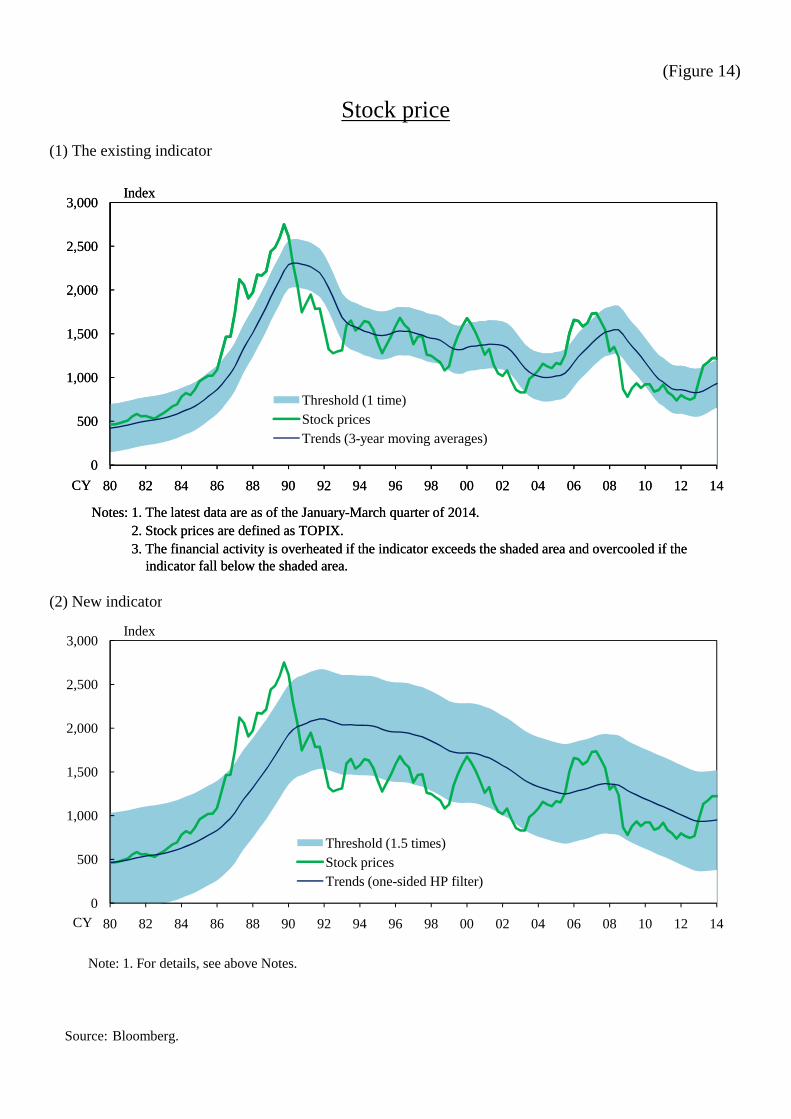
(Figure 14)

(1) The existing indicator

Stock price

0

500

1,000

1,500

2,000

2,500

3,000

80 82 84 86 88 90 92 94 96 98 00 02 04 06 08 10 12 14

Threshold (1 time)Stock pricesTrends (3-year moving averages)

Index

CY

Notes: 1. The latest data are as of the January-March quarter of 2014. Notes: 2. Stock prices are defined as TOPIX.Notes: 3. The financial activity is overheated if the indicator exceeds the shaded area and overcooled if the

indicator fall below the shaded area.

(2) New indicator

Source: Bloomberg.

0

500

1,000

1,500

2,000

2,500

3,000

80 82 84 86 88 90 92 94 96 98 00 02 04 06 08 10 12 14

Threshold (1 time)Stock pricesTrends (3-year moving averages)

Index

CY

0

500

1,000

1,500

2,000

2,500

3,000

80 82 84 86 88 90 92 94 96 98 00 02 04 06 08 10 12 14

Threshold (1.5 times)Stock pricesTrends (one-sided HP filter)

Index

CY

Notes: 1. The latest data are as of the January-March quarter of 2014. Notes: 2. Stock prices are defined as TOPIX.Notes: 3. The financial activity is overheated if the indicator exceeds the shaded area and overcooled if the

indicator fall below the shaded area.

Note: 1. For details, see above Notes.

(Figure 15)

(1) The existing indicator (Money multiplier)

Money

4

5

6

7

8

9

10

11

12

13

14

80 82 84 86 88 90 92 94 96 98 00 02 04 06 08 10 12 14

Threshold (1 time)

Money multiplier (ratio of M2 to the monetary base)

Trends (3-year moving averages)

times

CY

Notes: 1. The latest data are as of the January-February of 2014. Notes: 2. The indicator is given by the average outstanding amount of M2 / the average outstanding amount of

monetary base.Notes: 3. The M2s before Q1 2003 are calculated applying quarter-on-quarter rates of changes of the M2 + CD

in those periods.Notes: 4. The financial activity is overheated if the indicator exceeds the shaded area and overcooled if the

indicator fall below the shaded area

(2) New indicator (Growth rate of M2)

4

5

6

7

8

9

10

11

12

13

14

80 82 84 86 88 90 92 94 96 98 00 02 04 06 08 10 12 14

Threshold (1 time)

Money multiplier (ratio of M2 to the monetary base)

Trends (3-year moving averages)

times

CY

-4

-2

0

2

4

6

8

10

12

14

16

80 82 84 86 88 90 92 94 96 98 00 02 04 06 08 10 12 14

Trends (3-year moving averages)Growth rate of M2Trends (one-sided HP filter)

%

CY

Sources: BOJ, "Monetary base," "Money stock."

Notes: 1. The latest data are as of the January-February of 2014. Notes: 2. The indicator is given by the average outstanding amount of M2 / the average outstanding amount of

monetary base.Notes: 3. The M2s before Q1 2003 are calculated applying quarter-on-quarter rates of changes of the M2 + CD

in those periods.Notes: 4. The financial activity is overheated if the indicator exceeds the shaded area and overcooled if the

indicator fall below the shaded area.

Notes: 1. The latest data are as of the January-February of 2014. Notes: 2. The indicator is given by the growth rate of the average outstanding amount of M2. Notes: 3. The M2s before Q1 2003 are calculated applying quarter-on-quarter rates of changes of the M2 + CD

in those periods.Notes: 4. The financial activity is overheated when the indicator exceeds the shaded area and overcooled when the

indicator below the shaded area.

(Figure 16)

　

(1) The existing indicator (Gross rent multiplier)

Land price

0

50

100

150

200

250

300

80 82 84 86 88 90 92 94 96 98 00 02 04 06 08 10 12

Threshold (1 time)

Gross rent multiplier (ratio of land prices to rent)

Trends (3-year moving averages)

Index, 00/03 = 100

CY

Notes: 1. The latest data are as of the July-September quarter of 2013. Notes: 2. The indicator is given by urban land price index of Tokyo metropolitan area / consumer price index (rent)

for Ku-area of Tokyo × 100.Notes: 3. The land prices before CY 1984 are calculated applying year-on-year rates of changes of the urban land

price index of six large city areas in those periods.Notes: 4. The data of land prices for the intervening half year are linearly interpolated.Notes: 5. The financial activity is overheated if the indicator exceeds the shaded area and overcooled if the

indicator fall below the shaded area.

(2) New indicator (Land prices to GDP ratio)

Sources: Cabinet Office, "National Accounts"; Japan Real Estate Institute, "Urban Land Price Index";Ministry of Internal Affairs and Communications, "Consumer Price Index."

0

50

100

150

200

250

300

80 82 84 86 88 90 92 94 96 98 00 02 04 06 08 10 12

Threshold (1 time)

Gross rent multiplier (ratio of land prices to rent)

Trends (3-year moving averages)

Index, 00/03 = 100

CY

0

50

100

150

200

250

300

350

400

80 82 84 86 88 90 92 94 96 98 00 02 04 06 08 10 12

Threshold (1 time)

Land prices to GDP ratio

Trends (3-year moving averages)

CY

Index, 00/03 = 100

Notes: 1. The latest data are as of the July-September quarter of 2013. Notes: 2. The indicator is given by urban land price index of Tokyo metropolitan area / consumer price index (rent)

for Ku-area of Tokyo × 100.Notes: 3. The land prices before CY 1984 are calculated applying year-on-year rates of changes of the urban land

price index of six large city areas in those periods.Notes: 4. The data of land prices for the intervening half year are linearly interpolated.Notes: 5. The financial activity is overheated if the indicator exceeds the shaded area and overcooled if the

indicator fall below the shaded area.

Notes: 1. The latest data are as of the July-September quarter of 2013. Notes: 2. The indicator is given by urban land price index of six large city areas / nominal GDP × 100.Notes: 3. Nominal GDP from Q1 1980 to Q4 1993 are calculated applying quarter-quarter rates of changes of

CY2000 basis data in those periods. Nominal GDP before Q4 1979 are calculated applying quarter-on-quarter rates of changes of 1968 SNA basis data in those periods.

Notes: 4. The data of land prices for the intervening half year are linearly interpolated.Notes: 5. The financial activity is overheated if the indicator exceeds the shaded area and overcooled if the

indicator fall below the shaded area.

(Figure 17)

(1) The existing Indicator (Ratio of business investment to operating profit)

(2) Ne indicator (B siness fi ed in estment to GDP ratio)

Business fixed investment to GDP ratio

0.0

0.5

1.0

1.5

2.0

2.5

80 82 84 86 88 90 92 94 96 98 00 02 04 06 08 10 12

Trends (1 time)

Ratio of business investment to operating profit

Trends (3-year moving averages)

times

CY

Notes: 1. The latest data are as of the October-December quarter of 2013. Notes: 2. The indicator is given by business investment / operating profits. Business investment is defined as

the sum of fixed investment, inventory investment and security investment.Notes: 3. The financial activity is overheated if the indicator exceeds the shaded area and overcooled if the

indicator fall below the shaded area.

(2) New indicator (Business fixed investment to GDP ratio)

Sources: Cabinet Office, "National accounts"; Ministry of Finance, "Financial Statements Statistics of Corporations byIndustry."

0.0

0.5

1.0

1.5

2.0

2.5

80 82 84 86 88 90 92 94 96 98 00 02 04 06 08 10 12

Trends (1 time)

Ratio of business investment to operating profit

Trends (3-year moving averages)

times

CY

10

12

14

16

18

20

22

80 82 84 86 88 90 92 94 96 98 00 02 04 06 08 10 12

Threshold (1 time)

Business fixed investment to GDP ratio

Trends (one-sided HP filter

%

CY

Notes: 1. The latest data are as of the October-December quarter of 2013. Notes: 2. The indicator is given by business investment / operating profits. Business investment is defined as

the sum of fixed investment, inventory investment and security investment.Notes: 3. The financial activity is overheated if the indicator exceeds the shaded area and overcooled if the

indicator fall below the shaded area.

Notes: 1. The latest data are as of the October-December quarter of 2013. Notes: 2. The indicator is given by business fixed investment / nominal GDP × 100. Notes: 3. Business fixed investment and nominal GDP from Q1 1980 to Q4 1993 are calculated applying quarter-

on-quarter rates of changes of CY2000 basis data in those periods. Business fixed investment and nominalGDP before Q4 1979 are calculated applying quarter-on-quarter rates of changes of 1968 SNA basis datain those periods.

Notes: 4. The financial activity is overheated if the indicator exceeds the shaded area and overcooled if theindicator fall below the shaded area.

(Figure 18)

(1) The existing indicator (Households' debt-to-cash ratio)

Household loans to GDP ratio

0

1

2

3

4

5

83 85 87 89 91 93 95 97 99 01 03 05 07 09 11 13

Trends (1 time)

Households' debt-to-cah ratio

Trends (3-year moving averages)

times

CY

Notes: 1. The latest data are as of the October-December quarter of 2013. Notes: 2. The indicator is given by the households' financial liabilities outstanding / on-hand liquidity.

The on-hand liquidity is defined as the sum of cash and demand deposits. Notes: 3. The financial liabilities, the cash and the demand deposits from Q1 1980 to Q3 1997 are calculated

applying year-on-year rates of changes of the annual data (fiscal year) in those periods. Notes: 4. The financial liabilities, the cash and the demand deposits are measured as a four-quarter moving averages.Notes: 5. The financial activity is overheated if the indicator exceeds the shaded area and overcooled if the

(2) New indicator (Household loans to GDP ratio)

Sources: Cabinet Office, "National accounts"; Bank of Japan, "Flow of Funds Accounts."

0

1

2

3

4

5

83 85 87 89 91 93 95 97 99 01 03 05 07 09 11 13

Trends (1 time)

Households' debt-to-cah ratio

Trends (3-year moving averages)

times

CY

25

30

35

40

45

50

55

60

83 85 87 89 91 93 95 97 99 01 03 05 07 09 11 13

Trends (1.25 times)Household loans to GDP ratioTrends (3-year moving averages)

%

CY

Notes: 1. The latest data are as of the October-December quarter of 2013. Notes: 2. The indicator is given by the households' financial liabilities outstanding / on-hand liquidity.

The on-hand liquidity is defined as the sum of cash and demand deposits. Notes: 3. The financial liabilities, the cash and the demand deposits from Q1 1980 to Q3 1997 are calculated

applying year-on-year rates of changes of the annual data (fiscal year) in those periods. Notes: 4. The financial liabilities, the cash and the demand deposits are measured as a four-quarter moving averages.Notes: 5. The financial activity is overheated if the indicator exceeds the shaded area and overcooled if the

indicator fall below the shaded area.

Notes: 1. The latest data are as of the October-December quarter of 2013. Notes: 2. The indicator is given by the household loans of commercial institutions / nominal GDP × 100. Notes: 3. The household loans of commercial institutions from Q1 1980 to Q3 1997 are calculated applying year-on-

year rates of changes of the annual data (fiscal year) in those periods.Notes: 4. The household loans of commercial institutions are measured as a four-quarter moving average.Notes: 5. For nominal GDP, see figure 13 Note 3.Notes: 6. The financial activity is overheated if the indicator exceeds the shaded area and overcooled if the

indicator fall below the shaded area.

(Figure 19)

Stock purchases on margin to sales on margin ratio

2

4

6

8

10

12

14

16

18

Threshold (1 time)

Stock purchases on margin to sales on margin ratio

Trends (3-year moving averages)

times

Source: Tokyo Stock Exchange, "Outstanding margin trading."

0

2

4

6

8

10

12

14

16

18

84 86 88 90 92 94 96 98 00 02 04 06 08 10 12 14

Threshold (1 time)

Stock purchases on margin to sales on margin ratio

Trends (3-year moving averages)

times

CY

Notes: 1. The latest data are as of the January-March quarter of 2014. Notes: 2. The indicator is given by the stock outstanding purchases on margin / stock outstanding sales on margin. Notes: 3. The financial activity is overheated if the indicator exceeds the shaded area and overcooled if the

indicator fall below the shaded area.

(Figure 20)

Private investment to GDP ratio

20

22

24

26

28

30

32

Threshold (1 time)

Private investment to GDP ratio

Trends (3-year moving averages)

%

Source: Cabinet Office, "National accounts."

18

20

22

24

26

28

30

32

80 82 84 86 88 90 92 94 96 98 00 02 04 06 08 10 12

Threshold (1 time)

Private investment to GDP ratio

Trends (3-year moving averages)

%

CY

Notes: 1. The latest data are as of the October-December quarter of 2013. Notes: 2. The indicator is given by (business fixed investment + inventory investment + housing investment +

durable goods consumption) / nominal GDP × 100.Notes: 3. Business fixed investment, inventory investment, housing investment, and durable goods consumption

from Q1 1980 to Q4 1993 are calculated applying year-on-year rates of changes of CY2000 basis data in those periods. Those figures before Q4 1979 are calculated applying year-on-year rates of changes of 1968 SNA basis data in those periods.

Notes: 4. For nominal GDP, see figure 13 Note 3.Notes: 5. Business fixed investment, inventory investment, housing investment and durable goods consumption are

measured as a four-quarter moving average.Notes: 6. The financial activity is overheated if the indicator exceeds the shaded area and overcooled if the

indicator fall below the shaded area.

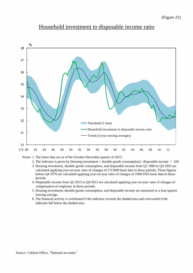
(Figure 21)

Household investment to disposable income ratio

11

12

13

14

15

16

17

18

Threshold (1 time)

Household investment to disposable income ratio

Trends (3-year moving averages)

%

Source: Cabinet Office, "National accounts."

10

11

12

13

14

15

16

17

18

80 82 84 86 88 90 92 94 96 98 00 02 04 06 08 10 12

Threshold (1 time)

Household investment to disposable income ratio

Trends (3-year moving averages)

%

CY

Notes: 1. The latest data are as of the October-December quarter of 2013. Notes: 2. The indicator is given by (housing investment + durable goods consumption) / disposable income × 100. Notes: 3. Housing investment, durable goods consumption, and disposable income from Q1 1980 to Q4 1993 are

calculated applying year-on-year rates of changes of CY2000 basis data in those periods. Those figures before Q4 1979 are calculated applying year-on-year rates of changes of 1968 SNA basis data in those periods.

Notes: 4. Disposable income from Q2 2013 to Q4 2013 are calculated applying year-on-year rates of changes ofcompensation of employee in those periods.

Notes: 5. Housing investment, durable goods consumption, and disposable income are measured as a four-quarter moving average.

Notes: 6. The financial activity is overheated if the indicator exceeds the shaded area and overcooled if theindicator fall below the shaded area.

(Figure 22)

Corporate credit to GDP ratio

130

140

150

160

170

180

190

200

Threshold (1 time)

Corporate credit to GDP ratio

Trends (3-year moving averages)

%

Sources: Cabinet Office, "National accounts"; Bank of Japan, "Flow of Funds Accounts."

120

130

140

150

160

170

180

190

200

83 85 87 89 91 93 95 97 99 01 03 05 07 09 11 13

Threshold (1 time)

Corporate credit to GDP ratio

Trends (3-year moving averages)

%

CY

Notes: 1. The latest data are as of the October-December quarter of 2013. Notes: 2. The indicator is given by the commercial non-financial corporations' financial liabilities (excluding

shares and other equities) / nominal GDP × 100.Notes: 3. The commercial non-financial corporations' financial liabilities from Q1 1980 to Q3 1997 are

calculated applying year-on-year rates of changes of the annual data (fiscal year) in those periods.Notes: 4. For nominal GDP, see figure 13 Note 3.Notes: 5. The commercial non-financial corporations' financial liabilities are measured as a four-quarter

moving averages.Notes: 6. The financial activity is overheated if the indicator exceeds the shaded area and overcooled if the

indicator fall below the shaded area.

(Figure 23)

Real estate firm investment to GDP ratio

-0.2

0.0

0.2

0.4

0.6

0.8

1.0

Threshold (1 time)

Real estate firm capital investment to GDP ratio

Trends (one-sided HP filter)

%

Sources: Cabinet Office, "National accounts"; Ministry of Finance, "Financial Statements Statistics of Corporations byIndustry."

-0.4

-0.2

0.0

0.2

0.4

0.6

0.8

1.0

80 82 84 86 88 90 92 94 96 98 00 02 04 06 08 10 12

Threshold (1 time)

Real estate firm capital investment to GDP ratio

Trends (one-sided HP filter)

%

CY

Notes: 1. The latest data are as of the October-December quarter of 2013. Notes: 2. The indicator is given by (business fixed investment + land investment + inventory investment) / nominal

GDP × 100. Large firms of real estate are counted.Notes: 3. Business fixed investment, land investment, and inventory investment are measured as a four-quarter

moving average. Notes: 4. For nominal GDP, see figure 13 Note 3.Notes: 5. The financial activity is overheated if the indicator exceeds the shaded area and overcooled if the

indicator fall below the shaded area.

(Figure 24)

Ratio of real estate loans to GDP

2

4

6

8

10

12

14

16

18

Threshold (1 time)

Ratio of real estate loans to GDP

Trends (one-sided HP filter)

%

Sources: Cabinet Office, "National accounts"; BOJ, "Loans and bills discounted by sector."

0

2

4

6

8

10

12

14

16

18

80 82 84 86 88 90 92 94 96 98 00 02 04 06 08 10 12

Threshold (1 time)

Ratio of real estate loans to GDP

Trends (one-sided HP filter)

%

CY

Notes: 1. The latest data are as of the October-December quarter of 2013. Notes: 2. The indicator is given by real estate loans of banks / nominal GDP × 100. Notes: 3. Real estate loans of banks are measured as a four-quarter moving average. Notes: 4. For nominal GDP, see figure 13 Note 3.Notes: 5. The financial activity is overheated if the indicator exceeds the shaded area and overcooled if the

indicator fall below the shaded area.

(Figure 25)

Heat Map of existing FAIXs and new FAIXs

(1) Existing FAIXs

(2) New FAIXs

Note: 1. See figure 1 Notes.

80 81 82 83 84 85 86 87 88 89 90 91 92 93 94 95 96 97 98 99 00 01 02 03 04 05 06 07 08 09 10 11 12 13 14

DI of lending attitudes of financial institutions

CY

Financial

80 81 82 83 84 85 86 87 88 89 90 91 92 93 94 95 96 97 98 99 00 01 02 03 04 05 06 07 08 09 10 11 12 13 14CY

DI of lending at titudes of financial inst itut ions

Money multiplier (ratio of M2 to the monetary base)

FinancialMarkets

Equity weighting in inst itutional investors' portfolios

PrivateSector

Total credit-to-GDP rat io

Household Households' debt-to-cash rat io

Ratio of business investment to operat ing profits

Ratio of firms' CP outstanding to their liabilit ies

Spread between expected equity yields and governmentbond yields

Stock prices

Gross rent mult iplier (rat io of land prices to rent)

FinancialInst itut ions

Corporate

Asset Prices

Note: 1. See figure 1 Notes.

Notes: 1. The latest data for DI of lending attitudes of financial institutions, stock purchases on margin to sales onmargin ratio, and stock prices are as of the January-March quarter of 2014. Those for growth rate of M2are as of the January-February of 2014. Those for land prices to GDP ratio are as of the July-Septemberquarter of 2013. Those for other indicators are as of the October-December quarter of 2013.

Notes: 2. See figure 1 Note 2 and 3.

Sources: Bloomberg; Cabinet Office, "National accounts"; Japan Post Holdings, "The former Japan Post statistical data"; Japan Real Estate Institute, "Urban land price index"; Ministry of Finance, "Financial statements statistics of corporations by industry, quarterly"; Ministry of Internal Affairs and Communications, "Consumer price index"; Ministry of Postal Services, "Annual statistical report of postal services," "Annual statistical report of postal service administrations"; Thomson Reuters; Tokyo Stock Exchange,"Outstanding margin trading"; BOJ, "Flow of funds accounts," "Loans and bills discounted by sector,""Monetary base," "Money stock," "Tankan."

80 81 82 83 84 85 86 87 88 89 90 91 92 93 94 95 96 97 98 99 00 01 02 03 04 05 06 07 08 09 10 11 12 13 14

DI of lending attitudes of financial institutions

Growth rate of M2

Equity weighting in institutional investors' portfolios

Stock purchases on margin to sales on margin ratio

Private investment to GDP ratio

Total credit-to-GDP ratio

Household investment to disposable income ratio

Household loans to GDP ratio

Business fixed investment to GDP raito

Corporate credit to GDP ratio

Real estate firm investment to GDP ratio

Ratio of real estate loans to GDP

Stock prices

Land prices to GDP ratio

CY

Real Estate

Asset P rices

Financial

Institutions

Financial

Markets

Private

Sector

Household

Corporate

80 81 82 83 84 85 86 87 88 89 90 91 92 93 94 95 96 97 98 99 00 01 02 03 04 05 06 07 08 09 10 11 12 13 14CY

DI of lending at titudes of financial inst itut ions

Money multiplier (ratio of M2 to the monetary base)

FinancialMarkets

Equity weighting in inst itutional investors' portfolios

PrivateSector

Total credit-to-GDP rat io

Household Households' debt-to-cash rat io

Ratio of business investment to operat ing profits

Ratio of firms' CP outstanding to their liabilit ies

Spread between expected equity yields and governmentbond yields

Stock prices

Gross rent mult iplier (rat io of land prices to rent)

FinancialInst itut ions

Corporate

Asset Prices

(Figure 26)

Receiver operating characteristics curve (1)

(1) Fully informative signal (2) Uninformative signal

0

1

0 1

True positive rate

False positive rate

0

1

0 1

True positive rate

False positive rate

(3) Informative signal

0

1

0 1

True positive rate

False positive rate

0

1

0 1

True positive rate

False positive rate

0

1

0 1

False positive rate

True positive rate

(Figure 27)

Receiver operating characteristics curve (2)

(1) Preference of policy maker (2) Optimal point

0

1

0 1

False positive rate

True positive rate

A

B

0

1

0 1

False positive rate

True positive rate

A

B

(3) ROC curve of total credit to GDP ratio

0

1

0 1

False positive rate

True positive rate

A

B

0

1

0 1

False positive rate

True positive rate

A

B

0

1

0 1

one-sided HP filter

3-year moving averages

True positive rate

False positive rate