Embed Size (px)
Citation preview

This PDF is a selection from an out-of-print volume from the NationalBureau of Economic Research
Volume Title: NBER Macroeconomics Annual 1989, Volume 4
Volume Author/Editor: Olivier Jean Blanchard and Stanley Fischer,editors
Volume Publisher: MIT Press
Volume ISBN: 0-262-02296-6
Volume URL: http://www.nber.org/books/blan89-1
Conference Date: March 10-11, 1989
Publication Date: 1989
Chapter Title: New Indexes of Coincident and Leading Economic Indicators
Chapter Author: James H. Stock, Mark W. Watson
Chapter URL: http://www.nber.org/chapters/c10968
Chapter pages in book: (p. 351 - 409)
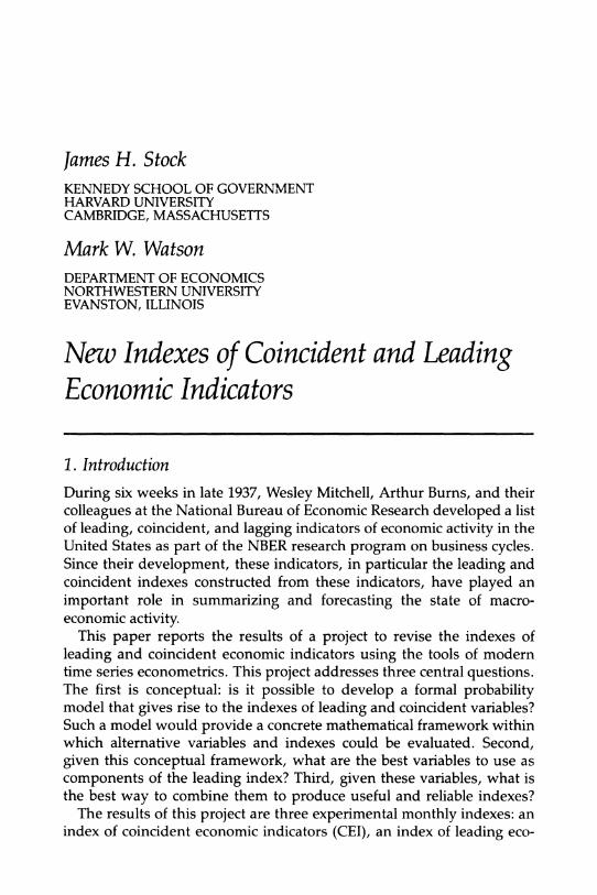
James H. Stock KENNEDY SCHOOL OF GOVERNMENT HARVARD UNIVERSITY CAMBRIDGE, MASSACHUSETTS
Mark W. Watson DEPARTMENT OF ECONOMICS NORTHWESTERN UNIVERSITY EVANSTON, ILLINOIS
New Indexes of Coincident and Leading Economic Indicators
1. Introduction
During six weeks in late 1937, Wesley Mitchell, Arthur Burns, and their
colleagues at the National Bureau of Economic Research developed a list of leading, coincident, and lagging indicators of economic activity in the United States as part of the NBER research program on business cycles. Since their development, these indicators, in particular the leading and coincident indexes constructed from these indicators, have played an
important role in summarizing and forecasting the state of macro- economic activity.
This paper reports the results of a project to revise the indexes of
leading and coincident economic indicators using the tools of modern time series econometrics. This project addresses three central questions. The first is conceptual: is it possible to develop a formal probability model that gives rise to the indexes of leading and coincident variables? Such a model would provide a concrete mathematical framework within which alternative variables and indexes could be evaluated. Second, given this conceptual framework, what are the best variables to use as components of the leading index? Third, given these variables, what is the best way to combine them to produce useful and reliable indexes?
The results of this project are three experimental monthly indexes: an index of coincident economic indicators (CEI), an index of leading eco-
352 * STOCK & WATSON
nomic indicators (LEI), and a Recession Index. The experimental CEI
closely tracks the coincident index currently produced by the Depart- ment of Commerce (DOC), although the methodology used to produce the two series differs substantially. The growth of the experimental CEI is also highly correlated with the growth of real GNP at business cycle frequencies. The proposed LEI is a forecast of the growth of the pro- posed CEI over the next six months constructed using a set of leading variables or indicators. The Recession Index, a new series, is the probabil- ity that the economy will be in a recession six months hence, given data available through the month of its construction.
This article is organized as follows. Section 2 contains a discussion of the indexes and a framework for their interpretation. Section 3 presents the experimental indexes, discusses their construction, and examines their within-sample performance. In Section 4, the indexes are consid- ered from the perspective of macroeconomic theory, focusing in particu- lar on several salient series that are not included in the proposed leading index. Section 5 concludes.
2. Making Sense of the Coincident and Leading Indexes 2.1 THE COINCIDENT INDEX
The coincident and leading economic indexes have been widely fol- lowed in business and government for decades, yet have received sur-
prisingly little attention from academic economists.1 We suggest that one
important reason for this neglect is that it is unclear what the existing CEI and LEI measure. That is, with what are the coincident indicators coincident? What do the leading indicators lead? Burns and Mitchell's (1938, 1946) answer was that the coincident indicators are coincident with the "reference cycle," that is, with the broad-based swings in eco- nomic activity known as the business cycle. This definition has intuitive
appeal but, as Burns and Mitchell (1946, p. 76) recognized, lacks precise mathematical content. It is therefore unclear what conclusions one should draw from swings in the index.
To clarify the issues concerning the reference cycle, it is useful to consider how one might construct a monthly coincident index were real GNP data available accurately on a monthly basis. Would it be appropri- ate simply to let swings in GNP define the reference cycle? The "business
1. Exceptions include Auerbach (1982), Diebold and Rudebusch (1987), Hymans (1973), Kling (1987), Koch and Raasche (1988), the papers in Moore (1983), Neftci (1982), Stekler and Schepsman (1973), Vaccara and Zarnowitz (1978), Wecker (1979), Zarnowitz and Moore (1982), and Zellner, Hong, and Gulati (1987). One of Koopmans' (1947) criticisms of Burns and Mitchell (1946) is their lack of a formal statistical framework in which to interpret their results.
New Indexes of Coincident and Leading Economic Indicators * 353
cycle" commonly refers to co-movements in different forms of economic activity, not just fluctuations in GNP; see Lucas (1977) for a discussion of this point. This suggests taking as primitive Bums and Mitchell's (1946, p. 3) definition that a business cycle "consists of expansions occurring at about the same time in many economic activities, followed by similarly general recessions, contractions, and revivals. .. ." If so, it would be incorrect to define a recession solely in terms of monthly GNP. For
example, suppose that a drought dramatically reduces agricultural out-
put but that output in other sectors remains stable, so that aggregate unemployment remains steady. This scenario does not fit Burns and Mitchell's definition of a recession even if the decline in GNP is sus- tained. Rather, the reference cycle reflects co-movements in a broad
range of macroeconomic aggregates such as output, employment, and sales.
The model adopted in this research formalizes the idea that the refer- ence cycle is best measured by looking at co-movements across several
aggregate time series. The experimental CEI is an estimate of the value of a single unobserved variable, "the state of the economy," denoted by Ct. This unobserved variable is defined by assuming that the co- movements of observed coincident time series at all leads and lags arise
solely from movements in Ct. Of course, any particular coincident series, such as industrial production, might move in ways that are not associ- ated with this unobserved variable. Thus each roughly coincident series is thought of as having a component attributable to the single unob- served variable, plus a unique (or "idiosyncratic") component. Each idio- syncratic component is assumed to be uncorrelated with the other idio- syncratic components and with the unobserved common "state of the economy" at all leads and lags.
Technically, this amounts to specifying an "unobserved single index" or "dynamic factor" model for the coincident variables of the type consid- ered by, for example, Geweke (1977), Sargent and Sims (1977), and Engle and Watson (1981). The major features of the model and estimation procedure are summarized here, and the details are given in Stock and Watson (1988a). Let Xt denote an n x 1 vector of the logarithms of macroeconomic variables that are hypothesized to move contemporane- ously with overall economic conditions. In the single-index model, Xt consists of two stochastic components: the common unobserved scalar variable, or "index," Ct, and an n-dimensional component, ut, that repre- sents idiosyncratic movements in the series and measurement error. Both the unobserved index and the idiosyncratic component are mod- eled as having linear stochastic structures. Looking ahead to the empiri- cal results, the coincident variables used in the analysis appear to be
354 * STOCK & WATSON
integrated but not cointegrated, so that model is specified in terms of AXt and ACt.2 This suggests the formulation:
AX, = p + y(L)AC, + u, (1)
D(L)u = et (2)
O(L)ACt = 5 + tt, (3)
where L denotes the lag operator, and +(L), y(L) and D(L) are respec- tively scalar, vector, and matrix lag polynomials.
The main identifying assumption expresses the core notion of the
dynamic factor model that the co-movements of the multiple time series arise from the single source ACt. This is made precise by assuming that
(ut, , u. . , , ACt) are mutually uncorrelated at all leads and lags, which is achieved by making D(L) diagonal and the n + 1 disturbances (Et, . . .,Ent, rt) mutually and serially uncorrelated. In addition, ACt is assumed to enter at least one of the variables in (1) only contemporane- ously. The system is estimated by maximum likelihood using the Kalman filter. The proposed CEI is computed as the minimum mean
square error linear estimate of this single common factor, C,tt, produced by applying the Kalman filter to the estimated system. Thus C,tt is a linear combination of current and past logarithms of the coincident variables.
It is tempting to interpret the single index specification as implying that there is a single causal source of common variation (or shock) among the real variables Xt (theoretical models can be developed in which this is the case; see Altug (1984) or Sargent and Sims (1977) for discussions). But one
ought not read too much into the factor formulation. With three serially uncorrelated variables (the time series analog of a factor model of cross- sectional variables), the model lacks empirical content: Its parameters are
exactly identified, so the various shocks that comprise the errors can
always be recast in a single index form, and the factor merely summarizes the covariance among the three series. When there are more than three observable series or when the variables are serially correlated, the dy- namic factor model is overidentified. Imposing y(L) = yo (as is done below for all but one of the coincident variables) further restricts the impulse
2. As an empirical matter, many macroeconomic time series are well characterized as containing stochastic trends; see, for example, Nelson and Plosser (1982). Were these stochastic trends to enter only through C, then Xt would contain a single common stochastic trend. Thus X, would be cointegrated of order n-1 as defined by Engle and Granger (1987). For the coincident series considered here, however, this appears not to be the case: the hypothesis that the coincident series individually contain a stochastic trend cannot be rejected, but neither can the hypothesis that there is no cointegration among these variables.
New Indexes of Coincident and Leading Economic Indicators * 355
response from Tt to AXt to be proportional across the observable series. One interpretation of these restrictions is that there are multiple sources of economic fluctuations, but that they have proportional dynamic effects on the real variables. That is, the combination of shocks that induce busi- ness cycles might vary from one cycle to the next, but to a statistically good approximation, the relative movements of the components of AXt in
response to these shocks is the same.3
2.2 THE LEADING INDEX
Given this definition of the CEI, the next question is how to construct a
leading index. The proposed LEI is the estimate of the growth of this unobserved factor over the next six months, computed using a set of
leading variables; in the notation of (1)-(3), this is Ct+6[t-Ctlt. This repre- sents a conceptual break with the existing DOC leading index. The objec- tive of the historical NBER approach was to produce a series in levels, with
turning points that preceded the reference cycle by several months. Thus the original NBER and the current DOC leading indexes can be thought of as forecasts of the level of the CEI several months hence. To the extent that one is interested in the relative growth rather than the absolute level of economic activity, however, it is more useful to forecast the growth of Ct. Forecasts of growth and future levels are, of course, closely linked: be- cause the LEI is Ct+61t-CtCt, and the CEI is Ctlt, the sum of the CI and the LEI is Ct+61,t which is a forecast of the (log) level of the CEI six months hence.
The LEI is constructed by modeling the leading variables (Yt) and the unobserved state of the economy (Ct) as a vector autoregressive system with two modifications. First, the formulation recognizes Ct is unob- served. Second, the number of parameters to be estimated has been reduced by eliminating higher lags of the variables in all equations of the
system except the equation for the coincident variable. The specific model estimated is the reduced form simultaneous equation system,
ACt = ,-c + Acc(L)ACt-1 + Acy(L)Yt_1 + vct (4)
Yt = Ly + Ayc(L)ACt-1 +AYY(L)Yt-1 + VYt, (5)
where (vct, vyt) are serially uncorrelated error terms. The orders of the lag polynomials Acc(L), Acy(L), Ayc(L), and Ay(L) were determined empirically using statistical criteria; the details are discussed in the next section. The leading variables Yt were transformed as necessary to appear stationary.
3. More than one factor is typically used to fit models containing both real and nominal variables. For example, Singleton (1980) finds that two factors are necessary in a system containing yields on three-month, six-month, one-year, and five-year government secu- rities, the unemployment rate, and manufacturers' shipments.
356 * STOCK & WATSON
The parameters of the coincident and leading models are estimated in two steps. In the first step, the parameters of the coincident model (1)- (3) are estimated by maximum likelihood, where the Kalman filter is used to evaluate the likelihood function. In the second step, the leading model is estimated conditional on the estimated parameters of the coinci- dent model. Technically, (1), (2), (4), and (5) are combined to form a state space model, with ACt and its lags being unobserved elements of the state vector. The parameters of (4) and (5) are then estimated by maxi- mum likelihood (using the EM algorithm), conditional on the estimates of the parameters of (1) and (2). A desirable consequence of this two-step procedure is that the coincident index (Ctlt), constructed as a weighted average of AXt using (1)-(3), is consistent with the implicit definition of Ct in the full model (1), (2), (4), and (5). The main benefit of this approach is that it prevents potential misspecification in (4) and (5) from inducing inconsistency in the parameters of (1) and (2). The cost of this benefit is
potential inefficiency: if the full system is correctly specified, the two-
step procedure will produce consistent but inefficient estimators relative to the M.L.E. for the complete system (1), (2), (4), and (5). Thus the simplest way to think of the leading model is as a projection of AC,tl onto leading variables in vector autoregressive (VAR) framework, except that the lack of observability of ACtit is handled explicitly. Finally, the LEI is computed as Ct+6t1-C1tl from the estimated model (1), (2), (4), and (5). Movements in the LEI arising from Xt are negligibly small and will be ignored to simplify the discussion below.
2.3 PREDICTIONS OF RECESSIONS AND EXPANSIONS
A traditional role of the LEI has been to signal future recessions and recoveries; indeed, it was to provide such signals that Mitchell and Burns (1938) developed their original list of indicators.4 The value of identifying and forecasting cyclical turning points has been a matter of controversy among academic economists. One interpretation of this controversy is that the concepts of expansion and recession are incorrectly perceived to embody a view of the dynamic evolution of the economy that is at odds with the probabilistic foundations of formal macroeconomic models.
In forecasting turning points, recessions and expansions are treated as conceptually distinct objects, perhaps associated with fundamentally dif- ferent behavior of the economy. In contrast, the structure of standard macroeconomic models does not change from an expansion to a contrac- tion: in terms of the underlying theory of behavior, a month that falls in a
4. Moore (1979) recounts how the list was developed at the request of Treasury Secretary Morgenthau and evaluates the out-of-sample performance of the original series.
New Indexes of Coincident and Leading Economic Indicators ? 357
recession does not differ fundamentally from a month that falls in an
expansion. To simplify the argument only slightly, traditional business
cycle analysis is associated with treating recessions and expansions as
periods of distinctly different economic behavior, defined by intrinsic shifts (essential nonlinearities) in the macroeconomic process by which the data are generated. The alternative view is that expansions and recessions have no intrinsic content, in the sense that they are not associ- ated with fundamental shifts in the behavior of the economy, but rather are the results of a stable structure adapting to random shocks. Accord-
ing to this latter view, recessions and expansions are extrinsic patterns, not intrinsic macroeconomic shifts.5
The model described in the previous subsection is consistent with the "extrinsic" view: recessions and expansions are generated by certain
configurations of random shocks to a linear time series model. Yet this does not invalidate the concept or the importance of forecasting business
cycles. Recessions are important political, social, and economic events. Periods of prolonged, widespread expansion provide opportunities to workers and bounty to consumers; the most severe periods of contrac- tion threaten governments and even forms of government. Thus the
question becomes: is it possible to forecast those politically and socially important events that will come to be termed expansions and contrac- tions? Can these patterns be recognized in advance?
The Recession Index is an estimate of the probability that the economy will be in a recession six months hence. This probability is computed using the same time series model used to calculate the proposed LEI, and is based on a definition (in terms of the sample path of ACt) of what constitutes a recession and an expansion. Unfortunately, it is difficult to
quantify precisely those patterns that will be recognized as expansions or contractions. Burns and Mitchell (1946, p. 3) considered the minimum
period for a full business (reference) cycle to be one year; in practice, the shortest expansions and contractions they identified were six months. The Recession Index is computed by approximating a recessionary (ex- pansionary) period in terms of negative (positive) growth of the CEI that lasts at least six months.6
5. Slutzky (1937) and Adelman and Adelman (1959) can be interpreted as arguing for the "extrinsic" view; Neftci (1982) and Hamilton (1987) develop techniques consistent with the "intrinsic" view. This debate is related to the distinction between exogenous shocks and endogenous instability being the source of aggregate fluctuations. The extrinsic/ intrinsic terminology focuses on the identification and interpretation of recessions and expansions.
6. More precisely, a recession and an expansion are determined by partitioning future AC, into three regions, or patterns. We define a month to be in a recessionary pattern if that month is either in a sequence of six consecutive declines of C, below some boundary b,,, or
358 * STOCK & WATSON
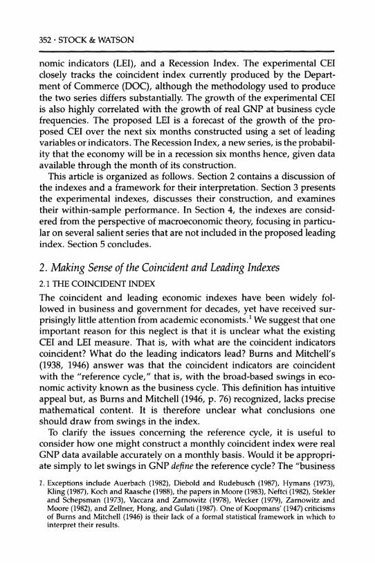
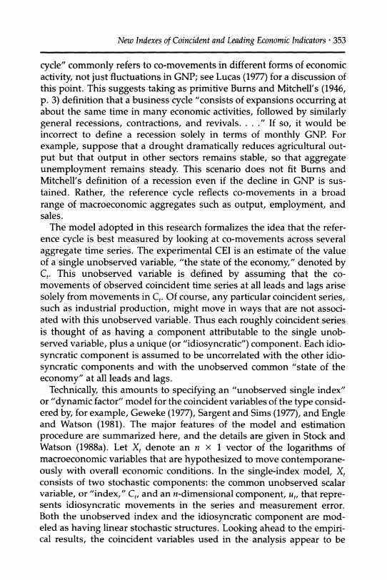
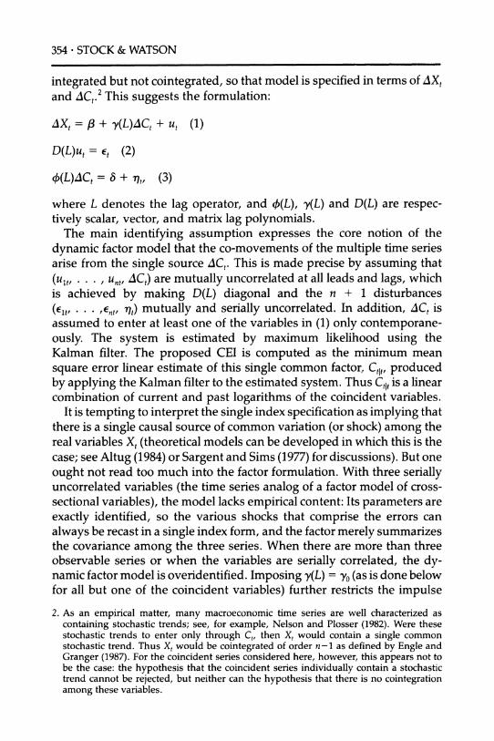
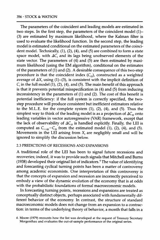
3. The Revised Indexes The proposed CEI is plotted in Figure 1, the proposed LEI is plotted in Figure 2, and the proposed Recession Index is plotted in Figure 3. The vertical lines in these and subsequent figures represent the official ex post NBER-dated cyclical turning points.
3.1 THE INDEX OF COINCIDENT ECONOMIC INDICATORS
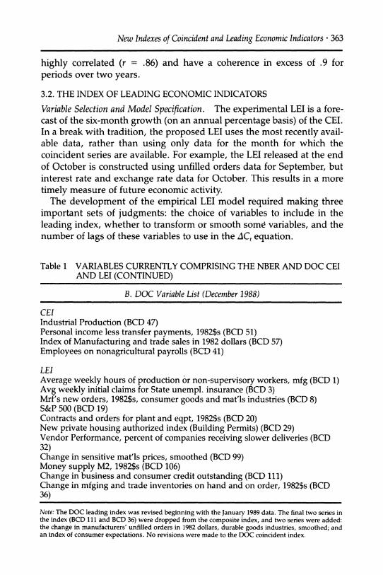
Data and Empirical Results. The variables entering the proposed CEI and LEI, as well as the variables entering the current DOC coincident and leading indexes, are listed in Table 1. The proposed CEI is based on four series: industrial production, real personal income less transfer pay- ments, real manufacturing and trade sales, and employee-hours in
nonagricultural establishments. These are the series currently used by the DOC to construct its coincident index, except that the total number of employees (rather than employee-hours) is used in the Commerce series.7 The data were obtained from the January 31, 1989 release of CITIBASE. Empirical results are computed using data starting in 1959:1.
The empirical results for the single-index model, specified with em-
ployment rather than employee-hours, are discussed in detail in Stock and Watson (1988b); the results for the model estimated with employee- hours are summarized here. Preliminary data analysis suggested model- ing the logarithms of these four series as being individually integrated but not cointegrated. Dickey-Fuller (1979) tests were unable to reject the null hypothesis that each of the series are individually integrated. The Stock-Watson (1988a) qf test of the null hypothesis that the four series are not cointegrated against the alternative that there is at least one coin- tegrating vector (computed using four lags of the series and a linear time trend) yielded a statistic of -25.25, with a p-value of 60%. Similar evi-
is in a sequence of nine declines below the boundary with no more than one increase during the middle seven months. Thus a recessionary pattern is the union of 15 sets contained in g17. An expansionary pattern is defined analogously, with "increases" replac- ing "declines" and b, replacing brt. This does not exhaust all possible patterns, and the remaining patterns are said to be indeterminate. Reasonable people might disagree on these boundaries: these regions might constitute fuzzy sets. This "fuzziness" is quantified by making b, and bet normally distributed random variables. After ruling out the possibil- ity that a given month falls in neither region, the NBER Recession Index is computed as the probability (given currently available data) that, six months hence, the time path of Ct will fall in a recession region. This entails integrating a 17-dimensional normal density conditional on (b,, bet), which in turn have independent normal distributions.
7. We follow Moore's (1988) recommendation and use employee-hours rather than the number of employees in constructing the CEI. Because of overtime and part-time work, employee-hours measures more directly fluctuations in labor input than does the num- ber of employees.

New Indexes of Coincident and Leading Economic Indicators ? 359
dence of non-cointegration was obtained from pairwise residual-based tests for cointegration as proposed by Engle and Granger (1987). The subsequent analysis therefore uses first differences of the logarithms of these series (AXt).
Geweke (1977) and Sargent and Sims (1977) point out that the single index model (1)-(3) imposes testable restrictions on the spectral density matrix of the vector time series. Because ACt and ut are by assumption uncorrelated at all leads and lags, (1) implies that Sax(c) =
y(e-i?s)Sc((o)y(ei)), + S(co), where Sx(co) denotes the spectral density matrix of AXt at frequency w, etc. Because Sac(w) is a scalar and Su(w) is diagonal, this provides testable restrictions on SaX(w). Performing this test for the coincident indicator model over six equally-spaced bands constructed using AXt (the unconstrained estimate of the spectrum is the averaged matrix periodogram) provides little evidence against the restrictions imposed by the dynamic single-index structure: the x30 test statistic is 19.8, having a p-value of 92%.
Figure 1 THE PROPOSED INDEX OF COINCIDENT ECONOMIC INDICATORS
0
9- / Ie 0
t\ -
O
O--
0-
'-I / 0 -
?- ^ i
0 CD
60 62 64 66 68 70 72 74 76 78 80 82 84 86 88
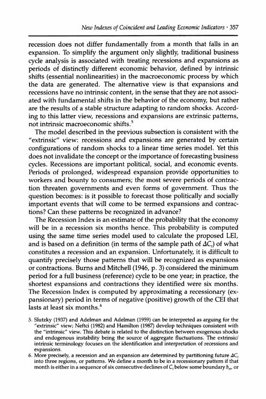
360 - STOCK & WATSON
Figure 2 THE PROPOSED INDEX OF LEADING ECONOMIC INDICATORS
t-
a. LO
c
*
I_ I I I I I I I I I I I I I I I I I .1 A I 1 1 I
1 60 62 64 66 68 70 72 74 76 78 80 82 84 86 88
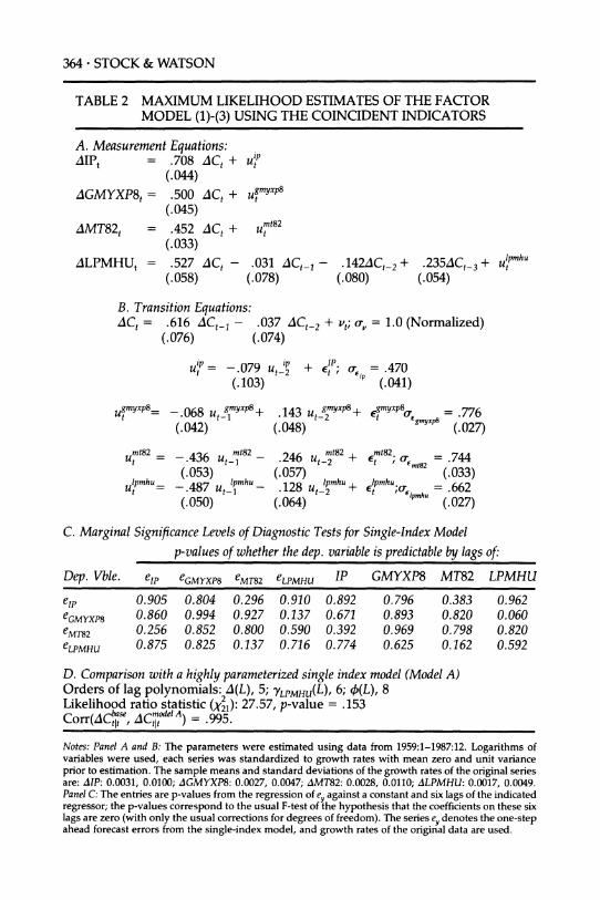
The maximum likelihood estimates of the parameters of the single index model (1)-(3) are presented in Table 2. A specification in which the factor enters each of the four equations only contemporaneously (i.e., y(L) = y0) was found to be inconsistent with the data.8 This is not the case, however, when lags of AC, are permitted to enter the employee- hours equation: as indicated in panel B of Table 2, various diagnostic statistics provide no statistical evidence of (linear) misspecification of this model. Thus employment is better modeled as a slightly lagging rather than an exactly coincident variable.
As a further check on the fit of the model, several highly parameter- ized versions were estimated; the results for one specification are summa- rized in Table 2(D). The additional parameters are not statistically signifi- cant at the 5% level, and the Ctlt series created using these specifications are essentially indistinguishable from the CEI reported above. are essentially indistinguishable from the CEI reported above.
8. With y(L) = y0, the one-step ahead forecast errors for employee-hours were correlated with past observations on AXt.

New Indexes of Coincident and Leading Economic Indicators * 361
Figure 3 THE PROPOSED RECESSION INDEX
0
Co
02 I I N
o I..1.L.. ,..J . l.. .l 0 60 62 64 66 68 70 72 74 76 78 80 82 84 86 88
The proposed CEI, the DOC coincident index, and real GNP growth. The
proposed CEI is graphed in Figure 1. The figure portrays Ctlt computed using the empirical model in Table 2, then exponentiated and scaled to
equal 100 in July 1967. Visual inspection indicates that the cyclical peaks and troughs of the CEI coincide with the official NBER-dated turning points, with the exception of 1969, when the peak in the proposed series occurs two months prior to the official NBER turning point.
The proposed CEI is quantitatively similar to the existing DOC coinci- dent index; both are graphed in Figure 4(a). The main differences are the
slightly greater trend growth and cyclical volatility of the DOC series. The correlation between the growth rates of the proposed and DOC series is .95, and the average coherence for periods exceeding eight months is .97.9
9. This high coherence at low frequencies suggests that the population joint spectral den- sity matrix of the proposed CEI and the DOC index might be singular at frequency zero, i.e., the two series might be cointegrated; but the series are constructed using different implicit weights on AX,, and there is no statistical evidence against non-cointegration.
362 - STOCK & WATSON
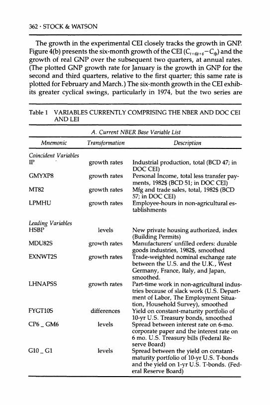
The growth in the experimental CEI closely tracks the growth in GNP.
Figure 4(b) presents the six-month growth of the CEI (Ct+61t+6- Ctl) and the
growth of real GNP over the subsequent two quarters, at annual rates. (The plotted GNP growth rate for January is the growth in GNP for the second and third quarters, relative to the first quarter; this same rate is
plotted for February and March.) The six-month growth in the CEI exhib- its greater cyclical swings, particularly in 1974, but the two series are
Table 1 VARIABLES CURRENTLY COMPRISING THE NBER AND DOC CEI AND LEI
A. Current NBER Base Variable List
Mnemonic Transformation Description Coincident Variables
Coincident Variables IP
GMYXP8
MT82
LPMHU
Leading Variables HSBP
MDU82S
EXNWT2S
LHNAPSS
FYGT1OS
CP6_ GM6
G10 G1
growth rates
growth rates
growth rates
growth rates
Industrial production, total (BCD 47; in DOC CEI) Personal Income, total less transfer pay- ments, 1982$ (BCD 51; in DOC CEI) Mfg and trade sales, total, 1982$ (BCD 57; in DOC CEI) Employee-hours in non-agricultural es- tablishments
levels New private housing authorized, index (Building Permits)
growth rates Manufacturers' unfilled orders: durable goods industries, 1982$, smoothed
growth rates Trade-weighted nominal exchange rate between the U.S. and the U.K., West Germany, France, Italy, and Japan, smoothed.
growth rates Part-time work in non-agricultural indus- tries because of slack work (U.S. Depart- ment of Labor, The Employment Situa- tion, Household Survey), smoothed
differences Yield on constant-maturity portfolio of 10-yr U.S. Treasury bonds, smoothed
levels Spread between interest rate on 6-mo. corporate paper and the interest rate on 6 mo. U.S. Treasury bills (Federal Re- serve Board)
levels Spread between the yield on constant- maturity portfolio of 10-yr U.S. T-bonds and the yield on 1-yr U.S. T-bonds. (Fed- eral Reserve Board)
New Indexes of Coincident and Leading Economic Indicators * 363
highly correlated (r = .86) and have a coherence in excess of .9 for
periods over two years.
3.2. THE INDEX OF LEADING ECONOMIC INDICATORS
Variable Selection and Model Specification. The experimental LEI is a fore- cast of the six-month growth (on an annual percentage basis) of the CEI. In a break with tradition, the proposed LEI uses the most recently avail- able data, rather than using only data for the month for which the coincident series are available. For example, the LEI released at the end of October is constructed using unfilled orders data for September, but interest rate and exchange rate data for October. This results in a more
timely measure of future economic activity. The development of the empirical LEI model required making three
important sets of judgments: the choice of variables to include in the
leading index, whether to transform or smooth some variables, and the number of lags of these variables to use in the ACt equation.
Table 1 VARIABLES CURRENTLY COMPRISING THE NBER AND DOC CEI AND LEI (CONTINUED)
B. DOC Variable List (December 1988)
CEI Industrial Production (BCD 47) Personal income less transfer payments, 1982$s (BCD 51) Index of Manufacturing and trade sales in 1982 dollars (BCD 57) Employees on nonagricultural payrolls (BCD 41)
LEI Average weekly hours of production or non-supervisory workers, mfg (BCD 1) Avg weekly initial claims for State unempl. insurance (BCD 3) Mrf's new orders, 1982$s, consumer goods and mat'ls industries (BCD 8) S&P 500 (BCD 19) Contracts and orders for plant and eqpt, 1982$s (BCD 20) New private housing authorized index (Building Permits) (BCD 29) Vendor Performance, percent of companies receiving slower deliveries (BCD 32) Change in sensitive mat'ls prices, smoothed (BCD 99) Money supply M2, 1982$s (BCD 106) Change in business and consumer credit outstanding (BCD 111) Change in mfging and trade inventories on hand and on order, 1982$s (BCD 36)
Note: The DOC leading index was revised beginning with the January 1989 data. The final two series in the index (BCD 111 and BCD 36) were dropped from the composite index, and two series were added: the change in manufacturers' unfilled orders in 1982 dollars, durable goods industries, smoothed; and an index of consumer expectations. No revisions were made to the DOC coincident index.
364 * STOCK & WATSON
TABLE 2 MAXIMUM LIKELIHOOD ESTIMATES OF THE FACTOR MODEL (1)-(3) USING THE COINCIDENT INDICATORS
A. Measurement Equations: AIPt = .708 ACt + Ut
(.044)
AGMYXP8t = .500 ACt + ugmyxp8
(.045) mt82
AMT82t = .452 ACt + u82
(.033)
ALPMHUt = .527 ACt - .031 ACt_ - .142AC_2 + .235C t_3 + utmh (.058) (.078) (.080) (.054)
B. Transition Equations: ACt = .616 ACt_1 - .037 ACt_2 + vt; o, = 1.0 (Normalized)
(.076) (.074)
ip IP '= -.079 u,' + Et; e =.470
(.103) (.041)
utmy= -.068 Ut gmxp8 + .143 utgmyxp8+ mxp8 =.776
(.042) (.048) (.027)
ut = -.436 u_ mt82 246 2 mt82744 ut"'82 = -.436uu1 - .246 + Et = .744 (.053) (.057) (.033)
tmh"= - 487 u pmhu- 128 Ut pm, + IEtm ;( = .662 (.050) (.064) (.027)
C. Marginal Significance Levels of Diagnostic Tests for Single-Index Model
p-values of whether the dep. variable is predictable by lags of:
Dep. Vble. eIp eGMYXP8 eMT82 eLPMHU IP GMYXP8 MT82 LPMHU
e,p 0.905 0.804 0.296 0.910 0.892 0.796 0.383 0.962 eGMYXP8 0.860 0.994 0.927 0.137 0.671 0.893 0.820 0.060 eMT82 0.256 0.852 0.800 0.590 0.392 0.969 0.798 0.820 eLPMHU 0.875 0.825 0.137 0.716 0.774 0.625 0.162 0.592
D. Comparison with a highly parameterized single index model (Model A) Orders of lag polynomials: A(L), 5; YLPMHU(L), 6; 4(L), 8 Likelihood ratio statistic (X21): 27.57, p-value = .153 Corr(ACtse, ACtOdelA) = 995.
Notes: Panel A and B: The parameters were estimated using data from 1959:1-1987:12. Logarithms of variables were used, each series was standardized to growth rates with mean zero and unit variance prior to estimation. The sample means and standard deviations of the growth rates of the original series are: AlP: 0.0031, 0.0100; AGMYXP8: 0.0027, 0.0047; AMT82: 0.0028, 0.0110; ALPMHU: 0.0017, 0.0049. Panel C: The entries are p-values from the regression of ey against a constant and six lags of the indicated regressor; the p-values correspond to the usual F-test of the hypothesis that the coefficients on these six lags are zero (with only the usual corrections for degrees of freedom). The series ey denotes the one-step ahead forecast errors from the single-index model, and growth rates of the original data are used.
New Indexes of Coincident and Leading Economic Indicators ? 365
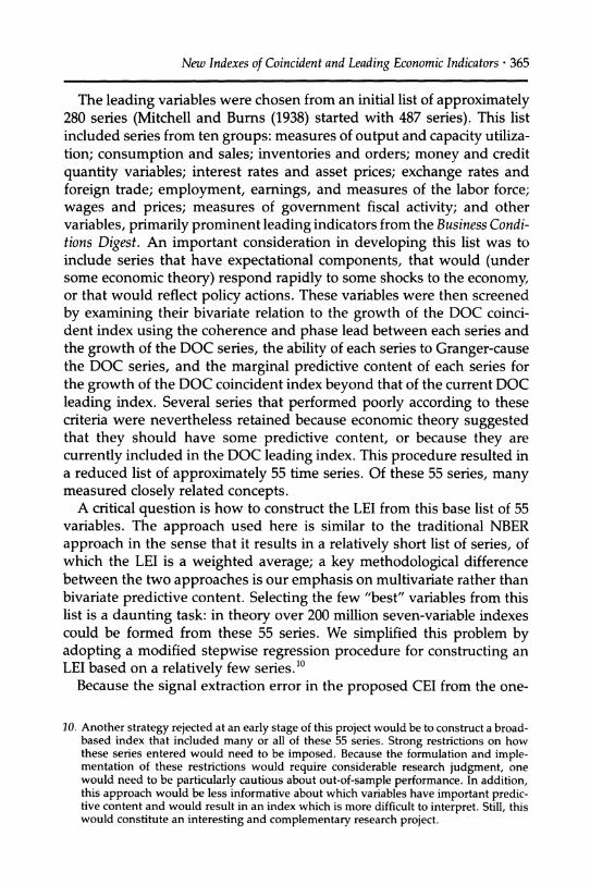
The leading variables were chosen from an initial list of approximately 280 series (Mitchell and Burns (1938) started with 487 series). This list included series from ten groups: measures of output and capacity utiliza- tion; consumption and sales; inventories and orders; money and credit
quantity variables; interest rates and asset prices; exchange rates and
foreign trade; employment, earnings, and measures of the labor force; wages and prices; measures of government fiscal activity; and other variables, primarily prominent leading indicators from the Business Condi- tions Digest. An important consideration in developing this list was to include series that have expectational components, that would (under some economic theory) respond rapidly to some shocks to the economy, or that would reflect policy actions. These variables were then screened
by examining their bivariate relation to the growth of the DOC coinci- dent index using the coherence and phase lead between each series and the growth of the DOC series, the ability of each series to Granger-cause the DOC series, and the marginal predictive content of each series for the growth of the DOC coincident index beyond that of the current DOC
leading index. Several series that performed poorly according to these criteria were nevertheless retained because economic theory suggested that they should have some predictive content, or because they are
currently included in the DOC leading index. This procedure resulted in a reduced list of approximately 55 time series. Of these 55 series, many measured closely related concepts.
A critical question is how to construct the LEI from this base list of 55 variables. The approach used here is similar to the traditional NBER approach in the sense that it results in a relatively short list of series, of which the LEI is a weighted average; a key methodological difference between the two approaches is our emphasis on multivariate rather than bivariate predictive content. Selecting the few "best" variables from this list is a daunting task: in theory over 200 million seven-variable indexes could be formed from these 55 series. We simplified this problem by adopting a modified stepwise regression procedure for constructing an LEI based on a relatively few series.10
Because the signal extraction error in the proposed CEI from the one-
10. Another strategy rejected at an early stage of this project would be to construct a broad- based index that included many or all of these 55 series. Strong restrictions on how these series entered would need to be imposed. Because the formulation and imple- mentation of these restrictions would require considerable research judgment, one would need to be particularly cautious about out-of-sample performance. In addition, this approach would be less informative about which variables have important predic- tive content and would result in an index which is more difficult to interpret. Still, this would constitute an interesting and complementary research project.

366 * STOCK & WATSON
Figure 4 A. THE PROPOSED INDEX OF COINCIDENT INDICATORS (SOLID LINE) AND THE CURRENT DOC INDEX OF COINCIDENT ECONOMIC INDICATORS (DASHED LINE)
0
~I? I ~ o
( 60 62 64 66 68 70 72 74 76 78 80 82 84 86 88
factor model is relatively small, an LEI produced using the unobserved- components VAR can be approximated by regressing the six-month growth in the CEI (Ct+61t+6-Ctlt) on current and past values of the candidate leading variables. This observation was used to construct several leading indexes. Starting with a base set of series, indexes were constructed by including twelve lags of each of the candidate trial variables in the six-step ahead regression; these were ranked according to a criterion that involved the full-sample R2 and the R2 based on the full-sample performance of the index when the model was estimated through 1979:9. The series with the greatest value of the criterion function was added to the index, and the procedure was repeated until the desired number of variables was added. The series proposed in Table 1 were obtained by considering those series that most often were found in the final index, starting from different sets of base variables. In addition, judgment was used in excluding some variables that were clearly fitting specific historical episodes in a way that had no plausible economic interpretation (a sign of overfitting).
indexes. Starting with a base set of ser
60 6 2 64 66 68 70 72 74 76 78 80 82 84 86 88
factor model is relatively small, an LEI produced using the unobserved- components VAR ca n be approximated by regressing the six-month growth in the CEI (Ct +6esi6-Ctjt) o n current and past values of th e candidate leading variables. This observation was used to construct several leading indexes. Starting with a base set of ser ies, indexes w ere constructed by including twelve lags of each of the candidate trial variables in the six-step ahead regression; th ese were ranked according to a criterion that involved
had no plausible economic interpretation (a sign of overfitting).
New Indexes of Coincident and Leading Economic Indicators * 367
Because the growth rates of some of the series contain considerable
high frequency noise, some of the series were smoothed. Although this
smoothing could in principle be done implicitly by estimating a larger number of regression coefficients, using smoothed series admits the
possibility of reducing the number of estimated regression coefficients. The smoothing filter was chosen to be s(L) = 1+2L+2L2+L3, the filter used by the DOC (until the 1989 revision) to smooth several of their
noisy series. This filter has desirable properties from the perspective of
producing six-month ahead forecasts using first differences of leading variables. The product filter (1-L)s(L) is a band-pass filter with gain concentrated at periods of four months to one year, zero gain at zero
frequency and very low gain for periods less than two months. At a
period of six months, the phase lag of this filter is 2.5 months. The number of lags of each series in the ACt equation of the LEI model
(i.e., the order of Acy(L) in (4)) was chosen using the Akaike information criterion (AIC) in a regression of ACtlt on four lags of ACt,t and the selected
leading variables. The search was restricted to models with 1, 3, 6, or 9
lags of the variables for computational reasons." Various tests for auto-
regressive order resulted in setting the orders of Acc(L), yyc(L), and yy(L) at 4, 1, and 1 respectively. The AIC calculations resulted in a model with six
lags of housing starts and the private-public spread and with three lags of each of the other variables. The within-sample R2 between the resultant LEI and the actual six-month growth of the proposed CEI is .634.
Overfitting the data (and the consequent poor out-of-sample perfor- mance) is a risk in any empirical exercise, and the danger is particularly clear here. The first potential source of overfitting-the selection of a final list of leading variables from a much longer list of series-is present both in our procedure and in the traditional NBER/DOC procedure for variable selection (see Zarnowitz and Boschan 1975a,b and Moore 1988). The DOC
periodically sponsors a revision of the composite indexes; one interpreta- tion of the need for these revisions is that the underlying relations (and important predictive variables) have changed in the economy, but another is that these revisions are important to correct for previous overfitting.12 The methodology outlined above introduces a second possible source of
overfitting, the estimation of regression coefficients.
11. This entailed examining 47 specifications. The AIC is known to overestimate the autoregression order if the order is finite (e.g., Geweke and Meese 1981). As a check, lags were chosen according to the Schwartz information criterion (BIC) and the Hannan-Quinn information criterion. These yielded similar choices of lag lengths, and in particular yielded similar estimated LEIs.
12. Recent revisions occurred in 1975 and 1983. A new set of revisions took effect with the January 1989 data. See Hertzberg and Beckman (1989).
368 * STOCK & WATSON
It appears difficult to ascertain the asymptotic properties of this model selection procedure, but these properties can be investigated numeri-
cally. Two small Monte Carlo experiments were performed to shed light on the potential overfitting. The first simulated indexes that would be
produced if no series had any true predictive content for the CEI. Fifty smoothed pseudo-random monthly time series of the form xit = s(L)eit, Eit i.i.d. N(0,1) were generated for i = 1, . . ., 50, t = 1959:1, . . ., 1987:12. The variable and model selection procedure described above was then
applied to these time series, and the resultant seven-variable index was calculated. This experiment was repeated twice, and resulted in indexes with R2,s of .228 and .271. The R2 for a model with no leading variables is .163 over this period (this is non-zero because lagged growth of Ctlt predicts its future growth); thus the increment to the R2 in these Monte Carlo experiments was respectively .065 and .108.
The second Monte Carlo experiment examined a situation where most of the variables have some predictive content, but the chosen series might not be those with the greatest true predictive ability. The estimated seven- variable leading model (4) and (5) was used to generate seven Gaussian
pseudo-random leading variables over 1959:1-1987:12, plus a pseudo- random coincident index. For each of the seven pseudo-random leading variables, four more pseudo-random series were constructed by adding various degrees of measurement error to series.13 Fifteen additional smoothed spurious series like those used in the first experiment were also
generated, for a total of fifty pseudo-random potential leading series. The variable and model selection procedure was then used to produce a seven-variable index. The population R2 for the model generating the data was .65. The average Monte Carlo R2 of the chosen models across ten
replications was .75, and these (suboptimal) models had an average popu- lation R2 of .62. Thus imperfect knowledge of the correct model reduced the R2 by .03 (.65- .62). Also, on average the sample R2,s were inflated by .13 (.75-.62) above their population counterparts.
These two experiments provide rough measures of the magnitude of the overfitting bias: in the first, approximately .08, in the second, .13.14
13. For each of the base pseudo-random leading series Xit, i = 1, .. . ,7, the four additional pseudo-random series were constructed by settins Xijt = Fj(L)Xit+uijt, where u,, are i.i.d. N(0,72) random variables, Fj(L) = 1, 1, L, and L , and r = 1, 5, 1, and 1 forj = 1, 2, 3, and 4, respectively.
14. One reason to suspect that these experiments overstate the bias is that they do not incorporate any researcher judgment, although the construction of the proposed LEI did. In addition, the first experiment fails to recognize that the 55 actual series have many closely related variables (e.g., industrial production of consumer durables and industrial production in manufacturing); thus in actuality the variation across the series is not as great as in the first experiment.

New Indexes of Coincident and Leading Economic Indicators ? 369
The experimental LEI and its Historical Components. Historical values of the proposed LEI are plotted in Figure 2. A negative value of the index indicates a forecast of negative growth in overall economic conditions over the next six months. This index is negative prior to each of the four recessions since 1960. It is also negative during 1967, a year in which a recession did not occur.
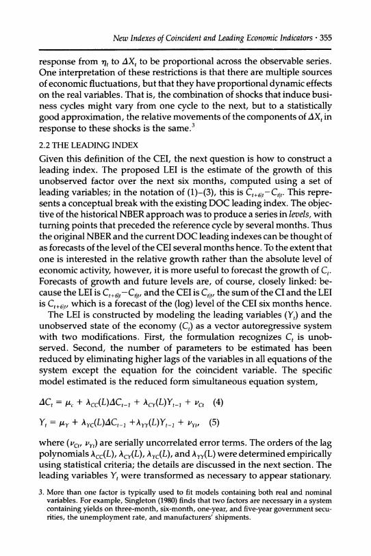
The historical contributions of each of the seven leading variables to the index are plotted in Figure 5. These historical contributions are calcu- lated by setting all series but the series in question to zero, then comput-
Figure 5 HISTORICAL DECOMPOSITION OF THE PROPOSED LEI (A) Total
In
I -I
0
v - I II I I I I I I I I I ._1
60 62 64 66 68 70 72 74 76 78 80 82 84 86 88
(B) COMPONENT DUE TO HSBP
?O I '.1 . I IV IV L Ojr ur l trl
I ri
oj if o I
t_- I I I I I 1 I - I A !I I I I I I I
60 62 64 66 68 70 72 74 76 78 80 82 84 86 88

370 * STOCK & WATSON
Figure 5 (CONTINUED) (C) COMPONENT DUE TO MDU82S
0
LO .__ _____ If
.JiJ A -II ,: lOIh t
I .'1%.1 ? a ~l " 1 I, [
-II o -
Ig 0 II
1 60 62 64 66 68 70 72 74 76 78 80 82 1
(D) COMPONENT DUE TO EXNWT2S
0
34 86 88
1 60 62 64 66 68 70 72 74 76 78 80 82 84 86 88
ing the LEI. Because the LEI is linear in Yt, the sum of these historical
decompositions, plus the mean six-month growth in the CEI (at annual rates), equals the LEI (graphed again in Figure 5(a) for convenience).15
15. Readers familiar with vector autoregressions (VARs) should not confuse the historical decompositions in Figure 5 with those found in the VAR literature for "orthogonalized" systems. The latter are based on an arbitrary transformation of the original linear model (chosen so that the shocks to each decomposition are mutually uncorrelated), whereas no such transformation is made in producing Figure 5.
New Indexes of Coincident and Leading Economic Indicators * 371
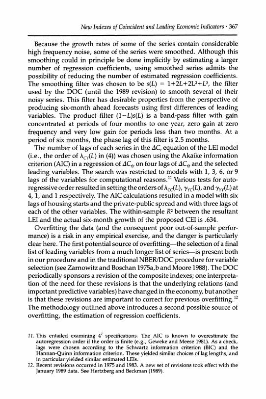
Figure 5 (CONTINUED) (E) COMPONENT DUE TO LHNAPSS
0 1-
1 60 62 64 66 68 70 72 74 76 78 80 82 84 86 88
(F) COMPONENT DUE TO FYGT10
0
o
o
LO
I
0o
i) I
60 62 64 66 68 70 72 74 76 78 80 82 84 86 88
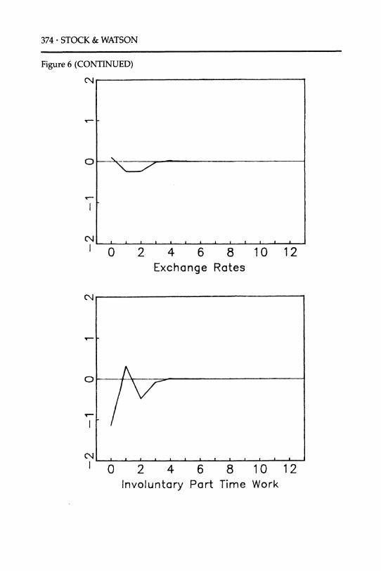
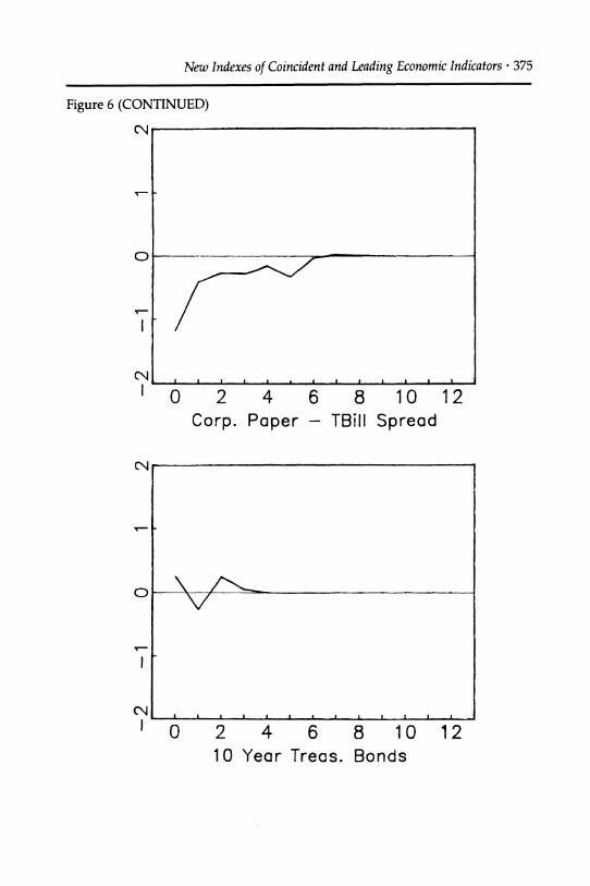
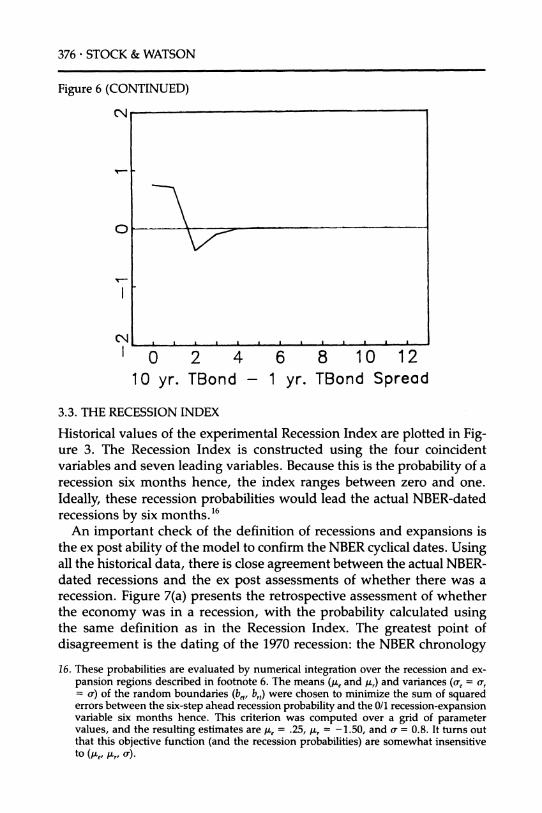
The implicit weights on the variables used to construct the LEI (the implied "distributed lag" coefficients) are plotted in Figure 6; the units are standard deviations of the leading variables.
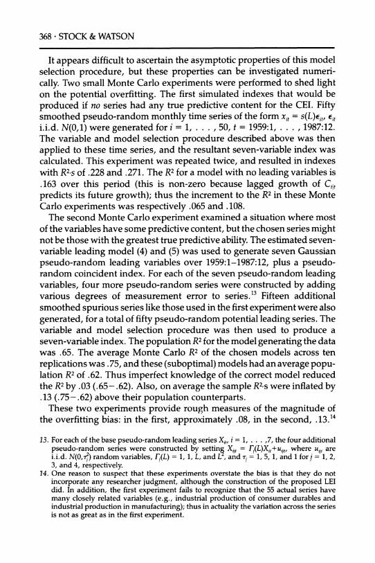
Each of the series makes a contribution to the total. The largest histori- cal contributions are from the spread between commercial paper and Treasury bills, from the spread between the yields to maturity on 10-year and 1-year Treasury Bonds, from housing starts, from manufacturer's unfilled orders in durable goods industries, and from the growth of part-
372 * STOCK & WATSON
Figure 5 (G) COMPONENT DUE TO CP6_ GM6 (CONTINUED)
Ln * * ** * * I . I I L
~~I~~~~~f)~ I
I 1 I I !t J 1 I I I I J I I I I I I
I 60 62 64 66 68 70 72 74 76 78 80 82 84 86 88
(H) COMPONENT DUE TO G10 _ G
....,,. ,. , , 1, , ,, ,, , 1, ', ? I II J
J
I-I I I I a
.
Ii I I I __
1 60 62 64 66 68 70 72 74 76 78 80 82 84 86 88
time work due to "slack work." The implied distributed lag coefficients indicate that a rise in housing starts, a low private-public spread, a high long-term/short-term public spread (an upward-sloping yield curve), an increase in durables manufacturers' unfilled orders, and a decline in
involuntary part-time work all are indications of strong overall growth over the next six months. To a lesser extent, a depreciation of the dollar and an increase in the long-term Treasury bond yield signify strong future economic activity.
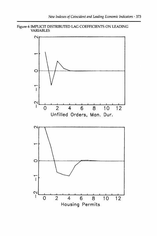
New Indexes of Coincident and Leading Economic Indicators ? 373
Figure 6 IMPLICIT DISTRIBUTED LAG COEFFICIENTS ON LEADING VARIABLES
CN
0C
0 2 4 6 8 10 12 Unfilled Orders, Man. Dur.
C \
0
C\ a i i , a a I i . I a a
0 2 4 6 8 10 12 Housing Permits
374 * STOCK & WATSON
Figure 6 (CONTINUED)
CN
\ ---
N , I 0 2
I I i I I I i I
4 6 8 10 12 Exchange Rates
I 0 2 4 6 8 10 12 Involuntary Part Time Work
New Indexes of Coincident and Leading Economic Indicators * 375
Figure 6 (CONTINUED) (i\i
0
N ! I a i I I I I I I I
0 2 Corp.
4 Paper
6 8 TBill
10 Spread
12
LN
t'I-
CN , I I I I I I I I I a
0 2 4 6 8 1C 10 Year Treas. Bonds
) 12 I
376 * STOCK & WATSON
Figure 6 (CONTINUED)
C'
C\\
I'
I 0 .2 4 6 8 . 1 0 2 4 6 8 10 12 10 yr. TBond - 1 yr. TBond Spread
3.3. THE RECESSION INDEX
Historical values of the experimental Recession Index are plotted in Fig- ure 3. The Recession Index is constructed using the four coincident variables and seven leading variables. Because this is the probability of a recession six months hence, the index ranges between zero and one.
Ideally, these recession probabilities would lead the actual NBER-dated recessions by six months.16
An important check of the definition of recessions and expansions is the ex post ability of the model to confirm the NBER cyclical dates. Using all the historical data, there is close agreement between the actual NBER- dated recessions and the ex post assessments of whether there was a recession. Figure 7(a) presents the retrospective assessment of whether the economy was in a recession, with the probability calculated using the same definition as in the Recession Index. The greatest point of
disagreement is the dating of the 1970 recession: the NBER chronology
16. These probabilities are evaluated by numerical integration over the recession and ex- pansion regions described in footnote 6. The means (Ae and /,) and variances (o-, = a, = o) of the random boundaries (b,, brt) were chosen to minimize the sum of squared errors between the six-step ahead recession probability and the 0/1 recession-expansion variable six months hence. This criterion was computed over a grid of parameter values, and the resulting estimates are AL = .25, L, = -1.50, and c = 0.8. It turns out that this objective function (and the recession probabilities) are somewhat insensitive to (L,e /Ar, a).
New Indexes of Coincident and Leading Economic Indicators ? 377
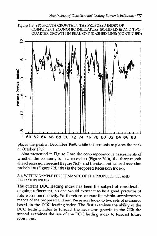
Figure 6 B. SIX-MONTH GROWTH IN THE PROPOSED INDEX OF COINCIDENT ECONOMIC INDICATORS (SOLID LINE) AND TWO- QUARTER GROWTH IN REAL GNP (DASHED LINE) (CONTINUED)
CL IvWj ;Al 14\, I
CO
O *
_ III I I1
* I I I I I I ..I .1. . Ii t
1 60 62 64 66 68 70 72 74 76 78 80 82 84 86 88
places the peak at December 1969, while this procedure places the peak at October 1969.
Also presented in Figure 7 are the contemporaneous assessments of whether the economy is in a recession (Figure 7(b)), the three-month ahead recession forecast (Figure 7(c)), and the six-month ahead recession probability (Figure 7(d); this is the proposed Recession Index).
3.4. WITHIN-SAMPLE PERFORMANCE OF THE PROPOSED LEI AND RECESSION INDEX
The current DOC leading index has been the subject of considerable ongoing refinement, so one would expect it to be a good predictor of future economic activity. We therefore compare the within-sample perfor- mance of the proposed LEI and Recession Index to two sets of measures based on the DOC leading index. The first examines the ability of the DOC leading index to forecast the near-term growth in the CEI; the second examines the use of the DOC leading index to forecast future recessions.

378 * STOCK & WATSON
Figure 7 RECESSION PROBABILITIES: (A) EX POST
0
00 d
o c It d
ON d
c d 62 64 66 68 70 72 74 76 78 80 82 84 86 88
(B) CONTEMPORANEOUS
0
o d
d
c:t
d
I F 7
~~~~I
a- .. . A I IJ. . f I , .fl I El I I I , I l I I Al I i- Li -ij o 62 64 66 68 70 72 74 76 78 80 82 84 86 88
Forecasts of Growth. The within-sample fit of the proposed LEI is gener- ally good. The within-sample R2 between the LEI and the true six-month growth of the CEI (Ct+6t+6t-Ctlt) is .634 over 1961:1-1988:4. The LEI and the actual six-month growth of the CEI are plotted in Figure 8(a). The most noteworthy within-sample errors occurred in the middle of the 1982 recession: the LEI was predicting approximately zero growth, while the actual growth turned out to be sharply negative.
Because the six-month growth of the CEI is highly correlated with the two-quarter growth of GNP, one way to measure performance is to com-
I I'
'
I 0
I
a! I I I ? A I a
I
a j - ? i I a
I
New Indexes of Coincident and Leading Economic Indicators * 379
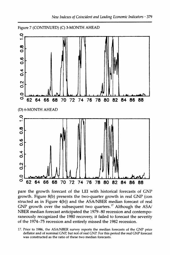
Figure 7 (CONTINUED) (C) 3-MONTH AHEAD
0 e-
0 62 64 66 68 70 72 74 76 78 80 82 84 86 88
(D) 6-MONTH AHEAD
62 64 66 68 70 72 74 76 78 80 82 84 86 88
pare the growth forecast of the LEI with historical forecasts of GNP
growth. Figure 8(b) presents the two-quarter growth in real GNP (con structed as in Figure 4(b)) and the ASA/NBER median forecast of real GNP growth over the subsequent two quarters.17 Although the ASA/ NBER median forecast anticipated the 1979-80 recession and contempo- raneously recognized the 1980 recovery, it failed to forecast the severity of the 1974-75 recession and entirely missed the 1982 recession.
17. Prior to 1986, the ASA/NBER survey reports the median forecasts of the GNP price deflator and of nominal GNP, but not of real GNP. For this period the real GNP forecast was constructed as the ratio of these two median forecasts.
380 * STOCK & WATSON
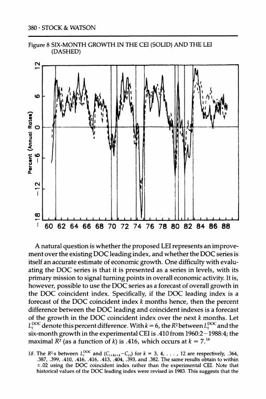
Figure 8 SIX-MONTH GROWTH IN THE CEI (SOLID) AND THE LEI (DASHED)
I'
,O I I i t I I)I'?
I~ lr 1
w - I i
r 1 II fl. I C
0~pL.UC4' fiit
00
I 60 62 64 66 68 70 72 74 76 78 80 82 84 86 88
A natural question is whether the proposed LEI represents an improve- ment over the existing DOC leading index, and whether the DOC series is itself an accurate estimate of economic growth. One difficulty with evalu-
ating the DOC series is that it is presented as a series in levels, with its
primary mission to signal turning points in overall economic activity. It is, however, possible to use the DOC series as a forecast of overall growth in the DOC coincident index. Specifically, if the DOC leading index is a forecast of the DOC coincident index k months hence, then the percent difference between the DOC leading and coincident indexes is a forecast of the growth in the DOC coincident index over the next k months. Let LDC denote this percent difference. With k = 6, the R2between LDOC and the six-month growth in the experimental CEI is .410 from 1960:2-1988:4; the maximal R2 (as a function of k) is .416, which occurs at k = 7.18
18. The R2,s between LtDC and (Ct+ktt+k-Ctlt) for k = 3, 4, .. ., 12 are respectively, .364, .387, .399, .410, .416, .416, .413, .404, .393, and .382. The same results obtain to within +.02 using the DOC coincident index rather than the experimental CEI. Note that historical values of the DOC leading index were revised in 1983. This suggests that the
New Indexes of Coincident and Leading Economic Indicators * 381
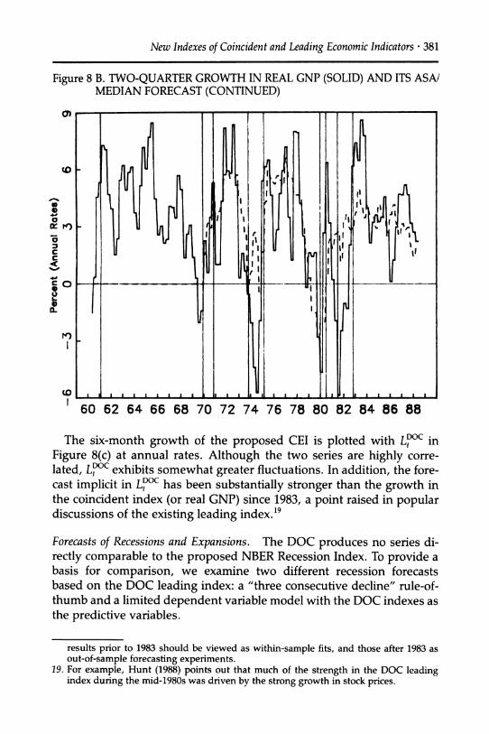
Figure 8 B. TWO-QUARTER GROWTH IN REAL GNP (SOLID) AND ITS ASA/ MEDIAN FORECAST (CONTINUED)
C) -
I
to - J
LJ. I I
i1 606 6 677 c 1 ' 1i ,'n i c 1 I 'ol I I
60 62 64 66 68 70 72 74 76 78 80 82 84 86 88
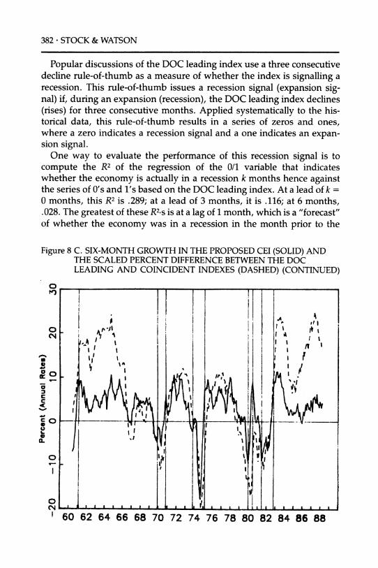
The six-month growth of the proposed CEI is plotted with LDOC in Figure 8(c) at annual rates. Although the two series are highly corre- lated, L?C exhibits somewhat greater fluctuations. In addition, the fore- cast implicit in L?C has been substantially stronger than the growth in the coincident index (or real GNP) since 1983, a point raised in popular discussions of the existing leading index.19
Forecasts of Recessions and Expansions. The DOC produces no series di- rectly comparable to the proposed NBER Recession Index. To provide a basis for comparison, we examine two different recession forecasts based on the DOC leading index: a "three consecutive decline" rule-of- thumb and a limited dependent variable model with the DOC indexes as the predictive variables.
results prior to 1983 should be viewed as within-sample fits, and those after 1983 as out-of-sample forecasting experiments.
19. For example, Hunt (1988) points out that much of the strength in the DOC leading index during the mid-1980s was driven by the strong growth in stock prices.
382 * STOCK & WATSON
Popular discussions of the DOC leading index use a three consecutive decline rule-of-thumb as a measure of whether the index is signalling a recession. This rule-of-thumb issues a recession signal (expansion sig- nal) if, during an expansion (recession), the DOC leading index declines (rises) for three consecutive months. Applied systematically to the his- torical data, this rule-of-thumb results in a series of zeros and ones, where a zero indicates a recession signal and a one indicates an expan- sion signal.
One way to evaluate the performance of this recession signal is to compute the R2 of the regression of the 0/1 variable that indicates whether the economy is actually in a recession k months hence against the series of 0's and l's based on the DOC leading index. At a lead of k = 0 months, this R2 is .289; at a lead of 3 months, it is .116; at 6 months, .028. The greatest of these R2,s s at a lag of 1 month, which is a "forecast" of whether the economy was in a recession in the month prior to the
Figure 8 C. SIX-MONTH GROWTH IN THE PROPOSED CEI (SOLID) AND THE SCALED PERCENT DIFFERENCE BETWEEN THE DOC LEADING AND COINCIDENT INDEXES (DASHED) (CONTINUED)
0 P3
0-s a
0
C c
c4
C 0
0 a.
New Indexes of Coincident and Leading Economic Indicators * 383
most recent month for which there are data. In contrast, the R2 for the series in Figure 7(b)-7(d) are respectively .88 at 0 months lead, .64 at a lead of 3 months, and (for the proposed Recession Index) .50 at a lead of 6 months.
Although this rule-of-thumb is commonly used to forecast recessions, it is probably not the most efficient use of the information contained in the DOC index. As an additional comparison, logit models were esti- mated with the true 0/1 recession indicator six months hence as the
dependent variable and with, alternately, lags of LD?c and of the growth of the DOC leading index as predictive variables. The greatest of the
resulting R2 s was .292, which obtained in a logit model with eight lags of LD?c as the predictive variables.
In summary, these historical comparisons suggest that the proposed LEI and Recession Index are potentially substantial improvements over the existing indexes, both in performance and in ease of interpretation. Whether this potential is realized will, of course, depend on the future behavior of the indexes.
4. Interpretation and Discussion
The construction of the experimental LEI systematically focused on find-
ing a set of macroeconomic variables that jointly have the ability to forecast future economic activity in a reduced-form model. This section examines the resulting index and its components from the perspective of macroeconomic theory.
4.1. DISCUSSION OF VARIABLES INCLUDED IN THE LEI
Long-term/short term treasury bond yield spread. One of the novel features of the experimental LEI is its use of interest rate spreads as macro- economic predictors. It is generally recognized that a declining yield curve signals a future slowdown in economic activity. The 10-year/I-year Treasury bond spread became negative in 1959, 1966, 1973, 1978, and 1981; with the exception of 1966, each of these inversions in the yield curve preceded an NBER-dated cyclical peak by approximately one year. Similarly, five of the seven cessations of the inversion over this period preceded a cyclical trough by approximately six months to one year. Recent work in financial econometrics has produced the intriguing re- lated result that measures of the slope of the yield curve are useful predictors of a variety of financial variables. For example, Campbell (1987) and Fama and French (1989) document that measures of the slope

384 * STOCK & WATSON
of the term structure at short horizons have predictive content for excess returns on a variety of assets.20
These observations are consistent with a macroeconomic theory in which real rates are temporarily high, perhaps because of tight monetary policy, which in turn results in a postponement of investment and a decline in future activity. Additionally, if market participants expect fu- ture growth to be low and believe a Phillips relation to hold, then inflation would be expected to drop and the yield curve would tend to invert. Thus this predictive content is consistent with a theory in which monetary policy works through interest rates and in which inflation and output growth are positively related. It seems to be more difficult to reconcile this
finding with a simple real business cycle model in which the marginal product of capital equals the interest rate and in which persistent produc- tivity shocks drive the business cycle: in this case, a positive productivity shock would result in a high marginal product of capital that is expected to decline over time as investment (and output) increases.
Private-public interest rate spread. Although the average spread from 1959 to 1988 is only 60 basis points, during and preceding the 1970 and 1980 recessions it exceeded 150 basis points, and during 1975 it rose to over 350 basis points. The predictive power of similar spreads has been documented by Bernanke (1983), who showed that the Baa-Treasury bond spread forecasted industrial production in the interwar period, and
by Friedman and Kuttner (1989), who (independently) concluded that the corporate paper-Treasury bill spread has strong predictive power for industrial production over the period considered here. Like the slope of the yield curve, the private-public spread has recently been recognized as a predictor of various asset returns. Keim and Stambaugh (1986) find that monthly risk premiums on a variety of bonds can be explained with some success by the spread between the yield on long-term low-grade corporate paper and short-term Treasury bills (note however that the maturities in this spread are not matched).
One interpretation of these results is that the private-public spread measures the default risk on private debt. If private lenders can accu-
rately assess increased default risks for individual firms or industries, these changes will, after aggregation, be reflected as increases in the
spread. Thus the spread could serve as a useful aggregator of informa-
20. In related research, Knez, Litterman, and Scheinkman (1989) identify three common systematic risk factors underlying a variety of money market returns. They associate these factors with shifts in the yield curve, tilts in the yield curve, and changes in the public-private spread. Thus the three factors correspond closely to the three interest rate measures in the proposed LEI.

New Indexes of Coincident and Leading Economic Indicators * 385
tion about the prospects of private firms, known best by those buying and selling the debt of those firms. An alternative interpretation would emphasize the allocative role of interest rates: an increase in the spread, all else equal, might induce some firms to postpone investment, result- ing in a decline in aggregate demand.
Change in the 10-year Treasury bond yield. Previous research on the predic- tive content of various financial and monetary variables has emphasized the importance of interest rates or their changes (e.g., Sims 1980), so it is not surprising that changes in the long-term public bond rate have some forecasting content. Interestingly, including a measure of ex ante real rates (with various measures of expected inflation) does not improve the performance of the LEI. In fact, simulated out-of-sample experiments indicate that including a real rate would have dramatically worsened substantially the performance during the 1980s because of the histori- cally high real rates since 1982.
Trade-weighted nominal exchange rate. A depreciation of the dollar rela- tive to the currencies of its major trading partners makes a small positive contribution to the LEI. The sign and the magnitude are consistent with the depreciation being associated with a modest subsequent increase in net demand for domestically produced goods relative to foreign goods.
Part-time work in nonagricultural industries (slack work). An increase in slack work results in a substantial drop in the LEI, holding the compo- nents constant. This measure is closely related to indicators in the current DOC index (new claims for unemployment insurance and the average weekly hours of production workers in manufacturing); the procedure described in the previous section indicates that part-time work has pref- erable statistical properties compared with these other indicators. One interpretation of the predictive value of this series is that the initial re- sponse of some firms to productivity and demand shocks is not just to adjust inventories, but to vary labor input. In addition, this is measured better by part-time employment than by layoffs or by average hours.
Housing authorizations. This series, currently in the DOC leading index, could play several roles. Private housing is the most durable of con- sumer goods. Thus movements in housing authorizations could be a proxy for broader changes in demand for consumer durables, perhaps in response to movements in interest rates or to fluctuations in (the present value of) aggregate income. In addition, changes in housing authoriza- tions could signal more widespread changes in future activity in the
386 * STOCK & WATSON
construction sector which, to the extent that there is a multiplier mecha- nism, might spill over into other sectors of the economy.
Manufacturers' unfilled orders (durable goods industries). The DOC has (in- dependently) decided to include manufacturer's unfilled orders in dura- ble goods industries in the revised DOC leading index starting in Janu- ary 1989. Unfilled orders are much like negative inventories, and can be used (like inventories) to minimize production costs over time. Thus unfilled orders can be expected to increase in response to unexpected increases in demand or to temporary increases in production costs. The time series properties of unfilled orders will depend on the extent of
production smoothing, production times, the relative mix of demand and supply shocks, and the lead-lag relation between new orders for durables and aggregate activity.
B. DISCUSSION OF SELECTED VARIABLES EXCLUDED FROM THE LEADING INDEX
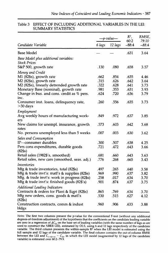
The proposed LEI excludes some variables that appear in the current DOC index or which economic theory suggests could have important predictive power. Summary statistics for the effect of including several such series in the LEI are presented in Table 3. The first column presents the p-value for the F-test of the restriction that the coefficients on lags of the candidate additional leading variable are zero in a regression of the one-month growth of the CEI on the variables in the LEI and on six lags of the candidate variable. The second column contains the same statistic, except that 12 lags of the candidate variable are included in the regres- sion. The third column contains the within-sample R2 between the six- month growth of the CEI and the LEI, constructed using the base vari- ables and lags described in Section 3 and 12 lags of the candidate vari- able. The fourth column contains the out-of-sample root mean square error from October 1979 to April 1988 based on an LEI model estimated
through September 1979.21
Stock Prices. The present value theory of stock prices implies that move- ments in the stock market reflect changing expectations of future earn-
21. As a simplification, columns 3 and 4 of Table 3 are based on LEI models that were estimated using a conventional multivariate regression specified with Ctlt, Yt and the candidate leading variable. That is, Ct was not treated as unobserved as in the estima- tion of the LEI in Section 3, but rather was replaced by C,it. Now specified in terms of observables, the system was esimated by OLS equation by equation. The numerical error that arises from this simplification is slight because of the small signal extraction in Ctlt.
New Indexes of Coincident and Leading Economic Indicators * 387
Table 3 EFFECT OF INCLUDING ADDITIONAL VARIABLES IN THE LEI: SUMMARY STATISTICS
.~ ~ ~ 2 ME
Candidate Variable
- p-value- R2, RMSE, - -la 1lu- 60:2 79:10
6 lags 12 lags -88:4 -88:4
Base Model Base Model plus additional variables: Stock Prices S&P 500, growth rate
Money and Credit M1 (82$s), growth rate M2 (82$s), growth rate M2 (82$s), linearly detrended growth rate Monetary Base (nominal), growth rate Change in bus. and cons. credit as % pers. inc. Consumer inst. loans, delinquency rate, >30 days Employment Avg weekly hours of manufacturing work- ers New claims for unempl. insurance, growth rates No. persons unemployed less than 5 weeks Sales and Consumption IP-consumer durables Pers cons expenditures, durable goods (82$s) Retail sales (1982$'s, smoothed) Retail sales, new cars (smoothed, seas. adj.) Inventories Mfg & trade inventories, total (82$s) Mfg & trade invt's: matl's & supplies (82$s) Mfg. & trade invt's: work in progress (82$s) Mfg & trade invt's: finished goods (82$'s) Additional Leading Indicators Contracts & orders for Plant & Eqpt (82$s) Mfg new orders, cons. goods & matl's (82$s) Construction contracts, comm & indust bldgs
.631 3.64
.130 .080
.662 .854
.315 .626
.322 .628
.981 .353
.624 .720
.260 .556
.658 3.57
.635
.642
.641
.631
.636
4.46 3.64 3.73 3.93 3.79
.635 3.73
.849 .972 .637 3.85
.573 .603
.007 .003
.300 .507
.721 .472
.681 .660
.776 .268
.497 .265
.969 .990
.258 .017
.901 .874
.865 .769
.530 .515
.642 3.68
.630 3.62
.638 4.25
.643 3.66
.643 3.63
.665 3.43
.640
.637
.634
.637
3.58 3.82 3.70 3.75
.634 3.70
.627 4.12
.960 .906 .633 3.88
Notes: The first two columns present the p-value for the conventional F-test (without any additional degrees-of-freedom adjustment) of the hypothesis that the coefficients on the candidate leading variable are zero in a regression of ACtlt on the base set of leading variables (with the same number of lags as are used to construct the NBER LEI), estimated by OLS, using 6 and 12 lags respectively of the candidate variable. The third column presents the within-sample R2 when the LEI model is estimated using the full sample and 12 lags of the candidate variable. The final column contains the out-of-column RMSE between the LEI and Ct+6t+6 - Ct, in which the LEI model (augmented by 12 lags of the candidate variable) is estimated over 60:2-79:9.
388 * STOCK & WATSON
ings of publicly traded corporations. Additional theoretical links from the stock market to future economic activity come through the role of stock prices as a determinant of the cost of capital (q-theory) and through wealth effects on consumption. Stock prices therefore ought to be an indicator of future growth, and indeed were identified as leading indica- tors by Mitchell and Burns (1938). Fama (1981) and Fisher and Merton
(1984) document the substantial predictive value of stock prices for out-
put. As they do for GNP at longer horizons, stock prices have strong predictive content for the growth in the CEI; the R2 of a regression of
Ct+6lt+6 -Ctt on 12 lags of the growth in the Standard and Poor's 500 is .318, and the hypothesis that the growth of the S&P 500 does not Granger- cause ACtlt can be rejected at the .5% significance level.
A result from this research is that the marginal predictive content of stock prices for the six-month growth in the CEI is modest. As reported in Table 3, the hypothesis that stock prices have no marginal (linear) predictive content for ACt,I cannot be rejected at the 5% level.22 Although the R2 for the six-step ahead forecast increases somewhat when S&P 500
growth is included, this specification increases the number of estimated
parameters in the AC,tl equation from 28 to 40. Although there is some evidence that the stock market improves forecasting performance, this
improvement is slight. These findings are consistent with a view that, from the perspective of forecasting, the expectational aspect of the stock market dominates its allocative role, and that these expectations can be
captured by examining other variables.
Money and Credit. The marginal predictive content of money for output is one of the most studied relations in empirical macroeconomics; see Christiano and Ljungqvist (1988) and Stock and Watson (1989) for recent results and reviews of the literature. A primary focus of this literature has been whether the predictive content of money growth in a bivariate
system is eliminated by including an interest rate. The proposed LEI
provides an opportunity to examine the marginal predictive content of
money in a system with measures of real activity and, notably, with a richer set of interest rates.
The predictive content of real M2 growth in a bivariate system with
ACtI, is substantial: Granger non-causality can be rejected at the 0.5% level, and the R2 of the regression of Ct+61t+6-Ctlt onto 12 lags of real M2 is .435. As the results in Table 3 indicate, however, on the margin real M1, real M2, and the monetary base add nothing to the forecasting ability of
22. The large number of variables involved in the search suggests skepticism about the use of the usual asymptotic distributions for these test statistics. An informal way to correct for this is to use a more conservative critical value than usual, say 1%.
New Indexes of Coincident and Leading Economic Indicators ? 389
the LEI. The simulated out-of-sample performance of the index includ-
ing M1 deteriorates substantially, indicating parameter instability. These results hold using either the growth rate of M2 or, as suggested by Stock and Watson (1989), the detrended growth rate.
These findings are consistent with several hypotheses. Friedman (1988) argues that even if money had predictive content during earlier
periods, its reduced-form relation to output has changed (or vanished) as a result of financial deregulation. This is consistent with the observa- tion that the economy has performed well in the last two years despite the absolute decline of real M2 between October 1986 and October 1988.
Alternatively, the inclusion of interest rate spreads (in particular the
yield curve) might be a more sensitive measure to monetary intervention than is the interest rate alone, the variable typically examined by other authors.
Measures of the quantity of credit have also received some attention as
possible predictive variables. The change in business and consumer credit appears in the current DOC leading index; scaled to be a percent of personal income rather than in nominal dollars, this change has no
statistically significant predictive content.
Employment. The DOC leading index contains two employment series not in the proposed LEI: average weekly hours of manufacturing work- ers and new claims for unemployment insurance. Neither make an im- portant marginal contribution to the proposed LEI.23 While the number of individuals unemployed less than five weeks is a statistically signifi- cant predictor of ACtlt at the 5% level, the six-month ahead forecast is not improved by including it in the index.
Sales and Consumption. The Permanent Income Hypothesis and the Life Cycle Hypothesis imply that, like stock prices, changes in con- sumption reflect changes in expectations of future income. The Keyne- sian aggregate model suggests that changes in consumption can pro- duce changes in income and employment. In real business cycle mod- els, changes in consumption-even if predictable-reflect optimal re- sponses to changes in productivity or other real disturbances and thus portend future movements in output. The standard versions of these theories refer to service flows from consumption goods, not to con- sumption expenditures. Theories that explicitly incorporate durability
23. New claims for unemployment insurance have the drawback of being sensitive to changes in unemployment insurance regulations and in patterns of application for unemployment insurance among those eligible.
390 * STOCK & WATSON
suggest that expenditures on durables might be particularly sensitive to shocks perceived by consumers.
The predictive content of various measures of consumption is, how- ever, slight. Of the four measures listed in Table 3, only real retail sales and auto sales reject Granger non-causality at the 5% level in a bivariate
system with ACtt,. When the experimental LEI is augmented by the vari- ous measures of consumption, they have no statistically significant mar-
ginal predictive content. One interpretation of these results is that hous-
ing starts are a measure of demand for consumer durables, so that includ-
ing housing starts (and interest rates) in the LEI reduces the predictive value of other measures of consumption.
Inventories. Theoretical models of inventory behavior variously suggest that inventories will be sensitive to changes in current demand, to inno- vations in current demand, to expected changes in future demand, or to
(changes in, innovations in, expectations of) costs of production. In addition, theory suggests that inventories at various stages of produc- tion will respond differently to different types of shocks. A series on smoothed changes in manufacturing and trade inventories appeared in the current DOC leading index (it was dropped in the 1989 revision), and inventories exhibit a strong coherence with the ACtlt at low frequencies. The marginal predictive content of inventories for output is, however, slight. Although the growth in real intermediate inventories makes a
statistically significant contribution to forecasting ACtlt when 12 lags are included (based on the conventional 5% level), the improvement in the six-month ahead R2 is minimal.24
Investment variables in the DOC leading index. The Keynesian multiplier- accelerator model gives an important role to investment as a determi- nant of output. Real business cycle models hold that expectations of future demand and changes in productivity are important determinants of investment. Both theories suggest that measures of investment could
help to predict future economic performance. The current DOC leading index includes two variables that measure investment but which have
insignificant marginal predictive value when incorporated in the experi- mental LEI. Neither contracts and orders for plant and equipment nor
24. Reagan and Sheehan (1985) use VARs to examine inventories, orders, and production. They conclude that inventories (particularly work-in-progress) have important predic- tive content for production at the 1-3 year horizon and attribute less of a role to unfilled orders, particularly for non-durables. Their findings depend on the innovation triangu- larizations for their VARs, and they do not consider interest rates. Still, their results stand in contrast to the limited additional predictive content of inventories found here.
New Indexes of Coincident and Leading Economic Indicators ? 391
manufacturers' new orders make a discernible marginal contribution. Moreover, these series effectively receive zero weight when entered into the index.
5. Conclusions A strength of the traditional system of leading and coincident indicators is its examination of many series without imposing too much prior infor- mation, and its subsequent identification of those series that appear to have the greatest predictive content for aggregate economic activity. The research reported here has adopted this approach and has attempted to improve upon it by recasting it in a form in which modern statistical
theory can be applied. In particular, the emphasis has been on multi- variate rather than bivariate predictive content.
This exercise in modern business cycle analysis has focused on fore- casting with reduced-form models. We think, however, that the results provide three sets of observations for macroeconomic theory. First, the single-index model imposes restrictions on the joint time series proper- ties of the major coincident series that are not rejected by the data. In principle aggregate shocks could enter these series separately, with dif- ferent dynamic effects; in practice they appear not to. This does not imply that there is a single source of aggregate fluctuations, but rather that the multiple sources of fluctuations have proportional dynamic ef- fects on these aggregate variables.
The second set of observations concern the variables that are included in the index. In particular, this systematic empirical investigation has identified two potent new variables not in the current DOC list of lead- ing indicators: the spread between interest rates on private and public debt instruments of matched maturities and a measure of the slope of the public debt yield curve.
The third set of observations concerns those variables that are ex- cluded from the LEI. Although arguments can be made in favor of some additional series, in general monthly measures of money and credit, employment, consumption, inventories, investment, and the stock mar- ket have little marginal predictive content for the coincident index. This is of additional interest in light of the emphasis placed on these series by modern macroeconomic theory.
*The authors thank Olivier Blanchard, Martin Feldstein, Robert Hall, Christopher Sims, Lawrence Summers, John Taylor, and numerous colleagues for helpful advice and com- ments on earlier drafts. We also thank the members of this project's technical advisory group for their time and suggestions: Frank de Leeuw, Robert Gordon, Stephen McNeese, Geoffrey Moore, Allen Sinai, and Victor Zarnowitz. Myungsoo Park provided invaluable
392 * STOCK & WATSON
research assistance. Financial support for this project was provided by the National Bureau of Economic Research and the National Science Foundation.
REFERENCES
Adelman, I. and F L. Adelman. 1959. "The Dynamic Properties of the Klein- Goldberger Model." Econometrica 27: 596-625.
Altug, S. 1984. "Gestation Lags and the Business Cycle: An Empirical Analy- sis." University of Minnesota. Manuscript. Forthcoming, International Eco- nomic Review.
Auerbach, A. J. 1982. "The Index of Leading Indicators: 'Measurement Without Theory,' Thirty-five Years Later." Review of Economics and Statistics 64: No. 4, 589-95.
Bernanke, B. S. 1983. "Nonmonetary Effects of the Financial Crisis in the Propa- gation of the Great Depression." American Economic Review 73: No. 3, 257-76.
Burns, A. F and W. C. Mitchell. 1946. Measuring Business Cycles. New York: NBER.
Campbell, J. Y. 1987. "Stock Returns and the Term Structure." Journal of Financial Economics 18: 373-99.
Christiano, L. J. and L. Ljungqvist. 1988. "Money Does Granger-Cause Output in the Bivariate Money-Output Relation." Journal of Monetary Economics 22: 217-36.
Dickey, D. A. and W. A. Fuller. 1979. "Distribution of the Estimators for Autoregressive Time Series With a Unit Root." Journal of the American Statistical Association 74: No. 366, 427-31.
Diebold, F X. and G. D. Rudebusch. 1987. "Scoring the Leading Indicators." Federal Reserve Board, Division of Research and Statistics. Manuscript. Forth- coming, Journal of Business.
Engle, R. F and M. W. Watson. 1981. "A One-Factor Multivariate Time Series Model of Metropolitan Wage Rates." Journal of the American Statistical Associa- tion 76: No. 376, 774-81.
Engle, R. F and C. W. J. Granger. 1987. "Co-Integration and Error Correction: Representation, Estimation and Testing." Econometrica 55: 251-76.
Fama, E. F 1981. "Stock Returns, Real Activity, Inflation, and Money." American Economic Review 71: 545-65.
Fama, E. F and K. R. French. 1989. "Business Conditions and Expected Returns on Stocks and Bonds." University of Chicago, Graduate School of Business. Manuscript.
Fischer, S. and R. C. Merton. 1984. "Macroeconomics and Finance: The Role of the Stock Market." Carnegie-Rochester Conference Series on Public Policy 21: 57- 108.
Friedman, B. M. 1988. "Lessons on Monetary Policy from the 1980s." Journal of Economic Perspectives 2: No. 3, 51-72.
Friedman, B. M. and K. N. Kuttner. 1989. "Money, Income and Prices after the 1980s." NBER Working Paper No. 2852.
Geweke, J. 1977. "The Dynamic Factor Analysis of Economic Time Series." in D. J. Aigner and A. S. Goldberger eds. Latent Variables in Socio-Economic Models. Amsterdam: North Holland Publishing. Ch. 19.
Geweke, J. and R. Meese. 1981. "Estimating Regression Models of Finite But Unknown Order." International Economic Review 22: No. 1 55-70.
New Indexes of Coincident and Leading Economic Indicators * 393
Hamilton, J. D. 1987. "A New Approach to the Economic Analysis of Non-
stationary Time Series and the Business Cycle." University of Virginia. Manu-
script. Econometrica. Forthcoming, Hertzberg, M. P. and B. A. Beckman, 1989. "Business Cycle Indicators: Revised
Composite Indexes," Business Conditions Digest. January, 1989: 97-102. Hunt, L. 1988. "An Antiquated, Irrelevant Index." The Wall Street Journal. March
29, 1988. p. 28(W). Hymans, S. 1973. "On the Use of Leading Indicators to Predict Cyclical Turning
Points." Brookings Papers on Economic Activity 2: 339-84. Keim, D. B. and R. F Stambaugh. 1986. "Predicting Returns in the Stocks and
Bond Markets." Journal of Financial Economics 17: 357-90.
Kling, J. L. 1987. "Predicting the Turning Points of Business and Economic Time Series." Journal of Business 60: No. 2 201-38.
Knez, P, R. Litterman, and J. Scheinkman. 1989. "Explorations into Factors
Explaining Money Market Returns." Manuscript. Koch, P. D. and R. H. Raasche. 1988. "An Examination of the Commerce Depart-
ment Leading-Indicator Approach." Journal of Business and Economic Statistics 6: No. 2 167-87.
Koopmans, T. C. 1947. "Measurement Without Theory." Review of Economics and Statistics 29: 161-72.
Lucas, R. E. 1977. "Understanding Business Cycles." Carnegie-Rochester Confer- ence on Public Policy 5: 7-29.
Mitchell, W. C. and A. F Burns. 1938. Statistical Indicators of Cyclical Revivals. NBER Bulletin 69, New York. Reprinted as Chapter 6 of G. H. Moore, ed. Business Cycle Indicators. Princeton: Princeton University Press. 1961.
Moore, G. H. 1979. "The Forty-Second Anniversary of the Leading Indicators." in William Fellner, ed., Contemporary Economic Problems, 1979. Washington, D.C.: American Enterprise Institute, 1979. Reprinted in Moore, G. H. Busi- ness Cycles, Inflation, and Forecasting, 2nd edition. Cambridge, Mass.: NBER, 1983.
Moore, G. H. ed. 1983. Business Cycles, Inflation, and Forecasting. 2nd edition. Cambridge, Mass.: NBER.
Moore, G. H. 1988. "Revising the Leading, Coincident, and Lagging Indicators: A Progress Report." Columbia University, Center for International Business Cycle Research. Manuscript.
Neftci, S. N. 1982. "Optimal Prediction of Cyclical Downturns." Journal of Eco- nomic Dynamics and Control 4: 225-41.
Nelson, C. R. and C. I. Plosser. 1982. "Trends and Random Walks in Macro- economic Time Series." Journal of Monetary Economics. 129-62.
Reagan, P. and D. P. Sheehan. 1985. "The Behavior of Manufacturers' Invento- ries." Journal of Monetary Economics 15: No. 2 217-46.
Sargent, T. J., and C. A. Sims. 1977. "Business Cycle Modeling without Pretend- ing to have Too Much a priori Economic Theory." in C. Sims et al., New Methods in Business Cycle Research. Minneapolis: Federal Reserve Bank of Minneapolis.
Sims, C. A. 1980. "Comparison of Interwar and Postwar Business Cycles: Monetarism Reconsidered." American Economic Review 70: 250-57.
Singleton, K. 1980. "A Latent Time Series Model of the Cyclical Behavior of Interest Rates." International Economic Review 21: No. 3 559-75.
Slutzky, E. 1937. "The Summation of Random Causes as the Sources of Cyclical Processes." Econometrica 5: 105-46.
394 * SIMS
Stekler, H. 0., and M. Schepsman. 1973. "Forecasting with an Index of Leading Series." Journal of the American Statistical Association 68: No. 342 291-96.
Stock, J. H. and M. W. Watson. 1988a. "Testing for Common Trends." Journal of the American Statistical Association 83: No. 404 1097-1107.
Stock, J. H. and M. W. Watson. 1988b. "A Probability Model of the Coincident Economic Indicators." NBER Discussion Paper No. 2772. Forthcoming in Geof- frey Moore and K. Lahiri, eds., The Leading Economic Indicators: New Approaches and Forecasting Records. Cambridge: Cambridge University Press.
Stock, J. H. and M. W. Watson 1989. "Interpreting the Evidence on Money- Income Causality." Journal of Econometrics 40: No. 1 161-82.
Vaccara, B. N., and V. Zarnowitz. 1978. "Forecasting with the Index of Leading Indicators." NBER Working Paper No. 244.
Wecker, W. E. 1979. "Predicting the Turning Points of a Time Series." Journal of Business 52: No. 1 35-50.
Zarnowitz, V. and C. Boschan. 1975a. "Cyclical Indicators: An Evaluation and New Leading Indexes." Business Conditions Digest. May 1975.
Zarnowitz, V. and C. Boschan. 1975b. "New Composite Indexes of Coincident and Lagging Indicators." Business Conditions Digest. November 1975.
Zarnowitz, V. and G. H. Moore. 1982. "Sequential Signals of Recession and Recovery." Journal of Business 55 No. 1, 57-85.
Zellner, A., C. Hong, and G. M. Gulati. 1987. "Turning Points in Economic Time Series, Loss Structures and Bayesian Forecasting." University of Chicago, Graduate School of Business. Manuscript.
Comment CHRIS SIMS
Textbook classical statistical theory assumes that we begin an inference with a model known exactly except for the values of a few parameters, about which nothing is known. Most classical time series statistical
theory is convenient only in "large samples." However, when we set out to forecast macroeconomic time series we find instead that economic
theory gives us at best imprecise knowledge of the appropriate model. There are many time series available with plausible connections to the ones we would like to forecast, and the result is so many unknown
parameters in any honest model that there are not enough data to deter- mine parameter values well. Samples are not "large," in other words, relative to the level of our ignorance. And it seems apparent that on top of all these difficulties, the stochastic structure of the economy changes over time, not just (or even mainly) because of changes in economic policy, but because of shifts in population, technology, tastes, and re- source availability.
In practice, those who forecast regularly understand that textbook
Comment 395
statistical theory is therefore only peripherally useful in macroeconomic
forecasting. Though the large commercial forecasting models were origi- nally inspired by the elegant simultaneous equations model of statistical textbooks, most of them have come to pay no attention to that theory. They are used largely as deterministic systems of equations and esti- mated largely by ordinary least squares. When they are used for serious
forecasting, they are regularly adjusted by ad hoc judgmental proce- dures to make their results more reasonable. And of course the Depart- ment of Commerce (DOC) leading indicators approach makes no pre- tense of using any probabilistic modeling in arriving at a predictive index.
Both the standard large-model approach and the DOC approach are useful in bringing data to bear on the forecasting problem, but their
heavy use of unreproducible judgmental methods is a drawback. If more
systematic and explicit methods could be used, it would be easier to train
people to be good forecasters, easier to assess whether and why a model was producing good forecasts, and easier to connect forecasting with
analysis of the structure of the economy. It has recently become practical to use time series models with
stochastically time-varying coefficients. It is also possible, as shown over some years now by myself, Tom Doan, Robert Litterman, and others, to work with densely parameterized time series models-models in which the number of unknown coefficients is closer to an honest reflection of our ignorance than in the usual "parsimonious" model appropriate with textbook methods.1 The idea of this approach is that an explicit Bayesian prior pulls the parameters toward sensible a priori guesses, except to the degree that the data pull them elsewhere. This avoids the problem which otherwise occurs in nonparsimonious models, that ill-determined parameters take on wildly unreasonable values which produce bad fore- casts. It also generates a probability model in which our uncertainty about which variables belong in the model, with what lags, is at least
partly explicit in the probability structure. It is therefore disappointing that this paper uses a model without
time-varying coefficients, without Bayesian methods, and therefore emerges with what can only be characterized as an unbelievable probabil- ity model. It is no more unbelievable than a standard large macro- economic simultaneous equations model, which also has nonvarying coefficients and a judgmentally restricted parameterization; the opportu- nity to do better is there and was not taken up.
1. See, e.g., "Forecasting and Conditional Projection Using Realistic Prior Distributions." T. Doan, R. Litterman, and C. Sims, Econometric Reviews 3, 1984.

396 SIMS
The process of reducing the number of variables has been, apparently, partially formalized, so that it could be simulated on random data to assess its tendency to produce overfitting. This raises the possibility, not
explored in this paper, of obtaining realistic estimates of the model's forecast error distribution by recursively re-estimating (incorporating the variable selection process as part of the re-estimate) the model through the sample period. One of the main appeals of explicit Bayesian methods is that they make this form of model validation easy. Here, the variable selection process is probably too time-consuming to be repeated monthly, but surely annually or at least every few years it will in practice be re-
peated. How would the model, including the implicit model underlying the variable selection, have performed if it had been applied year by year through, say, 1971-88? Showing that it works well would go a long way to
answering the argument that the procedure yields an overparsimonious structure which does not take account of parameter drift. Also, in imple- menting such a test, the modelers would have to be explicit about how often or under what conditions the variable list and/or model structure is to be reassessed in practice. The forecasting procedure is not really com-
plete until these aspects of it have been made explicit. Winnowing the variable list for the new leading index, until it is
shorter than the list in the DOC index, leaves seven variables as the foundation for the new index. Three of these are functions of interest rates. It is undoubtedly true that interest rates are valuable for forecast-
ing: the DOC index is probably mistaken to include no interest rates at all. But interest rates, and especially the public-private spread variable which (as can be seen from Figure 5) dominates the new leading index, have been unusually volatile in the last two decades. A bivariate VAR fit to real GNP and the spread between the six-month commercial paper rate and the three-month Treasury bill rate (my data source, perhaps like that used by Stock and Watson, has six-month Treasury bill rates only back through 1959) shows the public-private spread significant, with
marginal significance level .002, for the 1969-88 sample period in the GNP equation, but insignificant, with a marginal significance level of .14, for the 1950-67 sample period. Furthermore, the behavioral interpre- tation of the predictive power of the public-private spread is problemati- cal. The straightforward reason why such a spread might exist is the
presence of default risk on private securities. But the spread, which often has approached or exceeded one percentage point, seems out of
proportion to the actual risk of default on these securities. (Bank loan losses, on all types of bank loans, remained under one percent through- out the Seventies and early Eighties, and even prime bank loans earn

Comment 397
interest substantially exceeding the commercial paper rate.) The explana- tion for the size of the spread probably has to do with costs of screening credit risk. Our models of this kind of cost are still rudimentary, how- ever, and in any case a spread from this source would probably be sensitive to the structure of the banking industry.
Is it wise to rely so heavily on a predictive relation that we only partially understand and that appears to be important mainly in the last 20 years? Presumably if interest rates started behaving very differently, the model would be respecified or adjusted; then the criteria for making such adjustments should be more explicit, if we are to have much im-
provement over the current judgmental DOC procedures in this respect. In summary, this paper has produced interesting results, especially in
reconfirming that interest rates are important forecasting variables and
demonstrating that their predictive power is not entirely captured in some single representative rate. By constructing a leading index which is
explicitly a forecast of something, it makes a risky, but scientifically valuable, advance over the current DOC methodology. In relying on a
probability model which is not nearly a believable characterization of the main sources of forecast uncertainty, it has foregone an opportunity for a more important improvement on existing DOC indicator methodology.
Comment VICTOR ZARNOWITZ Graduate School of Business University of Chicago and NBER
PHILLIP BRAUN Graduate School of Business University of Chicago
On the Background and Scope of the Study The literature on the meaning, properties, performance, and improvabil- ity of cyclical indicators has long been largely a domain of the National Bureau of Economic Research and a relatively few other academic and business economists interested mainly in research methodology and fore-
casting. The subject is now attracting more and wider interest. Particu- larly welcome is the growing application of modern time series and econometric methods to the problems of interpreting and evaluating the leading and confirming economic indicators as well as the corresponding composite indexes.
Work on the indicators has in the past added much to our understand-

398 * ZARNOWITZ & BRAUN
ing of "what happens during business cycles." It will continue to do so. Stock and Watson (henceforth S-W) are engaged in an ambitious project which promises to make an important contribution to this line of research.
The paper under review lists 40 references, including 17 relating di-
rectly to the indicators and dating mostly from the last decade; several more could be added. Many of these papers provide tests of leading indicator forecasts of business cycle peaks and troughs and/or aggregate time series such as real GNP, industrial production, and the index of coincident indicators. The results vary, but most are on balance positive in finding that the Commerce leading index has net predictive value. (See Auerbach 1982; Diebold and Rudebusch 1987; Koch and Raasche 1988; Moore 1983, ch. 25; Neftci 1982; Vaccara and Zarnowitz 1978; Zarnowitz and Moore 1982; Zarnowitz and Braun 1989.) As demon- strated below, the S-W paper does not include adequate tests of the
present Commerce index against alternatives such as its own composite of newly selected leading indicators.
The authors proceed by recasting and reinterpreting the index of coin- cident indicators (CEI). They then present two new and conceptually different forecasting tools. One is called an index of leading economic indicators (LEI) but is really a forecast of the six-month annual percent- age change of their CEI. The other, called the recession index, is an estimate of the probability that the U.S. economy will be in a recession six months hence. It is based on the same information as that contained in the CEI and LEI indexes. A recession is defined by a complicated and
only sketchily explained formula, which requires a negative growth in the CEI for at least six months.
Coincident Indicators The S-W CEI index is based on seasonally adjusted, monthly data for the index of industrial production, real personal income less transfer pay- ments, real manufacturing and trade sales, and employee-hours in non-
agricultural establishments. These are the same series as those included in the Department of Commerce CEI, except for one rather minor differ- ence: the DOC index uses numbers of employees on non-farm payrolls. The new S-W index has slightly smaller cyclical amplitudes and less of a
long upward trend than the DOC CEI index, but otherwise the two series are similar. (See Figure 4(a) in their paper.) S-W offer a novel
interpretation of the CEI (Ct) as the "unobserved state of the economy" estimated by a single-index model. In this model, the co-movements of the four component coincident indicators arise solely from ACt. S-W believe that this construction will supplement the old intuitive definition
Comment 399
of business or "reference" cycles in Burns and Mitchell (1946) and provide the "precise mathematical content" that the definition lacks (p. 352).
Formal interpretations such as this one can certainly be useful, but
they are not unique or demonstrably correct, and may be misleading. S- W are right to stress that the single index specification does not imply that business cycles have a single common cause. Indeed, there is much historical and recent evidence that the sources of fluctuations in the real variables underlying the CEI are multiple and perhaps varying consider-
ably over time in relative importance (for summaries, see Haberler 1964 and Zarnowitz 1985).
The S-W CEI index derives much of its strength from the fact that it is
empirically close to being a monthly replica of quarterly real GNP, and so does the DOC CEI (see Figure 4(b)). Neither CEI is sufficiently represen- tative nor reliable to be an adequate proxy for the Burns and Mitchell's
concept of "aggregate economic activity." Thus the NBER Business Cycle Dating Committee is likely, for good reasons, to continue monitoring a number of monthly and quarterly time series on output, employment, income, and trade rather than concentrate on the new CEI alone. Here (as elsewhere) mathematical precision is no substitute for careful infer- ence and judgment. However, these cautions do not detract from our
basically positive assessment of the S-W work on the coincident index, which is methodologically of substantive interest.
On Selecting Leading Indicators: Search and Prior Beliefs S-W conducted a massive search to select the components of their LEI.
They started with 280 series, reduced the pool quickly to 55 based on univariate tests, and ended up with seven based on multivariate tests. A search of this magnitude, directed specifically to the narrow goal of finding the best indicators for predicting six-month growth rate in the S- W CEI, can be expected to do two things. First, it should go far to accomplish its objective. Second, it will exhaust an unknown but very large number of the available degrees of freedom.
Consequently, a good fit to the sample period chosen must be ex- pected; S-W select their LEI components by examining the data for 1960- 88, i.e., the total period covered. They do not, however, have any tests of how well their index would perform outside this sample period.1 In sum, there is much room for doubt on whether the selected indicators
1. All statistics reported by S-W are for 1960-88, except for the root mean square errors in Table 3, column 4, which refer to the sub-period 1979:10-1988:4. But these are not true "out-of-sample" comparisons because of the overlap with the total sample period used in the S-W LEI index construction.
400 * ZARNOWITZ & BRAUN
would work with the desired consistency and adequacy for different
sample and forecast periods. Regardless of the extent of the search, any reasonable selection pro-
cess is inevitably guided by some prior beliefs and judgments based on
theory. In this case, to quote, "An important consideration in developing the list was to include the series that have expectational components, that would (under some economic theory) respond rapidly to some shocks in the economy, or that would reflect policy actions" (p. 365). The earlier searches for leading indicators at the NBER and Commerce in- volved a systematic scoring of the evaluated series for "economic signifi- cance." That is, business cycle theories suggested paying special atten- tion to variables associated with early stages of fixed capital investment, changes in inventories, credit, monetary aggregates, and stock prices. The idea that the construction of the leading index is pure measurement without any theory is simply a myth.
In the description of the S-W selection procedure there is a reference to the "desired number of variables" but no explanation how that num- ber was derived. It would appear that the reasons to keep the number of the component leading series small are compelling. The LEI is described as being produced by an unobserved-components VAR system. The ex- tent of the search, the limited length of the postwar series, and the many lagged terms used all combine to reduce sharply the effective number of
degrees of freedom left. The feedback effects from coincident to leading indicators get little
attention in the construction of the S-W LEI, which can therefore be said to incorporate few interactive features of a vector autoregression (VAR) model.2 The presumed reason is that earlier experiments suggested to S- W that such effects are weak. This is consistent with the results of our own work (Zarnowitz and Braun 1989), which finds real GNP to be
strongly influenced by the DOC LEI, but not the other way around, in a six-variable VAR-type model, with money, inflation interest rates, and the Blanchard fiscal index.3 However, it is also clear that in general the
component leading series are endogenous variables in any comprehen- sive model of the economy.
The S-W selection of their LEI components represents a serious chal-
lenge to all those whose priors are influenced by long experience with
2. ACt (where C, is the S-W CEI) is regressed on a constant, ACt_i, and Xt, where X, is a vector of components of the new LEI; i = 1, ..., 4, and j = 1, . . . ,3 or 6. Xt is modeled as a VAR(1).
3. We worked with equations that included up to six stationary variables, constant terms, and time trends. Each of the quarterly series used was taken with four (experimentally, also eight) lags.
Comment 401
earlier NBER and Commerce indexes of leading indicators. We are asked to believe that none of the comprehensive series on inventory invest- ment, money and credit aggregates, and stock prices belong in the leading index. Of those series representative of business investment commit- ments, only the rate of growth in unfilled orders of durable-goods manu- facturers makes the grade. The components of the DOC LEI have been chosen as those candidates from the different "economic process" groups (e.g., consumption, investment, money, credit, etc.) that perform best on
cyclical conformity or coherence, consistency of leads at business cycles turns, and several other criteria (including timely release and measure- ment error as revealed by revisions). A series such as the nominal ex-
change rate, with a short and poor record of cyclical conformity and
timing, would never pass these selection criteria. S-W offer a general description of their elaborate selection procedure
(p. 365) but without much of the underlying evidence and specific expla- nation (no doubt partly because of limitations on the length of the
printed paper). Hence, we asked them for some of the information and received prompt and most helpful cooperation. The material which the authors kindly supplied enabled us to make some additional compari- sons and tests.
Additional Tests Table 3 in the S-W paper presents summary statistics for the effects of
including individually each of 20 additional variables in the new LEI; six of these series are drawn from the 11 components of the Commerce
leading index. We extended this table to cover all ten variables in the DOC index that are different from those in the S-W LEI (housing permits are included in both indexes), and did it using the proper form for each variable (e.g., the series on the average week unemployment insurance claims should be inverted, as in the DOC index). The results are shown in Table 1C and Table 3C.4
The first column of Table 1C shows the p-values for the F-tests of the restriction that the coefficients on six lags of the additional leading vari- ables are all zero in a regression of the one-month growth in S-W CEI on the base set of the S-W LEI and four lags of the dependent variable. Only three DOC candidates pass this test at the 5% level (vendor perfor- mance, sensitive materials prices, and change in business and consumer credit). When 12 lags are used, only the vendor performance has a very
4. In the limited time available, we could not replicate the unobserved components, modi- fied VAR estimation procedure of S-W, and used instead simple regressions of Ct on the variables in the S-W base model. We also adjusted the S-W series so as not to incorporate the most recently available data.
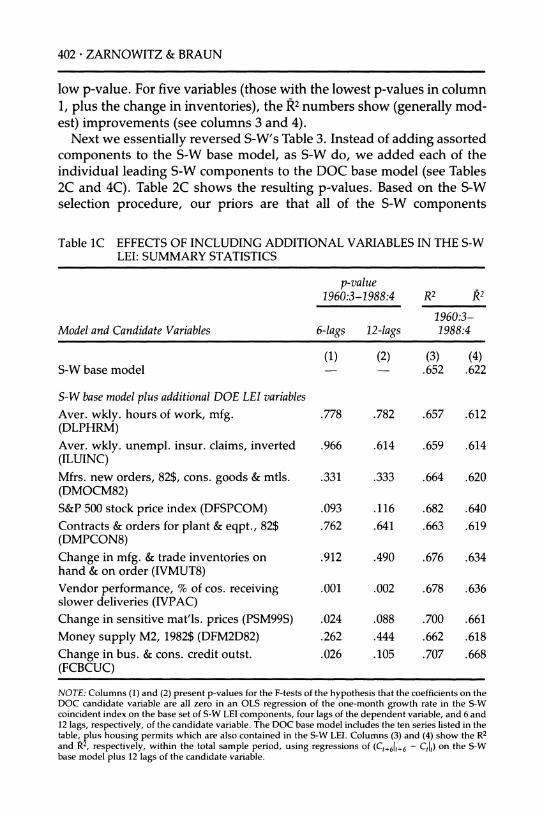
402 * ZARNOWITZ & BRAUN
low p-value. For five variables (those with the lowest p-values in column 1, plus the change in inventories), the R2 numbers show (generally mod- est) improvements (see columns 3 and 4).
Next we essentially reversed S-W's Table 3. Instead of adding assorted
components to the S-W base model, as S-W do, we added each of the individual leading S-W components to the DOC base model (see Tables 2C and 4C). Table 2C shows the resulting p-values. Based on the S-W selection procedure, our priors are that all of the S-W components
Table 1C EFFECTS OF INCLUDING ADDITIONAL VARIABLES IN THE S-W LEI: SUMMARY STATISTICS
p-value 1960:3-1988:4 R2 R2
1960:3- Model and Candidate Variables 6-lags 12-lags 1988:4
(1) (2) (3) (4) - .652 .622 S-W base model
S-W base model plus additional DOE LEI variables
Aver. wkly. hours of work, mfg. (DLPHRM) Aver. wkly. unempl. insur. claims, inverted (ILUINC) Mfrs. new orders, 82$, cons. goods & mtls. (DMOCM82) S&P 500 stock price index (DFSPCOM) Contracts & orders for plant & eqpt., 82$ (DMPCON8) Change in mfg. & trade inventories on hand & on order (IVMUT8) Vendor performance, % of cos. receiving slower deliveries (IVPAC) Change in sensitive mat'ls. prices (PSM99S) Money supply M2, 1982$ (DFM2D82) Change in bus. & cons. credit outst. (FCBCUC)
.778 .782 .657 .612
.966 .614 .659 .614
.331 .333 .664 .620
.093 .116 .682 .640
.762 .641 .663 .619
.912 .490 .676 .634
.001 .002 .678 .636
.024
.262
.026
.088 .700 .661
.444 .662 .618
.105 .707 .668
NOTE: Columns (1) and (2) present p-values for the F-tests of the hypothesis that the coefficients on the DOC candidate variable are all zero in an OLS regression of the one-month growth rate in the S-W coincident index on the base set of S-W LEI components, four lags of the dependent variable, and 6 and 12 lags, respectively, of the candidate variable. The DOC base model includes the ten series listed in the table, plus housing permits which are also contained in the S-W LEI. Columns (3) and (4) show the R2 and R2, respectively, within the total sample period, using regressions of (Ct+61t+6 - Ctlt) on the S-W base model plus 12 lags of the candidate variable.
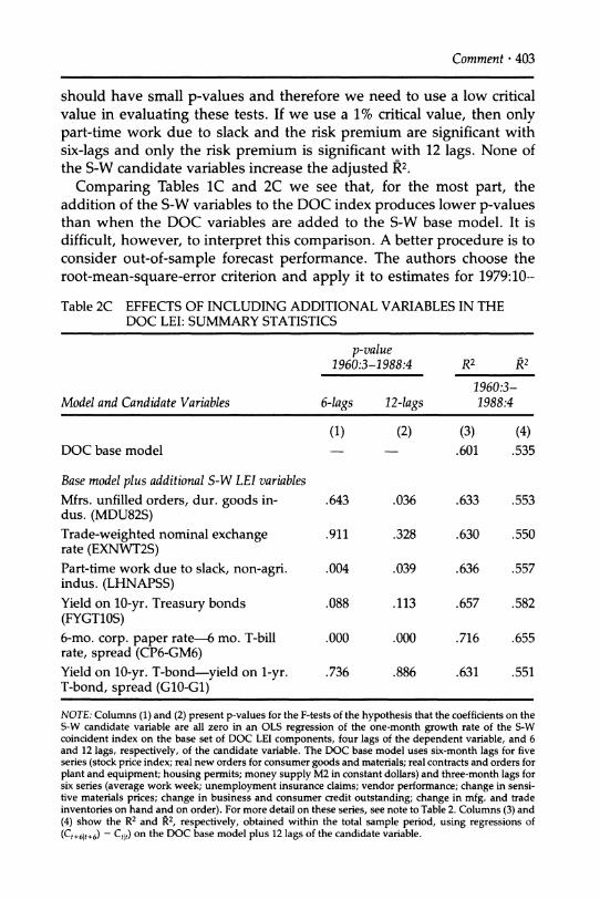
Comment 403
should have small p-values and therefore we need to use a low critical value in evaluating these tests. If we use a 1% critical value, then only part-time work due to slack and the risk premium are significant with
six-lags and only the risk premium is significant with 12 lags. None of the S-W candidate variables increase the adjusted R2.
Comparing Tables 1C and 2C we see that, for the most part, the addition of the S-W variables to the DOC index produces lower p-values than when the DOC variables are added to the S-W base model. It is difficult, however, to interpret this comparison. A better procedure is to consider out-of-sample forecast performance. The authors choose the
root-mean-square-error criterion and apply it to estimates for 1979:10-
Table 2C EFFECTS OF INCLUDING ADDITIONAL VARIABLES IN THE DOC LEI: SUMMARY STATISTICS
p-value 1960:3-1988:4 R2 R2
1960:3- Model and Candidate Variables 6-lags 12-lags 1988:4
(1) (2) (3) (4) DOC base model .601 .535
Base model plus additional S-W LEI variables Mfrs. unfilled orders, dur. goods in- .643 .036 .633 .553 dus. (MDU82S) Trade-weighted nominal exchange .911 .328 .630 .550 rate (EXNWT2S) Part-time work due to slack, non-agri. .004 .039 .636 .557 indus. (LHNAPSS) Yield on 10-yr. Treasury bonds .088 .113 .657 .582 (FYGT10S) 6-mo. corp. paper rate-6 mo. T-bill .000 .000 .716 .655 rate, spread (CP6-GM6) Yield on 10-yr. T-bond-yield on 1-yr. .736 .886 .631 .551 T-bond, spread (G10-G1)
NOTE: Columns (1) and (2) present p-values for the F-tests of the hypothesis that the coefficients on the S-W candidate variable are all zero in an OLS regression of the one-month growth rate of the S-W coincident index on the base set of DOC LEI components, four lags of the dependent variable, and 6 and 12 lags, respectively, of the candidate variable. The DOC base model uses six-month lags for five series (stock price index; real new orders for consumer goods and materials; real contracts and orders for plant and equipment; housing permits; money supply M2 in constant dollars) and three-month lags for six series (average work week; unemployment insurance claims; vendor performance; change in sensi- tive materials prices; change in business and consumer credit outstanding; change in mfg. and trade inventories on hand and on order). For more detail on these series, see note to Table 2. Columns (3) and (4) show the R2 and R2, respectively, obtained within the total sample period, using regressions of (Ct+61t+6) - Ctt) on the DOC base model plus 12 lags of the candidate variable.
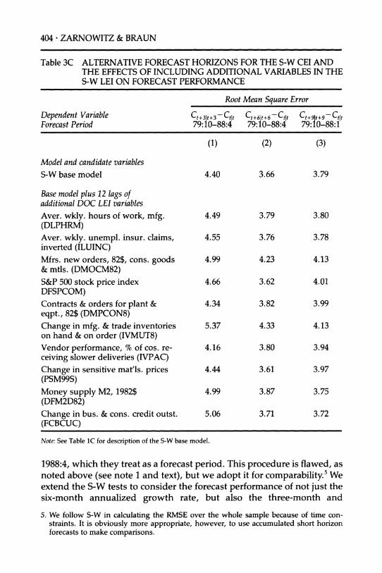
404 * ZARNOWITZ & BRAUN
Table 3C ALTERNATIVE FORECAST HORIZONS FOR THE S-W CEI AND THE EFFECTS OF INCLUDING ADDITIONAL VARIABLES IN THE S-W LEI ON FORECAST PERFORMANCE
Root Mean Square Error
Dependent Variable Ct+31t+3-Ctlt Ct+6+6 -Ctt Ct+9t+9-Ctlt Forecast Period 79:10-88:4 79:10-88:4 79:10-88:1
(1) (2) (3)
Model and candidate variables S-W base model 4.40 3.66 3.79
Base model plus 12 lags of additional DOC LEI variables Aver. wkly. hours of work, mfg. 4.49 3.79 3.80 (DLPHRM) Aver. wkly. unempl. insur. claims, 4.55 3.76 3.78 inverted (ILUINC) Mfrs. new orders, 82$, cons. goods 4.99 4.23 4.13 & mtls. (DMOCM82) S&P 500 stock price index 4.66 3.62 4.01 DFSPCOM) Contracts & orders for plant & 4.34 3.82 3.99 eqpt., 82$ (DMPCON8) Change in mfg. & trade inventories 5.37 4.33 4.13 on hand & on order (IVMUT8) Vendor performance, % of cos. re- 4.16 3.80 3.94 ceiving slower deliveries (IVPAC) Change in sensitive mat'ls. prices 4.44 3.61 3.97 (PSM99S) Money supply M2, 1982$ 4.99 3.87 3.75 (DFM2D82) Change in bus. & cons. credit outst. 5.06 3.71 3.72 (FCBCUC)
Note: See Table 1C for description of the S-W base model.
1988:4, which they treat as a forecast period. This procedure is flawed, as noted above (see note 1 and text), but we adopt it for comparability.5 We extend the S-W tests to consider the forecast performance of not just the six-month annualized growth rate, but also the three-month and
5. We follow S-W in calculating the RMSE over the whole sample because of time con- straints. It is obviously more appropriate, however, to use accumulated short horizon forecasts to make comparisons.
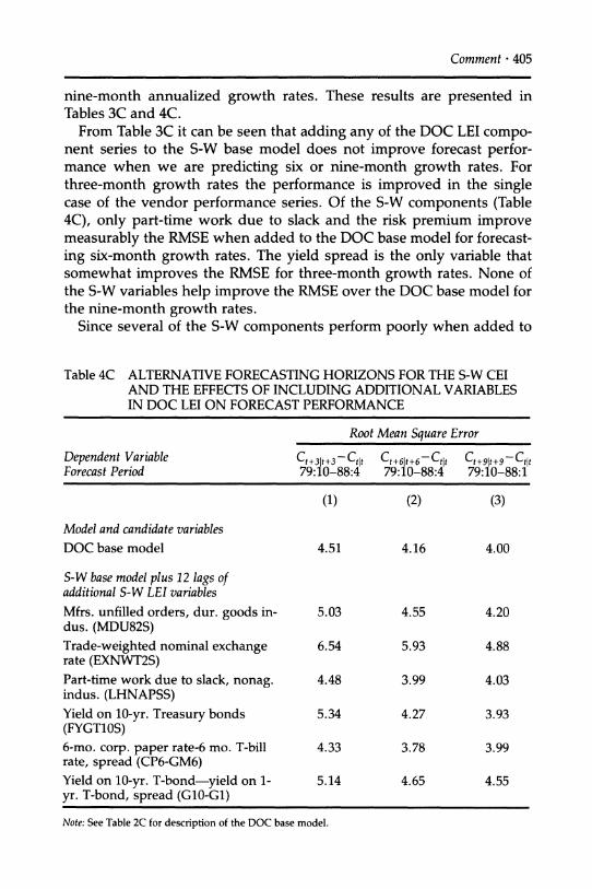
Comment * 405
nine-month annualized growth rates. These results are presented in Tables 3C and 4C.
From Table 3C it can be seen that adding any of the DOC LEI compo- nent series to the S-W base model does not improve forecast perfor- mance when we are predicting six or nine-month growth rates. For three-month growth rates the performance is improved in the single case of the vendor performance series. Of the S-W components (Table 4C), only part-time work due to slack and the risk premium improve measurably the RMSE when added to the DOC base model for forecast-
ing six-month growth rates. The yield spread is the only variable that somewhat improves the RMSE for three-month growth rates. None of the S-W variables help improve the RMSE over the DOC base model for the nine-month growth rates.
Since several of the S-W components perform poorly when added to
Table 4C ALTERNATIVE FORECASTING HORIZONS FOR THE S-W CEI AND THE EFFECTS OF INCLUDING ADDITIONAL VARIABLES IN DOC LEI ON FORECAST PERFORMANCE
Root Mean Square Error
Dependent Variable Ct+3t+3 -C tt Ct+6t+6 -Ctlt Forecast Period 79:10-88:4 79:10-88:4 79:10-88:1
(1) (2) (3)
Model and candidate variables DOC base model 4.51 4.16 4.00
S-W base model plus 12 lags of additional S-W LEI variables Mfrs. unfilled orders, dur. goods in- 5.03 4.55 4.20 dus. (MDU82S) Trade-weighted nominal exchange 6.54 5.93 4.88 rate (EXNWT2S) Part-time work due to slack, nonag. 4.48 3.99 4.03 indus. (LHNAPSS) Yield on 10-yr. Treasury bonds 5.34 4.27 3.93 (FYGT10S) 6-mo. corp. paper rate-6 mo. T-bill 4.33 3.78 3.99 rate, spread (CP6-GM6) Yield on 10-yr. T-bond-yield on 1- 5.14 4.65 4.55 yr. T-bond, spread (G10-G1)
Note: See Table 2C for description of the DOC base model.
406 ZARNOWITZ & BRAUN
the DOC base set, one would wish to exclude them when trying to
improve the DOC LEI. This is analogous to what S-W conclude with reference to the inclusion of candidate DOC base variables in their LEI. However, the comparison of the R2 and RMSE statistics for the alterna- tive base models suggests that, taken as a whole, the S-W LEI performs better than the DOC LEI over the periods considered.
The same conclusion emerges from an attempt to compare how well the two LEIs perform in forecasting real GNP growth. We produced one-
step ahead forecasts of real GNP from a naive AR(3) model, updating the
parameter estimates every period, and calculated the RMSE over the
period 1979:3 through 1988:1. The RMSE for the naive model was .00997. When we added three lags of the S-W LEI, the RMSE fell to .00863. When we alternatively added three lags of growth rates of the DOC LEI to the naive model, the RMSE only fell to .00935. These results again indicate that the S-W base model taken as a set performs well compared to the DOC LEI.
When the sample period is extended back, from 1960-79 to 1948-79, the RMSE for real growth 1979-88 forecasts from the AR(3) model de- clines 1.2% to .00985, while the RMSE for the corresponding forecasts with DOC LEI declines 8.0% to .00917. (For lack of data, we could not make a similar calculation for forecasts with S-W LEI.)
Concluding Remarks Our review of the S-W work and additional tests suggest the following points: 1. The proposed LEI performs relatively well in forecasting the rate of
growth in real economic activity (represented either by CEI or GNP) over the periods considered in this study. To some extent, this result reflects the search and other procedures adopted by S-W, and hence, it could well apply mainly to these periods. The S-W LEI is better as a set than are its individual components, but the same can be said of the DOC LEI. 2. Comparisons of the two LEI's are difficult because their objectives and construction are substantively different. When the S-W goal, rates, and time frame are adopted, the S-W LEI gives better results, which may not be surprising and is certainly not conclusive. The DOC LEI has a more
comprehensive coverage based on a much longer historical experience. This could well prove an advantage over time inasmuch as the causes of business cycles may vary. On the other hand, the DOC LEI may suffer more from overfitting or redundancies over limited time periods. 3. To assess the predictive performance of the S-W LEI, out-of-sample measures are needed, which are now lacking because the index is con-
Comment 407
structed from data for the entire period covered. The sample and fore- cast periods must be distinguished, and a sensitivity analysis using dif- ferent breakdowns of the available data would be desirable. There are indications that the DOC LEI predicts better in a model based on a
longer sample period. In any event, it would be well to extend the S-W LEI back ten years as well, to cover the recessions of 1948-49, 1953-54, and 1957-58. 4. Some components of the S-W LEI contribute much, others little when added to the DOC LEI: compare, e.g., the strongly favorable evidence for the risk premium (CP6-GM6) with the poor one for the yield spread (G10- G1). The inclusion of the nominal exchange rate is particularly question- able. Similarly, there are also large differences in performance between the components of DOC-LEI. It is possible that a combination of the best series from both sets would result in significant improvements. This may form a part of a promising research agenda for further study. 5. More components are smoothed in the S-W LEI than in the DOC LEI, which may favor the former. Also, the incorporation of the most recent information available for some of the S-W index components should be on the average rewarding, and the same probably applies to the determi- nation of the lag structures in this index. It would be possible to take
advantage of some of these innovations in the DOC LEI as well. 6. S-W have a specific target and focus on six-month growth in their CEI, whereas the DOC LEI has been more flexibly designed and used. This is a basic difference, which has important implications that deserve to be studied. 7. Because of time limitations, we have not been able to examine the S-W Recession Index, an ambitious project growing out of the important work by Wecker and Diebold and Rudebusch. But it may be worth
noting that we would expect the Recession Index to share many of the
strengths and weaknesses of S-W LEI because of large elements of com- mon coverage.
REFERENCES
Auerbach, A. J. 1982. "The Index of Leading Indicators: 'Measurement Without Theory,' Thirty-five Years Later." Review of Economics and Statistics 64: No. 4 589-95.
Burns, A. F and W. C. Mitchell. 1946. Measuring Business Cycles. New York: NBER.
Diebold, F X. and G. D. Rudebusch. 1987. "Scoring the Leading Indicators." Federal Reserve Board, Division of Research and Statistics. Manuscript.
Haberler, Gottfried. Prosperity and Depression. New edition. First published by the League of Nations. Cambridge, Mass.: Harvard University Press. [1937] 1964.
408 * DISCUSSION
Koch, P. D. and R. H. Raasche. 1988. "An Examination of the Commerce Depart- ment Leading-Indicator Approach." Journal of Business and Economic Statistics 6: No. 2 167-87.
Moore, G. H. 1983. Business Cycles, Inflation, and Forecasting, 2nd edition, Cam- bridge, Mass.: Ballinger Publishing Company for NBER.
Neftci, S. N. 1982. "Optimal Prediction of Cyclical Downturns." Journal of Eco- nomic Dynamics and Control 4: 225-41.
Vaccara, B. N., and V. Zarnowitz. 1978. "Forecasting with the Index of Leading Economic Indicators." NBER Working Paper No. 244.
Zarnowitz, V. "Recent Work on Business Cycles in Historical Perspective: A Review of Theories and Evidence." Journal of Economic Literature, Vol. 23(2). pp. 523-80. June 1985.
Zarnowitz, V. and P. Braun. "Major Macroeconomic Variables and Leading In- dexes: Some Estimates of Their Interrelations, 1886-1982." NBER Working Paper No. 2812. January 1989.
Zarnovitz, V. and G. H. Moore. 1982. "Sequential Signals of Recession and Recovery." Journal of Business 55: No. 1 57-85.
Discussion
Watson stressed that the model appeared stable over different samples and that since the equation was only approximate, the six month fore- cast is appropriate.
Bob Hall stated that this work is NBER-supported but is not an official NBER publication. He also asked what predictive value should be as-
signed to the different variables in the LEI. Watson replied that the
corporate paper/T-bill spread is important but not completely dominant; interest rates and exchange rates are less important. Hall asked what the model currently forecasts. Watson responded that the coincident index is projected to increase 2.6% in the next six months and the probability of a recession in that period is .05; the probability of a recession in the next year is .27.
Ben Friedman noted that monetary policy affects output only if the T- bill rate is used, not the commercial paper rate, as observed by Sims in his monetary policy study. In recent periods, there is no liquidity differ- ence between the two bills, but there is a default premium in the private debt. This is a good economic indicator since defaults tend to occur when the economy is in decline. As a result, the relationship above is rational and furthermore, it is not surprising to find it currently rather than in previous data.
Sims responded that it is unclear why defaults should be cyclical, but Friedman stated that regardless of the real effects of defaults, their cycli- cality is well-established.


![Using High Frequency Indicators in Trinidad and Tobago ... · leading, lagging and coincident ... Microsoft PowerPoint - Using High Frequency Indicators in Trinidad and Tobago [Read-Only]](https://img.pdfslide.net/doc/110x75/5b795bce7f8b9a534c8d26df/using-high-frequency-indicators-in-trinidad-and-tobago-leading-lagging.jpg)