HAL Id: hal-02324233https://hal.archives-ouvertes.fr/hal-02324233

Submitted on 15 Jun 2020

HAL is a multi-disciplinary open accessarchive for the deposit and dissemination of sci-entific research documents, whether they are pub-lished or not. The documents may come fromteaching and research institutions in France orabroad, or from public or private research centers.

L’archive ouverte pluridisciplinaire HAL, estdestinée au dépôt et à la diffusion de documentsscientifiques de niveau recherche, publiés ou non,émanant des établissements d’enseignement et derecherche français ou étrangers, des laboratoirespublics ou privés.

New insights into the reproductive cycle of two GreatScallop populations in Brittany (France) using a DEB

modelling approachMélaine Gourault, Romain Lavaud, Aude Leynaert, Laure Pecquerie,

Yves-Marie Paulet, Stéphane Pouvreau

To cite this version:Mélaine Gourault, Romain Lavaud, Aude Leynaert, Laure Pecquerie, Yves-Marie Paulet, et al..New insights into the reproductive cycle of two Great Scallop populations in Brittany (France) us-ing a DEB modelling approach. Journal of Sea Research (JSR), Elsevier, 2019, 143, pp.207-221.�10.1016/j.seares.2018.09.020�. �hal-02324233�

1

Please note that this is an author-produced PDF of an article accepted for publication following peer review. The definitive publisher-authenticated version is available on the publisher Web site.

Journal of Sea Research January 2019, Volume 143, Pages 207-221 http://dx.doi.org/10.1016/j.seares.2018.09.020 http://archimer.ifremer.fr/doc/00458/57012/

Archimer http://archimer.ifremer.fr

New insights into the reproductive cycle of two Great Scallop populations in Brittany (France) using a DEB

modelling approach

Gourault Mélaine 4, *

, Lavaud Romain 2, Leynaert Aude

3, Pecquerie Laure

3, Paulet Yves-Marie

3,

Pouvreau Stéphane 1

1 Ifremer, Laboratoire des Sciences de l'Environnement Marin (LEMAR), 29840 Argenton-en-

Landunvez, France 2 Fisheries and Oceans Canada, Moncton, NB E1C 9B6, Canada

3 Laboratoire des Sciences de l'Environnement Marin (LEMAR), UBO, CNRS, IRD, Ifremer, Plouzané,

France

* Corresponding author : Mélaine Gourault, email address : melaine.gourault@gmail.com

Abstract : The present study aimed to improve understanding of the environmental conditions influencing the reproductive cycle of the great scallop Pecten maximus in two locations in Brittany (France). We also evaluated potential consequences of future climate change for reproductive success in each site.

We simulated reproductive traits (spawning occurrences and synchronicity among individuals) of P. maximus, using an existing Dynamic Energy Budget (DEB) model. To validate and test the model, we used biological and environmental datasets available for the Bay of Brest (West Brittany, France) between 1998 and 2003. We also applied the scallop DEB model in the Bay of Saint-Brieuc (North Brittany, France) for the same period (1998–2003) to compare the reproductive cycle in different environmental conditions. In order to accurately model the P. maximus reproductive cycle we improved the scallop DEB model in two ways: through (1) energy acquisition, by incorporating microphytobenthos as a new food source; and (2) the reproductive process, by adding a new state variable dedicated to the gamete production. Finally, we explored the effects of two contrasting IPCC climate scenarios (RCP2.6 and RCP8.5) on the reproductive cycle of P. maximus in these two areas at the 2100 horizon.

In the Bay of Brest, the simulated reproductive cycle was in agreement with field observations. The model reproduced three main spawning events every year (between May and September) and asynchronicity in the timing of spawning between individuals. In the Bay of Saint-Brieuc, only two summer spawning events (in July and August) were simulated, with a higher synchronicity between individuals. Environmental conditions (temperature and food sources) were sufficient to explain this well-known geographic difference in the reproductive strategy of P. maximus. Regarding the forecasting approach, the model showed that, under a warm scenario (RCP8.5), autumnal spawning would be enhanced at the 2100 horizon with an increase of seawater temperature in the Bay of Brest, whatever the food source conditions. In the Bay of Saint-Brieuc, warmer temperatures may impact reproductive

2

Please note that this is an author-produced PDF of an article accepted for publication following peer review. The definitive publisher-authenticated version is available on the publisher Web site.

phenology through an earlier onset of spawning by 20 to 44 days depending on the year.

Highlights

► We aimed at better understanding and quantifying the effect of environmental variables (temperature and food sources) on the reproduction variability of the Great Scallop Pecten maximus in Brittany. ► We improved an existing scallop-DEB model at two different levels, by adding a new food source and a more detailed reproduction module. ► We compared reproductive traits of the Great Scallop in two Brittany locations for the period 1998–2003 and we made forecasts at the 2100 horizon within a context of ocean warming. ► We evidenced two different effects of the increase of seawater temperature depending on the location: a most efficient autumnal last spawning in the Bay of Brest and an earlier onset of spawning in the Bay of Saint-Brieuc.

Keywords : Pecten maximus, DEB theory, reproduction cycle, IPCC scenarios, Bay of Brest, Bay of Saint-Brieuc

ACC

EPTE

D M

ANU

SCR

IPT

4

1. Introduction 47

The great scallop, Pecten maximus (Linnaeus, 1758) inhabits many sublittoral environments 48

along Northeast Atlantic coasts from northern Norway to the Iberian Peninsula (Ansell et al., 1991). In 49

France, the species is particularly abundant along the coast of northern Brittany, where it sustains one 50

of the most important French commercial fisheries both in terms of landings and of socio-economic 51

value (more than 300 fishing boats; ICES, 2015). The main fishing areas are located in the Bay of 52

Brest, connected to the Iroise Sea, and in the Bay of Saint-Brieuc, open to the English Channel (Fig. 53

1). While some of the highest scallop densities are found in the Bay of Saint-Brieuc, in part due to 54

sustainable exploitation measures, the scallop stock in the Bay of Brest is lower and highly dependent 55

on hatchery produced spat since 1983. 56

From a biological point of view, scallops, like most other bivalves, are filter feeders and 57

consume phytoplankton. However, since they live settled into the surface layer of the bottom, they are 58

also thought to use the epibenthic layer as an important food source (see review in Shumway, 1990). 59

Concerning the reproductive cycle, P. maximus is a functional hermaphrodite species, it has a pelagic 60

larval stage during approximately one month after fertilization, switching to a benthic life after 61

metamorphosis. Its reproductive strategy is more surprising as its spawning period varies according to 62

the geographical location of the population (see review by Gosling (2004)) There can be between one 63

major summer spawning and more than three spawnings in the period from spring to early autumn. At 64

a small regional scale, geographical differences can be very marked: scallops from the Bay of Brest 65

show low inter-individual synchronism, with multiple partial spawnings from early spring to autumn 66

and almost no resting stage, whereas the population from the Bay of St-Brieuc is almost synchronous, 67

with one or two major spawnings over a short period (July-August), with a sexual rest stage then 68

observed in autumn and winter (e.g. Devauchelle and Mingant, 1991; Paulet et al., 1997). 69

A major part of this phenotypic variability has been attributed to differences in environmental 70

conditions such as food sources, temperature and photoperiod, which are known to influence 71

gametogenesis and fecundity in marine invertebrates. For example, Claereboudt and Himmelman 72

(1996) showed that an increase in temperature and food availability increased reproductive effort in 73

ACCEPTED MANUSCRIPT

ACC

EPTE

D M

ANU

SCR

IPT

5

Placopecten magellanicus. In P. maximus, quantity and quality of food sources also have an impact on 74

hatching rate (Soudant et al., 1996), and laboratory experiments showed that spring conditions (regular 75

increase of temperature and photoperiod) favoured gonad growth, whereas winter conditions (regular 76

decrease of temperature and daylight duration) were associated with somatic growth of the adductor 77

muscle and digestive gland (Saout et al., 1999; Lorrain et al., 2002). More recently, Chauvaud et al., 78

(2012) and Lavaud et al. (2014) have proposed complementary approaches to quantitatively evaluate 79

effects on environmental factors on growth and reproduction of scallops. However, the relative 80

importance of these variables remains difficult to disentangle, especially under natural conditions. 81

Climate models and observations to date indicate that the Earth will warm between two (IPCC 82

scenario RCP2.6) and six degrees Celsius (IPCC scenario RCP8.5) over the next century, depending 83

on how fast carbon dioxide emissions increase. The ocean absorbs most of this excess heat, leading to 84

rising seawater temperatures (e.g., IPCC, 2014; Appendix A). Increasing ocean temperatures will 85

deeply affect marine species and ecosystems. Understanding the potential effects of climate change on 86

the timing of life-history events such as the onset of gametogenesis, spawning, hatching and larval 87

metamorphosis is important for benthic ecology but also for aquaculture and fisheries production. The 88

phenology of these key life-history events has been investigated in several ecosystems and in many 89

species (e.g., Beukema et al., 2009; Menge et al., 2009; Shephard et al., 2010; Valdizan et al., 2011; 90

Morgan et al., 2013), although these studies often had limited spatial and/or temporal resolution. 91

Mechanistic modelling provides a complementary tool to analyse climate effects on life-history traits, 92

identify interactions between multiple stressors, and make predictions about future condition scenarios 93

at a larger spatiotemporal scale. In recent decades, bivalve growth and reproduction have been 94

successfully modelled (e.g. Bernard et al., 2011; Thomas et al., 2016; Montalto et al., 2017; Gourault 95

et al., 2018, this issue) using mechanistic models based on Dynamic Energy Budget theory (DEB; 96

Kooijman, 2010). This theory makes it possible to quantify the energy flows within an individual from 97

ingestion to maintenance, growth, development, and reproduction in relation to environmental 98

conditions. 99

ACCEPTED MANUSCRIPT

ACC

EPTE

D M

ANU

SCR

IPT

6

In this context, the present study aims to improve understanding of the environmental factors 100

influencing the reproductive cycle of P. maximus using a DEB model and the potential effects of 101

climate change on the reproductive activity of this species. Our work is based on an existing DEB 102

model developed for the great scallop in the Bay of Brest (Lavaud et al. 2014) that we then improved 103

by adding detail on the reproductive processes. To evaluate the ability of the model to simulate 104

reproductive processes under various conditions, we tested it over six years in the Bay of Brest (1998–105

2003) and in the two main locations hosting scallop populations in Brittany: the Bay of Brest and the 106

Bay of Saint-Brieuc. In a second step, using two IPCC climate scenarios at the 2100 horizon, we 107

examined the potential consequences of future climate change on the reproductive activity of this 108

emblematic species in each of the two sites. 109

ACCEPTED MANUSCRIPT

ACC

EPTE

D M

ANU

SCR

IPT

7

2. Material and Methods 110

2.1. Study sites 111

The Bay of Brest is a semi-enclosed coastal ecosystem located in western Brittany, France, 112

connected to the Atlantic Ocean by a deep narrow strait. The bay itself covers an area of nearly 180 113

km², with an average depth of 8 m. Two rivers flow into the bay: the Elorn (watershed of 402 km²) and 114

the Aulne (watershed of 1842 km²) (Fig. 1). Temperature and phytoplankton concentration are 115

continuously monitored at two locations in the Bay: Lanvéoc station in the southern part of the Bay 116

(data provided by the REPHY network - Phytoplankton and Phycotoxin monitoring NEtwork, Ifremer, 117

e.g. Belin et al., 2017) and Sainte-Anne station in the north-western part (data provided by the 118

SOMLIT - “Service d'Observation en Milieu Littoral”, INSU-CNRS, Brest). Lanvéoc station (48°29’ 119

N, 04°46’ W; Fig. 1) has a depth range of 6 to 9 m at lowest spring tides and a bottom composed of 120

sandy mud, with broken shells and pebbles. Sainte-Anne station is located at the entrance to the Bay of 121

Brest (48°21’’ N, 04°33 W; Fig. 1). 122

The Bay of Saint-Brieuc is located in northern Brittany (France), 150 km from the Bay of Brest 123

(48°32N, 02°40W; Fig. 1), in the western part of the English Channel. This bay of 800 km2 harbours a 124

large wild scallop population in its inshore shallow waters (≤ 30 m). It is subject to an extreme tidal 125

regime with a tidal range between 4 m at neap tides and nearly 13 m during spring tides. Seawater 126

temperature and phytoplankton concentration are monitored at the Bréhat station located in the 127

western part of the bay (Fig. 1). 128

ACCEPTED MANUSCRIPT

ACC

EPTE

D M

ANU

SCR

IPT

8

129

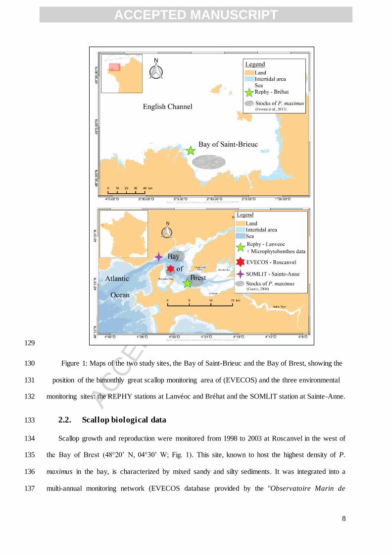
Figure 1: Maps of the two study sites, the Bay of Saint-Brieuc and the Bay of Brest, showing the 130

position of the bimonthly great scallop monitoring area of (EVECOS) and the three environmental 131

monitoring sites: the REPHY stations at Lanvéoc and Bréhat and the SOMLIT station at Sainte-Anne. 132

2.2. Scallop biological data 133

Scallop growth and reproduction were monitored from 1998 to 2003 at Roscanvel in the west of 134

the Bay of Brest (48°20’ N, 04°30’ W; Fig. 1). This site, known to host the highest density of P. 135

maximus in the bay, is characterized by mixed sandy and silty sediments. It was integrated into a 136

multi-annual monitoring network (EVECOS database provided by the "Observatoire Marin de 137

ACCEPTED MANUSCRIPT

ACC

EPTE

D M

ANU

SCR

IPT

9

l’IUEM, Brest, France"). A sample of 20 adult scallops (3 years old) was collected by dredging on a 138

biweekly to monthly basis in 30-m deep waters. The scallops were brought back to the laboratory 139

where the muscle, gonads and digestive gland were dissected out. Total wet flesh mass and total dry 140

flesh mass (DFM) of each organ were measured for each individual. In order to compare masses 141

obtained for different sized scallops, dry mass was standardized following the formula of Bayne et al. 142

(1987): 143

(

)

144

where is the standardized mass of an individual of standard shell height and is the measured 145

mass of an individual of measured shell height . Length and mean daily shell growth rate (DSGR) 146

were measured according to the method proposed by Chauvaud et al. (2012) (see Lavaud et al. 2014 147

for more detailed information on these data). 148

Additionally, four additional P. maximus reproductive cycle traits were recorded through 149

EVECOS monitoring: the onset of gametogenesis, the number and timing of each main spawning 150

within the reproductive season and the reproductive investment (DFM difference before and after 151

spawning). 152

2.3. The scallop DEB model 153

The scallop DEB model was derived from the standard DEB model described by Kooijman 154

(2010) and first applied to P. maximus by Lavaud et al. (2014). The DEB model is a mechanistic 155

model that describes the dynamics of three state variables: E, the energy in reserve, V, the volume of 156

structure, and ER, the energy allocated to development and reproduction. To improve the accuracy 157

with which DEB models model reproductive activity, Bernard et al. (2011) refined the processes of 158

energy allocation to gametogenesis and resorption in the model, such that a fourth state variable, EGO, 159

the energy in gametes, was added to the existing scallop DEB model (Fig. 2). Briefly, the model can 160

be explained as follows: the reserve mobilization rate, ̇ , is divided into two parts. A first constant 161

fraction, ??, is allocated to structural growth and maintenance and the remainder, 1-??, is allocated to 162

development (in juveniles), reproduction (in adults) and maturity maintenance. Energy allocation to 163

ACCEPTED MANUSCRIPT

ACC

EPTE

D M

ANU

SCR

IPT

10

gonad construction is modelled through the gamete mobilization rate, ̇ . Priority in energy allocation 164

is always given to maintenance costs: ̇ for maturity maintenance and ̇ for somatic maintenance. 165

During starvation periods, the gametogenesis flux is re-allocated to somatic and maturity maintenance 166

through secondary maintenance, ̇ . If ̇ does not provide enough energy to cover all maintenance 167

costs, the gamete resorption rate, ̇ , is activated. In case of extreme starvation, structure can be 168

broken down at the rate ̇ . The corresponding set of equations can be found in Gourault et al. (2018, 169

this issue). 170

Regarding food assimilation, a classical scaled functional response (Holling type II) is 171

generally calculated in the model (Kooijman, 2010), using one food source (for bivalves, this 172

essentially consists of phytoplankton cells). However, many studies focusing on modelling the energy 173

dynamics of filter feeders have shown the need and benefit of adding a second food source to improve 174

the food proxy (Alunno-Bruscia et al, 2011; Bernard et al., 2011; Saraiva et al., 2011). Lavaud et al. 175

(2014) included the Synthesizing Units (SUs) concept (Kooijman, 2010; Saraiva et al. 2011) into the 176

scallop DEB model to consider selection of particles based on their size and/or quality. The equations 177

for the SU concept can be found in Lavaud et al. (2014). 178

In this study we compared the previous model of Lavaud et al. (2014), hereafter referred to as 179

“Mod-1”, with our DEB model (with the extra state variable EGO), hereafter referred to as “Mod-2” 180

(Table 1). Two versions of the Mod-2 model were used in order to test different food sources in the 181

model: (1) phytoplankton as a first food proxy and particulate organic matter (POM) as a second food 182

proxy (Mod-2A) and (2) a mix of microphytobenthos and phytoplankton as a first food proxy and 183

POM as a second food proxy (Mod-2B). All the model parameters are given in Table 2. Simulations 184

were performed using R software (3.3.3 version). 185

186

ACCEPTED MANUSCRIPT

ACC

EPTE

D M

ANU

SCR

IPT

11

187

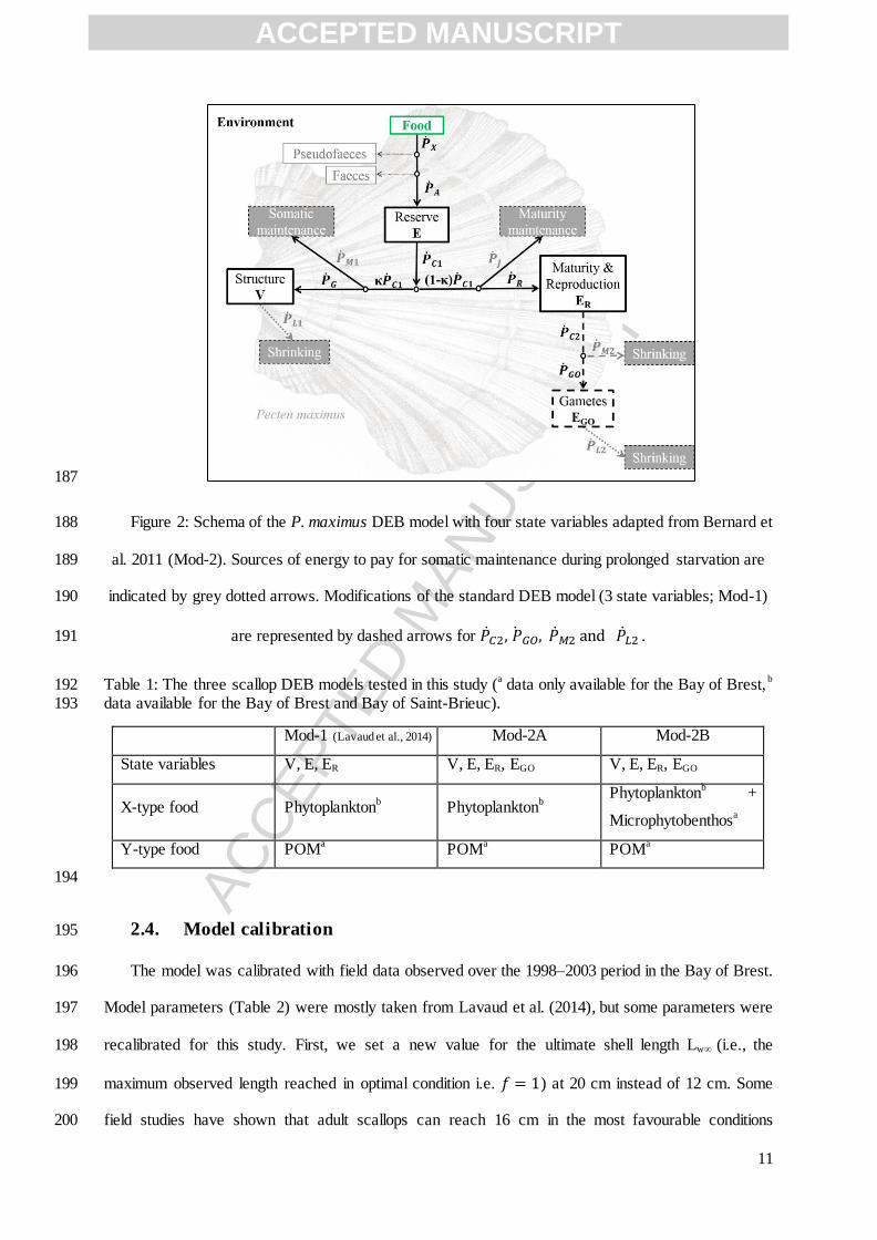
Figure 2: Schema of the P. maximus DEB model with four state variables adapted from Bernard et 188

al. 2011 (Mod-2). Sources of energy to pay for somatic maintenance during prolonged starvation are 189

indicated by grey dotted arrows. Modifications of the standard DEB model (3 state variables; Mod-1) 190

are represented by dashed arrows for ̇ ̇ ̇ ̇ . 191

Table 1: The three scallop DEB models tested in this study (a data only available for the Bay of Brest,

b 192

data available for the Bay of Brest and Bay of Saint-Brieuc). 193

Mod-1 (Lavaud et al., 2014) Mod-2A Mod-2B

State variables V, E, ER V, E, ER, EGO V, E, ER, EGO

X-type food Phytoplanktonb Phytoplankton

b

Phytoplanktonb +

Microphytobenthosa

Y-type food POMa POM

a POM

a

194

2.4. Model calibration 195

The model was calibrated with field data observed over the 1998–2003 period in the Bay of Brest. 196

Model parameters (Table 2) were mostly taken from Lavaud et al. (2014), but some parameters were 197

recalibrated for this study. First, we set a new value for the ultimate shell length Lw∞ (i.e., the 198

maximum observed length reached in optimal condition i.e. ) at 20 cm instead of 12 cm. Some 199

field studies have shown that adult scallops can reach 16 cm in the most favourable conditions 200

ACCEPTED MANUSCRIPT

ACC

EPTE

D M

ANU

SCR

IPT

12

(Mason, 1957; Chauvaud et al., 2012), so we set L∞ above this value. According to DEB theory, is 201

calculated through the following equation: 202

( { ̇ }[ ̇ ]

)

where { ̇ } is the maximum surface specific assimilation, [ ̇ ] is the volume-specific maintenance 203

costs, is the allocation fraction to growth and maintenance and is the shape coefficient. We 204

modified the values of κ, { ̇Am} and [ ̇M], while keeping . We estimated the values of { ̇Am} 205

from Strohmeier et al. (2009) and a known value of [ ̇M] at the same reference temperature (Emmery, 206

2008). Therefore, we were able to recalculate . 207

To account for variability in the initial conditions between individuals, we simulated 20 208

individuals in each scenario (i.e., 20 different individual growth trajectories) by setting 20 different 209

initial conditions of size and weight (i.e., first sampling of the year from EVECOS monitoring). Initial 210

values for the four state variables (E, V, ER and EGO) were calculated using the equations given in 211

Table 3 from the measurements obtained in the first sampling of the year. Individual growth 212

simulations were then pooled together to compute average growth patterns and standard deviation. 213

Three parameters control spawning in our model: the gonado-somatic ratio GSI, photoperiod and 214

phytoplankton concentration. Threshold values for each of these three parameters were set as follows: 215

GSI = 15% (estimated according to biological data from EVECOS monitoring), photoperiod (Photo) = 216

14 hours (spawning is possible only if the daylength is above 14 h; Saout et al., 1999) and a 217

phytoplankton concentration threshold (Phyto) = 2.50 105 cell L

-1 (average value corresponding to the 218

beginning of a spring bloom; Paulet et al., 1997). In contrast to Lavaud et al. (2014), we calculated the 219

GSI as the ratio between dry gonad mass and DFM, rather than as the ratio between wet gonad weight 220

and cubic length. To assess the reproductive effort, individual DFM loss was estimated as the 221

difference between individual DFM before and after spawning. Because spawning is mostly partial in 222

P. maximus, 85% of the energy stored in EGO was released as gametes at spawning and the remaining 223

15% was kept in the buffer for a potential subsequent spawning if environmental conditions remained 224

ACCEPTED MANUSCRIPT

ACC

EPTE

D M

ANU

SCR

IPT

13

optimal until winter. If conditions deteriorated, energy stored in the reproduction buffer was then used 225

for the maintenance. 226

Field studies conducted in the Bay of Saint-Brieuc in the 1980s (e.g. Paulet et al., 1988) showed 227

that phytoplankton blooms were much lower in this bay compared with the Bay of Brest. Over the 228

1998–2003 period, maximum phytoplankton concentrations in the Bay of Saint-Brieuc were always 229

below the phytoplankton concentration threshold set for Bay of Brest. Therefore, we hypothesised that 230

phytoplankton concentration might not be relevant for triggering spawning in this more oligotrophic 231

bay. Consequently, we added a temperature criterion based on the findings of Fifas (2004), who 232

observed a temperature threshold of 16°C for spawning in the Bay of Saint-Brieuc. 233

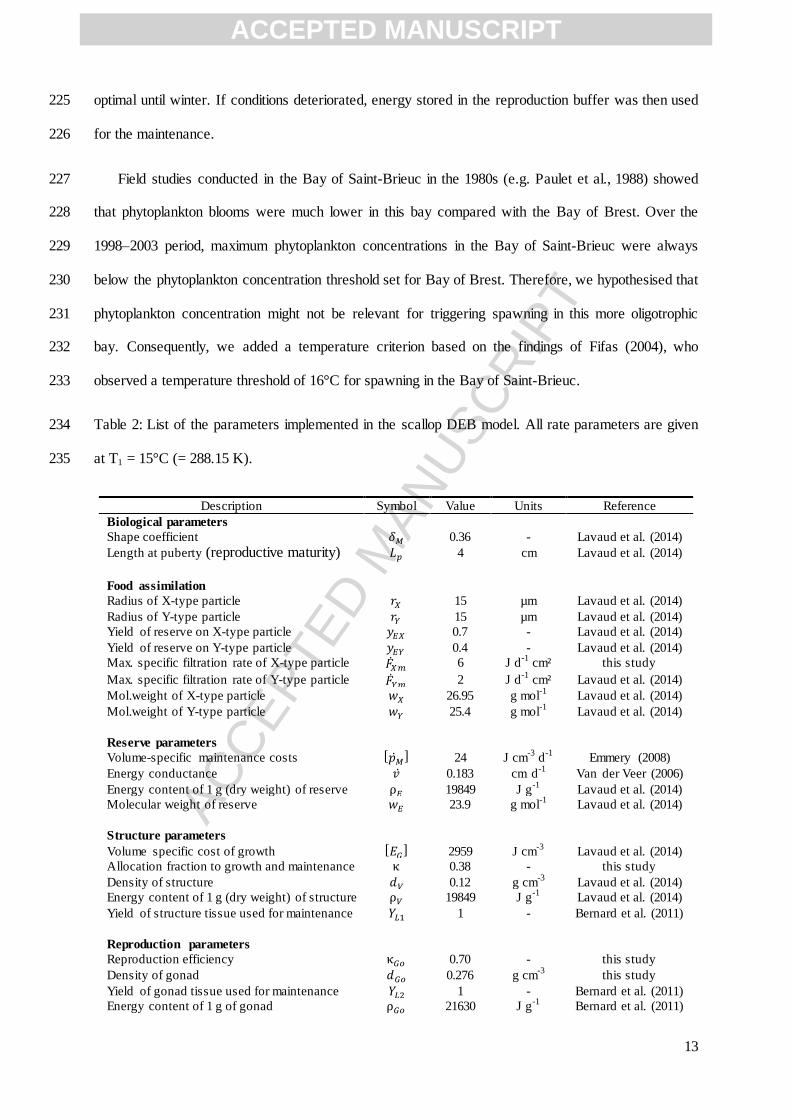
Table 2: List of the parameters implemented in the scallop DEB model. All rate parameters are given 234

at T1 = 15°C (= 288.15 K). 235

Description Symbol Value Units Reference

Biological parameters

Shape coefficient 0.36 - Lavaud et al. (2014)

Length at puberty (reproductive maturity) 4 cm Lavaud et al. (2014)

Food assimilation

Radius of X-type particle 15 µm Lavaud et al. (2014)

Radius of Y-type particle 15 µm Lavaud et al. (2014)

Yield of reserve on X-type particle 0.7 - Lavaud et al. (2014)

Yield of reserve on Y-type particle 0.4 - Lavaud et al. (2014)

Max. specific filtration rate of X-type particle ̇ 6 J d-1

cm² this study

Max. specific filtration rate of Y-type particle ̇ 2 J d-1

cm² Lavaud et al. (2014)

Mol.weight of X-type particle 26.95 g mol-1

Lavaud et al. (2014)

Mol.weight of Y-type particle 25.4 g mol-1

Lavaud et al. (2014)

Reserve parameters

Volume-specific maintenance costs [ ̇ ] 24 J cm-3

d-1

Emmery (2008)

Energy conductance ̇ 0.183 cm d-1

Van der Veer (2006)

Energy content of 1 g (dry weight) of reserve 19849 J g-1

Lavaud et al. (2014)

Molecular weight of reserve 23.9 g mol-1

Lavaud et al. (2014)

Structure parameters

Volume specific cost of growth [ ] 2959 J cm-3

Lavaud et al. (2014)

Allocation fraction to growth and maintenance 0.38 - this study

Density of structure 0.12 g cm-3

Lavaud et al. (2014)

Energy content of 1 g (dry weight) of structure 19849 J g-1

Lavaud et al. (2014)

Yield of structure tissue used for maintenance 1 - Bernard et al. (2011)

Reproduction parameters

Reproduction efficiency 0.70 - this study

Density of gonad 0.276 g cm-3

this study

Yield of gonad tissue used for maintenance 1 - Bernard et al. (2011)

Energy content of 1 g of gonad 21630 J g-1

Bernard et al. (2011)

ACCEPTED MANUSCRIPT

ACC

EPTE

D M

ANU

SCR

IPT

14

Temperature threshold for spawning 16 °C this study

Gonado-somatic index threshold for spawning 0.15 - this study

Temperature effect

Arrhenius temperature TA 8990 K Lavaud et al. (2014)

Lower boundary tolerance range 273.15 K Lavaud et al. (2014)

Arrhenius temperature for lower boundary 50000 K Lavaud et al. (2014)

236

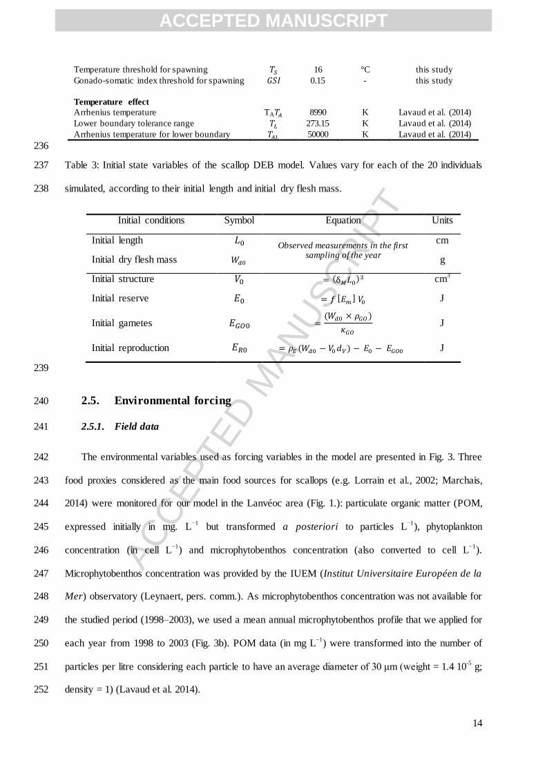
Table 3: Initial state variables of the scallop DEB model. Values vary for each of the 20 individuals 237

simulated, according to their initial length and initial dry flesh mass. 238

Initial conditions Symbol Equation Units

Initial length Observed measurements in the first

sampling of the year

cm

Initial dry flesh mass g

Initial structure ( ) cm

3

Initial reserve [ ] J

Initial gametes ( )

J

Initial reproduction ( ) J

239

2.5. Environmental forcing 240

2.5.1. Field data 241

The environmental variables used as forcing variables in the model are presented in Fig. 3. Three 242

food proxies considered as the main food sources for scallops (e.g. Lorrain et al., 2002; Marchais, 243

2014) were monitored for our model in the Lanvéoc area (Fig. 1.): particulate organic matter (POM, 244

expressed initially in mg. L−1

but transformed a posteriori to particles L−1

), phytoplankton 245

concentration (in cell L−1

) and microphytobenthos concentration (also converted to cell L−1

). 246

Microphytobenthos concentration was provided by the IUEM (Institut Universitaire Européen de la 247

Mer) observatory (Leynaert, pers. comm.). As microphytobenthos concentration was not available for 248

the studied period (1998–2003), we used a mean annual microphytobenthos profile that we applied for 249

each year from 1998 to 2003 (Fig. 3b). POM data (in mg L−1

) were transformed into the number of 250

particles per litre considering each particle to have an average diameter of 30 μm (weight = 1.4 10-5

g; 251

density = 1) (Lavaud et al. 2014). 252

ACCEPTED MANUSCRIPT

ACC

EPTE

D M

ANU

SCR

IPT

15

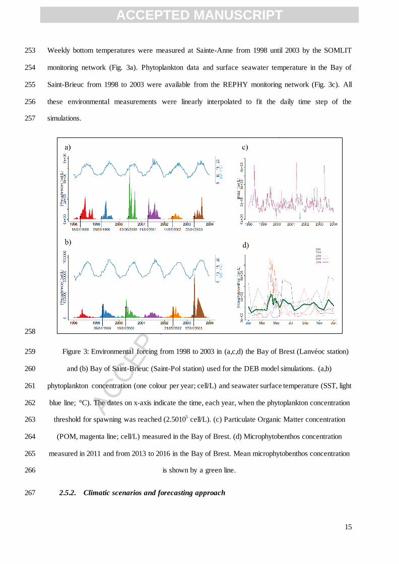
Weekly bottom temperatures were measured at Sainte-Anne from 1998 until 2003 by the SOMLIT 253

monitoring network (Fig. 3a). Phytoplankton data and surface seawater temperature in the Bay of 254

Saint-Brieuc from 1998 to 2003 were available from the REPHY monitoring network (Fig. 3c). All 255

these environmental measurements were linearly interpolated to fit the daily time step of the 256

simulations. 257

258

Figure 3: Environmental forcing from 1998 to 2003 in (a,c,d) the Bay of Brest (Lanvéoc station) 259

and (b) Bay of Saint-Brieuc (Saint-Pol station) used for the DEB model simulations. (a,b) 260

phytoplankton concentration (one colour per year; cell/L) and seawater surface temperature (SST, light 261

blue line; °C). The dates on x-axis indicate the time, each year, when the phytoplankton concentration 262

threshold for spawning was reached (2.50105 cell/L). (c) Particulate Organic Matter concentration 263

(POM, magenta line; cell/L) measured in the Bay of Brest. (d) Microphytobenthos concentration 264

measured in 2011 and from 2013 to 2016 in the Bay of Brest. Mean microphytobenthos concentration 265

is shown by a green line. 266

2.5.2. Climatic scenarios and forecasting approach 267

ACCEPTED MANUSCRIPT

ACC

EPTE

D M

ANU

SCR

IPT

16

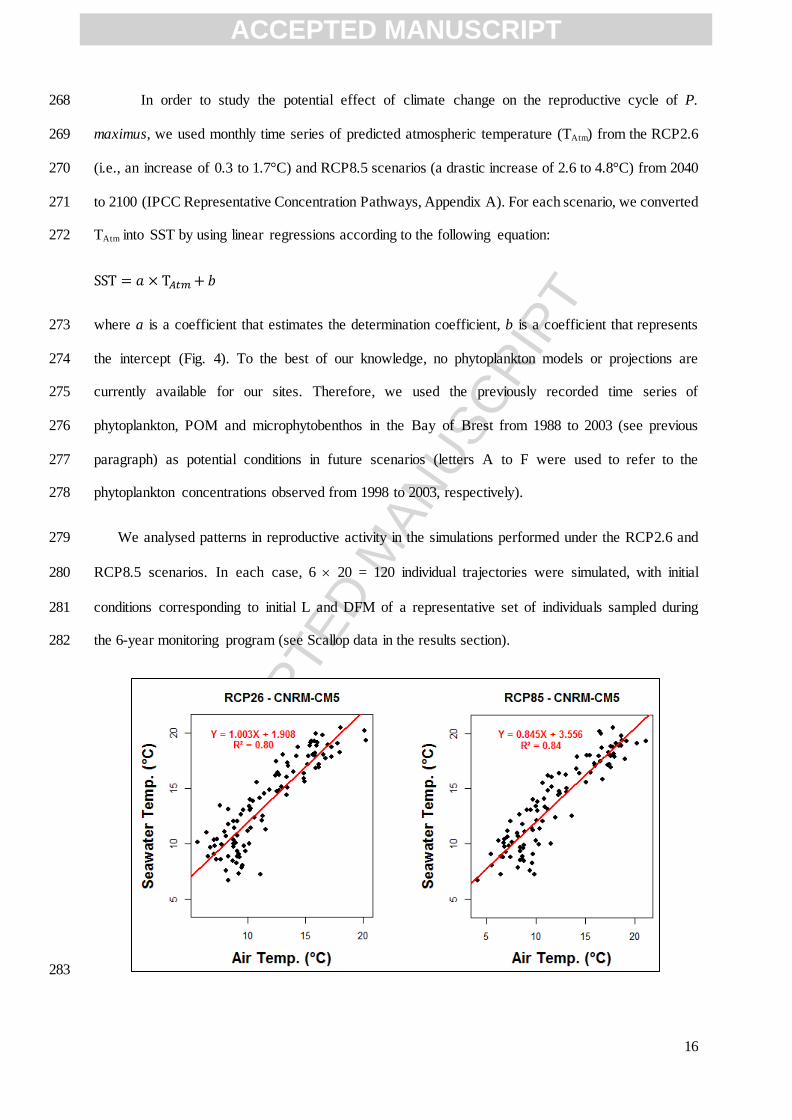
In order to study the potential effect of climate change on the reproductive cycle of P. 268

maximus, we used monthly time series of predicted atmospheric temperature (TAtm) from the RCP2.6 269

(i.e., an increase of 0.3 to 1.7°C) and RCP8.5 scenarios (a drastic increase of 2.6 to 4.8°C) from 2040 270

to 2100 (IPCC Representative Concentration Pathways, Appendix A). For each scenario, we converted 271

TAtm into SST by using linear regressions according to the following equation: 272

where a is a coefficient that estimates the determination coefficient, b is a coefficient that represents 273

the intercept (Fig. 4). To the best of our knowledge, no phytoplankton models or projections are 274

currently available for our sites. Therefore, we used the previously recorded time series of 275

phytoplankton, POM and microphytobenthos in the Bay of Brest from 1988 to 2003 (see previous 276

paragraph) as potential conditions in future scenarios (letters A to F were used to refer to the 277

phytoplankton concentrations observed from 1998 to 2003, respectively). 278

We analysed patterns in reproductive activity in the simulations performed under the RCP2.6 and 279

RCP8.5 scenarios. In each case, 6 20 = 120 individual trajectories were simulated, with initial 280

conditions corresponding to initial L and DFM of a representative set of individuals sampled during 281

the 6-year monitoring program (see Scallop data in the results section). 282

283

ACCEPTED MANUSCRIPT

ACC

EPTE

D M

ANU

SCR

IPT

17

Fig 4: Relations between monthly air temperature from the RCP scenarios and monthly seawater 284

temperature in the Bay of Brest (from 2006 to 2014): on the left, monthly air temperatures on monthly 285

seawater temperature under the RCP2.6 scenario with the CNRM-CM5 model; on the right, monthly 286

air temperatures on monthly seawater temperature under the RCP8.5 scenario with the CNRM-CM5 287

model. 288

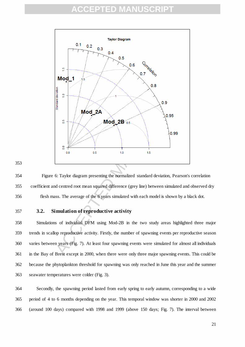
2.6. Statistical analysis 289

To evaluate the best fit, mean simulations for each model (Mod-1, Mod-2A and Mod-2B) and 290

mean observed data were compared using a Taylor diagram. This diagram provides a statistical 291

summary of the agreement between a reference (observed data) and modelling results (Taylor, 2001). 292

Three statistical measures are presented in the Taylor diagram: the centred root mean square (RMS) 293

difference, normalized standard deviation, and Pearson’s correlation coefficient. All statistical 294

analyses were conducted in R version 3.3.3 (R Core Team, 2017). 295

ACCEPTED MANUSCRIPT

ACC

EPTE

D M

ANU

SCR

IPT

18

3. Results 296

3.1. Contrasted environmental forcing conditions in the two study sites 297

Between 1998 and 2003, sea surface temperatures (SST) in the Bay of Brest reached a minimum 298

of 8.3°C in February 1998 and a maximum of 22.1°C in July 2001 (Fig 3a). The overall annual mean 299

was 14.0 ± 0.3°C. The warmest year was 2001, with a yearly mean temperature of 14.5°C. This year 300

also had the warmest summer, with a mean temperature of 18.4°C. The coldest year was 1998, with a 301

yearly mean temperature of 13.7°C. The coldest summer was 2000, with a mean temperature of 302

16.9°C. Phytoplankton concentration from 1998 to 2003 averaged 328,000 cell/L per year, with an 303

intra-annual SD of 135,000 cell/L. Phytoplankton concentration showed a seasonal pattern, with 304

maximum values in spring and summer and minimum values in winter (Fig 3a). The magnitude and 305

timing of spring and summer blooms showed high inter-annual variability. For example, the spring 306

bloom reached 5,000,000 cell/L in 2000, but the maximum phytoplankton concentration recorded in 307

2002 was 600,000 cell/L. The bloom onset date also differed among years. The first bloom observed 308

in 2000 (30,000 cell/L) occurred on 20 January, while it was observed on 25 February in 1998 309

(206,000 cell/L). 310

The POM concentration showed similar patterns over the study period (Fig. 3a). However, larger 311

peaks were observed in 1998, 2001 and 2003, at about 6,460,000 particles L-1

, compared with lower 312

values of 3,640,000 particles L-1

in 1999, 2000 and 2002. 313

Microphytobenthos concentration showed two seasonal trends (Fig. 3b). The first pattern was 314

observed in 2011 and 2013 with a large peak in spring and two smaller peaks in autumn and winter. 315

The second pattern, observed in 2014, 2015, and 2016, showed a peak in early summer and two 316

smaller ones in autumn and winter. The smallest number of microphytobenthic species (n = 22) were 317

identified in 2011 and a maximum of 67 species were identified in 2016. For the rest of the study, we 318

used a mean profile of microphytobenthos computed by taking the average of all these observations 319

(Fig. 3d). 320

ACCEPTED MANUSCRIPT

ACC

EPTE

D M

ANU

SCR

IPT

19

In the Bay of Saint-Brieuc, SST fluctuated between a minimum of 5.8°C in February 1998 and a 321

maximum of 21.2°C in July 2001 (Fig. 3b), thus showing a greater range of variation than the Bay of 322

Brest. The average SST was 12.6 ± 0.5°C. The warmest year was 2003 with a mean temperature of 323

13.6°C. This year also had the warmest summer with a mean temperature of 18.4°C. As in the Bay of 324

Brest, the coldest year was 1998, with a mean temperature of 12.6°C, and 2000 was the coldest 325

summer, with a mean temperature of 16.5°C. 326

Phytoplankton concentrations were maximal in spring and summer and minimal in winter (Fig 327

3b). The annual phytoplankton concentration from 1998 to 2003 averaged 40,764 ± 4,990 cell L-1

. 328

Bloom intensities were lower than in the Bay of Brest, but the magnitude and timing appeared quite 329

different from year to year. For example, the 2003 spring bloom peaked at 1,187,000 cell L-1

, while 330

only reaching 150,000 cell L-1

in 2001. The earliest first bloom was observed in 1999, on April 1 331

(114,000 cell L-1

), while the latest was observed in 2001, on May 14 (103,000 cell L-1

). 332

3.2. Comparing the DEB models 333

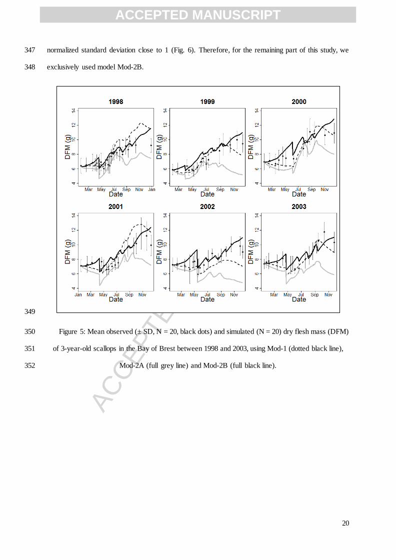
Simulations of dry flesh mass using model Mod-2A fitted the observations better than simulations 334

from Mod-1 (Fig. 5). The addition of the fourth state variable EGo seemed to improve prediction of 335

spawning events. Spawning events can be identified on each curve by a sharp decline in DFM. The 336

spawning period was more pronounced using Mod-2A than with Mod-1. For example, under Mod-1, 337

the first spawning occurred on May 11 in 1999 whereas it appeared March 28 under Mod-2A. 338

However, neither model successfully reproduced the observed increase in DFM from March to May. 339

On average, the difference between observed and simulated DFM values from January to May was ± 340

0.39 g under Mod-1 and ± 0.95 g under Mod-2A. DFM modelled using Mod-2B was more accurate 341

and the increase of DFM in spring fitted the observed data well (± 0.09 g of difference). Similarly to 342

Mod-2A, the spawning period was longer and more realistic than when using Mod-1. The addition of 343

microphytobenthos to phytoplankton for P. maximus food intake allowed a better simulation of growth 344

and reproductive activity, especially in the spring. For all years, model Mod-2B gave the best fit 345

between observations and simulations of growth, with a mean correlation coefficient up to 0.9 and a 346

ACCEPTED MANUSCRIPT

ACC

EPTE

D M

ANU

SCR

IPT

20

normalized standard deviation close to 1 (Fig. 6). Therefore, for the remaining part of this study, we 347

exclusively used model Mod-2B. 348

349

Figure 5: Mean observed (± SD, N = 20, black dots) and simulated (N = 20) dry flesh mass (DFM) 350

of 3-year-old scallops in the Bay of Brest between 1998 and 2003, using Mod-1 (dotted black line), 351

Mod-2A (full grey line) and Mod-2B (full black line). 352

ACCEPTED MANUSCRIPT

ACC

EPTE

D M

ANU

SCR

IPT

21

353

Figure 6: Taylor diagram presenting the normalized standard deviation, Pearson's correlation 354

coefficient and centred root mean squared difference (grey line) between simulated and observed dry 355

flesh mass. The average of the 6 years simulated with each model is shown by a black dot. 356

3.2. Simulation of reproductive activity 357

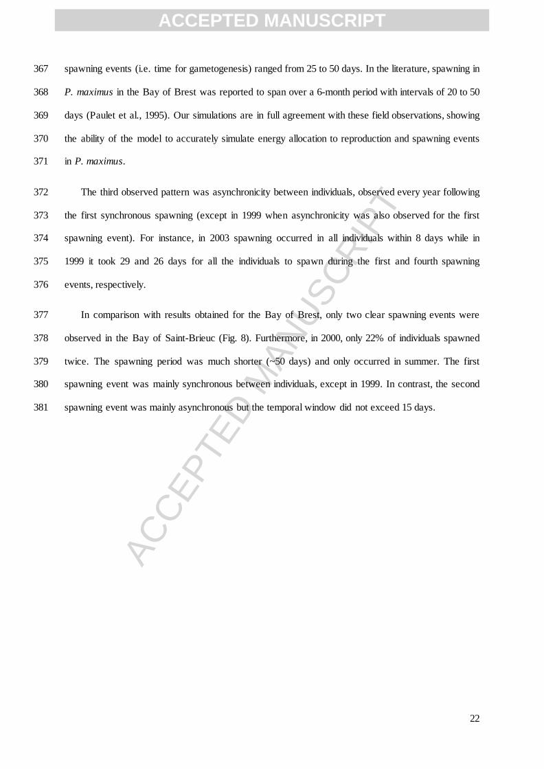
Simulations of individual DFM using Mod-2B in the two study areas highlighted three major 358

trends in scallop reproductive activity. Firstly, the number of spawning events per reproductive season 359

varies between years (Fig. 7). At least four spawning events were simulated for almost all individuals 360

in the Bay of Brest except in 2000, when there were only three major spawning events. This could be 361

because the phytoplankton threshold for spawning was only reached in June this year and the summer 362

seawater temperatures were colder (Fig. 3). 363

Secondly, the spawning period lasted from early spring to early autumn, corresponding to a wide 364

period of 4 to 6 months depending on the year. This temporal window was shorter in 2000 and 2002 365

(around 100 days) compared with 1998 and 1999 (above 150 days; Fig. 7). The interval between 366

ACCEPTED MANUSCRIPT

ACC

EPTE

D M

ANU

SCR

IPT

22

spawning events (i.e. time for gametogenesis) ranged from 25 to 50 days. In the literature, spawning in 367

P. maximus in the Bay of Brest was reported to span over a 6-month period with intervals of 20 to 50 368

days (Paulet et al., 1995). Our simulations are in full agreement with these field observations, showing 369

the ability of the model to accurately simulate energy allocation to reproduction and spawning events 370

in P. maximus. 371

The third observed pattern was asynchronicity between individuals, observed every year following 372

the first synchronous spawning (except in 1999 when asynchronicity was also observed for the first 373

spawning event). For instance, in 2003 spawning occurred in all individuals within 8 days while in 374

1999 it took 29 and 26 days for all the individuals to spawn during the first and fourth spawning 375

events, respectively. 376

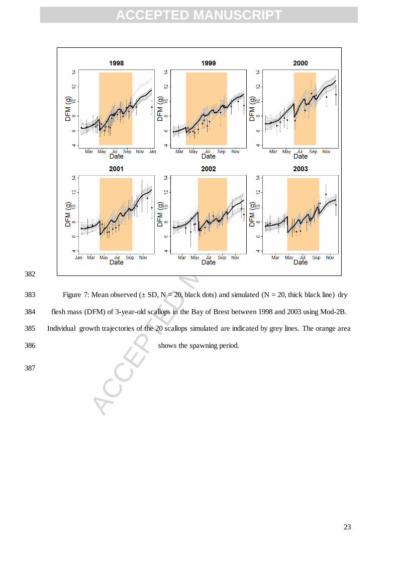
In comparison with results obtained for the Bay of Brest, only two clear spawning events were 377

observed in the Bay of Saint-Brieuc (Fig. 8). Furthermore, in 2000, only 22% of individuals spawned 378

twice. The spawning period was much shorter (~50 days) and only occurred in summer. The first 379

spawning event was mainly synchronous between individuals, except in 1999. In contrast, the second 380

spawning event was mainly asynchronous but the temporal window did not exceed 15 days. 381

ACCEPTED MANUSCRIPT

ACC

EPTE

D M

ANU

SCR

IPT

23

382

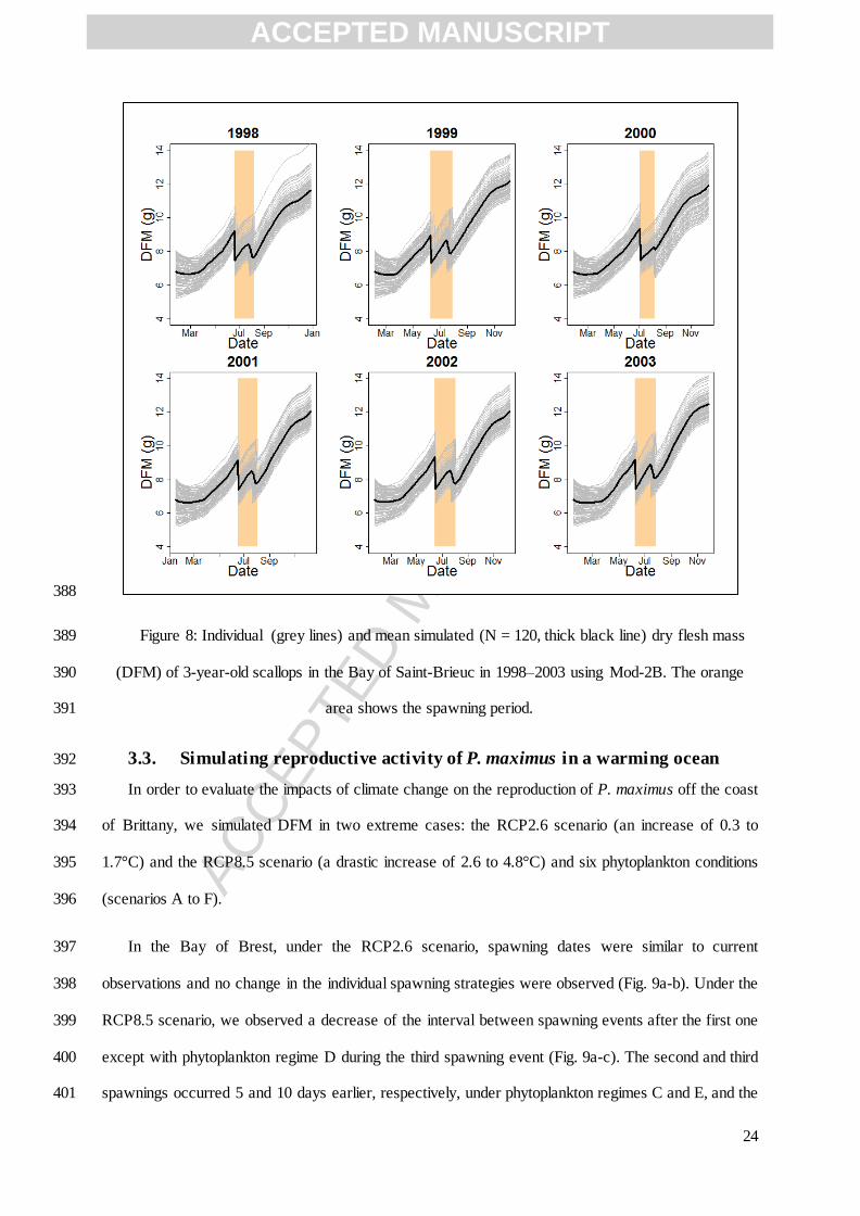
Figure 7: Mean observed (± SD, N = 20, black dots) and simulated (N = 20, thick black line) dry 383

flesh mass (DFM) of 3-year-old scallops in the Bay of Brest between 1998 and 2003 using Mod-2B. 384

Individual growth trajectories of the 20 scallops simulated are indicated by grey lines. The orange area 385

shows the spawning period. 386

387

ACCEPTED MANUSCRIPT

ACC

EPTE

D M

ANU

SCR

IPT

24

388

Figure 8: Individual (grey lines) and mean simulated (N = 120, thick black line) dry flesh mass 389

(DFM) of 3-year-old scallops in the Bay of Saint-Brieuc in 1998–2003 using Mod-2B. The orange 390

area shows the spawning period. 391

3.3. Simulating reproductive activity of P. maximus in a warming ocean 392

In order to evaluate the impacts of climate change on the reproduction of P. maximus off the coast 393

of Brittany, we simulated DFM in two extreme cases: the RCP2.6 scenario (an increase of 0.3 to 394

1.7°C) and the RCP8.5 scenario (a drastic increase of 2.6 to 4.8°C) and six phytoplankton conditions 395

(scenarios A to F). 396

In the Bay of Brest, under the RCP2.6 scenario, spawning dates were similar to current 397

observations and no change in the individual spawning strategies were observed (Fig. 9a-b). Under the 398

RCP8.5 scenario, we observed a decrease of the interval between spawning events after the first one 399

except with phytoplankton regime D during the third spawning event (Fig. 9a-c). The second and third 400

spawnings occurred 5 and 10 days earlier, respectively, under phytoplankton regimes C and E, and the 401

ACCEPTED MANUSCRIPT

ACC

EPTE

D M

ANU

SCR

IPT

25

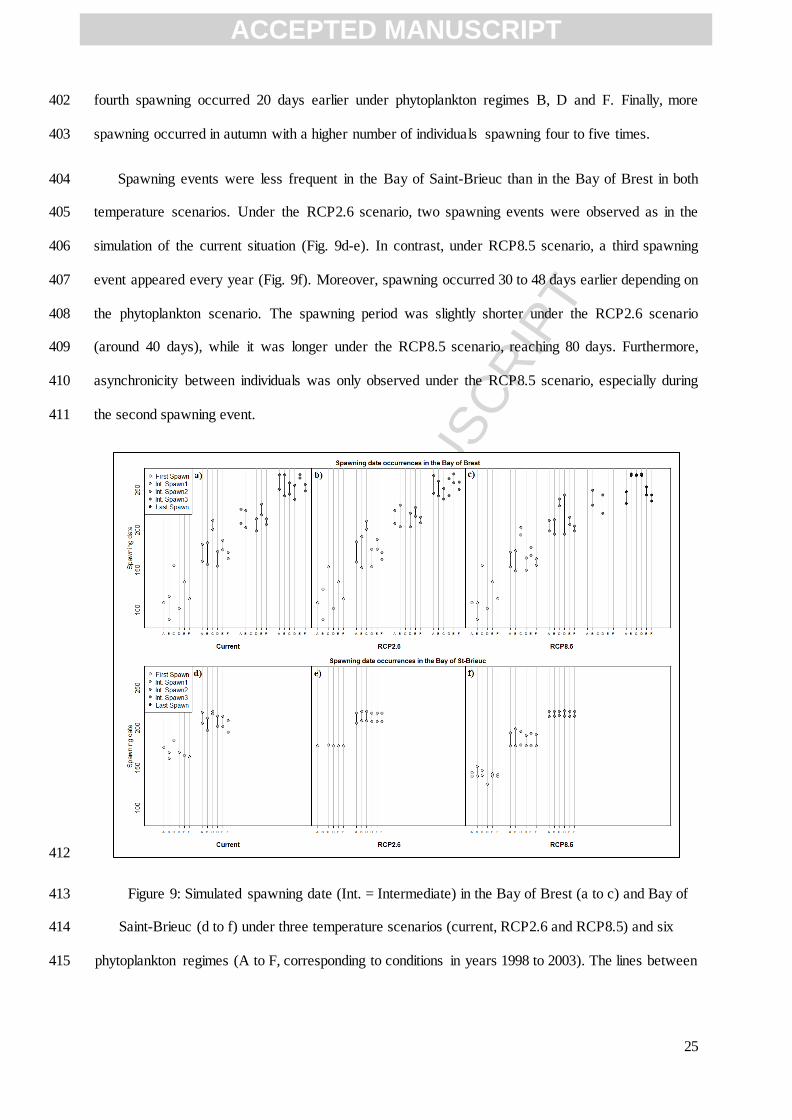
fourth spawning occurred 20 days earlier under phytoplankton regimes B, D and F. Finally, more 402

spawning occurred in autumn with a higher number of individuals spawning four to five times. 403

Spawning events were less frequent in the Bay of Saint-Brieuc than in the Bay of Brest in both 404

temperature scenarios. Under the RCP2.6 scenario, two spawning events were observed as in the 405

simulation of the current situation (Fig. 9d-e). In contrast, under RCP8.5 scenario, a third spawning 406

event appeared every year (Fig. 9f). Moreover, spawning occurred 30 to 48 days earlier depending on 407

the phytoplankton scenario. The spawning period was slightly shorter under the RCP2.6 scenario 408

(around 40 days), while it was longer under the RCP8.5 scenario, reaching 80 days. Furthermore, 409

asynchronicity between individuals was only observed under the RCP8.5 scenario, especially during 410

the second spawning event. 411

412

Figure 9: Simulated spawning date (Int. = Intermediate) in the Bay of Brest (a to c) and Bay of 413

Saint-Brieuc (d to f) under three temperature scenarios (current, RCP2.6 and RCP8.5) and six 414

phytoplankton regimes (A to F, corresponding to conditions in years 1998 to 2003). The lines between 415

ACCEPTED MANUSCRIPT

ACC

EPTE

D M

ANU

SCR

IPT

26

two points represent the asynchronicity between individuals with the first and last spawning date 416

within a population. 417

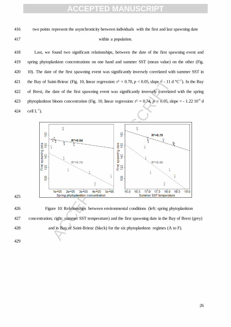
Last, we found two significant relationships, between the date of the first spawning event and 418

spring phytoplankton concentrations on one hand and summer SST (mean value) on the other (Fig. 419

10). The date of the first spawning event was significantly inversely correlated with summer SST in 420

the Bay of Saint-Brieuc (Fig. 10, linear regression: r² = 0.70, p < 0.05, slope = - 11 d °C-1

). In the Bay 421

of Brest, the date of the first spawning event was significantly inversely correlated with the spring 422

phytoplankton bloom concentration (Fig. 10, linear regression: r² = 0.74, p < 0.05, slope = - 1.22 10-4

d 423

cell L-1

). 424

425

Figure 10: Relationships between environmental conditions (left: spring phytoplankton 426

concentration; right: summer SST temperature) and the first spawning date in the Bay of Brest (grey) 427

and in Bay of Saint-Brieuc (black) for the six phytoplankton regimes (A to F). 428

429

ACCEPTED MANUSCRIPT

ACC

EPTE

D M

ANU

SCR

IPT

27

4. Discussion 430

The main objective of this study was to quantify the influence of environmental variables 431

(temperature and food sources) on the reproductive processes of the great scallop, P. maximus, and 432

explore the potential impacts of climate change on its dynamics. We improved an existing scallop 433

DEB model developed by Lavaud et al. (2014) by detailing the reproductive processes and by adding 434

microphytobenthos as a new food source. 435

In order to improve the DEB model for P. maximus, a fourth state variable was added to describe 436

the fixation of energy in gametes, as done by Bernard et al. (2011) for the Pacific oyster, Crassostrea 437

gigas. Furthermore, the maximum possible shell length was assumed to be 20 cm rather than the 438

previous assumption of 12 cm, since studies have shown that adult scallops can reach 16 cm in the 439

most favourable conditions (Mason, 1957; Chauvaud et al., 2012) and thus the ultimate length would 440

presumably be above 16 cm. This led to the recalculation of three model parameters:{ ̇ }, [ ̇ ] and 441

. The new values obtained are different from the previous version in Lavaud et al. (2014), particularly 442

. The previous value, fixed at 0.86, was high compared with other bivalve species. For instance, the 443

value for Crassostrea gigas is around 0.45. Considering that, in some environments, P. maximus could 444

spawn more than three times within the same reproductive season and that its gonad represents more 445

than 30 % of the whole flesh weight at maturity, it seems logical that this species would have a high 446

energy allocation ratio (and thus a low value for κ) similarly to C. gigas. Considering this, the new 447

value calculated here is probably more consistent with the reproductive capacity of P. maximus. These 448

changes do not fundamentally alter the dynamics of the model, but allow more spawning events and 449

higher fecundity than other versions of the model. Of course, further testing in other locations with 450

contrasted forcing conditions as well as with younger age-classes would also be needed to fully 451

validate this updated version of the scallop DEB model. 452

Another improvement made in the current model concerns trophic resources. Microphytobenthos 453

was added as a new source of food for scallops. Previously, Lavaud et al. (2014) demonstrated that 454

POM constitutes an additional food source allowing scallops to compensate phytoplankton limitation. 455

In addition, our study suggests that microphytobenthos would probably also be a valuable source of 456

ACCEPTED MANUSCRIPT

ACC

EPTE

D M

ANU

SCR

IPT

28

food that could sustain energy acquisition, especially in spring. For the moment, the taxonomic 457

composition of each food source is not detailed in the model, but several studies have shown 458

relationships between specific phytoplankton species and life history traits of the great scallop in 459

Brittany. For example, Chauvaud et al. (1998, 2001) showed, in the Bay of Brest, that growth and food 460

intake of P. maximus were dependent on phytoplankton taxonomic composition and concentration. 461

The related growth cessation depended on massive sedimentation of diatom blooms or toxic 462

dinoflagellate blooms. For example, P. maximus food intake and growth were highest when 463

Cerataulina pelagica blooms occurred and lowest during Gymnodinium nagasakiense blooms. In 464

addition, Lorrain et al. (2000) demonstrated that large bottom concentrations of chlorophyll-a, 465

following diatom blooms, could have a negative effect on the ingestion or respiration of P. maximus 466

juveniles, either by gill clogging or by oxygen depletion at the water-sediment interface associated 467

with the degradation of organic matter. The current version of the DEB model does not take into 468

account these specific effects which are linked to the type of food that is available. However the 469

current model provides the basis for taking them into consideration in future studies. 470

One major difficulty with a modelling approach is to obtain a sufficient dataset to calibrate, test 471

and validate a numerical model. When using a bioenergetics model, this implies monitoring growth 472

and reproduction of marine organisms and their surrounding environmental data, at the same place and 473

ideally over a long period (many years) to evaluate temporal phenotypic variability. In our study, the 474

Bay of Brest sampling sites (St Anne, Roscanvel, Lanvéoc) are not closed off from each other but are 475

instead located in a very well mixed area within the Bay of Brest (Salomon and Breton, 1991) where 476

scallops are the most abundant. So we can suppose that environmental data are sufficiently 477

representative of conditions encountered by scallops. In the Bay of Saint Brieuc, there is no growth 478

monitoring of scallops and there are too many gaps in the environmental data to apply the model in a 479

satisfactory manner. Our approach is therefore limited but it offers a first application of the model to 480

this new environment and constitutes a stepping-stone for further development of the modelling 481

approach for this bay. 482

ACCEPTED MANUSCRIPT

ACC

EPTE

D M

ANU

SCR

IPT

29

Other limitations of our model that should be mentioned are its systematic overestimation of 483

growth during the autumnal period and an insufficient integration of inter-individual variability. The 484

systematic tendency to overestimate growth could be due to a change in the physiology of scallops at 485

the end of the reproductive season and period leading into winter. Specific ecophysiological 486

experiments should be developed to address this question and improve the model. For the moment, we 487

have applied an individual-based modelling strategy by introducing variability between individuals 488

through the initial condition values. To account for more variability in physiological traits, similar 489

studies, e.g. Thomas et al. (2015) and Bacher and Gangnery (2006) used specific model 490

parameterization of the ingestion function for each individual. For instance, Xk values were allocated 491

to each individual following a Gaussian distribution. It would now be interesting to adapt a similar 492

approach to the scallop DEB model. 493

Quantitative modelling of reproductive processes (preliminary storage phase, gametogenesis, 494

spawning and/or resorption) is not easy as these processes are typically species-specific. There are no 495

general rules on how to handle reproductive activity in DEB theory, especially regarding reproduction 496

buffer dynamics. Bernard et al. (2011) introduced a fourth state variable in order to improve modelling 497

of reproduction dynamics in the Pacific oyster, Crassostrea gigas. Numerous marine organisms from 498

temperate waters spawn once or twice at a relatively fixed time each year (Gosling, 2004). For P. 499

maximus, however, reproductive activity is more complex, with asynchronous spawning during a 500

highly variable reproductive window. For this preliminary approach, however, we made the 501

assumption that the mechanisms governing reproductive activity would be quite similar among 502

bivalves and thus between oysters and scallops. 503

The reproductive cycle of P. maximus has been studied extensively in many places (e.g. Magnesen 504

and Christophersen, 2008). Concerning our studied area, contrasting patterns were shown between the 505

Bay of Brest and Bay of Saint-Brieuc (Paulet et al., 1995). Scallops in the Bay of Brest usually spawn 506

between April and October, with a massive first spawning in April followed by a second maturation 507

phase until July characterized by one or several smaller spawning events. A third summer maturation 508

phase leads to a last major spawning event during August (Paulet et al., 1995). A late spawning event 509

ACCEPTED MANUSCRIPT

ACC

EPTE

D M

ANU

SCR

IPT

30

may be observed in autumn, but only in a few individuals (Saout et al., 2000). In the Bay of Brest, this 510

seasonal cycle varies strongly between individuals, resulting in a lack of synchronism (Paulet et al., 511

1995). The results from our simulations, obtained over six years in the Bay of Brest, correspond fairly 512

well to this description. More precisely, the model was able to partly simulate the observed 513

asynchronicity between individuals, and the mechanisms implemented to trigger spawning appeared to 514

be sufficiently relevant to simulate the onset of the first spawning, the temporal spawning window, 515

and the number of spawning events (Fig. 6). 516

In the Bay of Saint-Brieuc, scallops only spawn from June until mid-August (Paulet et al., 1988; 517

Paulet, 1990). Moreover, the seasonal cycle is known to be similar between individuals, showing a 518

higher synchronism in this area than in the Bay of Brest (Paulet et al., 1988). Of course, the 519

application of our model in the Bay of Saint-Brieuc is only a first attempt and suffers from a lack of 520

forcing data. Nevertheless, it seems that the current version of the model was able to reproduce the 521

different patterns of the reproductive cycle of P. maximus observed in this area. This tends to confirm 522

that the environmental factors used here are the main key-drivers of reproduction processes of P. 523

maximus. 524

Despite its limitations, our modelling study suggests that differences in the timing of spawning 525

events might be explained mainly by environmental differences in food and temperature. Among 526

invertebrates, there is much evidence for the influence of exogenous factors (e.g. temperature, food 527

and photoperiod) on the progress of gametogenesis and for regulation by endogenous rhythms on 528

which environmental signals may act as synchronizers (e.g. Mat et al., 2014). Many environmental 529

variables trigger such regulation but, most often, temperature and food availability (Franco et al., 530

2015; Ubertini et al., 2017) are considered to be the key factors. This is the case for bivalves, 531

particularly pectinids (Lavaud et al. 2014). Scallops are sublittoral, epifaunal and active suspension-532

feeding bivalves that rely on suspended detrital material, phytoplankton and microphytobenthos as 533

their main food sources (Robert et al., 1994; Chauvaud et al., 2001). Saout et al. (1999) showed that, 534

in P. maximus, a simultaneous increase of temperature and photoperiod enhanced gonad growth when 535

food is not limiting. However, it was still not clear which of these two factors is the more influential. 536

ACCEPTED MANUSCRIPT

ACC

EPTE

D M

ANU

SCR

IPT

31

Our results obtained in the Bay of Brest show that, within a temporal photoperiod window, spawning 537

is mainly triggered mainly by phytoplankton blooms once the GSI threshold is reached. In this 538

eutrophic area, temperature might play a secondary role in terms of triggering spawning. For instance, 539

in 2000 and 2002, the first bloom of the year was late compared with the other years (June 3 and May 540

14, respectively; Fig. 3). Accordingly, for both years, the model simulated a later occurrence of first 541

spawning (June 4 and May 15, respectively; Fig. 7) that fitted well with field observations. By 542

comparison, blooms of phytoplankton in the Bay of Saint-Brieuc were much lower than those 543

observed in the Bay of Brest and presumably not a source of stress. Values were always below the 544

threshold for triggering spawning. In this new environment, phytoplankton blooms were presumably 545

not the trigger for spawning. Based on previous studies, we basically used a temperature threshold in 546

this environment (Fifas, 2004) and the simulations obtained were in accordance with spawning 547

processes observed in this bay. 548

In the last part of this study, we explored the potential consequences of climate change for the 549

reproductive activity of P. maximus in northern Brittany. Predicting the temperature of the future 550

atmosphere and oceans has been a focus of research for a few decades now. The evolution of food 551

supply to organisms, which in the ocean starts with phytoplankton, is comparatively less well 552

understood or predictable. Although the reliability of ocean primary production models is continually 553

improving, predicting the future is challenging (Gradinger et al.,2009; Lavoie et al., 2017) for coastal 554

environments. In this context, we believe that our approach, consisting of transposing current food 555

availability time series to future scenarios, is valuable because it allows a greater degree of complexity 556

in predictions as it provides realistic estimates of inter-annual variability. This approach could be 557

complemented by simulations under enhanced phytoplankton productivity, as predicted by recent 558

modelling (Jensen et al., 2017). Only the most extreme scenario (RCP8.5) revealed contrasting 559

predictions with the current one. While distinct reproductive cycles are currently observed between the 560

Bay of Brest and the Bay of Saint-Brieuc, it seems that future environmental conditions would 561

generally extend the spawning period, with an additional spawning event predicted in both locations. 562

However, contrasted impacts also emerged when comparing simulations obtained for the two bays. An 563

ACCEPTED MANUSCRIPT

ACC

EPTE

D M

ANU

SCR

IPT

32

increase in seawater temperature advanced the onset of spawning by 20 to 44 days in the Bay of Saint-564

Brieuc, irrespective of the phytoplankton scenario, while the spawning timeline in the Bay of Brest 565

was unchanged. Warmer temperatures might also lead to better recruitment. Shephard et al. (2010) 566

found that the mean annual recruitment of young scallops in the Isle of Man was positively related to 567

spring water temperature. Adult gonads were also larger, indicating higher egg production during 568

warmer years. Our simulations led to similar conclusions, showing that an increase in seawater 569

temperature combined with adequate food supply could well enhance scallop recruitment by: (1) 570

increasing the spawning window in late summer and (2) advancing the onset of spawning in spring in 571

the Bay of Saint-Brieuc. 572

ACCEPTED MANUSCRIPT

ACC

EPTE

D M

ANU

SCR

IPT

33

Acknowledgements 573

A grant from Région Bretagne and the University of Western Brittany (UBO) supported MG 574

during her PhD work. The authors are grateful to the IUEM staff of the EVECOS networks, the 575

IFREMER staff of the REPHY network and the staff of the SOMLIT network, through which all the 576

field data were gathered. We also thank Helen McCombie-Boudry of the Translation Bureau of the 577

University of Western Brittany for improving the English of this manuscript. 578

579

ACCEPTED MANUSCRIPT

ACC

EPTE

D M

ANU

SCR

IPT

34

References 580

Alunno-Bruscia, M., Bourlès, Y., Maurer, D., Robert, S., Mazurié, J., Gangnery, A., Goulletquer, 581

P.,Pouvreau, S. (2011). A single bio-energetics growth and reproduction model for the oyster 582

Crassostrea gigas in six Atlantic ecosystems. J. Sea Res. 66, 340–348. 583

Ansell, A. D. (1991). Three European scallops: Pecten maximus, Chlamys (Aequipecten) opercularis 584

and C.(Chlamys) varia. Scallops: Biology, Ecology and Aquaculture, 715-751. 585

Bacher, C. & Gangnery, A. (2006). Use of Dynamic Energy Budget and Individual Based models to 586

simulate the dynamics of cultivated oyster populations. J. Sea Res. 56, 140–155. 587

http://doi:10.1016/j.seares.2006.03.004 588

Bayne, B. L., Hawkins, A. J. S., & Navarro, E. (1987). Feeding and digestion by the mussel Mytilus 589

edulis L.(Bivalvia: Mollusca) in mixtures of silt and algal cells at low concentrations. Journal of 590

Experimental Marine Biology and Ecology, 111(1), 1-22. 591

Belin, C. and co-authors (2017). REPHY – French Observation and Monitoring program for 592

Phytoplankton and Hydrology in coastal waters (2017). REPHY dataset - French Observation and 593

Monitoring program for Phytoplankton and Hydrology in coastal waters. 1987-2016 Metropolitan 594

data. SEANOE. http://doi.org/10.17882/47248 595

Bernard, I., de Kermoysan, G., Pouvreau, S. (2011). Effect of phytoplankton and temperature on the 596

reproduction of the Pacific oyster Crassostrea gigas: investigation through DEB theory. J. Sea 597

Res. 66, 349–360. 598

Beukema, J. J., Dekker, R., Jansen, J. M. (2009). Some like it cold: populations of the tellinid bivalve 599

Macoma balthica (L.) suffer in various ways from a warming climate. Marine Ecology Progress 600

Series, 384, 135-145. 601

Chauvaud, L., Thouzeau, G., Paulet, Y.M. (1998). Effects of environmental factors on the daily 602

growth rate of Pecten maximus juveniles in the Bay of Brest (France). J. Exp. Mar. Biol. Ecol. 603

227, 83–111. 604

Chauvaud, L., Donval, A., Thouzeau, G., Paulet, Y.M., Nézan, E. (2001). Variations in food intake of 605

Pecten maximus (L.) from the Bay of Brest (France): influence of environmental factors and 606

phytoplankton species composition. C. R. Acad. Sci. III 324, 743–755. 607

Chauvaud, L., Patry, Y., Jolivet, A., Cam, E., Le Goff, C., Strand, Ø., Charrier, G., Thébault, J., 608

Lazure, P., Gotthard, K., Clavier, J. (2012). Variation in size and growth of the great scallop 609

Pecten maximus along a latitudinal gradient. PLoS ONE 7, e37717. 610

ACCEPTED MANUSCRIPT

ACC

EPTE

D M

ANU

SCR

IPT

35

Claereboudt, M. R., & Himmelman, J. H. (1996). Recruitment, growth and production of giant 611

scallops (Placopecten magellanicus) along an environmental gradient in Baie des Chaleurs, 612

eastern Canada. Marine Biology, 124(4), 661-670. 613

Devauchelle, N., & Mingant, C. (1991). Review of the reproductive physiology of the scallop, Pecten 614

maximus, applicable to intensive aquaculture. Aquatic Living Resources, 4(1), 41-51. 615

Emmery, A. (2008). Modélisation de la croissance et de la reproduction de la coquille Saint-Jacques 616

Pecten maximus selon la théorie «Dynamic Energy Budget» : variabilité environnementale et 617

croissance individuelle. Univeristy of Western Brittany (Master thesis). 618

Fifas, S. (2004). La coquille Saint-Jacques en Bretagne. Rapport Ifremer. Direction des Ressources 619

Vivantes. Ressources Halieutiques. 14p. 620

Foveau A., Foucher E., Desroy N., (2013). Identification biogéographique des gisements de coquilles 621

Saint-Jacques en Manche. Réunion finale du projet ANR CoManche. Caen, France. 10-11 622

décembre 2013. 623

Franco, C., Aldred, N., Sykes, A. V., Cruz, T., Clare, A. S (2015). The effects of rearing temperature 624

on reproductive conditioning of stalked barnacles (Pollicipes pollicipes). Aquaculture, vol 448, 625

410-417. Doi:10.1016/j.aquaculture.2015.06.015 626

Gosling, E. (2004). Bivalve Molluscs. Biology, Ecology and Culture. Edition Fishing News Books. 627

444p. 628

Gourault, M., Petton, S., Thomas, Y., Pecquerie, L., Marques, G.M., Cassou, C., Fleury, E., Paulet, Y-629

M., Pouvreau, S (submitted, this issue). Modelling reproductive traits of an invasive bivalve 630

species under contrasted climate scenarios from 1960 to 2100. Journal of Sea Research. 631

Gradinger, R. (2009). Sea-ice algae: Major contributors to primary production and algal biomass in the 632

Chukchi and Beaufort Seas during May/June 2002. Deep Sea Research Part II: Topical Studies in 633

Oceanography, 56(17), pp.1201-1212. 634

Guerin, L. (2004). La crépidule en Rade de Brest: un modèle biologique d’espèce introduite 635

proliférante en réponse aux fluctuations de l’environnement. University of Western Brittany (PhD 636

thesis). 637

ICES, (2015). Report of the Scallop Assessment Working Group (WGScallop), 6-10 October 2014, 638

Nantes, France. ICES CM 2014\ACOM:24. 35 pp. 639

IPCC, (2014). Climate Change 2014: Synthesis Report. Contribution of Working Groups I, II and III 640

to the Fifth Assessment Report of the Intergovernmental Panel on Climate Change [Core Writing 641

Team, R.K. Pachauri and L.A. Meyer (eds.)]. IPCC, Geneva, Switzerland, 151 pp. 642

ACCEPTED MANUSCRIPT

ACC

EPTE

D M

ANU

SCR

IPT

36

Jensen, L.Ø., Mousing, E.A. and Richardson, K. (2017). Using species distribution modelling to 643

predict future distributions of phytoplankton: Case study using species important for the 644

biological pump. Marine Ecology, 38(3). 645

Kooijman, S.A.L.M. (2010). Dynamic Energy Budget Theory for Metabolic Organization. Cambridge 646

Ed., University Press, Cambridge, UK. 647

Lavaud, R., Flye-Sainte-Marie, J., Jean, F., Emmery, A., Strand, O., Kooijman, S.A.L.M. (2014). 648

Feeding and energetics of the great scallop, Pecten maximus, through a DEB model. Journal of 649

Sea Research, vol 94, 5-18. 650

Lavoie, D., Lambert, N. and Gilbert, D. (2017). Projections of Future Trends in Biogeochemical 651

Conditions in the Northwest Atlantic Using CMIP5 Earth System Models. Atmosphere-Ocean, 652

pp.1-23. 653

Leynaert, A. (2016). Observatoire de l’Institut Universitaire et Européen de la Mer, série Microalgues. 654

https://www-iuem.univ-brest.fr/observatoire/observation-cotiere/faune-flore/microalgues 655

Lorrain, A., Paulet, Y.M., Chauvaud, L., Savoye, N., Nézan, E., Guérin, L. (2000). Growth anomalies 656

in from coastal waters (Bay of Brest, France): relationship with diatom blooms. J. Mar. Biol. 657

Assoc. UK 80, 667–673. 658

Lorrain, A., Paulet, Y.M., Chauvaud, L., Savoye, N., Donval, A., Saout, C. (2002). Differential δ13C 659

and δ15N signatures among scallop tissues: implications for ecology and physiology. J. Exp. Mar. 660

Biol. Ecol. 275, 47–61. 661

Magnesen, T. & Christophersen, G. (2008). Reproductive cycle and conditioning of translocated 662

scallops (Pecten maximus) from five broodstock populations in Norway. Aquaculture, 285(1), 663

109-116. 664

Marchais, V. (2014). Relations trophiques entre producteurs primaires et quatre consommateurs 665

primaires benthiques dans un écosystème côtier tempéré. University of Western Brittany (PhD 666

thesis). 667

Mason, J. (1957). The age and growth of the scallop, Pecten maximus (L.), in Manx waters. J. Mar. 668

Biol. Assoc. U. K. 36, 473–492. 669

Mat, A., Massabuau, J.C., Ciret, P., Tran, D. (2014). Looking for the clock mechanism responsible for 670

circatidal behavior in the oyster Crassostrea gigas. Marine Biology, vol 161, issue 1, 89-99. 671

Menge, B.A., Chan, F., Nielsen, K.J., Lorenzo, E.D. & Lubchenco, J. (2009) Climatic variation alters 672

supply-side ecology: impact of climate patterns on phytoplankton and mussel recruitment. 673

Ecological Monographs, 79, 379–395. doi:10.1890/08-2086.1 674

ACCEPTED MANUSCRIPT

ACC

EPTE

D M

ANU

SCR

IPT

37

Montalto, V., Martinez, M., Rinaldi, A., Sarà, G. & Mirto, S. (2017). The effect of the quality of diet 675

on the functional response of Mytilus galloprovincialis (Lamarck, 1819): Implications for 676

integrated multitrophic aquaculture (IMTA) and marine spatial planning. Aquaculture 468, 371–677

377. doi:10.1016/j.aquaculture.2016.10.030 678

Morgan, E., O’ Riordan, R.M. & Culloty, S.C. (2013) Climate change impacts on potential 679

recruitment in an ecosystem engineer. Ecology and Evolution, 3, 581–94. doi:10.1002/ece3.419 680

Paulet, Y. M. (1990). Rôle de la reproduction dans le déterminisme du recrutement chez Pecten 681

maximus (L) de la baie de Saint-Brieuc. University of Western Brittany (PhD thesis). 682

Paulet, Y. M., Lucas, A., Gerard, A. (1988). Reproduction and larval development in two Pecten 683

maximus (L.) populations from Brittany. Journal of Experimental Marine Biology and Ecology, 684

119(2), 145-156. 685

Paulet, Y. M., Bekhadra, F., Devauchelle, N., Donval, A., Dorange, G. (1995). Cycles saisonniers, 686

reproduction et qualité des ovocytes chez Pecten maximus en rade de Brest. In 3e Rencontres 687

Scientifiques Internationales du contrat de baie de la rade de Brest. Brest 14-16 mars 1995. 688

Paulet, Y.M., Bekhadra, F., Devauchelle, N., Donval, A., Dorange, G. (1997). Seasonal cycles, 689

reproduction and oocyte quality in Pecten maximus from the Bay of Brest. Ann. Inst. Océanogr. 690

73, 101–112. 691

R Core Team (2017). A language and environment for statistical computing. R Foundation for 692

Statistical Computing, Vienna, Austria. 693

Robert, R.,Moal, J., Campillo,M.J., Daniel, J.Y., (1994). The food value of starch rich flagellates for 694

Pecten maximus (L.) larvae. Preliminary results. Haliotis 23, 169–710. 695

Salomon, J.C., Breton, M. (1991). Numerical study of the dispersive capacity of the Bay of Brest, 696

France, towards dissolved substances. In: Environmental hydraulics, Lee and Cheung, editors, 697

Balkema, Rotterdam, pp. 459-464. 698

Saout, C., Quéré, C., Donval, A., Paulet, Y.M., Samain, J.F., (1999). An experimental study of the 699

combined effects of temperature and photoperiod on reproductive physiology of Pecten maximus 700

from the Bay of Brest (France). Aquaculture 172, 301–314. 701

Saout, C. (2000). Contrôle de la reproduction chez Pecten maximus (L.) : études in situ et 702

expérimentales. University of Western Brittany (PhD thesis). 703

Saraiva, S., van der Meer, J., Kooijman, S.A.L.M., Sousa, T., (2011). DEB parameters estimation for 704

Mytilus edulis. J. Sea Res. 66 (4), 289–296. 705

ACCEPTED MANUSCRIPT

ACC

EPTE

D M

ANU

SCR

IPT

38

Shephard, S., Beukers-Stewart, B., Hiddink, J. G., Brand, A. R., Kaiser, M. J. (2010). Strengthening 706

recruitment of exploited scallops Pecten maximus with ocean warming. Marine Biology, 157(1), 707

91-97. 708

Shumway, E.S. (1990). A review of the effects of algal blooms on shellfish and aquaculture. Journal 709

of the world aquaculture society, 21(2), 65-104. 710

Soudant, P., Marty, Y., Moal, J., Robert, R., Quéré, C., Le Coz, J. R., Samain, J. F. (1996). Effect of 711

food fatty acid and sterol quality on Pecten maximus gonad composition and reproduction 712

process. Aquaculture, 143(3-4), 361-378. 713

Strohmeier, T., Strand, Ø., Cranford, P., (2009). Clearance rates of the great scallop Pecten maximus 714

and blue mussel Mytilus edulis at low natural seston concentrations. Mar. Biol. 156 (9), 1781–715

1795. 716

Taylor, K.E. (2001) Summarizing multiple aspects of model performance in a single diagram. Journal 717

of Geophysical Research: Atmospheres, 106, 7183–7192. 718

Thomas, Y., Pouvreau, S., Alunno-Bruscia, M., Barillé, L., Gohin, F., Bryère, P. & Gernez, P. (2016) 719

Global change and climate-driven invasion of the Pacific oyster (Crassostrea gigas) along 720

European coasts: A bioenergetics modelling approach. Journal of Biogeography, 43, 568-579. 721

doi:10.1111/jbi.12665 722

Ubertini, M., Lagarde, F., Mortreux, S., Le Gall, P., Chiantella, C., Fiandrino, A., Bernard, I., 723

Pouvreau, S., Roque d’Orbcastel, E. (2017). Pacific oyster Crassostrea gigas in the Thau lagoon: 724

Evidence of an environment-dependent strategy. Aquaculture, vol. 473, 51-61. 725

doi:10.1016/j.aquaculture.2017.01.025 726

van Vuuren, D.P., Edmonds, J., Kainuma, M. et al. (2011) The representative concentration pathways: 727

an overview. Climatic Change, 109-5. doi:10.1007/s10584-011-0148-z 728

Valdizan, A., Beninger, P. G., Decottignies, P., Chantrel, M. & Cognie, B. (2011) Evidence that rising 729

coastal seawater temperatures increase reproductive output of the invasive gastropod Crepidula 730

fornicata. Marine Ecology Progress Series, 438, 153-165. 731

732

ACCEPTED MANUSCRIPT

ACC

EPTE

D M

ANU

SCR

IPT

39

Appendix 733

Appendix A: Details on climatic projections models used and additional figures (Fig. A.1 and A.2) 734

and tables (Table A.1 and A.2). 735

In this study we used temperature scenarios resulting from Representative Concentration Pathways 736

(RCP) models, the latest generation of scenarios that provide inputs to climate models. The purpose of 737

using scenarios is not to predict the future, but to explore both the scientific and real-world 738

implications of different plausible futures (van Vuuren et al., 2011). The IPCC authors chose four 739

carbon dioxide (CO2) emission trajectories to focus on and labeled them based on how much heating 740

they would result in at the end of the century: 2.6, 4.5, 6 and 8.5 watts per square meter (W m−2

). Fig. 741

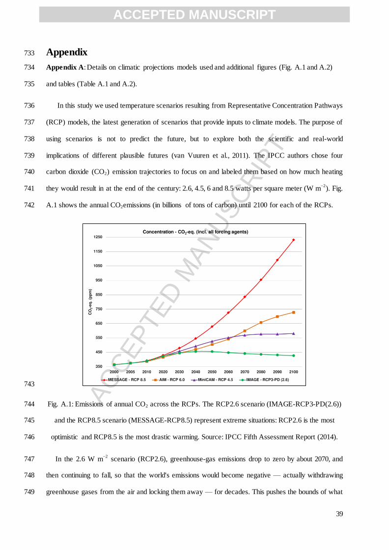
A.1 shows the annual CO2emissions (in billions of tons of carbon) until 2100 for each of the RCPs. 742

743

Fig. A.1: Emissions of annual CO2 across the RCPs. The RCP2.6 scenario (IMAGE-RCP3-PD(2.6)) 744

and the RCP8.5 scenario (MESSAGE-RCP8.5) represent extreme situations: RCP2.6 is the most 745

optimistic and RCP8.5 is the most drastic warming. Source: IPCC Fifth Assessment Report (2014). 746

In the 2.6 W m−2

scenario (RCP2.6), greenhouse-gas emissions drop to zero by about 2070, and 747

then continuing to fall, so that the world's emissions would become negative — actually withdrawing 748

greenhouse gases from the air and locking them away — for decades. This pushes the bounds of what 749

ACCEPTED MANUSCRIPT

ACC

EPTE

D M

ANU

SCR

IPT

40

is plausible through mitigation, some experts say. At the high end, in the 8.5 W m−2

scenario 750

(RCP8.5), CO2 levels would soar beyond 1,300 parts per million by the end of the century and 751

continue to rise rapidly (Table A.1). 752

Table A.1: Description of CO2 emissions scenarios used by IPCC authors (van Vuuren et al., 2011). 753

Scenario Description

RCP8.5 Rising radiative forcing pathway leading to 8.5 W m2 (~1370 ppm CO2 eq) by 2100.

RCP6 Stabilization without overshoot pathway to 6 W m

2 (~850 ppm CO2 eq) at stabilization

after 2100.

RCP4.5 Stabilization without overshoot pathway to 4.5 W m

2 (~650 ppm CO2 eq) at stabilization

after 2100.

RCP2.6 Peak in radiative forcing at ~3 W m

2(~490 ppm CO2 eq) before 2100 and then decline (the

selected pathway declines to 2.6 W m2 by 2100).

Atmospheric temperature data were obtained from the CERFACS modeling center. For each 754

scenario (RCP2.6 and RCP8.5) 14 models were available (http://cmip-755

pcmdi.llnl.gov/cmip5/availability.html; Table A.2). To know which model was the most comparable 756

to our historical temperature data in the Bay of Brest and the Bay of Saint Brieuc, we used the diagram 757

of taylor (Fig. A.2) in order to compare monthly air temperature since 1960 to nowadays in our bays 758

with monthly air temperature from the 14 models during the same period. Among the 14 models, the 759

CNRM-CM5 model was the best (Fig. A.2). 760

Table A.2: Description of the 14 models available for the study. 761

Modeling Center Model N° Institution

BCC BCC-CSM1.1 1 Beijing Climate Center

CCCma CanESM2 2 Canadian Centre for Climate Modelling and Analysis

NCAR CCSM4 3 National Center for Atmospheric Research

NSF-DOE-NCAR CESM1(CAM5) 4

National Science Foundation, Department of Energy, National Center for Atmospheric Research

CNRM-CERFACS

CNRM-CM5 5

Centre National de Recherches Météorologiques / Centre Européen de Recherche et Formation Avancées en Calcul Scientifique

LASG-IAP FGOALS-g2 6 LASG, Institute of Atmospheric Physics

NOAA GFDL GFDL-CM3 7 Geophysical Fluid Dynamics Laboratory

INPE HadGEM2-ES 8 Instituto Nacional de Pesquisas Espaciais

IPSL IPSL-CM5A-LR 9 Institut Pierre-Simon Laplace

IPSL-CM5A-MR 10

MPI-M MPI-ESM-LR 11 Max Planck Institute for Meteorology

ACCEPTED MANUSCRIPT

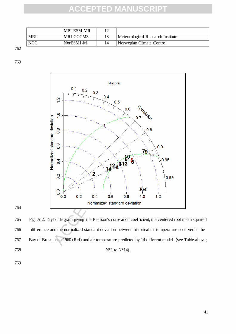
ACC

EPTE

D M

ANU

SCR

IPT

41

MPI-ESM-MR 12

MRI MRI-CGCM3 13 Meteorological Research Institute

NCC NorESM1-M 14 Norwegian Climate Centre

762

763

764

Fig. A.2: Taylor diagram giving the Pearson's correlation coefficient, the centered root mean squared 765

difference and the normalized standard deviation between historical air temperature observed in the 766

Bay of Brest since 1960 (Ref) and air temperature predicted by 14 different models (see Table above; 767

N°1 to N°14). 768

769

ACCEPTED MANUSCRIPT