CHAPTER . VI

A NEW METHODOLOGY AND SOFTWARE PACKAGE CREAM FOR IMPACT SUMMATION

6.1 INTRODUCTION

6.2 METHODOLOGICAL DETAILS OF CREAM

6.2.1 Problem smchm

6.2.2 Analysis

6.2.3 Graphical representation of the results

6.3 APPLICATION OF THE CREAM TO ROORKEE

6.3.1 Definition of base level

indicators

6.3.2 Weighting factors

6.3.3 Ideal and worst values

6.3.4 Analysis of the system states

6.3.5 Sensitivity analysis

6.3.6 Analysis of the development

policies

6.1 INTRODUCTION

An EIA is cansidered complete only after all the relevant variables, at least all the ones that have significant impacts, have been assessed, individually as well as collectively, to get a holistic perspective of the system under study. In the earlier chapters we have described studies on the nexus between the various variables of the system and the impact on if of individual variables, and vice-versa In this chapter we present a methodology that we have developed to understand the system CIS a whole. The methodology is based on network analysis. A software CREAM (Computer-aided Rapid Environmental impact Assessment and Management) has been devel- oped on the basis of this methodology. Typical print outs of cream are shown in Figure 6.1 (a-i). The methodology has been applied to generate and evaluate developmental scenarios for the city of Roorkee.

6.2 METHODOLOGICAL DETAILS OF CREAM

6.2.1 Problem structure

U Problem tree

a) Environment consists of myriad interconnected and interdependent aspects. Each of these can be characterized by some basic indicator. To analyse the whole system, basic indicators of each aspects of the environment need be studied and out of these the most relevant ones are to be selected to represent the system as

Figure 6.19 : Software package CREAM

Figure 6.1 h : Main menu of CREAM

Figure 6 . lc : Edit menu of the sofhvarr

Figure 6.Id : File reading in CREAM

Figure 6.le : A typical data entn

Figure 6.1f: Options available for evaluating a problem

Figure 6 . 1 ~ : A typical output of final scores of the system

Figure 6.lh : Report of detailed analysis

Figure h.li : Graphical representation of the results

holistically as practicable. We have called these indicators as basic indicators or Jirst-level variables.

b) These indicators may be grouped under broad categories based on the particular aspect ofthe environment they indicate: economic, sociocultural, etc. (Table 6.1). We have termed categorim as second-level varlables.

c) The second-level variables may be further grouped to fonn the third-level vml- ables, and so on. (Table 6.1)

d) Second -level variables, or further levels if any, are collectively termed as com- posite indicators.

ii) Ideal and worst value of variable$

basic indicator is to be assigned an iakal value and a worst value. These may be assigned on the basis of any of these criteria:

a) values that are indicated as 'ideal' by environmental standards (for example mo BOD is an ideal value for a river water according to water quality standards);

b) values that we know as ideal or more precisely 'best achievable' born past expe- rience or knowledge (for example yield of fish from a river or harvest of rice from a farm; the best achieved in the past may be set as 'ideal'); and

c) values we may want to be attained (example a population growth rate of z m or eradication of a disease).

iii) Weiahina the variable8

Each basic indicator is to k assigned a value which would show the extent of importance of the indicator. The weightage is to be assigned in such a way that the sum of all values in one group should total one. In order to determine these weightages either a Delphi may be conducted or w of standads can be made. Tbe same method applies to second, third, et al. levels of vari- ables (Table 6.2).

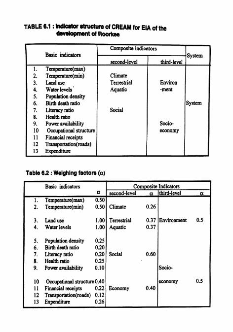
TABLE 6.1 : Indl#tor 8tfUCt~re of CREAM for EIA of ~ l e dwebpnmnt ot Roorkes

Table 6.2 : Welghlng factor8 (a)

- Basic indicators

1. T e m m m a x ) 2. Tempmlm(min) 3. Landuse 4. Water levels' 5. Populehon density 6. Birth death ratio 7. Literacyratio 8. Health ratio 9. Power availability 10 Occupational structure 1 1 Financial receipts 12 Transpoltation(r0ads) 13 Expenditure

Basic indicators a

1. Temp*.ahlre(max) 0.50 2. Temperature(min) 0.50

3. Land use 1.00 4. Water levels 1.00

5. Population density 0.25 6. Birth death ratio 0.20 7. Literacy ratio 0.20 8. Health ratio 0.25 9. Power availability 0.10

10 Occupational structure 0.40 11 Financial nccipts 0.22 12 Transpoltation(roads) 0.12 13 Expenditure 0.26

Composite indicators SY-

System

second-level

Climate Terrestrial Aquatic

Social

Composite Indicators

i

third-level

Environ - m a t

Socio- economy

second-level a

Climate 0.26

Terrestrial 0.37 Aquatic 0.37

Social 0.60

Economy 0.40

third-level a

Environment 0.5

Socio-

economy 0.5

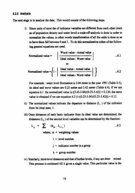
The next stage is to analyse the data. This would consist of the following steps.

i) Since units of most the of indicator variables are different from each other (such as of population density and water level) a trade-off analysis is done in order to normalize the values; in other words transformation of all the units is done so as to have them fall between 0 and 1. To do this normalization either of the follow- ing general equations are used.

Worst value -Actual value Normalid value =

Ideal values - Worst value I Ideal value - Actual value

Ideal values - Worst value

For example : water level fluctuation is 3.04 meter in the year 1991 (Table 6.5); its ideal and worst values are 0.25 meter and 3.42 meter (Table 6.4). If we use equation 6.1 the normalized value is l(3.42-3.04Y(0.25-3.42)1= 0.120; the same value is obtained if we use equation 6.2 (1-l(0.25-3.04)/(0.25-3.42)l) = 0.12.

ii) The normalid values indicate the departure or distance (L, ) of the indicator from its ideal state, 1.

iii) Once distances of each basic indicator from its ideal value are determined, the distances (L, ) of the second level variables can be determined by the function:

where, a = weighting values

i = level number

j = indicator number in a group

k = group number

iv) Similarly, third-level distances and that of further levels, if any are deter mined.

This process is continued till it gives a single value. This particular value is the

composite representation of the system as shown in Table 6.3.

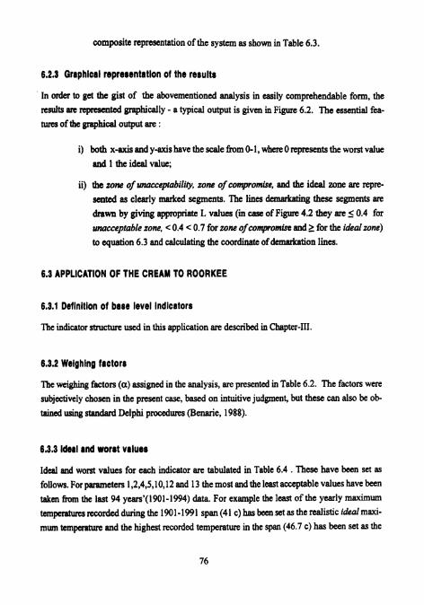
6.2.3 Graphlcal rrprrarntatlon of the results

In order to get the gist of the abovementioned analysis in easily comprehendable form, the results an rcpmmted graphically - a typical output is given in Figure 6.2. The essential fea- tures of the graphical output are :

i) both x-axis and y-axis have the scale from 0-1, where 0 represents the worst value and 1 the ideal value;

ii) the wne of unacceptability, wne of compromise, and the ideal zone are repre- sented as clearly marked segments. The lines dcmarkating these segments are

drawn by giving appropriate L values (in case of Figure 4.2 they an 5 0.4 for unacceptable zone, < 0.4 < 0.7 for zone of compromise and 2 for the ideal zone) to equation 6.3 and calculating the coordinate of demarkation lines.

6.3 APPLICATION OF THE CREAM TO ROORKEE

6.3.1 Deflnltion of base level Indicators

The indicator structure used in this application are described in Chapter-111.

6.3.2 Wrlghlng factors

The weighing factors (a) assigned in the analysis, are presented in Table 6.2. The factors were subjectively chosen in the present case, based on intuitive judgment, but these can also be ob- tained using standard Delphi procedures (Benarie, 1988).

6.3.3 l d u l and worrt valura

Ideal and worst values for each indicator are tabulated in Table 6.4 . These have been set as follows. For parameters 1,2,4,5,10,12 and 13 the most and the least acceptable values have been taken h m the last 94 yuus'(1901-1994) data. For example the least of the yearly maximum temperatures recorded during the 190 1 - 1991 span (4 1 c) has been set as the realistic ideal maxi- mum temperature and the highest recorded temperature in the span (46.7 c) has been set as the

TABLE 6.3 : Patbm of analysis at different level8 considered in CREAM

Whm, W : Wotst Value I : Ideal Value A : Actual Value , IV, : Importance Values at level 1,2,3, .... etc. L : Distances at levels 1,2,3 ,.... etc.

wi-A, L,, = 1 - - L , = ~ L , - N , L , ,=xL, .N, L d j E z LsN,

Ii- wi

1. Temperatm(max) 2. Temperature(min) 0.231

3. Land use 4. Water levels

0.405

5. Population density 0.951 6. Birth death ratio 0.1% 7. Literacy ratio 0.302 8. Health ratio 0.304 9. Power availability 0.781

10 Occupational structure 0.625 1 1 Financial receipts 0.742 12 Transportation(roads) 0.4 17 13 Expenditure 0.271

Social 0.502

Economy 0.534

Socio-

economy 0.5 14

Fipre 6 3 : Positions of rry~tem stria (of the city of Roorkee) if the cxiating trends persist

TABLE 0.4 : ldecrland wonrt values

Indicators

1 . Temperature(max) 2. Temperature(rnin) 3. Land use 4. Water levels 5. Population density 6. Birth death ratio 7. Literacy ratio 8. Health ratio 9. Power availability 10 Occupational structure I 1 Financial receipts 12 Transportation(roads) 13 Expenditure

Values Ideal

41.00 3.60 0.46 0.25 4480 1.00 1.00 2.00 1 .OO 0.28 28.76 267.90 9.80

Worst

46.70 1.00 1.00 3.42 14572 5.53 0.57 0.1 1 0.27 0.20 0.00 55.00 123.00

worst. For pammetcr 3 the lowest recorded builtup area ': total area ratio has been set as the ideal while the maximum possible value for the ratio (1) has been set as the worst.

For p m e t e r s 6,7 and 9 the best attainable state has been set as ideal while the worst recorded state has been taken as worst. For parameter 11 the worst possible situation of zero receipts has bem set as the worst frame of refmnce ; the best values a k e d so far has been set as the ideal.

6.3.4 Anaiysb of the system states

The values of these indicators were calculated from the data for Roorkee for the period 1961- 1994 (Table 6.5). The data was collected b m myriad sources and is given in Chapter-III. The indicator values for the years 2001,201 1 and 2021 were obtained by extrapolating the 1961 - 1994 data using regression analysis, performed with software package SMART-ALEC (Chap ter-V) assuming that the past trends would be persisting in future.

The results are summarised in Figure 6.2. The analysis reveals that the pattern of develop ment till 1961 was environmentally compatible. In subsequent years the stress due to develop ment began to unsettle the environment and the system state is passing through a zone ofcorn- promise from the 1960s. In each passing decade the system state is drifting farther and farther away from environmentally compatible zone and by 2001 it would cross the threshold ofzone of compromise and will enter the zone of unacceptnbility.

Figure 6.2 presents graphically how close or far the past system states, and the forecasts, are from the ideal state.

8.3.5 Sensitivity analysis

Sensitivity analysis was performed employing the data from Tables 6.5 and 6.6 by varying the weighing factors (Table 6.2). The findings in brief are:

i) at the level 111, the system state was more sensitive to environmentdmlogical than socio-economic factors;

ii) at the level I1 the system state was most sensitive to terrestrial and aquatic

indicators; and

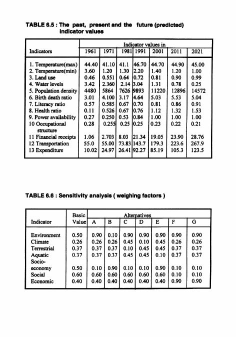
TABLE 6.5 : The past, present and the future (predicted) indicator values

TABLE 6.6 : Sensitivity analysis ( weighing factors )

Indicators

1. Temperature(max) 2. Temperature(min) 3. Land use 4. Water levels 5.Populationdensity 6. Birth death ratio 7. Literacy ratio 8. Health ratio 9. Power availability

Indicator values in

Indicator

Environment Climate Ternstrial Aquatic Socio- economy Social Economic

1961

44.40 3.60 0.46 3.42 4480 3.01 0.57 0.11 0.27 0.28 0.255 10 Occupational

structure 11 Financial receipts 1.06 2.703 12 Transportation 55.0 55.00 13 Expenditure 10.02 24.97

Basic Value

0.50 0.26 0.37 0.37

0.50 0.60 0.40

1971

41.10 1.20 0.551 2.360 5864 4.100 0.585 0.526 0.250

0.25 0.23 i::: 8.03 21.34 19.05 23.90 73.83 143.7 179.3 223.6 26.41 92.27 85.19 105.3

i:! 28.76 267.9 123.5

Alternatives

1981

41.1 1.30 0.64 2.14 7626 3.17 0.67 0.67 0.53

A

0.90 0.26 0.37 0.37

0.10 0.60 0.40

1991

46.70 2.20 0.72 3.04 9893 4.64 0.70 0.76 0.84

F

0.90 0.26 0.37 0.37

0.10 0.10 0.90

B

0.10 0.26 0.37 0.37

0.90 0.60 0.40

G

0.90 0.26 0.37 0.37

0.10 0.10 0.90

2001

44.70 1.40 0.81 1.31 11220 5.03 0.81 1.12 1.00

C

0.90 0.45 0.10 0.45

0.10 0.60 0.40

2011

44.90 1.20 0.90 0.78 12896 5.53 0.86 1.32

2021

45.00 1.00 0.99 0.25 14572 5.04 0.91 1.53

D

0.90 0.10 0.45 0.45

0.10 0.60 0.40

E

0.90 0.45 0.45 0.10

0.90 0.60 0.40

iii) at the base level , the indicators governing the system state most strongly were land-use pattern and water level.

6.3.6 Anrlyris of the development policier

These findings were wnveyed to the Municipal Council of the city of Rwrkee. They wnsid- md these f~ndings in the contcxt of their developmental priorities and availability of resources and zeroed on thne sets of desirable goals, or scenarios, presented as GI, G2 and G3 in Table

6.7. These scenarios wcre worked out by them towards realisation of the following alternatives.

0 Devekgmmt ootion G I

1. Increasing the Municipal area by 8 km with a mandatory 20% open area.

2. Introducing intermittent Water supply ( reduction by 7 M d a y ) i.e 200 lpcd in

stead of 368 lpcd per day.

3. Reduce Birth : death ratio as to become 4.00 by increasing awareness, through campaigns like family planning and by opening family welfare centres.

4. In- literacy by effectively running the evening schools and adult education centers.

5. Entqreneurship camps to promote self-employment.

1. A provision of minimum 20% of open area around buildings. Plantation of trees on either side of roads or in children parks,stadiums etc.

2. Reduce Birtkdeath ratio as to become 4.00 by increasing awareness, through campaigns like family planning and by opening family welfare centm.

3 Provision for more opportunities for development of self employment based in- dustries.

TABLE 6.7 : Modified values according to development options

Indicators

1. Tempc&m(max) 2. T e m m m i n ) 3. Land use 4. Water levels 5. Population density 6. Birth death ratio 7. Litcracy ratio 8. Hdth ratio 9. Power availability 10 Occupational

structure 1 1 Financial receipts 2 1.34 19.05 20.87 19.05 22.87 12 Tmsportation 143.7 179.3 215.1 179.3 215.1 13 Expenditure 92.27 85.19 119.1 140.6 147.6

Existing status (1991)

46.70 2.20 0.72 3.04 9893 4.64 0.70 0.76 0.84 0.25

Forecast for 2001 AD

44.70 1.40 0.81 1.31 1 1220 5.03 0.81 1.12 1.00 0.23 0.27 0.29 0.26

Scenario

G1

44.70 1.40 0.65 1.92 7453 4.01 0.98 1.12 1 .OO

G2

44.70 1.40 0.80 1.71 9697 4.01 0.90 1.12 1.00

G3

44.70 1.40 0.65 1.71 8976 5.03 0.81 1.34 1.00

u) Develooment o~t ion G9

1. Increasing the Municipal a m by 8 km . 2. Plantation of trees on either side of roads or in parts etc.

3. Increasing Medical Facilities and no. of dwtors in the hospitals.

4. Provision for more opporhnities for development of self employment based in- dustries.

For each development option appropriate indicator values and figures of monetary re- s o w ~ ~ ~ were introduced. They wished to know which of these has the potential of achieving the best system-state vis-a-vis environmental as well as economic criteria Accordingly the three scenarios were assessed with the aid of CREAM.

The following decision inputs emerge from the analysis:

i) the us it is trend is the least desirable; and

ii) GI is the best of the options whereas G2 and G3 show marginal improvement over the existing trend.

Graphically, the position of the four scenarios with respect to the ideal state is presented in Figure 6.3. The scenario GI is closest to the ideal and therefore the most desirable of the ones considered.

Figure 6 3 : The system 8trtea achievable in ZOO1 AD with development scenarios GI, G2 md G3.