Embed Size (px)
Citation preview

New Product Diffusion with Influentials and Imitators
Christophe Van den Bulte The Wharton School, University of Pennsylvania
Philadelphia, Pennsylvania 19104, U.S.A. [email protected]
Yogesh V. Joshi The Wharton School, University of Pennsylvania
Philadelphia, Pennsylvania 19104, U.S.A. [email protected]
July 2005
Acknowledgements We benefited from comments by David Bell, Albert Bemmaor, Xavier Drèze, Peter Fader, Donald Lehmann, Gary Lilien, Piero Manfredi, Paul Steffens, Stephen Tanny, Masataka Yamada, and audience members at the 2005 Marketing Science Conference. We also thank Peter Fader for providing the SoundScan CD sales data. Correspondence address: Christophe Van den Bulte, The Wharton School, University of Pennsylvania, 3730 Walnut Street, Philadelphia, PA 19104-6340. Tel: 215-898-6532; fax: 215-898-2534; e-mail: [email protected].
i

New Product Diffusion with Influentials and Imitators
Abstract
We model the diffusion of innovations in markets where the set of ultimate adopters consists of
two segments: influentials, who are more in touch with new developments and affect another
segment of pure imitators, whose own adoptions do not affect the influentials. This two-segment
structure is consistent with several theories in sociology and diffusion research as well as many
“viral” or “network” marketing strategies. There are four main results. (1) Diffusion in a mixture
of influentials and imitators can exhibit a dip or “chasm” between the early and later parts of the
diffusion curve. (2) The proportion of adoptions stemming from influentials need not decrease
monotonically but may start increasing again. (3) Erroneously specifying a mixed-influence
model to a mixture process where influentials act independently from each other can generate
systematic changes in the parameter values reported in earlier research. (4) Empirical analysis of
33 different data series indicates that the two-segment model fits better than the standard mixed-
influence, the Gamma/Shifted Gompertz, and the Weibull-Gamma models, especially in cases
where a two-segment structure is likely to exist. Also, the two-segment model fits marginally
better than the recent Karmeshu-Goswami mixed-influence model in which the coefficients of
innovation and imitation vary across potential adopters in a continuous fashion.
Key words: Diffusion of innovations; social contagion; social structure.
ii

1. Introduction
With the fragmentation of mass media, the deepening skepticism of consumers towards
advertising and marketing, and the decreasing ability of salespeople to reach business customers,
companies are under pressure to increase their marketing ROI through more astute targeting of
resources. Meanwhile, at a broader societal level, technologies like Minitel and the Internet have
boosted opportunities for information sharing among consumers, and a renewed appreciation has
emerged for how social identification and status considerations pervade consumption (e.g.,
Ehrenreich 1990; Maffesoli 1996; Schor 1998). In response to these developments, marketers are
rediscovering the importance of social contagion. This is especially so for new products which
only the most involved and knowledgeable customers may be aware of at first, and for new
products with considerable functional, financial, or social risk so mainstream customers are
likely to seek information from peers.
The newly deployed “viral” and “network” marketing strategies often share two key
assumptions: (1) some customers are more in touch with new developments, and (2) some (often
but not always the same) customers’ adoptions and opinions have a disproportionate influence—
direct or indirect—on others’ adoptions (e.g., Gladwell 2000; Moore 1995; Rosen 2000;
Slywotzky and Shapiro 1993). Targeting those influential prospects who are more in touch with
new developments and converting them into customers, the logic goes, allows marketers to
benefit from a social multiplier effect on their marketing efforts. The two assumptions are quite
reasonable, as they are consistent with several theories and a large body of empirical research
(e.g., Katz and Lazarsfeld 1955; Keller and Berry 2003; Rogers 2003), and the social multiplier
logic cannot be faulted either (e.g., Case et al. 1993; Valente et al. 2003). Yet, marketing science
provides little or no additional theoretical or descriptive insight on how new products diffuse in
1

such markets. The reason is that the great majority of marketing diffusion models assume
homogeneity rather than heterogeneity in the tendency to be in tune with new developments or
the tendency to influence (or be influenced by) others, and often assume homogeneity in both.
The present analysis addresses this gap between theory and emerging practice on the one hand,
and marketing diffusion models on the other. Specifically, we model the aggregate-level
diffusion path of a new product when the set of ultimate adopters is not homogenous but consists
of two segments: influentials who are more in touch with new developments and who affect
another segment of pure imitators whose own adoptions do not affect the influentials. We allow
for the presence or absence of contagion among influentials.
While many diffusion models incorporate the dual drivers of independent decision making
affected by being in touch with new developments and of imitation driven by others’ prior
adoptions, they do so under the assumption that all potential adopters are ex ante affected equally
by both factors. Taga and Isii (1959) in statistics, Mansfield (1961) and Williams (1972) in
economics, Coleman (1964) in sociology, and Bass (1969) and Massy, Montgomery and
Morrison (1970) in marketing, all advanced a model specifying the rate at which actors who have
not adopted yet do so at time t as h(t) = p + qF(t), where F(t) is the proportion of ultimate
adopters that has already adopted, parameter q captures social contagion, and parameter p
captures the time-invariant tendency to adopt early affected by consumer characteristics, the
innovation’s appeal, and efforts of change agents.1 Since the proportion that adopts at time t can
be written as f(t) = dF(t)/dt = h(t) [ 1 – F(t) ], one obtains:
f(t) = dF(t)/dt = [ p + qF(t) ] [ 1 – F(t) ] [1]
The solution of this differential equation can be written as:
1 Following the convention in marketing, we refer to the rate at which non-adopters turn into adopters as the hazard rate and denote it as h(t), even though the models we discuss are deterministic rather than probabilistic.
2

F(t) = [1 - e-g-(p+q)t] / [1 + (q/p) e-g-(p+q)t] [2]
where g acts as a location parameter fixing the curve on the time axis (e.g., Mansfield 1961).
When t = 0 corresponds to the actual launch time such that F(0) = 0, then g = 0 and equation (2)
reduces to the solution popular in marketing:
F(t) = [1 - e-(p+q)t] / [1 + (q/p) e-(p+q)t] [3]
The rate is influenced by both the intrinsic tendency to adopt (p) and social contagion (q) at all
times except at t = 0 when qF(0) = 0. To reflect this dual influence, Mahajan and Peterson (1985)
refer to the model as the mixed-influence model. Because the rate contains no contagion pressure
at t = 0, those adopting at that time are sometimes referred to as innovators and contrasted
against all others adopting later who are called imitators (e.g., Bass 1969). However, as several
researchers have noted over the years, this terminology can be used only ex post and the model
does not represent a diffusion process in an ex ante mixture of two segments, the first adopting
independently at a constant rate of p and the second segment driven only by social contagion and
adopting at rate qF(t) (e.g., Bemmaor 1994; Jeuland 1981; Lekvall and Wahlbin 1973; Manfredi
et al. 1998; Steffens and Murthy 1992; Tanny and Derzko 1988).
The objective of this study is, in the spirit of Bass (1969), Miller et al. (1993) and Moorthy
(1993), to mathematically formalize theoretical arguments and behavioral research findings and
to use this formalization to generate more refined theoretical insights on new product diffusion in
a population of influentials and imitators. This is important as marketing practitioners
increasingly deploy strategies assuming such a market structure and as marketing researchers
increasingly incorporate social structure into their diffusion investigations (e.g., Bronnenberg
and Mela 2004; Frenzen and Nakamoto 1993; Putsis et al. 1997; Van den Bulte and Lilien 2001).
3

Our results offer formalized insights into some current substantive and methodological
research questions. First, diffusion in a mixture of influentials and imitators can exhibit a dip or
“chasm” between the early and later parts of the diffusion curve. While this is a popular
contention (e.g., Moore 1991), our model shows that it need not be necessary for firms to change
their product to gain traction among later adopters and the adoption curve to swing up again.
Like Steffens and Murthy (1992) and Karmeshu and Goswami (2001) but unlike Goldenberg et
al. (2002), we obtain this result from a closed-form solution, and unlike those prior analyses, we
show that a dip can occur even when influentials act independently from each other. Second, the
proportion of adoptions stemming from influentials need not decrease monotonically but may
start increasing again. The management implication is that, while it may make sense to shift the
focus of one’s marketing efforts from influentials to imitators shortly after launch as shown by
Mahajan and Muller (1998) using a two-period model, one may want to revert one’s focus back
to influentials later in the process. Third, erroneously specifying a mixed-influence model to a
two-segment process can generate the systematic changes in the parameter values over time
reported in several studies. This analytical result is a specific formalization of Van den Bulte and
Lilien’s (1997) more general but qualitative argument that unaccounted heterogeneity in p or q
can generate changes in these parameters. Our result also complements Bemmaor and Lee’s
(2002) simulation analysis since we consider heterogeneity in a process where genuine contagion
exists rather than in a Gamma/Shifted Gompertz process without contagion.
We also perform an empirical analysis and assess the descriptive performance of the two-
segment model compared to that of the mixed-influence model and of three diffusion models
incorporating heterogeneity in the form of a continuous rather than a discrete mixture. Given the
difficulty of unambiguously identifying causal processes from aggregate diffusion data
4

(Bemmaor 1994; Hernes 1976; Lekvall and Wahlbin 1973; Lilien et al. 1981; Van den Bulte and
Stremersch 2004), the objective of this empirical analysis is not to conclusively demonstrate the
validity of any model. Rather, it is to assess whether the differences between the discrete mixture
and other models are sufficiently important to lead to differences in descriptive performance
when applied to data of interest to marketing researchers. The two-segment model fits better than
the mixed-influence, Gamma/Shifted Gompertz (Bemmaor 1994), and Weibull-Gamma models
(Hardie et al. 1998; Massy et al. 1970; Narayanan 1992), especially in cases where a two-
segment structure is likely (or even known) to exist, and fits slightly better than a recently
advanced mixed-influence model where p and q vary across potential adopters in a continuous
fashion (Karmeshu and Goswami 2001).
We proceed with first outlining our model setting, and within that context, discuss five
theories and frameworks that suggest the existence of ex ante influentials and imitators. Next, we
develop a macro-level model of innovation diffusion in such a setting. Subsequently, we discuss
how this model relates to the familiar mixed-influence model and to prior work on two-segment
models by Jeuland (1981), Tanny and Derzko (1988) and Steffens and Murthy (1992). Finally,
we report on the descriptive performance of the influential-imitator model compared to that of
the mixed-influence and continuous-mixture models.
2. Theories motivating a two-segment structure of influentials and imitators
The situation we model is the following. The set of eventual adopters has a constant size M
and consists of two a priori different types of actors, influentials and pure imitators. We use the
subscripts 1 and 2 to denote each type, and the subscript m to denote the entire mixture
population of adopters. We use θ to denote the proportion of type 1 actors in the population of
eventual adopters (0 ≤ θ ≤ 1), and F(t) to denote the cumulative penetration. Finally, w denotes
5

the relative importance that imitators attach to influentials’ versus other imitators’ behavior (0 ≤
w ≤ 1). Each type’s adoption behavior is then captured by the following hazard functions:
h1(t) = p1 + q1F1(t) [4]
h2(t) = q2[wF1(t) + (1-w)F2(t)] [5]
Note the double asymmetry in the influence process. First, type 1 may influence type 2, but the
reverse is not true. Since, ex ante, anyone of type 1 may influence anyone of type 2, we label the
former influentials, which is consistent with industry parlance (Keller and Berry 2003). Second,
unlike type 1, type 2 is driven only by contagion, so we label them imitators. Obviously, when θ
= 1 or q2 = 0, everyone falls into segment 1and the situation reduces to the mixed-influence
model. Also, when θ = 0, everyone falls into segment 2 and the situation reduces to the logistic
model. When imitators put equal weight on all prior adoptions regardless of origin, we have h2(t)
= q2Fm(t) = q2[θF1(t) + (1-θ)F2(t)], i.e., w = θ (as shown in Section 3).
The distinction between influentials and imitators is based on what drives their adoption
behavior, not on whether they adopt early or late. Hence, the distinction is different from that of
innovators vs. imitators in Bass (1969) and innovators vs. early adopters vs. early majority vs.
late majority vs. laggards in Rogers (2003). Conceptually, causal drivers and time of adoption
need not map one-to-one. Empirically, while those adopting early may act independently of
others, and those adopting late may be subject to contagion, this is not always so: many early
adoptions may be driven by contagion and the bulk of the late adoptions may stem from people
not subject to social contagion (e.g., Becker 1970; Coleman et al. 1966).
Several theories and conceptual models suggest such a two-segment structure, though there is
some disagreement on whether q1 may be larger than zero. We first describe sociological
arguments focusing on social character, social status, and social norms. Then, we turn to the two-
6

step flow hypothesis that focuses on interest in new developments, and finally to the chasm idea
that focuses on enthusiasm for innovations versus risk aversion.
2.1. Social character
In his classic treatise on the changing nature of modern society, Riesman (1950)
distinguished three types of social character: autonomous, inner-directed, and other-directed. The
first two have in common the presence of clear-cut internalized goals, but differ as to whether
these are consciously chosen (autonomous) or inculcated during youth by elders (inner-directed).
Other-directed actors, in contrast, use their peers as their source of direction. The typology is in
essence about conformity stemming from the need for approval and direction from others.
Riesman worked on a broad social and cultural canvas and his typology is best used to refer to
patterns of behavior found in a variety of specific contexts rather than to types of persons or
personalities. Yet, his concepts have direct relevance for consumer behavior (e.g., Riesman
1950; Schor 1998). Some actors in some situations will exhibit autonomous or inner-directed
adoption behavior independent from their peers (hence q1 = 0), while others will exhibit other-
directed behavior driven by social contagion from peers. Riesman did not narrowly specify who
these peers are, and allowed them to be all of society (so w = θ being possible).
2.2. Status competition and maintenance
People buy and use products not only for functional purposes but also to construct a social
identity, and to confirm the existence and support the reproduction of social status differences
(Bourdieu 1984). A long-held idea in diffusion theory is that people seek to emulate the
consumption behavior of their superiors and aspiration groups (e.g., Simmel 1971) and also
quickly pick up innovations adopted by others of similar status if they fear that such adoptions
might undo the present status ordering (Burt 1987). In short, actors tend to imitate the adoptions
7

of those of higher and similar social status.
Assuming one can divide the population in a high-status and a low-status group, status
considerations suggest that both groups may exhibit contagion. Higher-status actors may imitate
each other out of fear of falling behind (q1 ≥ 0), and lower-status actors will imitate to catch up.
Whose adoptions the imitators act upon is not clear a priori. One might argue that the only
adoptions that matter are those by the high-status influentials to which they want to move closer
(w → 1). However, most authors follow Simmel and posit a finer-grained hierarchy with
multiple strata (approximated imperfectly by a dichotomy) and a cascading pattern through the
population where all prior adoptions contribute equally to social contagion (w = θ). Finally, to
the extent that status is maintained by adhering to social norms enforced among one’s direct
peers of similar position, imitators should care mostly about fellow imitators (w → 0).
2.3. Middle-status conformity
Like theories of status competition and maintenance, middle-status conformity theory is
about one’s proper place in society. The main claim is that the relationship between status and
conformity to norms—and hence susceptibility to social contagion—is an inverted U (e.g.,
Homans 1961; Philips and Zuckerman 2001). Since high-status actors feel confident in their
social acceptance, they feel comfortable to deviate from conventional behavior and adopt
appealing innovations independently from others. Low-status actors feel free to deviate from
accepted practice and adopt innovations independently as well because they feel that this can not
hurt their already low status. Middle-status actors, in contrast, feel insecure and strive to
demonstrate their legitimacy by engaging in new practices only after they have been socially
validated. So, middle-status conformity theory is consistent with the presence of two kinds of
8

actors, one adopting as a function of the innovation’s appeal irrespective of others’ actions (q1 =
0), and one adopting as a function of the legitimation stemming from prior adoptions.
The theory does not specify whose adoptions are being imitated (w). Conformity pressures
allow for both selective “status-based” imitation and non-selective “frequency-based” imitation
(Haunschild and Miner 1997). Adoptions by high-status actors might legitimate the innovation in
the eyes of the middle-status actors disproportionately, in which case the relation of w to θ is
unclear as the latter captures both high and low status. Conversely, imitators may care only about
social acceptability among their middle-status peers, and hence care only about the latter’s
adoptions (w = 0). Finally, applications of neo-institutional theory to innovation adoption tend to
posit that the legitimacy of an innovation is affected by the overall penetration rate (w = θ).
Note, higher status is often associated with higher economic resources and hence a higher
ability to adopt innovations. This leads to the interesting prediction that only the adoptions at an
intermediate stage of the overall diffusion process (made by middle-status actors) exhibit
contagion (e.g., Cancian 1979), because the earliest adoptions will come from high-status actors
and the latest from low-status actors, none of which are subject to contagion.
2.4. Two-step flow
The two-step flow hypothesis, originally proposed to explain unexpectedly weak mass media
effects in presidential elections, posits that “ideas often flow from radio and print to the opinion
leaders and from them to the less active sections of the population” (Lazarsfeld et al. 1944, p.
151; emphasis in original). So, in its original and starkest version, the two-step flow hypothesis
posits two groups, one being affected only by mass media and the other being affected only by
social contagion. What distinguishes the two groups is the level of interest in the subject matter
and alertness to new developments rather than exposure to mass communications (Lazarsfeld et
9

al. 1944). Later studies in marketing have corroborated a strong relationship between opinion
leadership and product interest and involvement (e.g., Coulter et al. 2002; Myers and Robertson
1972). Note, the two-step flow hypothesis does not impose that an opinion leader in one sphere
(politics, fashion, computer games, etc.) also be a leader in another sphere, and several studies
indeed document only moderate to little overlap in leadership across product categories (e.g.,
Katz and Lazarsfeld 1955; Merton 1949; Myers and Robertson 1972; Silk 1966). So, the relative
size of the segments (θ) may vary across innovations. While early studies focused on information
flows from opinion leaders to less active members of the population, subsequent research has
documented extensive information exchange among opinion leaders (e.g., Coulter et al. 2002;
Katz and Lazarsfeld 1955). This would be consistent with q1 > 0.
The two-step flow hypothesis emphasizes the flow of information. The contagion mechanism
is one of information transfer increasing awareness of the product’s existence and decreasing its
perceived risk, not of normative legitimation or status competition. Of the five theories we
consider, this is perhaps the most familiar to marketers and the most flexible. For low-risk
innovations, for instance, the fraction of pure imitators in need of guidance can be quite small,
and θ quite large. Who is being imitated is not clearly specified, and w may range from 0 to 1.
The two-step flow idea emphasizes that mass media influence on the less-active segment
operates through opinion leaders who are the only ones to take an active interest in information
available in the media. It does so without constraining the social influence exerted on the less-
active segment to come only from opinion leaders, and allows for a cascading or rolling pattern
through the population where all prior adoptions contribute to social contagion (e.g., Katz 1957;
Merton 1949). This suggests w ≈ θ. However, it is quite possible that opinion leaders are more
influential, suggesting that—in the extreme case—they may be the only ones being imitated (w =
10

1). Conversely, it is also quite possible that imitators consider fellow imitators to be more
representative and hence valuable as information sources, suggesting low values of w.
2.5. High-technology adoption chasm
In Moore’s (1991) chasm framework for technology products, the so-called early market
consists of “technology enthusiasts” and “visionaries” who are quick to appreciate the nature and
benefits of the innovation, whereas the “mainstream” market consists of more risk-averse
decision makers and firms who fear being stuck with a technology that is not user friendly,
poorly supported, or at risk of losing a standards war. Whereas the mainstream market can be
represented as responding only to the size of the installed base, i.e., prior adoptions (Mahajan
and Muller 1998), Moore is unclear about the process among “technology enthusiasts” and
“visionaries”. Whereas his textual discussions suggest that they act independently (q1 = 0), his
stylized graph of the bell-shaped adoption curve with a chasm is mathematically inconsistent
with a constant-hazard process in the early stages of diffusion and requires q1 > 0.
Moore does not clearly specify whose adoptions are being imitated (w). On the one hand, one
might argue that the legitimacy of a new technology is affected by the penetration rate in the
overall population, i.e., the total installed base regardless of who adopted (w = θ). On the other
hand, Moore emphasizes that product versions appealing to technology enthusiasts and
visionaries need not appeal to the mainstream market, which implies that mainstream customers
discount adoptions by technology enthusiasts and visionaries and care only about adoptions by
other mainstream customers (w = 0).2
2 Moore himself is far from clear on the issue when discussing the relationship between “visionaries” in the early market and “pragmatists,” i.e., the early adopters among the members of the mainstream market. At one point, he admonishes the reader to “do whatever it takes to make [visionaries] satisfied customers so that they can serve as good references for the pragmatists” but on the very next page he writes that “pragmatists think visionaries are dangerous. As a result, visionaries, with their highly innovative … projects do not make good references for pragmatists” (Moore 1995, pp. 18-19).
11

2.6. Conclusion
At least five different theoretical frameworks imply modeling innovation diffusion using a
two-segment structure consisting of influentials and imitators (Table 1). Two theories suggest
that influentials adopt independently, implying q1 = 0, but the other three suggest that influentials
may exhibit contagion amongst themselves.3 The theories vary in their causal mechanisms and,
consequently, in what kind of actors belongs to each segment and who the imitators imitate (w).
Table 1: Theoretical frameworks suggesting an influential-imitator mixture
Framework Influentials Imitators Reason to imitate Who gets imitated a
Social character Autonomous and inner-directed; q1 = 0
Other-directed Looking for approval and direction
- Not specified, possibly all adopters (w = θ)
Status competition and maintenance
High status; q1 ≥ 0 Low status Gaining or maintaining status
- All adopters (w = θ) - Only influentials (w = 1) - Only imitators (w = 0)
Middle-status conformity
High and low status; q1 = 0
Middle status Conforming to social norms
- All adopters (w = θ) - Only influentials with high status - Only imitators (w = 0)
Two-step flow Active and involved (opinion leaders); q1 ≥ 0
Not active or involved
Transferring information
- All adopters (w = θ) - Only influentials (w = 1) - Only imitators (w = 0
Technology chasm Technology enthusiasts and visionaries; q1 ≥ 0
Mainstream customers
Reducing risk - All adopters (w = θ) - Only imitators (w = 0)
a Parameter w denotes how much the social contagion affecting the imitators stems from the influentials (w) rather than fellow imitators (1-w). Parameter θ is the fraction of ultimate adopters belonging to segment 1 (influentials).
The theories also suggest that the relative size of the segments (θ) can vary from innovation
to innovation. It may be quite low for very non-mainstream products that only a very small
pocket of “bleeding edge” customers find attractive but that in spite of the latter’s enthusiasm
take a long time to diffuse, resulting in an adoption curve with a long left tail. Conversely, for
products with low functional or financial risk and with little implications for social status, like
3 Independent decision making among influentials is also consistent with Midgley and Dowling (1978) who define innovativeness as “the degree to which an individual makes innovation decisions independently of the communicated experience of others” (p. 235). So our distinction between independent influentials (with q1 = 0) and imitators is the same as their dichotomy between “innate innovators” and “innate noninnovators” (p. 237).
12

marginally novel drugs or CDs and movies with already famous performers, most adopters may
feel little need for information or legitimation from peers. This implies a high θ, a low q1, and an
exponential-like diffusion process (e.g., Moe and Fader 2001; Van den Bulte and Lilien 2001). A
high θ is also expected when the large majority of adopters behave according to the mixed-
influence model, with consumer appliances being a likely candidate.
3. Two-segment mixture models
We seek closed-form solutions in the time domain for an innovation’s diffusion path when
the set of eventual adopters, which has a constant size M, consists of two a priori different types
of actors adopting according to equations (4) and (5). The overall cumulative penetration is
simply the average of both types’ cumulative penetration weighted by their constant population
weights (e.g., Cox 1959):
Fm(t) = θ F1(t) + (1−θ) F2(t) [6] Similarly, the fraction of the population adopting at time t is:
fm(t) = θ f1(t) + (1−θ) f2(t) [7] In contrast, the population hazard function is not an average of the two hazards weighted by each
segment’s constant population weights, but is given by:
hm(t) = fm(t) / [1−Fm(t)]
= [ θ f1(t) + (1−θ) f2(t) ] / [1−Fm(t)]
= π(t) h1(t) + [1−π(t)] h2(t) [8]
where fi(t) = hi(t) [1−Fi(t)] and π(t) is the proportion of actors not having adopted yet at time t
that belong to type 1:
π(t) = θ )(1)(1 1
tFtF
m−−
[9]
13

Finally, the proportion of adoptions taking place at time t that is made by actors of type 1 is:
φ(t) = θ f1(t) / fm(t) [10]
3.1. Influential-imitator mixture model (IIM), with q1 > 0
Having defined the key functions, and having made the behavioral assumptions in the hazard
functions (eqs. 4 and 5), we now develop the influential-imitator mixture model (IIM). The
process among the influentials is the well-known mixed-influence model. When F1(0) = 0, the
cumulative penetration function and instantaneous adoption function for influentials are:
)1/()1()( )()(1 11
1
111 tqppqtqp eetF +−+− +−= [11]
2)()(211 )1/())1(()( 11
1
111
1
1 tqppqtqp
pq eeptf +−+− ++= [12]
The diffusion path among imitators, in contrast, does not follow any standard diffusion model, as
it is driven by the prior adoptions of both influentials and other imitators. As shown in Appendix
A1, when F2(0) = 0, the cumulative penetration function for imitators in IIM is:
))1()1(()()1(
)1(1)(
211111
112
12
11
)11(112 HwqwpwqeHwq
wqwptF
qwq
tqp
qpeqptq −−−−+−
−−+=
++ +−
, where [13]
);1;,1( )11(11
1
11
2
1
2
1
2121 tqpeqp
pqp
wqq
wqFH +−++−+= , );1;,1(
11
1
11
2
1
2
1
2122 qp
pqp
wqq
wqFH++
−+= , and
2F1(1,b;c;k) is the Gaussian hypergeometric function:
2F1(1,b;c;k) = ∑∞
= +ΓΓΓ+Γ
0 )()()()(
n
nkncbcnb [14]
This hypergeometric series is convergent for arbitrary b, c if |k| < 1; and for k = ±1 if c > 1 + b.
This implies that the closed-form solution in equation (13) is well-defined as long as q1 > 0.4
Once F1(t) and F2(t) are known, one can obtain the instantaneous adoption function f2(t) by 4 While the Gaussian hypergeometric functions 2F1(1,b;c;k) can be simplified to incomplete beta functions, we do not perform this simplification as it requires the overly restrictive condition that p1w/(1-w) > q1.
14

substituting equations (11) and (13) into:
f2(t) = q2 [wF1(t) + (1-w) F2(t)] [1- F2(t)] [15]
With solutions for F1(t), f1(t), F2(t) and f2(t) available, one can enter those into equations (6)
through (10) to obtain closed-form solutions for the population-level functions.5 In Figure 1, we
plot the function fm(t) and its two components θf1(t) and (1-θ)f2(t) for four sets of parameter
values chosen to illustrate various types of diffusion behavior possible in this model:
Case (a): p1 = 0.05; q1 = 0.1; q2 = 0.2; θ = 0.15; w = 0.20;
Case (b): p1 = 0.01; q1 = 0.5; q2 = 0.2; θ = 0.15; w = 0.01;
Case (c): p1 = 0.05; q1 = 0.5; q2 = 0.2; θ = 0.30; w = 0.30;
Case (d): p1 = 0.01; q1 = 0.1; q2 = 0.2; θ = 0.15; w = 0.001.
Diffusion process (a) exhibits a bell-shaped adoption curve fm(t) that is unimodal and close to
symmetric around its peak. This is the pattern commonly associated with mixed-influence model.
Diffusion process (b) is bimodal and exhibits a marked dip because adoptions by influentials are
already well past their peak by the time the imitators start adoption in numbers (the delay being
caused by the low w value). This is the much-debated “chasm” pattern. Diffusion processes (c)
and (d), finally, are again unimodal but exhibit a clear skew to the right or left, which the mixed-
influence cannot account for very well (e.g., Bemmaor and Lee 2002).6 Note that in all four
cases, f1(t) reaches zero before f2(t) does, so the commonly expected association between being
5 Even though our closed-form solution for F2(t) in the IIM looks quite different from the solution presented by Steffens and Murthy (1992), theirs is actually nested in ours. After imposing the constraint w = θ, reparameterizing the Steffens-Murthy solution in terms of m, θ, p1, q1, and q2, correcting for a (most likely typographic) error in their solution, and performing additional derivations, one can show that our closed-form solution for F2(t) in the IIM, and hence Fm(t), is identical to theirs. One difference, though, is that their solution requires q1 > q2θ (or q1 > q2w) for a series expansion term in their solution to converge, whereas the solution in eq. (13) only requires q1 > 0. 6 All four patterns for the total number of adoptions shown in Figure 1 have been documented in prior research. Pattern (a) is probably the most commonly reported in the marketing literature. Steffens and Murthy (1992) and Karmeshu and Goswami (2001) report data series exhibiting the bimodal pattern (b). Dixon (1980) reports the presence of long right tails, i.e., pattern (c), in many of the data he analyzed. Van den Bulte and Lilien (1997) report several data series exhibiting long left tails, i.e., pattern (d).
15

an imitator and being a late adopter holds. Also note that, as one would intuit, low values of w
cause the diffusion among imitators to be delayed and f2(t) to shift to the right. We now turn to
the case where q1 = 0, and study it in some more detail using the functions hm(t), π(t), and φ(t).
Figure 1: Adoption functions for four IIM diffusion processes
3.2. Pure-type mixture model (PTM), with q1 = 0
When influentials adopt independently and q1 = 0, the situation is that of a pure-type mixture
(PTM) of pure independents and pure imitators. The process among the independents is the well-
known constant-hazard exponential process. When F1(0) = 0, we have:
F1(t) = 1 – e-p1t [16]
f1(t) = p1 e-p1t [17]
As shown in Appendix A2, when F2(0) = 0, the cumulative penetration function for imitators in
the PTM is:
16

F2(t) = )exp()),(),(())(1(
)exp(1
1
2
1
2
1
21
1
2
1
2
1
2
1
2
1
1
2
1
2
2
wwweww
wetq
pq
pq
pqtp
pq
pq
pq
pq
tppq
pq
−−Γ−Γ−
−−+
−−
−
[18]
where Γ(η,k) is the “upper” incomplete gamma function:
Γ(η, k) = dvev v
k
−∞ −∫ 1η
The instantaneous adoption function f2(t) is obtained by substituting equations (16) and (18)
into (15). With solutions for F1(t), f1(t), F2(t) and f2(t) available, one can enter those into
equations (6) through (10) to obtain closed-form solutions for the population-level functions. In
Figure 2, we plot the functions fm(t), hm(t), π(t), and φ(t) for three sets of parameter values chosen
to illustrate various types of diffusion behavior possible in this model7:
Case (a): p1 = .15, q2 = .50, θ = .25, w = .25;
Case (b): p1 = .25, q2 = .40, θ = .15, w = .01;
Case (c): p1 = .15, q2 = .65, θ = .60, w = .05.
Diffusion process (a) exhibits the common unimodal, symmetric-around-the-peak adoption
curve fm(t) well captured by the mixed-influence model. More interesting is that the hazard
function is not monotonic as in the mixed-influence model. Rather, it is roughly bell-shaped and
seems to converge to a value in between the minimum and the maximum. Here is why. The very
earliest adopters consist of independents and the population hazard equals θp1 = .0375 at first. As
more and more imitators adopt with hazard q2Fm(t), the population hazard increases. Once
q2Fm(t) > p1, which can happen quickly when q2 is markedly larger than p1, the set of imitators
not having adopted yet will start depleting faster than the set of independents not having adopted
7 Of the three shapes of adoption curve in Figure 2, pattern (a) is probably the most commonly reported in the diffusion literature. The other two shapes have not been documented as extensively, but do occur in previously analyzed data. For instance, the sales curve of several music CDs studied by Moe and Fader (2001) exhibit pattern (b) or (c), and the classic Medical Innovation data analyzed by Coleman et al. (1966) also exhibit pattern (c).
17

Figure 2: Plots of functions characterizing three PTM diffusion processes
(a) (b) (c) p1=.15, q2=.5, θ=.25, w=.25 p1=.25, q2=.4, θ=.15, w=.01 p1=.15, q2=.65, θ=.6, w=.05
18

yet. As a result, the laggards remaining to adopt consist increasingly of independents—as
indicated by the function π(t) reaching a minimum around t = 5 and then increasing to 1—and
the population hazard converges back to an asymptote of p1 = .15. This pattern of relative speed
of depletion also explains the non-monotonic pattern in φ(t), the proportion of adoptions taking
place at time t stemming from independents. Note that in this diffusion process, independents
make up the bulk not only of the early adopters, but also of the very late adopters. Importantly,
the point at which φ(t) starts increasing and independents start gaining rather than losing
importance (t = 7.3) occurs when the process is still far from complete and the remaining market
potential is still quite sizable (37 % since Fm(t) = .63 at t = 7.3).
Diffusion process (b) differs in several respects from process (a). First, the adoption curve f(t)
does not have a smooth bell shape but exhibits a clear dip early on. This is easily explained. The
independents adopt rapidly because p1 = .25 is rather high. However, imitators’ reaction to those
independent adoptions is very muted because they imitate mostly fellow imitators (w = .01). As a
result, the adoptions by independents show an exponential decline which is not immediately
compensated by the imitators’ slowly developing adoptions, resulting in an early dip in the
population curve. Note that independents account for the bulk of the adoptions only early in the
diffusion process, as φ(t) declines steeply to close to zero. So, while the adoption curve does not
fit the standard model, we do have the commonly expected association between being an imitator
and being a late adopter.
Diffusion process (c) is mostly an exponential process commonly observed for fast moving
consumer goods, CDs and films, but with a marked boost after the early periods. What is
happening is that most adopters are independents (θ = 60%), so the majority of adoptions follow
an exponential decline. However, there is also a sizable segment of imitators that are very
19

sensitive to social contagion (q2 = .65), but mostly from fellow imitators rather than
independents (w = .05). As a result, the imitators are slow to adopt at first, but once the snowball
starts rolling, tend to adopt in a very short time. This is reflected in the shape of φ(t): the
proportion of adoptions accounted for by independents tends to be close to 100%, except for a
relatively narrow time window during which it first declines and then increases again. The
contrast between process (a) and (c) is informative: They have similar p1 and q2 values, and the
composition of both adopters φ(t) and remaining non-adopters π(t) tend to evolve similarly, as do
their respective population hazard functions h(t). Yet, because of the different segment sizes θ
and contagion weights w in the two processes, the resulting adoption curves are quite different.
3.3. Some special cases of theoretical interest
Our review of prior theories and frameworks indicates that three cases of the IIM and PTM
are of special theoretical interest. The first is where imitators imitate only influentials (w = 1)
such that h2(t) = q2F1(t). The second is where imitators imitate only other imitators (w = 0) such
that h2(t) = q2F2(t). The third is where imitators randomly mix with both independents and
imitators such that w = θ and h2(t) = q2Fm(t). In the first and third case, F2(t) and f2(t) are easily
derived by imposing w = 1 and w = θ , respectively, in equations (13), (15) and (18). In the
second case, the process among imitators is only a function of prior adoptions by other imitators
and is simply the well-known logistic process.8 In all three special cases, the population-level
functions Fm(t), fm(t), hm(t), π(t), and φ(t) are readily obtained once F2(t) is known.
8 Note, when w = 0 or θ = 0, the process among imitators cannot get started within the model. As is well known, the closed-form solution for the logistic requires that F2(0) > 0. Hence, while the cases with w = 0 or θ = 0 are conceptually nested within IIM or PTM, their closed-form solutions are not as they make different assumptions about the initial conditions.
20

4. Relation to prior diffusion models
4.1. Mixed-influence model vs. pure-type mixture model
As the closed-form solutions and the plots in Figure 2 indicate, the mixed-influence model
(MIM) does not capture diffusion processes in a discrete mixture of pure independents and pure
imitators, regardless of the relative contagion influence of adoptions by independents vs.
imitators. The only two exceptions to this are the case where p1 = 0 or θ = 0 and both models
collapse to the logistic model, and the case where q2 = 0 or θ = 1 and both models collapse to the
exponential model.
Our analysis allows one to assess more rigorously the argument (e.g., Mahajan et al. 1993)
that rewriting the standard differential equation for the mixed influence model (eq. 1) into:
f(t) = p [ 1 - F(t) ] + qF(t) [ 1 - F(t) ] [19]
allows one to interpret the term p [ 1 - F(t) ] as the number adoptions made by people adopting
with hazard p and the term qF(t) [ 1 - F(t) ] as the number of adoptions made by people adopting
with hazard qF(t). While the manipulation of the equation is evidently correct, the interpretation
is not. The main reason is that, in each term, the fraction of actors not having adopted yet, 1-F(t),
refers to the total population, rather than to the fractions in each of the segments, 1-F1(t) and 1-
F2(t). In addition, the sizes of each segment are ignored. The correct expression for a mixture, is:
fm(t) = θ f1(t) + (1−θ) f2(t)
= θ h1(t) [1−F1(t)] + (1−θ) h2(t) [1−F2(t)]
= θ p1 [ 1 - F1(t) ] + (1-θ) q2[wF1(t) + (1-w) F2(t)] [ 1 - F2(t) ] [20]
When imitators randomly mix with independents and imitators and are equally affected by both,
then w = θ and the equation simplifies to:
fm(t) = θ p1 [ 1 - F1(t) ] + (1-θ) q2Fm(t) [ 1 - F2(t) ] [21]
21

Even if p = θp1, q = (1-θ)q2, and one omits the m-subscript from the population-level fm(t) and
Fm(t), the mixture equation (21) is different from the mixed-influence equation (19).
Within a homogeneous population with mixed influence, one can only interpret the relative
size of the two terms p[1-F(t)] and qF(t)[1-F(t)] as reflecting the relative influence of time-
invariant elements (p) versus social contagion (qF(t)) on the adoptions at time t, keeping in mind
that each and every adoption is influenced by both p and qF(t) for any t > 0. For instance, the
ratio p/(p+qF(t)) can be used as a measure of the relative strength of time-invariant elements at
time t (Lekvall and Wahlbin 1973), as can the decomposition presented by Daley (1967) and
Mahajan, Muller and Srivastava (1990), but neither can be interpreted as the fraction of all
adoptions at time t stemming from pure-type actors adopting a priori with hazard p.
Another common belief about the mixed-influence model that is inconsistent with its
mathematical structure is that “the importance of innovators will be greater at first but will
diminish monotonically with time,” where innovators are defined as those who “are not
influenced in the timing of their initial purchase by the number of people who have already
bought the product” (Bass 1969, p. 217). In a homogenous population where everyone behaves
according to the hazard rate p + qF(t), the only actors with hazard p are those adopting at t = 0
when F(0) = 0. Anyone adopting afterwards is influenced by prior adoptions. Hence, in the
mixed-influence model, the proportion of adoptions occurring at time t that are unaffected by
social contagion follows a step function with value 1 at t = 0 and value 0 for any t > 0.
Conversely, in a true discrete mixture, the proportion of independents adopting with a constant
hazard, i.e., function φ(t), need not diminish monotonically over time, as shown in Figure 2.
22

4.2. Consequence of imposing a mixed-influence structure on a pure-type mixture process
From comparing equations (19) and (21) one may get the impression that a diffusion process
in a discrete mixture with h1(t) = p1 and h2(t) = q2Fm(t) could be approximated quite well by a
mixed-influence model with h(t) = p + qF(t), even if they are not identical. However, the
adoption functions fm(t) and hazard functions hm(t) suggest some potentially important
deviations. More insight comes from re-writing the expression for fm(t) in eq. (21) into a form
similar to that for f(t) in the mixed-influenced model (following Manfredi et al. 1998):
fm(t) = θ p1 [ 1 - F1(t) ] + (1- θ) q2Fm(t) [ 1 - F2(t) ]
= [ θ p1 )(1)(1 1
tFtF
m−− + (1- θ) q2Fm(t)
)(1)(1 2
tFtF
m−− ] [ 1 - Fm(t) ]
= [ p(t) + q(t) Fm(t) ] [ 1 - Fm(t) ] [22]
where
p(t) = θ )(1)(1 1
tFtF
m−− p1 = π(t) p1 [23]
q(t) = (1-θ) )(1)(1 2
tFtF
m−− q2 = [1−π(t)] q2 [24]
Deleting the m subscript from equation (22) to reflect one’s ignoring that the population consists
of a mixture results in:
f(t) = [ p(t) + q(t) F(t) ] [ 1 - F(t) ] [25]
So, one is able to re-write the pure-type mixture model with w = θ into an expression akin to the
mixed-influence model, but with both hazard rate parameters varying systematically over time.
More specifically, p(t) changes in exactly the same way as π(t), the proportion of actors not
having adopted yet by time t that belong to the segment of independents. At t = 0, π(t) = θ and
p(t) = θp1. Since at the very beginning adoption tends to be more prevalent among independents
23

than among imitators, the number of independents who have not adopted yet gets depleted faster
than the number of imitators who have not. Consequently, π(t) and p(t) decline at first. However,
when q2 >> p1, the relative speed of adoption between the two segments quickly reverses and the
set of actors who have not adopted yet tends to become increasingly dominated by independents.
As a result, π(t) and p(t) increase over most of the time window. The reverse pattern takes place
for q(t) = [1−π(t)] q2. It starts at (1-θ)q2, increases for a very short period, but starts decreasing
very soon. Note, when θ ≈ 0 or θ ≈ 1, then π(t) will not vary much and neither will p(t) or q(t).
In short, specifying a mixed-influence model with h(t) = p + qF(t) when the true data
generating process is that of a discrete mixture with h1(t) = p1 and h2(t) = q2Fm(t) where q2 >> p1
will yield increasing values of p and decreasing values of q (except for the first very few
periods). This is consistent with the pattern in mixed-influence model estimates described in
prior research. Though Van den Bulte and Lilien (1997) focused their analysis on ill-
conditioning in the absence of model misspecification, they recognized that unobserved
heterogeneity in p and q forms an alternative explanation for the systematic changes they
observed in empirical applications. Our results formalize their argument for the case of two
segments where one segment has p = 0 and the other has q = 0.
4.3. Relation to other two-segment models
Figure 3 shows how our models relate to a few other models, including two earlier two-
segment models. Tanny and Derzko (1988) used a discrete mixture with h1(t) = p1 and h2(t) = p2
+ q2Fm(t). Steffens and Murthy (1992) used a discrete mixture with h1(t) = p1 + q1F1(t) and h2(t)
= q2Fm(t). So, as shown in Figure 3, both these models conceptually nest both the mixed-
influence model and PTM3 with w = θ. The diagram also shows that, like the mixed-influence
model, the pure-type mixture models have both the exponential and logistic models nested in
24
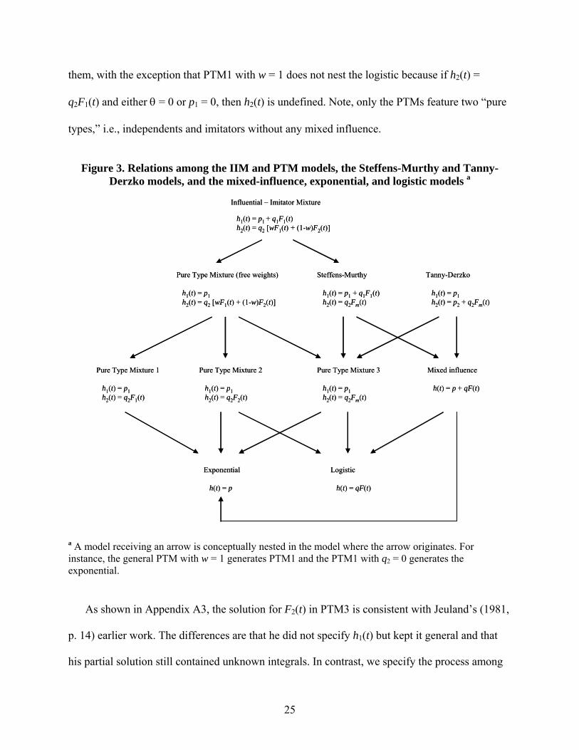
them, with the exception that PTM1 with w = 1 does not nest the logistic because if h2(t) =
q2F1(t) and either θ = 0 or p1 = 0, then h2(t) is undefined. Note, only the PTMs feature two “pure
types,” i.e., independents and imitators without any mixed influence.
Figure 3. Relations among the IIM and PTM models, the Steffens-Murthy and Tanny-
Derzko models, and the mixed-influence, exponential, and logistic models a
Exponential
h(t) = p
Logistic
h(t) = qF(t)
Mixed influence
h(t) = p + qF(t)
Pure Type Mixture 1
h1(t) = p1h2(t) = q2F1(t)
Pure Type Mixture 2
h1(t) = p1h2(t) = q2F2(t)
Pure Type Mixture 3
h1(t) = p1h2(t) = q2Fm(t)
Tanny-Derzko
h1(t) = p1h2(t) = p2 + q2Fm(t)
Steffens-Murthy
h1(t) = p1 + q1F1(t)h2(t) = q2Fm(t)
Pure Type Mixture (free weights)
h1(t) = p1h2(t) = q2 [wF1(t) + (1-w)F2(t)]
Influential – Imitator Mixture
h1(t) = p1 + q1F1(t)h2(t) = q2 [wF1(t) + (1-w)F2(t)]
a A model receiving an arrow is conceptually nested in the model where the arrow originates. For instance, the general PTM with w = 1 generates PTM1 and the PTM1 with q2 = 0 generates the exponential.
As shown in Appendix A3, the solution for F2(t) in PTM3 is consistent with Jeuland’s (1981,
p. 14) earlier work. The differences are that he did not specify h1(t) but kept it general and that
his partial solution still contained unknown integrals. In contrast, we specify the process among
25

independents and solve the equations using incomplete gamma functions, making parameter
estimation and empirical analysis possible.
5. Empirical analysis
To what extent does the two-segment IIM, consistent with several theoretical frameworks,
agree with empirical diffusion patterns? And how well does it do compared to the mixed-
influence model and other, more flexible, models? We provide insights on those issues through
an empirical analysis of 33 data series.
5.1. Data
One must use an informative variety of data sets if one is to draw sound conclusion on model
performance. We therefore analyze four sets of data. The first consists of a single series on the
diffusion of the broad-spectrum antibiotic tetracycline among 125 Midwestern physicians over a
period of 17 months in the mid-1950s. This series comes from the classic Medical Innovation
study (Coleman et al. 1966). It warrants special attention because it is commonly accepted as an
instance of diffusion in a mixture of independents and imitators (e.g., Jeuland 1981; Lekvall and
Wahlbin 1973; Rogers 2003).
The second set of data series consists of 19 music CDs, also a category where a two-segment
structure is a priori likely to exist. Some customers are dedicated fans buying products by their
favorite performers almost unconditionally (so q1 = 0 is quite possible), while others end up
buying the CD only after it has become popular and a must-buy (Farrell 1998; Yamada and Kato
2002). We use the weekly U.S. sales data analyzed previously by Moe and Fader (2001).9 Since
people are very unlikely to buy two identical CDs for themselves or to replace an older copy, the
sales data are unlikely to be contaminated by multiple or repeat purchases and can be treated as
9 The full set consists of 20 data series, but we deleted one that still had not reached the time of peak sales.
26
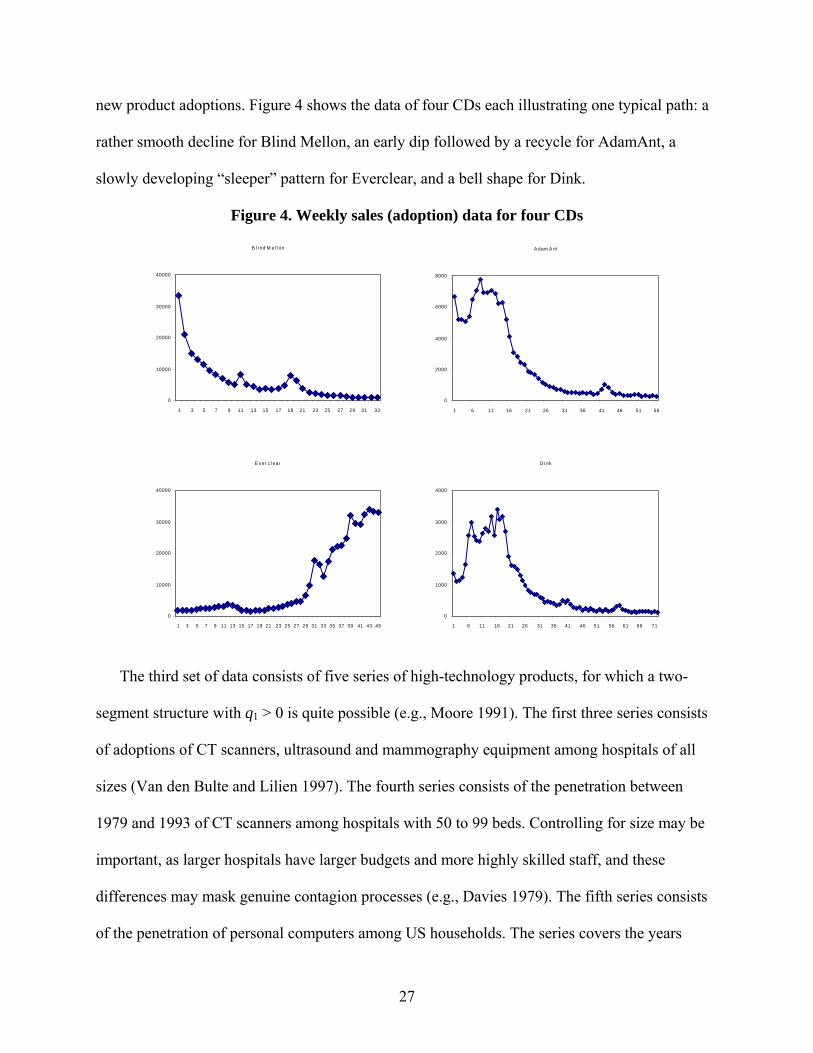
new product adoptions. Figure 4 shows the data of four CDs each illustrating one typical path: a
rather smooth decline for Blind Mellon, an early dip followed by a recycle for AdamAnt, a
slowly developing “sleeper” pattern for Everclear, and a bell shape for Dink.
Figure 4. Weekly sales (adoption) data for four CDs
A dam A nt
0
2000
4000
6000
8000
1 6 11 16 21 26 31 36 41 46 51 56
D i nk
0
1000
2000
3000
4000
1 6 11 16 21 26 31 36 41 46 51 56 61 66 71
B l i nd M el l on
0
10000
20000
30000
40000
1 3 5 7 9 11 13 15 17 19 21 23 25 27 29 31 33
E v er c l ear
0
10000
20000
30000
40000
1 3 5 7 9 11 13 15 17 19 21 23 25 27 29 31 33 35 37 39 41 43 45
The third set of data consists of five series of high-technology products, for which a two-
segment structure with q1 > 0 is quite possible (e.g., Moore 1991). The first three series consists
of adoptions of CT scanners, ultrasound and mammography equipment among hospitals of all
sizes (Van den Bulte and Lilien 1997). The fourth series consists of the penetration between
1979 and 1993 of CT scanners among hospitals with 50 to 99 beds. Controlling for size may be
important, as larger hospitals have larger budgets and more highly skilled staff, and these
differences may mask genuine contagion processes (e.g., Davies 1979). The fifth series consists
of the penetration of personal computers among US households. The series covers the years
27

1981-1996, but to avoid left-censoring artifacts we impose 1975 as the actual launch year. The
first three series are roughly bell-shaped, the latter two series show two “bells” separated by a
dip or “chasm”.
The final set is a miscellaneous mix of 8 data series analyzed previously by Van den Bulte
and Lilien (1997) and Bemmaor and Lee (2002) (these studies also included the tetracycline and
three of the high-tech series). There is no compelling a priori reason to expect a mixture of
independents and imitators to be able to account better for those diffusion data than traditional
models, and several innovations need not have diffused through contagion at all (Griliches 1962;
Van den Bulte and Stremersch 2004). The adoption curves all have a very pronounced bell
shape, with several showing skew that the MIM cannot account for (Bemmaor and Lee 2002).
5.2. Parameter estimates
Though we have closed-form solutions for both IIM and PTM, the solution to the IIM
involves Gaussian hypergeometric functions the estimation of which is very troublesome.10 We
therefore estimate the IIM not using the standard Srinivasan-Mason (1986) estimation approach
but through direct integration, that is, we compute non-linear least squares estimates at the same
time as we numerically solve the following differential equation11:
dX(t)/dt = M [θ f1(t) + (1−θ) f2(t) ] + ε(t)
= M [θ f1(t) + (1−θ) q2 {wF1(t)+(1-w) θ−
θ−1
)(/)( 1 tFMtX } {1-θ−
θ−1
)(/)( 1 tFMtX }] + ε(t)
[26] where X(t) is the cumulative number of adopters observed at time t, f1(t) and F1(t) are the closed-
form solutions to the adoption and penetration functions of the MIM, and f2(t) is expressed as in
10 Nonlinear regression in R and Mathematica either did not converge at standard convergence criteria or enabled us to obtain point estimates but not standard errors. We experienced these problems even with simulated data, which rules out model misspecification as an explanation for these difficulties. Maximum likelihood estimation is known to be troublesome as well, even when the parameters of interest enter the function linearly rather than non-linearly as in the IIM (e.g., Fader et al. 2005). 11 This can be done conveniently, e.g., using the model procedure in SAS or the odesolve package in R.
28

eq. (15), but with θ−
θ−1
)(/)( 1 tFMtX replacing F2(t). The latter is based on X(t) = MFm(t) (absent
error) and Fm(t) = θF1(t) + (1−θ)F2(t). We allow the error term ε(t) ∼ N(0,σ2) to exhibit serial
correlation up to order 2 when the time series contains more than 20 observations or the Durbin-
Watson statistic falls outside the 1.5-2.5 range. We impose that hazard parameters p1, q1, and q2
be non-negative (≥ 0) and that 0 ≤ θ ≤ 1. Because hazard rates can be larger than one in
continuous time, we do not impose p1, q1, and q2 ≤ 1. As to w, we impose 0.01% ≤ w ≤ 1,
choosing a very small but positive lower bound so the model itself ensures the “seeding” of the
contagion process among imitators.
Table 2 reports, for tetracycline, estimates obtained through direct integration (DI) for IIM,
PTM and MIM as well as those from the Srinivasan-Mason (SM) procedure for PTM and MIM.
Clearly, both procedures produce very similar estimates, though direct integration has somewhat
higher serial correlation because it fits the cumulative adoptions X(t) rather than the periodic
adoptions X(t) - X(t-1). The difference in dependent variable also explains why direct integration
produces higher R2 values. The parameter estimates of the IIM, with the zero value of q1
meaning that segment 1 consists of independents and the high value of θ meaning that contagion
affected only a minority, are consistent with previous analyses using individual-level data on
adoption times and actual network structure (Coleman et al. 1966; Van den Bulte and Lilien
2003), and so is the decomposition of total adoptions in Figure 5 (from PTM-SM re-estimated
without serial correlation). The graph indicates that by month 11, when 25% of all physicians
still had to adopt, all imitators had already adopted and the “laggards” consisted only of
independents. This is consistent with the original finding by Coleman et al. (1966) using
individual-level data that the laggards tended to be very poorly integrated in the social network
and hence unaffected by social influence. Finally, the mixture models generate an estimate of M
29
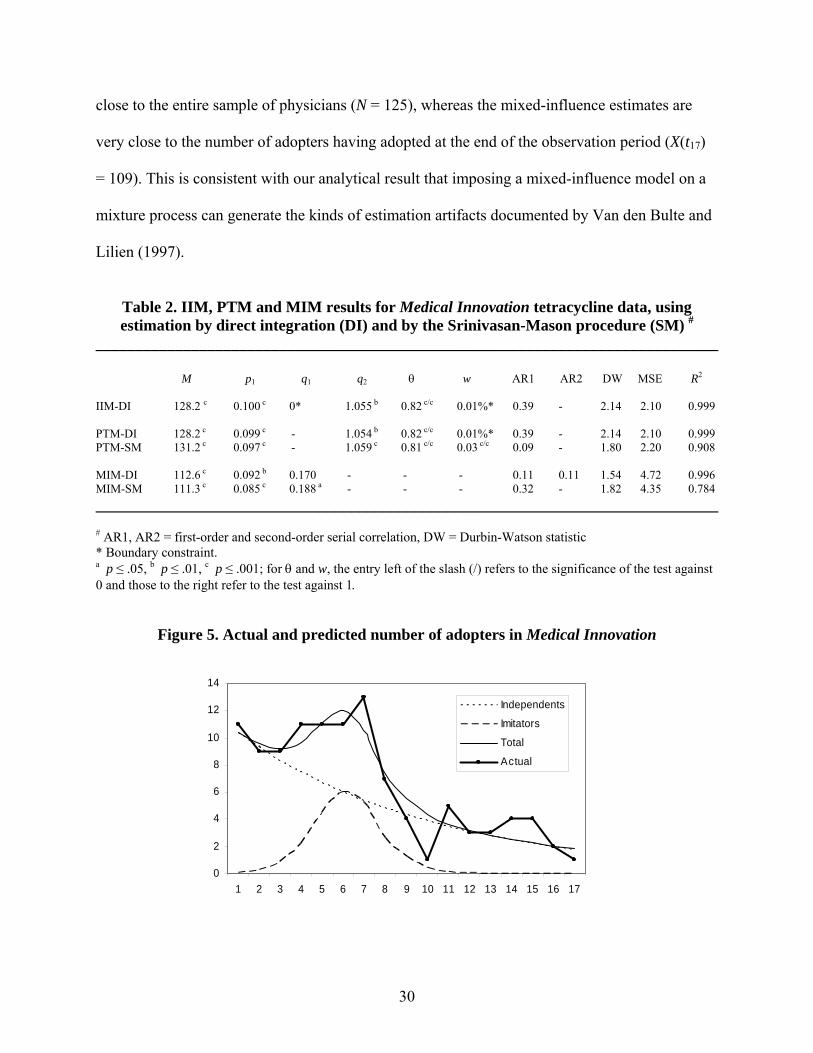
close to the entire sample of physicians (N = 125), whereas the mixed-influence estimates are
very close to the number of adopters having adopted at the end of the observation period (X(t17)
= 109). This is consistent with our analytical result that imposing a mixed-influence model on a
mixture process can generate the kinds of estimation artifacts documented by Van den Bulte and
Lilien (1997).
Table 2. IIM, PTM and MIM results for Medical Innovation tetracycline data, using estimation by direct integration (DI) and by the Srinivasan-Mason procedure (SM) #
______________________________________________________________________________
M p1 q1 q2 θ w AR1 AR2 DW MSE R2
IIM-DI 128.2 c 0.100 c 0* 1.055 b 0.82 c/c 0.01%* 0.39 - 2.14 2.10 0.999 PTM-DI 128.2 c 0.099 c - 1.054 b 0.82 c/c 0.01%* 0.39 - 2.14 2.10 0.999 PTM-SM 131.2 c 0.097 c - 1.059 c 0.81 c/c 0.03 c/c 0.09 - 1.80 2.20 0.908 MIM-DI 112.6 c 0.092 b 0.170 - - - 0.11 0.11 1.54 4.72 0.996 MIM-SM 111.3 c 0.085 c 0.188 a - - - 0.32 - 1.82 4.35 0.784 ______________________________________________________________________________ # AR1, AR2 = first-order and second-order serial correlation, DW = Durbin-Watson statistic * Boundary constraint. a p ≤ .05, b p ≤ .01, c p ≤ .001; for θ and w, the entry left of the slash (/) refers to the significance of the test against 0 and those to the right refer to the test against 1.
Figure 5. Actual and predicted number of adopters in Medical Innovation
0
2
4
6
8
10
12
14
1 2 3 4 5 6 7 8 9 10 11 12 13 14 15 16 17
Independents
Imitators
Total
Actual
30

Table 3 reports the results of estimating the IIM to all 33 data sets12. Values for p1 tend be
smaller than 0.3. There are two exceptions to this: Foreign Language where θ is so low that fm(0)
= θ p1 equals only 0.04, and the Beastie Boys CD that exhibited an extreme “blockbuster”
pattern, i.e., extremely quickly declining sales. Values for q1 show much more variance. This is
especially so for CDs. For about half of them, q1 equals zero, indicating the absence of word-of-
mouth among influentials. In four cases, q1 is larger than one, suggesting very strong word-of-
mouth among influentials. However, these large estimates are very imprecise and only one is
significant at 95% confidence. Values for q2 also show considerable variance, with several high
values recorded for the set of miscellaneous innovations. These high values may result from the
strong left skew in the adoption time series without implying the presence of true contagion
(Bemmaor and Lee 2002). Finally, θ is often significantly different from both 0 and 1, indicating
that the IIM does not reduce to the mixed-influence or logistic models, and only weakly
correlated with w (r = -.14). That θ is often larger than 2.5% or 16%, traditional values used to
separate innovators from imitators based on time of adoption, is an indication—in addition to the
φ(t) function and the results for Medical Innovation—that the dichotomy based on drivers of
adoption underlying the IIM is conceptually different from that based on time of adoption. Since
it may be of particular interest, we show in Figure 6 that the IIM can indeed capture bimodal
patterns in real data.
5.3. Descriptive performance
To assess the descriptive performance of the two-segment model, we compare it against that
of the mixed-influence (MIM), Gamma/Shifted Gompertz (G/SG), Weibull-Gamma (WG), and
Karmeshu-Goswami (KG) models. Since all these models have a closed-form solution, we
12 We do not report the ceiling parameter values M due to space constraints.
31
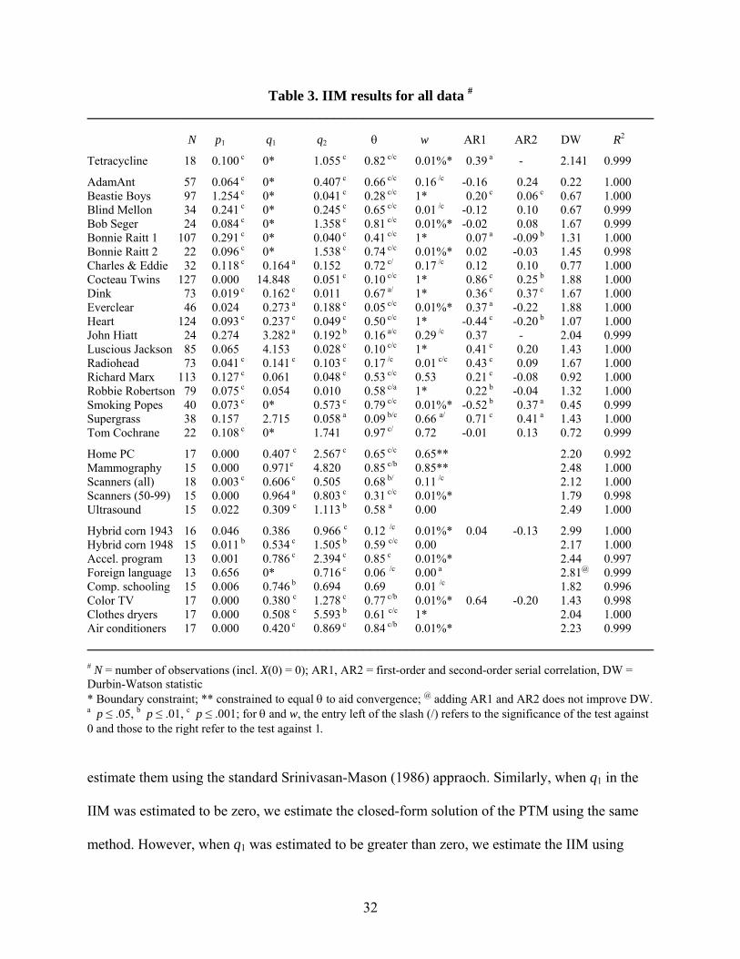
Table 3. IIM results for all data #______________________________________________________________________________ N p1 q1 q2 θ w AR1 AR2 DW R2
Tetracycline 18 0.100 c 0* 1.055 c 0.82 c/c 0.01%* 0.39 a - 2.141 0.999
AdamAnt 57 0.064 c 0* 0.407 c 0.66 c/c 0.16 /c -0.16 0.24 0.22 1.000 Beastie Boys 97 1.254 c 0* 0.041 c 0.28 c/c 1* 0.20 c 0.06 c 0.67 1.000 Blind Mellon 34 0.241 c 0* 0.245 c 0.65 c/c 0.01 /c -0.12 0.10 0.67 0.999 Bob Seger 24 0.084 c 0* 1.358 c 0.81 c/c 0.01%* -0.02 0.08 1.67 0.999 Bonnie Raitt 1 107 0.291 c 0* 0.040 c 0.41 c/c 1* 0.07 a -0.09 b 1.31 1.000 Bonnie Raitt 2 22 0.096 c 0* 1.538 c 0.74 c/c 0.01%* 0.02 -0.03 1.45 0.998 Charles & Eddie 32 0.118 c 0.164 a 0.152 0.72 c/ 0.17 /c 0.12 0.10 0.77 1.000 Cocteau Twins 127 0.000 14.848 0.051 c 0.10 c/c 1* 0.86 c 0.25 b 1.88 1.000 Dink 73 0.019 c 0.162 c 0.011 0.67 a/ 1* 0.36 c 0.37 c 1.67 1.000 Everclear 46 0.024 0.273 a 0.188 c 0.05 c/c 0.01%* 0.37 a -0.22 1.88 1.000 Heart 124 0.093 c 0.237 c 0.049 c 0.50 c/c 1* -0.44 c -0.20 b 1.07 1.000 John Hiatt 24 0.274 3.282 a 0.192 b 0.16 a/c 0.29 /c 0.37 - 2.04 0.999 Luscious Jackson 85 0.065 4.153 0.028 c 0.10 c/c 1* 0.41 c 0.20 1.43 1.000 Radiohead 73 0.041 c 0.141 c 0.103 c 0.17 /c 0.01 c/c 0.43 c 0.09 1.67 1.000 Richard Marx 113 0.127 c 0.061 0.048 c 0.53 c/c 0.53 0.21 c -0.08 0.92 1.000 Robbie Robertson 79 0.075 c 0.054 0.010 0.58 c/a 1* 0.22 b -0.04 1.32 1.000 Smoking Popes 40 0.073 c 0* 0.573 c 0.79 c/c 0.01%* -0.52 b 0.37 a 0.45 0.999 Supergrass 38 0.157 2.715 0.058 a 0.09 b/c 0.66 a/ 0.71 c 0.41 a 1.43 1.000 Tom Cochrane 22 0.108 c 0* 1.741 0.97 c/ 0.72 -0.01 0.13 0.72 0.999
Home PC 17 0.000 0.407 c 2.567 c 0.65 c/c 0.65** 2.20 0.992 Mammography 15 0.000 0.971c 4.820 0.85 c/b 0.85** 2.48 1.000 Scanners (all) 18 0.003 c 0.606 c 0.505 0.68 b/ 0.11 /c 2.12 1.000 Scanners (50-99) 15 0.000 0.964 a 0.803 c 0.31 c/c 0.01%* 1.79 0.998 Ultrasound 15 0.022 0.309 c 1.113 b 0.58 a 0.00 2.49 1.000
Hybrid corn 1943 16 0.046 0.386 0.966 c 0.12 /c 0.01%* 0.04 -0.13 2.99 1.000 Hybrid corn 1948 15 0.011 b 0.534 c 1.505 b 0.59 c/c 0.00 2.17 1.000 Accel. program 13 0.001 0.786 c 2.394 c 0.85 c 0.01%* 2.44 0.997 Foreign language 13 0.656 0* 0.716 c 0.06 /c 0.00 a 2.81@ 0.999 Comp. schooling 15 0.006 0.746 b 0.694 0.69 0.01 /c 1.82 0.996 Color TV 17 0.000 0.380 c 1.278 c 0.77 c/b 0.01%* 0.64 -0.20 1.43 0.998 Clothes dryers 17 0.000 0.508 c 5.593 b 0.61 c/c 1* 2.04 1.000 Air conditioners 17 0.000 0.420 c 0.869 c 0.84 c/b 0.01%* 2.23 0.999 ______________________________________________________________________________ # N = number of observations (incl. X(0) = 0); AR1, AR2 = first-order and second-order serial correlation, DW = Durbin-Watson statistic * Boundary constraint; ** constrained to equal θ to aid convergence; @ adding AR1 and AR2 does not improve DW. a p ≤ .05, b p ≤ .01, c p ≤ .001; for θ and w, the entry left of the slash (/) refers to the significance of the test against 0 and those to the right refer to the test against 1. estimate them using the standard Srinivasan-Mason (1986) appraoch. Similarly, when q1 in the
IIM was estimated to be zero, we estimate the closed-form solution of the PTM using the same
method. However, when q1 was estimated to be greater than zero, we estimate the IIM using
32
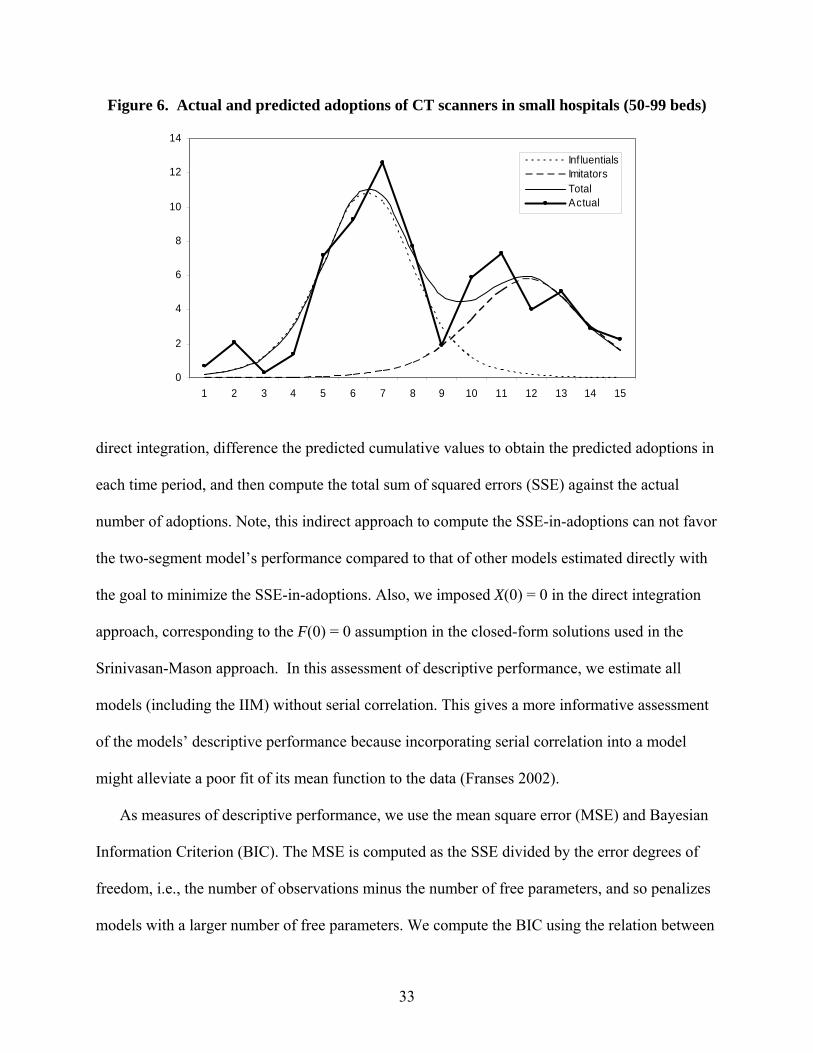
Figure 6. Actual and predicted adoptions of CT scanners in small hospitals (50-99 beds)
0
2
4
6
8
10
12
14
1 2 3 4 5 6 7 8 9 10 11 12 13 14 15
Inf luentialsImitatorsTotalActual
direct integration, difference the predicted cumulative values to obtain the predicted adoptions in
each time period, and then compute the total sum of squared errors (SSE) against the actual
number of adoptions. Note, this indirect approach to compute the SSE-in-adoptions can not favor
the two-segment model’s performance compared to that of other models estimated directly with
the goal to minimize the SSE-in-adoptions. Also, we imposed X(0) = 0 in the direct integration
approach, corresponding to the F(0) = 0 assumption in the closed-form solutions used in the
Srinivasan-Mason approach. In this assessment of descriptive performance, we estimate all
models (including the IIM) without serial correlation. This gives a more informative assessment
of the models’ descriptive performance because incorporating serial correlation into a model
might alleviate a poor fit of its mean function to the data (Franses 2002).
As measures of descriptive performance, we use the mean square error (MSE) and Bayesian
Information Criterion (BIC). The MSE is computed as the SSE divided by the error degrees of
freedom, i.e., the number of observations minus the number of free parameters, and so penalizes
models with a larger number of free parameters. We compute the BIC using the relation between
33

the SSE and the concentrated log-likelihood which allows one to compute likelihood ratios and
other statistics based on the model likelihood from the SSE (Seber and Wild 1989). To aid
interpretation, we report only the ratio of the baseline models’ MSE to that of the two-segment
model. This relative measure controls for the total variance in the data, with 1 being the neutral
value and higher values indicating superior fit of the two-segment model. Similarly, we report
only the difference in BIC, with 0 being the neutral value and higher values indicating superior
fit of the two-segment model.
Table 4 reports the performance indicators averaged for each of the four sets of data as well
as for all 33 data series (Appendix A4 reports results for the individual series). The MSE ratios
indicate that the two-segment model fits markedly better than the MIM, G/SG and WG models,
the latter having an MSE that is 60% to 96% higher. Importantly, the model fits better for
tetracycline, high-tech, and music CDs, but not for the miscellaneous products where the
presumption of a discrete mixture is not strong a priori. The two-segment model outperforms the
continuous-mixture KG model by only a moderate margin for tetracycline and the high-tech
products. The same set of conclusions flow from using the BIC difference, where a 3-point
difference is large enough to be evidence of superior fit and a 10-point difference provides strong
to very strong evidence of superior fit (Raftery 1995). The one difference between the BIC and
MSE analysis is that the G/SG and WG models do not underperform as much on the BIC as on
the MSE for the high-tech products.
34

Table 4. Descriptive performance of two-segment models compared to mixed-influence, Gamma/Shifted Gompertz, Weibull-Gamma, and Karmeshu-Goswami models #
______________________________________________________________________________
MSE ratio BIC difference
MIM G/SG WG KG MIM G/SG WG KG
Tetracycline 2.06 2.22 2.38 1.36 9.23 12.07 13.24 7.77 Music CDs 2.27 1.98 1.91 0.93 47.57 40.02 23.75 0.79 High-tech 2.18 1.42 1.51 1.19 8.56 2.55 3.11 3.04 Miscellaneous 1.30 1.00 1.17 1.08 2.18 -0.71 1.46 2.52
All 1.96 1.59 1.63 1.02 28.93 23.11 14.12 1.79 ______________________________________________________________________________ # To save space and aid interpretation, we report only the alternative models’ MSE divided by that of the two-segment model, and the alternative models’ BIC minus that of the two-segment model. For the MSE ratio, the neutral value is 1; for the BIC difference, it is 0. For both metrics, higher values indicate superior fit of the two-segment model. For the MSE ratio, the geometric mean is reported as this is a better measure of central tendency of a ratio than the arithmetic mean. For the BIC difference, the latter is reported. 6. Conclusion
We have modeled the diffusion of innovations in a social structure that is of increasing
interest to marketing practitioners as well as academics: a two-segment structure with influentials
who are more in touch with new developments, who may but need not act independently from
each other, and who affect another segment of pure imitators whose own adoptions do not affect
the influentials. Such a two-segment structure is consistent with several theories in sociology and
diffusion research, including the classic two-step flow hypothesis and Moore’s more recent
technology adoption framework. Our model allows diffusion researchers to operationalize these
theories without recourse to micro-level diffusion data and to estimate parameters from real data.
There are four main results.
(1) Diffusion in a mixture of influentials and imitators can exhibit the traditional symmetric-
around-the-peak bell shape, asymmetric bell shapes, as well as a dip or “chasm” between the
early and later parts of the diffusion curve. In contrast to Moore’s contention, the model suggests
that it need not always be necessary to change the product to gain traction among later adopters
35

and the adoption curve to swing up again. Tetracycline is an example. Hence, we provide closed-
form corroboration for the result Goldenberg et al. (2002) obtained from a simulation study. The
management implication is that launching a new version to appeal to prospects who have not
adopted yet need not be necessary, let alone optimal, to get out of the dip.
(2) The proportion of adoptions stemming from independents need not decrease
monotonically; it can also first decline and then rise again to unity. This rejects a still common
contention based on an erroneous mixture interpretation of the mixed-influence model. The
management implication is that, while it may make sense to shift the focus of one’s marketing
efforts from independents to imitators shortly after launch as shown by Mahajan and Muller
(1998) using a two-period model, one may want to start increasing one’s resource allocation to
independent decision makers again later in the process.
(3) Specifying a mixed-influence model to a mixture process where influentials act
independently from each other (q1=0) can generate systematic changes in the parameter values.
As several authors have noted, diffusion within a pure-type mixture of independents and
imitators with hazards p and qF(t), respectively, is distinct from diffusion in a homogenous
population with mixed-influence where everyone adopts with hazard p + qF(t). The closed-form
solutions we present not only prove this mathematically but also show that unless θ is close to
either 0 or 1, imposing a mixed-influence specification on a pure-type mixture process can
generate the systematic changes in the parameter values reported by Van den Bulte and Lilien
(1997), Bemmaor and Lee (2002), and Van den Bulte and Stremersch (2004).
(4) Empirical analysis of four sets of data comprising a total of 33 different data series (the
classic Medical Innovation data, 19 music CDs, 5 high-tech products, and 8 miscellaneous
innovations) indicates that the two-segment model fits markedly better than the mixed-influence,
36

the Gamma/Shifted Gompertz, and the Weibull-Gamma model, at least in cases where a two-
segment structure is likely to exist. Hence, the model does better when it is theoretically
expected to and does not when it is not theoretically expected to. The two-segment model fits
only somewhat better, but certainly not worse, than the mixed-influence model recently proposed
by Karmeshu and Goswami (2001) where p and q vary in a continuous fashion. Specifically, the
two-segment model outperforms the continuous-mixture KG model by a moderate margin in two
of the four cases (tetracycline and the high-tech products) and matches it in the other two cases
(music CDs and miscellaneous innovations). Overall, the differences in descriptive performance
indicate that the discrete-mixture model is sufficiently different and the data sufficiently
informative for the model to fit real data better than other models.
The models we presented provide sharper insight into how social structure can affect macro-
level diffusion patterns, and should prove useful in three areas of application where influentials
and imitators are a priori likely to exist. The first area is that of high-technology products, where
there is a strong interest in the potential existence of “early market” independents and
“mainstream” imitators. The second area is that of movies, a category that has attracted the
attention of many researchers recently.13 The third area consists of situations where a segment of
enthusiasts has pent-up demand. For instance, when internet access providers started operating in
France in 1996, a rather large number of people adopted their services. New adoptions dipped in
13 Explicitly allowing for influentials and imitators may be especially useful for movies carried by actors or directors who already have a small following among aficionados but have not yet broken through to the mainstream audience. In such cases, one would expect the former to adopt according an independent process and the latter to adopt only through contagion, if at all. This might result in a temporary dip. Movies starring Christina Ricci and movies directed by Ang Lee exhibit this pattern. Early in her career, Christina Ricci played in several independent movies that won critical acclaim and earned her the label of “Indie Queen”. These early movies exhibited the bell curve typical of very successful “sleepers” (The Ice Storm-1997; The Opposite of Sex-1998; Buffalo 66-1998). Then followed a small movie exhibiting a dip (Desert Blue-1998), while her recent movies are more standard Hollywood fare exhibiting the standard monotonic, exponential decline (e.g., The Man Who Cried-2001). The same pattern is observed for movies directed by Ang Lee:bell-shaped for The Ice Storm-1997, a temporary dip for Ride with the Devil-1999, and monotonic decline for his more recent Hollywood production The Hulk-2003.
37

1997, only to increase again from 1998 onwards. The deviation form the standard bell shape was
not the low number in 1997 but the high initial number in 1996, when many university users who
had been accessing the internet exclusively through the university RENATER network were
finally able to start using the internet at home as well (Fornerino 2003). In case the enthusiasts
can place advance orders that the marketing analyst can observe (e.g., Moe and Fader 2002), it
may be useful to explicitly allow for a difference between the start time of the diffusion process
of the two segments.
An important extension of our work would be to incorporate control variables, including
marketing mix efforts. This may not only be useful for empirical research, but may also enable
one to study the decision to target independents versus imitators in continuous time. Even a
simplified three-period model might be helpful in studying under what conditions it is profit
maximizing to change one’s targeting from independents to imitators and, possibly, to
independents again (cf. Mahajan and Muller 1998). Like the models we presented, this extension
would allow one to better understand current arguments and findings, to formalize richer
theoretical arguments, and perhaps even to operationalize them into estimable models that help
bridge the gap between theory and data.
38

References
Bass, Frank M. 1969. A new product growth model for consumer durables. Management Sci. 15 215-227.
Becker, Marshall H. 1970. Sociometric location and innovativeness: Reformulation and
extension of the diffusion model. Am. Sociological Rev. 35 267-283. Bemmaor, Albert C. 1994. Modeling the diffusion of new durable goods: Word-of-mouth effect
versus consumer heterogeneity. Gilles Laurent, Gary L. Lilien, Bernard Pras, eds. Research Traditions in Marketing. Kluwer Academic Publishers, Boston, MA, 201-223.
Bemmaor, Albert C., Yanghyuk Lee. 2002. The impact of heterogeneity and ill-conditioning on
diffusion model parameter estimates. Marketing Sci. 21 209-220. Bourdieu, Pierre. 1984. Distinction: A Social Critique of the Judgment of Taste. Harvard
University Press, Cambridge, MA. Bronnenberg, Bart J., Carl F. Mela. 2004. Market roll-out and retailer adoption for new brands.
Marketing Sci. 23 50-518. Burt, Ronald S. 1987. Social contagion and innovation: Cohesion versus structural equivalence.
Amer. J. Sociology 92 1287-1335. Cancian, Frank. 1979. The Innovator’s Situation: Upper-Middle-Class Conservatism in
Agricultural Communities. Stanford University Press, Stanford, CA. Case, Anne C., Harvey S. Rosen, James R. Hines. 1993. Budget spillovers and fiscal policy
interdependence. J. Public Econom. 52 285-307. . Coleman, James S. 1964. Introduction to Mathematical Sociology. The Free Press of Glencoe,
London, UK. Coleman, James S., Elihu Katz, Herbert Menzel. 1966. Medical Innovation: A Diffusion Study.
Bobbs-Merrill Company, Indianapolis, IN. Coulter, Robin A., Lawrence Feick, Linda L. Price. 2002. Changing faces: Cosmetics opinion
leadership among women in the new Hungary. Eur. J. Marketing 36 1287-1308. Cox, D.R. 1959. The analysis of exponentially distributed life-times with two types of failure. J.
Roy. Stat. Soc. B 21 411-421. Daley, D.J. 1967. Concerning the spread of news in a population of individuals who never forget.
Bull. Math. Biophys. 29 373-376.
39

Davies, Stephen. 1979. The Diffusion of Process Innovations. Cambridge University Press, Cambridge, UK.
Dixon, Robert. 1980. Hybrid corn revisited. Econometrica 46 1451-1461. Ehrenreich, Barbara. 1989. Fear of Falling: The Inner Life of the Middle Class. Pantheon Books,
New York, NY. Fader, Peter S., Bruce G.S. Hardie, Ka Kok Lee. 2005. “Counting your customers” the easy way:
An alternative to the Pareto/NBD model. Marketing Sci. 24 275-284. Farrell, Winslow. 1998. How Hits Happen. HarperCollins, New York, NY. Fornerino, Marianela. 2003. Internet adoption in France. Serv. Ind. J. 23 119-135. Franses, Philip Hans. 2002. Testing for residual autocorrelation in growth curve models. Tech.
Forecasting Soc. Change 69 195-204. Frenzen, Jonathan K., Kent Nakamoto. 1993. Structure, cooperation, and the flow of market
information. J. Consumer Res. 20 360-375. Gladwell, Malcolm. 2000. The Tipping Point. Little, Brown and Company, New York, NY. Goldenberg, Jacob, Barak Libai, Eitan Muller. 2002. Riding the saddle: How cross-market
communications can create a major slump in sales. J. Marketing 66 (2), 1-16. Griliches, Zvi. 1962. Profitability versus interaction: Another false dichotomy. Rural Sociol. 27
327-330. Hardie, Bruce G.S., Peter S. Fader, Michael Wisniewski. 1998. An empirical comparison of new
product trial forecasting models. J. Forecasting 17 209-229. Haunschild, Pamela R., Anne S. Miner. 1997. Modes of interorganizational imitation: The
effects of outcome salience and uncertainty. Admin. Sci. Quart. 42 472-500. Hernes, Gudmund. 1976. Diffusion and growth—The non-homogenous case. Scand. J. Econ. 78
427-436. Homans, George C. 1960. Social Behavior: Its Elementary Forms. Harcourt, Brace, and World,
New York, NY. Jeuland, Abel P. 1981. Parsimonious models of diffusion of innovation. Part A: Derivations and
comparisons. Working paper, University of Chicago, Chicago, IL. Karmeshu, Debasree Goswami. 2001. Stochastic evolution of innovation diffusion in
heterogeneous groups: Study of life cycle patterns, IMA J. Manage. Math. 12 107-126.
40

Katz, Elihu. 1957. The two-step flow of communication: An up-to-date report on an hypothesis.
Public Opin. Quart. 21 61-78. Katz, Elihu, Paul F. Lazarsfeld. 1955. Personal Influence: The Part Played by People in the
Flow of Mass Communication. The Free Press, Glencoe, IL. Keller, Ed, Jon Berry. 2003. The Influentials. Free Press, New York, NY. Lazarsfeld, Paul F., Bernard Berelson, Hazel Gaudet. 1944. The People’s Choice: How the Voter
Makes Up His Mind in a Presidential Campaign. Duell, Sloan and Pearce, New York. Lekvall, Per, Clas Wahlbin. 1973. A study of some assumptions underlying innovation diffusion
functions. Swed. J. Econ. 75 362-377. Lilien, Gary L., Ambar Rao, Shlomo Kalish. 1981. Bayesian estimation and control of detailing
effort in a repeat purchase diffusion environment. Management Sci. 27 493-506. Maffesoli, Michel. 1996. The Time of the Tribes: The Decline of Individualism in Mass Society.
Sage, London, U.K. Mahajan, Vijay, Eitan Muller. 1998. When is it worthwhile targeting the majority instead of the
innovators in a new product launch? J. Marketing Res. 35 488-495. Mahajan, Vijay, Eitan Muller, Frank M. Bass. 1993. New-product diffusion models. J.
Eliashberg, G.L. Lilien, eds. Marketing (Handbooks in Operations Research and Management Science, Vol. 5). North-Holland, Amsterdam, Netherlands, 349-408.
Mahajan, Vijay, Eitan Muller, Rajendra K. Srivastava. 1990. Determination of adopter categories
by using innovation diffusion models. J. Marketing Res. 27 37-50. Mahajan, Vijay, Robert A. Peterson. 1985. Models for Innovation Adoption. Sage, Newbury
Park, CA. Manfredi, Piero, Andrea Bonaccorsi, Angelo Secchi. 1998. Social heterogeneities in classical
new product diffusion models. I: “external” and “internal” models. Technical Report No. 174, Dipartimento Statistica e Matematica Applicata all’Economia, Università di Pisa, Pisa, Italy.
Mansfield, Edwin. 1961. Technical change and the rate of imitation. Econometrica 29 741-766. Massy, William F, David B. Montgomery, Donald G. Morrison. 1970. Stochastic Models of
Buying Behavior. MIT Press, Cambridge. MA.
41

Merton, Robert K. 1949. Patterns of influence: A study of interpersonal influence and communications behavior in a local community. Paul F. Lazarsfeld, Frank N. Stanton, eds. Communications Research, 1948-1949. Harper & Brothers, New York, 180-219.
Midgley, David F., Grahame R. Dowling. 1978. Innovativeness: The concept and its
measurement. J. Consumer Res. 4 229-242. Miller, Christopher M., Shelby H. McIntyre, Murali K. Mantrala. 1993. Toward formalizing
fashion theory. J. Marketing Res. 30 (2) 142-157. Moe, Wendy W., Peter S. Fader. 2001. Modeling hedonic portfolio products: A joint
segmentation analysis of music compact disc sales. J. Marketing Res. 38 376-385. Moe, Wendy W., Peter S. Fader. 2002. Using advance purchase orders to forecast new product
sales. Marketing Sci. 21 347-364. Moore, Geoffrey A. 1991. Crossing the Chasm. HarperBusiness, New York, NY. Moore, Geoffrey A. 1995. Inside the Tornado. HarperBusiness, New York, NY. Moorthy, K. Sridhar. 1993. Theoretical modeling in marketing. J. Marketing 57 (2) 92-106. Myers, James H., Thomas S. Robertson. 1972. Dimensions of opinion leadership. J. Marketing
Res. 9 41-46. Narayanan, Sunder. 1992. Incorporating heterogeneous adoption rates in new product diffusion
models: A model and empirical investigations. Marketing Lett. 3 395-406. Philips, Damon J., Ezra W. Zuckerman, 2001. Middle-status conformity: Theoretical restatement
and empirical demonstration in two markets. Amer. J. Sociol. 107 379-429. Putsis, William P., Jr., Sridhar Balasubramaniam, Edward H. Kaplan, Subrata K. Sen. 1997.
Mixing behavior in cross-country diffusion. Marketing Sci. 16 354-369. Raftery, Adrian E. 1995. Bayesian model selection in social research. Peter V. Marsden, ed.
Sociological Methodology 1995. Blackwell, Oxford, U.K., 111-163. Riesman, David. 1950. The Lonely Crowd: A Study of the Changing American Character. Yale
University Press, New Haven, CT. Rogers, Everett M. 2003. Diffusion of Innovations, 5th ed. Free Press, New York, NY. Rosen, Emanuel. 2000. The Anatomy of Buzz. Doubleday, New York, NY. Schor, Juliet B. 1998. The Overspent American: Upscaling, Downshifting, and the New
Consumer. Basic Books, New York, NY.
42
Seber, G.A.F., C.J. Wild. 1989. Nonlinear Regression. John Wiley, New York, NY. Silk, Alvin J. 1966. Overlap among self-designated opinion leaders: A study of selected dental
products and services. J. Marketing Res. 3 255-259. Simmel, Georg.1971. Fashion. Donald N. Levine, ed. Georg Simmel on Individuality and Social
Forms. University of Chicago Press, Chicago, IL, 294-323. Slywotzky, Adrian J., Benson P. Shapiro. 1993. Leveraging to beat the odds: The new marketing
mind-set. Harvard Bus. Rev. 71 (5) 97-107. Srinivasan, V., Charlotte H. Mason. 1986. Nonlinear least squares estimation of new product
diffusion models. Marketing Sci. 5 169-178. Steffens, P.R., D.N.P. Murthy. 1992. A mathematical model for new product diffusion: The
influence of innovators and imitators. Math. Comput. Model. 16 (4), 11-26 Taga, Yasushi, Keiiti Isii. 1959. On a stochastic model concerning the pattern of communication:
Diffusion of news in a social group. Ann. I. Stat. Math. 11 25-43. Tanny, S.M., N.A. Derzko. 1988. Innovators and imitators in innovation diffusion modeling. J.
Forecasting 7 225-234. Valente, Thomas W., Beth R. Hoffman, Annamara Ritt-Olson, Kara Lichtman, C. Anderson
Johnson. 2003. Effects of a social-network method for group assignment strategies on peer-led tobacco prevention programs in schools. Am. J. Public Health 93 1837-1843
Van den Bulte, Christophe, Gary L. Lilien. 1997. Bias and systematic change in the parameter
estimates of macro-level diffusion models. Marketing Sci. 16 338-353. Van den Bulte, Christophe, Gary L. Lilien. 2001. Medical Innovation revisited: Social contagion
versus marketing effort. Amer. J. Sociol. 106 1409-1435. Van den Bulte, Christophe, Gary L. Lilien. 2003. Two-stage partial observability models of
innovation adoption. Working paper, University of Pennsylvania, Philadelphia, PA. Van den Bulte, Christophe, Stefan Stremersch. 2004. Social contagion and income heterogeneity
in new product diffusion: A meta-analytic test. Marketing Sci. 23 530-544. Williams, Ross A. 1972. Growth in ownership of consumer durables in the United Kingdom.
Economica (New Series) 39 60-69. Yamada, Masataka, Hiroshi Kato. 2002. A structural analysis of sales patterns of music CDs.
Presentation at the 2002 INFORMS Marketing Science Conference, University of Alberta, Edmonton, AB, Canada, June 27-30.
43

Appendix
A.1. Solution for F2(t) in IIM: h1(t) = p1 + q1F1(t) and h2(t) = q2[wF1(t)+(1-w)F2(t)]
To simplify notation, we omit the time argument from functions and write instead of
etc. We know
1F ),(1 tF
)1/()1( )()(1
11
1
111 tqppqtqp eeF +−+− +−= . Since ),)1(( 2122 FwwFqh −+= we write:
2222
1
12
1
12
2 )1()1(1
1
11
1
1
11
)11(
)(
)11(
)( FwqFwwqwqdtdF
p
tqpeq
tqp
p
tqpeq
tqp ee −−−−+= +−
+−
+−
+−
+
−
+
− [A.1.1]
A.1.1 is a Ricatti equation of the general form 2)()()( yxRyxQxPdxdy
++= .
Setting and 2Fy = ,tx = we get 1
1
11
)11(
)(
1
12)(
p
tqpeq
tqpewqxP +−
+−
+
−= ; )1()(1
1
11
)11(
)(
1
12
p
tqpeq
tqpewwqxQ +−
+−
+
−−−= ; and
is a potential solution for this Ricatti equation. We use the
transformation
).1()( 2 wqxR −−= 12 =F
zzF
Fz 1
11
22
+=⇒
−= . For continuous in is continuous in 2F ],1,0[ z ].1,( −−∞
Note, dtdz
zdtdF
22 1
−= . The equation now becomes:
)1()1(1
1
11
)11(
)(
1
122
p
tqpeq
tqpewwzqwqdtdz
+−
+−
+
−+−+−= [A.1.2]
This is of the form )()( 11 xQxPdxd
=+ µµ with µ=z; x=t; )1()(1
1
11
)11(
)(
1
121
p
tqpeq
tqpewwqxP +−
+−
+
−+−−= ; and
The general solution for such an equation is ).1()( 21 wqxQ −=)()()( 1
xucdxxQxu +∫=µ where
is the integrating factor. ))(exp()( 1 dxxPxu ∫=
Since ),ln()( )(1121
11
1
2 tqpq
wq eqptqdxxP +−+−−=∫ we get )).ln(exp()( )(112
11
1
2 tqpq
wq eqptqxu +−+−−=
A- 1

Hence, )1()1()(
111
1
2
11111
21
)(
)().( wqwpHweqpqe q
wqtqptq
dxxQxu −−−+
−+−−
=∫ , where
);1;,1( )11(11
1
11
2
1
2
1
2121 tqpeqp
pqp
wqq
wqFH +−++−+= and 2F1(1,b;c;k) is the Gaussian hypergeometric
function, the series representation of which is given by ∑∞
= +ΓΓΓ+Γ
0 )()()()(
n
nkncbcnb . This series is
convergent for arbitrary b, c when |k| < 1; and for k = ±1 when c > 1 + b. This implies that the
series is convergent as long as q1 > 0.
Substituting back, we get ))ln(exp( )(
112
)1()1()(
11
1
2
11
112
)11(111
2
tqpq
wqwqwp
Hweqpqe
eqptqc
zq
wqtqptq
+−−−
−+
+−−
+=
−+−−
Transforming back to we obtain z ,2F
c
eqptqF
wqwpHweqpqe
tqpq
wq
qwq
tqptq
+
+−−+=
−−−+
+−
−+−−
)1()1()(
)(112
2
11
112
)11(111
2
11
1
2 ))ln(exp(1 [A.1.3]
Since ,0)0(2 =F )1())1()1(()(
11
2111111
2
wqwpHwqwpwqqp q
wq
c −−−−−−+
−
= , where
);1;,1(11
1
11
2
1
2
1
2122 qp
pqp
wqq
wqFH++
−+= . Simplifying, we obtain as closed-form expression:
))1()1(()()1(
)1(1)(
211111
112
12
11
)11(112 HwqwpwqeHwq
wqwptFq
wqtqp
qpeqptq −−−−+−
−−+=
++ +−
[A.1.4]
A.2. Solution for F2(t) in PTM: h1(t) = p1 and h2(t) = q2[wF1(t)+(1-w)F2(t)]
Note: to simplify the notation, we replace p1 by p and q2 by q. We know that and
that
pteF −−= 11
]1][)1([ 2212
2 FFwwFqdt
dFf −−+== , and so write
222
2 )1()21()1( FwqFwewqeqwdt
dF ptpt −−+−+−= −− [A.2.1]
A- 2

The above equation is a Ricatti equation of the general form:
2)()()( yxRyxQxPdxdy
++= [A.2.2]
Setting y=F2 and x=t, we get ; ; and
. F
)1()( pteqwxP −−= )21()( ptwewqxQ −+−=
)1()( wqxR −−= 2 = 1 is a potential solution for Eq[A.2.2]. We use the transformation
zzF
Fz 1
11
22
+=⇒
−= . For F2 continuous in [0,1], z is continuous in (-∞,-1]. Note
dtdz
zdtdF
22 1
−= . After substitution, we can write Eq[A.2.1] as
)1()1( ptwezqwqdtdz −−+−= [A.2.3]
Eq[A.2.3] is of the form: )()( 11 xQxPdxd
=+ µµ , with µ = z; x = t; ; and
. Again, the general solution for such an equation is
)1()(1ptweqxP −−−=
)1()(1 wqxQ −=
)()()( 1
xucdxxQxu +∫=µ [A.2.4]
where is the integrating factor. ))(exp()( 1 dxxPxu ∫=
Sincep
qweqtdxxPpt
−+−=
−
∫ )(1 , we get )exp()( ptwepqqtxu −−−= ; and hence
dtwqwepqqtdxxQxu pt )1()exp()()( 1 −−−= −∫∫ . Now let us define
dtwepqqtwqI pt )exp()1( −−−−= ∫ [A.2.5]
To solve this integral, we do another transformation: dapa
dtap
te pt 1ln1a −=⇒−=⇒= − .
Eq[A.2.5] then becomes dawapqaw
pqI p
q
)exp()1(1
−−−=−
∫ , the solution to which is
),())(1( wapq
pqw
pqw
pqI p
q
Γ−=−
[A.2.6]
where Γ(η,k) is the “upper” incomplete gamma function: Γ(η,k) = . dvev v
k
−∞ −∫ 1η
A- 3

Substituting in Eq[A.2.6], and then I=ptea −= dxxQxu )()( 1∫ from Eq[A.2.6] back in Eq[A.2.4],
)exp(
),())(1()(
)( ptpq
ptpq
pq
pq
pq
weqtcweww
xucItz
pq
−
−−
−−
+Γ−=
+= [A.2.7]
Transforming z back to F2, we get:
cweww
weqttF
ptpq
pq
pq
pq
ptpq
pq
+Γ−
−−+=
−−
−
),())(1(
)exp(1)(2 [A.2.8]
Since , we get 0)0(2 =F ),())(1()exp( wpq
pqw
pqw
pqw
pqc p
q
Γ−−−−=−
. Hence:
)exp()),(),(())(1(
)exp(1)(2
wwweww
weqttF
pq
pq
pqpt
pq
pq
pq
pq
ptpq
pq
−−Γ−Γ−
−−+=
−−
−
[A.2.9]
A.3. Relation of PTM3 to Jeuland’s (1981) analysis
Jeuland (1981) defines YS(T) and YI(T) as the cumulative number of adoptions by pure
independents and pure imitators, respectively. Similarly, mS and mI are the number of adopters of
each type who will ultimately adopt. He posits that adoptions by imitators follow the following
equation (Jeuland 1981, p. 12, eq. 19):
)]()()][([)( TYTYTYmdT
TdYISSII
I +−= β ,
which he then rewrites as (Jeuland 1981, p. 12, eq. 20):
)()())(()()( 2 TYTYTYmTYmdT
TdYIIISIISII
I βββ −−+= [A.3.1]
Jeuland's (1981, p. 14) proposed solution for the above equation is
))(1
)(1()(TGm
TgmTYII
II β−−= [A.3.2]
where ))]((exp[)( TYCTmTg SII +−= β ; ; . dvvYTYC S
T
S )()(0∫= duugTG
T)()(
0∫=
When YS(T) follows an exponential process with dYS(T)/dT = p[mS - YS(T)], our notation has the
following identities with Jeuland's notation:
A- 4

mmmm
TmFTYemTY
S
I
mq
I
I
TpS
θθ
βθ
θ
=−=
=−=
−= −
)1(
)()1()()1()(
2
1
2
Again, to simplify the notation, we replace p1 by p and q2 by q.
Substituting into Eq[A.3.1] and simplifying gives us a Ricatti equation identical to Eq[A.2.1],
apart from substituting θ for w.
We next derive the expressions for YCS(T), g(T), and G(T).
)1()1()()(00
pTpvT
S
T
S epTpmdvemdvvYTYC −− ++−=−== ∫∫
θθ [A.3.3]
)]1(exp[))]((exp[)( pTSII e
pqqTTYCTmTg −−+−=+−=θβ [A.3.4]
duep
qqueduep
qquduugTG puTpuTTp
q
)]exp[)]1(exp[)()(000
−− −−=−+−== ∫∫∫θθ θ
[A.3.5]
Eq[A.3.5] is similar in form to Eq[A.2.5]. We solve it using the same transformation and obtain:
)),(),(()](exp[1)( θθθθpq
pqe
pq
pq
pq
pq
pTG pTp
q
Γ−Γ= −− [A.3.6]
Substituting Eq[A.3.4] and Eq[A.3.6] into Eq[A.3.2] and simplifying, one obtains:
))exp()),(),(())(1(
)exp(1()(
θθθθθ
θ
pq
pq
pqpT
pq
pq
pq
pq
pTpq
II
e
eqTmTY
pq
−−Γ−Γ−
−−+=
−−
−
[A.3.7]
Thus, Jeuland’s proposed solution, when fully worked out for the case where YS(T) follows an
exponential process, results in our closed-form solution to PTM3.
A- 5
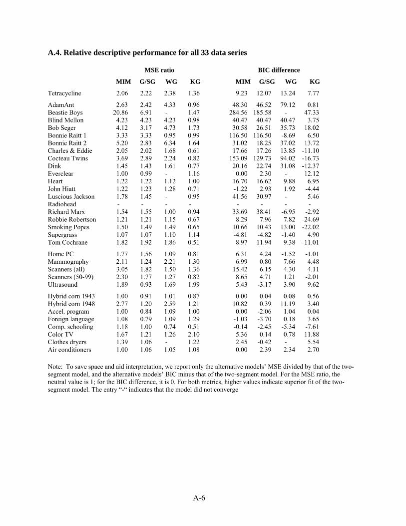
A.4. Relative descriptive performance for all 33 data series
MSE ratio BIC difference
MIM G/SG WG KG MIM G/SG WG KG
Tetracycline 2.06 2.22 2.38 1.36 9.23 12.07 13.24 7.77
AdamAnt 2.63 2.42 4.33 0.96 48.30 46.52 79.12 0.81 Beastie Boys 20.86 6.91 - 1.47 284.56 185.58 - 47.33 Blind Mellon 4.23 4.23 4.23 0.98 40.47 40.47 40.47 3.75 Bob Seger 4.12 3.17 4.73 1.73 30.58 26.51 35.73 18.02 Bonnie Raitt 1 3.33 3.33 0.95 0.99 116.50 116.50 -8.69 6.50 Bonnie Raitt 2 5.20 2.83 6.34 1.64 31.02 18.25 37.02 13.72 Charles & Eddie 2.05 2.02 1.68 0.61 17.66 17.26 13.85 -11.10 Cocteau Twins 3.69 2.89 2.24 0.82 153.09 129.73 94.02 -16.73 Dink 1.45 1.43 1.61 0.77 20.16 22.74 31.08 -12.37 Everclear 1.00 0.99 - 1.16 0.00 2.30 - 12.12 Heart 1.22 1.22 1.12 1.00 16.70 16.62 9.88 6.95 John Hiatt 1.22 1.23 1.28 0.71 -1.22 2.93 1.92 -4.44 Luscious Jackson 1.78 1.45 - 0.95 41.56 30.97 - 5.46 Radiohead - - - - - - - - Richard Marx 1.54 1.55 1.00 0.94 33.69 38.41 -6.95 -2.92 Robbie Robertson 1.21 1.21 1.15 0.67 8.29 7.96 7.82 -24.69 Smoking Popes 1.50 1.49 1.49 0.65 10.66 10.43 13.00 -22.02 Supergrass 1.07 1.07 1.10 1.14 -4.81 -4.82 -1.40 4.90 Tom Cochrane 1.82 1.92 1.86 0.51 8.97 11.94 9.38 -11.01
Home PC 1.77 1.56 1.09 0.81 6.31 4.24 -1.52 -1.01 Mammography 2.11 1.24 2.21 1.30 6.99 0.80 7.66 4.48 Scanners (all) 3.05 1.82 1.50 1.36 15.42 6.15 4.30 4.11 Scanners (50-99) 2.30 1.77 1.27 0.82 8.65 4.71 1.21 -2.01 Ultrasound 1.89 0.93 1.69 1.99 5.43 -3.17 3.90 9.62
Hybrid corn 1943 1.00 0.91 1.01 0.87 0.00 0.04 0.08 0.56 Hybrid corn 1948 2.77 1.20 2.59 1.21 10.82 0.39 11.19 3.40 Accel. program 1.00 0.84 1.09 1.00 0.00 -2.06 1.04 0.04 Foreign language 1.08 0.79 1.09 1.29 -1.03 -3.70 0.18 3.65 Comp. schooling 1.18 1.00 0.74 0.51 -0.14 -2.45 -5.34 -7.61 Color TV 1.67 1.21 1.26 2.10 5.36 0.14 0.78 11.88 Clothes dryers 1.39 1.06 - 1.22 2.45 -0.42 - 5.54 Air conditioners 1.00 1.06 1.05 1.08 0.00 2.39 2.34 2.70
Note: To save space and aid interpretation, we report only the alternative models’ MSE divided by that of the two-segment model, and the alternative models’ BIC minus that of the two-segment model. For the MSE ratio, the neutral value is 1; for the BIC difference, it is 0. For both metrics, higher values indicate superior fit of the two-segment model. The entry “-“ indicates that the model did not converge
A- 6