1

NEW SOFTWARE TOOLS FOR SIMULATIONS OF NEW INSTRUMENTS FOR THE FUTURE NEUTRON SOURCES

vorgelegt von Diplom-Physiker

Serguei Manochine aus Russland

von der Fakultät II – Mathematik und Naturwissenschaften der Technische Universität Berlin

zur Erlangung des akademischen Grades

Doktor der Naturwissenschaften - Dr.rer.nat. -

genehmigte Dissertation

Promotionsausschuss: Vorsitzender: Prof. Dr. G. von Oppen Berichter: Prof. Dr. F. Mezei Berichter: Prof. Dr. S. Hess Tag der wissenschaftliche Aussprache: 14. Juni 2005

Berlin 2005 D 83

2

3

Zusammenfassung

Neue Softwaretools für die Entwicklung von Neutronenstreuinstrumenten für zukünftige Neutronenquellen

Neutronenstreuung ist eine wichtige Technik zur Untersuchung von Struktur, Dynamik und magnetischen Eigenschaften kondensierter Materie.

Aufgrund der recht komplizierten Konstruktion und der hohen Kosten für moderne Neutronenstreu-Instrumente kann ein gewöhnlicher trial and error Ansatz zu gefährlich sein. Die Möglichkeit, die Parameter des Instruments abzuschätzen, und eine a-priori-Analyse seiner Leistungsfähigkeit erlaubt, ziemlich kostspielige Fehler zu vermeiden und die Konstruktion dahingehend zu verbessern, dass die höchstmögliche Leistung erzielt wird. Eine Möglichkeit für solche Abschätzungen und Leistungstests sind numerische Simulationsmethoden. Einen speziellen Bedarf dafür gab es durch die jahrelangen Aktivitäten am Projekt der Europäische Spallationsquelle (ESS), initiiert Mitte der neunziger Jahre. Das VITESS Programm ist am Hahn-Meitner-Institut Berlin seit 1998 entwickelt worden, insbesondere für Monte-Carlo-Simulationen von zeitlich strukturierten Neutronenstrahlen, (wie sie von Spallationsquellen erzeugt werden).

Monte-Carlo-Simulationen von Neutronenstreu-Experimenten erfordern weitere Entwicklungen zur Analyse der Leistungsfähigkeit von Instrumenten und ihrer Komponenten, auch wenn sie an kontinuierlichen Quellen - Reaktoren mit konstanter Leistung -installiert werden.

Entsprechend dieser Anforderung wurden vier neue Module (“Bender” , “Rotierendes Feld” , “Drabkin Resonator” and “Gradienten-Flipper” ) erfolgreich geschrieben, debuggt und getestet, was die Simulation der Leistungsfähigkeit von neutronenoptischen Komponenten und Instrumenten zur Streuung polarisierter Neutronen wie Spin-Echo-Instrumenten, Resonatoren und Flippern erlaubt. Die Simulation des Gravitationseffektes wurde ebenfalls erfolgreich eingebaut und getestet. Diese neuen Module bieten breite Simulationsmöglichkeiten von neuen Neutronenstreu-Instrumenten und sind inzwischen auch von anderen Programmbenutzern verwendet worden.

Vier Hauptsimulationen sind in dieser Arbeit durchgeführt worden : 1. Der konvergierende Bender für das hochauflösende Spin-Echo-Spektrometer für die ESS

wurde simuliert und optimiert. Es wurden Bedingungen für die Geometrie und das beschichtende Material gefunden, die die gewünschten Anforderungen erfüllen.

2. Das neue Kleinwinkel-Spektrometer VSANS und sein Strahlrohr mit dem multi-spektralen Extraktionssystem wurden optimiert. Die Simulationen habe gezeigt, dass ein divergenter Neutronenleiter als primäre Kollimation und das multiple Strahl-Fokussierungssystem (Viel-Loch-System) als letzte Kollimation die beste Wahl sind. Als minimaler Wert des Streuvektors wurde Qmin = 0.0033 ... 0.00067 Å-1 für einen Wellenlängenbereich von 3 bis 15 Å bestimmt.

3. Die dritte Aufgabe war es, das Neutronen-Resonanz-Spin-Echo (NRSE) Spektrometer ZETA, das am Institut Laue-Langevin in Grenoble gebaut wurde, zu simulieren und die korrekte Arbeitsweise der neuen Module zu überprüfen.

4. Der neue Typ eines Neutronen-Spin-Echo-Instruments mit dünnen magnetischen Folien (TMF) und mit rotierendem magnetischen Feld (RMF), vorgeschlagen von A. Ioffe, ist erfolgreich simuliert worden. Die Simulationen zeigten die hervorragende Leitungsfähigkeit eines solchen TMF RMF Spektrometers sowie einige nützliche und wichtige Anwendungsmöglichkeiten: „Spin Echo Resolved Grazing Incidence Scattering“ (SERGIS), „Spin Echo Small Angle Neutron Scattering“ (SESANS) und „Modulation of Intensity for Zero Effort-downstream“ (MIEZE). Die Stabilität der Spektrometer wurde bestimmt.

4

Abstract

New software tools for simulations of new instruments for the future neutron sources

Neutron scattering is an important technique for investigating the structure, dynamic and magnetic properties of condensed matters.

Because of a rather complicate construction and high cost of modern neutron scattering instruments, a usual trial and errors approach can be too risky. Therefore, a possibility to estimate parameters of the instrument and to a-priori analyse its performance allows not only to avoid quite costly mistakes, but also to improve the construction of the instrument thus achieving its best performance. A possibility for such estimations and performance tests is provided by numerical simulation methods. A special request was generated by many years activities around the European Spallation Source (ESS) project initiated in mid of 90th. The VITESS software package has been developed at Hahn-Meitner-Institute Berlin since 1998, particularly for purposes of Monte Carlo simulations with time-structured neutron beams (as they are generated by spallation sources).

However, Monte Carlo simulations of neutron scattering experiments also require further developments for the analysis of performance of instruments and/or their components to be installed at continuous sources (steady power reactors) as well.

Following this request, four new modules (“Bender” , “Rotating field” , “Drabkin resonator” and “Gradient flipper” ) were successfully written, debugged and tested allowing for simulations of performance of neutron optical components and polarised neutron scattering instruments such as neutron spin echo spectrometers, resonators and flippers. Simulation of gravity effect was successfully included and tested in the VITESS too. These new modules provide wide opportunities for simulations of new neutron scattering instruments and have been using now by other users.

Four main simulation tasks are considered in this thesis. 1. The convergent bender for the high-resolution spin echo spectrometer at the ESS was

simulated and optimised. Requirements for the geometry and coating material were found to achieve the demanded characteristics.

2. The new small angle scattering spectrometer VSANS and its beam line with the multi-spectrum extraction system were optimised. The simulations proved that the best choice is a divergent guide as the primary collimation and the multiple beam focussing system (multiple pinhole system) as the final collimation. Minimum value of the scattering vector was evaluated: Qmin = 0.0033 … 0.00067 Å-1 for wavelength range λ = 3 … 15 Å respectively.

3. The third task was to simulate the neutron resonance spin-echo (NRSE) spectrometer ZETA, which was built at Institute Laue-Langevin, Grenoble, and to check correct operation of the new modules.

4. The new kind of a neutron spin echo spectrometer with thin magnetic foils (TMF) and with rotating magnetic fields (RMF) proposed by A. Ioffe was successfully simulated. These simulations proved the perfect performance of such a TMF RMF spectrometer as well as some useful and important applications: Spin Echo Resolved Grazing Incidence Scattering (SERGIS), Spin Echo Small Angle Neutron Scattering (SESANS) and Modulation of Intensity for Zero Effort-downstream MIEZE. The robustness of the spectrometer was evaluated.

5

Table of contents 1. Introduction 7 2. About neutrons and neutron scatter ing 11 2.1 Properties and production of neutrons……………...……………….11 2.2 Wave properties of neutrons………………………………………...14 2.3 General scheme of a neutron experiment, detection of neutrons……19 3. Application of method Monte Car lo for neutron scatter ing: VITESS software package 21

3.1 Introduction…………………………………………………………..21 3.2 Main features of VITESS software package…………………………22

3.2.1 Modules in VITESS…………………………………………25 3.2.2 Modules for simulating hardware…………………………...25 3.2.3 Modules for monitoring and special modules……………….26

3.3 Module “Bender”……………………………………………………..27 3.3.1 Simulation parameters………………………..………….…..27

3.3.2 Bender geometry characteristics…………………………….28 3.3.3 Surface file………………………………………………......29

3.3.4 Reflectivity files………………………………………..…....30 3.3.5 Information file, visualisation and absorption

materials between bender channels………………………….31 3.4 Module “Rotating field”…………………………………………..….32 3.5 New features of Vitess 2.5: modules: “Drabkin resonator” and “Gradient flipper”………………………………………………………...36 3.6

Summary……………………………………………………………...…………42

4. Simulations of neutron-optics devices 43 4.1 Neutron guides and benders………………………………….………43 4.2 Convergent bender-polariser................................................................48 4.3 Simulation and optimisation of convergent benders…………..……..51 4.4 Summary………………………………………………………..……57

5. Simulations of new SANS instrument VSANS with gr id collimation 59 5.1 Introduction……………………………………………….……..……59 5.2 Simulations of the multi-spectral beam extraction system……………60 5.3 Simulations and optimisation of the primary collimation

6

of VSANS beam line………………………………………………….…..63 5.4 Final collimation system – multi-aperture pinhole collimator…………………………………………………………….…....68 5.5 Summary………………………………………………………………79

6. Neutron Spin Echo method, classical and resonance spin echo: simulations of Neutron Resonance Spin Echo spectrometer ZETA 81

6.1 Introduction……………………………………………………….…..81 6.2 Precession of the spin in a magnetic field……………………….……82 6.3 Neutron spin flipper – Mezei flipper………………………….………86 6.4 Neutron spin echo, general principal……………………………….…87 6.5 Radio frequency spin flipper……………………………………..……90 6.6 Simulations of Neutron Resonance Spin Echo spectrometer ZETA………………………………………………………..95 6.7 Summary……………………………………………………………....100

7. Simulations of Spin Echo spectrometers with rotating magnetic fields 101

7.1 Introduction……………………………………………………………101 7.2 Thin magnetic film flippers ………………………………………...…101 7.3 Propagation through the pair of TMF flippers with rotating magnetic fields. Neutron Spin Echo machine with TMF flippers………....104 7.4 Monte Carlo simulations. Application to neutron scattering instrumentation………………………………………………………….…107 7.5 Spin Echo Small Angle Neutron Scattering (SESANS) instrument…………………………………………………………..….….110 7.6 Modulation of Intensity for Zero Effort-downstream (MIEZE) instrument…………………………………………………………………115 7.7 Bootstrap configuration………………………………………...……..117 7.8 Summary………………………………………………………………120

8. Resume 121 9. Appendixes 123 References 133

7

Chapter 1

Introduction

Neutron scattering plays important roles in investigations of new materials. It provides significant and important information about position, motion of atoms and magnetic properties of solids and liquids. Neutron beams have unique properties: for example sensitivity to light elements, that can be impossible for the other kinds of beams, for example, x-ray beams. To perform these investigations, new neutron sources and instruments for scattering have been constructed and built.

Design and construction of new neutron scattering instruments is a challenging task in general. There are several main steps, which have to be performed:

1. New idea of a instrument; 2. Simple analytical calculations according to the general physical laws; 3. More detailed check of the new idea; 4. More complicated analytical calculations for finding the resolution of an

instrument – if it is possible; 5. Monte Carlo simulations of a new instrument for finding the performance

and resolution. Making the task more easily: simulations of some significant parts of a spectrometer might be made at first, later the simulations of the full instrument can be made applying conditions which are quite close to the real conditions.

If Step 4 cannot be completed, then simulations have to be made instead of

analytical calculations. The neutron is a particle without electrical charge, but possess a non-zero

magnetic moment. According to quantum mechanics, a neutron beam can be treated dually: as an ensemble of classical particles or as a wave. The treatment of a neutron as an ensemble of classical particles gives the possibility to apply the laws of classical mechanic to describe the motion of the neutron. The same applies to polarised neutron beams: then the neutron spin is considered precessing classically in a magnetic field like the spinning top. However, there is exception: the Stern-Gerlach effect cannot be treated classically. In a spectrometer the neutron behaves like a classical particle, but in a sample quantum mechanic laws have to be taken into account. All these treatments give possibilities to apply the Monte Carlo method for a simulation of new instruments.

8

The VITESS software package for the simulation of neutron scattering instruments is under development in Hahn-Meitner-Institute, Berlin since 1998 [1,2,3]. Parts of this software package are presented in the thesis. The concept, the main features and the use of the program are described with a survey of the existing modules. Particular emphasis is given to modules that are used to simulate polarised neutron and optical components, such as “Bender” , “Rotating field” , “Drabkin resonator” and “Gradient flipper” . These modules have been written by the author of this thesis. The author also included simulations of the gravity effect in the VITESS software package, especially in modules (like “spacewindow”), where it is critically necessary.

There are four main simulation tasks, which are considered in this thesis: 1) Polarised convergent benders; 2) The beam line and collimation system of the new small angle scattering

machine VSANS at Hahn-Meitner-Institute Berlin; 3) The neutron resonance spin echo machine ZETA at the Institute Laue-

Langevin, France [4] with comparison to the experimental data; 4) A new spin echo technique with rotating magnetic field and its applications;

The Soller type collimators [5] with supermirror coating [6] may be used to

polarise of neutron beams. In the case of pulsed neutron sources, the disadvantage of such devices is a high level of gamma and fast neutron background. In order to increase a neutron flux, the collimator can be made convergent. Generally, benders [5,7] make it possible to suppress the fast neutron and gamma background completely. The combination of a bender and a convergent Soller collimator (convergent or focusing bender) [8,9] can be proposed for polarisation of the neutron beam for future neutron spin-echo spectrometers at the cold source of the European spallation source (ESS) [10, 84]. Simulations and optimisation of convergent benders as neutron polarisers for NSE spectrometers are presented.

A new neutron hall has been built at the Hahn-Meitner-Institute Berlin for

initially three instruments: a new diffractometer called EXED (Extreme Environment Diffractometer) [11], a new SANS instrument called VSANS [12] and the existing Spin-Echo instrument SPAN [13]. The new beam line will serve three instruments and the existing reflectometer V6 [14] in the guide hall. The acceptance from both moderators of the multi-spectral beam extraction system [15] is explored. The simulations and optimisation of the new beam line for VSANS machine by Monte-Carlo simulations are presented as well as the “divergent guide-multi aperture” collimation system.

The neutron spin-echo (NSE) method, proposed by F. Mezei in 1972 [16], that is the most powerful tool of high-resolution neutron spectroscopy, is known in two versions: with the permanent magnetic field areas (or classical neutron spin echo [17]) and time dependent magnetic fields separated by a field free area (or neutron

9

resonance spin echo [18]). A simulations and comparison with experimental data are performed for the recently built NRSE spectrometer ZETA at Institute Laue-Langevin, Grenoble France [4].

The new version of a neutron spin echo spectrometer that makes use of spin flippers consisting of thin magnetic foils with an in-plane rotating magnetic field vector was proposed by Dr. A. Ioffe (FZ-Juelich Germany) [19]. Monte Carlo simulations are shown the perfect performance of the neutron spin echo spectrometer built with such flippers. Some important applications of this NSE technique, like Spin Echo Resolved Grazing Incidence Scattering (SERGIS) [20], Spin Echo Small Angle Neutron Scattering (SESANS) [21], Modulation of Intensity for Zero Effort-downstream MIEZE [22] are simulated as well as the robustness of the spectrometer. Requirements for thin magnetic foils are estimated. This approach can be considered as an alternative to the present-day neutron spin echo (NSE) and neutron resonance spin echo (NRSE) techniques.

10

11

Chapter 2 About neutrons and neutron scatter ing 2.1 Proper ties and production of neutrons The neutron, discovered by James Chadwick in 1932, is a sub-atomic elementary particle with zero charge but finite magnetic moment. Hence interaction of the neutron with matter is either nuclear with the nuclei of the sample, or magnetic, with the magnetic moments of the sample atoms. The basic quantities are given in table 2.1. In comparison with other elementary particles neutron is described by the absence of practically of all electrical properties: electrical charge, electrical dipole momentum and electrical polarisability. Mass 1.67492 ⋅10-27 kg Spin ½ h (h – Plank constant) Decay lifetime 887 ± 2 seconds Radius 0.7 fm Magnetic moment -9.64917⋅10-27 JT-1

Table 2.1 Basic neutron properties. It was soon understood after its discovery that the neutron is a very special, very useful particle that could provide unique and valuable insights into material properties. As sub-atomic particle, neutrons behave both as a particle and a wave. Due to the absence of electrical charge, neutrons penetrate deep into materials contrary to x-ray radiation. Neutrons interact with atoms via nuclear rather than electrical forces. Nuclear forces are very short range-of the order of a few fermis (1 fermi is 10-15 m). If there are unpaired electrons in the material, neutrons can interact by a second way: a dipole-dipole interaction between the magnetic moment of an unpaired electron and the magnetic moment of a neutron. The neutron n is an unstable particle. It decays into an electron e, a proton p

and an antineutrino_

eυ :

_

epen υ++→

12

The decay lifetime is given in Table 2.1. Free neutrons can be produced by various nuclear reactions, nuclear fission and spallation processes. Fission of the uranium isotope 235 by slow neutron capture has been the mostly frequently reaction as a neutron source as well as the Plutonium isotope 239 [86]:

MeVnfragmentstwoUn 2005.2_ 12351 ++→+

When a slow neutron interacts with a nucleus of the uranium-235 isotope, the nucleus has a certain likelihood to splitting into two fragments. The nuclear fission process releases energy and 2.5 neutrons on average i.e. for one fission 2 new neutrons, for other fission 3 new neutrons are produced. This reaction can be made self-sustaining and produce fast neutrons so that these neutrons can initiate further fission processes in the surrounding uranium nuclei, leading to a chain reaction. The reaction produces more neutrons per fission than needed to sustain this process. In this case in average 1.5 neutrons were obtained from one reaction, the rest neutron should be used to initiate a next reaction. For some isotopes (U235), the neutrons have to be thermalised before they initiate another fission process. These reactions have been realised in nuclear reactors. One of the main problems of present neutron sources is significant energy emission during the fission so complicated cooling systems are required for high-power nuclear reactors. The spectral distribution of the fission neutrons can be described quite well by a Maxwell distribution with a characteristic energy of 1.29 MeV [80]. The reaction, which was used for a first neutron source is the interaction of Beryllium with α-particles (He4). James Chadwick at Cambridge used this reaction when discovering the neutron, but very penetrating radiation was earlier observed by Bothe and Becker in 1930. But only after two years Chadwick found that this radiation is neutrons:

MeVnCHeBe 7.511249 ++→+ or (α, n) This reaction can explain that neutrons have to be nuclear constituents and electrically neutral neutrons cannot change the charge of nucleus. The neutrons possess mass and so they do change the nuclear mass. After the discovery of the neutron the reason, why nuclear masses, which are measured in units of the proton mass, are almost twice as high as nuclear charges, measured in units of the electron charge, became understandable. The part of neutrons is very significant, it is more than the half of all visible matter in the universe. There are some other reactions such as (α, n), (α, 2n), (α, pn), (p, n), (d, n) and (γ, n) that are available for producing neutron beams as well, for example:

13

114411 nNHeB +→+ or (α, n) The spallation process is a nuclear reaction where high-energy particles hit target nuclei of heavy elements [10, 84]. These high-energy particles have to have energy more than 100-200 MeV depending on the target material. The highly excited target nuclei evaporate up to 30 fast neutrons. The De Broglie wavelength of particles must be shorter than the linear dimensions of the nucleus. Collisions can also take place with individual nuclides inside the nucleus. The De Broglie wavelength λDB of a particle is given by:

mE

h

mv

h

p

hDB 2

2

===λ (2.1)

where h – Plank constant, m – mass of a particle, E – energy of a particle, p=mv – momentum of a particle with the velocity v. So the motion of any particle with momentum p can be described by a wave process with the wavelength λDB. This hypothesis was successfully confirmed by diffraction of electrons by lattices of mono-crystals; for example, American physicists Davisson and Germer using a Nickel-single crystal in 1927 [81]. Spallation processes can occur in every nucleus, although the neutron yield increases with nuclear mass. This is a significant advantage of spallation neutron sources compared nuclear fission reactors, where only a few thermally fissionable isotopes are available as is the cooling system of a target, where less energy is deposited per created free neutron. Nuclear fission reactions produce approximately six times more energy during the generation of each neutron. Particle accelerators and/or synchrotrons have been used to generate intense high-energy proton pulses directed at a target material with heavy nuclei. Examples of such sources are: ISIS in Rutherford Laboratory [82], IPNS in Argonne National Laboratory [83] and the future European Spallation Source (ESS) [10, 84]. After emission neutrons have energies of several MeV and can be transformed to thermal neutrons (energy around 0.025 eV) by collisions with light atoms [42]. This process can be called thermalisation (or cooling down) of neutrons and performed by special devices called moderators. Such cooling can be done by bringing the neutrons into thermal equilibrium with the material of a moderator. This material has to have a significant scattering cross section, for example, water or liquid hydrogen. After a few tens of collisions in the material, the energies of the neutrons become comparable to those of the moderator atoms. Thus, a moderator emits thermal neutrons from the surface with a spectrum of energies around an average value, which is determined by the moderator temperature. After cooling down in a moderator, neutrons are guided through beam lines to areas, which contain special equipment and neutron detectors: neutron spectrometers. Neutron instrumentation will be presented and explained later.

14

2.2 Wave proper ties of neutrons Despite the application of the De Broglie formula (2.1) to any particles, the diffraction processes can be only relevant for micro-particles, for example, electrons, neutrons, protons and etc. If the De Broglie wavelength of a particle is comparable with sizes of the objects, the diffraction process will take place. For particles with significant mass, the De Broglie wavelength is very small in comparison to any object. Only for micro particles such as neutron, protons and etc, the De Broglie wavelength can be comparable with the distances between the atoms of a crystal lattice. For example, if a particle with mass 0.001 kg moves with velocity 1 m/s, the De Broglie wavelength is very small: λ=0.7x10-28 cm. So diffraction can take place on objects with sizes of approximately 10-28 cm. But such objects cannot be easily observed: the atom size is already 10-12 cm. Wavelength properties play an important role for every small particle, so “diffraction of a particle at a slit” is relevant. The diffraction process means that a particle has well defined initial momentum p0 before passing a slit. After passing of the slit with size d, some deviation of the momentum ∆pX (projection of the momentum p on the axis 0X, see figure 2.1) will take place corresponding to an uncertainty of the momentum of the particle according the uncertainty principle (see later). Fig. 2.1 Diffraction of a particle with initial momentum p0 at a slit [87]. Note, that a particle has wave properties according De Broglie equation (2.1). The De Broglie wavelength λDB of a particle has to be comparable to the size of

I(x)

d

p0 Y

X

0

pX

pY

p

β

15

the slit d i.e. dDBλβ =sin . The angle β is directed to the point of the first

minimum of the diffraction process. But to obtain such a distribution I(x) experimentally, a lot of particles have to pass the slit. For the next minima of

the diffraction process: d

n DBn

λβ =sin , where n=2, 3, … This diffraction can

be easily recognized for sound in air (wavelength λ≅1 cm). For diffraction of light, special conditions are required: very small hole/holes or special devices such as diffraction gratings. But for the diffraction of x-rays (wavelength λ=10-

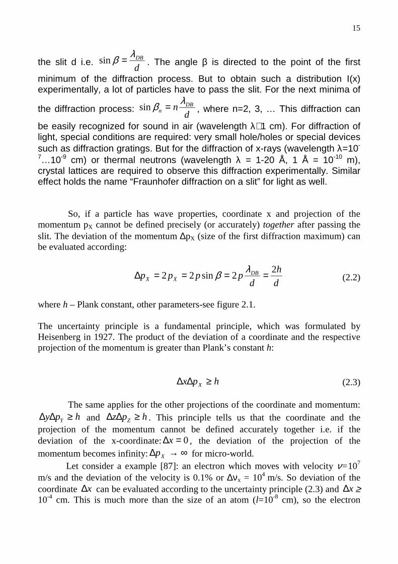
7…10-9 cm) or thermal neutrons (wavelength λ = 1-20 Å, 1 Å = 10-10 m), crystal lattices are required to observe this diffraction experimentally. Similar effect holds the name “Fraunhofer diffraction on a slit” for light as well. So, if a particle has wave properties, coordinate x and projection of the momentum pX cannot be defined precisely (or accurately) together after passing the slit. The deviation of the momentum ∆pX (size of the first diffraction maximum) can be evaluated according:

d

h

dpppp DB

XX

22sin22 ====∆ λβ (2.2)

where h – Plank constant, other parameters-see figure 2.1. The uncertainty principle is a fundamental principle, which was formulated by Heisenberg in 1927. The product of the deviation of a coordinate and the respective projection of the momentum is greater than Plank’s constant h:

hpx X ≥∆∆ (2.3) The same applies for the other projections of the coordinate and momentum:

hpy Y ≥∆∆ and hpz Z ≥∆∆ . This principle tells us that the coordinate and the projection of the momentum cannot be defined accurately together i.e. if the deviation of the x-coordinate: 0=∆x , the deviation of the projection of the momentum becomes infinity: ∞→∆ Xp for micro-world. Let consider a example [87]: an electron which moves with velocity ν=107 m/s and the deviation of the velocity is 0.1% or ∆νx = 104 m/s. So deviation of the coordinate x∆ can be evaluated according to the uncertainty principle (2.3) and x∆ ≥ 10-4 cm. This is much more than the size of an atom (l=10-8 cm), so the electron

16

position cannot be defined accurately inside an atom. However this deviation is much smaller than the size of a real instrument, for example a beam with collimating slits in an electronic microscope. So in the “macro world” deviation of the coordinate is not very important and we can use classical mechanics equations to describe the motion of electrons in electron beams. In general projections of velocities and spatial coordinates can be defined quite accurately in case of significant volumes and particles with significant masses: “macro-world” . The laws of classical physics, for example, Newton Laws and motion equations, describe this case (see chapter 3). The same formalism is applied successfully for neutron beams. Let us consider a neutron which moves with velocity ν=103 m/s. This is the velocity of thermal neutron beams with a De Broglie wavelength λ≈4 Å:

)/(

60346.395

)/(

0346.3956)(

mscmsmADB νν

λ ==

(2.4)

This formula is widely used in the VITESS software package to convert wavelengths and velocities of neutrons. The typical sizes of collimators of neutron instruments, considered later, is between 1 mm and 3 cm. The De Broglie wavelength for thermal neutrons (1-20 Å, 1 Å = 10-10 m) is much smaller, so NO significant diffraction of neutrons on collimators will take place. The neutron instrument can be treated as “macro-world” , but it is not true for crystal lattices (usual samples in neutron spectrometers), where quantum mechanical process such as the diffraction will take place. The same applies for multi aperture collimation systems as well. It should be noted, if the velocity of a particle ν is quite significant; the theory of relativity has to be taken into account (c – velocity of light), but for currently used neutron sources and beams, it is not relevant:

2

2

1

;

c

v

mvpwhere

p

hDB

−==λ (2.5)

As was mentioned before, thermal neutrons have a De Broglie λDB wavelength comparable to interatomic distances of crystal lattices and energies comparable to the collective vibration energies in condensed matter. So thermal neutrons have been successfully used to investigate structure and dynamics of condensed matter. In 1994, the Nobel Prize for physics was awarded to Shull and Brockhouse [85]. In this Nobel lecture was told: “showing where are atoms and what atoms do” .

17

To describe neutron scattering in a sample it is quite useful to work in terms of the so-called neutron wave vector k, which has magnitude k=2π/λ, where λ is the De Broglie wavelength of a neutron. This vector points along the neutron’s trajectory. So the vector k and the velocity vector v are collinear and related:

νπ

mkh =

2 (2.6)

where h – Plank constant and m – mass of the neutron. In case of elastic scattering, the wave vector is conserved in magnitude, but its direction always changes in a sample. In case of inelastic scattering, the neutron either loses energy or gains energy during the interaction: the magnitude of the wave vector changes always, but the direction may or may not change. The scattering of a neutron can be described in terms of the cross section. The cross sections σ, measured in barns (1 barn is 10-24 square cm) is equivalent to the effective area presented by the nucleus:

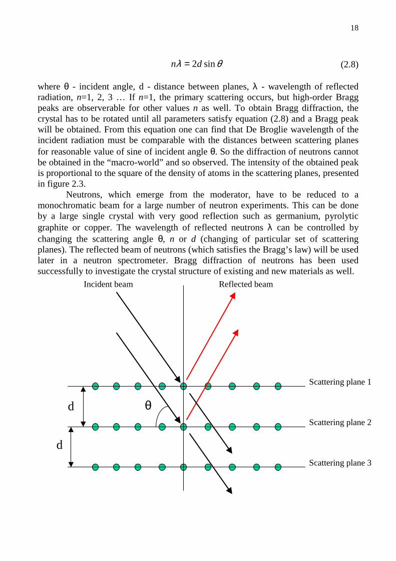
σ0II S = (2.7) where IS – number of scattering events per second (neutrons/sec) ; I0 – incident neutron flux in neutrons/cm2/sec ; σ - cross section in cm2. If a neutron hits the effective area of the nucleus, it is scattered isotropically or with similar probability in any direction. This is can be explained so: the extension of the nuclear potential is tiny compared with the wavelength of a neutron. This is not true for x-rays, because electron clouds around an atom are comparable with wavelength of the x-rays. If neutrons are scattered by matter, we need to add up the scattering from each of the individual nuclei. This is a difficult quantum-mechanical task and needs advanced calculations: analyzing of scattering from each of the individual nuclei and summarizing. But in some cases, it can be simplified significantly. The first example is elastic coherent scattering in which neutron waves interact with the whole sample such that scattering waves from different nuclei interfere with each other and can be used to explore the equilibrium structure of the sample. Inelastic coherent scattering gives information about collective motions of the atoms. William and Lawrence Bragg discovered diffraction in 1912, which received name “Bragg’s law” . This law can be understood in terms of the path-length difference between waves scattered from neighboring planes of atoms, see figure 2.3. The interference occurs between neighboring planes if the path-length difference is equal to the wavelength λ of the incident radiation (electrons, neutrons, x-rays) or multiples of λ, i.e. nλ, where n=1, 2, 3, … In this case, the neutron beam has to be treated as wave: distances between atoms are comparable with the incident wavelength. Neutron waves (or other) will effectively reflect from the crystal planes, if:

18

θλ sin2dn = (2.8)

where θ - incident angle, d - distance between planes, λ - wavelength of reflected radiation, n=1, 2, 3 … If n=1, the primary scattering occurs, but high-order Bragg peaks are observerable for other values n as well. To obtain Bragg diffraction, the crystal has to be rotated until all parameters satisfy equation (2.8) and a Bragg peak will be obtained. From this equation one can find that De Broglie wavelength of the incident radiation must be comparable with the distances between scattering planes for reasonable value of sine of incident angle θ. So the diffraction of neutrons cannot be obtained in the “macro-world” and so observed. The intensity of the obtained peak is proportional to the square of the density of atoms in the scattering planes, presented in figure 2.3. Neutrons, which emerge from the moderator, have to be reduced to a monochromatic beam for a large number of neutron experiments. This can be done by a large single crystal with very good reflection such as germanium, pyrolytic graphite or copper. The wavelength of reflected neutrons λ can be controlled by changing the scattering angle θ, n or d (changing of particular set of scattering planes). The reflected beam of neutrons (which satisfies the Bragg’s law) will be used later in a neutron spectrometer. Bragg diffraction of neutrons has been used successfully to investigate the crystal structure of existing and new materials as well.

d

d

Incident beam Reflected beam

Scattering plane 1

Scattering plane 2

Scattering plane 3

θ

19

Fig. 2.2 Bragg’s diffraction of neutrons, electrons or x-rays. The incident beam should be non-monochromatic to simplify the satisfaction of all parameters in Bragg law (2.8) during the experiments but in general a monochromatic beam is acceptable as well. 2.3 General scheme of a neutron exper iment, detection of neutrons

The combination of low flux (in comparison to x-rays sources) and weak interaction means that no common or generic instrument can be designed to explore all aspects of neutron scattering. Instead a number of instruments are available dedicate of a particular task of neutron scattering. The general scheme of a neutron experiment is presented in figure 2.3. To calibrate a neutron instrument a sample with sample environment has to be removed or standard sample (with well-known scattering properties) can be installed to find the resolution of a neutron instrument. The neutrons, which are not scattered in a sample, but are passed and reached a detector can be called “direct neutron beam” and for small angle neutron experiments the percentage of such neutrons reaches roughly 80%. For small angle neutron scattering, neutrons from the “direct neutron beam” are treated as background and have to be removed from the detection by a special device called “beam stop” . The VITESS software package has been written to simulate neutron scattering instruments starting immediately after moderators as well as some other parts of spectrometers.

NS – Neutron source, for example, a nuclear reactor or a spallation neutron source M – Moderator for thermalisation of fast neutrons P – Polariser BC – Preparation of a neutron beam, for example, monochromator, velocity selector, collimation systems and/or neutron guides. S – Sample – object being studied in an experiment A – Analyser

MNS D ABC P S

20

D – Detector or detectors with optional beam stop Fig. 2.3 General scheme of a neutron experiment [42]. Main parts of neutron spectrometer. Before and/or after sample, magnetic field volumes can be installed for a Neutron Spin Echo machine. Some of the elements are optional, for example a polariser or analyser. Neutron source and moderator are modeled according presented characteristics, i.e. total flux, wavelength band, divergences, time structure, sizes and etc. Neutrons have no electrical charge, so to detect them intermediate nuclear reactions have to be used. These reactions generate protons, γ-rays or α-particles. The three examples of such reactions [42]:

),(765.03131 pTnorMeVTpHen ++→+

),(78.43461 TnorMeVTHeLin α++→+

),(31.274101 αγγ norMeVLiHeBn +++→+

Products of the first reaction can produce ionization in helium gas detectors or generate light pulses in scintillation counters for the last two reactions. Neutron detectors can be modified to register the location at which the neutron arrived. Such detectors are called: “Position sensitive detectors” or shortly PSD detectors. A special group of neutron detectors called “ fission chambers” uses neutron capture induced fission of elements such as U235, Np237 and Pu239. These detectors can be used for monitoring neutron beams in any place mainly for testing purposes. Most of the neutrons, impinging on the chamber are not absorbed and pass through.

21

Chapter 3 Application of method Monte Car lo for neutron scatter ing: VITESS software package 3.1 Introduction Six years ago, F. Mezei organised the development of a new software package for simulations of neutron scattering instruments. It has been written at Hahn-Meitner-Institute (HMI) Berlin. It has to be well suited to simulate and check existing and new instruments at pulsed sources to support the instrumentation tasks for the planned European Spallation Source (ESS) [10]. This program was named ‘Virtual Instrumentation Tool for the ESS – VITESS’ . VITESS describes a motion of a neutron as the classical particle in the real 3-D space, excluding a sample, where neutrons have to be treated as wave. A first version was presented [1] and in 2001 the second version was released [23]. In the second version, polarisation of the neutrons and the calculation of absolute flux values were included; the program received an improved graphical user interface (GUI), see screenshot in figure 3.1. The package is available from the Internet site [24] and is free of charge under GNU license. The package supports different operational systems: Windows/DOS, Unix (SunOS: versions from 5.6, OSF1 V4.0) and Linux (kernel versions from 2.0.35). One of the main advantages of VITESS software package is that sophisticated algorithms and modules for the polarised neutron technique have been included. Some of these modules are presented in this thesis. After the first release of VITESS 1.0, the package was intensively developed. There are many spectrometers on pulsed and continuous sources were simulated: backscattering instruments [25], neutrons spin echo (NSE) instruments [26], neutron resonance spin echo instruments, see chapters 6 and 7, reflectometers [27], powder diffractometers [28], small angle neutron scattering instruments [29], etc. Triple axis spectrometers (TAS) have been simulated in comparison with other packages [30].

A new kind of neutron spin echo spectrometer with rotating fields was successfully simulated and is presented in this thesis. With the current version 2.5 – released in April 2004 - full instruments with most existing samples and devices, which are used in neutron scattering, can be checked and simulated.

Two new modules for simulating the “Resonator Drabkin” [31] and “Gradient flipper” [32] are also included in VITESS 2.5. These devices were successfully simulated and results were compared with the analytical calculations. VITESS modules successfully passed the tests and comparison with analytical calculations where it is possible.

22

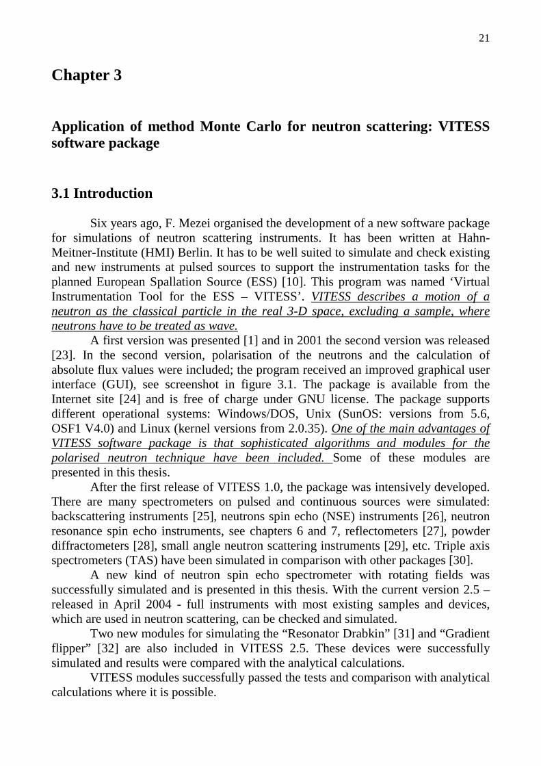
Fig. 3.1 Graphical user interface of VITESS software package, version 2.5. Example of simulations of neutron spin echo machine IN11 ZETA at the Institute Laue-Langevin, France, successfully performed by G. Zsigmond HMI [26].

3.2 Main features of VITESS software package The main concept of VITESS is that a user can run a simulation without writing any software or using any other languages. Executable programs are controlled by parameters: each component of an instrument (guide, chopper, detector, etc.) is modeled by a special module. Every module can be run at the ALL supported platforms. The simulation of a component is described by parameters and sometimes by a parameter file or files. These data can be given to VITESS via a graphical user interface (GUI) and GUI will generate a executable script with

23

modules. Alternatively, executable script can be written in any text editor. For simulation of a full instrument, a lot of modules have to be used. One module can be applied several times in a simulation. But during simulations, they all run independently. The first and very important module ‘source’ generates neutrons of certain initial properties. The neutron beam input and output represent an optionally large number of neutron trajectories each of which is described by 12 main coordinates in the following order: time of flight (TOF), wavelength, probability weight, Cartesian coordinates: (x y z), directions: (cosα cosβ cosχ), 3-component representation of the spin: (S1 S2 S3 ) [2]. A neutron propagates according the classical equations of motion:

)cos,cos,(cos

);,,(

;

;2

0

2

00

χβα⋅=

=

+=

++=

→

→

→→→

→→→→

VV

zyxr

tgVV

tgtVrr

where →→

0, rr - current and initial positions respectively; →→

0,VV - current and initial

velocities respectively; t – current time; 28.9

c

mg = and directed to the center of

earth. The 12 coordinates per neutron trajectory are consecutively written to or read from a binary file in double precision form. Some other additional parameters like neutron ID number are also included for ray-tracing purposes.

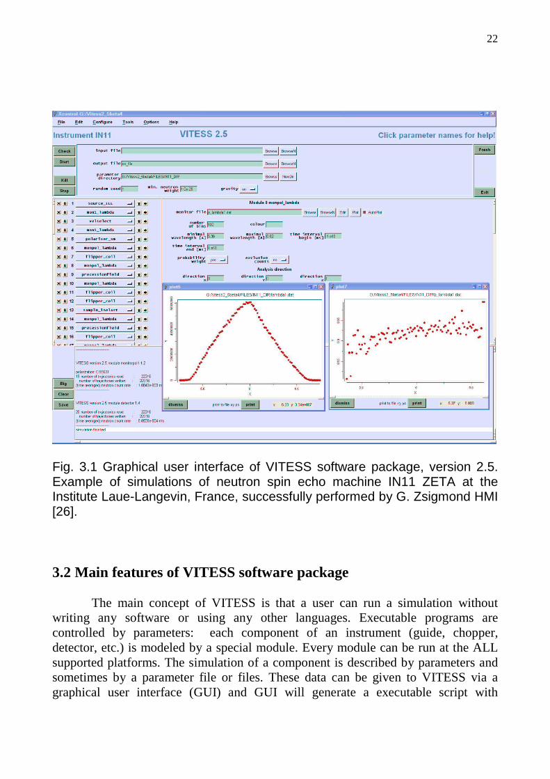
An aperture window can be installed immediately or at the some distance after the source, it is called ‘propagation window’ , see figure 3.2. This window can have some inclination relative to the source. This is very useful for simulations of real beam extracting systems: moderator-instrument. There are two moderators can be defined in the source module for simulations the multi-spectra extraction system [15].

24

Fig. 3.2 Neutron source and propagation window. Now the new values are delivered to the following module that calculates the propagation of this package to its end and so on. In a mathematical approach, each package, which is defined by random choices, represents a random event – in VITESS it is called a trajectory. The whole set of trajectories in a simulation is the random sample. Each module saves a block of 10000 trajectories (value 10000 can be changed by a user) in order to transfer the data to the next module. To avoid a need of large memories for intermediate results, the second module is started immediately after the data are transferred. The same is valid for all other modules in the simulation. In principle, all modules may run at the time in simulations. This is the concept of piping, which is suitable for DOS (WINDOWS) and UNIX (Linux) operations systems [33]. Simulations can be divided into two or more parts at any point of the instrument. As an example, the primary part of the spectrometer can be simulated only once and all data are saved in a binary file instead of delivering them to the next module. This file is treated as a “virtual source” . Now the second part of the spectrometer reads the binary file as input and simulations can be continued with a virtual source. This second part needs by far less time than the first part. If the instrument parameters variations of interest are only in the second part, this approach can save a lot of computing time. But this trick can be useful, if time of simulations of the second part is quite short in comparison with the first part of an instrument. In the source module, a count rate is calculated for each trajectory depending on wavelength, number of trajectories, etc. This count rate can be changed by reflections, absorption inside material, etc. If a trajectory does not hit any component or the count rate is below the ‘minimal weight’ , it is deleted from the simulations: the neutron is died. A user has to choose the ‘Minimal weight’ . The sum of all trajectories gives the “neutron current” calculated after each module. The user has to calculate flux values at moderators himself or measure it.

25

Apart from the properties already described (position, time of flight, direction, and count rate), a spin-state (in 3-dimensional representation) is generated for each trajectory and the spin-orientation is calculated during its flight through the instrument. Several modules have been written to simulate instruments with polarised neutrons, i.e. modules for polarisers, static and dynamic precession fields, flippers and polarimeters. Every trajectory is identified by a parameter, which is called ID. This gives possibilities for ray tracing of trajectories. For all trajectories, whose ID is found in an input file, all parameters at beginning and end of each module are written to files. Alternatively, the module ‘writeout’ can be used to see the whole data set, transferred from one module to the following. In the last versions, some tools were included to make the creation of input data much easier and/or to process output data. Ray tracing can be useful for checking the acceptance of a moderator-instrument beam extraction system. Acceptance means which part of the neutron flux is accepted by a first component of a spectrometer, usually by a neutron guide. This is usually depended from the wavelength of neutrons. 3.2.1 Modules in VITESS There are two kinds of modules in the VITESS software package. The first type simulates hardware devices of neutron spectrometers. The second type is used to visualise, and/or to evaluate or write data. 3.2.2 Modules for simulating hardware VITESS modules can simulate a lot of devices used in a neutron scattering instrument. These are basic components like source, guide, windows (or apertures), choppers, detectors, several samples and numerous modules for polarised neutron technique. Figure 3.3 gives a full list of modules. Some of the modules can be used to simulate optical devices; these are ‘supermirror-ensemble’ , ‘bender’ , and ‘guide’ . The module ‘elliptic mirror’ simulates an elliptically shaped surface. Modules for simulating polarised neutron beams are also available now.

26

Fig. 3.3 VITESS modules for simulating hardware. 3.2.3 Modules for monitor ing and special modules There are several modules available for monitoring of the intensity as a function of one or two parameters. Such parameter can be wavelength, time, divergence into one direction etc. These modules are just compressing data by a binning procedure. The number of bins and their size have to be given by the user. The polarisation as a function of any parameter at the chosen direction can be calculated by a special kind of monitor modules. Such a system is called a “neutron polarimeter” or in our case “ ideal polarimeter” . Additionally, there are two modules available to do a bit of data evaluation: ‘Eval_elast’ and ‘Eval_inelast’ . They calculate intensity as a function of a parameter that is not directly used in the simulation, e.g. the d-spacing for diffraction. The module ‘ visualise’ shows the trajectories hitting a plane during the run. This module is very useful for testing instrument geometry and correctness of simulations. The module ‘writeout’ writes the full data set into a file. This has also been used for a ray-tracing option. The ‘ frame’ module changes the co-ordinate system of the trajectories. Mirroring, translation, rotation or combination of them can be performed. This is effectively a change in the instrument (in the opposite direction). It

! "

!

# $

# $

$ % "

& ! !

" "

#

# $

#

' #

(

)

*

#

+ , !

!

-

' $

$ !

. / )

.

- % "

$

27

can be used to simulate components that are different from the geometry assumed in the module, e.g. benders curved to the right instead of curved to the left (as realized in the bender module). But this module has to be used carefully. The changing of all coordinates will change a configuration of the spectrometer with neutron trajectories, but not ONLY neutron trajectories. So framing CANNOT be used as “some kind of ideal elastic neutron scatter” . 3.3 Module “ Bender ” The module “Bender” is similar to the module “Guide” using the bender option. The main difference is that the 'bended guide' consists of several straight parts that form a polygon section. In contrast, the bender surfaces are cylinder surfaces (see figure 3.2), but straight planes are also possible. This module also simulates converging or diverging bender-polariser with the possibility of enabling or disabling the polarisation of neutrons. The 2-D visualisation of surfaces to check the layout of the bender and to trace the neutron paths is included. Only the first 10000 trajectories will be visualised. Also the device for visualisation can be chosen: display, file or both of them. If device is display, you will see a visualisation at a screen. If device is file, a postscript file will be generated and can be visualised later. Additionally there is a possibility to have spacing inside the bender: bender walls have thickness in cm. A cross talk between channels is treated as well as absorption inside the channels or in the material dividing the channels. Several hundred surfaces (300) can be defined. Positions at the beginning and at the end as well as the curvature can be defined for each plane. This information is saved in a file. With this concept, a broad variety of benders can be simulated – normal benders as well as polarising benders and solid-state benders; channels may have converging or diverging channels or spacing in the beginning or at the end. But even an extraction system with plane mirrors and couple moderators has been simulated by means of the “Bender” module. This extraction system was simulated by means of the “Sm_ensemble” module too. No significant difference has been found. Figure 3.4 shows an example of bender surface visualisation. 3.3.1 Simulation parameters

The full list of parameters (options) can be found in the appendix I. The effect of gravity is considered in this module, if no cylindrical surfaces of the bender are used. Neutrons with a probability/current less than the 'minimal weight' are taken out of the simulation. The roughness of a reflecting surface of a bender is included too. The abutment loss feature rejects neutrons, which have got reflection near the edges (exit) of the bender [34]. If the last path of a neutron (before the exit plane) is smaller than a given value, such a trajectory is rejected. The user can choose this value or disable the option. The polarisation of neutrons may be enabled or disabled. For each spin direction (spin up or spin down), the user has put individual reflectivity files for

28

left, right and top/bottom planes of the bender, totally six files (This can not be actually for top and bottom planes, but it is possible) too. If polarisation is included, neutrons, which have the other quantisation direction, are rejected.

Fig. 3.4 Visualisation of a bender channels.

3.3.2 Bender geometry character istics The general geometry of a bender is defined by the four main parameters:

a) Entrance height (along vertical axis 0Z). b) Exit height (along vertical axis 0Z). c) Length of the bender - L. d) Radius of curvature - Rc.

29

The angle β defines the angle of the declination of the exit surface relative to the entrance surface of the bender; so the bender axis is a part of a circle. The angle β is calculated by the formula:

cR

L=β (3.1)

If the radius of curvature is inputted as zero in the module, the central axis of the bender is a straight line and so the angle β is zero too. Such a bender has no curvature.

The parameters that describe the arrangement of vertical surfaces in the horizontal plane (XY - plane) are read from a parameter file, which has the name – “surface file” .

3.3.3 Sur face file

The entrance and exit position of each surface and its radius have to be given in a surface file. All benders that can be described in that way might be simulated. The surface file has to be written by the user and to put in with the option -u. The surface file contains rows and THREE columns. Each row describes the respective surface of a bender and consists of three columns: displacement at the entrance surface, displacement at the exit surface, radius of curvature. An example of the surface file with eleven surfaces is presented in the table 3.1.

-10.0 -5.0 2000.0 -8.0 -4.0 2000.0 -6.0 -3.0 2000.0 -4.0 -2.0 2000.0 -2.0 -1.0 2000.0 0.0 0.0 2000.0 2.0 1.0 2000.0 4.0 2.0 2000.0 6.0 3.0 2000.0 8.0 4.0 2000.0 10.0 5.0 2000.0

Table 3.1 Example of the surface file. This bender is visualised in figure 3.4. All values are cm.

For a positive value of the radius of curvature the arch will have a concave

shape, see figure 3.4 as example. If the radius of curvature of a surface is given as zero, a straight line (planes) will be used instead, so no curvature exists. This is useful for simulations of Soller collimators. If a negative value of the radius of curvature is given, the arch will have a convex shape. Such features give the possibilities for

30

simulating many types of benders and collimators! The module calculates the number of lines in the surface file automatically.

3.3.4 Reflectivity files

The reflectivity files describe the reflection properties of the coating. The files, which describe the reflectivity can be found in the VITESS directory FILES [24]:

a) mirr0.dat: absorbing coating (no reflectivity) b) mirr1a.dat: Ni coating (θNi = 0.099138 degree for wavelength 1 Å or m=1) c) mirr1b.dat: θNi58 coating (θNi = 0.11456 degree for wavelength 1 Å) d) mirr2.dat: super-mirror coating (2θNi or m=2) e) mirr2linear.dat: supermirror coating,

The reflectivity file contains the probability of reflection in dependence of the incident angle for neutrons with a wavelength of 1 Å. Each row contains 10 data points and covers 0.01 degree, i.e. each point gives the probability average over an angular interval of 0.001 degree (the second row covers 0.01-0.02 degree and so on.). The number of data points may vary between 1 and 1000. If the end of file is reached (e.g. only 52 values are given) the probability to reflect 1 Å neutrons for higher angles is set to zero or no reflectivity. If no reflectivity file is given as an input or mirr0.dat file is given, the guide operates in total absorption mode, i.e. each neutron hitting a guide wall is lost or transmitted in the next channel (depending on mode). The reflectivity values have to be obtained experimentally or by analytical calculations.

The reflectivity file mirr1a.dat which is describes natural nickel (Ni) is presented:

0.99 0.99 0.99 0.99 0.99 0.99 0.99 0.99 0.99 0.99 0.99 0.99 0.99 0.99 0.99 0.99 0.99 0.99 0.99 0.99 0.99 0.99 0.99 0.99 0.99 0.99 0.99 0.99 0.99 0.99 0.99 0.99 0.99 0.99 0.99 0.99 0.99 0.99 0.99 0.99 0.99 0.99 0.99 0.99 0.99 0.99 0.99 0.99 0.99 0.99 0.99 0.99 0.99 0.99 0.99 0.99 0.99 0.99 0.99 0.99 0.99 0.99 0.99 0.99 0.99 0.99 0.99 0.99 0.99 0.99 0.99 0.99 0.99 0.99 0.99 0.99 0.99 0.99 0.99 0.99 0.99 0.99 0.99 0.99 0.99 0.99 0.99 0.99 0.99 0.99

0.99 0.99 0.99 0.99 0.99 0.99 0.99 0.99 0.99 0.00 0.0

31

3.3.5 Information file, visualisation and absorption mater ials between bender channels The information file is generated after the run of simulations and contains full information about the bender geometry. This information can be useful, if the bender will be built. For simulations, it is not necessary.

The visualisation of the bender, which is described in the above-mentioned file (see table 3.1), is given in figure 3.4. The other parameters of the bender: length is 2 m, radius of curvature is 20 m, and thickness of surfaces is neglected. During simulations, the neutron flight paths will appear. After first reflection, the color of the neutron path changes, so this gives the possibility to check absence of a background of fast neutrons and/or "straight line of sight" gamma rays. For UNIX operation systems such as Linux, SunOS, Solaris, OSF1 the PGPLOT graphic library is used. For Windows operation system the PGPLOT [35] and G2 [36] graphics libraries are used together. In chapter 4, a visualisation of a bender with neutron paths is presented.

Some absorption materials were included in the module Bender. It allows to use them without looking for material properties. These materials have to be used between bender channels to prevent cross talk of neutrons between channels.

a) Read data from a file, which has created by a user b) Gd: Gadolinium c) Cd: Cadmium d) B10 e) Eu f) Si: Silicon. g) Vacuum, no attenuation, not suitable for bender

For gadolinium, cadmium, B10 and Eu the wavelength range has to be between

0.3 and 28 Å in the source module or virtual source. The wavelength range should not be broad after any kind of a monochromatisation system. For Silicon the wavelength range has to be between 1 and 20 Å in the source module or virtual source. Otherwise, the simulation process will be canceled automatically with error messages. Thomas Krist, HMI gave these data. The transmission Trans is calculated by the formula:

)( DeTrans ⋅−= µ (3.2)

where µ is characteristic of a material and depends on the wavelength of a neutron. D is the distance, which is passed in this material by a neutron.

32

3.4 Module “ Rotating field”

A special module developed for the VITESS software package allows to perform Monte Carlo simulations of the neutron spin behavior in time-dependent magnetic fields – rotating fields, see figure 3.5. The first version of the module was included in VITESS 2.3. In this module the rotating magnetic field region is considered to consist of a number of layers with stepwise change of the magnetic field direction and/or magnitude. The thickness of these layers has to be selected to be sufficiently small to consider the magnetic field as stationary on the time scale of neutron propagation through any individual layer, see figure 3.6. This is can be done experimentally: for the first simulation, we have to choose N layers; for the second simulation 2*N layers have to given. Then, both results are compared. If no significant differences were found, the initial number of layers N is acceptable for such conditions.

Using the equation of spin motion in the stationary magnetic field, the subroutine consequently calculates the components of the neutron spin after propagation through the n-th thin layer and uses these components as input for the calculations to be performed for the (n +1)-th layer. Saying by other words, we are performing the numerical integration of the Bloch equation (6.2). The magnetic field rotates around one axis: OX or OY or OZ. A permanent magnetic field can be added to the rotating field. This is useful for simulations of radio frequency (RF) flippers and thus for neutron resonance spin echo (NRSE) instruments. A random magnetic field can be added too. Rotating magnetic field can be excluded from simulations so only permanent magnetic field components will be considered for the precession. This can be useful for simulations of a classical neutron spin echo machine or a combination of the NSE and NRSE spectrometers.

The spin precessions are treated classically i.e. this module only rotates the spin vectors belonging to trajectories, which pass through the rectangular geometry according the applied magnetic field. No attenuation of the neutron count rate is considered during the flight.

33

Fig. 3.5 Rotating and permanent magnetic fields configuration. Small green arrow is direction of rotation of a magnetic field.

Rotating field

Permanent field components

Y

X

Z

Direction of neutron flight

Coordinate system

0

34

Fig. 3.6 Dividing the precession volume into a number of layers. Blue arrows are current directions of a rotating magnetic field. Dependence of the final spin position on the number of slices N.

The BOOTSTRAP [37; chapters 6, 7] option can be activated. In this case the precession volume is divided for two parts. For the first part the frequency of a rotating field and all permanent components are chosen as input dates. For the second part all these parameters are become negative: multipled by -1.0 value. Negative frequency means the opposite direction of rotation of a rotating magnetic field.

=

35

ROTATING FIELD WITH PERMANENT MAGNETIC FIELD

FORMULAS OF ROTATION: AROUND AXIS 0X

X = X0 (3.3) Y = Y0 + FieldValue*sin(Ω* (T + TOF) + BeginPhase) (3.4) Z = Z0 + FieldValue*cos(Ω* (T + TOF) + BeginPhase) (3.5)

FORMULAS OF ROTATION: AROUND AXIS 0Y

X = X0 + FieldValue*sin(Ω* (T + TOF) + BeginPhase) (3.6) Y = Y0 (3.7)

Z = Z0 + FieldValue*cos(Ω* (T + TOF) + BeginPhase) (3.8)

FORMULAS OF ROTATION: AROUND AXIS 0Z

X = X0 + FieldValue*cos(Ω* (T + TOF) + BeginPhase) (3.9) Y = Y0 + FieldValue*sin(Ω* (T + TOF) + BeginPhase) (3.10)

Z = Z0 (3.11)

where T is local time, X0, Y0, Z0 are the components of the permanent magnetic field, Ω is angular frequency, FieldValue is strength (amplitude) of the rotating magnetic field, TOF is time of flight of neutron from preceding modules for phase of a rotating field. If TOF is equal zero, the magnetic field is directed vertically upwards for the rotation about the axis 0X, when NEUTRON HAS LEFT THE MODERATOR SURFACE and the rotation of the magnetic field and neutron time of flight are NOT SYNHRONISED and such a case cannot be suitable for the Resonance Spin Echo simulation.

The amplitude FieldValue can have five types of distributions:

a) Normal_ran: Normal randomisation of amplitude during the domains changing.

b) Uniform_ran: Uniform randomisation of amplitude during the domains changing.

c) Normal: Normal distribution of FieldValue with the amplitude FieldValue. d) Uniform: Permanent value FieldValue. e) From_file: Distribution is read from a file, which a user has created.

36

The last possibility is very useful for simulating a realistic magnetic field, for example a magnetic field of a solenoid. The frequency of rotation and the components of the permanent magnetic fields can be randomised. The calculated amplitude of the rotating field can be found in the VITESS output window and will be used as the parameter "amplitude of the rotating magnetic field". Randomisation means that, new random value (for example “Amplitude of the rotating field” ) will be generated randomly after passing in a next layer.

This module has been successfully used for simulations of the performance of realistic rotating magnetic fields of neutron spin echo spectrometers (NSE-RMF) and its applications for inelastic neutron scattering. The final realisation has been included in VITESS version 2.5. See the appendix I for the full list of options for the module.

3.5 New features of Vitess 2.5: modules “ Drabkin resonator ” and “ Gradient flipper” This version 2.5 contains two new modules to simulate instruments with polarised neutrons: “Drabkin resonator” [31] and “Gradient flipper” [32, 38]. See the appendix I for the full list of options for the modules. The general concept of these modules is the same as in the module “Rotating field” .

Direction of neutron flight

Coordinate system Z

X

Y

0

static guide magnetic field Final polarisation

Pz=-1for resonance wavelength

Initial polarisation Pz=1

periodical magnetic field

37

Fig. 3.7 Drabkin resonator. General scheme.

The first module ‘Drabkin resonator’ can be used to simulate a Drabkin resonator system. This system has to have two magnetic fields, see figure 3.7. The main field is a periodical magnetic field with permanent amplitude or with some amplitude distribution. The permanent magnetic field has to be added into the periodic magnetic field. This field is called “guide magnetic field” and has to be oriented perpendicular to the periodical magnetic field. If we apply these two fields, we will receive a flipper, which works in a narrow wavelength range. This can be explained by the resonance condition of a spin as well as in a radio-frequency (RF) flipper, see chapter 6. The amplitude distribution of the periodical field can have a gauss or sinus law. This gives the possibility to improve the final polarisation distribution Pz(λ) of neutrons, which was flipped: remove the high harmonics, see figure 3.8. The full width on the half height of the received peak depends on the number of periods of the periodical magnetic field. The incoming neutron beam should contain some wavelength range. No monochromator should be installed before the resonator. A random magnetic field can be added also to simulate real magnetic field configurations. In this module, the spin precessions are treated classically i.e. this module only rotates the spin vectors belonging to trajectories, which pass through the rectangular geometry. No attenuation of the neutron flux is considered during the flight. An example of simulations of the “Drabkin resonator” is given at the figure 3.8. The initial polarization is PX=0, PY=0, PZ=1. This flipper has the following parameters: Dimensions of the field volume are X=20 cm (length), Y=10 cm and Z=10 cm. Number of periods is 100 or 200 layers. The amplitude of the periodical magnetic field is 1.33 Oe for uniform amplitude distribution. The amplitude of the periodical magnetic field is 2.1 Oe for sinus amplitude distribution. The guide magnetic field is 170 Oe for both cases. The resonance wavelength is around 4 Å.

38

3.85 3.90 3.95 4.00 4.05 4.10 4.15-1.0

-0.5

0.0

0.5

1.0

1.5

Pol

aris

atio

n, P

z

Wavelength, Ang.

Sinus distribution of amplitude of the periodical magnetic field Uniform distribution of amplitude of the periodical magnetic field

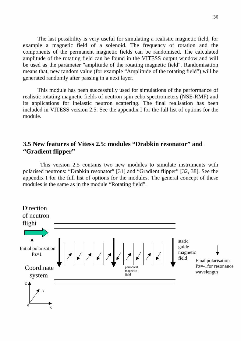
Fig. 3.8 Simulations of the “Drabkin resonator” for two kinds of amplitude distribution of the periodical magnetic field: final distribution Pz(λ). Initial polarisation of a incident beam is Pz=1. Final polarisation is –1 only for the resonance wavelength ≈4 Å. The module ‘gradient flipper’ [32] simulates a flipper, in which the spin follows a magnetic field adiabatically. In this way it is possible to flip neutrons of a “white” beam, for example in a time of flight instrument. This module simulates spin precessions in the magnetic field of a special kind, see figure 3.9. This flipper was described in ref. [38].

39

Fig. 3.9 Gradient flipper: field configurations. Initial spin position is parallel to the axis OZ and directed vertically upward.

The first part of such a field is a rotating magnetic field. The amplitude of this field has to be changed by sinus function with a semi-period, which is equal to the appropriate dimensions of the rotating field volume. The magnetic field has to be rotated around the axis OX or OY or OZ. The axis OX has the direction of the neutron flight. A permanent value of the amplitude can be given too. The second part of the general field is a guide magnetic field. The spin precessions are treated classically, i.e. this module only rotates the spin vectors belonging to trajectories which pass through the rectangular geometry. A random magnetic field can be added. No attenuation of the neutron beam is considered during the flight. The formulas, which describe the rotating fields are the same as for the module ‘Rotating Field’ , see formulas (3.3)…(3.11). But for a gradient flipper, the amplitude FieldValue of the rotating magnetic field has to have sinus law with semi-period - appropriate dimensions of the magnetic field volume. A permanent amplitude FieldValue is not acceptable for a gradient flipper, but included in the module for debugging purposes. The guide magnetic field can have three types of distribution:

a) Cosine law: with semi-period - appropriate dimensions of the magnetic field volume, acceptable for a gradient flipper;

b) Linear law: with period - appropriate dimensions of the rotating field volume, best solution and realised for a gradient flipper;

c) Permanent law, not acceptable for a gradient flipper;

Static field Static field RF-field

Y

X

Z

Direction of neutronflight

Coordinate system

0

Two rotating fields

RF-field Two counter rotating fields

40

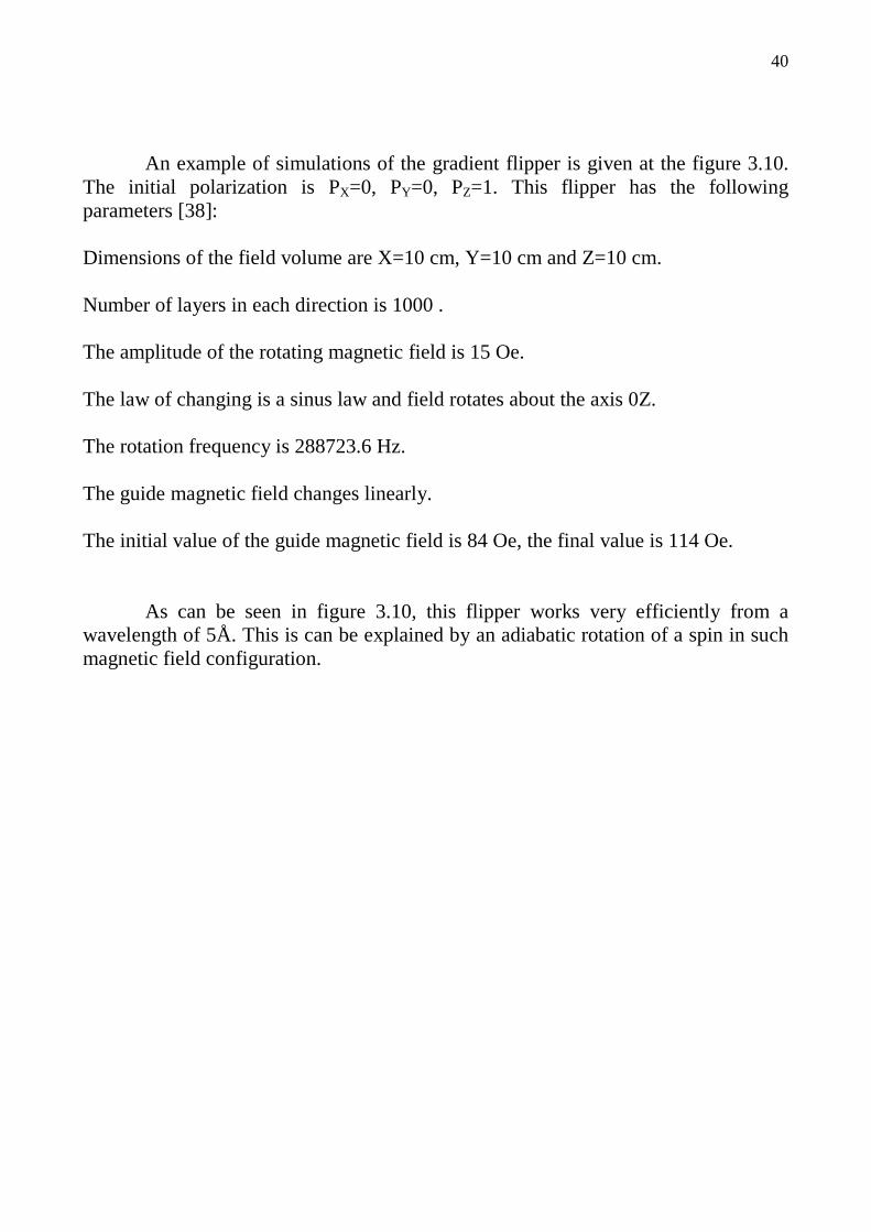
An example of simulations of the gradient flipper is given at the figure 3.10. The initial polarization is PX=0, PY=0, PZ=1. This flipper has the following parameters [38]: Dimensions of the field volume are X=10 cm, Y=10 cm and Z=10 cm. Number of layers in each direction is 1000 . The amplitude of the rotating magnetic field is 15 Oe. The law of changing is a sinus law and field rotates about the axis 0Z. The rotation frequency is 288723.6 Hz. The guide magnetic field changes linearly. The initial value of the guide magnetic field is 84 Oe, the final value is 114 Oe. As can be seen in figure 3.10, this flipper works very efficiently from a wavelength of 5Å. This is can be explained by an adiabatic rotation of a spin in such magnetic field configuration.

41

2 4 6 8 10 12 14 16 18 20-1.00

-0.75

-0.50

-0.25

0.00

0.25

0.50

0.75

1.00P

olar

isat

ion

Pz

Wavelength, Angst.

Initial polarisation Pz=1 Final polarisation after flipper

Fig. 3.10. Flipping of a polarised neutron beam by the gradient flipper: final distribution Pz(λ). Initial polarisation of an incident beam is Pz=1.

42

2.6 Summary In this chapter I described a general introduction in the VITESS software package. There are four significant modules available now: “Bender” , “Rotating field” , “Drabkin resonator” and “Gradient flipper” . The author developed these modules individually. I also participated in development of such modules:

1) Module “guide” . 2) Module “grid” . 3) Module “elliptical mirror” . 4) Module “visualisation” 5) Option for simulating gravity for whole VITESS. All these modules have been tested and used for different kinds of

simulations. Some of them are presented in this thesis.

43

Chapter 4

Simulations of neutron-optics devices 4.1 Neutron guides and benders

A neutron guide is a tube with a squared or circular cross section. The tube can be straight or curved (see figure 4.1).

Fig. 4.1 Neutron guide, general example.

There are other kinds of combinations of tubes that can be constructed. The walls of a neutron guide have to be reflecting for neutrons at least for a desirable wavelength range of a neutron beam. E. Fermi made the basic invention in 1946. He found that neutrons could reflect from solid materials, they were called neutron mirrors. In 1960 B. Alefield built the first neutron guide. Each reflecting material is described by an important parameter: the cr itical angle [39]. The critical angle cγ is the maximal angle, for which neutrons can still be fully reflected from a material.

The critical angle is defined by the refraction coefficient n of a material versus vacuum:

44

.cos nc =γ (4.1) The critical angle is quite small for cold and thermal neutrons and so γγ ≈sin for the γ ≤ 15°.

.1 22 nc −=γ (4.2)

For an ideal mirror surface, the reflection coefficient is 1, for angles less than the critical angle and for other angles it can be calculated by the formula [40].

.sin))(cos(

sin))(cos(2

2/122

2/122

+−−−=

γγγγ

n

nR (4.3)

For small angles γ it can be rewritten as:

.)/1(1

)/1(12

2/122

2/122

−+−−=

γγγγ

c

cR (4.4)

The critical angle of a material is calculated by the formula [41]:

.π

λγ cc

Na= (4.5)

where λ - wavelength in Å, ca - coherent amplitude of scattering in Å, N – nuclear

density in 3−

A of material. This formula can be obtained from energy conservation law, when neutron is entering into the medium from vacuum [42]:

.2/2/ 220 UmVmV += (4.6)

Where V0 – velocity of neutron in vacuum, m – mass of neutron, V – velocity of

neutron in medium and U potentional energy of neutron in a medium (h – Planck constant):

cNam

hU

22π= (4.7)

Refraction coefficient n defined similar as in optic:

0V

Vn = (4.8)

There are a several basic reflection materials available. They can be found in table 4.1. The critical angle of natural Ni usually is accepted as basic characteristic and called “m=1” . Recently the supermirrors were developed and developing still

45

today. They have 2 to 5 times a critical angle of usual Ni. If the critical angle of a supermirror is 0.0034 rad., we can call it “m=2” . Material Critical angle cγ [rad] for 1 Å Glass 0.0011 Cu 0.0014 Ni (natural) 0.0017 (“m=1”) Ni58 0.0020

Table 4.1 Basic reflecting materials [39].

Neutron guides or benders can polarise a neutron beam by reflection, if the medium is magnetised in a given direction. The refraction coefficients n+ and n- are different for each neutron with parallel and anti-parallel spin orientations (spin-up and spin-down) [42]:

),)(2/(1 2 µπλ CaNn c +−=+ (4.9)

),)(2/(1 2 µπλ CaNn c −−=− (4.10)

where areλ - wavelength in Å, ca - coherent amplitude of scattering in Å, N –

nuclear density in 3−

A of material, C=0.265x10-12cm/µ,B (µ,B- Boron magneton), µ - magnetic moment of the atom.

So applying the magnetic field to a mirror, we will have two different reflections, depending on the spin orientation. The parameters can be chosen in such a way that one refraction coefficient is comparable with supermirror m=2 and second refraction coefficient is comparable with m=0.5 [43]. In other words, after reflection we will have a polarised neutron beam or neutron polariser. But the intensity of the neutron beam will be decreased by a factor of 2. There are a lot of different materials available today for polarisation with the first refraction coefficient m>2 and the second refraction coefficient m < 0.5 [38, 44].

The reflecting neutron guides are often used to shift the effective source of an instrument to a distance away from the moderator. Such movement can allow the instrument to be situated in a region with low background. To decrease the background of fast neutrons and gamma rays a curved neutron guide has to be used at pulsed neutron sources. It is used to prevent the so-called “direct line of sight” .

The angular divergence of neutrons at the exit of a guide is determined by the critical angle and is not dependent on the angular divergence of neutrons at the entrance of the neutron guide. The neutron guide can accept only a quite narrow range of angles and wavelength. At the exit a neutron guide delivers a significant percentage of neutrons. For example a straight neutron guide with a length of 100 m can deliver around 40% of all accepted neutron beam.

46

A curved neutron guide with a = 3 cm and a characteristic wavelength of 10 Å has a radius of curvature R = 200 m and must be at least 3.5 m long to prevent “direct line of sight” and guides with shorter characteristic wavelength have to be even longer [5]. Time of flight (TOF) instruments have to be short to avoid the frame-overlap problems.

The neutrons in the each pulse begin their flight to a detector at practically the same time: within a small fraction of milliseconds. But they all have different energies or velocities, as time passes they spread out along the course, reaching the same distance from the moderator at different times after departure. So fast neutrons from a current pulse can reach a detector in the same time as slow neutrons from the previous pulse: wavelengths of neutrons can be mixed during the analysis. Such effect is called “Frame overlap” . Frame overlap problems are actually for a time of flight spectrometer with significant length at pulsed neutron sources with a high frequency of impulses.

One of way of overcoming this length problem is to use a beam bender [45], which is effect an array of short narrow curved guides.

The neutron bender is a curved multislit neutron guide, see figure 4.2. Using natural nickel coated bender with a radius of curvature of 25 m, the slit width is of an order of 1 mm, over a length of about 45 cm it is possible to remove fast neutrons and γ-rays from the neutron beam [5]. Beam benders of a length of 1 m or even less have been designed and built to move the detector out of the line of the direct beam.

R – radius of curvature

L - length

Direction of flight

H - height

V

d

channels

47

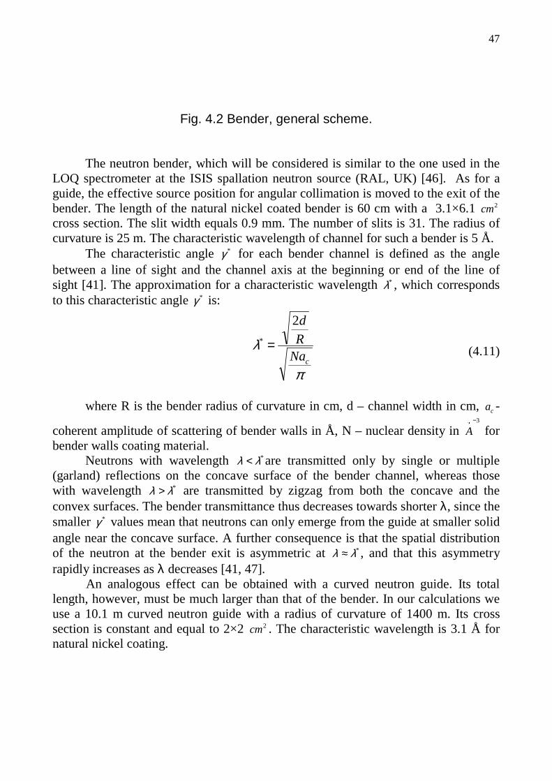
Fig. 4.2 Bender, general scheme. The neutron bender, which will be considered is similar to the one used in the

LOQ spectrometer at the ISIS spallation neutron source (RAL, UK) [46]. As for a guide, the effective source position for angular collimation is moved to the exit of the bender. The length of the natural nickel coated bender is 60 cm with a 3.1×6.1 2cm cross section. The slit width equals 0.9 mm. The number of slits is 31. The radius of curvature is 25 m. The characteristic wavelength of channel for such a bender is 5 Å.

The characteristic angle *γ for each bender channel is defined as the angle between a line of sight and the channel axis at the beginning or end of the line of sight [41]. The approximation for a characteristic wavelength *λ , which corresponds to this characteristic angle *γ is:

π

λcNa

R

d2* = (4.11)

where R is the bender radius of curvature in cm, d – channel width in cm, ca -

coherent amplitude of scattering of bender walls in Å, N – nuclear density in 3−

A for bender walls coating material.

Neutrons with wavelength *λλ < are transmitted only by single or multiple (garland) reflections on the concave surface of the bender channel, whereas those with wavelength *λλ > are transmitted by zigzag from both the concave and the convex surfaces. The bender transmittance thus decreases towards shorter λ, since the smaller *γ values mean that neutrons can only emerge from the guide at smaller solid angle near the concave surface. A further consequence is that the spatial distribution of the neutron at the bender exit is asymmetric at *λλ ≈ , and that this asymmetry rapidly increases as λ decreases [41, 47]. An analogous effect can be obtained with a curved neutron guide. Its total length, however, must be much larger than that of the bender. In our calculations we use a 10.1 m curved neutron guide with a radius of curvature of 1400 m. Its cross section is constant and equal to 2×2 2cm . The characteristic wavelength is 3.1 Å for natural nickel coating.

48

Benders or the curved neutron guides allow to suppress completely the fast neutron and gamma backgrounds from reactors or spallation neutron sources.

A comparison of transmission coefficients of the neutron bender with natural nickel coating and supermirror coating (m=2, λγ 0034.0=c (Å)) and a natural nickel-coated neutron guide is shown in figure 4.3. It is seen that the best results are obtained for the bender with a supermirror coating but only for short wavelengths. The supermirror coated neutron guide is not included in the comparison because of a high cost of such a device. However, to make the comparison more straightforward, it is assumed that all neutron optic elements have a natural nickel coating. The reflectivity coefficient is equal to 0.98 for optic devices used in our calculations, which is comparable to the values obtained experimentally [48].

0

0.1

0.2

0.3

0.4

0.5

0.6

0.7

0.8

0.9

0 1 2 3 4 5 6 7 8 9 10 11 12 13 14

TRANSMISSION

WAVELENGTH, Aο

1 2

3

Fig. 4.3 Line 1 (dots) – transmission of the supermirror bender (m=2). Line 2 (dashed) – transmission of the natural nickel-coated guide. Line 3 – transmission of the bender with a natural nickel coating [55].

4.2 Convergent bender-polar iser

Single-channel and multi-channel bent neutron guides are used at the modern

neutron sources to create neutron beams practically for all types of instruments [39]. Focusing Soller type collimators are also used to optimise neutron beams [5]. Guides and Soller collimators can be used to polarise the neutron beam. Soller collimators

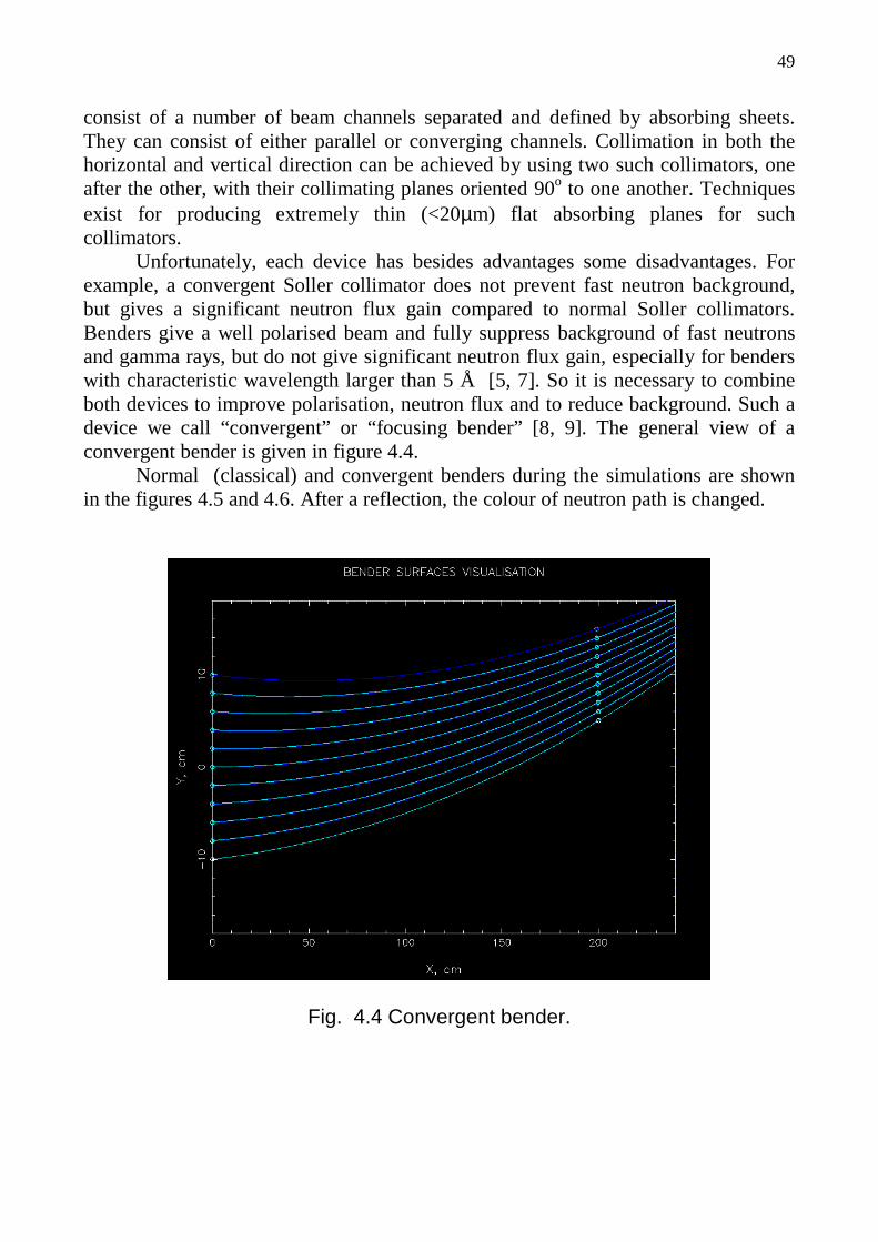
49

consist of a number of beam channels separated and defined by absorbing sheets. They can consist of either parallel or converging channels. Collimation in both the horizontal and vertical direction can be achieved by using two such collimators, one after the other, with their collimating planes oriented 90o to one another. Techniques exist for producing extremely thin (<20µm) flat absorbing planes for such collimators.

Unfortunately, each device has besides advantages some disadvantages. For example, a convergent Soller collimator does not prevent fast neutron background, but gives a significant neutron flux gain compared to normal Soller collimators. Benders give a well polarised beam and fully suppress background of fast neutrons and gamma rays, but do not give significant neutron flux gain, especially for benders with characteristic wavelength larger than 5 Å [5, 7]. So it is necessary to combine both devices to improve polarisation, neutron flux and to reduce background. Such a device we call “convergent” or “ focusing bender” [8, 9]. The general view of a convergent bender is given in figure 4.4.

Normal (classical) and convergent benders during the simulations are shown in the figures 4.5 and 4.6. After a reflection, the colour of neutron path is changed.

Fig. 4.4 Convergent bender.

50

Fig. 4.5 Normal (classical) bender during simulations with neutron flight paths.

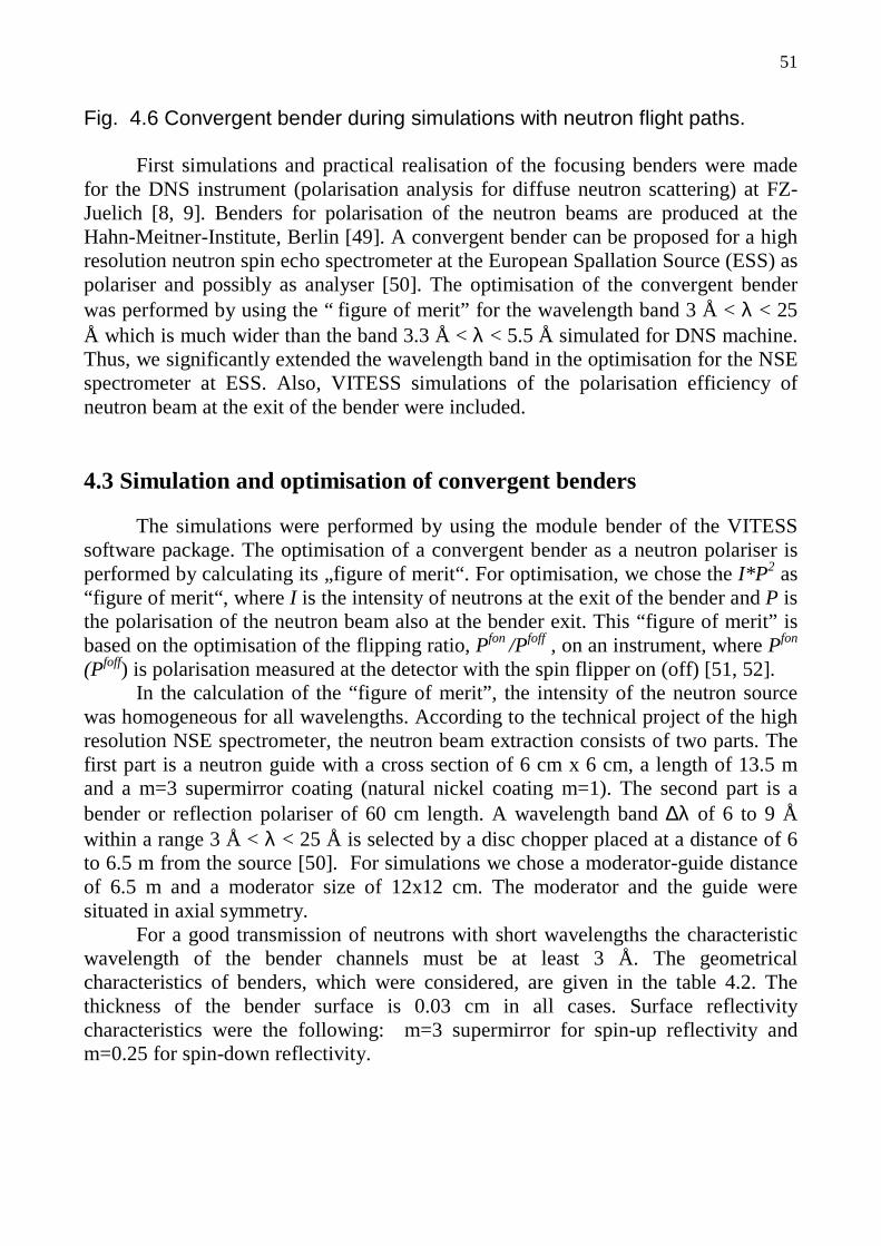
51

Fig. 4.6 Convergent bender during simulations with neutron flight paths.

First simulations and practical realisation of the focusing benders were made for the DNS instrument (polarisation analysis for diffuse neutron scattering) at FZ-Juelich [8, 9]. Benders for polarisation of the neutron beams are produced at the Hahn-Meitner-Institute, Berlin [49]. A convergent bender can be proposed for a high resolution neutron spin echo spectrometer at the European Spallation Source (ESS) as polariser and possibly as analyser [50]. The optimisation of the convergent bender was performed by using the “ figure of merit” for the wavelength band 3 Å < λ < 25 Å which is much wider than the band 3.3 Å < λ < 5.5 Å simulated for DNS machine. Thus, we significantly extended the wavelength band in the optimisation for the NSE spectrometer at ESS. Also, VITESS simulations of the polarisation efficiency of neutron beam at the exit of the bender were included.

4.3 Simulation and optimisation of convergent benders

The simulations were performed by using the module bender of the VITESS software package. The optimisation of a convergent bender as a neutron polariser is performed by calculating its „ figure of merit“ . For optimisation, we chose the I*P2 as “ figure of merit“ , where I is the intensity of neutrons at the exit of the bender and P is the polarisation of the neutron beam also at the bender exit. This “ figure of merit” is based on the optimisation of the flipping ratio, Pfon /Pfoff , on an instrument, where Pfon

(Pfoff) is polarisation measured at the detector with the spin flipper on (off) [51, 52]. In the calculation of the “ figure of merit” , the intensity of the neutron source

was homogeneous for all wavelengths. According to the technical project of the high resolution NSE spectrometer, the neutron beam extraction consists of two parts. The first part is a neutron guide with a cross section of 6 cm x 6 cm, a length of 13.5 m and a m=3 supermirror coating (natural nickel coating m=1). The second part is a bender or reflection polariser of 60 cm length. A wavelength band ∆λ of 6 to 9 Å within a range 3 Å < λ < 25 Å is selected by a disc chopper placed at a distance of 6 to 6.5 m from the source [50]. For simulations we chose a moderator-guide distance of 6.5 m and a moderator size of 12x12 cm. The moderator and the guide were situated in axial symmetry.

For a good transmission of neutrons with short wavelengths the characteristic wavelength of the bender channels must be at least 3 Å. The geometrical characteristics of benders, which were considered, are given in the table 4.2. The thickness of the bender surface is 0.03 cm in all cases. Surface reflectivity characteristics were the following: m=3 supermirror for spin-up reflectivity and m=0.25 for spin-down reflectivity.

52

Number

of bender

Curvature radius for all channels

[cm]

Length of bender [cm]

Channel width at the entrance

[cm]

Channel width at the exit

[cm] 1 500 – 4000 60 0.2 0.1 2 500 – 4000 60 0.2 0.15 3 500 – 4000 60 0.2 0.2 4 500 – 4000 60 0.15 0.15 5 500 – 4000 60 0.15 0.1

Table 4.2 Geometrical data of the simulated benders. The radius of curvature was changed in steps of 500 cm.

The first task was to choose the radius of curvature. The characteristic

wavelength for channels with widths 0.15-0.2 cm and curvature radius 1500 cm have the range 2.77 - 3.2 Å for supermirror m=3. Then the “direct line of sight“ length is within the range 42 - 48 cm. A decreasing radius of curvature worsens the transmission of the bender, but an increasing radius increases the length of “direct line of sight“ . As an optimum we found a bender with a radius of curvature of 1500 cm which completely suppresses the background of fast neutrons and has a good transmission for wavelengths larger than 3 Å.

The second task was to choose the bender with the best “ figure of merit“ from table 4.2 with a radius of curvature of 1500 cm. The wavelength dependence of the “ figure of merit“ is shown in figure 4.7. So we concluded that the optimal bender configuration is the bender No 2 of table 4.2.

As next step in the optimisation we considered two types of coatings. First: spin-up reflectivity of m=3 and spin-down reflectivity of m=0.1; second: spin-up reflectivity of m=3 and spin-down reflectivity m=0.25. The degree of polarisation of the neutron beam at the exit of the guide-bender system as a function of wavelength is shown in figure 4.8. It is necessary to have for most applications a neutron beam with a degree of polarisation of more than 90% for all wavelengths. So we conclude that spin-down reflectivity must be less than m=0.25 for a good degree of polarization for the whole wavelength band. Similar benders may be used as analysers before (usual or positive sensitive) detectors of neutron spin echo spectrometers.

53

2 4 6 8 10 12 14 16 18 20 22 24 260

2

4

6

8

10

12

14

16

18

20

22

24 Bender - 1 Bender - 2 Bender - 3 Bender - 4 Bender - 5

"FIG

UR

E O

F M

ER

IT"

- IP

2 , a.u

.

WAVELENGTH, Å

Fig. 4.7 The wavelength dependence of the „figure of merit“ for benders from

table 4.2 with a radius of curvature of 1500 cm.

2 4 6 8 10 12 14 16 18 20 22 24 260,50

0,55

0,60

0,65

0,70

0,75

0,80

0,85

0,90

0,95

1,00

DE

GR

EE

OF

POL

AR

IZA

TIO

N O

F B

EA

M

WAVELENGTH, Å

Spin-up reflectivity m=3, spin-down reflectivity m=0.1

Spin-up reflectivity m=3, spin-down reflectivity m=0.25

54

Fig. 4.8 The wavelength dependence of the degree of polarisation of the neutron beam at the exit of the bender-polariser.

The important characteristic of a neutron bender is the flux profile at the exit. It

is shown in figure 4.9 for a normal bender (number 3 of table 4.2). This is applied for the whole wavelength band and for different distances between the bender exit and a positive sensitive detector. Figure 4.10 shows the same profile, but for a convergent bender (number 2 of table 4.2). From this figure it is can be found that optimal neutron flux is formed at the distance 60 cm from bender. A second important characteristic is the angular divergence distribution of the neutron beam at the exit of the bender. Unfortunately, a convergent bender increases the divergence in horizontal direction, see figures 4.11 and 4.12. In vertical divergence, there is no such effect. It is understandable, because our convergent bender only compresses in the horizontal plane. So compromises should be found between intensity and divergence during the consideration of convergent guides and benders. It is especially important for small angle neutron scattering (SANS) instruments.

Fig. 4.9 Neutron flux profile for bender 3 of table 4.2.

-15 -10 -5 0 5 10 150,0

5,0x108

1,0x109

1,5x109

2,0x109

2,5x109

NE

UT

RO

N F

LU

X, a

.u.

OFFSET FROM CENTER OF EXIT OF BENDER IN HORIZONTAL DIRECTION, CM (0 - CENTER)

DISTANCE BETWEEN BENDER EXIT AND DETECTOR

Distance - 0 m Distance - 40 cm Distance - 60 cm Distance - 1 m Distance - 2 m Distance - 3 m Distance - 4 m

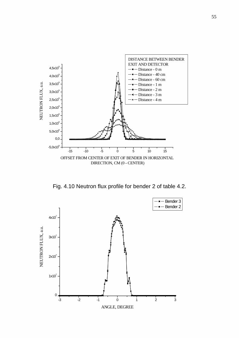
55

Fig. 4.10 Neutron flux profile for bender 2 of table 4.2.

-15 -10 -5 0 5 10 15-5,0x108

0,0

5,0x108

1,0x109

1,5x109

2,0x109

2,5x109

3,0x109

3,5x109

4,0x109

4,5x109

NE

UT

RO

N F

LU

X, a

.u.

OFFSET FROM CENTER OF EXIT OF BENDER IN HORIZONTAL DIRECTION, CM (0 - CENTER)

DISTANCE BETWEEN BENDER EXIT AND DETECTOR

Distance - 0 m Distance - 40 cm Distance - 60 cm Distance - 1 m Distance - 2 m Distance - 3 m Distance - 4 m

-3 -2 -1 0 1 2 30

1x107

2x107

3x107

4x107

NE

UT

RO

N F

LU

X, a

.u.

ANGLE, DEGREE

Bender 3 Bender 2

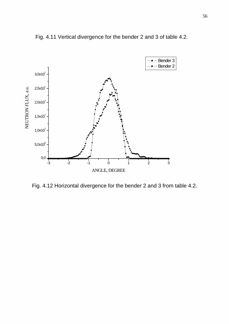
56

Fig. 4.11 Vertical divergence for the bender 2 and 3 of table 4.2.

Fig. 4.12 Horizontal divergence for the bender 2 and 3 from table 4.2.

-3 -2 -1 0 1 2 30,0

5,0x106

1,0x107

1,5x107

2,0x107

2,5x107

3,0x107

NE

UT

RO

N F

LU

X, a

.u.

ANGLE, DEGREE

Bender 3 Bender 2

57

4.4 Summary

Convergent benders will be proposed as neutron polariser and a possible analyser for the high resolution neutron spin echo spectrometer at the European Spallation Source (ESS). We found an optimal configuration of the bender using I*P2 as „ figure of merit“ . To achieve a good polarisation of the beam (>90%) for the whole required wavelength band (3…26 Å), it will be necessary to use a coating with spin-up reflectivity m=3 and spin-down reflectivity less than m=0.1.

58

59

Chapter 5

Simulations of new SANS instrument VSANS with gr id collimation

5.1 Introduction

A new neutron guide hall has been built at the Hahn-Meitner-Institute Berlin for three instruments: a new diffractometer called EXED (Extreme Environment Diffractometer) [11], a new small angle scattering instrument called VSANS [12] and the existing spin-echo instrument SPAN [13]. In this chapter I will consider simulations and analysis of the VSANS beam line and the collimation system of this instrument.

The main goals of this work are:

1. Checking of the correct work of the new ideas behind this instrument;

2. Simulations and analysis of the multi-spectral beam extraction system;

3. Optimisation and analysis of the primary collimation system for the new VSANS instrument;

4. Analytical analysis of the final multiple beam collimation system and comparison with a classical pinhole collimation system;

5. Checking of the performance of the collimation system using Monte Carlo simulations;

6. Finding the robustness of the spectrometer;

Small angle neutron scattering (SANS) [53] is finding applications in an increasing number of subjects: physics, chemistry, biology and applied science. This method investigates structures of a size between and overlapping (for example viruses) those studied by usual crystallography, electron microscopy and provided information not available by other methods. Small angle scattering is achieved by using long wavelength neutrons and relative small scattering angles. Space (or beam

60

hall sizes) limitations and considerations of budget and instrument geometry often limit and significant condition for constructing new small angle scattering machine. To investigate possible design options, Monte Carlo simulations were performed to calculate the performance of a new SANS instrument.

5.2 Simulations of the multi-spectral beam extraction system

The special feature of the new beam line is the multi-spectral beam extraction system [15], which will give the possibility to use neutrons from both moderators: cold and thermal. Prof. F. Mezei proposed realisation of the multi-spectral beam extraction for the ESS is based on using a supermirror plate (m=3) deposited on a thin, transparent silicon substrate which acts as a wavelength dependent switch between the cold and thermal neutrons. After the extraction system, a beam splitter is installed, which divides the guides into two paths: one to the new diffractometer EXED and one to SPAN, VSANS and the reflectometer V6. The principal scheme of the beam hall is given in figure 5.1. The size of the thermal moderator is 60x60 cm2 and the center of the moderator is situated at the origin of the axis OY. The diameter of the cold moderator is 15 cm and center is shitted 11 cm relative to the origin (See figure 5.1, axis Y). Wavelength band for simulations was chosen between 1…20 Å.

61

Fig. 5.1 The principal scheme of the new beam lines. Data received from Prof. F. Mezei [54].

The acceptance of neutrons from both moderators is given in figure 5.2. Acceptance means that only neutrons are counted, which can pass through the extraction system. This applies for wavelength range 1…20 Å. As was said in the previous chapter, neutrons which are accepted are transported later on without significant losses. In figures 5.1 and 5.2 it is clearly shown that the sizes of the real moderators are sufficient to avoid neutron losses in the moderators-extraction system. In figure 5.3 the neutron trajectories through the extraction system are visualised. Figure 5.4 shows the count rate at the differents part of the VSANS beam line. One can find that mainly neutrons from cold moderator are passing into the VSANS and SPAN beam lines. This is very suitable for a small angle scattering machine, because such a type of instrument needs mainly cold neutrons for achiving minimum value of wave vector transfer Qmin, see explanations later.

-20 -10 0 10 20100000

1000000

1E7

1E8

1E9

1E10

1E11

Cou

nt ra

te

Offset cm, 0 - central of thermal moderator, 11 cm - center of cold moderator

horizontal divergence vertical divergence

Fig. 5.2 The acceptance of the “multi-spectral” extraction system in both directions. The diameter of the cold moderator is 15 cm and center is shitted 11 cm relative to the origin in the right side. The size of the thermal moderator is 60x60 cm2. The thermal moderator is centered.

62

Fig. 5.3 Visualisation of neutron paths in the beam extraction system. The yellow lines show trajectories after the first reflection, the neutrons fly from the left to the right emerging from the thermal (lower part) and the cold (upper part) moderator.

63

0 2 4 6 8 10 12 14 16 18 20 221000

100000

1E7

1E9

1E11

1E13

1E15

Neu

tron

coun

t rat

e

Wavelength, Å

At the moderator surface Both moderators Cold moderator Warm moderator-------------------------------------------------------

At the exit of the extraction system At the exit of splitter

Fig. 5.4 The count rate at the moderator surface, exit of the extraction system and exit of the splitter for the VSANS beam line. Neutron count rate at the exit of the extraction system proves the efficient performance of the presented beam extraction system: sum of two Maxwell distributions.

5.3 Simulations and optimisation of the pr imary collimation of VSANS beam line

The VSANS beam line consists of seven main paths:

1. Multi-spectral beam extraction system;

2. Splitter with a cross section of 6x10 cm²;

3. Bender of 80 cm length with cross section 4x4 cm²;

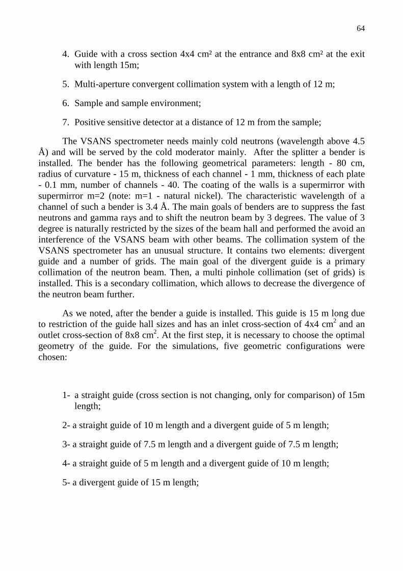
64

4. Guide with a cross section 4x4 cm² at the entrance and 8x8 cm² at the exit with length 15m;

5. Multi-aperture convergent collimation system with a length of 12 m;

6. Sample and sample environment;

7. Positive sensitive detector at a distance of 12 m from the sample;

The VSANS spectrometer needs mainly cold neutrons (wavelength above 4.5 Å) and will be served by the cold moderator mainly. After the splitter a bender is installed. The bender has the following geometrical parameters: length - 80 cm, radius of curvature - 15 m, thickness of each channel - 1 mm, thickness of each plate - 0.1 mm, number of channels - 40. The coating of the walls is a supermirror with supermirror m=2 (note: m=1 - natural nickel). The characteristic wavelength of a channel of such a bender is 3.4 Å. The main goals of benders are to suppress the fast neutrons and gamma rays and to shift the neutron beam by 3 degrees. The value of 3 degree is naturally restricted by the sizes of the beam hall and performed the avoid an interference of the VSANS beam with other beams. The collimation system of the VSANS spectrometer has an unusual structure. It contains two elements: divergent guide and a number of grids. The main goal of the divergent guide is a primary collimation of the neutron beam. Then, a multi pinhole collimation (set of grids) is installed. This is a secondary collimation, which allows to decrease the divergence of the neutron beam further.

As we noted, after the bender a guide is installed. This guide is 15 m long due to restriction of the guide hall sizes and has an inlet cross-section of 4x4 cm2 and an outlet cross-section of 8x8 cm2. At the first step, it is necessary to choose the optimal geometry of the guide. For the simulations, five geometric configurations were chosen:

1- a straight guide (cross section is not changing, only for comparison) of 15m length;

2- a straight guide of 10 m length and a divergent guide of 5 m length;

3- a straight guide of 7.5 m length and a divergent guide of 7.5 m length;

4- a straight guide of 5 m length and a divergent guide of 10 m length;

5- a divergent guide of 15 m length;

65

Natural nickel was chosen as the coating for all guides. Supermirror coated neutron guides are not included in the comparison because of a high divergence of the neutron beam at the exit of such guides and significant costs. Convergent guides should not be considered due to increasing divergence at the exit of such guides or benders. Straight guide is not influence on divergence of a neutron beam during transportation. The vertical and horizontal divergences at the exit of the last guide are presented in figures 5.5 and 5.6.

-2 -1 0 1 20,00E+000

1,00E+008

2,00E+008

3,00E+008

4,00E+008

5,00E+008

6,00E+008

7,00E+008

8,00E+008

9,00E+008

1,00E+009

1,10E+009

Neu

tron

coun

t rat

e

Angle, degree

Straight guide l=15m Straight guide l=10m Divergent guide l=5m Straight guide l=7.5m Divergent guide l=7.5m Straight guide l=5m Divergent guide l=10m Divergent guide l=15m

Fig. 5.5. The beam intensity as a function of the horizontal divergence at the exit of the guide for all wavelength band: 1…20 Å.

66

-2 -1 0 1 20,00E+000

1,00E+008

2,00E+008

3,00E+008

4,00E+008

5,00E+008

6,00E+008

7,00E+008

8,00E+008

9,00E+008

1,00E+009

1,10E+009

Neu

tron

coun

t rat

e

Angle, degree

Straight guide l=15m Straight guide l=10m Divergent guide l=5m Straight guide l=7.5m Divergent guide l=7.5m Straight guide l=5m Divergent guide l=10m Divergent guide l=15m

Fig. 5.6. The vertical divergence at the exit of guide for all wavelength band: 1…20 Å.

So, the optimal guide is a divergent guide of 15 m length. A comparison of the divergence at the exit of the bender and at the exit of the guide also shows that the divergent guide performs a good smoothing of oscillations of the count rate. It is shown in the figure 5.7. This is showing effective work of the primary collimation system. It must be noted that maximal divergences at the exit of the divergent guide are approximately ±1 degree for the horizontal plane and ±1.2 degree for the vertical plane due to gravitation influence. These data will be taken into analytical calculations later on.

As next step, the wavelength distribution of the count rate at the exit of the guide of the five systems was explored. In this case, also only the divergent guide gives a gain in intensity. It is presented in figure 5.8.

67

Fig. 5.7. The vertical and horizontal divergences at the exit of the bender (green and red lines respectively) and the divergent guide for all wavelength bands. Blue line – vertical divergence at the exit of the bender, where is the maximal angle 1.2 degree can be found.

Neutron count rate, log. scale

Angle, degree

Wavelength, Å

Count rate

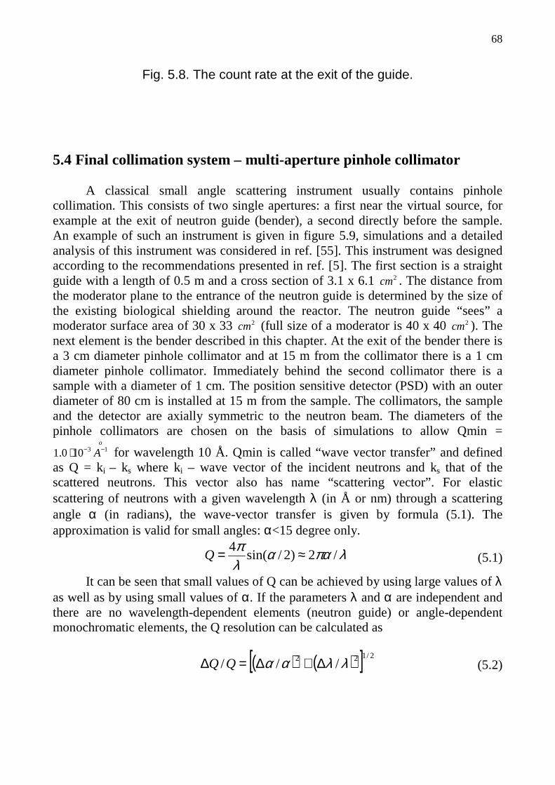
68

Fig. 5.8. The count rate at the exit of the guide.

5.4 Final collimation system – multi-aper ture pinhole collimator

A classical small angle scattering instrument usually contains pinhole

collimation. This consists of two single apertures: a first near the virtual source, for example at the exit of neutron guide (bender), a second directly before the sample. An example of such an instrument is given in figure 5.9, simulations and a detailed analysis of this instrument was considered in ref. [55]. This instrument was designed according to the recommendations presented in ref. [5]. The first section is a straight guide with a length of 0.5 m and a cross section of 3.1 x 6.1 2cm . The distance from the moderator plane to the entrance of the neutron guide is determined by the size of the existing biological shielding around the reactor. The neutron guide “sees” a moderator surface area of 30 x 33 2cm (full size of a moderator is 40 x 40 2cm ). The next element is the bender described in this chapter. At the exit of the bender there is a 3 cm diameter pinhole collimator and at 15 m from the collimator there is a 1 cm diameter pinhole collimator. Immediately behind the second collimator there is a sample with a diameter of 1 cm. The position sensitive detector (PSD) with an outer diameter of 80 cm is installed at 15 m from the sample. The collimators, the sample and the detector are axially symmetric to the neutron beam. The diameters of the pinhole collimators are chosen on the basis of simulations to allow Qmin =

o

A 13100.1 −−⋅ for wavelength 10 Å. Qmin is called “wave vector transfer” and defined as Q = ki – ks where ki – wave vector of the incident neutrons and ks that of the scattered neutrons. This vector also has name “scattering vector” . For elastic scattering of neutrons with a given wavelength λ (in Å or nm) through a scattering angle α (in radians), the wave-vector transfer is given by formula (5.1). The approximation is valid for small angles: α<15 degree only.

λπααλπ

/2)2/sin(4 ≈=Q (5.1)

It can be seen that small values of Q can be achieved by using large values of λ as well as by using small values of α. If the parameters λ and α are independent and there are no wavelength-dependent elements (neutron guide) or angle-dependent monochromatic elements, the Q resolution can be calculated as

( ) ( )[ ] 2/122 /// λλαα ∆+∆=∆ QQ (5.2)

69

For a classical angular pinhole collimation, an optimum choice for the aperture sizes for a given resolution is [56]

)/( 21212 LLLDD += (5.3) where D1 and D2 are the diameters of the first and the second aperture resp., L1

is the distance between the first aperture and the second aperture, L2 is the distance between the sample and the detector.

For a given resolution, magnitude of Q and total length L=L1+L2, the count rate is maximal for [57]:

L1=L2 and D1=2*D2 (5.4) The desirable features for a SANS instrument contain a large wave-vector

range extending to the lowest values of Q, good resolution, low background, high neutron flux at the sample and availability of long wavelength neutrons. All these factors should be considered for constructing a new SANS machine. It should be noted, that in VSANS case the total length of the SANS instrument is restricted.

6.1 cm

3.1 cm

R = 25 m

0.5 m0.6 m

1 collimator

2 collimator

SAMPLE PLANE

MODERATOR SIZE 40 x 40 cm

15 m

DETECTOR PLANE

15 m 1 COLLIMATOR DIAMETER - 3 cm2 COLLIMATOR DIAMETER - 1 cmSAMPLE DIAMETER - 1 cm

5 m

MODERATOR PLANE

Fig. 5.9 Example of a SANS instrument with classical pinhole collimation [55].

The figure 5.10 shows simulations of the presented instrument: direct beam at a

PSD detector. This instrument has two main disadvantages: very significant losses of neutron flux by the collimation, especially for long wavelengths and falling of long

70

wavelength neutrons due to gravity. This falling is increasing a minimum value of wave vector transfer Qmin. It can be found by analysing the figure 5.10. The significant advantage of the given instrument is a low background due to using the bender before the pinhole collimation system. One can found, that this instrument does not satisfy the conditions (5.3) and (5.4) fully, but only partly: distance first collimator-second collimator is equal to the distance sample-detector, i.e. L1=L2, but diameters of collimators have relation 3:1 instead 2:1 as required by the formula (5.4). So count rate will be decreased in comparison with the optimum choice. But if sample diameter will be increased, diameter of direct beam will be increased significantly at a PSD detector.

71

WAVELENGTH 2A WAVELENGTH 6A

WAVELENGTH 8A WAVELENGTH 10A

WAVELENGTH 13A

ο ο

ο

ο ο

Fig. 5.10. The direct neutron beam at the detector. The diameter of the small circle is 8 cm and the diameter of the big circle – is 80 cm. [55]

So, the present instrument is not an optimal choice for VSANS machine. All

presented conditions must be taken into account, especially for a pinhole collimation system.

72

The proposed collimation system for VSANS will have a “ multi converging aper tures” structure [5, 58], see figure 5.11.

Fig. 5.11 Multi pinhole collimation system.

If N single-aperture systems are arranged to produce beams which intersect the sample at slightly different angles, and if these beams all focus to the same point an the detector, the resolution will be practically the same as in a single aperture pinhole collimation system [59, 60]. Multiple aperture grids, all-converging to the same point at the detector (center point), increase the intensity significantly. Intermediate beam grids are required to prevent crossing over from one imaginary channel to another. This effect will be called “cross talk of neutrons” later on. The number of intermediate grids has to be reasonable for preventing the cross talk between channels. The sizes of each hole in the first and the last grid are 0.3 cm and 0.15 cm respectively. The number of holes in each grid is 21x21=441. The distance between holes is 0.085cm for the first grid. The maximal divergences before the first grid are assumed to be 1 degree in horizontal direction and 1.2 degree in vertical direction as received before. The number of intermediate grids, their positions and holes sizes can be evaluated by analytical calculations: recurrent formulas:

Channels, where neutrons Are moving

Detector plane Sample plane

grids

Relative distance

Absolute distance

Center of detector

1243,19 mm

Space between channels

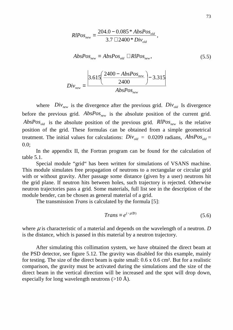
73

,

*24007.3

*085.00.204

old

oldnew Div

AbsPosRlPos

+−=

,newoldnew RlPosAbsPosAbsPos += (5.5)

new

new

new AbsPos

AbsPos

Div

315.32400

2400615.3 −

−

=

where newDiv is the divergence after the previous grid. oldDiv Is divergence

before the previous grid. newAbsPos is the absolute position of the current grid.

oldAbsPos is the absolute position of the previous grid. newRlPos is the relative position of the grid. These formulas can be obtained from a simple geometrical treatment. The initial values for calculations: oldDiv = 0.0209 radians, oldAbsPos = 0.0;

In the appendix II, the Fortran program can be found for the calculation of table 5.1.

Special module “grid“ has been written for simulations of VSANS machine. This module simulates free propagation of neutrons to a rectangular or circular grid with or without gravity. After passage some distance (given by a user) neutrons hit the grid plane. If neutron hits between holes, such trajectory is rejected. Otherwise neutron trajectories pass a grid. Some materials, full list see in the description of the module bender, can be chosen as general material of a grid.

The transmission Trans is calculated by the formula [5]:

)( DeTrans ⋅−= µ (5.6)

where µ is characteristic of a material and depends on the wavelength of a neutron. D is the distance, which is passed in this material by a neutron trajectory.

After simulating this collimation system, we have obtained the direct beam at

the PSD detector, see figure 5.12. The gravity was disabled for this example, mainly for testing. The size of the direct beam is quite small: 0.6 x 0.6 cm². But for a realistic comparison, the gravity must be activated during the simulations and the size of the direct beam in the vertical direction will be increased and the spot will drop down, especially for long wavelength neutrons (>10 Å).

74

Table 5.1. Position of grids and divergences. Negative divergence means changing the velocity direction relative axis of a channel in the grid system.

Number Rel at i ve Di ver gence Di ver gence Absol ut e of gr i d pos i t i on r eal cal cul at ed pos i t i on 1 3. 7876 0. 0209 0. 0777 3. 7876 2 3. 7816 0. 0209 0. 0381 7. 5692 3 3. 7757 0. 0209 0. 0249 11. 3449 4 3. 7697 0. 0183 0. 0183 15. 1146 5 4. 2479 0. 0140 0. 0140 19. 3625 6 5. 4294 0. 0106 0. 0106 24. 7918 7 6. 9315 0. 0080 0. 0080 31. 7233 8 8. 8364 0. 0059 0. 0059 40. 5597 9 11. 2439 0. 0043 0. 0043 51. 8036 10 14. 2736 0. 0030 0. 0030 66. 0772 11 18. 0655 0. 0021 0. 0021 84. 1427 12 22. 7783 0. 0013 0. 0013 106. 9210 13 28. 5838 0. 0007 0. 0007 135. 5048 14 35. 6550 0. 0002 0. 0002 171. 1598 15 44. 1448 - 0. 0001 - 0. 0001 215. 3045 16 54. 1539 - 0. 0004 - 0. 0004 269. 4584 17 65. 6853 - 0. 0006 - 0. 0006 335. 1437 18 78. 5879 - 0. 0008 - 0. 0008 413. 7316 19 92. 4980 - 0. 0009 - 0. 0009 506. 2296 20 106. 7954 - 0. 0010 - 0. 0010 613. 0250 21 120. 5974 - 0. 0011 - 0. 0011 733. 6224 22 132. 8188 - 0. 0012 - 0. 0012 866. 4411 23 142. 3085 - 0. 0012 - 0. 0012 1008. 7496 24 148. 0508 - 0. 0012 - 0. 0012 1156. 8004

75

Fig. 5.12 Direct beam at a PSD detector without gravity for multi pinhole collimation system.

As we can see, the size of the direct beam is much smaller compared with the

pinhole collimation system of the SANS instrument, presented above. This proves the advantage of a multi pinhole collimation system. The other advantage of a multi pinhole collimation is the significant gain in neutron flux for the same size of the direct beam at a PSD detector; in our case it is 0.6x0.6 cm² without the effect of gravity. This can be shown by a comparison of two instruments: the first is the described VSANS instrument and the second is a SANS instrument with standard pinhole collimation. The standard pinhole collimation has to have collimators with sizes 0.3x0.3 cm2 and 0.015x0.015 cm2 respectively. It is mean only one central channel has taken into account. The distance between collimators is the same – 12 m. There are two main characteristics that have to be investigated: the neutron flux at the sample and the size of the direct beam at a PSD detector (or the wave vector transfer Qmin). The sizes of a direct beam at a PSD detector are the same for both machines: 0.6x0.6 cm² as well as resolution. But flux on a sample at least in four hundred times smaller for the standard pinhole collimators machine!

So, it can be found, that if the size of direct beam is decreased, then the flux is decreased too. But a compromise must be found for SANS instruments. In our example, the multi-pinhole collimation system is quite good decision for reducing the sizes of direct beam for a significant sample size 4x4 cm².

If gravity is activated for simulations (what is always the case in reality), the direct beam drops. The distribution of count rate at the PSD detector in vertical direction is presented in figure 5.13. This figure shows also the robustness of the VSANS grid system. Robustness means that the instrument works, even if the grids are installed with some deviations from the ideal grid positions. Of course, this will happen in real life, so the question of robustness of the VSANS machine is very important. The black lines represent the count rate distribution for an ideal system, i.e. distances and sizes of grid were taken from the table 5.1. The red line represents the same distribution, but with a random relative changing of the distances between the grids with 5%. As can be seen, the presented grid system is a quite robust installation.

76

Fig. 5.13 Count rate in vertical direction at the PSD detector.

The robustness of the spectrometer for count rate, depending on the wavelength has also been explored. Neutrons with different wavelength have a different velocity, so some neutrons can be lost under the influence of gravity. There are two figures 5.14 and 5.15 showing this distribution. Figure 5.14 has a linear (normal) scaling for the vertical axis, whereas figure 5.15 has a logarithmic scaling. It can be found that this system is a quite robust setup for the neutron flux too.

-6 -5 -4 -3 -2 -1 0 1 2100

1000

10000

100000

1000000

INFLUENCE OF GRAVITY

Cou

nt r

ate

at th

e de

tect

or in

ver

tical

dire

ctio

n fo

r fu

ll w

avel

engt

h ra

nge

Shift from center, cm

Ideal system The distance between grids is changed within 5%

77

Fig. 5.14 Count rate at the sample in linear scaling.

Fig. 5.15 Count rate at the sample in logarithmic scaling.

0 2 4 6 8 10 12 14 16 18 20

50000

100000

150000

200000

Cou

nt r

ate

at a

sam

ple

Wavelength, Angs.

Ideal system The distance between grids is changed within 5%

0 2 4 6 8 10 12 14 16 18 20

1000

10000

100000

Cou

nt r

ate

at a

sam

ple

Wavelength, Angs.

Ideal system The distance between grids is

changed within 5%

78

The vertical and horizontal divergences at the sample are strongly connected with the resolution of the VSANS spectrometer. The vertical and horizontal divergences for the whole wavelength band are given in figure 5.16. The effect of gravity is the reason for the non-symmetrical shape of the vertical divergence.

-0.40 -0.35 -0.30 -0.25 -0.20 -0.15 -0.10 -0.05 0.00 0.05 0.10 0.15 0.2010

100

1000

10000

100000

Neu

tron

cou

nt r

ate

Angle, degree

Horizontal divergence Vertical divergence

Fig. 5.16 The intensity as a function of vertical and horizontal divergence at the exit of the grid system for the whole wavelength band for a sample sizes 4x4cm2.

The last and most important step is the evaluation of the wave-vector transfer

Qmin. According to figure 5.13 and equation (5.1), Qmin = 0.0033 … 0.00067 Å-1 for wavelength range λ = 3 … 15 Å respectively (compared with Qmin = 0.001 Å-1 for wavelength 10 Å for the previously proposed SANS instrument). Maximal value 10 Å was chosen, because no cold moderator has been installed for the previously proposed SANS instrument. This is much better in comparison with the previous SANS instrument. Qmax is defined by the outer size of the PSD detector or additionally installed detectors.

79

5.5 Summary

The simulations show that the neutron flux distribution in the exit of the extraction system is very well suited for the given instruments. We found that sizes of moderators match to the simulated effective moderator (acceptance) of the original extraction system. We have checked and optimised the primary collimation for the planned VSANS instrument. The divergent guide performs an optimal smoothing of the beam divergence after the bender. The performance of the final collimations system (system grids) has been confirmed using Monte Carlo simulations. No cross talks between channels have been found. This multiple beam focusing system is a quite robust setup and provides enhanced intensity at the sample of size 4x4 cm² and a quite small Qmin= 0.0033 … 0.00067 Å-1 for a total short length of final collimation system: (12+12m) compared with Qmin = 0.001 Å-1 for the previously proposed SANS instrument. But for some applications, a pinhole collimator can be installed too. Special module grid has been written for simulations of VSANS instrument by the author of this thesis.

80

81

Chapter 6

Neutron Spin Echo method, classical and resonance spin echo: simulations of Neutron Resonance Spin Echo spectrometer ZETA

6.1 Introduction Nearly 60 years ago Halpern and Johnson published their article [61] on

neutron interaction potentials. They showed that changes in energy and momentum of a neutron scattering of a sample contain information about magnetic and nuclear structure and dynamics of the target. Although it was appreciated that explicit use of the neutron spin as a further experimental parameter would provide a powerful additional probe of magnetic system.

The neutron is a spin ½ particle; hence the cross section for scattering from a sample with a preferred axis will in general depend on the relative orientation of the axis and the neutron spin [62]. This dependence can be quite strong such that the cross section is significant only for one incident spin state. If the incoming beam is polarised, measurement of the cross section as a function of the incident beam polarisation gives additional information on a preferred-axis system.

All precession properties can be described in a classical treatment. Neutron precession can most easily be visualised through a classical treatment. The main reason for this is the fact, that the quantum mechanical treatment by introducing Pauli spin matrices into the Schoedinger equation is effectively a classical treatment if one considers the origin of those matrices. An exception to this is the Stern-Gerlach effect must be excluded from classical treatments [63]. In this work we will only discuss cases without strong magnetic field gradients and consequently the neutron precession is treated classically in all simulations.

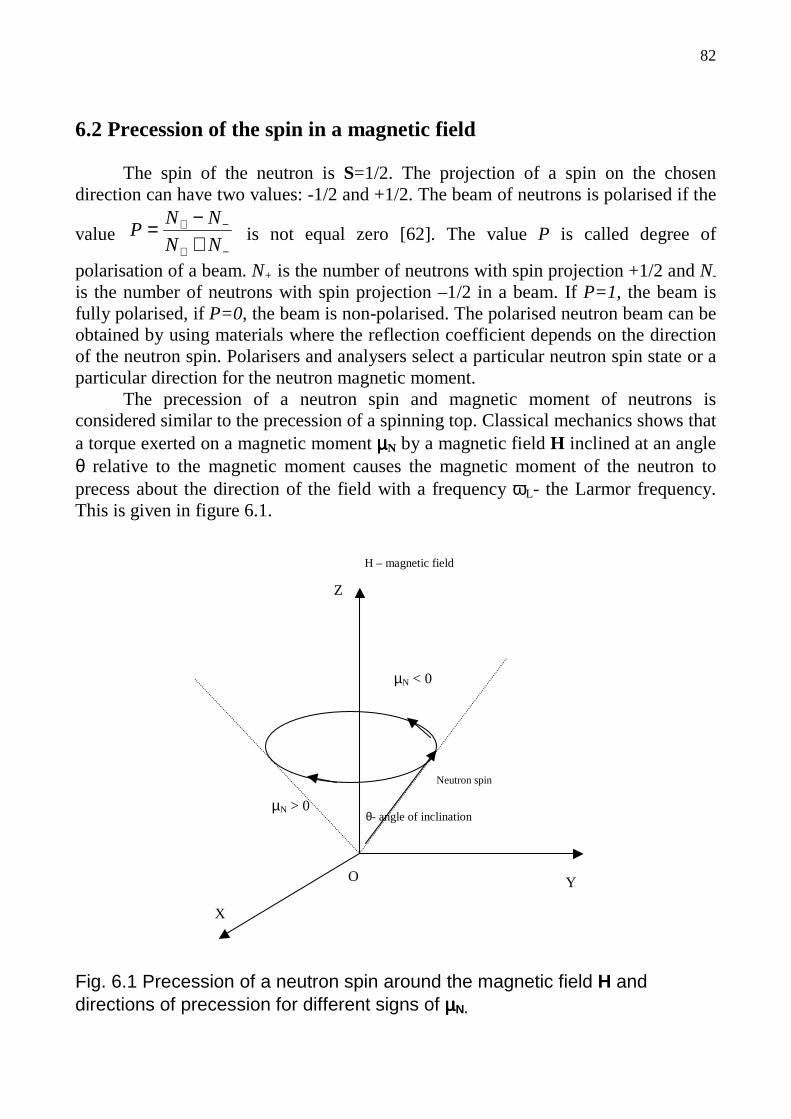
82

6.2 Precession of the spin in a magnetic field

The spin of the neutron is S=1/2. The projection of a spin on the chosen direction can have two values: -1/2 and +1/2. The beam of neutrons is polarised if the

value −+

−+

+−=

NN

NNP is not equal zero [62]. The value P is called degree of

polarisation of a beam. N+ is the number of neutrons with spin projection +1/2 and N- is the number of neutrons with spin projection –1/2 in a beam. If P=1, the beam is fully polarised, if P=0, the beam is non-polarised. The polarised neutron beam can be obtained by using materials where the reflection coefficient depends on the direction of the neutron spin. Polarisers and analysers select a particular neutron spin state or a particular direction for the neutron magnetic moment.

The precession of a neutron spin and magnetic moment of neutrons is considered similar to the precession of a spinning top. Classical mechanics shows that a torque exerted on a magnetic moment µµµµN by a magnetic field H inclined at an angle θ relative to the magnetic moment causes the magnetic moment of the neutron to precess about the direction of the field with a frequency ωL- the Larmor frequency. This is given in figure 6.1.

Fig. 6.1 Precession of a neutron spin around the magnetic field H and directions of precession for different signs of µµµµN.

µN < 0

µN > 0

Y

X

H – magnetic field

O

θ- angle of inclination

Neutron spin

Z

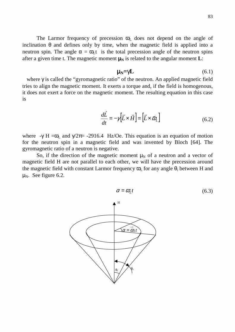
83

The Larmor frequency of precession ωL does not depend on the angle of inclination θ and defines only by time, when the magnetic field is applied into a neutron spin. The angle α = ωLt is the total precession angle of the neutron spins after a given time t. The magnetic moment µµµµN is related to the angular moment L :

µµµµN=γL (6.1) where γ is called the “gyromagnetic ratio” of the neutron. An applied magnetic field

tries to align the magnetic moment. It exerts a torque and, if the field is homogenous, it does not exert a force on the magnetic moment. The resulting equation in this case is

[ ] [ ]LLHLdt

Ld ωγ

×=×−= (6.2)

where -γ H =ωL and γ/2π= -2916.4 Hz/Oe. This equation is an equation of motion for the neutron spin in a magnetic field and was invented by Bloch [64]. The gyromagnetic ratio of a neutron is negative. So, if the direction of the magnetic moment µN of a neutron and a vector of magnetic field H are not parallel to each other, we will have the precession around the magnetic field with constant Larmor frequency ωL for any angle θi between H and µN. See figure 6.2.

tLωα = (6.3)

H

tLωα =

θ1 θ2

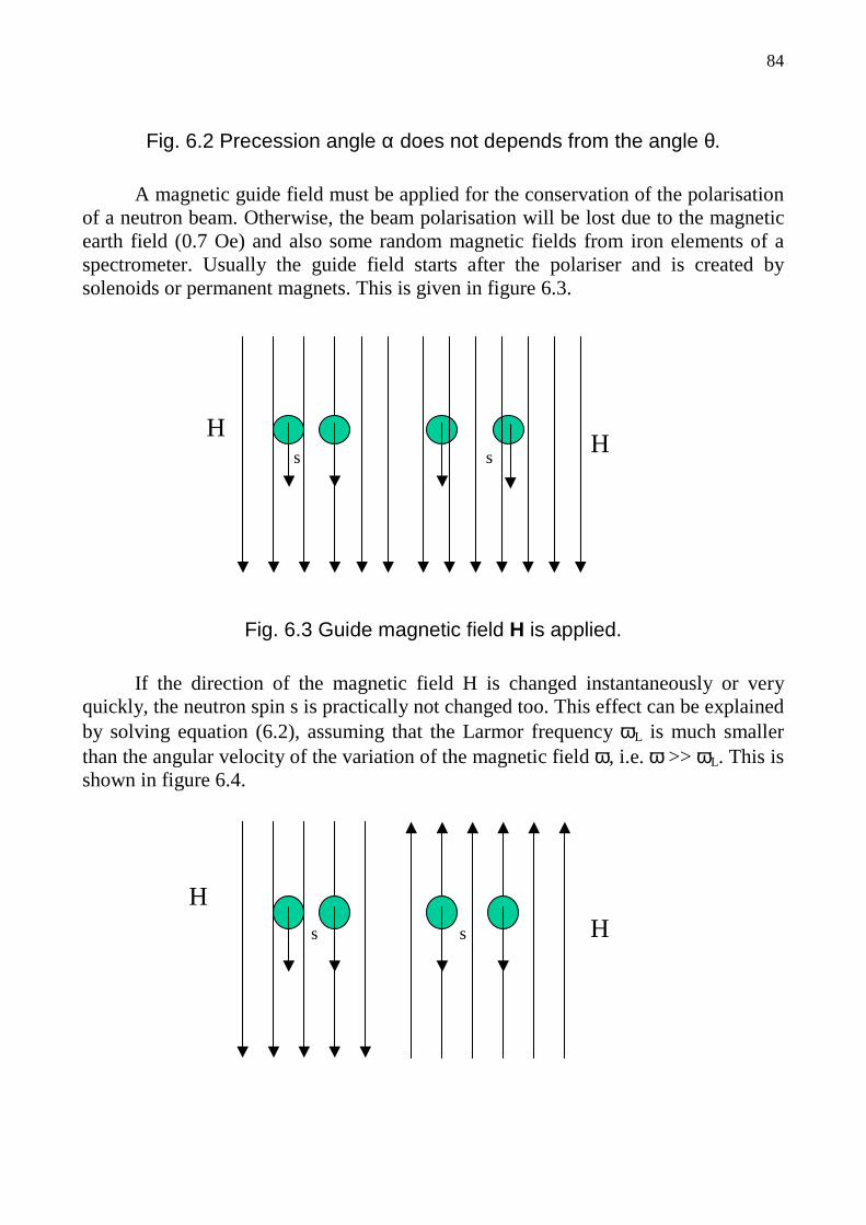
84

Fig. 6.2 Precession angle α does not depends from the angle θ.

A magnetic guide field must be applied for the conservation of the polarisation of a neutron beam. Otherwise, the beam polarisation will be lost due to the magnetic earth field (0.7 Oe) and also some random magnetic fields from iron elements of a spectrometer. Usually the guide field starts after the polariser and is created by solenoids or permanent magnets. This is given in figure 6.3.

Fig. 6.3 Guide magnetic field H is applied.

If the direction of the magnetic field H is changed instantaneously or very quickly, the neutron spin s is practically not changed too. This effect can be explained by solving equation (6.2), assuming that the Larmor frequency ωL is much smaller than the angular velocity of the variation of the magnetic field ω, i.e. ω >> ωL. This is shown in figure 6.4.

HH

s s

HHs s

85

Fig. 6.4 Instantaneous or sudden change of the direction of the magnetic field H. If the direction of the magnetic field changes quite slowly, neutron spins follow the direction of the magnetic field. Slowly changing means, that the Larmor frequency ωL is much large than the angular velocity of the variation of the magnetic field ω, i.e. ω << ωL. This is called adiabatic transition and is shown at the figure 6.5.

Fig. 6.5 The polarisation follows the direction of the magnetic field adiabatically for slowly varying magnetic field H. Let us take an example [42] a flight path of length L = 80 cm and consider that the direction of the magnetic field H and spin s are changed by π/2. The frequency ω is given by:

,8.0

3956

22 λπυπαω

⋅⋅=×==

lt (6.4)

where ν - velocity of the neutron, λ - wavelength of the neutron in Å. For wavelength λ = 5.5 Å, we have ω=1412 s-1. The Larmor frequency ωL is equal to ω for a magnetic field 0.08 Oe. This value of magnetic field is much smaller than even the magnetic earth field, so quite weak magnetic fields can satisfy the condition of adiabaticity for thermal/cold neutrons and can influence the polarisation of neutron beams. This fact proves that the use of magnetic guide fields for polarised neutron beams is obligatory.

L

Direction of flight

H – magnetic field

S -spin

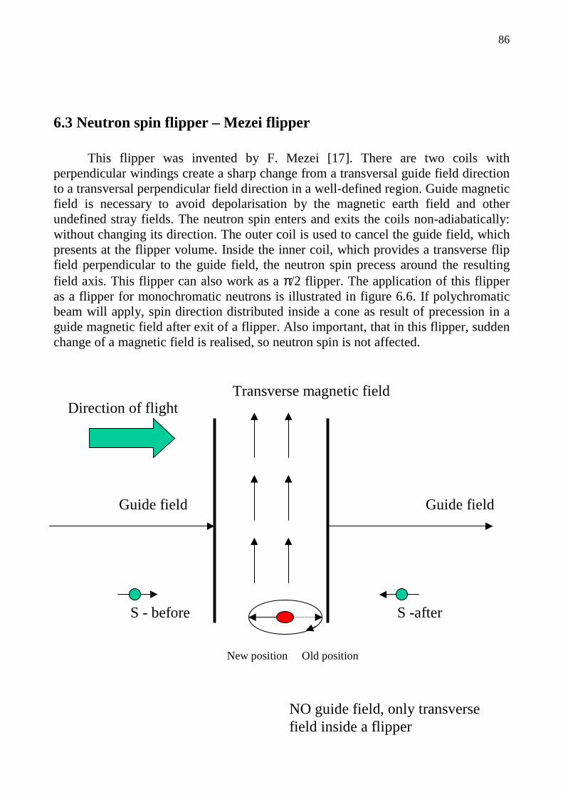
86

6.3 Neutron spin flipper – Mezei flipper

This flipper was invented by F. Mezei [17]. There are two coils with perpendicular windings create a sharp change from a transversal guide field direction to a transversal perpendicular field direction in a well-defined region. Guide magnetic field is necessary to avoid depolarisation by the magnetic earth field and other undefined stray fields. The neutron spin enters and exits the coils non-adiabatically: without changing its direction. The outer coil is used to cancel the guide field, which presents at the flipper volume. Inside the inner coil, which provides a transverse flip field perpendicular to the guide field, the neutron spin precess around the resulting field axis. This flipper can also work as a π/2 flipper. The application of this flipper as a flipper for monochromatic neutrons is illustrated in figure 6.6. If polychromatic beam will apply, spin direction distributed inside a cone as result of precession in a guide magnetic field after exit of a flipper. Also important, that in this flipper, sudden change of a magnetic field is realised, so neutron spin is not affected.

Direction of flight Transverse magnetic field

Guide field Guide field

NO guide field, only transverse field inside a flipper

S - before S -after

New position Old position

87

Fig. 6.6 Application of Mezei coil as a flipper for monochromatic neutrons.

Disadvantages of this sort of flipper include that it requires the guide field compensation coil and procedure of determining the appropriate flip current/wavelength relationship for applying for a time of flight instrument. Also this flipper requires having material in the beam so additional scattering effects could take place.

6.4 Neutron spin echo, general pr incipal The neutron spin echo method is devoted to the investigation of inelastic, quasielastic and even elastic neutron scattering. However this method is principally different from traditional scattering technique. Usually an inelastic neutron experiment is performed by analysis of the neutron energy in the incoming beam and analysis of the energy after scattering by a sample. The smaller the energy change was, the better the neutron speed had to be defined. As the neutron come form a reactor with an approximately Maxwell distribution, an infinitely good energy resolution can be achieved only at the expense of infinitely low count rate of neutron beam at a sample. In 1972 F. Mezei discovered the method of Neutron Spin Echo (NSE) [16]. As we will see in the following this method decouples the energy resolution from intensity losses. In the neutron spin echo technique, the difference in energy of incoming neutrons and scattered neutrons is measured by analysing the Larmor precession of neutron spins: “Larmor clock” . The general layout of a neutron spin echo instrument is presented in figure 6.7. The main parts of the spin echo spectrometer consist of two magnetic field regions with permanent field. The orientation of magnetic field vectors in each region must have different directions. In reality, it is quite difficult to realise such magnetic fields by usual solenoids even with correction coils as in the middle this would create a zero field point where the beam gets easily depolarised [17]. Spin flippers can be used to avoid the orientation of magnetic fields, which is shown in the figure [17, 42]. The π-flipper can reverses the precession plane around.

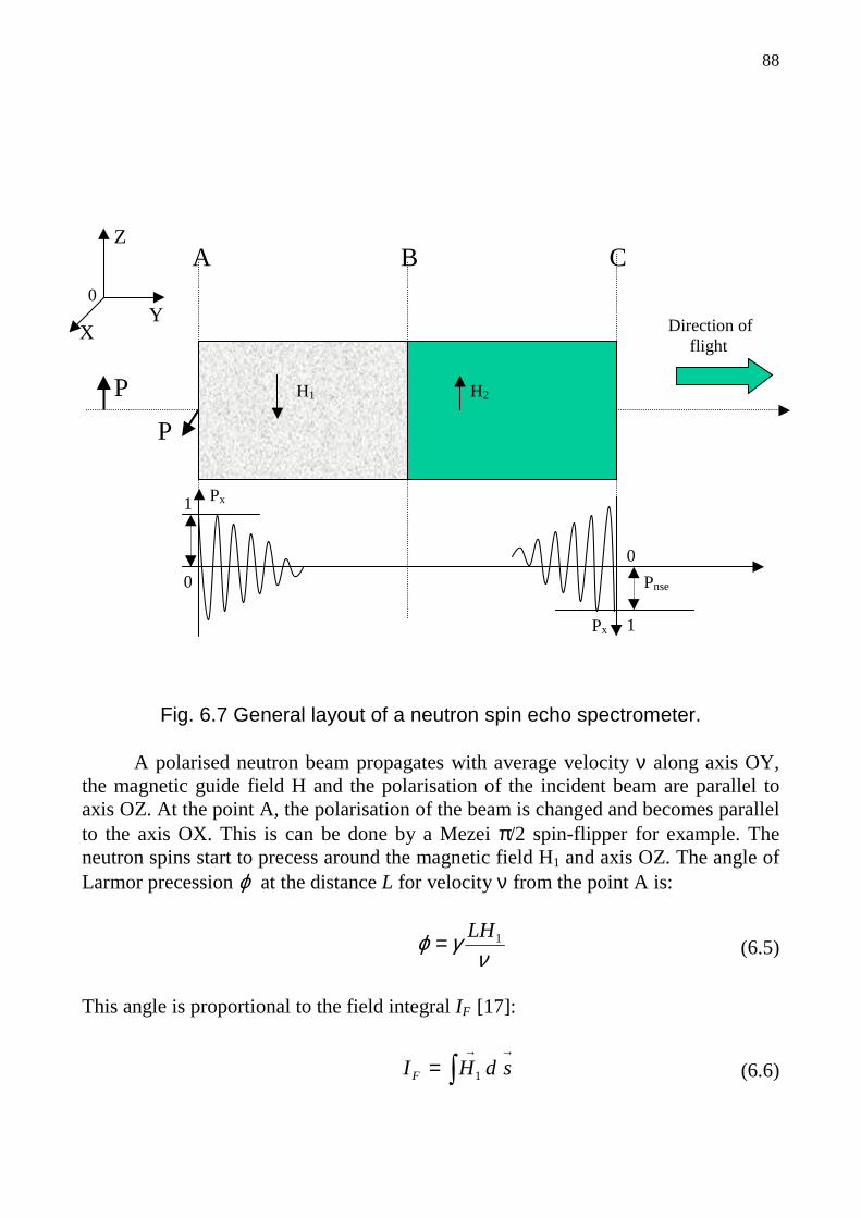
88

Fig. 6.7 General layout of a neutron spin echo spectrometer. A polarised neutron beam propagates with average velocity ν along axis OY, the magnetic guide field H and the polarisation of the incident beam are parallel to axis OZ. At the point A, the polarisation of the beam is changed and becomes parallel to the axis OX. This is can be done by a Mezei π/2 spin-flipper for example. The neutron spins start to precess around the magnetic field H1 and axis OZ. The angle of Larmor precession ϕ at the distance L for velocity ν from the point A is:

νγϕ 1LH= (6.5)

This angle is proportional to the field integral IF [17]:

→→

= sdHI F 1 (6.6)

P

Z

Y X

P

0

Px 1

0

1Px

Pnse

H2 H1

0

A B C

Direction of flight

89

where H1 is a vector of magnetic field, s is a vector of flight path. For an axial trajectory, field integral is H1L and does not depend from the velocity magnitude of a neutron. The beam polarisation after distance l in the magnetic field H1 is given by the cosine of the angle ϕ averaged over the velocity distribution f(ν). The incoming neutron beam is usually monochromatised by a velocity selector [65] and has ±10% deviation around the chosen middle wavelength of a velocity selector.

== νν

γνϕ dlH

fPx1cos)(cos (6.7)

This formula [17] shows the behaviour of the polarisation of a non-monochromatic beam after passing a region with magnetic field. Increasing the distance l, the Larmor precession of spins becomes more and more dephased for different velocities. So value Px becomes more and more close to zero. The analytical approach shows, that we will have oscillations with degraded amplitude for a neutron beam with quite small monochromatisation: ±5…10%, see figure 6.7. The period of the oscillations is defined by the average velocity of the neutrons in the beam. So the velocity or wavelength of the neutrons can be measured by Larmor presession. The first field H1 performs coding operation of an incident beam. The second field H2 is used for the compensation of the dephasing effect due to non-monochromatic incident neutron beam: decoding operation. The direction of precession is changed at the point B to the opposite direction. The neutron magnetic field H2 must be changed instantly at point B. The total precession angle at point C is:

νγϕϕϕ 2211 lHlH

BCAB

−=−= (6.8)

where l1 and l2 are lengths of the magnetic field regions H1 and H2 along the axis OY. So the total precession angle is proportional to the difference between the field integrals in the each field. If 2211 lHlH = , the total precession angle will be ϕ = 0 for ALL wavelengths of the neutrons and Px=1. At the point C, the neutron beam is fully polarised again in the ideal situation. The amplitude of Px can be called spin echo amplitude and designated as PNSE. The sample is installed at the point B. If we will change H2 or l2 and measure Px, the signal, called neutron spin echo signal, will be obtained. If sample changes the velocity and/or direction of neutrons (inelastic and elastic scattering), the spin echo signal will be degraded and/or neutron spin echo signal will be shifted. This is the main idea for analysing neutron scattering by neutron spin echo technique. The neutron time of flight is measured by the angle of

90

precession in the classical neutron spin echo machine. If only the direction of scattered neutrons is changed, it is called “Larmor labelling of angle” . The sensitivity and so the energy resolution of the spin echo method depends from the angle of Larmor precession ϕ (see equation (6.5)) and proportional to the field integral (see equation (6.6)). Magnitudes of a field integral and a wavelength of incident neutrons have to be increased for improving the energy and scattering resolutions of the spin echo method. The general condition for obtaining a spin echo can be described as, final angle of precession at the point C must be same INDEPENDENT of the velocity of neutrons. It is not necessary that total precession angle ϕ is always zero. Analytically it is can be written as [17]:

0=

∂∂

beamνϕ

(6.9)

It is quite difficultly to build a system, which is shown at the figure 6.7. Below after the sample, a neutron π/2 spin flipper can be installed [17, 42]. This flipper must be adjusted for the incident or scattered wavelength. In this case, the change of direction of the magnetic field H2 is not required. The biggest advantage of NSE technique is that it decouples monochromatisation from energy resolution or we do not need very high monochromatisation of an incident neutron beam. The same applies for scattering vector resolution: we do not need very high collimation of an incident neutron beam. But in the last case a NSE spectrometer has to be modified a little bit, see figure 7.10. This NSE system is easily realised and many spin echo machines have built with two big solenoids and additional correction coils (for example Fresnel coils [66]) for improving uniformity of magnetic fields. The technical aspects of building the spin echo machine significantly have been discussed in the literature, for example, a new spin echo machine [67, 68, 69] for the new neutron source SNS in the United States [70]. 6.5 Radio frequency spin flipper The radio frequency or resonance flipper is a flipper with two perpendicular magnetic fields: a radio frequency (RF) field and a permanent field, see figure 6.8. The radio frequency field can be presented as two rotating magnetic fields on two different rotational directions with the same amplitude. Effectively only one rotating field plus a static magnetic field affect the neutron spin [71]. There for only these two fields are considered for the classical precession of neutron spins. The amplitude of the rotating field has to be calculated according to the π-flip condition (perform a half turning) using the formula

dBrotfield γ

πν= (6.10)

91

where ν - velocity of neutron, d – thickness of flipper in the X-direction, γ - gyromagnetic ratio. Due to the periodicity of the rotation, other Brf amplitudes could be accepted:

d

nBrotfield γ

πν= (6.11)

where n=1, 3, 5, …. The second condition, which is called “resonance condition” , is [72]:

γωrotating

permanentH = (6.12)

where ωrotating is angular frequency, Hpermanent is amplitude of static magnetic field. This condition can be obtained by making a transform to a system rotating about the axis OZ. The result shows, that the effect of the rotation of the coordinate system is to

change the resulting field only by the additive the term γωrotating

. Finally the form of

the Bloch equation is obtained. One can found, that for correct operation of such flipper, the direction of rotation and direction of the permanent magnetic field are

related: the vector γωrotating

has to be equal (0, 0, -Bz). If any of the direction were

chosen incorrectly, the flipper is not operating correctly.

RF field

Static field H

ωrf

Two counter rotating fields

O

Y

X

Z

92

Fig. 6.8 Model of a resonance spin flipper. This flipper was described in ref. [4, 74]. The figure 6.10 represents a motion of the magnetic field in a RF flipper. The figure 6.11 represents a motion of the neutron spin in the flipper. Initial polarisation of the neutron beam is Pz = 1. Final polarisation is Pz = -1. Other components of the polarisation are zero. These figures can be obtained either by analytical calculation or by trajectories tracing with the module “rotating field” of VITESS software package. The parameters of the flipper, which has been used: Dimension in the X direction – 3 cm Dimension in the Y direction – 14 cm Dimension in the Z direction – 5.5 cm Number of layers in each direction – 99 (see how module “rotating field” works in chapter 3) Permanent magnetic field – 100 Oe, antiparallel to the axis OZ Amplitude of rotating field – 9.62 Oe Angular frequency – 291640 Hz Resonance wavelength according the equation (6.10) - 2.35 Å These data are satisfied the both resonance condition (6.10) and (6.12).

S. Klimko provided these parameters from neutron resonance spin echo instrument ZETA built by him [4]. The dependence of the polarisation of neutron beam after the flipper on the wavelength (or velocity) shown in figure 6.9. The periodical character of flipping can be explained by an additional revolution with period 2π of rotating in the flipper: π, 3π, 5π, ... So, this flipper can be used for flipping of some discrete set of wavelengths.

This flipper was successfully built, tested and simulated.

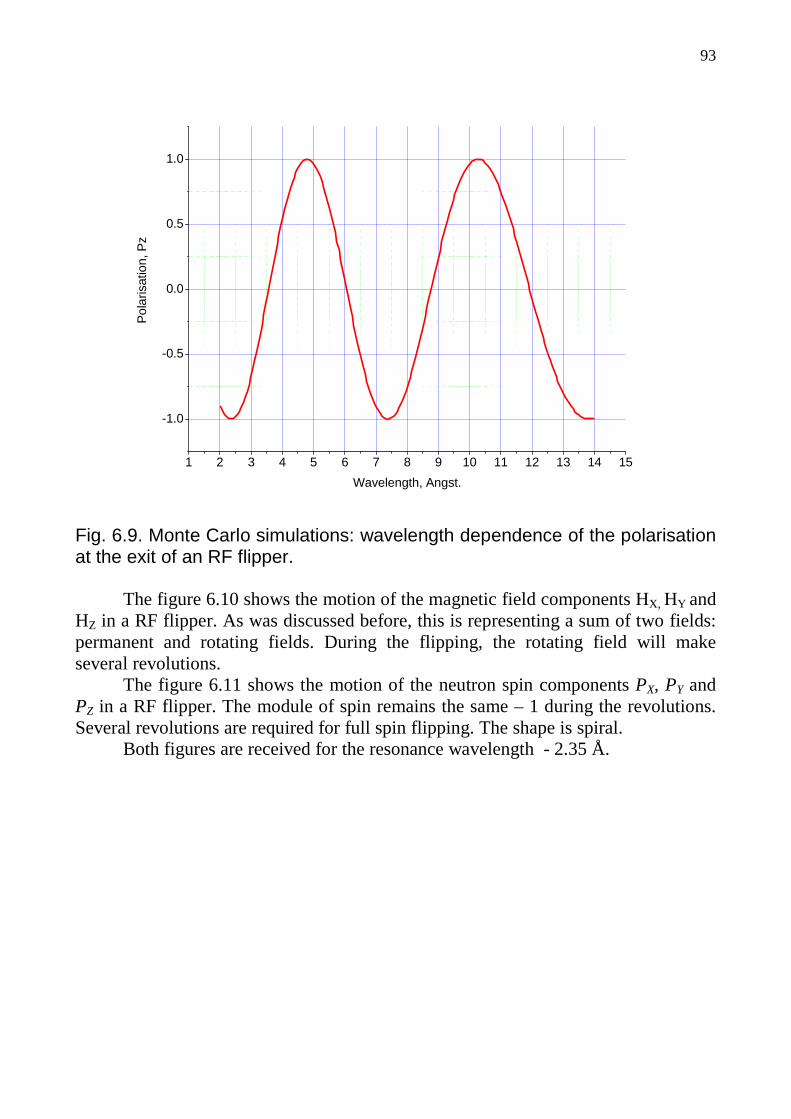
93

1 2 3 4 5 6 7 8 9 10 11 12 13 14 15

-1.0

-0.5

0.0

0.5

1.0P

olar

isat

ion,

Pz

Wavelength, Angst.

Fig. 6.9. Monte Carlo simulations: wavelength dependence of the polarisation

at the exit of an RF flipper.

The figure 6.10 shows the motion of the magnetic field components HX, HY and HZ in a RF flipper. As was discussed before, this is representing a sum of two fields: permanent and rotating fields. During the flipping, the rotating field will make several revolutions.

The figure 6.11 shows the motion of the neutron spin components PX, PY and PZ in a RF flipper. The module of spin remains the same – 1 during the revolutions. Several revolutions are required for full spin flipping. The shape is spiral.

Both figures are received for the resonance wavelength - 2.35 Å.

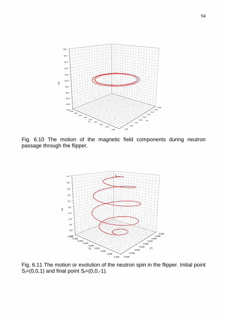
94

-0.08-0.06

-0.04-0.02

0.00

0.02

0.04

0.06

0.08

-101.0

-100.8

-100.6

-100.4

-100.2

-100.0

-99.8

-99.6

-99.4

-99.2

-99.0

-0.08

-0.06

-0.04

-0.02

0.00

0.02

0.040.06

0.08

Hz

HyHx

Fig. 6.10 The motion of the magnetic field components during neutron passage through the flipper.

-0.008-0.006

-0.004-0.002

0.0000.002

0.0040.006

0.008

-1.0

-0.8

-0.6

-0.4

-0.2

0.0

0.2

0.4

0.6

0.8

1.0

-0.008

-0.006

-0.004

-0.0020.000

0.0020.004

0.0060.008

Pz

PyPx

Fig. 6.11 The motion or evolution of the neutron spin in the flipper. Initial point

Si=(0,0,1) and final point Sf=(0,0,-1).

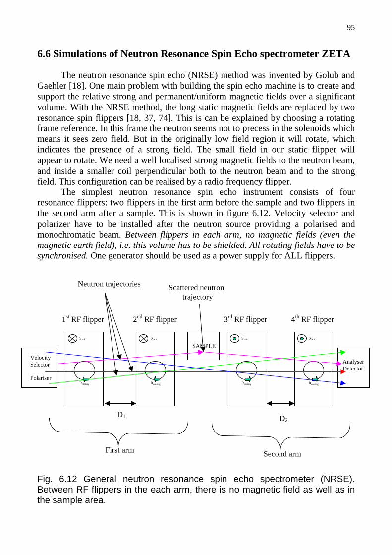
95

6.6 Simulations of Neutron Resonance Spin Echo spectrometer ZETA The neutron resonance spin echo (NRSE) method was invented by Golub and Gaehler [18]. One main problem with building the spin echo machine is to create and support the relative strong and permanent/uniform magnetic fields over a significant volume. With the NRSE method, the long static magnetic fields are replaced by two resonance spin flippers [18, 37, 74]. This is can be explained by choosing a rotating frame reference. In this frame the neutron seems not to precess in the solenoids which means it sees zero field. But in the originally low field region it will rotate, which indicates the presence of a strong field. The small field in our static flipper will appear to rotate. We need a well localised strong magnetic fields to the neutron beam, and inside a smaller coil perpendicular both to the neutron beam and to the strong field. This configuration can be realised by a radio frequency flipper. The simplest neutron resonance spin echo instrument consists of four resonance flippers: two flippers in the first arm before the sample and two flippers in the second arm after a sample. This is shown in figure 6.12. Velocity selector and polarizer have to be installed after the neutron source providing a polarised and monochromatic beam. Between flippers in each arm, no magnetic fields (even the magnetic earth field), i.e. this volume has to be shielded. All rotating fields have to be synchronised. One generator should be used as a power supply for ALL flippers. Fig. 6.12 General neutron resonance spin echo spectrometer (NRSE). Between RF flippers in the each arm, there is no magnetic field as well as in the sample area.

Static

Rotating

Static

Rotating

Static

Rotating

Static

Rotating

SAMPLE

Analyser Detector

Velocity Selector Polariser

First arm Second arm

Neutron trajectories

1st RF flipper 2nd RF flipper 3rd RF flipper 4th RF flipper

D1 D2

Scattered neutron trajectory

96

The first two RF flippers are performing the same task, as a solenoid in a classical spin echo spectrometer. After passage through a solenoid, the precession angle of the neutron spin is given by formula (6.5). For NRSE after first arm, the precession angle is given by:

νω

νγϕ 11 22

DDB rotatingpermanentNRSE == (6.13)

where Bpermanent is static field in the RF flippers, D1 is distance between flippers (not centres of the flippers), ν is velocity of neutron, ωrotating is angular frequency of rotating magnetic field or a RF field. Effective field integral IFE can be calculated as:

12 DI rotatingFE ω= (6.14)

With this method, the time of flight between resonance flippers is measured by the number of revolutions of the rotating magnetic field. All NSE formalism can be applied to NRSE method. The stability of frequency and the homogeneity of the permanent and rotating magnetic fields are essential, but these conditions apply per volume, which is much smaller for NRSE in comparison with the arms in a classical spin echo machine. To satisfy the spin echo focussing condition, the direction of the rotating and permanent magnetic fields have to be changed in the second arm of the NRSE spectrometer. The neutron spin echo focussing does not depends on the initial phase of rotating field at the first (and so other flippers) flipper [74]. If all rotating fields are synchronised, any initial phase will be compensated. The distance D1 or distance D2 can be changed to measure the spin echo signal. This fact can be obtained either analytically or by Monte Carlo simulations. In first case, all incident neutrons have times of flight are zero (or constant value) but different velocities (some distribution) immediately before entering in the first arm of a NRSE or NSE spectrometer. Then polarisation distribution (depending from the velocity or wavelength) should be analysed after the first arm or at a sample: sinusoidal function has to be received. In second case, all incident neutrons have some distribution of times flight as well as velocities. If the same sinusoidal function is obtained again, the spin echo arm operates correctly and spin echo focussing effect will take place [73]. This approach is very useful for checking the correct operating of a new spin echo machine and can be done by VITESS software package easily. The precession angle (and hence field integral or resolution) can be doubled by using a bootstrap technique [37]. The direction of rotating field is changed in the second and third flippers of each arm. The same applies for the direction of

97

permanent field. An analytical approach shows, that the precession angle of a bootstrap NRSE spectrometer is given by:

νω

νγϕ LLB rotatingpermanentNRSEBootstrap 44 ==− (6.15)

So the frequency of the NSE signal from a bootstrap NRSE machine will be doubled.

The bootstrap NRSE technique can be doubled too, so the angle NRSEBootstrap−ϕ is

increased by two times again, however there are practical limits. The first and second arm of the NRSE bootstrap spectrometer is shown at the figure 6.13.

Static

Rotating

Static

Rotating

Static

Rotating

Static

Rotating

First arm

1st RF flipper 2nd RF flipper 3rd RF flipper 4th RF flipper

D1

Static

Rotating

Static

Rotating

Static

Rotating

Static

Rotating

Second arm

1st RF flipper 2nd RF flipper 3rd RF flipper 4th RF flipper

D2

98

Fig. 6.13 First and second arm of an NRSE bootstrap spectrometer The bootstrap NRSE spectrometer ZETA [4], which is considered for Monte Carlo simulations, has 8 flippers, 4 flippers in the each arm. Each flipper has parameters: Dimension in the X direction – 3 cm Dimension in the Y direction – 14 cm Dimension in the Z direction – 5.5 cm Number of layers in each direction – 99 (see how module “rotating field” works in chapter 3) Permanent magnetic field – 246.09 Oe, antiparallel of the axis OZ Amplitude of rotating field – 9.62 Oe Rotation frequency –717700 Hz Resonance wavelength according the equation (6.10) - 2.35 Å No sample – only direct beam

The distance between flippers is 57.5 cm. The incoming wavelength band is 2.35 … 2.352 Å. The divergence of the source is 0.58 degrees in the vertical and horizontal planes. The polarisation of the incoming beam is 54% and 87.4%. The spin echo signal is presented in figure 6.14. Distance between flippers in the second arm changes with step 0.01 cm. Polarised monitors are suggested as ideal. The amplitude of spin echo signal is oscillated due to the beating.

The second example has the same parameters except incoming wavelength band: 2.29 … 2.43 Å. In this case, we will have a decreasing of the amplitude of the spin echo signal due to quite wide velocity or energy range of incident neutrons, see figure 6.15.

The periodicity of the damped oscillation is determined by the average wavelength and the envelope is the Fourier transform of the incoming wavelength distribution.

These dates are fitted quite well into the original measurements presented in ref. [4].

99

57.5 57.6 57.7 57.8 57.9 58.0 58.1 58.2 58.3 58.4 58.5 58.6 58.7 58.8 58.9 59.0

-1.0

-0.8

-0.6

-0.4

-0.2

0.0

0.2

0.4

0.6

0.8

1.0

Pol

aris

atio

n

Distance between flippers in the second arm, D2, cm

Initial polarisation 54% Initial polarisation 87.4%

Fig. 6.14 NSE signal for the incoming wavelength band 2.35 … 2.352 Å.

57.5 57.6 57.7 57.8 57.9 58.0 58.1 58.2 58.3 58.4 58.5 58.6 58.7 58.8 58.9 59.0

-1.0

-0.8

-0.6

-0.4

-0.2

0.0

0.2

0.4

0.6

0.8

1.0

Pol

aris

atio

n

Distance between flippers in the second arm, D2, cm

Initial polarisation 54% Initial polarisation 87.4%

Fig. 6.15 NSE signal for the incoming wavelength band 2.29 … 2.43 Å.

100

6.7 Summary We have described the general principles of precession, neutron spin flippers and spin echo technique and simulated them. Neutron Spin Echo spectrometer measures the time of flight difference of a neutron in the each arm by the “Larmor clock” . The scattering of a neutron in a sample leads into change either wavelength or wave vector. New values (after scattering) of the wavelength and wave vector are connected with the time of flight in the second arm of a NSE spectrometer. There are two main options for realisation of a spin echo machine: classical and resonance spin echo. In the next chapter, we will consider simulation of a new spin echo technique with thin magnetic foils and rotating magnetic field. This new technique is very similar of neutron resonance spin echo machine, but looks simpler for understanding and realisation.

101

Chapter 7

Simulations of Spin Echo spectrometers with rotating magnetic fields 7.1 Introduction

General principles and Monte Carlo simulations of a new spin echo

spectrometer with thin magnetic foils (TMF) and rotating magnetic fields (RMF) are described in this chapter. Dr. A. Ioffe, FZ-Juelich, Germany, suggested the idea of new technique [19]. Author of this thesis made the software development and simulations in collaboration with Dr. A. Ioffe [73]. The new technique is similar to neutron resonance spin echo (NRSE) technique but has some simplifications and can be easily understood. All the NSE and NRSE formalism and applications could be applied for a new spectrometer.

7.2 Thin magnetic film flippers

Consider a thin magnetic foil where the magnetic field vector B rotates with some angular frequency ω in the plane of the foil, see figure 7.1.

Fig. 7.1 The spin flipper with the rotating magnetic field. Rotation of the neutron spin vector is performed by Larmor precession of the neutron spin by the angle π around the magnetic field vector B, as (6.3) equation is required. The angle α is an initial phase of the rotating magnetic field. Initial position of the neutron spin is directed vertically upward (parallel to the axis Z).

z

y

α

2α

s

B

102

When the neutron with initial polarisation along z-axis enters such a foil, the neutron spin vector s precesses around an instant position of the vector B. The precession angle ϕ is defined by the Larmor frequency Lω and the time of the propagation t of the neutron through the foil:

vBdtL γωϕ == (7.1)

where d is the foil thickness; v is the neutron velocity; γ is the gyromagnetic

ratio and B is the amplitude of the rotating magnetic field. If parameters are chosen in such a way that ϕ = π or 3π or 5π… then, when

leaving the foil the neutron spin vector, makes the angle 2α with z-axis. This approach can be called: “Larmor clock or labeling” [73].

It should be noted, that such a flipper can be adjusted and will work only for a single wavelength (flipper for a monochromatic neutron beam). For other wavelengths, the efficiency of the flipper will decrease. Figure 7.2 shows this effect:

15 16 17 18 19 20 21 22 23 24 25

0.50

0.55

0.60

0.65

0.70

0.75

0.80

0.85

0.90

Spi

n co

mpo

nent

s

Wavelength, Angst.

Final spin component Sy Final spin component Sz

Fig. 7.2 The simulation of the thin magnetic field spin flipper with the rotating magnetic field. Amplitude of rotating magnetic field is 3391.19 Oe, frequency is 50 kHz, initial phase α=30 degree. Thickness of the foil is 0.001 cm, the number of layers is 40 along the direction of propagation. The flipper has been adjusted for a wavelength λ≈20Å. The expected spin components for this wavelength: SY=0.866, SZ=0.5 for the instant magnetic field.

103

To obtain the mirror reflection of the neutron spin relative to the magnetic field vector B, this field should not be rotate during the time t =d/ν (d is thickness of the flipper, ν is neutron velocity) of the neutron propagation through the flipper, i.e. ϕ >>ϕB where ϕB is the angle of rotation of a magnetic field and ϕ is a precession angle. So the spin has to see an “ instant magnetic field” theoretically. This condition can also be considered as analytical approach for the adiabatic evolution of the neutron spin in a time-dependent magnetic field. Then the probability for the neutron spin to follow the magnetic field direction is [72]:

2

22

1

12

sin

1)(k

k

kw+

+−=

π

(7.2)

where k = ωL /ωB is the adiabaticity factor, where ωL is Larmor frequency and ωB is frequency of magnetic field rotating. The adiabatic evolution needs k>>1; practically, the adiabatic limit is already approached for k ≥ 4 [72]. It was obtained by analytical solving of the Bloch equation for a rotating magnetic field. Because the Larmor precession angle is equal to π, one can receive:

Bfd

8ν≤ (7.3)

where fB = 2πωB is the frequency of the magnetic field rotation. To realise this requirement for a quite high frequency fB , a spin flipper has to be quite thin.

A rotating magnetic field can be obtained in a foil by two driving

electromagnetic fields that are applied in the orthogonal directions sine and cosine or sine (cosine) shifted in phase by π/2 [73]. This is given in figure 7.3. Special foils (for example produced from metal-glass) are required for amplification of the amplitude of the rotating magnetic field inside a foil [73].

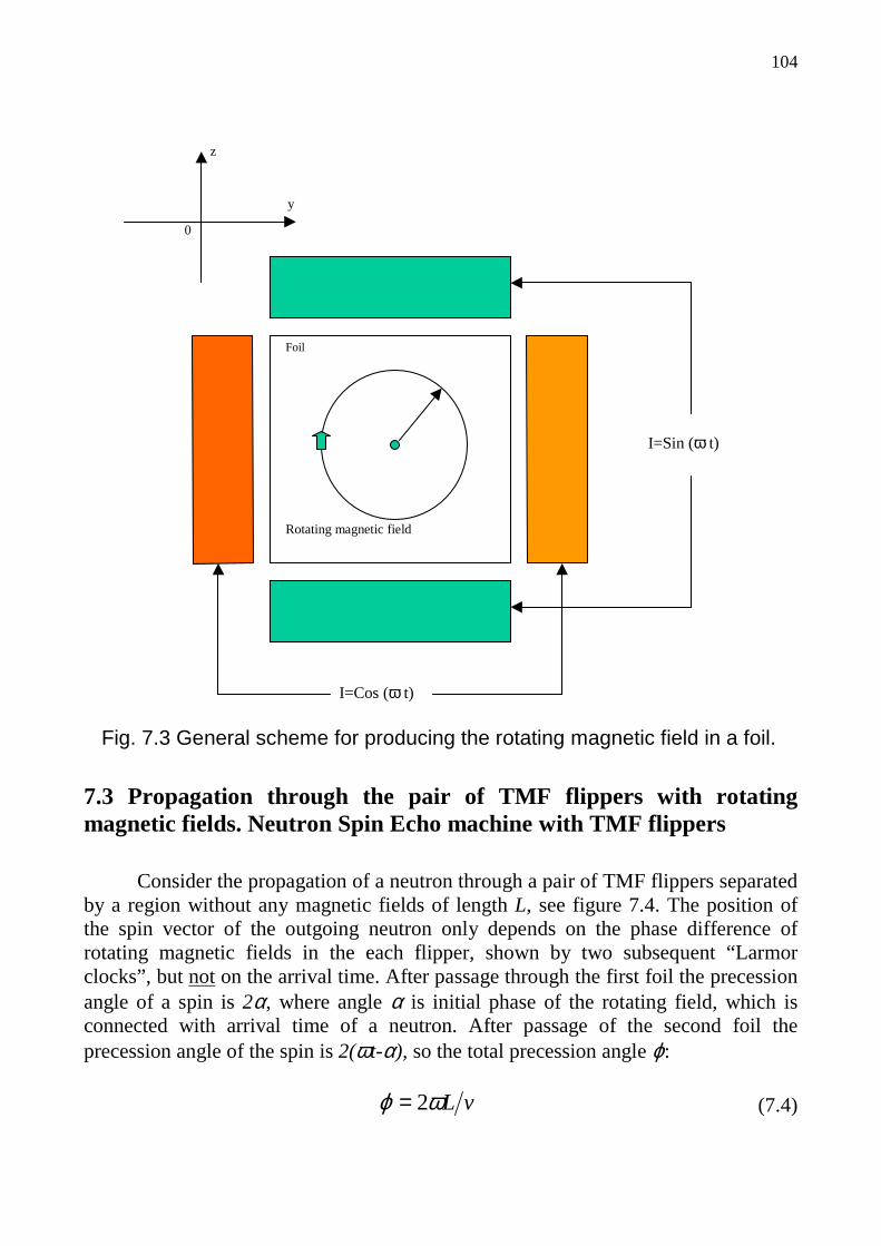
104

Fig. 7.3 General scheme for producing the rotating magnetic field in a foil.

7.3 Propagation through the pair of TMF flippers with rotating magnetic fields. Neutron Spin Echo machine with TMF flippers

Consider the propagation of a neutron through a pair of TMF flippers separated by a region without any magnetic fields of length L, see figure 7.4. The position of the spin vector of the outgoing neutron only depends on the phase difference of rotating magnetic fields in the each flipper, shown by two subsequent “Larmor clocks” , but not on the arrival time. After passage through the first foil the precession angle of a spin is 2α, where angle α is initial phase of the rotating field, which is connected with arrival time of a neutron. After passage of the second foil the precession angle of the spin is 2(ωt-α), so the total precession angle ϕ:

vLωϕ 2= (7.4)

Foil

Rotating magnetic field

I=Sin (ω t)

I=Cos (ω t)

0

z

y

105

where ω - is frequency of a magnetic field rotation; ν – velocity of a neutron; L – distance between foils.

Fig. 7.4 Pair of thin magnetic field flippers. Demonstration of the independence of the total precession angle ϕ (see formula (7.4)) from the arrival time of flight of a neutron at the first flipper foil or the initial phase α of the rotating magnetic field.

This completely coincides with the result obtained in [19, 74] and is the basis of the operation of any spin-echo spectrometer: the spin rotation angle only depends on the time of the neutron passage through an arm of a spin echo spectrometer: between π/2-flippers of the classical neutron spin echo spectrometer (NSE), between radio frequency (RF) flippers of the neutron resonance spin echo spectrometer

out

out

L

z B (0)

ω t

z

x

B (t)

α α

Spin

Magnetic field

ωt

Dashed – old positions

Direction of flight

Z Z

Y Y O O

Direction of rotation of the magnetic field

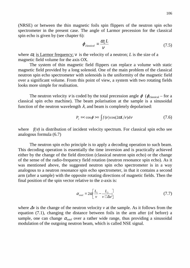
106

(NRSE) or between the thin magnetic foils spin flippers of the neutron spin echo spectrometer in the present case. The angle of Larmor precession for the classical spin echo is given by (see chapter 6):

νωϕ LL

classical = (7.5)

where ωL is Larmor frequency; ν is the velocity of a neutron; L is the size of a magnetic field volume for the axis OX. The system of thin magnetic field flippers can replace a volume with static magnetic field provided by a long solenoid. One of the main problem of the classical neutron spin echo spectrometer with solenoids is the uniformity of the magnetic field over a significant volume. From this point of view, a system with two rotating fields looks more simple for realisation.

The neutron velocity ν is coded by the total precession angle ϕ (ϕclassical – for a classical spin echo machine). The beam polarisation at the sample is a sinusoidal function of the neutron wavelength λ, and beam is completely depolarised:

ννωνϕ dLfPz )2cos()(cos >==< (7.6)

where f(ν) is distribution of incident velocity spectrum. For classical spin echo see analogous formula (6.7)

The neutron spin echo principle is to apply a decoding operation to such beam.

This decoding operation is essentially the time inversion and is practically achieved either by the change of the field direction (classical neutron spin echo) or the change of the sense of the radio-frequency field rotation (neutron resonance spin echo). As it was mentioned above, the suggested neutron spin echo spectrometer is in a way analogous to a neutron resonance spin echo spectrometer, in that it contains a second arm (after a sample) with the opposite rotating directions of magnetic fields. Then the final position of the spin vector relative to the z-axis is:

∆+−=

vv

L

v

Ltotal

212ωα (7.7)

where ∆v is the change of the neutron velocity v at the sample. As it follows from the equation (7.1), changing the distance between foils in the arm after (of before) a sample, one can change αtotal over a rather wide range, thus providing a sinusoidal modulation of the outgoing neutron beam, which is called NSE signal.

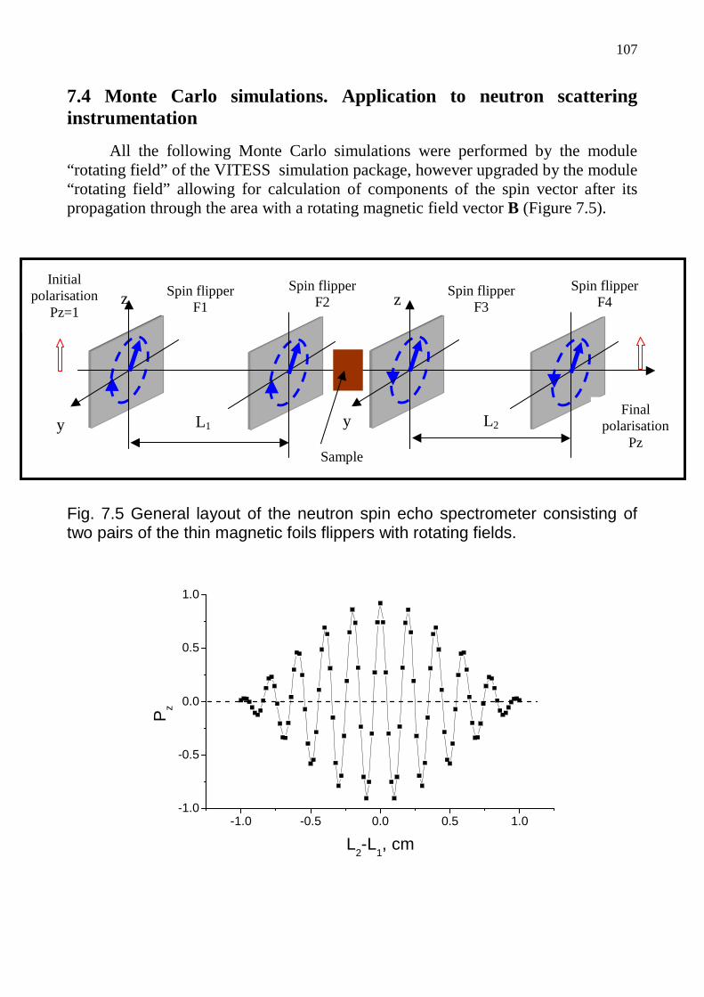
107

7.4 Monte Car lo simulations. Application to neutron scatter ing instrumentation

All the following Monte Carlo simulations were performed by the module “rotating field” of the VITESS simulation package, however upgraded by the module “rotating field” allowing for calculation of components of the spin vector after its propagation through the area with a rotating magnetic field vector B (Figure 7.5).

Fig. 7.5 General layout of the neutron spin echo spectrometer consisting of two pairs of the thin magnetic foils flippers with rotating fields.

-1.0 -0.5 0.0 0.5 1.0-1.0

-0.5

0.0

0.5

1.0

Pz

L2-L

1, cm

z Spin flipper F1

y L1

Spin flipper F2

x

z Spin flipper

F3

y L2

Spin flipper F4

Initial polarisation

Pz=1

Final polarisation

Pz Sample

108

Fig. 7.6 NSE signal obtained for f = 50 kHz and L1 = L2 = 1 m. Neutron wavelength λ0 = 20 Å (∆λ/λ0 = 20%).

The foils’ thickness d = 0.001 cm and the field magnitude B = 3392 Oe are selected to satisfy the spin flip condition ϕ = π only for the central wavelength λ0 = 20 Å. The result of the simulations of the spin-echo signal )( 21 LLfPz −= show the well-known spin-echo signal [17, 66] of a high quality, see figure 7.6.

As it was already mentioned above, the novel NSE technique described here is

essentially a variant of the NRSE technique, however instead of the RF-flippers one uses the thin magnetic fields flippers, where magnetic field vector B rotates with frequency ω in the foil plane. One should note, that the product 2ωL plays the role of the field integral in the NSE technique, thus defining the NSE signal modulation frequency and, indeed, the energy and scattering resolutions of this method. Certainly, the thin magnetic foils to be used are not ideal, for example, it is may have thickness deviations within a few percent. Monte Carlo simulations carried out for the NSE signal (see Figure 7.7) show that random deviations of thickness within 5% from the nominal one results in an insignificant degradation of the amplitude of the NSE signal, thus demonstrating the good robustness of such a NSE spectrometer.

100 .0 100 .5 1 01 .0 101 .5

-1 .0

-0 .5

0 .0

0 .5

1 .0

L2, cm

Pola

riza

tion

Fig. 7.7 Degradation of the NSE signal (open circles) for random deviations within 5% of the foil thickness for all four TMF spin flippers in the NSE

109

spectrometer (Figure 7.5). The solid circles correspond to the ideal NSE signal (Figure 7.6).

This novel NSE technique can be applied in all cases, when the use of Larmor precession devices may result in an improvement either in energy or scattering vector resolution of neutron scattering instruments, particularly for an improvement in the resolution of triple-axis spectrometers [76, 77, 78] or neutron reflectometers [14, 20]. As an example, the sensitivity of the TMF spin flipper NSE setup to inelastic scattering on a sample is illustrated in figure 7.8. Flippers are inclined to underline only sensitivity into energy changing of a NSE spectrometer in case if energy changing on a sample ∆E is depended from the scattering vector Q linearly [17]. As one can see, the energy resolution is increasing up to a few µeV.

0.0 0.1 0.2 0.3 0.4

-1.0

-0.5

0.0

0.5

1.0

Pol

ariz

atio

n

L2 - L

1, cm

∆E = 0 ∆E = 5 µeV ∆E = 10 µeV ∆E = 15 µeV

Fig. 7.8 NSE setup for inelastic scattering. The shift of NSE signal corresponding to the energy exchange ∆E ≈∆ν on the sample. The ν is the neutron velocity, ∆ν is velocity changing of a neutron on the sample. Monte Carlo simulations were carried out for TMF spin flippers (f = 250 kHz)

v

Lt =1 vv

Lt

∆+=2

sample

L L

detector TMF RMF flippers

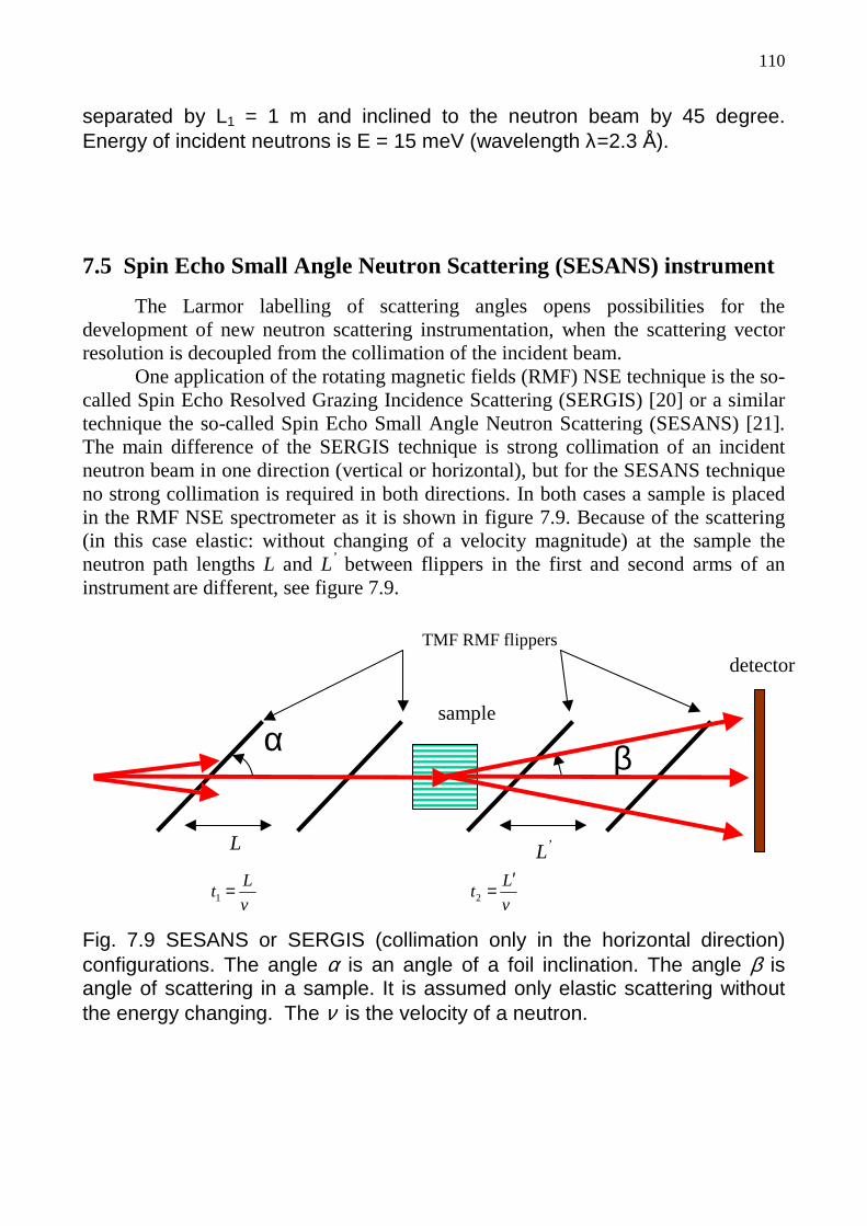
110

separated by L1 = 1 m and inclined to the neutron beam by 45 degree. Energy of incident neutrons is E = 15 meV (wavelength λ=2.3 Å).

7.5 Spin Echo Small Angle Neutron Scatter ing (SESANS) instrument

The Larmor labelling of scattering angles opens possibilities for the development of new neutron scattering instrumentation, when the scattering vector resolution is decoupled from the collimation of the incident beam.

One application of the rotating magnetic fields (RMF) NSE technique is the so-called Spin Echo Resolved Grazing Incidence Scattering (SERGIS) [20] or a similar technique the so-called Spin Echo Small Angle Neutron Scattering (SESANS) [21]. The main difference of the SERGIS technique is strong collimation of an incident neutron beam in one direction (vertical or horizontal), but for the SESANS technique no strong collimation is required in both directions. In both cases a sample is placed in the RMF NSE spectrometer as it is shown in figure 7.9. Because of the scattering (in this case elastic: without changing of a velocity magnitude) at the sample the neutron path lengths L and L’ between flippers in the first and second arms of an instrument are different, see figure 7.9.

Fig. 7.9 SESANS or SERGIS (collimation only in the horizontal direction) configurations. The angle α is an angle of a foil inclination. The angle β is angle of scattering in a sample. It is assumed only elastic scattering without the energy changing. The ν is the velocity of a neutron.

v

Lt =1 v

Lt

′=2

β α

sample

detector

L L’

TMF RMF flippers

111

Fig. 7.10 One (first or second) arm of the SESANS instrument in the case of a classical spin echo setup and a TMF RMF spin echo. The red arrow is a neutron path. Two TMF RMF flippers can be installed instead a magnetic field region, but these flippers and the static magnetic field cannot be used together! The precession angle ϕ can be calculated by the formula (7.1) multiplying by the additional factor (1/sin(α)).

The NSE signal can be recorded by the change of distance L. This sample

works as ideal elastic scatter (velocity and count rate are not changed) for small deviation angles β: 0.01 degree and 0.005 degree. The result of Monte Carlo simulations of corresponding experiment is shown in figures 7.11 and 7.12. NSE signals corresponding to small beam deviations β in the horizontal plane are well resolved in spite of the use of the practically uncollimated, ± 1°, incident neutron beam! We can see a direct proportion between shifting of spin echo signal and deviation angle β changing. This can be explained by following: position of the spin (polarisation) after the propagation through a magnetic field region (see figure 7.10) or after two flippers depends on angles β and α. The total precession angle after passage via an arm can be evaluated analytically [20]:

....)cot1( ++≈== αβλλγωϕ BLh

mBL

v

L nL

.

L

B

Static magnetic field B

OR Two TMF RMF flippers

α

β

112

So, the cotangent of angle α gives possibilities to increase total precession

angle ϕ even for small values of the deviation angle β. The total precession angle ϕ is connected with the effective field integral and hence scattering vector resolution of an instrument.

The phase of NSE signal shifting depends from the angle of inclination of

foils: α (see figures 7.9 and 7.10) and also from the scattering angle. If small value of the angle α is chosen, the phase is increasing and resolution of a spectrometer is improving. Figures 7.11 and 7.12 shows this effect: for the angle α=45° the phase of a spin echo signal is changed smaller than for the angle α=15°. So for improving the resolution, the both sizes of foils have to be increased for SESANS spectrometer or only one size for SERGIS machine. But frequencies of all NSE signals are not changed for the only elastic scattering. The example of the real SERGIS experiment has performed in Hahn-Meitner-Institute, Berlin [79].

100.0 100.2 100.4 100.6 100.8 101.0 101.2 101.4-1.0

-0.8

-0.6

-0.4

-0.2

0.0

0.2

0.4

0.6

0.8

1.0

1.2

1.4

Pol

aris

atio

n P

z

Distance between flippers in the second arm, cm

Spin echo signal - no sample Spin echo signal - deviation angle=-0.01 degree Spin echo signal - deviation angle=0.01 degree Spin echo signal - deviation angle=-0.005 degree Spin echo signal - deviation angle=0.005 degree

Fig. 7.11 Shift of the NSE signals caused by the deviation angles β=±0.01° and β=±0.005° of a practically uncollimated (± 1°) neutron beam in horizontal plane for the RMF flipper`s driving frequency of fB=50kHz, the distance between foils in the first arm is L=1m and the inclination angle of all foils is α=15°. Thickness of all flippers is 0.0025 cm. Incident wavelength band is 3.98 … 4.02 Å.

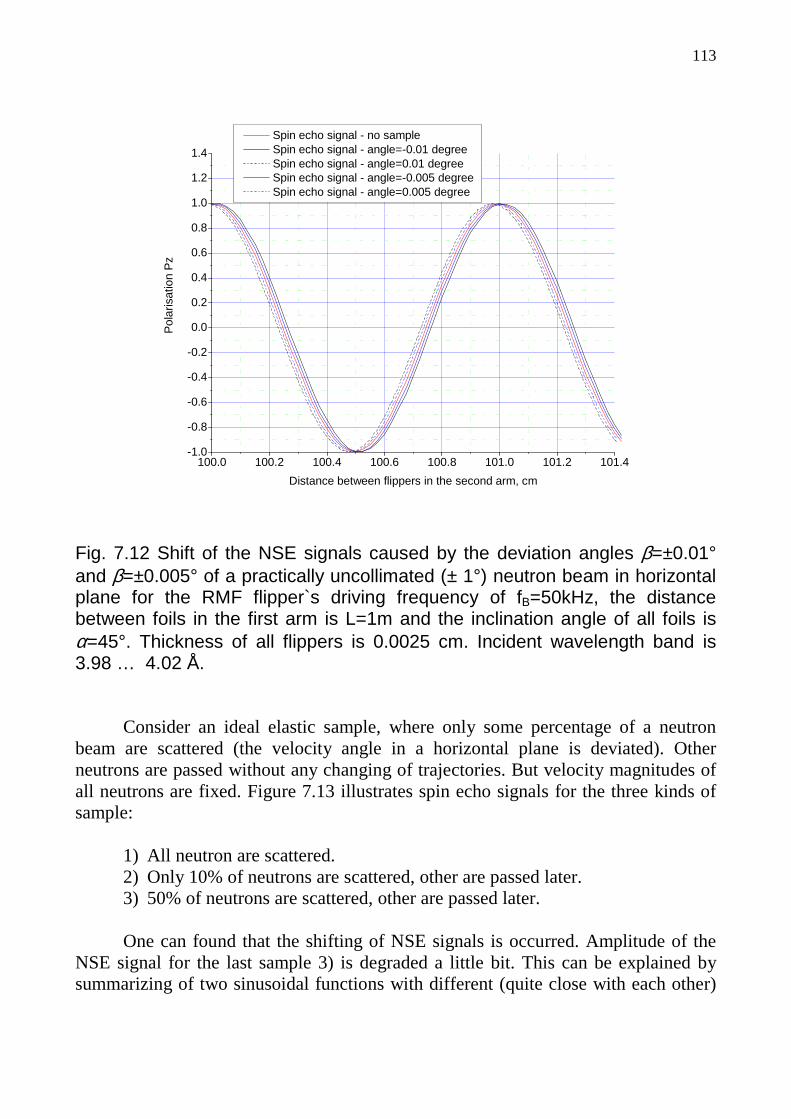
113

100.0 100.2 100.4 100.6 100.8 101.0 101.2 101.4-1.0

-0.8

-0.6

-0.4

-0.2

0.0

0.2

0.4

0.6

0.8

1.0

1.2

1.4P

olar

isat

ion

Pz

Distance between flippers in the second arm, cm

Spin echo signal - no sample Spin echo signal - angle=-0.01 degree Spin echo signal - angle=0.01 degree Spin echo signal - angle=-0.005 degree Spin echo signal - angle=0.005 degree

Fig. 7.12 Shift of the NSE signals caused by the deviation angles β=±0.01° and β=±0.005° of a practically uncollimated (± 1°) neutron beam in horizontal plane for the RMF flipper`s driving frequency of fB=50kHz, the distance between foils in the first arm is L=1m and the inclination angle of all foils is α=45°. Thickness of all flippers is 0.0025 cm. Incident wavelength band is 3.98 … 4.02 Å.

Consider an ideal elastic sample, where only some percentage of a neutron beam are scattered (the velocity angle in a horizontal plane is deviated). Other neutrons are passed without any changing of trajectories. But velocity magnitudes of all neutrons are fixed. Figure 7.13 illustrates spin echo signals for the three kinds of sample:

1) All neutron are scattered. 2) Only 10% of neutrons are scattered, other are passed later. 3) 50% of neutrons are scattered, other are passed later. One can found that the shifting of NSE signals is occurred. Amplitude of the

NSE signal for the last sample 3) is degraded a little bit. This can be explained by summarizing of two sinusoidal functions with different (quite close with each other)

114

phases, but with same frequencies and amplitudes. Of course, after summarizing, the normalization has to be performed.

100.0 100.2 100.4 100.6 100.8 101.0 101.2 101.4

-1.0

-0.8

-0.6

-0.4

-0.2

0.0

0.2

0.4

0.6

0.8

1.0

1.2

1.4

Pol

aris

atio

n P

z

Distance between flippers in the second arm, cm

Spin echo signal - no sample Spin echo signal - only 10% of neutrons are scattered Spin echo signal - only 50% of neutrons are scattered Spin echo signal - All neutrons are scattered

Fig. 7.13 Shift with amplitude degradation of the NSE signals caused by the deviation angles of a practically uncollimated (± 1°) neutron beam in horizontal plane for three kinds of samples, described before. The inclination angle of all foils is α=15°. Thickness of all flippers is 0.0025 cm. The deviation angle is β=0.01°. Incident wavelength band is 3.98 … 4.02 Å.

The similar simulations were performed with a incident neutron beam, which is quite close into the real situation: wavelength band is chosen between 3.6 … 4.4 Å with Maxwell distribution (T=300K) and initial polarisation is 87.5%. The results are given in figure 7.14. Such wavelength band ±10 % around the central wavelength 4 Å can be formed for example by a monochromator. One can found that the spin echo signals are modulated by a dumped function and the amplitude of the all spin echo signals (the maximal value) is practically equal to the initial polarisation: 0.84. But the shifting of the neutron spin echo signals in the horizontal direction still can be recognized. Period of the all spin echo signals is not changed.

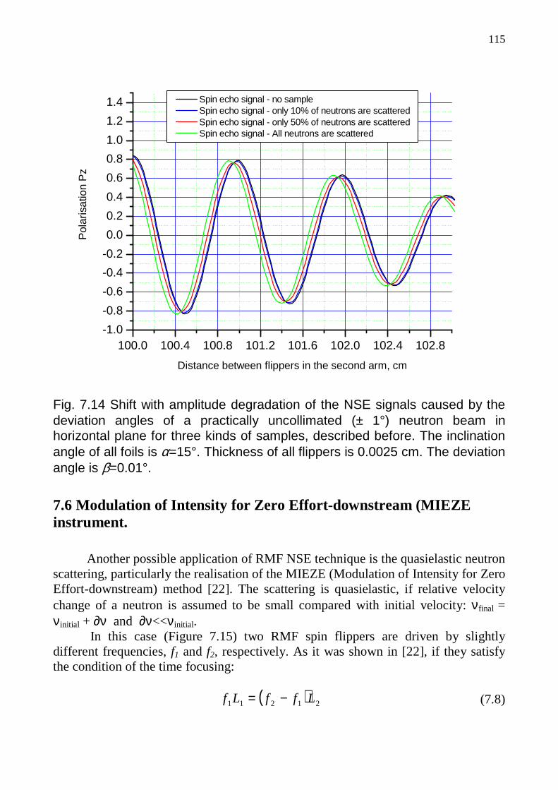
115

100.0 100.4 100.8 101.2 101.6 102.0 102.4 102.8-1.0

-0.8

-0.6

-0.4

-0.2

0.0

0.2

0.4

0.6

0.8

1.0

1.2

1.4

Pol

aris

atio

n P

z

Distance between flippers in the second arm, cm

Spin echo signal - no sample Spin echo signal - only 10% of neutrons are scattered Spin echo signal - only 50% of neutrons are scattered Spin echo signal - All neutrons are scattered

Fig. 7.14 Shift with amplitude degradation of the NSE signals caused by the deviation angles of a practically uncollimated (± 1°) neutron beam in horizontal plane for three kinds of samples, described before. The inclination angle of all foils is α=15°. Thickness of all flippers is 0.0025 cm. The deviation angle is β=0.01°.

7.6 Modulation of Intensity for Zero Effor t-downstream (MIEZE instrument.

Another possible application of RMF NSE technique is the quasielastic neutron scattering, particularly the realisation of the MIEZE (Modulation of Intensity for Zero Effort-downstream) method [22]. The scattering is quasielastic, if relative velocity change of a neutron is assumed to be small compared with initial velocity: νfinal = νinitial + ∂ν and ∂ν<<νinitial.

In this case (Figure 7.15) two RMF spin flippers are driven by slightly different frequencies, f1 and f2, respectively. As it was shown in [22], if they satisfy the condition of the time focusing:

( ) 21211 LffLf −= (7.8)

116

The intensity at the detector does not depend on the wavelength of the incident beam, but beats in time with the frequency ∆f = f1 - f2, so that the instrument may operate with a practically non-monochromatic incident neutron beam. The intensity at the detector is modulated (beating) with frequency ∆f. Any quasielastic scattering at the sample leads to a decrease of amplitude of sinusoidal function at a detector.

Fig. 7.15 General layout of a MIEZE instrument. The red arrow is initial position of neutron spin.

The result of Monte Carlo simulations of the performance of such set up is

shown in figure 7.16. Here RMF spin turners’ driving frequencies are f1 = 50 kHz and f2 = 51 kHz and an incident neutron beam with ∆λ/λ = 20% has been assumed. The focusing effect is observed for L2 /L1 = 50 as it is given by equation (7.8). The time period of oscillations is 1 ms and it corresponds to the difference in frequency ∆f = f2

- f1 = 1 kHz. The measure of the quasielastic scattering is the modulation depth of the intensity oscillations: one may see even for such a modest choice of frequency of the field rotation, the quasielastic scattering with the Lorentz [42] width ∆E of about 1 µeV is detectable. The first red line – no sample.

Polariser

L 2 L 1

f2 f1 TMF flippers

Sample

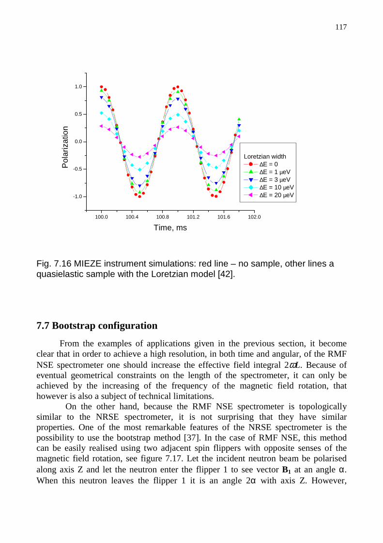
117

Fig. 7.16 MIEZE instrument simulations: red line – no sample, other lines a quasielastic sample with the Loretzian model [42].

7.7 Bootstrap configuration

From the examples of applications given in the previous section, it become clear that in order to achieve a high resolution, in both time and angular, of the RMF NSE spectrometer one should increase the effective field integral 2ωL. Because of eventual geometrical constraints on the length of the spectrometer, it can only be achieved by the increasing of the frequency of the magnetic field rotation, that however is also a subject of technical limitations.

On the other hand, because the RMF NSE spectrometer is topologically similar to the NRSE spectrometer, it is not surprising that they have similar properties. One of the most remarkable features of the NRSE spectrometer is the possibility to use the bootstrap method [37]. In the case of RMF NSE, this method can be easily realised using two adjacent spin flippers with opposite senses of the magnetic field rotation, see figure 7.17. Let the incident neutron beam be polarised along axis Z and let the neutron enter the flipper 1 to see vector B1 at an angle α. When this neutron leaves the flipper 1 it is an angle 2α with axis Z. However,

100.0 100.4 100.8 101.2 101.6 102.0

-1.0

-0.5

0.0

0.5

1.0

Pol

ariz

atio

n

Time, ms

Loretzian width ∆E = 0 ∆E = 1 µeV ∆E = 3 µeV ∆E = 10 µeV ∆E = 20 µeV

118

entering the second flipper it sees the vector B2 at an angle -α with axis Z, so that the angle between the spin vector and B2 is 3α. As the result of the precession it is mirror reflected about B2 and leaves the flipper 2 at an angle -4α with axis Z. Thus, the rotation angle of the spin vector of the outgoing neutron will be doubled with respect to the case of propagation through the single flipper only, which effectively means a doubling of the rotation frequency. Obviously, the third similar flipper will effectively result in tripling the rotation frequency and, generally, N such flippers will provide the effective rotation field frequency of 2Nω. Thus the effective field integral and so the resolution will be N-fold increased, from 2ωL to 2NωL. The arrangement of 10 flippers driven by a current with f = 100 kHz will provide an effective field integral corresponding to f = 1 MHz: it is extremely complicated to achieve such a high frequency of the field by the brutal force approach.

α

2α

s B2

α

4α

z z

n0

Flipper 1 Flipper 2

B1

Fig. 7.17 The bootstrap configuration consist of two closely placed spin flippers with magnetic fields rotating in opposite direction. Open arrows are neutron spin positions. Black arrows are rotating magnetic fields.

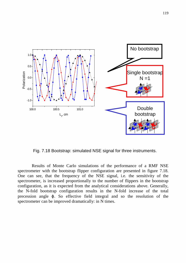
119

Fig. 7.18 Bootstrap: simulated NSE signal for three instruments.

Results of Monte Carlo simulations of the performance of a RMF NSE spectrometer with the bootstrap flipper configuration are presented in figure 7.18. One can see, that the frequency of the NSE signal, i.e. the sensitivity of the spectrometer, is increased proportionally to the number of flippers in the bootstrap configuration, as it is expected from the analytical considerations above. Generally, the N-fold bootstrap configuration results in the N-fold increase of the total precession angle ϕ. So effective field integral and so the resolution of the spectrometer can be improved dramatically: in N times.

100.0 100.5 101.0

-1.0

-0.5

0.0

0.5

1.0

Pol

ariz

atio

n

L2, cm

Double bootstrap

Single bootstrap N =1

No bootstrap

120

7.8 Summary

A new spin echo technique with thin foils and rotating fields has been described. This NSE spectrometer prototype was successfully simulated and looks like quite perspective for future spin echo spectrometers. It can be added to the triple axis machines as spin echo option. We have confirmed robustness of the new spectrometers and presented Monte Carlo simulations of some useful applications: SESANS (SERGIS), MIEZE and Inelastic scattering. Bootstrap option can be used for improving resolution of the spectrometer. This option also was successfully simulated.

121

Chapter 8 Resume

In this thesis, Monte Carlo simulations of neutron scattering spectrometers showed themselves as a flexible and powerful tool for investigation the performance and resolution of the instrument. Additionally simulations were used to confirm new ideas of an instrument.

Monte Carlo simulations were performed by the VITESS software package. As was told by G. Zsigmond (former leader of the VITESS group), the VITESS software package is “some kind” of the neutron instrument. But it is important to understand, that Monte Carlo simulations cannot substitute fully analytical calculations and thinking.

VITESS software package has been developed in Hahn-Meitner-Institute Berlin in cooperation with other institutes such as Paul Scherrer Institute, Switzerland and Institute Laue-Langevin, France. New four modules such as “Bender” , “Rotating field” , “Drabkin resonator” and “Gradient flipper” were written, tested and now ready for using by other users as well as other modules. Simple examples of simulations of the resonator Drabkin and gradient flipper are presented to show the perfect work of these modules.

Module “Bender” is used to simulate and optimise the convergent (or focussing) bender, which is proposed as the neutron polariser or analyser for the high-resolution neutron spin echo spectrometer at the European Spallation Source. Requirement for the geometry and coating material were successfully found as well as other important characteristics of the bender. We have used a coating material with spin-up reflectivity m=3 and spin-down reflectivity less than m=0.1 to obtain a good polarisation (more than 90%) for whole required wavelength band (λ = 3 … 26 Å).

There are different modules used for simulations and optimisaltion of the new small angle scattering spectrometer VSANS, which is building in Hahn-Meitner-Institute, Berlin. The very important part of the VSANS machine are collimators. The simulations and optimisation showed that, the best choice is divergent guide as the primary collimation and the multiple beam focussing system (multiple pinhole system) as the final collimation. Minimum value of the scattering vector evaluated: Qmin = 0.0033 … 0.00067 Å-1 for wavelength range λ = 3 … 15 Å respectively. Final collimation system is quite robust setup.

The second part of the thesis was devoted to Neutron Spin Echo (NSE) technique, which was originally proposed by Prof. F. Mezei in 1972. Neutron Resonance Spin Echo (NRSE) technique, invented by R. Golub and R. Gaehler are

122

also shortly described. The recently build NRSE spectrometer ZETA in institute Laue-Langevin France was simulated successfully by the special written module “Rotating field” and some other additional modules such as source and polarisation monitors.

The new realisation of a spin echo spectrometer proposed by Dr A. Ioffe, FZ-Juelich is successfully simulated by the VITESS module “Rotating field” . This spectrometer consists of four thin magnetic foils with rotating magnetic fields. Monte Carlo simulations showed that this spectrometer is a quite robust setup to the 5% foil variation thickness. Some important applications such as SESANS, MIEZE and inelastic scattering are simulated to confirm the successful operation to as well as bootstrap option of this spectrometer.

VITESS software package will develop in future together with other packages as MCSTAS and RESTRAX and is open for new internal and external users free of charge for simulations and contributions.

123

Chapter 9

Appendix I .

Options for VITESS modules, which are described in the main text, are presented. It can be useful in a case of practical using the VITESS software package. Please note, that “number of domains” here means “number of layers” in the main text.

1. Module “BENDER” .

Parameter Unit Descr iption Command

option

Entrance height [cm]

Size of the bender entrance (in z-direction) -h

Exit height [cm]

Size of the bender exit (in z-direction) -H

Substrate width [cm]

Thickness of the material that separates two neighbouring channels, usually the small part of neutrons passing in the next channel through this material

-s

Length [cm]

Length of the bender -l

Spin up: left, right, top/bottom plane

Reflectivity file for the coating of the bender on the inner side (left), on the outer side (right) and on the top and bottom plane for spin up neutrons

-i, -m, -k

Spin down: left, right, top/bottom plane

Reflectivity file for the coating of the bender on the inner side (left), on the outer side (right) and on the top and bottom plane for spin down neutrons

-I, -M, -K

Surface file File which contains the entrance and exit positions of the channel borders and their radius

-u

Surface waviness [deg]

Waviness of the inner guide surface, i.e. deviations from a perfectly plane surface

-r

Abutment loss length

Neutrons that hit the surface close to one of the ends of the guide (≤ length) are rejected

-a

124

Visualisation Yes: picture of neutron paths will be presented on the given device during the simulations No: no picture is presented

-y

Device Choose the device for the graphic visualisation: 1-display, 2-file, 3-both of them

-o

Polarisation

Yes: splitting into spin up and spin down and using different reflectivity files which depends on the spin state. No: no polarisation is considered, spin-up reflectivity files used for all neutrons

-p

Non-reflected neutrons

Value 0 (No): neutrons, which are not reflected, are absorbed. Value 1 (Yes): neutrons, which were not reflected, are transmitted with the attenuation according the absorption material (see options -z and -w); neutrons, which transmitted through the extreme

surfaces of the bender (left and right), are absorbed.

-g

Test of bender geometry

If activated (value 1), the test of the bender geometry is carried, otherwise is not carried. This is useful for a bender with non-standard geometry. If you have received a warning message, please contact with the author of the module by e-mail: manochine@hmi.de

-t

Number of axis for spin quantisation

This feature uses with polarising neutrons. If spin of neutron is parallel (or antiparallel) of the axis 0X or 0Y or 0Z, this value has to be 0 or 1 or 2 accordingly. The default value is 0 (axis 0X), so the guide magnetic field has to be paralleled to the axis OX

-V

Information file Name of file, which contains some information about the geometry of the bender

-A

Radius of curvature

Radius of curvature of the base circle-axis of the bender (if zero - bender axis is straight line), useful for simulations of Soller collimators

-R

Absorption material in the channel

The absorption coefficient of the material inside of a bender channel. Active, if neutrons can be transmitted between channels of the bender: Option –g1

-c

Transmission file of bender channel

File, which is characterised the transmission of the material inside a bender channel. Active, if options

-C

125

–g is 1 => -g1 and -c is 0 => -c0.

First absorption material

Absorption material in the inner (left) side of the channel; See from the bender entrance - left side. Active, if neutrons are transmitted between channels: Option -g1

-z

Transmission file of left side of channel

File, which is characterised the transmission of material on the left side of channel, see from the entrance. Active, if options -g is 1 => -g1 and –z is 0 => -z0

-T

Second absorption material

Absorption material on the outer (right) side of the channel; See from the bender entrance - right side. Active, if neutrons are transmitted between channels: Option -g1

-w

Transmission file of right side of channel

File, which is characterised the transmission of material in the right side of the channel, see from the entrance. Active, if options -g is 1 => -g1 and –w is 0 => -w0

-O

2. Module “ROTATING FIELD” .

Parameter Unit

Description Command option

Dimensions of field volume X,Y,Z [cm]

Dimension of the common precession volume X,Y,Z

-X, -Y, -V

Position main X,Y,Z [cm]

Centre position of the field volume -k, -l, -m

Offset horiz. [deg]

Horizontal (around vertical axis) rotation angle of the magnetic field volume. This is useful for the simulations of NRSE and/or SESANS instruments

-i

Output X,Y,Z Position of the output frame (in the input -p, -r, -s

126

[cm] frame).

Number of domains in the X direction

Number of domains in the X direction (flight direction)

-C

Number of domains in the Y direction

Number of domains in the Y direction -D

Number of domains in the Z direction

Number of domains in the Z direction -E

Rotating field around given axis

Choose rotating field around of the axis OX or OY or OZ, values 0, 1, 2 respective

-M

Strength of magnetic field [Oe]

Strength (Amplitude) of the rotating magnetic field

-d

Frequency of rotating [Hz]

Rotation frequency of the magnetic field -w

Begin Phase [degree]

Initial phase for rotation -z

File with distribution

Name of a file, which is described the amplitude of the rotating field distribution

-t

Deviation of amplitude [%]

Deviation (or sigma for normal distribution) of the amplitude of the rotating magnetic field

-a

Amplitude distribution

Distribution of the amplitude of the rotating magnetic field Normal_ran Uniform_ran Normal Uniform From_file 0 1 2 3 4

-e

Deviation of frequency [%]

Deviation of the rotation frequency of the magnetic field

-b

Frequency distribution

Distribution of random values: the frequency of the rotating magnetic field Normal Uniform 0 1

-v

TOF from preceding modules

Value 1 – using the time of flight (TOF) from preceding modules for the rotating field phase; Value 0 - No => TOF = 0 for ALL neutrons

-n

Permanent Components X, Y, Z of the permanent -I, -A, -K

127

magnetic field components X, Y and Z [Oe]

magnetic field, which can be added to the components of the rotating magnetic field (projection on a respective axis)

Additional random magnetic field [Oe]

Amplitude of the additional random magnetic field

-q

Output results Output intermediate results of simulations (spin and total magnetic field during the flight) in a file yes no 1 0

-S

Output file: polarisation

Name of the file for output results - spin components

-O

Output file: magnetic field

Name of the file for output results - total magnetic field components

-N

Bootstrap option Activate the bootstrap option -T

Rotating field calculation

Calculating of the amplitude of the rotating field according the given wavelength (Calc. wavelength) and dimension of the common field X (depth) values 0 (no), 1 (yes) to obtain the π-flipping condition.

-x

Calc. wavelength Wavelength for the calculation of conditions for the π-flipping. This option works with the option -x together

-W

3. Module “DRABKIN RESONATOR” .

Parameter Unit

Description Command option

Dimensions of field volume X,Y,Z [cm]

Dimension of the common precession volume X,Y,Z

-X, -Y, -V

Position main X,Y,Z [cm]

Centre position of the field volume. -k, -l, -m

128

Output X,Y,Z [cm]

Position of the output frame (in the input frame).

-p, -r, -s

Number of domains in the X direction

Number of domains in the X direction (flight direction)

-C

Number of domains in the Y direction

Number of domains in the Y direction -D

Number of domains in the Z direction

Number of domains in the Z direction -E

Periodical field parallel to the axis

Periodical field is paralleled to the axis OX, OY or OZ, values 0,1 or 2 respectively

-M

Strength of magnetic field [Oe]

Strength (Amplitude) of the periodical magnetic field

-d

Periodical field changing law

The laws of changing of the amplitude of the periodical magnetic field: uniform (0), sinus (1), gauss (2)

-v

Deviation of amplitude [%]

Deviation of the amplitude of the periodical magnetic field

-a

Amplitude distribution

Distribution of random values: amplitude of the periodical magnetic field: normal (0), uniform (1)

-e

Sigma for gauss distr. [Oe]

Sigma for a gauss distribution of the amplitude of the periodical magnetic field

-x

Permanent or guide magnetic field components X, Y and Z [Oe]

Components X, Y, Z of the permanent (guide) magnetic field, which can be added to the components of the periodical magnetic field (projection in the axis).

-I, -A, -K

Additional random magnetic field [Oe]

Amplitude of the additional random magnetic field

-q

Output results Output intermediate results of simulations: spin and total magnetic field during the flight in the file yes no 1 0

-S

Output file: polarisation

Name of the file for output results - spin components

-O

Output file: magnetic field

Name of the file for output results - total magnetic field components

-N

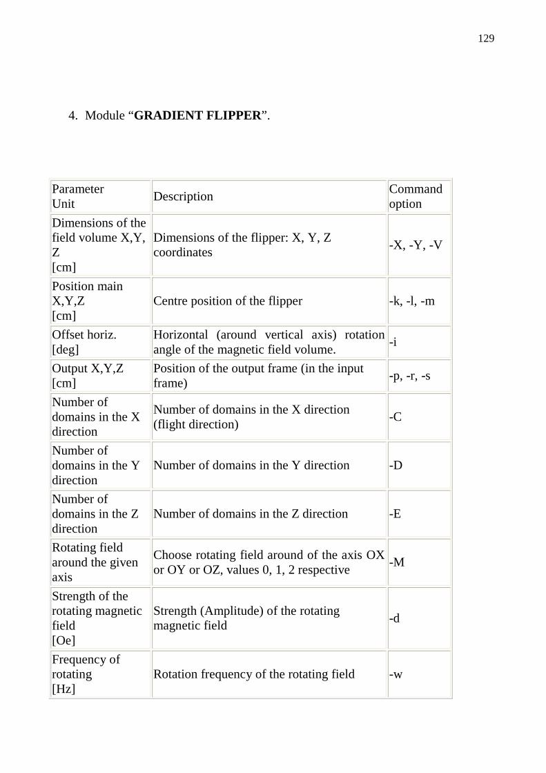
129

4. Module “GRADIENT FLIPPER” .

Parameter Unit

Description Command option

Dimensions of the field volume X,Y, Z [cm]

Dimensions of the flipper: X, Y, Z coordinates

-X, -Y, -V

Position main X,Y,Z [cm]

Centre position of the flipper -k, -l, -m

Offset horiz. [deg]

Horizontal (around vertical axis) rotation angle of the magnetic field volume.

-i

Output X,Y,Z [cm]

Position of the output frame (in the input frame)

-p, -r, -s

Number of domains in the X direction

Number of domains in the X direction (flight direction)

-C

Number of domains in the Y direction

Number of domains in the Y direction -D

Number of domains in the Z direction

Number of domains in the Z direction -E

Rotating field around the given axis

Choose rotating field around of the axis OX or OY or OZ, values 0, 1, 2 respective

-M

Strength of the rotating magnetic field [Oe]

Strength (Amplitude) of the rotating magnetic field

-d

Frequency of rotating [Hz]

Rotation frequency of the rotating field -w

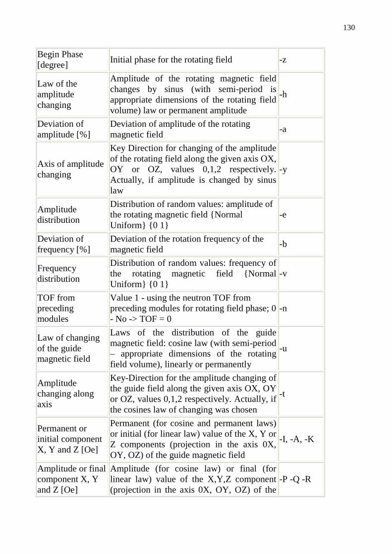
130

Begin Phase [degree]

Initial phase for the rotating field -z

Law of the amplitude changing

Amplitude of the rotating magnetic field changes by sinus (with semi-period is appropriate dimensions of the rotating field volume) law or permanent amplitude

-h

Deviation of amplitude [%]

Deviation of amplitude of the rotating magnetic field

-a

Axis of amplitude changing

Key Direction for changing of the amplitude of the rotating field along the given axis OX, OY or OZ, values 0,1,2 respectively. Actually, if amplitude is changed by sinus law

-y

Amplitude distribution

Distribution of random values: amplitude of the rotating magnetic field Normal Uniform 0 1

-e

Deviation of frequency [%]

Deviation of the rotation frequency of the magnetic field

-b

Frequency distribution

Distribution of random values: frequency of the rotating magnetic field Normal Uniform 0 1

-v

TOF from preceding modules

Value 1 - using the neutron TOF from preceding modules for rotating field phase; 0 - No -> TOF = 0

-n

Law of changing of the guide magnetic field

Laws of the distribution of the guide magnetic field: cosine law (with semi-period – appropriate dimensions of the rotating field volume), linearly or permanently

-u

Amplitude changing along axis

Key-Direction for the amplitude changing of the guide field along the given axis OX, OY or OZ, values 0,1,2 respectively. Actually, if the cosines law of changing was chosen

-t

Permanent or initial component X, Y and Z [Oe]

Permanent (for cosine and permanent laws) or initial (for linear law) value of the X, Y or Z components (projection in the axis 0X, OY, OZ) of the guide magnetic field

-I, -A, -K

Amplitude or final component X, Y and Z [Oe]

Amplitude (for cosine law) or final (for linear law) value of the X,Y,Z component (projection in the axis 0X, OY, OZ) of the

-P -Q -R

131

guide magnetic field

Additional random magnetic field [Oe]

Amplitude of the additional random magnetic field

-q

Output results Output intermediately results of simulations (spin and total magnetic field during flight) in the file yes no 1 0

-S

Output file: polarisation

Name of the file for output results - spin components

-O

Output file: magnetic field

Name of the file for output results - total magnetic field components

-N

132

Appendix I I .

The program calculates the number of intermediate grids, their positions, holes sizes and divergences for new small angle scattering machine VSANS. It is written in FORTRAN language. The results received by the program, are described in chapter 5, see table 5.1 also. PROGRAM calcpass IMPLICIT DOUBLE PRECISION (A-H,O-Z) IMPLICIT INTEGER (I-N)

OPEN(1,FILE='passch.dat') DIVINIT = 0.0209d0 DIVPR = DIVINIT XCURR = 0.0d0 XNEW = 0.0d0 DO I=1,30 XNEW = (204d0-XCURR*0.085d0)/(3.7d0+DIVPR*2400d0) XCURR = XCURR + XNEW DIVPR = (3.615d0*((2400.0d0-XCURR)/(2400.0d0))-3.315d0)/(XCURR) DIVPROLD = DIVPR KEYOV = 0 IF (DIVPR > DIVINIT) THEN DIVPR=0.0209d0 KEYOV = 1 ENDIF WRITE(*,2) I, XNEW, DIVPR, DIVPROLD, XCURR, KEYOV WRITE(1,2) I, XNEW, DIVPR, DIVPROLD, XCURR, KEYOV ENDDO 2 FORMAT(I4,4F15.4, I4) CLOSE(1) END

133

References

[1] D. Wechsler, G. Zsigmond, F. Streffer, F. Mezei, “VITESS: Virtual

Instrumenation Tool for pulsed and Continuous Sources” , Neutron News 11 No. 4,

25-28, 2000.

[2] G. Zsigmond, K. Lieutenant, F. Mezei, Neutron News 13.4, (2002) 11.

[3] H.N. Bordallo et al., Proc. ICANS-XVI, Duesseldorf-Neuss (2003)

[4] S. Klimko PhD thesis ZETA, A zero field spin echo method for very high

resolution study of elementary excitations and first application, TU Berlin 2003.

[5] R. Crawford, J. Carpenter, J. Appl. Cryst. 21, (1988) 589.

[6] T. Krist, C. Lartigue, F. Mezei, Physica B 180-181, (1992) 1005.

[7] A. Schebetov et al., Nucl. Instr. and Meth. A 432, (1999) 214.

[8] W. Hahn, W. Schweika, Physica B 234-236, (1997) 1165.

[9] W. Schweika, P. Böni, Physica B 297, (2001) 155.

[10] http://neutron.neutron-eu.net/n_ess

[11] J. Peters et al., EXED – an instrument in progress, HMI Annual Report (2003)

46.

[12] S. Manoshin et al., MC simulations of new VSANS spectrometer at the Hahn-

Meitner-Institute Berlin, NOBUGS 2004 Conference, PSI, Switzerland, 18-20 Oct.

2004, Poster presentation.

[13] C. Pappas, R. Lischnik, F. Mezei, Physica B 297, (2001) 14.

[14] F. Mezei et al., Physica B 213-214, (1995) 898.

[15] F. Mezei: “The ESS Project Vol II, New Science and Technology for the 21st

Century” , ed. D. Richter (Jülich Germany, 2002) 3; F. Mezei and M. Russina, Patent

application of 23.01.2002, Deutsches patent-u. markenamt, 102 03 591.1

[16] F. Mezei, Z. Physik 255, (1972) 146.

134

[17] In: F. Mezei, Editors, Neutron Spin Echo, Lecture Notes in Physics vol. 128,

Springer, Berlin (1980).

[18] R. Gaeller and R. Golub, Z. Phys. B 65, (1987) 289

[19] A. Ioffe, Physica B 335, (2003) 169.

[20] G. P. Felcher et al., in: Advanced in Neutron Scattering Instrum., SPIE Vol.

4785, (2002) 164.

[21] M. Theo Rekveldt, Nucl. Instrum. Methods B 114, (1996) 366

[22] M. Koeppe et al., Physica B 266, (1999) 75.

[23] G. Zsigmond, K. Lieutenant, “Monte Carlo Simulations of Neutron Scattering

Instruments by VITESS: Virtural Instrumentateion Tool for ESS”, Neutron News 13

No. 4, (2002) 11.

[24] VITESS Website: http://www.hmi.de/projects/ess/vitess

[25]G. Zsigmond, F. Streffer, F. Mezei , “Simulation of the time-of-flight-

backscattering neutron spectrometer IRIS: The Monte Carlo data reduction

technique” , Physica B 276 – 278, (2000) 106.

[26]G. Zsigmond, D. Wechsler, F: Mezei, “Monte Carlo simulation of NSE at reactor

and spallation sources” , Proc. of ICANS-XV, eds. J. Suzuki and S. Itoh, vol. I, 400-

402, Tsukuba, JAERI, (2001)

[27]K. Lieutenant, H. Fritzsche, F. Mezei, “MC simulations of reflectometers at

reactor and spallation sources” , Appl. Phys. A 74 [Suppl.], (2002) 1613.

[28] G. Zsigmond, J. Rodríguez-Carvajal, P.D. Radaelli, K. Lieutenant, F. Mezei,

“MC Simulation of Ultra-high Resolution Powder Diffractometers at a LPSS”, Proc.

ICANS-XVI, eds. G. Mank and H. Conrad, vol. I, 541-547, Düsseldorf, 2003.

[29] K. Lieutenant, T. Gutberlet, A. Wiedenmann, F. Mezei, “Monte Carlo

Simulations of SANS Instruments at ESS”, Nucl. Instr. Meth. Phys. Res. A,

submitted for publication

[30] P.A. Seeger, L.L. Daemon, E. Farhi, W.T. Lee, X.L. Wang, L. Passell, J.

Saroun, G. Zsigmond, “Monte Carlo code comparison for a model instrument” ,

Neutron News 13 No. 4, (2002) 24.

135

[31] G.M. Drabkin, Sov. Phys JETP 16, (1963) 282.

[32] A.N. Bazhenov, V.M. Lobashev, A.N. Pirozhkov and V.N. Slusar, Nucl. Instr.

and Meth. A 332, (1993) 534.

[33] http://www.bellevuelinux.org/pipes.html

[34] M.W. Johnson, “MCGUIDE: A thermal neutron guide simulation program”,

Rutherford Laboratory report RL-80-065, (1980)

[35] http://www.astro.caltech.edu/~tjp/pgplot

[36] http://g2.sourceforge.net

[37] R. Gaehler, R. Golub, J. Phys. France 49, (1988) 1195

[38] S.V. Grigoriev et al., Nucl. Instr. and Meth. A 384, (1997) 451.

[39] H. Maier-Leibnitz, T. Springer, Reactor Sci Technol. 17, (1963) 217.

[40] M.Z. Goldenberger, F. Seitz, Phys Rev 71, (1947) 294. [41] C. J. Carlile, M.W. Johnson, W.G. Williams, Neutron guides on pulsed sources,

Rutherford Laboratory report, RL-79-084, (1979).

[42] A. V. Belushkin, Introduction in neutron scattering methods, Moscow State

University press, (2000), (In Russian).

[43] G. Zsigmond, private communication.

[44] P. Boeni et al., Physica B 267-268, (1999) 320.

[45] C.J. Sutherland, H. Wroe, New methods and Techniques in neutron diffraction,

Report RCN-234, Reactor Centrum Nederland, Petten, (1975) 557.

[46] R.K. Heenan, ICANS-VIII. Proceedings of the Eighth Meeting of the

International Collaboration on Advanced Neutron Sources, Rutherford and Appleton

Laboratories Report, RAL-85-110, (1986) 523.

[47] Manoshin S.A., Belushkin A.V. About calculation of mirror neutron guide by

Monte Carlo method. The advanced version of the program mcguide-new,

Proceeding of 4th conference of young sciences and specialists JINR, Dubna, 2000,

(In Russian).

[48] V.V. Kornilov et al, The characteristics of neutron guides fabricated from FLOAT glass , Preprint JINR, P13-80-496, (1980). [49] T. Krist, Physica B 241-243, (1998) 82.

136

[50] K. Clausen et al., The ESS Project, Instrument and user support, IV (2002) p. 2-

50.

[51] L.D. Cussen et al., Nucl. Instr. and Meth. A 440, (2000) 409.

[52] W.G. Williams, Rutherford Laboratory Report, RL-73-034, (1973).

[53] L. A. Feigin, D.I. Svergun, “Structure analysis by Small Angle X-rays and

Neutron Scattering” , G.W. Taylor (editor), Plenum, (1987).

[54] F. Mezei, private communication.

[55] A.V. Belushkin, S. A. Manoshin, J. Neutr. Res. Vol. 10/2, (2002) 79.

[56] W. Schmatz et al., J. Appl. Cryst. 7, (1974) 96.

[57] D. F. R. Mildner, J.M Carpenter, J. Appl. Cryst. 17, (1984) 249.

[58] J. M. Carpenter, J. Faber Jr., J. Appl. Cryst. 11, (1978) 464.

[59] A. C. Nunes, Nucl. Instrum. Methods 119, (1974) 291.

[60] A. C. Nunes, J. Appl. Cryst. 11, (1978) 460.

[61] O. Halpern, M.H. Johnson, Phys. Rev. 57, (1940) 160.

[62] C. G. Shull et al., Phys. Rev. 84, (1951) 912.

[63] F. Mezei, Lecture Notes of the Introductory Cource to the European Conference

on Neutron Scattering ECNS 99, KFKI-1999-04/E Report, Budapest, (1999) 27.

[64] F. Bloch, W.W. Hansen, M. Packard, Phys. Rev. 69, (1946), 127.

[65] C. D. Clark et al., J. Sci Instrum. 43, (1966) 1.

[66] B. Farago, Lecture Notes of the Introductory Cource to the European Conference

on Neutron Scattering ECNS 99, KFKI-1999-04/E Report, Budapest, (1999) 96.

[67] M. Ohl, M. Monkenbusch, D. Richter, Physica B 335 Iss. 1-4, (2003) 153.

[68] M. Ohl et al., Physica B 350 Iss. 1-3, (2004) 147.

[69] M. Ohl et al., Physica B 356 Iss. 1-4, (2005) 234.

[70] http://www.sns.gov

[71] A. Abragam, Principles of Nuclear Magnetism (Clarendron, Oxford, 1961)

[72] R. Newton, C. Kinel, Phys. Rev. 74, (1948) 1604.

[73] A. Ioffe, private communication.

[74] R. Golub, R. Gähler, Phys. Lett A 123, (1987) 43.

137

[75] R. Gähler, R. Golub, J. Phys. C 3-229, (1984) 45.

[76] T. Keller et al., Physica B 234-236, (1997) 1126.

[77] T. Keller et al., Physica B 241-243, (1997) 101.

[78] S. Klimko et al., Physica B 335 Iss. 1-4, (2003) 188.

[79] J. Major et al., Physica B 336, (2003) 8.

[80] G.S. Bauer, Lecture Notes of the Introductory Cource to the European

Conference on Neutron Scattering ECNS 99, KFKI-1999-04/E Report, Budapest,

(1999) 12.

[81] C. Davisson and L.H. Germer, Phys. Rev. Vol. 30/6, (1927).

[82] http://www.isis.rl.ac.uk

[83] http://www.anl.gov

[84] http://www.kfa-juelich.de/ess/

[85] http://nobelprize.org/physics/laureates/1994/

[86] Meitner, Hahn and Strassman, Zeits. F. Physik 106, (1937) 249

[87] I. K. Vereshagin, Solid State Physics course, publisher “High School” Moscow,

(2001), (in Russian).

The results of this disser tation have been published in:

1) S. Manoshin, G. Zsigmond, K. Lieutenant and F. Mezei, Simulations of a convergent bender as neutron polariser for NSE spectrometers, Physica B: Condensed Matter, Volume 335, Issues 1-4, July 2003, pages 270-273, with poster presentation at the PNCMI 2002 workshop, FZ-Juelich, Germany 2002. 2) S. Manoshin, K. Lieutenant, G. Zsigmond, D. Clemens, F. Mezei, “MC simulations of a new beam line at the Hahn-Meitner-Institute supplied by a multi-spectral beam extraction system”, Proc. ICANS-XVI conference, eds. G. Mank and H. Conrad, vol. I , 513-521, Düsseldorf, 2003 with poster presentation there. 3) Alexander Ioffe and Sergey Manoshin, A neutron spin-echo spectrometer based upon thin magnetic film flippers: the simulation of performance, Physica B: Condensed Matter, Volume 345, Issues 1-4, March 2004, pages 235-238.

138

4) Alexander Ioffe and Sergey Manoshin, Larmor labelling by thin spin flippers with rotating magnetic field: simulations of performance of neutron scattering instruments, Nuclear Instruments and Methods in Physics Research Section A: Accelerators, Spectrometers, Detectors and Associated Equipment, Volume 529, Issues 1-3, August 2004, pages 45-49. 5) A. V. Belushkin and S. A. Manoshin, Simulations of Virtual SANS Spectrometers at IBR-2 Reactor, Journal of Neutron Research, Volume 10 (2) 2002, pages 79-91. Additional poster presentations: 6) A. Ioffe, S. Manoshin, Novel neutron spin echo technique: simulations of performance and applications for neutron scattering, “Polarised Neutrons and Synchrotron X-rays for Magnetism” (international conference), PNSMX 2003, Venice, Italy, 4-6 August 2003. 7) S. Manoshin, G. Zsigmond, K. Lieutenant and F. Mezei, Simulation of polarising convergent benders by VITESS, ESS European Conference, Bonn, Germany, 15 -17 May 2002.

139

Acknowledgements It is my pleasure to thank my colleagues who made this thesis possible: Prof. Dr . Ferenc Mezei, HMI and LANL, for inviting me in Hahn-Meitner-Institute Berlin and for presenting me an opportunity to study and to work in the area of neutron research and Monte Carlo simulations of neutron instruments. I am appreciating his leadership, advices and continuous support. Dr. Geza Zsigmond, PSI (former HMI), the former unofficial leader of the VITESS group. I am especially grateful to him for continuous support and general explanations about the old and present modules of the VITESS software package and for his initial idea to simulate and to optimise a convergent bender for the high-resolution neutron spin echo spectrometer at the ESS. Dr. K laus L ieutenent, ILL (former HMI), for his assistance in the IT concept of the VITESS software package, for helping me with analysis of the obtained data after simulations and for his critical reading and of some chapters and the very valuable advices. Dr. Daniel Clemens, HMI, for valuable discussions during simulations of the new small angle neutron scattering spectrometer VSANS (including beam line) as well as for providing the general concept of the VSANS. Dr. Alexander Ioffe, FZ-Juelich, for valuable discussions about neutron spin echo technique especially with the time-dependant magnetic fields, for his expert supervision during the time of writing, debugging, testing new modules (one of them is “rotating_field” ) and simulating the neutron spin echo instruments with rotating magnetic fields (TMF RMF spectrometer) as well as a gradient flipper. Prof. Giliary Drabkin, HMI and PNPI, for explaining me the general principles of his resonator and for his valuable advices. Dr. Sergey Klimko, PSI and PNPI, for providing me information about the NRSE spectrometer ZETA and RF flippers as well as assistance of simulations of the ZETA spectrometer. Dr. K laus Habicht, HMI, for useful discussions about neutron spin echo technique and his critical reading of some chapters;

140

Dr. Thomas Kr ist, HMI, for providing the data, which describes reflectivity and attenuation of a neutron beam in some materials as well as for testing and using the module “Bender” with his students; Dr. Alexander Belushkin, JINR Dubna, for giving me the first idea to work in the area of Monte Carlo simulations of neutron instruments and his valuable teaching during the my scientific fellow in FLNP JINR Dubna, Russia; HMI – Hahn-Meitnet-Institute, Berlin, Germany; LANL – Los Alamos National Laboratory, USA; FZ-Juelich – Juelich Research Centre, Institute IFF, Germany; PSI – Paul Scherrer Institute, Villingen, Switzeland; ILL – Institute Laue-Langevin, Grenoble, France; PNPI – Petersburg Nuclear Physics Institute, Gatchina, Russia; FLNP JINR, Dubna – Frank Laboratory of Neutron Physics, Joint Institute for Nuclear Research, Dubna, Russia; Finace support was partly provided by the SCANS RTD network and the MCNSI project: The SCANS RTD network is supported by the Access to Research Infrastructures activity, Improving Human Potential programme, of the European Commission under contract HPRI-CT-1999-50013. The MCNSI project is Joint Research Activity under the EU-contract NMI3 (Integrated Infrastructure Initiative for Neutron Scattering and Muon Spectroscopy). Contract Number: RII3-CT-2003-505925

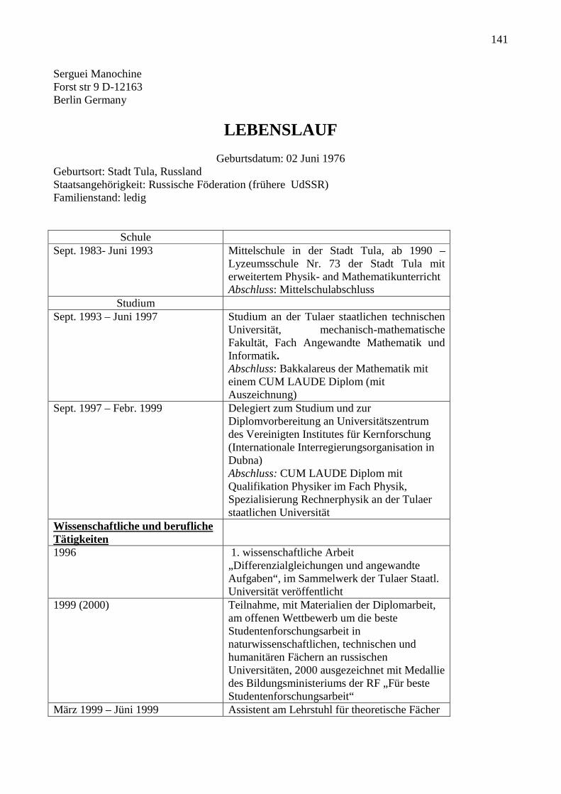
141

Serguei Manochine Forst str 9 D-12163 Berlin Germany

LEBENSLAUF

Geburtsdatum: 02 Juni 1976 Geburtsort: Stadt Tula, Russland Staatsangehörigkeit: Russische Föderation (frühere UdSSR) Familienstand: ledig

Schule Sept. 1983- Juni 1993 Mittelschule in der Stadt Tula, ab 1990 –

Lyzeumsschule Nr. 73 der Stadt Tula mit erweitertem Physik- and Mathematikunterricht Abschluss: Mittelschulabschluss

Studium Sept. 1993 – Juni 1997 Studium an der Tulaer staatlichen technischen

Universität, mechanisch-mathematische Fakultät, Fach Angewandte Mathematik und Informatik. Abschluss: Bakkalareus der Mathematik mit einem CUM LAUDE Diplom (mit Auszeichnung)

Sept. 1997 – Febr. 1999 Delegiert zum Studium und zur Diplomvorbereitung an Universitätszentrum des Vereinigten Institutes für Kernforschung (Internationale Interregierungsorganisation in Dubna) Abschluss: CUM LAUDE Diplom mit Qualifikation Physiker im Fach Physik, Spezialisierung Rechnerphysik an der Tulaer staatlichen Universität

Wissenschaftliche und berufliche Tätigkeiten

1996 1. wissenschaftliche Arbeit „Differenzialgleichungen und angewandte Aufgaben“, im Sammelwerk der Tulaer Staatl. Universität veröffentlicht

1999 (2000) Teilnahme, mit Materialien der Diplomarbeit, am offenen Wettbewerb um die beste Studentenforschungsarbeit in naturwissenschaftlichen, technischen und humanitären Fächern an russischen Universitäten, 2000 ausgezeichnet mit Medallie des Bildungsministeriums der RF „Für beste Studentenforschungsarbeit“

März 1999 – Jüni 1999 Assistent am Lehrstuhl für theoretische Fächer

142

der Fakultät für ausländische Studenten der Tulaer staatlichen Universität. Habe Physik unterrichtet.

Juni 1999- März 2002 Immatrikuliert in der Direktstudiumaspirantur (Vorbereitung der Nachwuchswissenschaftler) der Tulaer staatlichen Universität im Fach „Mechanik des deformierten Festkörpers“ und delegiert, ab November 1999, zur wissenschaftlichen Arbeit am Frank-Laboratorium für Neutronenphysik des Vereinigten Institutes für Kernforschung Dubna. Tätig in der Abteilung für Spektrometerkomplexe, unter wiss. Leitung des Abteilungleiters Dr. A.V. Belushkin. Vortäge im Abteilungsseminar, an der Konferenz junger Wissenschaftler des Institutes, Veröffentlichung von 4 wissenschaftlichen Arbeiten.

Jan. 2001 – April 2001 Gastwissenschaftler (guest scientist) am Hahn-Meitner-Institut, Projekt VITESS – Virtual Instrument Tool for ESS

März 2002 – bis heute Wissenschaftlicher angestellter (Doktorand) am Hahn-Meitener-Institut, Projekt VITESS. Tätig in der Abteilung „Methoden und Instrumente“, unter wiss. Leitung des Abteilungleiters Prof. Dr. F. Mezei, Veröffentlichung von 6 wissenschaftlichnen Arbeiten. Immatrikuliert in der Fakultät Mathematik und Naturwissenschaften der TU-Berlin in Fach „Physik“

Fremdsprachen English als Arbeitssprache, selbtsverständlich auch Russisch

Berlin, 06.03.2005 Serguei Manochine

143

Erklärung Ich versichere, dass ich meine Dissertation „ Neue Softwaretools für die Entwicklung von Neutronenstreuinstrumenten für zukünftige Neutronenquellen“ selbständig und ohne unerlaubte Hilfe angefertigt habe, und dass ich sie in der jetzigen oder in ähnlicher Form weder einer anderen Fakultät der Technischen Universität Berlin noch einer anderen Hochschule eingereicht habe. Hiermit bestätige ich, dass die zur Zeit geltende Promotionsordnung mir bekannt ist. Berlin, 06.03.2005 Serguei Manochine

144