Embed Size (px)
Citation preview
HAL Id: tel-00996061https://tel.archives-ouvertes.fr/tel-00996061
Submitted on 26 May 2014
HAL is a multi-disciplinary open accessarchive for the deposit and dissemination of sci-entific research documents, whether they are pub-lished or not. The documents may come fromteaching and research institutions in France orabroad, or from public or private research centers.
L’archive ouverte pluridisciplinaire HAL, estdestinée au dépôt et à la diffusion de documentsscientifiques de niveau recherche, publiés ou non,émanant des établissements d’enseignement et derecherche français ou étrangers, des laboratoirespublics ou privés.
New structure learning algorithms and evaluationmethods for large dynamic Bayesian networks
Ghada Trabelsi
To cite this version:Ghada Trabelsi. New structure learning algorithms and evaluation methods for large dynamic Bayesiannetworks. Machine Learning [cs.LG]. Université de Nantes; Ecole Nationale d’Ingénieurs de Sfax, 2013.English. �tel-00996061�
These de Doctorat
Ghada TRABELSIMemoire presente en vue de l’obtention du
grade de Docteur de l’Universite de Nantes
sous le label de l’Universite de Nantes Angers Le Mans
Discipline : InformatiqueLaboratoire : Laboratoire d’informatique de Nantes-Atlantique (LINA)REsearch Group on Intelligent Machines (REGIM)Ecole Nationale d’ingenieurs de Sfax, university of Sfax
Soutenue le 13 decembre 2013
Ecole doctorale : 503 (STIM)These n°:
New structure learning algorithms and
evaluation methods for large dynamic
Bayesian networks
JURY
Rapporteurs : Mme Nahla BEN AMOR, Professeur des Universites, University of Tunis
M. Ioannis TSAMARDINOS, Professeur des universites, Univerity of Crete
Examinateurs : M. Marc GELGON, Professeur des Universites, University of Nantes
M. Sylvain PIECHOWIAK, Professeur des Universites, University of Valenciennes et Hainaut-Cambresis
Invite : M. Mounir BEN AYED, Maıtre Assistant, University of Sfax
Directeur de these : M. Philippe LERAY, Professeur des universites, University of Nantes
Co-directeur de these : M. Adel. M. ALIMI, Professeur des Universites, University of Sfax

2
Declaration of originality: I hereby declare that this thesis is based on my own
work and has not been submitted for any other degree or professional qualification,
except when otherwise stated. Much of the work presented here has appeared in
previously published conference and workshop papers. The chapters discussing the
Benchmarking dynamic Bayesian Networks structure learning, DMMHC approach
and evaluating its performance on real data are based on [100, 101]. Where refer-
ence is made to the works of others, the extent to which that work has been used is
indicated and duly acknowledged in the text and bibliography.
Ghada TRABELSI BEN SAID (November, 2013)

DEDICATION
There are a number of people without whom this thesis might not have been
written, and to whom I am greatly indebted.
I would first like to express my gratitude to all members of the jury, Sylvain
PIECHOWIAK, Marc GELGON, Nahla BEN AMOR, Ioannis TSAMARDINOS
who consented to assess my thesis document.
I would like to thank my supervisor, Pr. Adel M. AlIMI, for his guidance and
support throughout this study. as well as my co-supervisor Dr. Mounir BEN AYED
who believed in me and provided me with beneficials comments and questions that
were vital for the completion of the thesis. I owe him a lot.
I have been very fortunate for having Pr. Philippe LERAY as my research advi-
sor. Many thanks to Pr. Leray for introducing me to an interesting research area and
inviting me to work in France, where my thesis was partially achieved. I would like
to express my heartfelt gratefulness for his guidance and support. I am really licky
to learn from the best. My collaboration with him has helped me grow not only as
a researcher but also as an individual.
I am indebted to Dr. Nahla BEN AMOR and Dr. Pierre-Henri WUILLEMIN
who kindly accepted to have interesting discussions with me as thesis monitoring
committee.
Special knowledgement to Dr. Amanullah YASIN, Dr. Hela LTIFI and PHD.
student Mouna BEN ISHAK for their generous support and help during the pro-
gramming and writing phases.
I would like to thank my parents deeply as they have supported me all the way
since the beginning of my studies. They have been understanding, infinitly loving
and provided me with their prayers that have been my greatest strength all these
years.
3

4
This thesis is dedicated also to my dear husband who has been a great source
of motivation and inspiration for me and I thank him for giving me new dreams to
pursue.
Finally, this thesis is dedicated to my sisters, friends, and colleagues for their
love, endless support and encouragement. It is dedicated to all those who believe in
the richness of learning.
Abbreviations and Acronyms
AIC Akaike Information Criterion
BIC Bayesian Information Criterion
BD Bayesian Dirichlet
BDe Bayesian Dirichlet Equivalent
BN Bayesian Network
CPC set of Parents Children candidates
CPCt set of Parents Children candidates in t time slice
CPt−1 set of Parent candidates in t-1 time slice
CPDAG Complete Partially Directed Acyclic Graph
CCt+1 set of Children candidates in t+1 time slice
DAG Directed Acyclic Graph
DBN Dynamic Bayesian Network
DMMHC Dynamic Max Min Hill Climbing
DMMPC Dynamic Max Min Parents Children
DSS Decision support System
EM Expectation Maximization
GS Greedy Search
G0 Initial network
G→ Transition network
HBN Hierarchical Bayesian Netxork
IC, PC Inductive/Predictive Causation
KDD knowledge Data Discovery
KL-divergence Kullback-Leibler divergence
MB Markov Blanket
MCMC Monte Carlo Markov Chain
MDL Minimum Description Length
MIT Mutual Information test
MMH Max Min Heuristic
MMHC Max Min Hill Climbing
MMPC Max Min Parents Children
5

6
MWST Maximum Weight Spanning Tree
Ne0 set of neigherbood in time slice 0
Ne+ set of neigherbood in time slice t ≥ 1
PDAG Partially Directed Acyclic Graph
PDAGk Partially Directed Acyclic Graph with knowledge
SA Simulated Annuling
SHD Structural hamming Distance
SHD(2-TBN) Structural hamming Distance for 2-TBN
SGS Spirtes, Glymour & Scheines
RB Reseau Bayesien
RBD Reseau Bayesien Dynamique
2-TBN two-slices Temporal Bayes Net

Resume
La plupart des techniques de fouille des donnees utilisent des algorithmes qui
fonctionnent sur des donnees fixes non temporelles. Cela est du a la difficulte de
la construction de ces modeles au niveau de l’exploitation des donnees temporelles
(que certains qualifient comme complexes) qui sont delicates a manipuler. Ainsi
peu des travaux proposent des algorithmes standards pour l’extraction des connais-
sances a partir de donnees multidimensionnelles et temporelles contrairement aux
donnees statiques.
Dans plusieurs domaines tels que celui de la sante les donnees concernant un in-
dividu sont saisies a des moments differents d’une maniere plus ou moins periodiques.
Ainsi, dans ce domaine le temps est un parametre important. Nous avons cherche a
simplifier cette dimension (le temps) en utilisant un ensemble de techniques complementaires
de fouilles des donnees.
Dans ce contexte, la presente these presente deux contributions : l’extraction des
modeles de connaissances en utilisant les reseaux bayesiens dynamiques (RBD)
comme etant une technique de fouille de donnees et l’evaluation de ces modeles
temporels (dynamiques).
L’apprentissage de structure dans les Reseaux Bayesiens (RB) est un probleme
d’optimisation combinatoire. En ce qui concerne la dependance temporelle, les
reseaux bayesiens sont changes par les reseaux bayesiens dynamiques. L’integration
du terme ” temporel ” rend l’apprentissage de structure dans les RBD plus com-
plique. Nous sommes ainsi obliges de chercher l’algorithme le plus adequat et le
plus rapide pour resoudre ce probleme.
Dans les developpements recents, les algorithmes d’apprentissage de structure
dans les modeles graphiques temporels bases sur les scores sont utilises par plusieurs
d’equipes de chercheurs dans le monde entier. Neanmoins, il existe quelques algo-
rithmes d’apprentissage de structure des RB qui incorporent la methode de recherche
locale qui permet un meilleur passage a l’echelle. Cette methode de recherche lo-
cale combine les algorithmes d’apprentissage bases sur les scores et ceux bases sur
les contraintes. Cette methode hybride, peut etre utile pour etre appliquer sur les
reseaux bayesiens dynamiques pour l’apprentissage de structure. Nous avons pu par
cette methodes de rendre l’apprentissage de structure dans les RBD plus pratique
et diminuer l’espace de recherche de solutions dans les RBD qui est qualifie par
7

8
sa complexite a cause de la temporalite. Nous avons aussi propose une approche
pour l’evaluation des modeles graphiques temporels (construits lors de l’etape de
l’apprentissage de structure).
L’apprentissage de structure pour les RB statiques est bien etudie par plusieurs
groupes de recherches. Nombreuses approches concernant ce sujet sont proposees
et l’evaluation de ses algorithmes se fait par l’utilisation des differents standards
Benchmarks et mesures d’evaluations.
A notre connaissance, toutes les etudes qui s’interessent a l’apprentissage de
structure pour les RBDs utilisent ses propres reseaux, techniques d’evaluations
et indicateurs de comparaison. Ainsi l’acces aux bases de donnees et aux codes
sources de ces algorithmes n’est pas toujours possible.
Pour resoudre ce probleme, nous avons propose une nouvelle approche pour la
generation des grands benchmarks standards pour les RBD. Cette approche se base
sur le Tiling avec une metrique permettant d’evaluer la performance des algorithmes
d’apprentissage de structure pour les RBDs de type 2-TBN.
Nous avons obtenu des resultats interessants. Le premier fournit un outil de
generation des larges benchmarks pour l’evaluation des reseaux bayesiens dynamique.
Le deuxieme, consiste a une nouvelle mesure pour evaluer la performance des algo-
rithmes d’apprentissage de structure. Comme troisieme resultat, nous avons montre
dans la partie experimentale que les algorithmes DMMHC developpes sont plus
perfermants que les autres algorithmes d’apprentissage de structure pour les RBDs
existants.
Abstract
Most of data mining techniques use algorithms that work on fixed non-temporal
data. This is due to the difficulty of the construction of these models in exploitating
temporal data (described as complex) which are difficult to handle. A small number
of works that proposed algorithms to extract knowledge from temporal and multi-
dimensional data differently from the static ones.
In many fields such as health, data about an individual are captured at different
times on a more or less regular basis. Thus, in this field, time is an important
parameter. Using a set of complementary data mining techniques, we tried to solve
this persisting problem.
In this context, this thesis presents two fundamental contributions: the extraction
of knowledge models using dynamic bayesian networks (DBNs) as a data mining
technique and techniques for the evaluation of these temporal (dynamic) models.
The structure learning in the bayesian networks (BNs) is a combinatorial op-
timization problem. Regarding the time dependence, the Bayesian networks are
changed by Dynamic Bayesian Networks (DBNs). The inclusion of the term ”Time”
makes the learning structure more complicated. We are thus obliged to seek for the
most appropriate algorithm and the fastest way to solve this problem.
In recent developments, the structure learning algorithms in temporal graphical
models based on the scores are used by many research teams around the world.
However, there are some BNs structure learning algorithms that incorporate local
search methods that provide a better scalability. This local search method is hy-
brid, i.e it combines the learning algorithms based on the scores and the learning
algorithms based on constraints. This method can be useful to be applied to the Dy-
namic Bayesian Networks for learning structure. Relying on this method we tried
to make the learning structure of DBNs more convenient and reduce its complexity
caused by temporality.
The other problem that arises is the evaluation of these temporal graphical mod-
els (built by the structure learning step). The structure learning for static BN has
been well studied by several research groups. Many approaches have been proposed
on this topic. The evaluation of their algorithms is done by the use of different stan-
dards Benchmarks and evaluation measures.
As far as we know, all studies on DBNs structure learning use their own net-
9

10
works and indicators of comparison. In addition, the access to the datasets and to
the source code is not always possible. To solve this problem, we proposed a new
approach for the generation of large standard benchmarks for DBNs which is based
on the Tiling with a metric used to evaluate the performance of structure learning
algorithms for DBNs (2-TBN).
We obtained interesting results, first we provided a tool for benchmarking dy-
namic Bayesian network structure learning algorithms. Second, we proposed a
novel metric for evaluating the structure learning algorithms performance. As a
third result, we showed in the experimental results that the DMMHC algorithms
achieve better performance than the other existing structure learning for DBNs.
Contents
1 Introduction 19
1.1 Research context . . . . . . . . . . . . . . . . . . . . . . . . . . . 20
1.2 Thesis overview . . . . . . . . . . . . . . . . . . . . . . . . . . . . 22
1.3 Publications . . . . . . . . . . . . . . . . . . . . . . . . . . . . . . 23
I State of the art 25
2 Bayesian Network and structure learning 27
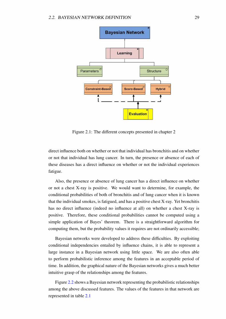
2.1 Introduction . . . . . . . . . . . . . . . . . . . . . . . . . . . . . . 28
2.2 Bayesian Network definition . . . . . . . . . . . . . . . . . . . . . 28
2.2.1 Description example [75] . . . . . . . . . . . . . . . . . . . 28
2.2.2 Basic concepts . . . . . . . . . . . . . . . . . . . . . . . . 30
2.2.3 Bayesian Network definition . . . . . . . . . . . . . . . . . 32
2.2.4 Markov equivalence classes for directed Acyclic Graphs . . 33
2.3 Bayesian network structure learning . . . . . . . . . . . . . . . . . 35
2.3.1 Constraint-Based Learning . . . . . . . . . . . . . . . . . . 36
2.3.2 Score-Based Learning . . . . . . . . . . . . . . . . . . . . 37
2.3.3 Hybrid method or local search . . . . . . . . . . . . . . . . 39
2.3.4 Learning with large number of variables . . . . . . . . . . . 41
2.4 Evaluation of Bayesian Network structure learning algorithms . . . 42
2.4.1 Evaluation metrics . . . . . . . . . . . . . . . . . . . . . . 42
2.4.2 Generating large Benchmarks . . . . . . . . . . . . . . . . 45
2.5 Conclusion . . . . . . . . . . . . . . . . . . . . . . . . . . . . . . 46
3 Dynamic Bayesian Networks and structure learning 49
3.1 Introduction . . . . . . . . . . . . . . . . . . . . . . . . . . . . . . 50
3.2 Dynamic Bayesian Network Definition . . . . . . . . . . . . . . . . 50
3.2.1 Representation . . . . . . . . . . . . . . . . . . . . . . . . 50
3.2.2 Different forms of K-TBN . . . . . . . . . . . . . . . . . . 51
3.3 Dynamic Bayesian Network structure learning . . . . . . . . . . . . 55
3.3.1 Principle . . . . . . . . . . . . . . . . . . . . . . . . . . . 55
11
12 CONTENTS
3.3.2 Structure learning approaches for 2-TBN and k-TBN models 55
3.3.3 Structure learning approaches for simplified ”k-TBN and
2-TBN” models . . . . . . . . . . . . . . . . . . . . . . . . 56
3.3.4 Structure learning approaches for other forms of DBN models 57
3.4 Evaluation of DBN structure learning algorithms . . . . . . . . . . 58
3.4.1 Benchmarks . . . . . . . . . . . . . . . . . . . . . . . . . . 58
3.4.2 Evaluation metric . . . . . . . . . . . . . . . . . . . . . . . 59
3.5 Conclusion . . . . . . . . . . . . . . . . . . . . . . . . . . . . . . 60
II Contributions 63
4 Benchmarking dynamic Bayesian networks 65
4.1 Introduction . . . . . . . . . . . . . . . . . . . . . . . . . . . . . . 66
4.2 Generation of large k-TBN and simplified k-TBN . . . . . . . . . . 67
4.2.1 Principle . . . . . . . . . . . . . . . . . . . . . . . . . . . 67
4.2.2 Tiling the initial model . . . . . . . . . . . . . . . . . . . . 67
4.2.3 Tiling the transition model . . . . . . . . . . . . . . . . . . 68
4.3 Evaluation of k-TBN generated by data and prior knowledge . . . . 69
4.3.1 Principle . . . . . . . . . . . . . . . . . . . . . . . . . . . 69
4.4 Validation examples . . . . . . . . . . . . . . . . . . . . . . . . . . 72
4.4.1 2-TBN Benchmark generation . . . . . . . . . . . . . . . . 72
4.4.2 SHD for 2-TBN . . . . . . . . . . . . . . . . . . . . . . . . 74
4.5 Conclusion . . . . . . . . . . . . . . . . . . . . . . . . . . . . . . 75
5 Dynamic Max Min Hill Climbing (DMMHC) 77
5.1 Introduction . . . . . . . . . . . . . . . . . . . . . . . . . . . . . . 79
5.2 Dynamic Max Min Parents and children DMMPC . . . . . . . . . . 79
5.2.1 Naıve DMMPC (neighborhood identification) . . . . . . . 80
5.2.2 Optimized DMMPC (Neighborhood identification) . . . . . 81
5.2.3 Toy example (naive DMMPC vs optimised DMMPC) . . . 83
5.2.4 Symmetrical correction . . . . . . . . . . . . . . . . . . . . 84
5.3 Dynamic Max Min Hill-Climbing DMMHC . . . . . . . . . . . . . 85
5.4 DMMHC for simplified 2-TBN . . . . . . . . . . . . . . . . . . . . 87
5.5 Time complexity of the algorithms . . . . . . . . . . . . . . . . . . 88
5.6 Related work . . . . . . . . . . . . . . . . . . . . . . . . . . . . . 90
5.7 Conclusion . . . . . . . . . . . . . . . . . . . . . . . . . . . . . . 90
6 Experimental study 95
6.1 Introduction . . . . . . . . . . . . . . . . . . . . . . . . . . . . . . 96
6.2 Experimental protocol . . . . . . . . . . . . . . . . . . . . . . . . 96
CONTENTS 13
6.2.1 Algorithms . . . . . . . . . . . . . . . . . . . . . . . . . . 96
6.2.2 Benchmarks . . . . . . . . . . . . . . . . . . . . . . . . . . 97
6.2.3 Performance indicators . . . . . . . . . . . . . . . . . . . . 97
6.3 Empirical results and interpretations on complete search space . . . 98
6.3.1 Initial validation . . . . . . . . . . . . . . . . . . . . . . . 98
6.3.2 DMMHC versus dynamic GS and SA . . . . . . . . . . . . 99
6.3.3 Naive versus optimized DMMHC . . . . . . . . . . . . . . 102
6.4 Empirical results and interpretations on simplified search space . . . 104
6.4.1 Simplified 2-TBN with small benchmark . . . . . . . . . . 104
6.4.2 Simplified 2-TBN with large benchmark . . . . . . . . . . . 107
6.5 Comparison between all DMMHC versions . . . . . . . . . . . . . 108
6.6 Conclusion . . . . . . . . . . . . . . . . . . . . . . . . . . . . . . 110
7 Conclusion 111
7.1 Summary . . . . . . . . . . . . . . . . . . . . . . . . . . . . . . . 112
7.2 Applications . . . . . . . . . . . . . . . . . . . . . . . . . . . . . . 113
7.3 Limitations . . . . . . . . . . . . . . . . . . . . . . . . . . . . . . 114
7.4 Issues for future researches . . . . . . . . . . . . . . . . . . . . . . 115
A Bayesian Network and Parameter learning 117
A.1 From completed data . . . . . . . . . . . . . . . . . . . . . . . . . 117
A.1.1 Statistical Learning . . . . . . . . . . . . . . . . . . . . . . 117
A.1.2 Bayesian Learning . . . . . . . . . . . . . . . . . . . . . . 118
A.2 From incomplete data . . . . . . . . . . . . . . . . . . . . . . . . . 118
A.2.1 Nature of the missing data and their treatment . . . . . . . . 118
A.2.2 EM algorithm . . . . . . . . . . . . . . . . . . . . . . . . . 119
B Benchmarking the dynamic bayesian network 121
B.1 BNtiling for 2-TBN implementation . . . . . . . . . . . . . . . . . 121
B.2 Generating large Dynamic Bayesian Networks . . . . . . . . . . . . 122
C DMMHC: Dynamic Max Min Hill Climbing 123
C.1 Proofs of propositions used by DMMHC . . . . . . . . . . . . . . . 123
C.1.1 Proof proposition 5.2.2: . . . . . . . . . . . . . . . . . . . 123
C.1.2 Proof proposition 5.4.1: . . . . . . . . . . . . . . . . . . . 125

List of Tables
2.1 The values of the features . . . . . . . . . . . . . . . . . . . . . . . 30
4.1 Generated benchmarks for Dynamic Bayesian Network . . . . . . . 73
6.1 Characteristics of 2T-BNs (G0, G�) generated from 6 usual static
BNs (Asia, Alarm, Hailfinder, Win95pts, Andes, Link) . . . . . . . 97
6.2 SHD comparison with existing static structure learning approaches
([34],[22]), for Alarm, Hailfinder and Link benchmarks with 5000
samples. . . . . . . . . . . . . . . . . . . . . . . . . . . . . . . . . 98
6.3 Average±standard deviation of SHD obtained by GS and DMMHC
in G0 . . . . . . . . . . . . . . . . . . . . . . . . . . . . . . . . . . 99
6.4 Average±standard deviation of SHD obtained by GS and DMMHC
in G� . . . . . . . . . . . . . . . . . . . . . . . . . . . . . . . . . 100
6.5 Average±standard deviation running time for DMMHC and GS in G0 100
6.6 Average±standard deviation running time for DMMHC and GS in G�100
6.7 Average±standard deviation of SHD obtained by SA and DMMHC
in G� . . . . . . . . . . . . . . . . . . . . . . . . . . . . . . . . . 101
6.8 Average±standard deviation SHD for naive and optimised DMMHC
in G� . . . . . . . . . . . . . . . . . . . . . . . . . . . . . . . . . 103
6.9 Average±standard deviation running time for naive and optimised
DMMHC in G� . . . . . . . . . . . . . . . . . . . . . . . . . . . . 103
15

List of Figures
1.1 Thesis overview and interdependencies between chapters . . . . . . 22
2.1 The different concepts presented in chapter 2 . . . . . . . . . . . . 29
2.2 Example of Bayesian Network . . . . . . . . . . . . . . . . . . . . 30
2.3 Patterns for paths through a node . . . . . . . . . . . . . . . . . . . 32
2.4 (a) Example of DAG, (b) the skeleton relative to the DAG and (c)
an example of a PDAG [70] . . . . . . . . . . . . . . . . . . . . . . 34
2.5 Orientation rules for patterns [69] . . . . . . . . . . . . . . . . . . 35
3.1 A structure of 2-TBN Bayesian network . . . . . . . . . . . . . . . 51
3.2 An example of 2-TBN Bayesian network [110] . . . . . . . . . . . 52
3.3 An example of k-TBN visualization of a second-order DBN (k=3)
using t = 3 time-slices . . . . . . . . . . . . . . . . . . . . . . . . . 53
3.4 Simplified k-TBN . . . . . . . . . . . . . . . . . . . . . . . . . . . 54
4.1 An example output of the initial model generation algorithm. The
generating network is ASIA benchmark [59] shown in the top left
of the figure. . . . . . . . . . . . . . . . . . . . . . . . . . . . . . . 68
4.2 An example output of the 2-TBN generation algorithm. The gener-
ating network is ASIA benchmark [59] shown in the top left of fig-
ure a). a) The output of the initial network consists of three tiles of
Asia with the addition of several intraconnecting edges shown with
the dashed edges. b) The transition network output together with
several added interconnecting edges are shown with the dashed red
edges. . . . . . . . . . . . . . . . . . . . . . . . . . . . . . . . . . 73
4.3 Examples of structural Hamming distance with or without temporal cor-
rection. A first 2-TBN and its corresponding PDAG and corrected PDAG k
are shown in (a). (b) and (c) show another 2-TBN and their corresponding
PDAG, and the structural Hamming distance with the first model . . . . . 75
5.1 Conditional dependence. (a) divergence case. (b) convergence case . . . 82
5.2 The extended Umbrella DBN . . . . . . . . . . . . . . . . . . . . . 83
5.3 Example trace of naive DMMPC . . . . . . . . . . . . . . . . . . . 85
17
18 LIST OF FIGURES
5.4 Example trace of optimised DMMPC . . . . . . . . . . . . . . . . 86
5.5 Example trace of simplified DMMPC . . . . . . . . . . . . . . . . 88
6.1 Average SHD vs running time obtained by GS and DMMHC with
respect to sample size in initial graph . . . . . . . . . . . . . . . . . 101
6.2 Average SHD(DMMHC) vs SHD(GS) with respect to sample size
in transition graph . . . . . . . . . . . . . . . . . . . . . . . . . . . 101
6.3 Average SHD(DMMHC) vs SHD(SA) with respect to sample size
in transition graph . . . . . . . . . . . . . . . . . . . . . . . . . . . 102
6.4 Average SHD vs running time obtained by naive and optimised
DMMHC with respect to sample size in transition graph . . . . . . 104
6.5 Network reconstruction results for GS algorithm of Banjo tool. The
used benchmark is the biological dataset 20 variables and 2000 ob-
servations . . . . . . . . . . . . . . . . . . . . . . . . . . . . . . . 105
6.6 Network reconstruction results for simplified 2-TBN DMMHC. The
used benchmark is the biological dataset 20 variables and 2000 ob-
servations. . . . . . . . . . . . . . . . . . . . . . . . . . . . . . . . 106
6.7 Network reconstruction results for MIT-based global, MIT-based
MMMB, Banjo [110] and DMMHC from Cyanothece genetic bench-
marks . . . . . . . . . . . . . . . . . . . . . . . . . . . . . . . . . 108
6.8 Network reconstruction results . . . . . . . . . . . . . . . . . . . . 109
6.9 Complexity of all DMMHC versions . . . . . . . . . . . . . . . . . 110
A.1 Example of BN structure . . . . . . . . . . . . . . . . . . . . . . . 118

1Introduction
Sommaire
1.1 Research context . . . . . . . . . . . . . . . . . . . . . . . . . 20
1.2 Thesis overview . . . . . . . . . . . . . . . . . . . . . . . . . 22
1.3 Publications . . . . . . . . . . . . . . . . . . . . . . . . . . . 23
19
20 CHAPTER 1. INTRODUCTION
1.1 Research context
Time is an important factor in several domains as medicine, finance and indus-
try. It is one of the important problems in machine learning. Machine Learning
is the study of methods for programming computers to learn. Computers are used
to perform a wide range of tasks, and for most of these it is relatively easy for
programmers to design and implement the necessary software. However, there are
many tasks for which this is difficult or impossible. These can be divided into four
general categories.
– Tasks for which there exist no human experts.
– Tasks where human experts exist, but where they are unable to explain their
expertise.
– Tasks with rapidly-changing phenomena.
– Tasks where applications that need to be customized for each user separately.
Machine learning addresses many of the same research questions as the fields
of statistics, data mining, but with differences of emphasis. Statistics focuses on
understanding the phenomena that have generated the data, often with the goal of
testing different hypotheses about those phenomena. Data mining seeks to find pat-
terns in the data that are understandable by people [26].
Most of studies use data mining techniques for the training of fixed data and the
extraction of the static knowledge models. Among these models we find the prob-
abilistic graphical model, commonly used in probability theory, statistics, Bayesian
statistics and machine learning.
Graphical models are a marriage between probability theory and graph theory.
They provide a natural tool for dealing with two problems that occur throughout
applied mathematics and engineering, uncertainty and complexity, and in partic-
ular they are playing an increasingly important role in the design and analysis of
machine learning algorithms. Fundamental to the idea of a graphical model is the
notion of modularity, a complex system is built by combining simpler parts. Prob-
ability theory provides the glue whereby the parts are combined, ensuring that the
system as a whole is consistent, and providing ways to interface models to data.
The graph theoretic side of graphical models provides both an intuitively appealing
interface by which humans can model highly-interacting sets of variables as well as
a data structure that lends itself naturally to the design of efficient general-purpose
algorithms [32].
Bayesian networks [78, 48, 52] are a kind of the probabilistic graphical models.
They are frequently used in the field of Knowledge from Data Discovery (KDD).
A Bayesian network is a directed acyclic graph whose nodes represent variables
and directed arcs denote statistical dependence relations between variables, and a
probability distribution is specified over these variables. Dynamic systems model-
1.1. RESEARCH CONTEXT 21
ing has resulted an extension of the BN called Dynamic Bayesian networks (DBN)
[23, 73]. In order to exploit relational models from time-series data (called discov-
ery task), it is natural to use a dynamic Bayesian network (DBN). DBN is a directed
graphical model whose nodes are across different time slices, to learn and reason
dynamic systems. DBNs model a temporal process using a conditional probability
distribution for each node and a probabilistic transition between time slices [113].
Learning a BN from observational data is an important problem that has been
studied extensively during the last decade. The construction of these models can
be acheieved either by using expertise, or from data. Many studies have been con-
ducted on this topic, leading to different approaches:
– Methods for the discovery of conditional independence in the data to recon-
struct the graph
– Methods for optimizing an objective function called score
– Methods for the discovery of local structure around a target variable to recon-
struct the global structure of the network
Most of the studies have been limited to the structure learning of Bayesian net-
works in the static cases. There are a few algorithms for DBN structure learning
[35, 50]. Most of these algorithms use a conventional method based on scores. In-
deed, the addition of the time dimension further complicated the search space of
solutions.
In the remainder of this thesis, we focus on the interest of hybrid approaches
(the local search identification and global optimisation) in the dynamic case, which
could more easily take into account the temporal dimension of our models.
Moreover, we noticed that the static BN structure learning is a well-studied do-
main. Many approaches have been proposed and the quality of these algorithms has
been studied over a range of different standard networks and methods of evaluation.
To our knowledge, all studies about DBN structure learning use their own bench-
marks and techniques for evaluation. The problem in the dynamic case is that we
don’t find previous works that provide details about used networks and indicators
of comparison. In addition, access to the datasets and the source code is not always
possible. In this thesis, we also focus on solving the evaluation problem in dynamic
case.
Our contribution consists to answer these issues:
1. Can we prove that the hybrid learning allows scaling in the dynamic case?
2. How can we evaluate this approach to justify the efficiency and scalability of
our approch?
22 CHAPTER 1. INTRODUCTION
1.2 Thesis overview
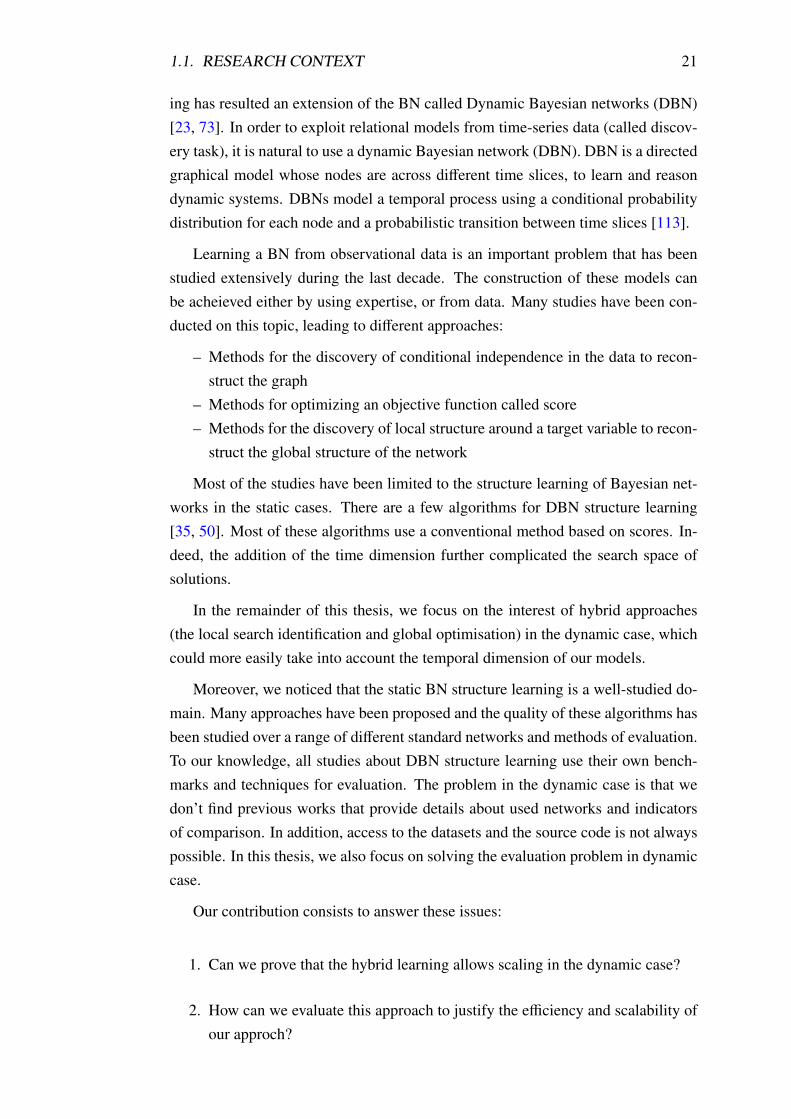
The structure of the thesis is organized around three intertwined topics, see Fig-
ure 1.1.
Figure 1.1: Thesis overview and interdependencies between chapters
Chapters 2 and 3 review the scientific background and establish the terminology
required to discuss the structure learning for Bayesian Networks, thus providing the
basis for the subsequent chapters of this thesis. It starts off by reminding some of
the basic notations and definitions that are commonly used in the Bayesian Network
literature.
Moreover, In chapter 3, we present the difference between the static Bayesian
networks and their extension called dynamic bayesian networks when the time di-
mension is added. The two chapters are end up with an overview of the existing
approaches for benchmarking static and dynamic bayesian networks and evaluating
the structure learning algorithms in literature.
1.3. PUBLICATIONS 23
Chapter 4 is dedicated for our contributions. Initially, we show a description of
our Benchmarking algorithms. The first one generates large dynamic bayesian with
(2-TBN) form. The second is an extension of the structural hamming distance al-
gorithm for the evaluation in the dynamic case. We also provide some experimental
validation to justify the performance and utility of our first contributions.
Chapter 5 describes our new algorithm for DBN structure learning based on
hybrid method. In this chapter, we give three (naıve, optimized and simplified)
versions of our algorithm with the different necessary demonstrations. The chapter
ends with the Time complexity of the algorithms and a toy example that presents
the construction of structure learning proposed by our algorithms applied on simple
Network.
Chapter 6 gives the different experiments achieved to show the performance of
DMMHC algorithm in many levels as the quality and computational complexity of
the algorithm for learning structure. In this chapter, we present the experimental
protocol used in this thesis project. After that, we try to represent the obtained
results and to compare the results given by the GS and SA algorithms with those
given by naıve and optimized versions of our DMMHC. Also an interpretation and
discussion of these results are achieved. In addition, we present a comparaison
between our simplified DMMHC and the structure learning algorithms applied on
a reduced search speace (2-TBN without intra-slice edges). Additional evidence of
the scalability of DMMHC is found in the final section of this chapter.
Chapter 7 concludes the thesis summarizing the major results that we obtained.
In addition, we tried to identify some perspectives for future research.
1.3 Publications
The following parts of this work have previously been published in different
international journals and conferences:
– The contribution presented in chapter 4 was summarized in an article pub-
lished in the proceedings of ICMSAO 2013 conference [100].
– The contribution presented in chapter 5 was summarized in an article pub-
lished in the proceedings of IDA 2013 conference [101].
– Other application contributions not described in this thesis, were made by our
research group in REGIM lab (Tunisia), have been the object of two scientific
publications in Data Mining Workshops (ICDMW), 2012 IEEE 12th Interna-
tional Conference [63] and International Journal of Advanced Research in
Artificial Intelligence [64]. In these works, we discussed the use of different
data mining techniques as the dynamic Bayesian Networks and 3D visualiza-
tion in Dynamic Medical Decision Support System.


I
State of the art
25


2Bayesian Network and structure
learning
Sommaire
2.1 Introduction . . . . . . . . . . . . . . . . . . . . . . . . . . . 28
2.2 Bayesian Network definition . . . . . . . . . . . . . . . . . . 28
2.2.1 Description example [75] . . . . . . . . . . . . . . . . . 28
2.2.2 Basic concepts . . . . . . . . . . . . . . . . . . . . . . 30
2.2.3 Bayesian Network definition . . . . . . . . . . . . . . . 32
2.2.4 Markov equivalence classes for directed Acyclic Graphs 33
2.3 Bayesian network structure learning . . . . . . . . . . . . . . 35
2.3.1 Constraint-Based Learning . . . . . . . . . . . . . . . . 36
2.3.2 Score-Based Learning . . . . . . . . . . . . . . . . . . 37
Greedy search algorithm . . . . . . . . . . . . . 38
Simulated annealing algorithm (SA) . . . . . . . 39
2.3.3 Hybrid method or local search . . . . . . . . . . . . . . 39
2.3.4 Learning with large number of variables . . . . . . . . . 41
2.4 Evaluation of Bayesian Network structure learning algorithms 42
2.4.1 Evaluation metrics . . . . . . . . . . . . . . . . . . . . 42
Score-based method . . . . . . . . . . . . . . . . . . . 43
Kullback-Leibler divergence-based method . . . . . . . 43
Sensitivity and specificity-based method . . . . . . . . . 44
Distance-based method . . . . . . . . . . . . . . . . . . 44
2.4.2 Generating large Benchmarks . . . . . . . . . . . . . . 45
27
28 CHAPTER 2. BAYESIAN NETWORK AND STRUCTURE LEARNING
2.5 Conclusion . . . . . . . . . . . . . . . . . . . . . . . . . . . . 46
2.1 Introduction
Knowledge representation and reasoning from these representations have given
birth for many models. Probabilistic graphical models, and more specifically the
Bayesian networks, initiated by Judea Pearl in the 1980s, have proven to be useful
tools for the representation of uncertain knowledge, and reasoning from incomplete
information. Afterwards many studies such as [78, 59, 49, 52] introduced Bayesian
probabilistic reasoning formalism.
In this thesis we are interested in Bayesian network learning. Learning Bayesian
network consists of two phases: parameter learning and structure learning. There
are three types of approaches for the structure learning: methods based on identi-
fication of conditional indepedence, methods based on the optimization of a score
and hybrid methods (cf. Figure 2.1).
To hightlight the benefits of structure learning algorithms, we have to evaluate
the quality of the Bayesian networks obtained by these learning algorithms. Many
evaluation metrics are used in research. Some of them are characterized by the use
of data as the score-based method. Some others are characterized by the use of a
reference model. In our context, we are interested in the evaluation techniques using
a reference model with a large number of variables.
This chapter reviews basic definitions and notations of classical Bayesian net-
work and conditional independence. Section 2.2 introduces some notations and
definitions of BN. Section 2.3 provides an overview of the static Bayesian networks
structure learning. Based on this background, Section 2.4 is devoted to the evalution
of Bayesian networks structure. Finally, in this chapter we present the existing ap-
proaches used to evaluate these structure learning algorithms on large benchmarks.
2.2 Bayesian Network definition
2.2.1 Description example [75]
The presence or absence of a disease in a human being has a direct influence on
whether a test for that disease turns out positive or negative. We would use Bayes’
theorem (cf. theorem 2.2.1) to compute the conditional probability of an individual
to have a disease when a test for the diseaseturns out to be positive.
Let’s consider the situation where several features are related through inference
chains. For example, whether or not an individual has a history of smoking has a
2.2. BAYESIAN NETWORK DEFINITION 29
Figure 2.1: The different concepts presented in chapter 2
direct influence both on whether or not that individual has bronchitis and on whether
or not that individual has lung cancer. In turn, the presence or absence of each of
these diseases has a direct influence on whether or not the individual experiences
fatigue.
Also, the presence or absence of lung cancer has a direct influence on whether
or not a chest X-ray is positive. We would want to determine, for example, the
conditional probabilities of both of bronchitis and of lung cancer when it is known
that the individual smokes, is fatigued, and has a positive chest X-ray. Yet bronchitis
has no direct influence (indeed no influence at all) on whether a chest X-ray is
positive. Therefore, these conditional probabilities cannot be computed using a
simple application of Bayes’ theorem. There is a straightforward algorithm for
computing them, but the probability values it requires are not ordinarily accessible;
Bayesian networks were developed to address these difficulties. By exploiting
conditional independencies entailed by influence chains, it is able to represent a
large instance in a Bayesian network using little space. We are also often able
to perform probabilistic inference among the features in an acceptable period of
time. In addition, the graphical nature of the Bayesian networks gives a much better
intuitive grasp of the relationships among the features.
Figure 2.2 shows a Bayesian network representing the probabilistic relationships
among the above discussed features. The values of the features in that network are
represented in table 2.1
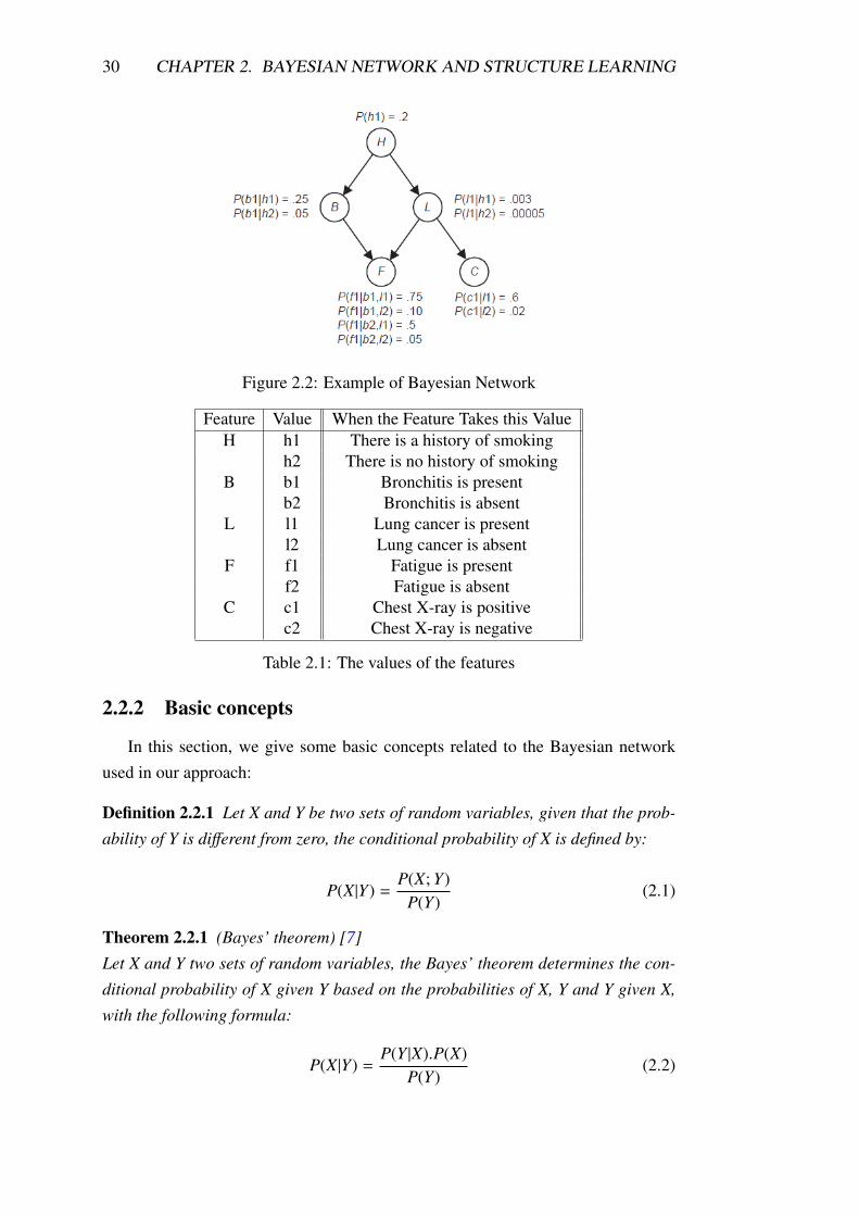
30 CHAPTER 2. BAYESIAN NETWORK AND STRUCTURE LEARNING
Figure 2.2: Example of Bayesian Network
Feature Value When the Feature Takes this Value
H h1 There is a history of smoking
h2 There is no history of smoking
B b1 Bronchitis is present
b2 Bronchitis is absent
L l1 Lung cancer is present
l2 Lung cancer is absent
F f1 Fatigue is present
f2 Fatigue is absent
C c1 Chest X-ray is positive
c2 Chest X-ray is negative
Table 2.1: The values of the features
2.2.2 Basic concepts
In this section, we give some basic concepts related to the Bayesian network
used in our approach:
Definition 2.2.1 Let X and Y be two sets of random variables, given that the prob-
ability of Y is different from zero, the conditional probability of X is defined by:
P(X|Y) =P(X; Y)
P(Y)(2.1)
Theorem 2.2.1 (Bayes’ theorem) [7]
Let X and Y two sets of random variables, the Bayes’ theorem determines the con-
ditional probability of X given Y based on the probabilities of X, Y and Y given X,
with the following formula:
P(X|Y) =P(Y |X).P(X)
P(Y)(2.2)
2.2. BAYESIAN NETWORK DEFINITION 31
Definition 2.2.2 (Independence)
Let X and Y two sets of random variables, X and Y are independent, denoted
≺X⊥Y≻, if and only if P(X|Y) = P (X).
Definition 2.2.3 (Conditionally independent)
Let X, Y, and Z be any three subsets of random variables. X and Y are said to be
conditionally independent given Z (noted IndP(X;Y | Z)) if P(X \ Y, Z) = P(X \ Z)
whenever P( Y,Z) ≻ 0.
Definition 2.2.4 (directed graph)
A directed graph G can be defined as an ordered pair that consists of a finite set V
of nodes and an irreflexive adjacency relation E on V. The graph G is denoted as
(V,E) . For each (x,y)∈ E we say that there is an arc (directed edge) from node x to
node y. In the graph, this is denoted by an arrow from x to y and x and y are called
the start point and the end point of the arrow respectively. We also say that node x
and node y are adjacent or x and y are neighbors of each other and node y and node
x are adjacent or y and x are neighbors of each other. x is also called a parent of y
and y is called a child of x. By using the concepts of parent and child recursively,
we can also define the concept of ancestor and descendent. We also call a node that
does not have any parent a root node. By irreflexive adjacency relation we mean
that for any x∈V , (x,x)< E , i.e., an arc cannot have a node as both its start point
and end point.
Definition 2.2.5 (Path)
A path in a directed graph is a sequence of nodes from one node to another using
the arcs.
Definition 2.2.6 (directed path and cycle)
A directed path from X1 to Xn in a DAG G is a sequence of directed edges X1�X2...
�Xn. The directed path is a cycle if X1=Xn (i.e. it begins and ends at the same
variable).
Definition 2.2.7 (A directed acyclic graph)
A DAG is a Directed Acyclic (without cycles) Graph (See Figure 2.4.a).
Definition 2.2.8 (d-separation)
Let S be a trail (that is, a collection of edges which is like a path, but each of whose
edges may have any direction) from node u to v. Then S is said to be d-separated by
a set of nodes Z if and only if (at least) one of the following holds:
1. S contains a chain, x � m � y, such that the middle node m is in Z,
2. S contains a fork, x � m � y, such that the middle node m is in Z, or
32 CHAPTER 2. BAYESIAN NETWORK AND STRUCTURE LEARNING
Figure 2.3: Patterns for paths through a node
3. S contains an inverted fork (or collider), x � m � y, such that the middle node
m is not in Z and no descendant of m is in Z.
The graph patterns of ”tail-to-tail”, ”tail-to-head” and ”head-to-head” are shown
in Figure 2.3. Thus u and v are said to be d-separated by Z if all trails between them
are d-separated. If u and v are not d-separated, they are called d-connected.
Definition 2.2.9 (D-separation for two sets of variables)
Two sets of variables X and Y are d-separated by Z in a graph G (noted DsepG(X;Y
\ Z)) if and only if ∀ u ∈ X and ∀ v ∈ Y, every tail from u to v d-separated by Z.
2.2.3 Bayesian Network definition
Definition 2.2.10 (Markov condition) [78]
The Markov condition can be stated as follows: Each variable Xi is conditionally
independent of all its no-descending, knowing the state of his parents, Pa(Xi).
IndP(Xi; NoDesc(Xi) \ Pa(Xi)). (2.3)
P(Xi|Pa(Xi); NoDesc(Xi)) = P(Xi|Pa(Xi)) (2.4)
Definition 2.2.11 (Bayesian Network) [75]
Let P be a joint probability distribution of the random variables in some set V, and
G = (V, E) be a DAG. We call (G,P) a Bayesian network if (G,P) satisfies the Markov
condition. P is the product of its conditional distributions in G, and this is the way
P is always represented in a Bayesian network.
A Bayesian Network B=(G,θ) is defined by:
– G=(V,E) directed graph without circuit whose vertices are associated with a
set of random variables X = X1,...,Xn, there is a bijection between X and V (i.e.
Xi←→Vi) and E is the set of arcs representing the conditional independence
between variables,
– θ = P(Xi|Pa(Xi)), all probabilities of each node Xi conditional on the state of
its parents Pa(Xi) in G.
2.2. BAYESIAN NETWORK DEFINITION 33
Pearl et al. [78] have also shown that the Bayesian networks allow us to represent
compactly the joint probability distribution over all variables:
P(X1, X2, ..., Xn) =
n∏
i=1
P(Xi|Pa(Xi)) (2.5)
This decomposition of a global function, into a product of local terms depending
only on the same node and its parents in the graph, is a fundamental property of
Bayesian networks.
Theorem 2.2.2 [93]
In a BN, two nodes are d-separated by Z, they are also conditionally independent
by Z.
DsepG(X; T |Z) = IndP(X; T |Z) (2.6)
The graphical part of the Bayesian network indicates the dependencies (or inde-
pendence) between variables and provides a visual tool for knowledge representa-
tion to make it more comprehensible to its users. In addition, the use of probabilities
allows taking into account the uncertainty in quantifying the dependencies between
variables.
2.2.4 Markov equivalence classes for directed Acyclic Graphs
There may be many DAGs associated to BNs that determine the same depen-
dence model. Thus, the family of all DAGs with a given set of vertices is naturally
partitioned into Markov-equivalence classes, with each class being associated with
a unique independence model (See Figure 2.4.c).
Definition 2.2.12 (Markov Equivalence) [77, 75, 104]
Two DAGs G1 and G2 on the same set of nodes are Markov Equivalent if for every
three mutually disjoint subsets A, B, C j V, DespG1(A,B | C)⇔ DespG2(A,B | C).
Theorem 2.2.3 (Verma and Pearl, 1991) [109]
Two DAGs are equivalent if and only if they have the same skeleton and the same
V-structures.
Definition 2.2.13 (Patterns) [69]
The pattern for a partially directed graph G is the partially directed graph which
has the identical adjacencies as G and which has an oriented edge A → B if and
only if there is a vertex C < adj(A) such that A → B and C → B in G. Let pattern
(G) denote the pattern for G. A triple (A, B, C) is an unshielded collider in G if and
only if A → B, C → B and A is not adjacent to B (V-structure). It is easy to show
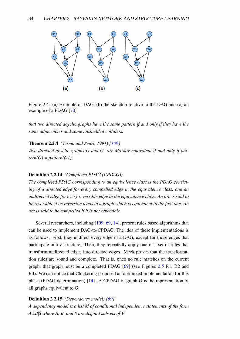
34 CHAPTER 2. BAYESIAN NETWORK AND STRUCTURE LEARNING
Figure 2.4: (a) Example of DAG, (b) the skeleton relative to the DAG and (c) an
example of a PDAG [70]
that two directed acyclic graphs have the same pattern if and only if they have the
same adjacencies and same unshielded colliders.
Theorem 2.2.4 (Verma and Pearl, 1991) [109]
Two directed acyclic graphs G and G’ are Markov equivalent if and only if pat-
tern(G) = pattern(G1).
Definition 2.2.14 (Completed PDAG (CPDAG))
The completed PDAG corresponding to an equivalence class is the PDAG consist-
ing of a directed edge for every compelled edge in the equivalence class, and an
undirected edge for every reversible edge in the equivalence class. An arc is said to
be reversible if its reversion leads to a graph which is equivalent to the first one. An
arc is said to be compelled if it is not reversible.
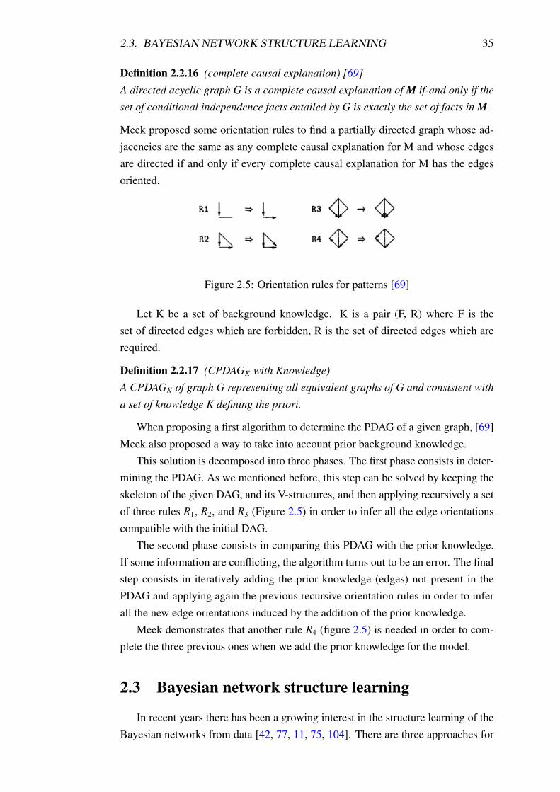
Several researchers, including [109, 69, 14], present rules based algorithms that
can be used to implement DAG-to-CPDAG. The idea of these implementations is
as follows. First, they undirect every edge in a DAG, except for those edges that
participate in a v-structure. Then, they repeatedly apply one of a set of rules that
transform undirected edges into directed edges. Meek proves that the transforma-
tion rules are sound and complete. That is, once no rule matches on the current
graph, that graph must be a completed PDAG [69] (see Figures 2.5 R1, R2 and
R3). We can notice that Chickering proposed an optimized implementation for this
phase (PDAG determination) [14]. A CPDAG of graph G is the representation of
all graphs equivalent to G.
Definition 2.2.15 (Dependency model) [69]
A dependency model is a list M of conditional independence statements of the form
A⊥B|S where A, B, and S are disjoint subsets of V
2.3. BAYESIAN NETWORK STRUCTURE LEARNING 35
Definition 2.2.16 (complete causal explanation) [69]
A directed acyclic graph G is a complete causal explanation of M if-and only if the
set of conditional independence facts entailed by G is exactly the set of facts in M.
Meek proposed some orientation rules to find a partially directed graph whose ad-
jacencies are the same as any complete causal explanation for M and whose edges
are directed if and only if every complete causal explanation for M has the edges
oriented.
Figure 2.5: Orientation rules for patterns [69]
Let K be a set of background knowledge. K is a pair (F, R) where F is the
set of directed edges which are forbidden, R is the set of directed edges which are
required.
Definition 2.2.17 (CPDAGK with Knowledge)
A CPDAGK of graph G representing all equivalent graphs of G and consistent with
a set of knowledge K defining the priori.
When proposing a first algorithm to determine the PDAG of a given graph, [69]
Meek also proposed a way to take into account prior background knowledge.
This solution is decomposed into three phases. The first phase consists in deter-
mining the PDAG. As we mentioned before, this step can be solved by keeping the
skeleton of the given DAG, and its V-structures, and then applying recursively a set
of three rules R1, R2, and R3 (Figure 2.5) in order to infer all the edge orientations
compatible with the initial DAG.
The second phase consists in comparing this PDAG with the prior knowledge.
If some information are conflicting, the algorithm turns out to be an error. The final
step consists in iteratively adding the prior knowledge (edges) not present in the
PDAG and applying again the previous recursive orientation rules in order to infer
all the new edge orientations induced by the addition of the prior knowledge.
Meek demonstrates that another rule R4 (figure 2.5) is needed in order to com-
plete the three previous ones when we add the prior knowledge for the model.
2.3 Bayesian network structure learning
In recent years there has been a growing interest in the structure learning of the
Bayesian networks from data [42, 77, 11, 75, 104]. There are three approaches for
36 CHAPTER 2. BAYESIAN NETWORK AND STRUCTURE LEARNING
finding a structure. The first approach poses learning as a constraint satisfaction
problem. In this approach, we try to identify the properties of conditional inde-
pendence among the variables in the data. This is usually done using a statistical
hypothesis test, like the χ2 test. We then build a network that exhibits the observed
dependencies and independencies.
The second approach poses learning as an optimization problem. We start by
defining a statistically motivated score that describes the fitness of each possible
structure from the observed data. The learner’s task is then to find a structure that
maximizes the score. In general, this is an NP-hard problem [11], and thus we
need to resort to heuristic methods. Although the constraint satisfaction approach is
efficient, it is sensitive to failures in independence tests. Thus, the common opinion
is that the optimization approach is a better tool for learning structure from a little
amount of data.
The third approach, named hybrid methods, can solve this problem by the com-
bination of the two previous ones. Local search methods are dealing with local
structure identification and global model optimization constrained with these local
information. These methods are able to scale distributions with more than thousands
of variables.
Generally, people face the problem of learning BNs from training data in order
to apply BNs to real-world applications. Typically, there are two categories in learn-
ing BNs, one is to learn BN parameters when a BN structure is known, and another
is to learn both BN structures and parameters. We notice that, learning BN param-
eters can be handled with complete and incomplete data. This kind of learning is
not as complicated as learning a BN structure. In this thesis, we focus on structure
learning with complete data, as we recommend to read appendix A before reading
this section.
2.3.1 Constraint-Based Learning
The idea of constraint-based structure learning is to know how to construct the
structure of Bayesian network if we can perform independence test (A ⊥ B|C).
Constraint-based methods employ the conditional independence tests to first
identify a set of conditional independence properties, and then attempts to iden-
tify the network structure that best satisfies these constraints corresponding to a
CPDAG.
Fast [29] describes the constraint identification as ”the process of learning the
skeleton and separating sets from the training data. Due to limited size of the train-
ing data, this process is inherently error-prone. The goal of constraint identification
is to efficiently identify the independence assertions while minimizing the number
of constraints that are inaccurate. Constraint identification algorithms appearing in
2.3. BAYESIAN NETWORK STRUCTURE LEARNING 37
the literature can be differentiated by three different design decisions: (1) the type of
independence test used, (2) the ordering heuristic and other algorithmic decisions,
and (3) the technique used to determine the reliability of the test”.
This first family of structure learning approaches for BN, often called search
under constraints, is derived from the work of Pearl’s team and Spirtes’ team. The
most popular constraint-based algorithms are IC [78], SGS and PC [77, 104] algo-
rithms. Three of them try to d-separate all the variable pairs with all the possible
conditional sets whose sizes are lower than a given threshold. They are based on
the same principle:
– build an undirected graph containing the relationships between variables, from
conditional independence tests
– detect the V-structures (also using conditional independence tests)
– propagate the orientation of some arcs with meek’s rules in section 2.2.4
– randomly direct some other edges in the graph without changing its CPDAG
– take into account the possible artificial causes due to latent variables.
One problem with constraint-based approaches is that they are difficult to reliably
identify the conditional independence properties and to optimize the network struc-
ture [67].
The constraint-based approaches lack an explicit objective function and they do
not try to directly find the global structure with maximum likelihood. So they do
not fit in the probabilistic framework.
This kind of approach rely on quite heavy assumptions such as the faithful-
ness and correctness of the independence tests. In contrast, score-based algorithms
search for the minimal model among all Bayesian networks.
2.3.2 Score-Based Learning
Unlike the first family of methods that construct the structure with the use of
conditional independence between variables, this approach tries to define scoring
function that evaluates how well a structure matches the data and to identify the
graph with the highest score. These approaches are based on several scores such as
BIC [87], AIC [2], MDL [57], BD [17], BDe [42]. All these scores are approxima-
tion of the marginal likelihood P(D|G) [18].
The score-Based methods are feasible in practice if the score should be locally
decomposable. This score is expressed as the sum of local scores at each node.
There is also the problem of search space of bayesian networks to find the best
structure. The main problem with these approaches is that, it is NP-hard to compute
the optimal structure using bayesian scores [11]. There are several algorithms for
structure learning based on BN scores as MWST [15], K2 [17], and GS. Some
proposed algorithms work in a small space such as trees [15], polytrees [15] and

38 CHAPTER 2. BAYESIAN NETWORK AND STRUCTURE LEARNING
hypertrees [94].
In this section, we present details of the Greedy search (GS) and Similated An-
nealing (SA) as we will compare them later with our algorithms because their ex-
tentions in dynamic case and their code sources (softwares) are available on the
internet.
Greedy search algorithm This algorithm (algorithm 1) follows the heuristic prob-
lem solving of making the locally optimal choice at each step with the hope of find-
ing a global optimum. It is initialized by a network G0. It collects all possible simple
graph operations (e.g., edge addition, removal or reversal) that can be performed on
the network without violating the constraints (e.g., introducing a cycle), we use for
this the Generate neighborhood algorithm (algorithm 2). Then, it picks the opera-
tion that increases the score of the network the most (This step can be repeated if
the network can still be improved or the maximal number of interactions haven’t
been reached).
Algorithm 1 GS(G0)
Require: initial graph (G0)
Ensure: BN structure (DAG)
1: G � G0
2: Test � True
3: S � Score(G,D)
4: while Test=True do
5: N � Generate neighborhood(G, ∅)
6: Gmax= arg maxF∈NScore(F,D)
7: if Score(Gmax,D) > S then
8: G � Gmax
9: S � Score(Gmax,D)
10: else
11: Test � False
12: end if
13: end while
14: return the DAG G found
Algorithm 2 Generate neighborhood(G,Gc)
Require: current DAG (G); undirected graph of constraints (Gc)
Ensure: set of neighborhood DAGs (N)
1: N � �
2: for all e ∈ G do
3: N � N∪
(G�{e}) % delete edge(e)
4: if acyclic(G�{e}∪
invert(e)) then
5: N � N∪
(G�{e}∪
invert(e)) % invert edge(e)
6: end if
7: end for
8: for all e ∈ Gc And e < G do
9: if acyclic(G∪{e}) then
10: N � N∪
(G∪{e}) % add edge(e)
11: end if
12: end for

2.3. BAYESIAN NETWORK STRUCTURE LEARNING 39
Simulated annealing algorithm (SA) This is another generic metaheuristic for
the global optimization problem of locating a good approximation to the global
optimum of a given function in a large search space. It can be used when the search
space is discrete. the goal of this method is to find an acceptable good solution in a
fixed amount of time, rather than the best possible one.
the SA algorithm can be seen as the previous GS algorithm where we replace
step 8 by a softer comparison where we allow score decrease in the first iterations
of the algorithm and we become more and more strict over the iterations.
2.3.3 Hybrid method or local search
Algorithm 3 MMHC(D)
Require: Data (D)
Ensure: BN structure (DAG)
1: Gc � �
2: G � �
3: S � 0
% Local identification
4: for all X ∈ X do
5: CPCX=MMPC(X,D)
6: end for
7: for all X ∈ X And Y ∈ CPCX do
8: Gc � Gc
∪(X,Y)
9: end for
% Greedy search (GS) optimizing score function in DAG space
10: G � GS(Gc)
11: return the DAG G found
Algorithm 4 MMPC(T,D)
Require: target variable (T ); Data (D)
Ensure: neighborhood of T (CPC)
1: ListC =X \{T }
2: CPC = MMPC(T,D, ListC)
% Symmetrical correction
3: for all X ∈ CPC do
4: if T < MMPC(X,D,X \{X}) then
5: CPC = CPC \ {X}
6: end if
7: end for
Local search algorithms are hybrid BN structure learning methods dealing with
local structure identification and global model optimization constrained with these
local information.
Several local structure identifications have been proposed. They were dedicated
to discover the candidate Parent-Children (PC) set of a target node such as the Max-
Min Parent Children (MMPC) algorithm [102] or the Markov Blanket (MB) i.e.
parents, children and spouses, of the target node [105, 85]. If the global structure
40 CHAPTER 2. BAYESIAN NETWORK AND STRUCTURE LEARNING
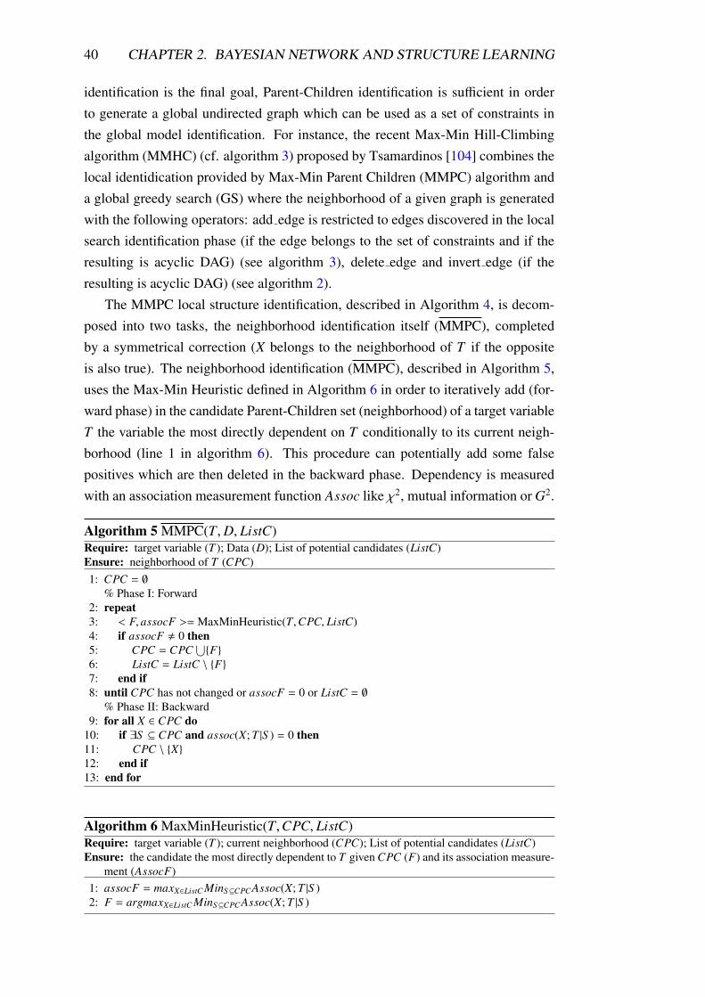
identification is the final goal, Parent-Children identification is sufficient in order
to generate a global undirected graph which can be used as a set of constraints in
the global model identification. For instance, the recent Max-Min Hill-Climbing
algorithm (MMHC) (cf. algorithm 3) proposed by Tsamardinos [104] combines the
local identidication provided by Max-Min Parent Children (MMPC) algorithm and
a global greedy search (GS) where the neighborhood of a given graph is generated
with the following operators: add edge is restricted to edges discovered in the local
search identification phase (if the edge belongs to the set of constraints and if the
resulting is acyclic DAG) (see algorithm 3), delete edge and invert edge (if the
resulting is acyclic DAG) (see algorithm 2).
The MMPC local structure identification, described in Algorithm 4, is decom-
posed into two tasks, the neighborhood identification itself (MMPC), completed
by a symmetrical correction (X belongs to the neighborhood of T if the opposite
is also true). The neighborhood identification (MMPC), described in Algorithm 5,
uses the Max-Min Heuristic defined in Algorithm 6 in order to iteratively add (for-
ward phase) in the candidate Parent-Children set (neighborhood) of a target variable
T the variable the most directly dependent on T conditionally to its current neigh-
borhood (line 1 in algorithm 6). This procedure can potentially add some false
positives which are then deleted in the backward phase. Dependency is measured
with an association measurement function Assoc like χ2, mutual information or G2.
Algorithm 5 MMPC(T,D, ListC)
Require: target variable (T ); Data (D); List of potential candidates (ListC)
Ensure: neighborhood of T (CPC)
1: CPC = ∅
% Phase I: Forward
2: repeat
3: < F, assocF >=MaxMinHeuristic(T,CPC, ListC)
4: if assocF , 0 then
5: CPC = CPC∪{F}
6: ListC = ListC \ {F}
7: end if
8: until CPC has not changed or assocF = 0 or ListC = ∅
% Phase II: Backward
9: for all X ∈ CPC do
10: if ∃S ⊆ CPC and assoc(X; T |S ) = 0 then
11: CPC \ {X}
12: end if
13: end for
Algorithm 6 MaxMinHeuristic(T,CPC, ListC)
Require: target variable (T ); current neighborhood (CPC); List of potential candidates (ListC)
Ensure: the candidate the most directly dependent to T given CPC (F) and its association measure-
ment (AssocF)
1: assocF = maxX∈ListC MinS⊆CPC Assoc(X; T |S )
2: F = argmaxX∈ListC MinS⊆CPC Assoc(X; T |S )
2.3. BAYESIAN NETWORK STRUCTURE LEARNING 41
2.3.4 Learning with large number of variables
Bayesian network learning is a useful tool for exploratory data analysis. How-
ever, applying Bayesian networks to the analysis of large-scale data, consisting of
thousands of variables, is not straight forward because of the heavy computational
burden in learning and visualization. Some studies have focused on this problem to
solve it through different approaches.
Friedman et al [33] introduce an algorithm that achieves faster learning from
massive datasets by restricting the search space. Their iterative algorithm named
”Sparse Candidate” restricts the parents of each variable to belong to a small sub-
set of candidates. They then search for a network that satisfies these constraints.
The learned network is then used to select better candidates for the next iteration.
This algorithm is based on 2 steps: the first step is named restrict based on data
D and Bn−1 network, the selected candidates for Xi’s parents include Xi’s current
parents. This requirement (restrict step) implies that the winning network Bn is
a legal structure in the n+1 iteration. Thus, if the search procedure at the sec-
ond step named maximize also examines this structure, it must return a structure
that scores at least as well as Bn. The stopping criteria for the algorithm is when
Score(Bn)=Score(Bn−1).
Steck and Jaakkola [96] look at active learning in domains with a large number
of variables. They developed an approach to unsupervised active learning which is
tailored to large domains. The computational efficiency crucially depends on the
properties of the measure with respect to which the optimal query is chosen. The
standard information gain turns out to require a committee size that scales expo-
nentially with the size of the domain (the number of random variables). Also, they
propose a new measure, which they term ”average KL divergence of pairs” (KL2).
It emerges as a natural extension to the query by the committee approach [30]. The
advantages of this approach are illustrated in the context of recovering (regulatory)
network models. The regulatory network involves 33 variables, 56 edges, and each
variable was discretized to 4 states.
In 2006, Hwangand et al [44] proposed a novel method for large-scale data
analysis based on hierarchical compression of information and constrained struc-
tural learning, i.e., hierarchical Bayesian networks (HBNs). The HBN can com-
pactly visualize global probabilistic structure through a small number of hidden
variables, approximately representing a large number of observed variables. An
efficient learning algorithm for HBNs, which incrementally maximizes the lower
bound of the likelihood function, is also suggested. They propose a two-phases
learning algorithm for hierarchical Bayesian networks based on the above decom-
position. In the first phase, a hierarchy for information compression is learned.
After building the hierarchy, they learn the edges inside a layer when necessary by
42 CHAPTER 2. BAYESIAN NETWORK AND STRUCTURE LEARNING
the second phase. The effectiveness of their method is demonstrated by the experi-
ments on synthetic large-scale Bayesian networks and a real-life microarray dataset.
All variables were binary and local probability distributions were randomly gener-
ated. In this work, they show the results on two scale-free and modular Bayesian
networks, consisting of 5000 nodes. Training datasets having 1000 examples.
Tsamardinos et al. [104] present an algorithm for the Bayesian network struc-
ture learning, called Max-Min Hill-Climbing (MMHC) described in the previous
section. They show the ability of MMHC to scale up to thousands of variables.
Tsamardinos brought the evidence of the scalability of MMHC by a reported exper-
iment in Tsamardinos et al. [102] (for example MMPC was run on each node and
reconstructed the skeleton of a tiled-ALARM network with approximately 10,000
variables from 1000 training instances).
De Campos et al [20] propose a new any-time exact algorithm using a branch-
and-bound (B&B) approach with caches. Scores are computed during the initial-
ization and a poll is built. Then, they perform the search over the possible graphs
iterating over arcs. Although iterating over orderings is probably faster, iterating
over arcs allows us to work with constraints in a straight forward way. Because of
the B&B properties, the algorithm can be stopped at any-time with a best current
solution found so far and an upper bound to the global optimum, which gives a kind
of certificate to the answer and allows the user to stop the computation when she
believes that the current solution is good enough. They show also empirically the
advantages of the properties and the constraints, and the applicability of their pre-
sented algorithm that integrates parameter and structural constraints with large data
sets (up to one hundred variables), that cannot be handled by other current meth-
ods (limited to around 30 variables), in a way to guarantee global optimality with
respect to the score function.
2.4 Evaluation of Bayesian Network structure learn-
ing algorithms
2.4.1 Evaluation metrics
In the previous sections, we presented some bayes Net structure learning algo-
rithms. In this section we present methods that evaluate the quality of the Bayesian
network obtained by the structure learning algorithms.
There are two scenarios for the evaluation of a structure learning algorithm:
– Given a theoretical BN B0 = (G0 ; θ0) and data D generated from the BN, the
measures evaluate the quality of the algorithm by comparing the quality of
the learned graph B = (G,θ) and that of the theoretical network B0 with the
2.4. EVALUATION OF BAYESIAN NETWORK STRUCTURE LEARNING ALGORITHMS43
use of data
– the measure evaluates the quality of the algorithm by comparing the structure
G of the learned graph and the structure G0 of the theoretical graph.
To this end we notice that it would be better to compare the equivalence classes
given by the original and learned BN. A BN obtained from the data is identified
by its equivalence class. The best BN is obtained if we find that the CPDAG of
the generated network is equal to that of the learned BN. So, all evaluation metrics
must use the equivalence class to compare between the BNs for better evaluation.
There are several measures proposed in the literature for the evaluation of structure
learning algorithms [76].
Score-based method
To evaluate a structure learning algorithm, many studies use a comparision be-
tween the score fuction of the learned graph and the original graph. The learning
algorithm is good if S(B,D) ⋍ S (G0,D) where S is a score among the scores given
in the previous section 2.3.2.
An advantage of this approach is that it takes into account Markov equivalence
to evaluate the structure. this metric gives the best results if there is large learned
dataset.
However, the use of score functions to evaluate the learning structure algorithms
can produce some problems. For example, if the data are limited, it is possible to
obtain a graph G with the same score as G0, but that is not in the same equivalence
class.
Kullback-Leibler divergence-based method
The Kullback-Leibler (KL) divergence is a fundamental equation of informa-
tion theory that quantifies the proximity of two probability distributions [86]. It is a
non-symmetric measure of the difference between the probability distributions of a
learned network P and the probability distributions of a target network Q. Specifi-
cally, the Kullback-Leibler divergence of Q from P, denoted DKL(P |Q), is a measure
of the information lost when Q is used to approximate P: KL measures the expected
number of extra bits required to encode samples from P when using a code based on
Q, rather than using a code based on P. Typically P represents the ”true” distribution
of data, observations, or a precisely calculated theoretical distribution. The measure
Q typically represents a theory, a model, a description, or an approximation of P.
If the variables are discrete, this divergence is defined by:
DKL(P \\ Q) =∑
x=χ
P(x) logP(x)
Q(x)(2.7)
44 CHAPTER 2. BAYESIAN NETWORK AND STRUCTURE LEARNING
DKL is non-negative (≥ 0), not symmetric in P and Q, zero if the distributions match
exactly, it can potentially equal infinity.
This metric is important when the network is used for inference. However, the
KL-divergence is not directly penalized for extraneous edges and parameters [104].
There are situations where the KL divergence has limitations. In fact, the com-
putational complexity is exponential to the number of variables. In this case, the
principle of sampling can be used to reduce this complexity.
Sensitivity and specificity-based method
Sensitivity and specificity are statistical measures of the performance of a binary
classification test, also known as classification function in statistics [29].
Sensitivity measures the proportion of actual positives which are correctly iden-
tified. Specificity measures the proportion of negatives which are correctly identi-
fied.
Given the graph of the theoretical network G0 = (V, E0) and the graph of the
learned network G = (V, E), The sensitivity-specificity-based method begins by
calculating the following indices:
– TP (true positive) = number of edges present in both G0 and G
– TN (true negative) = number of edges absent in both G0 and G
– FP (false positive) = number of edges present in G, but not in G0
– FN (false negative) = number of edges absent in G, but not in G0
Then, the sensitivity and specificity can be calculated as follows:
Sensitivity= T PT P+FN
Specificity= T NT N+FP
These measures are easy to calculate. They are often used in the literature. How-
ever, the differences in orientation between the two graphs in the same equivalence
class are counted as errors.
Distance-based method
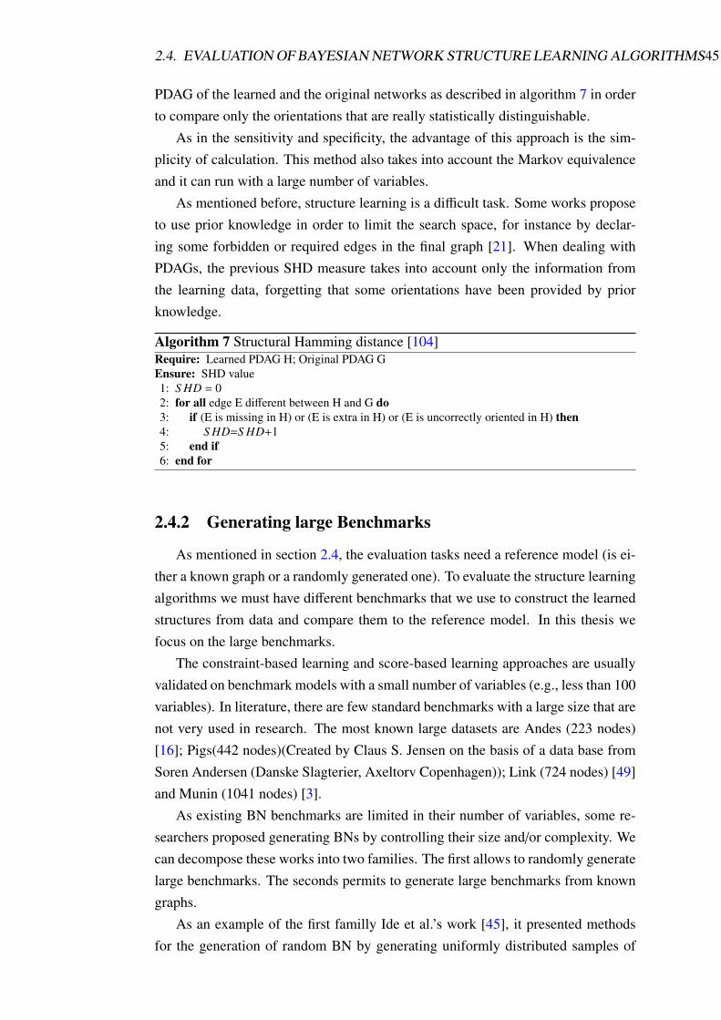
Tsamardinos et al. [104] have proposed an adaptation of the usual Hamming
distance between graphs taking into account the fact that some graphs with dif-
ferent orientations can be statistically indistinguishable. As graphical models of
independence, several equivalent graphs will represent the same set of dependence
/ independence properties. These equivalent graphs (also named Markov or likeli-
hood equivalent graphs) can be summarized by a partially DAG (PDAG) (section
2.2.4). This new structural Hamming distance (SHD) compares the structure of the
2.4. EVALUATION OF BAYESIAN NETWORK STRUCTURE LEARNING ALGORITHMS45
PDAG of the learned and the original networks as described in algorithm 7 in order
to compare only the orientations that are really statistically distinguishable.
As in the sensitivity and specificity, the advantage of this approach is the sim-
plicity of calculation. This method also takes into account the Markov equivalence
and it can run with a large number of variables.
As mentioned before, structure learning is a difficult task. Some works propose
to use prior knowledge in order to limit the search space, for instance by declar-
ing some forbidden or required edges in the final graph [21]. When dealing with
PDAGs, the previous SHD measure takes into account only the information from
the learning data, forgetting that some orientations have been provided by prior
knowledge.
Algorithm 7 Structural Hamming distance [104]
Require: Learned PDAG H; Original PDAG G
Ensure: SHD value
1: S HD = 0
2: for all edge E different between H and G do
3: if (E is missing in H) or (E is extra in H) or (E is uncorrectly oriented in H) then
4: S HD=S HD+1
5: end if
6: end for
2.4.2 Generating large Benchmarks
As mentioned in section 2.4, the evaluation tasks need a reference model (is ei-
ther a known graph or a randomly generated one). To evaluate the structure learning
algorithms we must have different benchmarks that we use to construct the learned
structures from data and compare them to the reference model. In this thesis we
focus on the large benchmarks.
The constraint-based learning and score-based learning approaches are usually
validated on benchmark models with a small number of variables (e.g., less than 100
variables). In literature, there are few standard benchmarks with a large size that are
not very used in research. The most known large datasets are Andes (223 nodes)
[16]; Pigs(442 nodes)(Created by Claus S. Jensen on the basis of a data base from
Soren Andersen (Danske Slagterier, Axeltorv Copenhagen)); Link (724 nodes) [49]
and Munin (1041 nodes) [3].
As existing BN benchmarks are limited in their number of variables, some re-
searchers proposed generating BNs by controlling their size and/or complexity. We
can decompose these works into two families. The first allows to randomly generate
large benchmarks. The seconds permits to generate large benchmarks from known
graphs.
As an example of the first familly Ide et al.’s work [45], it presented methods
for the generation of random BN by generating uniformly distributed samples of
46 CHAPTER 2. BAYESIAN NETWORK AND STRUCTURE LEARNING
directed acyclic graphs. They develop a uniform generation of multi-connected
and single-connected networks for a given number of nodes. Some studies use the
generation of random graphs. These kinds of generation have some disatvantages.
These graphs can have some repeated substructure. In addition some characteristics
can be missed.
Generating a very large BN randomly is not very realistic. In many large ap-
plications, the global model can be decomposed in coherent repeated subgraphs. In
the second familly, they chose the reference model as multi-copies of the original
standard model. Tsamardinos et al, in [95], have proposed a novel algorithm and
software for the generation of an arbitrary large BN (e.g., graphical models rep-
resentation and joint probability distributions) by tiling smaller real-world known
networks (tiles). The complexity of the final model is controlled by two param-
eters : the number of tiling n and the connectivity parameter c which determines
the maximum number of connections between one node and the next tile. In litera-
ture, to solve the problems given by generation of random BN, most of the studies
[104, 22, 39] use tiling to generate large benchmarks and use them for the valida-
tion of their learning algorithms. In these works, they use tiling of small standard
Benchmarks as (Asia, Alarm and Hailfinder) by tiling the original structure 3, 5 and
10 times.
As far as we know, the tiling technique is the best and most useful algorithm for
simulating large BNs. In fact, during our research, we have found that the Tiling
was used in many studies, such as to compare different Markov Blanket learning
algorithms in large (5000 variables) networks [105, 102]; or to compare many BN
learning algorithms in [104, 6, 56, 39], and to examine the time efficiency and qual-
ity of a local BN learning algorithm to reconstruct local regions in a large (10000
variable) network in [104].
2.5 Conclusion
In this chapter, we proceeded by presenting the concepts of Bayesian networks,
then we reviewed the different structure learning methods of these models. We also
addressed the question of evaluation for these learning algorithms.
We have seen that the hybrid method for learning the BN perform better than
others techniques based on constraints or on score on the level of scalability and
complexity of algorithms.
Section 2.4 presented an overview of the evaluation methods. The score-based
method takes into account the equivalence of Markov during the evaluation. But
if the data were reduced, it would be difficult to distinguish two different networks
by their scores. Other methods based on reference model are also able to take into

2.5. CONCLUSION 47
account Markov equivalence, though the calculation is costly when the number of
variables is important.
In the next chapter we will introduce an extension of the Bayesian networks
named Dynamic Bayesian Network. This kind of model is a special Bayesian Net-
work, which is used with dynamic stochastic process models [73].

3Dynamic Bayesian Networks and
structure learning
Sommaire
3.1 Introduction . . . . . . . . . . . . . . . . . . . . . . . . . . . 50
3.2 Dynamic Bayesian Network Definition . . . . . . . . . . . . . 50
3.2.1 Representation . . . . . . . . . . . . . . . . . . . . . . 50
3.2.2 Different forms of K-TBN . . . . . . . . . . . . . . . . 51
2-TBN . . . . . . . . . . . . . . . . . . . . . . . . . . 51
k-TBN . . . . . . . . . . . . . . . . . . . . . . . . . . 52
Simplified k-TBN . . . . . . . . . . . . . . . . . . . . 53
Other DBN forms . . . . . . . . . . . . . . . . . . . . . 54
3.3 Dynamic Bayesian Network structure learning . . . . . . . . 55
3.3.1 Principle . . . . . . . . . . . . . . . . . . . . . . . . . 55
3.3.2 Structure learning approaches for 2-TBN and k-TBN mod-
els . . . . . . . . . . . . . . . . . . . . . . . . . . . . . 55
3.3.3 Structure learning approaches for simplified ”k-TBN and
2-TBN” models . . . . . . . . . . . . . . . . . . . . . . 56
3.3.4 Structure learning approaches for other forms of DBN
models . . . . . . . . . . . . . . . . . . . . . . . . . . 57
3.4 Evaluation of DBN structure learning algorithms . . . . . . . 58
3.4.1 Benchmarks . . . . . . . . . . . . . . . . . . . . . . . . 58
3.4.2 Evaluation metric . . . . . . . . . . . . . . . . . . . . . 59
3.5 Conclusion . . . . . . . . . . . . . . . . . . . . . . . . . . . . 60
49
50CHAPTER 3. DYNAMIC BAYESIAN NETWORKS AND STRUCTURE LEARNING
3.1 Introduction
It is natural to use a dynamic Bayesian network (DBN), a directed graphical
model whose nodes are across different time slices, to learn and reason about dy-
namic systems. DBN model is a temporal process and use a conditional probability
distribution for each node and a probabilistic transition between time slices.
It is generally assumed that a DBN model structure and parameters do not
change over time, i.e., the model is time-invariant [73]. Learning a DBN model
from data aims to find the best model of the unknown probability distribution un-
derlying the temporal process on the basis of a random sample of a finite size, i.e.
the learning data.
As the static case, the learning dynamic Bayesian network consists of two phases:
learning of the parameters and the learning of the structure. In the dynamic context
most of the structure learning methods for DBN are based on the optimization of a
score and deal with small dimension of benchmarks. Some recent works use hybrid
methods (local search identification and global optimisation). However, this kind of
methods deals with large dimension of benchmarks on a ”simplified” search space.
As mentioned in Chapter 2, all studies try to evaluate their structure learning
algorithms through some evaluation techniques. Many studies tried to know the
goodness of their methods with the help of a scoring criterion, which is not the best
way as we presented in section 2.4.1.
This chapter deals with basic definitions and notations of dynamic (temporal)
Bayesian networks. Section 2.2 introduces some DBN notations and definitions.
Section 2.3 provides an overview of the dynamic Bayesian networks structure learn-
ing. And as in the previous chapter, section 2.4 presents some techniques for the
evaluation of Bayesian networks structure. Also, in this section we present what the
existing approaches used to evaluate these structure learning algorithms on small
and large Benchmarks. Finally, we try to enumerate the different limitations of the
structure learning and evalution.
3.2 Dynamic Bayesian Network Definition
3.2.1 Representation
A dynamic Bayesian network (DBN) is a probabilistic graphical model devoted
to represent sequential systems. More precisely, a DBN defines the probability
distribution of a collection of random variables X[t] where X = {X1 . . . Xn} is the set
of variables observed along discrete time t [23, 73].
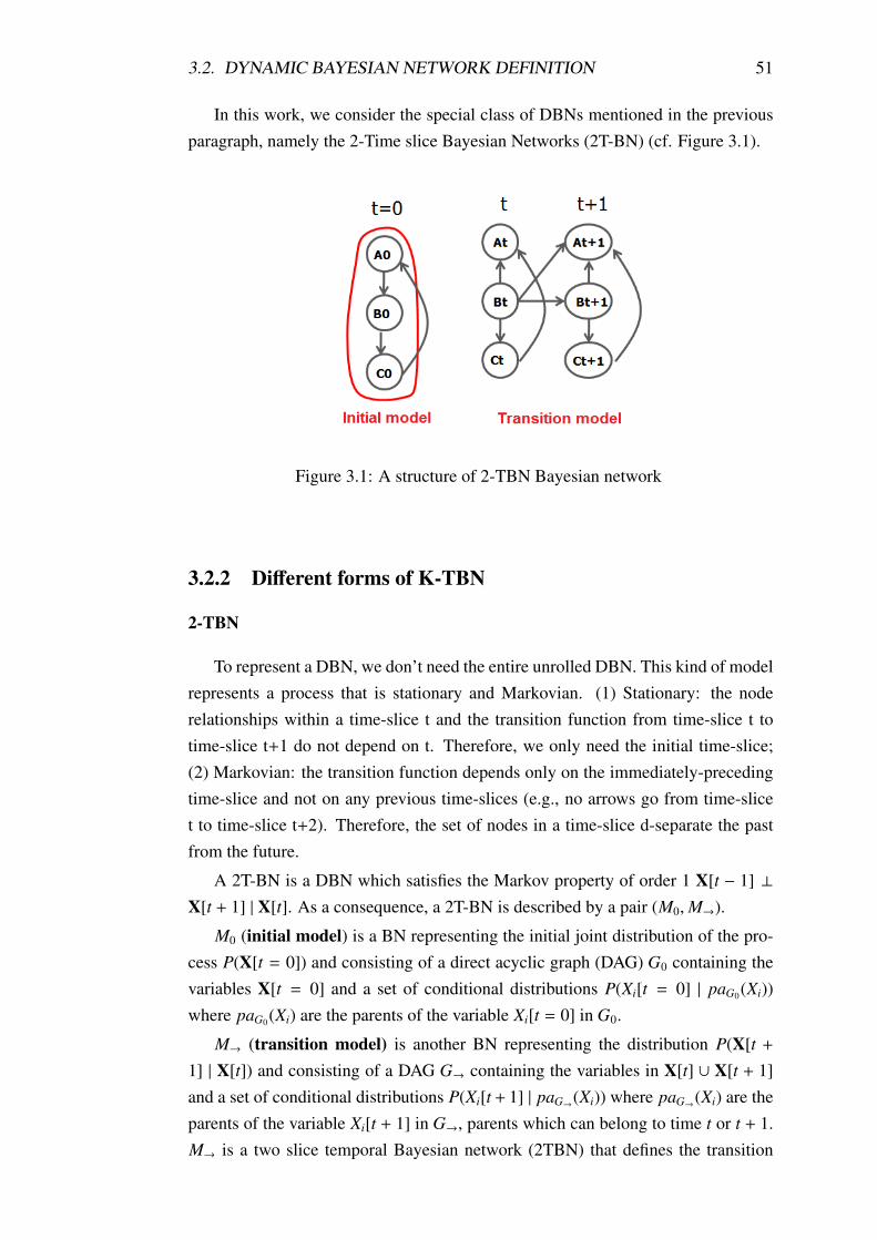
3.2. DYNAMIC BAYESIAN NETWORK DEFINITION 51
In this work, we consider the special class of DBNs mentioned in the previous
paragraph, namely the 2-Time slice Bayesian Networks (2T-BN) (cf. Figure 3.1).
Figure 3.1: A structure of 2-TBN Bayesian network
3.2.2 Different forms of K-TBN
2-TBN
To represent a DBN, we don’t need the entire unrolled DBN. This kind of model
represents a process that is stationary and Markovian. (1) Stationary: the node
relationships within a time-slice t and the transition function from time-slice t to
time-slice t+1 do not depend on t. Therefore, we only need the initial time-slice;
(2) Markovian: the transition function depends only on the immediately-preceding
time-slice and not on any previous time-slices (e.g., no arrows go from time-slice
t to time-slice t+2). Therefore, the set of nodes in a time-slice d-separate the past
from the future.
A 2T-BN is a DBN which satisfies the Markov property of order 1 X[t − 1] ⊥
X[t + 1] | X[t]. As a consequence, a 2T-BN is described by a pair (M0,M→).
M0 (initial model) is a BN representing the initial joint distribution of the pro-
cess P(X[t = 0]) and consisting of a direct acyclic graph (DAG) G0 containing the
variables X[t = 0] and a set of conditional distributions P(Xi[t = 0] | paG0(Xi))
where paG0(Xi) are the parents of the variable Xi[t = 0] in G0.
M→ (transition model) is another BN representing the distribution P(X[t +
1] | X[t]) and consisting of a DAG G→ containing the variables in X[t] ∪ X[t + 1]
and a set of conditional distributions P(Xi[t + 1] | paG→(Xi)) where paG→(Xi) are the
parents of the variable Xi[t + 1] in G→, parents which can belong to time t or t + 1.
M→ is a two slice temporal Bayesian network (2TBN) that defines the transition
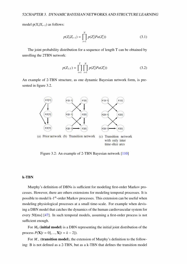
52CHAPTER 3. DYNAMIC BAYESIAN NETWORKS AND STRUCTURE LEARNING
model p(Xt|Xt−1) as follows:
p(Zt|Zt−1) =
N∏
t=1
p(Zit |Pa(Zi
t)) (3.1)
The joint probability distribution for a sequence of length T can be obtained by
unrolling the 2TBN network:
p(Z1:T ) =
T∏
t=1
N∏
i=1
p(Zit |Pa(Zi
t)) (3.2)
An example of 2-TBN structure, as one dynamic Bayesian network form, is pre-
sented in figure 3.2.
Figure 3.2: An example of 2-TBN Bayesian network [110]
k-TBN
Murphy’s definition of DBNs is sufficient for modeling first-order Markov pro-
cesses. However, there are others extensions for modeling temporal processes. It is
possible to model k-1th-order Markov processes. This extension can be useful when
modeling physiological processes at a small time-scale. For example when devis-
ing a DBN model that catches the dynamics of the human cardiovascular system for
every 50[ms] [47]. In such temporal models, assuming a first-order process is not
sufficient enough.
For M0 (initial model) is a DBN representing the initial joint distribution of the
process P(X[t = 0], ...,X[t = k − 2]).
For M� (transition model), the extension of Murphy’s definition to the follow-
ing: B is not defined as a 2-TBN, but as a k-TBN that defines the transition model
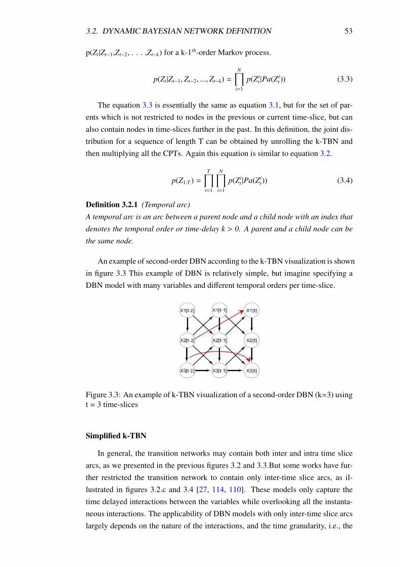
3.2. DYNAMIC BAYESIAN NETWORK DEFINITION 53
p(Zt|Zt−1,Zt−2, . . . ,Zt−k) for a k-1th-order Markov process.
p(Zt|Zt−1,Zt−2, ..., Zt−k) =
N∏
i=1
p(Zit |Pa(Zi
t)) (3.3)
The equation 3.3 is essentially the same as equation 3.1, but for the set of par-
ents which is not restricted to nodes in the previous or current time-slice, but can
also contain nodes in time-slices further in the past. In this definition, the joint dis-
tribution for a sequence of length T can be obtained by unrolling the k-TBN and
then multiplying all the CPTs. Again this equation is similar to equation 3.2.
p(Z1:T ) =
T∏
t=1
N∏
i=1
p(Zit |Pa(Zi
t)) (3.4)
Definition 3.2.1 (Temporal arc)
A temporal arc is an arc between a parent node and a child node with an index that
denotes the temporal order or time-delay k > 0. A parent and a child node can be
the same node.
An example of second-order DBN according to the k-TBN visualization is shown
in figure 3.3 This example of DBN is relatively simple, but imagine specifying a
DBN model with many variables and different temporal orders per time-slice.
Figure 3.3: An example of k-TBN visualization of a second-order DBN (k=3) using
t = 3 time-slices
Simplified k-TBN
In general, the transition networks may contain both inter and intra time slice
arcs, as we presented in the previous figures 3.2 and 3.3.But some works have fur-
ther restricted the transition network to contain only inter-time slice arcs, as il-
lustrated in figures 3.2.c and 3.4 [27, 114, 110]. These models only capture the
time delayed interactions between the variables while overlooking all the instanta-
neous interactions. The applicability of DBN models with only inter-time slice arcs
largely depends on the nature of the interactions, and the time granularity, i.e., the
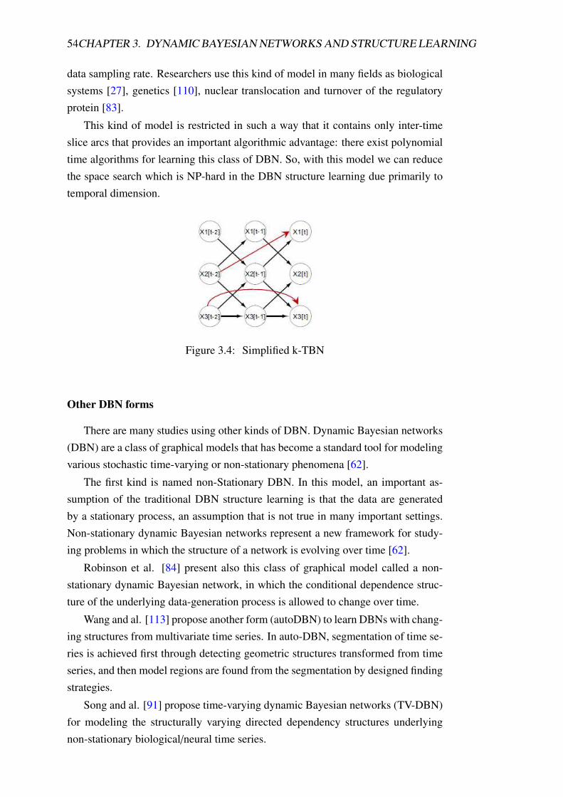
54CHAPTER 3. DYNAMIC BAYESIAN NETWORKS AND STRUCTURE LEARNING
data sampling rate. Researchers use this kind of model in many fields as biological
systems [27], genetics [110], nuclear translocation and turnover of the regulatory
protein [83].
This kind of model is restricted in such a way that it contains only inter-time
slice arcs that provides an important algorithmic advantage: there exist polynomial
time algorithms for learning this class of DBN. So, with this model we can reduce
the space search which is NP-hard in the DBN structure learning due primarily to
temporal dimension.
Figure 3.4: Simplified k-TBN
Other DBN forms
There are many studies using other kinds of DBN. Dynamic Bayesian networks
(DBN) are a class of graphical models that has become a standard tool for modeling
various stochastic time-varying or non-stationary phenomena [62].
The first kind is named non-Stationary DBN. In this model, an important as-
sumption of the traditional DBN structure learning is that the data are generated
by a stationary process, an assumption that is not true in many important settings.
Non-stationary dynamic Bayesian networks represent a new framework for study-
ing problems in which the structure of a network is evolving over time [62].
Robinson et al. [84] present also this class of graphical model called a non-
stationary dynamic Bayesian network, in which the conditional dependence struc-
ture of the underlying data-generation process is allowed to change over time.
Wang and al. [113] propose another form (autoDBN) to learn DBNs with chang-
ing structures from multivariate time series. In auto-DBN, segmentation of time se-
ries is achieved first through detecting geometric structures transformed from time
series, and then model regions are found from the segmentation by designed finding
strategies.
Song and al. [91] propose time-varying dynamic Bayesian networks (TV-DBN)
for modeling the structurally varying directed dependency structures underlying
non-stationary biological/neural time series.
3.3. DYNAMIC BAYESIAN NETWORK STRUCTURE LEARNING 55
3.3 Dynamic Bayesian Network structure learning
The existing techniques for learning DBNs are mostly straightforward exten-
sions of the techniques for learning BNs [73]. In this thesis, we only focus on the
structure learning in DBN. Before explaining the structure learning in a DBN, We
mentioned that to achieve parameter learning, we can use the techniques discussed
in Appendix A. In this case, we just comment on two points that are applicable
specifically to dynamic systems: (1) Parameters must be tied across time-slices, so
we can model sequences of unbounded length; (2) The parameters, π, for P(X1) are
usually taken to represent the initial state of the dynamic system [73].
3.3.1 Principle
As in Murphy’s definition, the structure learning of a DBN has some assump-
tions must be respected:
– Learning the intra-slice connectivity, which must be a DAG,
– Learning the inter-slice connectivity, which is equivalent to the variable se-
lection problem, since for each node in slice t, we must choose its parents
from slice t-1.
– If we assume the intra-slice connections to be fixed, this means that structure
learning for DBNs reduces to feature selection (simplified search space). If
the system is fully observed (complete data), we can apply standard feature
selection algorithms, such as forward or backwards stepwise selection, or the
leaps and bounds algorithm [73].
When the system is partially observed (incomplete data), the structure learning
becomes computationally intensive. One practical approach is the structural EM
(SEM) algorithm [31].
3.3.2 Structure learning approaches for 2-TBN and k-TBN mod-
els
Friedman et al. [32] have shown that this task can be decomposed in two inde-
pendent phases: learning the initial graph G0 as a static BN structure with a static
dataset corresponding to X[t = 0] and learning the transition graph M→ with an-
other ”static” dataset corresponding to all the transitions X[t] ∪X[t + 1]. They then
proposed to apply usual score-based algorithms such as greedy search (GS) in order
to find both graphs. Learning dynamic Bayesian network structures provides a main
mechanism for identifying conditional dependencies in time-series data.
[35] developed another evolutionary approach for 2T-BN structure learning. In
this work, The DBN structure learning based on BOA consists of two parts. The
first part is to obtain the structure and parameters of the DBN in terms of a good
56CHAPTER 3. DYNAMIC BAYESIAN NETWORKS AND STRUCTURE LEARNING
solution, and the second part is to produce new groups according to the obtained
DBN structure. Wang and al. [112] also look at using evolutionary computation in
2T-BN structure learning by incorporating sampling methods.
Some other research work in structure learning propose their own algorithm for
learning in such domains as the medicine, biology, geometry. Rajapakse et al. [82]
use the dynamic Bayesian networks (DBN) and a Markov chain to model fMRI
time-series and thereby determine temporal relationships of interactions among
brain regions. Experiments on synthetic fMRI data demonstrate that the perfor-
mance of the DBN is comparable to Granger causality mapping (GCM) in deter-
mining the structure of linearly connected networks.
Pena et al. [81] study cross-validation as a scoring criterion for learning dy-
namic Bayesian network models that can be well generalized. they argue that cross-
validation is more suitable than the Bayesian scoring criterion as one of the most
common interpretations of generalization.
Aydin and al. [5] present a secondary structure prediction method that employs
dynamic Bayesian networks and support vector machines. This work is applied on
biology.
All these approaches are validated on small benchmark models (with about 10
variables). In a more general context, due to inherent limitations of score-based
structure learning methods, all these methods will have a very high complexity if
the number of variables increases.
3.3.3 Structure learning approaches for simplified ”k-TBN and
2-TBN” models
Dojer [27] offers an algorithm for learning an optimal network structure. It
works in polynomial time for both MDL and BDe scores. His method is addressed
to the case when the benchmark is small and there is no need to examine the acyclic-
ity of the graph. According to Dojer, the second assumption is satisfied in the DBN
case. In fact, as he mentioned in his work, A DBN describes a stochastic evolution
of a set of random variables over discretized time. Therefore conditional distribu-
tions refer to random variables in neighboring time points. The acyclicity constraint
is relaxed, because the”unrolled” graph is always acyclic.
In 2009, Wilczynski et al. [114] implemented and ran the previous Dojer’s al-
gorithm. He presented in a BNFinder software, which allows the Bayesian network
reconstruction from experimental data. It supports dynamic Bayesian networks.
Vinh et al. dealt particularly with the problem of learning the globally optimal
structure of a dynamic Bayesian network (DBN) [111]. They said that the MIT
(Mutual Information Test) is better for evaluating the goodness-of-fit of the DBN
structure than the other popular scoring metrics, such as BIC/MDL, K2 and BD,
3.3. DYNAMIC BAYESIAN NETWORK STRUCTURE LEARNING 57
and the well-known constraint-based PC algorithm.
Vinh et al. [110] propose another score based algorithm without equicardinality
assumptions named MIT-global. Also, they propose another contribution in this
work consist of a hybrid method with local Blanket identification (MIT-MMMB).
They show that the local search MIT-MMMB and global-MIT have similar results
better than advanced score based algorithm (simulated annealing). The MIT based
on MMMB try to identify the Markov Blanket MB but in a restricted subclass of
2T-BNs named simplified 2-TBN (cf. figure 3.2.c) or kT-BNs (cf. figure 3.3). This
assumption permits to simplify both the MB discovery and the global optimization
but it is not able to identify the intra-time dependencies.
3.3.4 Structure learning approaches for other forms of DBN mod-
els
Tucker et al. have developed an evolutionary algorithm which exploits certain
characteristics of the MTS process in order to generate good networks as quickly
as possible. They compare this algorithm to other standard learning algorithms that
have traditionally been used for static Bayesian networks but adapted for DBNs
[108].
The work of Wyncoop and al.[115] addresses the problem of learning dynamic
Bayesian network (DBN) models to support the reinforcement of learning. It fo-
cuses on the learning regression tree (context-specific dependence) models of the
conditional probability distributions of the DBNs. In this study, they introduce a
regression tree algorithm in which each leaf node is modeled as a finite mixture of
deterministic functions. This mixture is approximated via a greedy set cover.
In the work of Wang et al. [113], the auto-DBN model permits a segmentation of
time series achieved first through detecting geometric structures transformed from
time series, and then the model regions are found from the segmentation by de-
signed finding strategies; in each found model region, a DBN model is established
by existing structure learning methods; Finally, a model revisiting is developed to
refine model regions and improve DBN models. These techniques provide a special
mechanism to find accurate model regions and discover a sequence of DBNs with
changing structures, which are adaptive to changing relations between multivariate
time series.
Robinson et al. [84] define the non-stationary DBN model, present an MCMC
sampling algorithm to efficiently learn the structure of an nsDBN and the times of
non-stationarities (transition times) under different assumptions, and demonstrate
the effectiveness of the algorithm on simulated data.
58CHAPTER 3. DYNAMIC BAYESIAN NETWORKS AND STRUCTURE LEARNING
3.4 Evaluation of DBN structure learning algorithms
All works for structure learning in literature develop an experimental study to
present the goodness of their DBN structure learning algorithms . There are popular
tools for the evaluation of the learning from time-series data. In this section we
present the existing methods to evaluate structure learning algorithms for the DBN.
3.4.1 Benchmarks
The first step to evaluate the performance of these algorithms is to assemble
different standard benchmarks. In Pena’s work [81], the authors involve learning
databases of different sizes sampled from a partial model of the transcriptional reg-
ulatory network of Saccharomyces cerevisiae. The model involves 30 transcription
or (variables) factors and 56 interactions (dependences) between them.
In [50], the authors ran experiments with their DBN learning approach in the
coffee task [9] (containing 6 variables), Taxi task [25] (containing 10 variables), and
a simplified autonomous guided vehicle (AGV) task [38] (containing 20 variables).
Gao et al. [35] select DBNs that have 8 variables to match the database as an
optimization object. They use the database from BNT Structure Learning Package
[61].
Rajapakse et al. [82] illustrate their method with experiments on synthetic data
as well as on two real fMRI datasets from fMRI Data Center, Dartmouth College
(fMRIDC, 2004) (containing 5 variables).
Wang et al. [113] use a real data set, it is about the interest rates of Australia,
France, UK and US in 240 months from July 1980 to June 2000 [65] with three vari-
ables. Another real data set is about daily stock prices of ten aerospace companies
from January 1988 to October 1991 [1] with six variables.
Song [91] conducted 3 experiments using synthetic data, gene expression data
and EEG signals. they generate 8 different anchor transition matrices A1t : : :
A8t , each of which corresponds to a random graph of node size n=50 and average
in degree of 2 (they have also experimented with n = 75 and 100 which provides
similar results).
Finally in Hwang’s work [43], the writers gathered video data recorded at sev-
eral intersections and used them to detect accidents at different intersections which
have different traffic flows and intersection designs. A total of 70 video scripts are
used in the experiments, containing 33 accidents, 10 situations similar to accidents,
and 27 normal situations. The model studied in this work contains 10 variables.
Although all the works interested in DBN structure learning generally use small
benchmarks size, there are some other recent works as try to improve this disad-
vantage of the DBN structure learning. They use large benchmarks to run their
3.4. EVALUATION OF DBN STRUCTURE LEARNING ALGORITHMS 59
algorithms.
Dojer [27] tested the time complexity of learning an optimal dynamic BN on
microarray experiments data of Arabidopsis thaliana (≈23 000 genes). The running
time computed was about 48 hours for the MDL score and 170 hours for the BDe
score.
In order to judge the performance of their software, [114] have compared it to
the Banjo library. As a realistic dataset, we have chosen the dataset attached as an
example to the Banjo package, consisting of 20 variables and 2000 observations,
published by Smith et al. [90].
Vinh et al [111] employ several synthetic data sets generated by different data
generation schemes that have been used in some previous studies. As a realistic
number of samples for microarray data, they generated data sets of between 30 and
300 samples. With the ground-truth network available, they count the number of
true positive (TP), false positive (FP), true negative (TN) and false negative (FN)
edges, and report two network quality metrics, namely sensitivity and specificity.
In 2012, Vin et al. [110] proposed a study where the experimental study has
been conducted with about 1595 variables.
3.4.2 Evaluation metric
We remark in this study that, like the static BNs, the structure learning for DBNs
studies use the score functions or comparison between graphs to evaluate the per-
formance of algorithms. Contrary to the static BN, that has many metrics used for
evaluation as we mentioned in section 2.4. Also, in DBNs studies, we didn’t find
standard metrics that can be used as the SHD in tthestatic case.
[50] compared their active learning scheme with passive learning . In this case,
they use the BIC and BDe scores to detect most of the refinements necessary to
learn the true DBN model.
[35] used fitness function for a DBN, there exist two structure measure scales,
namely, Bayesian Dirichlet metric (BD) and Bayesian information metric (BIC). In
their paper, they use BD to measure network.
[82] used the square error e2 between the true connectivity structure C= {ci j} and
the estimated structure = {¢i j} is measured by the square error between the elements
of the matrices defining the structures:
e2 =1
2n2
n∑
i=1
n∑
j=1
(ci j − ¢i j)2 (3.5)
the elements c and ¢ were scaled to the range [0,1] for comparison purposes
with other approaches
Song et al evaluate the performance using an F1 score, which is the harmonic
60CHAPTER 3. DYNAMIC BAYESIAN NETWORKS AND STRUCTURE LEARNING
mean of sensitivity and scores call-function in retrieving the true time-varying net-
work edges [91].
In [43] they used the fitness function as a metric to evaluate the performance of
population for the given problem. Fitness function, therefore, evaluates the suitabil-
ity of a dynamic Bayesian network structure.
As we mentioned above most of theworks use score functions for the evalua-
tion step. However, there are a few works that use large datasets to evaluate their
approaches. They use some other techniques of evaluation. Dojer and Wilczynski
[27, 114] use computation running time as measure. Vinh et al. in [111] use three
features: the percent sensitivity, the percent imprecision and the running time. Vinh
et al. in [110] use node degree or connectivity degree distribution and runtime to
compare the performance of their algorithms to others algorithms.
We remark that all these studies used the running time as a common metric for
the evaluation. This is explained by the fact that in high dimension it is not enough
to show the reliability of system but the time is an important factor for the evaluation
process.
3.5 Conclusion
In this chapter, after presenting the key concepts of Dynamic Bayesian network,
we reviewed the different structure learning studies of these models in literature.
We also addressed the topic of how the different works proceded to evaluate their
learning algorithms.
In section 2.4, we focused on presenting an overview of the evaluation methods.
The important conclusion reached in this study, is that the structure learning in the
dynamic Bayesian Network has many disatvantages. This conclusion was given by
many points:
Firstly, most of the works use networks with a small number of variables. This
choice is explained by the fact that all works for learning structure are based on
score and we showed previously that these methods of learning can’t achieve a
good performance when we increase the number of variables. we noted in previous
section that the score function takes into account the equivalence of Markov in the
evaluation. If an algorithm returns a graph G equivalent to G0, both structures have
the same score. This advantage is also a disadvantage, since if there is little data, it
is possible to obtain a graph G with the same score G0, but that is not in the same
equivalence class. We think that this choice was taken by all these studies because
of all the limitations mentioned before.
Secondly, all the studies about the DBN structure learning use their own bench-
marks and techniques for evaluation. The problem in the dynamic case is that we

3.5. CONCLUSION 61
don’t find previous works that provide details about the used networks and indica-
tors of comparison. In addition, the access to the datasets and the source code is not
always possible.
The last point, concerns the way of dealing with high dimension. The existing
works, such as Vinh et al. [110], consider a restricted subclass of 2T-BN (eg. they
learn only the inter-slice connectivity and ignore the intra-slice connectivity).
In the remaining chapters we will describe our contributions at the level of learn-
ing the DBN structure using the hybrid methods and we developed some techniques
to evaluate these learning algorithms. These techniques are standard, and can be
used with any other technique and on any standard large Benchmark. Also, they
allow the amelioration of the evaluation quality with the insertion of a priori knowl-
edge.


II
Contributions
63

4Benchmarking dynamic Bayesian
networks
Sommaire
4.1 Introduction . . . . . . . . . . . . . . . . . . . . . . . . . . . 66
4.2 Generation of large k-TBN and simplified k-TBN . . . . . . 67
4.2.1 Principle . . . . . . . . . . . . . . . . . . . . . . . . . 67
4.2.2 Tiling the initial model . . . . . . . . . . . . . . . . . . 67
4.2.3 Tiling the transition model . . . . . . . . . . . . . . . . 68
4.3 Evaluation of k-TBN generated by data and prior knowledge 69
4.3.1 Principle . . . . . . . . . . . . . . . . . . . . . . . . . 69
PDAG with knowledge . . . . . . . . . . . . . . . . . . 70
SHD(2T-BN) advantages . . . . . . . . . . . . . . . . . 71
4.4 Validation examples . . . . . . . . . . . . . . . . . . . . . . . 72
4.4.1 2-TBN Benchmark generation . . . . . . . . . . . . . . 72
Implementation . . . . . . . . . . . . . . . . . . . . . . 72
Toy example . . . . . . . . . . . . . . . . . . . . . . . 72
4.4.2 SHD for 2-TBN . . . . . . . . . . . . . . . . . . . . . . 74
Implementation . . . . . . . . . . . . . . . . . . . . . . 74
Toy example . . . . . . . . . . . . . . . . . . . . . . . 74
4.5 Conclusion . . . . . . . . . . . . . . . . . . . . . . . . . . . . 75
65
66 CHAPTER 4. BENCHMARKING DYNAMIC BAYESIAN NETWORKS
4.1 Introduction
During the last two decades, there has been an increasing interest in the Bayesian
Network (BN) formalism [78, 42]. The BNs have been recognized as one of the
most successful complete and consistent formalisms for the acquisition and repre-
sentation of knowledge and for reasoning from incomplete and/or uncertain data.
This success is due to the following factors: (1) their mathematical bases are rigor-
ously justified; (2) they deal in an innate way with uncertainty (modeled as a joint
probability distribution); (3) they are understandable (graphical representation); and
(4) they take advantage of locality both in knowledge representation and during in-
ference.
Learning the graphical part (i.e. the structure) of these models from data is an
NP-hard problem. Many studies have been conducted on this subject [12, 11, 13].
Most of these works and their result interpretations use standard networks and com-
mon performance indicators, such as the approximation of the marginal likelihood
of the obtained model or comparison of the resulting graph to the original graph
given in benchmarking tasks with the help of the Structural Hamming Distance
(SHD) proposed by Tsamardinos [104].
Dynamic Bayesian networks (DBNs) are a general and flexible model class
for the represention of complex stochastic temporal processes [73]. Some struc-
ture learning algorithms have been proposed, adapting principles already used in
”static” BNs. Comparing these algorithms is a difficult task because the evaluation
techniques and/or the reference networks used differ across research works. The
evaluation of these algorithms is also often restricted to networks with a small num-
ber of variables. However, with the static BNs, the evaluation was carried out using
a large number of variables.
In this chapter, we highlight our two major contributions: section 4.2 presents an
algorithm for generating large 2-TBN networks (which could be used as standard 2-
TBN benchmarks) using the tiling approach (see section 2.4.2) in the dynamic case;
section 4.3 presents an algorithm for the evaluation of a 2-TBN structure learning
algorithm adapting the SHD measure (section 2.4.1) no more correct with temporal
networks. Finally, we show in section 4.4 some validation examples to prove the
advantages of our methods. Our work can be a useful tool for benchmarking any
2-TBN structure learning algorithm in a common framework.

4.2. GENERATION OF LARGE K-TBN AND SIMPLIFIED K-TBN 67
4.2 Generation of large k-TBN and simplified k-TBN
4.2.1 Principle
In order to generate a large k-TBN or a simplified model, we propose generating
two models M0 and M� from an initial static benchmark BN M.
First we use the Tsamardinos’ work for the generation of realistic large bayesian
networks by tiling (section 2.4.2). We have used tiling approach because in the case
of k-TBN (M0 and M�) can be seen as a model obtained by one first tiling to gen-
erate M0 from M and another one to generate M� from M0 when it is assumed that
all the ”intra slices” dependencies (dependencies between the variables in the same
time slice) can be found at any time and the ”inter slices” dependencies (depen-
dencies between the variables in the successive time slices) can be repeated all the
time.
In the case simplified k-TBN, we start with an empty model M. The tiling algo-
rithm prevents the construction of ”intra slices” dependencies and allows the ”inter
slices” dependencies. Our method consists in generating a large initial model M0
and its conditional probability distribution by tiling n copies of the initial model M.
Then we use tiling again to generate M� and the transition probability distribution
by tiling k copies of M0.
Our suggestion is described in Algorithm 8. The complexity of the final k-TBN
can be controlled by changing the number of tiling copies and the intra-connectivity
ci (used to generate M0) or the temporal connectivity ct (used to generate temporal
edges).
Algorithm 8 Generation of large k-TBNs (TileBN for kT-BN)
Require: BN M, number of copies n, intra-connectivity ci, temporal connectivity ct
Ensure: Return initial M0 and transition models M�
1: M0 = bn tiling(M,n,ci)
2: M� = bn tiling(M0,k,ct)
4.2.2 Tiling the initial model
In this first step of generation, the algorithm needs to enter a Bayesian network BN
M with a number n of tiles desired as an input and BN1;: : : ;BNn and an integer-
valued connectivity parameter ci controlling the number of introduced edges as an
output of the algorithm. The algorithm returns the initial model characterized by a
large Bayesian network consisting of tiles with the new edges between tiles. The
joint probability distribution of the tiles is preserved. Also, our algorithm adds the
number of level used for tiling as an optional parameter (cf. figure 4.1) (i.e. we give
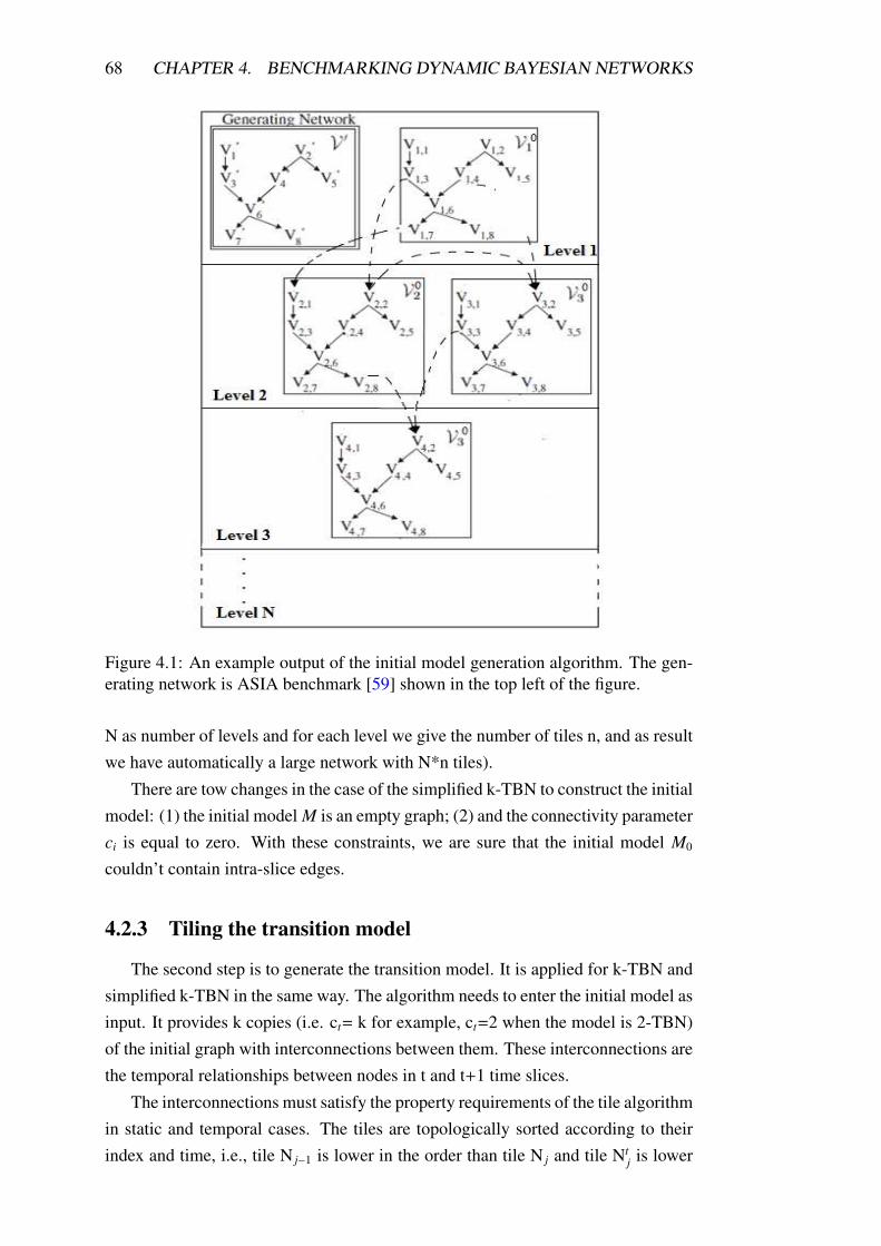
68 CHAPTER 4. BENCHMARKING DYNAMIC BAYESIAN NETWORKS
Figure 4.1: An example output of the initial model generation algorithm. The gen-
erating network is ASIA benchmark [59] shown in the top left of the figure.
N as number of levels and for each level we give the number of tiles n, and as result
we have automatically a large network with N*n tiles).
There are tow changes in the case of the simplified k-TBN to construct the initial
model: (1) the initial model M is an empty graph; (2) and the connectivity parameter
ci is equal to zero. With these constraints, we are sure that the initial model M0
couldn’t contain intra-slice edges.
4.2.3 Tiling the transition model
The second step is to generate the transition model. It is applied for k-TBN and
simplified k-TBN in the same way. The algorithm needs to enter the initial model as
input. It provides k copies (i.e. ct= k for example, ct=2 when the model is 2-TBN)
of the initial graph with interconnections between them. These interconnections are
the temporal relationships between nodes in t and t+1 time slices.
The interconnections must satisfy the property requirements of the tile algorithm
in static and temporal cases. The tiles are topologically sorted according to their
index and time, i.e., tile N j−1 is lower in the order than tile N j and tile Ntj
is lower
4.3. EVALUATION OF K-TBN GENERATED BY DATA AND PRIOR KNOWLEDGE69
in the order than tile Nt+1j
. Just as in the static case, TileBN for 2-TBN uses the
number of the randomly selected interconnecting edges between the network in t-1
time slice and network in t time slice. TileBN for 2-TBN may add the edge Vt−1p,k
�
Vtq, j
if the following four requirements are satisfied:
1. p , q, i.e., the edge goes from a variable to another belonging to a tile down-
stream (not allowed any cycle) [106]. This requirement is always checked
because Vp,k is in time slice t-1 and Vq, j is in time slice t.
2. Pa j = �;, i.e., the node V′
j of the generating network that corresponds to the
endpoint of the edge Vt−1, j is a minimal node in the generating network (it has
no parents) [106].
3. If there exists another edge Vt
p′,k′�Vt
q, j′ to the same tile q then j = j
′
, i.e.,
for each tile q only one minimal node can receive tile interconnecting edges.
The second and third requirements will be used to determine the probabilistic
properties of the output network [106].
4. All the interconnections go from a variable in t-1 to a variable in t (not allowed
to invert any temporal edges).
We notice that the first three requirements are satisfied in the static case, i.e., we
use these proprieties to construct the initial model. However, the last requirement is
used when the algorithm links between BNt and BNt+1.
The DBN definition is unrolled for k + 1 time-slices where k denotes the tem-
poral order of the Markov process. The DBN needs to be unrolled for this number
of time-slices, because in the resulting unrolled network every CPD that needs to be
learned will be represented with at least one copy (see appendix B algorithm 15).
4.3 Evaluation of k-TBN generated by data and prior
knowledge
4.3.1 Principle
As 2-TBNs are defined by two graphs G0 and G�, we propose to evaluate the
structural difference between the theoretical 2-TBN and a learned one by the pair of
the structural Hamming distance for the corresponding initial and transition graphs
as described in algorithm 9.
As seen in section 2.4 (SHD method), taking into account Markov equivalence
by comparing PDAGs is important for the BN structure learning evaluation, but it’s
not sufficient for DBNs. Some temporal information (a priori knowledge) is used
for 2-TBN structure learning and can be lost by reasoning with PDAGs.
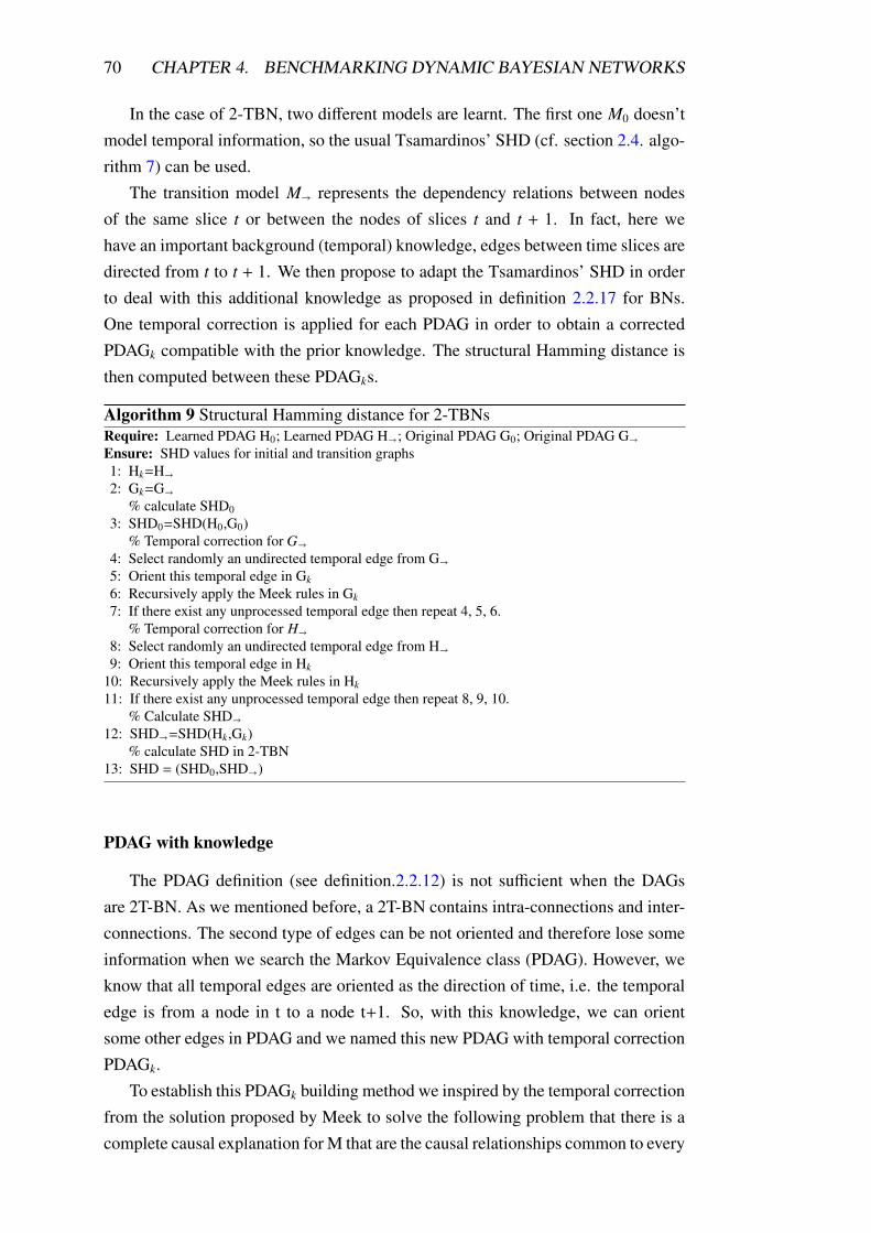
70 CHAPTER 4. BENCHMARKING DYNAMIC BAYESIAN NETWORKS
In the case of 2-TBN, two different models are learnt. The first one M0 doesn’t
model temporal information, so the usual Tsamardinos’ SHD (cf. section 2.4. algo-
rithm 7) can be used.
The transition model M� represents the dependency relations between nodes
of the same slice t or between the nodes of slices t and t + 1. In fact, here we
have an important background (temporal) knowledge, edges between time slices are
directed from t to t + 1. We then propose to adapt the Tsamardinos’ SHD in order
to deal with this additional knowledge as proposed in definition 2.2.17 for BNs.
One temporal correction is applied for each PDAG in order to obtain a corrected
PDAGk compatible with the prior knowledge. The structural Hamming distance is
then computed between these PDAGks.
Algorithm 9 Structural Hamming distance for 2-TBNs
Require: Learned PDAG H0; Learned PDAG H�; Original PDAG G0; Original PDAG G�
Ensure: SHD values for initial and transition graphs
1: Hk=H�
2: Gk=G�
% calculate SHD0
3: SHD0=SHD(H0,G0)
% Temporal correction for G�
4: Select randomly an undirected temporal edge from G�
5: Orient this temporal edge in Gk
6: Recursively apply the Meek rules in Gk
7: If there exist any unprocessed temporal edge then repeat 4, 5, 6.
% Temporal correction for H�
8: Select randomly an undirected temporal edge from H�
9: Orient this temporal edge in Hk
10: Recursively apply the Meek rules in Hk
11: If there exist any unprocessed temporal edge then repeat 8, 9, 10.
% Calculate SHD�
12: SHD�=SHD(Hk,Gk)
% calculate SHD in 2-TBN
13: SHD = (SHD0,SHD�)
PDAG with knowledge
The PDAG definition (see definition.2.2.12) is not sufficient when the DAGs
are 2T-BN. As we mentioned before, a 2T-BN contains intra-connections and inter-
connections. The second type of edges can be not oriented and therefore lose some
information when we search the Markov Equivalence class (PDAG). However, we
know that all temporal edges are oriented as the direction of time, i.e. the temporal
edge is from a node in t to a node t+1. So, with this knowledge, we can orient
some other edges in PDAG and we named this new PDAG with temporal correction
PDAGk.
To establish this PDAGk building method we inspired by the temporal correction
from the solution proposed by Meek to solve the following problem that there is a
complete causal explanation for M that are the causal relationships common to every
4.3. EVALUATION OF K-TBN GENERATED BY DATA AND PRIOR KNOWLEDGE71
complete causal explanation consistent with respect to the background knowledge
K?
To construct this PDAGk graph we have to follow three steps. (1) Construct the
PDAG, for this step we have used the Meek approach optimized by Chickering (cf.
section 2.2.4); (2) insert the temporal knowledge K, using the solution proposed
by Meek to insert the background knowledge (the set of directed edges which are
forbidden, the set of directed edges which are required). (3) apply Meek’s four
orientation rules (described in definition 2.2.17)
Proposition 4.3.1 (PDAG with temporal knowledge) [100]
Two 2T-BN structures are said to be equivalent if the set of distributions and tem-
poral constraints that can be represented with one of those structures is identical
to the set of distributions and temporal constraints that can be represented with the
other.
We notice that, we can use the same principal to calculate the SHD for k-TBN,
but we have to respect the definitions of intial and transition networks.
SHD(2T-BN) advantages
As we previously presented, the SHD for 2T-BN is a measure inspired from
SHD metric in the static case. So, all the SHD advantages are advantages charac-
terizing the SHD(2T-BN). In addition, the new SHD has other advantages when it
is used in the temporal (dynamic) case.
SHD advantages in the static context:
– It uses a reference model to evaluate contrary to the evaluation techniques
that use data. These are not reliable when there is little data;
– It is defined by the distance between two PDAGs and not between two DAGs;
With this method the problem of differences in orientation between the two
graphs in the same equivalence class are counted as errors is removed;
– It uses the hamming distance, which is simple to compute. It can maintain its
performance when the number of variables is large;
– It doesn’t use certain assumptions or conditions in calculating;
SHD advantages in the temporal context:
– It inserts the priori knowledge;
– It can run with large Dynamic Bayesian network;
– It uses the equivalence class to evalute, contrary to other metrics used in struc-
ture learning DBN studies (mentionned in section 3.4.2) as the method based
on sensitivity and specificity;
– It uses the temporal correction to construct PDAGk (see section 2.2.17;
72 CHAPTER 4. BENCHMARKING DYNAMIC BAYESIAN NETWORKS
4.4 Validation examples
4.4.1 2-TBN Benchmark generation
Implementation
The TileBN algorithm is implemented in Mathworks Matlab and is published as
part of the Causal Explorer system 1. The input BN is specified in HUGIN format,
and a simple parser was written to read HUGIN BNs in a custom Matlab format.
The measure of evaluation used by many BN learning algorithm is plotted over
several networks. Specifically, the following networks were used in the analysis,
listed in order to increase the number of variables (number of variables given in
parenthesis): Asia(8), Child (20), Insurance (27), Mildew (35), Alarm (37), Barley
(48), and HailFinder (56). These BN learning algorithms are compared to differ-
ent networks that contain 1, 3, 5, and 10 tiles of the original networks mentioned
previously.
For our implementation, we decided that the initial network M is provided in
Hugin 2 format readable by several BN software such as Genie/Smile 3 or Matlab
toolboxes such as Causal Explorer 4.
As we mentioned previously, our method is inspired from tiling BN of Tsamardi-
nos. So, we implement our method on the same tool used by tiling approach which
is matlab (causal explorer) but we used some other tools as genie/smile. The im-
plementation details of our method are shown in appendix B.
As Causal Explorer also proposes an implementation of bn tiling(), this func-
tion allows generating a tiled standard network consisting of N copies of tiles with
given connectivity parameter. We implemented our 2-TBN benchmark generation
in Matlab using this function, and added another function in order to export an un-
rolled 2-TBN model in Hugin format. This exported 2-TBN function can then be
used by several softwares for data generation and structure learning.
Toy example
Figure 4.2 illustrates our algorithm with ASIA [59] generating network, tiled 3
times for the initial model, with a maximum connectivity equal to 3. As we can see,
we are now able to generate realistic 2-TBNs with very large domains by choosing
any static and well-known benchmarks and controlling the complexity by increasing
the number of tiles.
We recommend the reader to consult our Web page for Dynamic Bayesian
1. http://www.dsl-lab.org/causal explorer
2. http://www.hugin.com/
3. http://genie.sis.pitt.edu/
4. http://www.dsl-lab.org/causal explorer/index.html
4.4. VALIDATION EXAMPLES 73
Figure 4.2: An example output of the 2-TBN generation algorithm. The generating
network is ASIA benchmark [59] shown in the top left of figure a). a) The output
of the initial network consists of three tiles of Asia with the addition of several in-
traconnecting edges shown with the dashed edges. b) The transition network output
together with several added interconnecting edges are shown with the dashed red
edges.
Networks # vars # edges Temporal # states # parents # neighbors
edges (min-Max) (min-Max) (min-Max)
Asia G0 8 8 2-2 0-2 1-4
Asia G� 16 21 5 2-2 0-3 1-5
Alarm G0 37 46 2-4 0-4 1-6
Alarm G� 74 110 18 2-4 0-4 1-7
Hailfinder G0 56 66 2-11 0-4 1-7
Hailfinder G� 112 156 24 2-11 0-4 1-17
Win95pts G0 76 112 2-2 0-7 1-10
Win95pts G� 156 256 41 2-2 0-7 1-10
Andes G0 223 338 2-2 0-6 1-12
Andes G� 446 820 144 2-2 0-6 1-12
Link G0 724 1125 2-4 0-3 1-17
Link G� 1448 2530 280 2-4 0-4 1-17
Table 4.1: Generated benchmarks for Dynamic Bayesian Network
Network benchmarking (https://sites.google.com/site/dynamicbencmharking/). We
present all standard large benchmarks for DBN that were constructed by our method
for tempral tiling (see table 4.1).
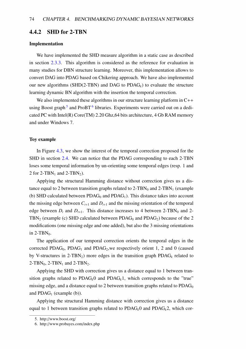
74 CHAPTER 4. BENCHMARKING DYNAMIC BAYESIAN NETWORKS
4.4.2 SHD for 2-TBN
Implementation
We have implemented the SHD measure algorithm in a static case as described
in section 2.3.3. This algorithm is considered as the reference for evaluation in
many studies for DBN structure learning. Moreover, this implementation allows to
convert DAG into PDAG based on Chikering approach. We have also implemented
our new algorithms (SHD(2-TBN) and DAG to PDAGk) to evaluate the structure
learning dynamic BN algorithm with the insertion the temporal correction.
We also implemented these algorithms in our structure learning platform in C++
using Boost graph 5 and ProBT 6 libraries. Experiments were carried out on a dedi-
cated PC with Intel(R) Core(TM) 2.20 Ghz,64 bits architecture, 4 Gb RAM memory
and under Windows 7.
Toy example
In Figure 4.3, we show the interest of the temporal correction proposed for the
SHD in section 2.4. We can notice that the PDAG corresponding to each 2-TBN
loses some temporal information by un-orienting some temporal edges (resp. 1 and
2 for 2-TBN1 and 2-TBN2).
Applying the structural Hamming distance without correction gives us a dis-
tance equal to 2 between transition graphs related to 2-TBN0 and 2-TBN1 (example
(b) SHD calculated between PDAG0 and PDAG1). This distance takes into account
the missing edge between Ct+1 and Dt+1 and the missing orientation of the temporal
edge between Dt and Dt+1. This distance increases to 4 between 2-TBN0 and 2-
TBN2 (example (c) SHD calculated between PDAG0 and PDAG2) because of the 2
modifications (one missing edge and one added), but also the 3 missing orientations
in 2-TBN0.
The application of our temporal correction orients the temporal edges in the
corrected PDAG0, PDAG1 and PDAG2,we respectively orient 1, 2 and 0 (caused
by V-structures in 2-TBN2) more edges in the transition graph PDAGk related to
2-TBN0, 2-TBN1 and 2-TBN2.
Applying the SHD with correction gives us a distance equal to 1 between tran-
sition graphs related to PDAGk0 and PDAGk1, which corresponds to the ”true”
missing edge, and a distance equal to 2 between transition graphs related to PDAG0
and PDAG1 (example (b)).
Applying the structural Hamming distance with correction gives us a distance
equal to 1 between transition graphs related to PDAGk0 and PDAGk2, which cor-
5. http://www.boost.org/
6. http://www.probayes.com/index.php
4.5. CONCLUSION 75
Figure 4.3: Examples of structural Hamming distance with or without temporal correction.
A first 2-TBN and its corresponding PDAG and corrected PDAG k are shown in (a). (b)
and (c) show another 2-TBN and their corresponding PDAG, and the structural Hamming
distance with the first model
responds to the ”true” missing edge, and a distance equal to 4 between transition
graphs related to PDAG0 and PDAG2 (example (c)).
As we can see in these toy examples, that our SHD with temporal correction
is better in term of structural comparison of dynamic bayesian networks. The im-
provement is given by the integration of knowledge (temporal knowledge) in our
metric.
4.5 Conclusion
We focused in this chapter on providing tools for benchmarking dynamic Bayesian
network structure learning algorithms. Our first contribution is a 2-TBN generation
algorithm inspired from the Tiling technique proposed by [95]. Our algorithm is
able to generate large and realistic 2-TBNs that can, then, be used for sampling
datasets. These datasets can then feed any 2-TBN structure learning algorithm.

76 CHAPTER 4. BENCHMARKING DYNAMIC BAYESIAN NETWORKS
Our second contribution is a novel metric for evaluating the performance of
these structure learning algorithms, by correcting the Structural Hamming distance
proposed by [104] in order to take into account temporal background information.
We have proposed a website by providing some 2-TBNs benchmarks (graphs
and datasets) in order to afford common evaluation tools for every researcher inter-
ested in 2-TBN structure learning 7.
7. https://sites.google.com/site/dynamicbencmharking/
5Dynamic Max Min Hill Climbing
(DMMHC)
Sommaire
5.1 Introduction . . . . . . . . . . . . . . . . . . . . . . . . . . . 79
5.2 Dynamic Max Min Parents and children DMMPC . . . . . . 79
5.2.1 Naıve DMMPC (neighborhood identification) . . . . . 80
Initial model . . . . . . . . . . . . . . . . . . . 80
Transition model . . . . . . . . . . . . . . . . . 80
5.2.2 Optimized DMMPC (Neighborhood identification) . . . 81
Initial model . . . . . . . . . . . . . . . . . . . 81
Transition model . . . . . . . . . . . . . . . . . 81
5.2.3 Toy example (naive DMMPC vs optimised DMMPC) . 83
5.2.4 Symmetrical correction . . . . . . . . . . . . . . . . . . 84
5.3 Dynamic Max Min Hill-Climbing DMMHC . . . . . . . . . . 85
5.4 DMMHC for simplified 2-TBN . . . . . . . . . . . . . . . . . 87
Neighborhood identification . . . . . . . . . . . 87
Symmetrical correction . . . . . . . . . . . . . . 88
DMMHC . . . . . . . . . . . . . . . . . . . . . 88
5.5 Time complexity of the algorithms . . . . . . . . . . . . . . . 88
Naive DMMHC . . . . . . . . . . . . . . . . . . 89
Optimised DMMHC . . . . . . . . . . . . . . . 89
Simplified DMMHC . . . . . . . . . . . . . . . 89
5.6 Related work . . . . . . . . . . . . . . . . . . . . . . . . . . . 90
77

78 CHAPTER 5. DYNAMIC MAX MIN HILL CLIMBING (DMMHC)
5.7 Conclusion . . . . . . . . . . . . . . . . . . . . . . . . . . . . 90
5.1. INTRODUCTION 79
5.1 Introduction
In this chapter, we focused on DBN structure learning with local search meth-
ods, by adapting the MMHC algorithm proposed by [104], one of the ”state of the
art” of this family algorithms . We believe that these local search algorithms can
easily take into account the temporal dimension. Our objective is to propose a gen-
eral structure learning algorithm that can work on 2-TBN models (with large search
space) and use large benchmarks for validation tests.
We first present a version of DMMHC which is a simple adaptation of MMHC
algorithm on 2-TBN models in section 5.2.1. Then, we optimized our approach
by the use of temporal constraints in section 5.2.2. In addition we defined another
version of the DMMHC that can run on simplified k-TBN models in section 5.4.
We described, the complexity of each version of the DMMHC in section 5.5 and
enumerated the advantages and disadvantages of our approach compared to others
existing approaches in literature.
5.2 Dynamic Max Min Parents and children DMMPC
In 2T-BN models, temporality is limited by the first order Markov assumption.
We think that local search algorithms can easily take into account this temporal
constraint. We propose here a new DBN structure learning algorithm inspired from
local search methods, by adapting the MMHC algorithm described in the previous
section.
As seen in section 3.2, the 2-TBN structure is defined by two independent graphs
G0 and G�. Inspired from the MMHC algorithm detailed in section 2.3.3, our Dy-
namic MMHC algorithm proposes to identify independently these graphs by apply-
ing a greedy search algorithm (adapted by [32] for 2T-BN) constrained with local
informations. This information is provided by the identification of the neighbor-
hood Ne0 (resp. Ne+) of each node in G0 (resp. G�).
By mimicking the procedure decomposition of MMHC described in section
2.3.3 , our local structure identification DMMPC will be decomposed into two tasks:
the neighborhood identification itself (DMMPC) completed by a symmetrical cor-
rection. We notice here that because of the non-symmetry of temporality, our local
structure identification will be able to automatically detect some directed parent or
children relationships if corresponding variables do not belong to the same time
slice.
The following sub-sections described separately each of the proposed proce-
dures, from the inner ones (the naive DMMPC, the optimised DMMPC and DMMPC)
to the final one (DMMHC).
80 CHAPTER 5. DYNAMIC MAX MIN HILL CLIMBING (DMMHC)
5.2.1 Naıve DMMPC (neighborhood identification)
Our DMMPC algorithm consists of two phases detailed in Algorithm 10 dedi-
cated to the identification of the neighborhood Ne0 (resp. Ne+) of a target variable
T in G0 (resp. G�).
Initial model X[0] and X[1] respectively denote the variables X for t = 0 and
t = 1. We remind that the 2T-BN model is first-order Markov. Hence, it is possible
that the neighborhood Ne0 of a variable T in X[0] can belong to X[0] and X[1].
Let us define CPC0 the parents or children of T in slice 0 and CC1 the children
of T in slice 1.
In DMMPC, we propose to use the static MMPC algorithm with the candidate
variables ListC0 =X[0] ∪X[1] \{T } in order to identify Ne0. Ne0 contains variables
included in ListC0. We notice that, in this case, the MaxMinHeuristic function
returns the maximum over all variables of the minimum association with T relative
to Ne0 (found), and the variable that belongs to ListC0 that achieves the maximum.
Because of temporal information, we will then be able to separate Ne0 = CPC0 ∪
CC1.
Transition model In the same way, X[t-1], X[t] and X[t + 1] respectively denote
the variables X for times t − 1, t and t + 1.
Ne+ of a variable T in X[t] can belong to X[t − 1], X[t] and X[t + 1]. So let us
define CPCt the parents or children of T in slice t, CCt+1 the children of T in slice
t + 1 and CPt−1 the parents of T in slice t − 1
We propose to use the static MMPC algorithm with the candidate variables
ListC = X[t − 1] ∪ X[t] ∪ X[t + 1]\{T } in order to identify Ne+ . We notice that,
in this case, the MaxMinHeuristic function returns the maximum over all variables
of the minimum association with T relative to Ne+ (found), and the variable that
belongs to ListC that achieves the maximum. Because of temporal information, we
will then be able to separate Ne+ = CPCt ∪CCt+1 ∪CPt−1.
Algorithm 10 DMMPC(T,D)
Require: target variable (T ); Data (D)
Ensure: neighborhood of T in G0 (Ne0) and in G� (Ne+)
% search Ne0 of T in t = 0
1: ListC0 = X[0]\{T }∪
X[1]
2: Ne0 =MMPC(T,D, ListC0)
% search Ne+ of T in t > 0
3: ListC = X[t-1]∪
X[t] \{T }∪
X[t+1]
4: Ne+ =MMPC(T,D, ListC)
5.2. DYNAMIC MAX MIN PARENTS AND CHILDREN DMMPC 81
5.2.2 Optimized DMMPC (Neighborhood identification)
The purpose of the following subsection is to redefine the previous method by
reducing the computational complexity result of section 5.2.1. To this end, we relied
on some properties:
– 2-TBN model is a first Markov order: the neighborhoods of a node in t time
slice belongs to 3 time slices (t-1, t, t+1).
– The orientations of all temporal edges are from t-1 to t time slices or from t
to t+1 time slices.
– The identification of these neighborhoods can be done in 3 steps: identifica-
tion of CPCt then CPt−1 then CCt−1 (this property is proposed by this thesis,
we give its proof later in the appendix C)
Initial model As mentioned in section 3.2.2, the initial model is a static BN rep-
resenting the initial joint distribution of the process P(X[t = 0]) and consisting of a
direct acyclic graph (DAG) G0 containing the variables X[t = 0].
In this case, it is not needful to identify the temporal dependences (with X[t =
1]) which concern only the transition model. For this reason, we propose in this
optimized version using the static MMPC algorithm with the candidate variables
ListC0 = X[0]\{T} (instead of X[0] ∪ X[1]\{T}) in order to restrict this step to the
identification of the neighborhoods Ne0 of a variable T in this specific time slice
X[0].
Transition model In this case, X[t-1], X[t] and X[t+1] respectively denote the
variables X for times t-1; t and t+1. Let us define CPCt the parents or children of T
in slice t, CCt+1 the children of T in slice t + 1 and CPt−1 the parents of T in slice
t - 1. According to the proposition 5.2.1 (the proof of this propostion given by the
appendix C), contrary to the naive method we will separate the set of Ne+ on CPCt,
CCt+1 and CPt−1 of a variable T in X[t]. Our algorithm tries to find the candidate
parents and/or children through separate steps.
In the first step, we start by a forward phase that searches for the candidates
that belong to CPCt using the static MMPC algorithm with the candidate variables
ListCt =X[t]\{T }. We notice that, the MaxMinHeuristic function returns the maxi-
mum over all variables of the minimum association with T relative to CPCt (found),
and X the variable that belongs to ListCt that achieves the maximum. The second
Backward phase will reveal if there is any independence between every S variable
in CPCt and T knowing all subsets in CPCt, and if it is true, this phase will remove
S from the CPCt as a false positive.
In the second step, we start by a forward phase that searches the candidates
that belong to CPt−1 using the static MMPC algorithm with the candidate variables
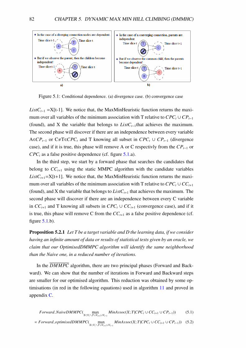
82 CHAPTER 5. DYNAMIC MAX MIN HILL CLIMBING (DMMHC)
Figure 5.1: Conditional dependence. (a) divergence case. (b) convergence case
ListCt−1 =X[t-1]. We notice that, the MaxMinHeuristic function returns the maxi-
mum over all variables of the minimum association with T relative to CPCt ∪CPt−1
(found), and X the variable that belongs to ListCt−1that achieves the maximum.
The second phase will discover if there are an independence between every variable
A∈CPt−1 or C,T∈CPCt and T knowing all subset in CPCt ∪ CPt−1 (divergence
case), and if it is true, this phase will remove A or C respectivly from the CPt−1 or
CPCt as a false positive dependence (cf. figure 5.1.a).
In the third step, we start by a forward phase that searches the candidates that
belong to CCt+1 using the static MMPC algorithm with the candidate variables
ListCt+1=X[t+1]. We notice that, the MaxMinHeuristic function returns the maxi-
mum over all variables of the minimum association with T relative to CPCt ∪CCt+1
(found), and X the variable that belongs to ListCt+1 that achieves the maximum. The
second phase will discover if there are an independence between every C variable
in CCt+1 and T knowing all subsets in CPCt ∪ CCt+1 (convergence case), and if it
is true, this phase will remove C from the CCt+1 as a false positive dependence (cf.
figure 5.1.b).
Proposition 5.2.1 Let T be a target variable and D the learning data, if we consider
having an infinite amount of data or results of statistical tests given by an oracle, we
claim that our OptimisedDMMPC algorithm will identify the same neighborhood
than the Naive one, in a reduced number of iterations.
In the DMMPC algorithm, there are two principal phases (Forward and Back-
ward). We can show that the number of iterations in Forward and Backward steps
are smaller for our optimised algorithm. This reduction was obtained by some op-
timisations (in red in the following equations) used in algorithm 11 and proved in
appendix C.
Forward NaiveDMMPC( maxX⊂Vt�T∪Vt+1∪Vt−1
MinAssoc(X; T |CPCt ∪CCt+1 ∪CPt−1)) (5.1)
⋍ Forward optimisedDMMPC( maxX⊂Vt�T∪Vt+1∪Vt−1
MinAssoc(X; T |CPCt ∪CCt+1 ∪CPt−1)) (5.2)
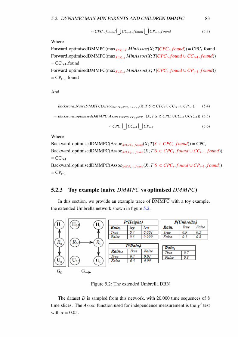
5.2. DYNAMIC MAX MIN PARENTS AND CHILDREN DMMPC 83
⋍ CPCt f ound∪
CCt+1 f ound∪
CPt−1 f ound (5.3)
Where
Forward optimisedDMMPC(maxX⊂Vt�T MinAssoc(X; T |CPCt f ound))=CPCt found
Forward optimisedDMMPC(maxX⊂Vt+1MinAssoc(X; T |CPCt f ound ∪CCt+1 f ound))
= CCt+1 found
Forward optimisedDMMPC(maxX⊂Vt−1MinAssoc(X; T |CPCt f ound ∪CPt−1 f ound))
= CPt−1 found
And
Backward NaiveDMMPC(AssocX∈CPCt∪CCt+1∪CPt−1(X; T |S ⊂ CPCt ∪CCt+1 ∪CPt−1)) (5.4)
⋍ Backward optimisedDMMPC(AssocX∈CPCt∪CCt+1∪CPt−1(X; T |S ⊂ CPCt∪CCt+1∪CPt−1)) (5.5)
⋍ CPCt
∪CCt+1
∪CPt−1 (5.6)
Where
Backward optimisedDMMPC(AssocX∈CPCt f ound(X; T |S ⊂ CPCt f ound)) = CPCt
Backward optimisedDMMPC(AssocX∈CCt+1 f ound(X; T |S ⊂ CPCt f ound ∪CCt+1 f ound))
= CCt+1
Backward optimisedDMMPC(AssocX∈CPt−1 f ound(X; T |S ⊂ CPCt f ound ∪CPt−1 f ound))
= CPt−1
5.2.3 Toy example (naive DMMPC vs optimised DMMPC)
In this section, we provide an example trace of DMMPC with a toy example,
the extended Umbrella network shown in figure 5.2.
Figure 5.2: The extended Umbrella DBN
The dataset D is sampled from this network, with 20.000 time sequences of 8
time slices. The Assoc function used for independence measurement is the χ2 test
with α = 0.05.
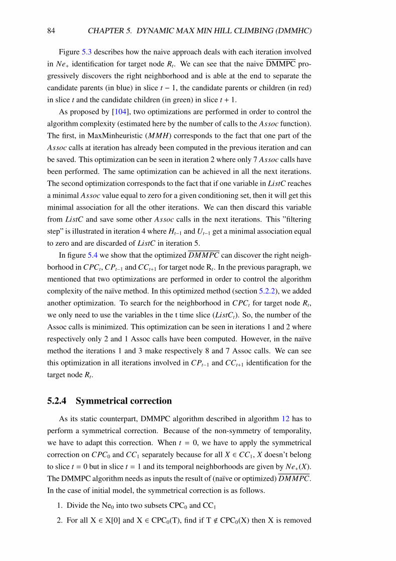
84 CHAPTER 5. DYNAMIC MAX MIN HILL CLIMBING (DMMHC)
Figure 5.3 describes how the naive approach deals with each iteration involved
in Ne+ identification for target node Rt. We can see that the naive DMMPC pro-
gressively discovers the right neighborhood and is able at the end to separate the
candidate parents (in blue) in slice t − 1, the candidate parents or children (in red)
in slice t and the candidate children (in green) in slice t + 1.
As proposed by [104], two optimizations are performed in order to control the
algorithm complexity (estimated here by the number of calls to the Assoc function).
The first, in MaxMinheuristic (MMH) corresponds to the fact that one part of the
Assoc calls at iteration has already been computed in the previous iteration and can
be saved. This optimization can be seen in iteration 2 where only 7 Assoc calls have
been performed. The same optimization can be achieved in all the next iterations.
The second optimization corresponds to the fact that if one variable in ListC reaches
a minimal Assoc value equal to zero for a given conditioning set, then it will get this
minimal association for all the other iterations. We can then discard this variable
from ListC and save some other Assoc calls in the next iterations. This ”filtering
step” is illustrated in iteration 4 where Ht−1 and Ut−1 get a minimal association equal
to zero and are discarded of ListC in iteration 5.
In figure 5.4 we show that the optimized DMMPC can discover the right neigh-
borhood in CPCt, CPt−1 and CCt+1 for target node Rt. In the previous paragraph, we
mentioned that two optimizations are performed in order to control the algorithm
complexity of the naıve method. In this optimized method (section 5.2.2), we added
another optimization. To search for the neighborhood in CPCt for target node Rt,
we only need to use the variables in the t time slice (ListCt). So, the number of the
Assoc calls is minimized. This optimization can be seen in iterations 1 and 2 where
respectively only 2 and 1 Assoc calls have been computed. However, in the naıve
method the iterations 1 and 3 make respectively 8 and 7 Assoc calls. We can see
this optimization in all iterations involved in CPt−1 and CCt+1 identification for the
target node Rt.
5.2.4 Symmetrical correction
As its static counterpart, DMMPC algorithm described in algorithm 12 has to
perform a symmetrical correction. Because of the non-symmetry of temporality,
we have to adapt this correction. When t = 0, we have to apply the symmetrical
correction on CPC0 and CC1 separately because for all X ∈ CC1, X doesn’t belong
to slice t = 0 but in slice t = 1 and its temporal neighborhoods are given by Ne+(X).
The DMMPC algorithm needs as inputs the result of (naıve or optimized) DMMPC.
In the case of initial model, the symmetrical correction is as follows.
1. Divide the Ne0 into two subsets CPC0 and CC1
2. For all X ∈ X[0] and X ∈ CPC0(T), find if T < CPC0(X) then X is removed
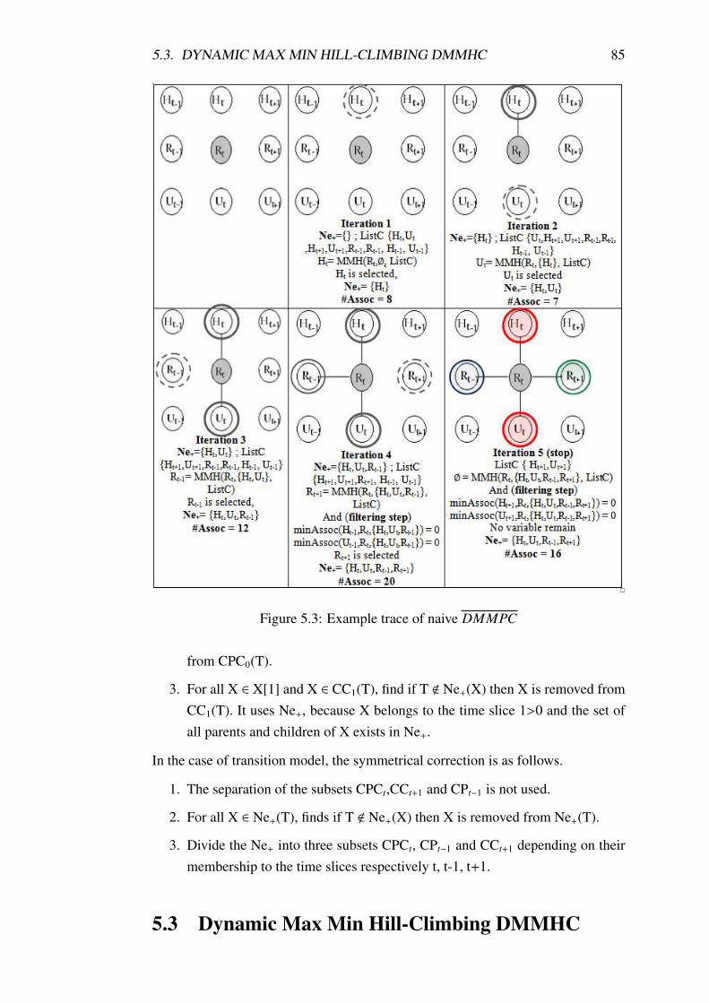
5.3. DYNAMIC MAX MIN HILL-CLIMBING DMMHC 85
Figure 5.3: Example trace of naive DMMPC
from CPC0(T).
3. For all X ∈ X[1] and X ∈ CC1(T), find if T < Ne+(X) then X is removed from
CC1(T). It uses Ne+, because X belongs to the time slice 1>0 and the set of
all parents and children of X exists in Ne+.
In the case of transition model, the symmetrical correction is as follows.
1. The separation of the subsets CPCt,CCt+1 and CPt−1 is not used.
2. For all X ∈ Ne+(T), finds if T < Ne+(X) then X is removed from Ne+(T).
3. Divide the Ne+ into three subsets CPCt, CPt−1 and CCt+1 depending on their
membership to the time slices respectively t, t-1, t+1.
5.3 Dynamic Max Min Hill-Climbing DMMHC
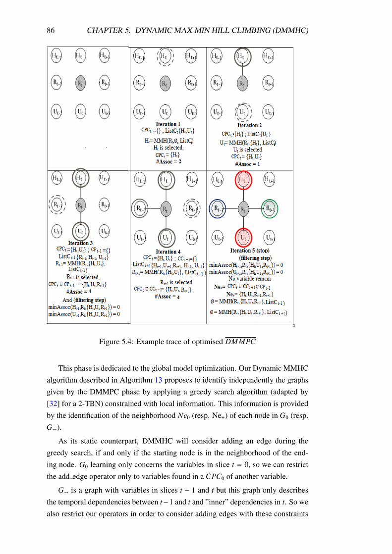
86 CHAPTER 5. DYNAMIC MAX MIN HILL CLIMBING (DMMHC)
Figure 5.4: Example trace of optimised DMMPC
This phase is dedicated to the global model optimization. Our Dynamic MMHC
algorithm described in Algorithm 13 proposes to identify independently the graphs
given by the DMMPC phase by applying a greedy search algorithm (adapted by
[32] for a 2-TBN) constrained with local information. This information is provided
by the identification of the neighborhood Ne0 (resp. Ne+) of each node in G0 (resp.
G�).
As its static counterpart, DMMHC will consider adding an edge during the
greedy search, if and only if the starting node is in the neighborhood of the end-
ing node. G0 learning only concerns the variables in slice t = 0, so we can restrict
the add edge operator only to variables found in a CPC0 of another variable.
G� is a graph with variables in slices t − 1 and t but this graph only describes
the temporal dependencies between t−1 and t and ”inner” dependencies in t. So we
also restrict our operators in order to consider adding edges with these constraints
5.4. DMMHC FOR SIMPLIFIED 2-TBN 87
and we don’t authorize reversing the temporal edges.
5.4 DMMHC for simplified 2-TBN
In simplified kT-BN , the temporality is constrained by the k order Markov as-
sumption. There are two cases for this model when k=2 and k≥3. The first case
is the simplified k-TBN. It allows representing the transition network with only
the inter-connectivity between t-1 and t time slices and we can apply the first or-
der Markov assumption in this model. We used this case in our work DMMHC
for simplified 2-TBN. The second case represents the transition network with the
inter-connectivity between t-s and t time slices where k > s.
We think that our DMMHC algorithm can easily take into account these tem-
poral constraints. We propose here an extension of DMMHC named simplified
DMMHC for 2-TBN structure learning.
As seen in section 3.2, the 2-TBN simplified structure focuses only on G�. This
kind of model is limited to contain only inter time slice arcs. Inspired by DMMHC
algorithm, our new simplified DMMHC algorithm proposes to identify G� graph
by applying the different phases of DMMHC shown in the previous sections.
Neighborhood identification In the first phase of neighborhood identification,
we need only to identify the Ne+ for all variables T in t time slice. As we previously
defined the set of Ne+(T)=CPt−1(T)∪
CPCt(T)∪
CCt+1(T). In the simplified 2-
TBN we have many properties to define (figure 5.5):
1. we don’t need to identify the CPCt(T) candidates because we are interested
in the inter connectivity only.
2. we don’t need to identify the CCt+1(T) candidates because if X ∈ CC(T)⇒ T
∈ CP(X) where X in t time slice (the temporal symmetrical correction result).
3. Ne+(T)= CPt−1(T)∪
CPCt(T)∪
CCt+1(T). We notice that with the use of the
properties 1 and 2⇒ Ne+(T)= CPt−1(T).
4. To identify all X in CPt−1(T), we need to compute the MaxMinAssoc(X;
T|CPt−1
∪CPCt). We suggested below the proposition 5.4.1 to facilate the
computation (the proof of this propostion given by the appendix C):
5. The Backward phase of DMMHC allows to detect any false positives depend-
ing on the structure. But after the Forward phase we musn’t find any one. So
we can remove the Backward phase in DMMHC simplified.
Proposition 5.4.1 Let Vt−1 the set of variables for time slice t-1 and X ∈ Vt−1.
maxX
min Assoc(X; T |Ne+(T )) = maxX
min Assoc(X; T |CPt−1) = maxX
Assoc(X; T |∅)
(5.7)
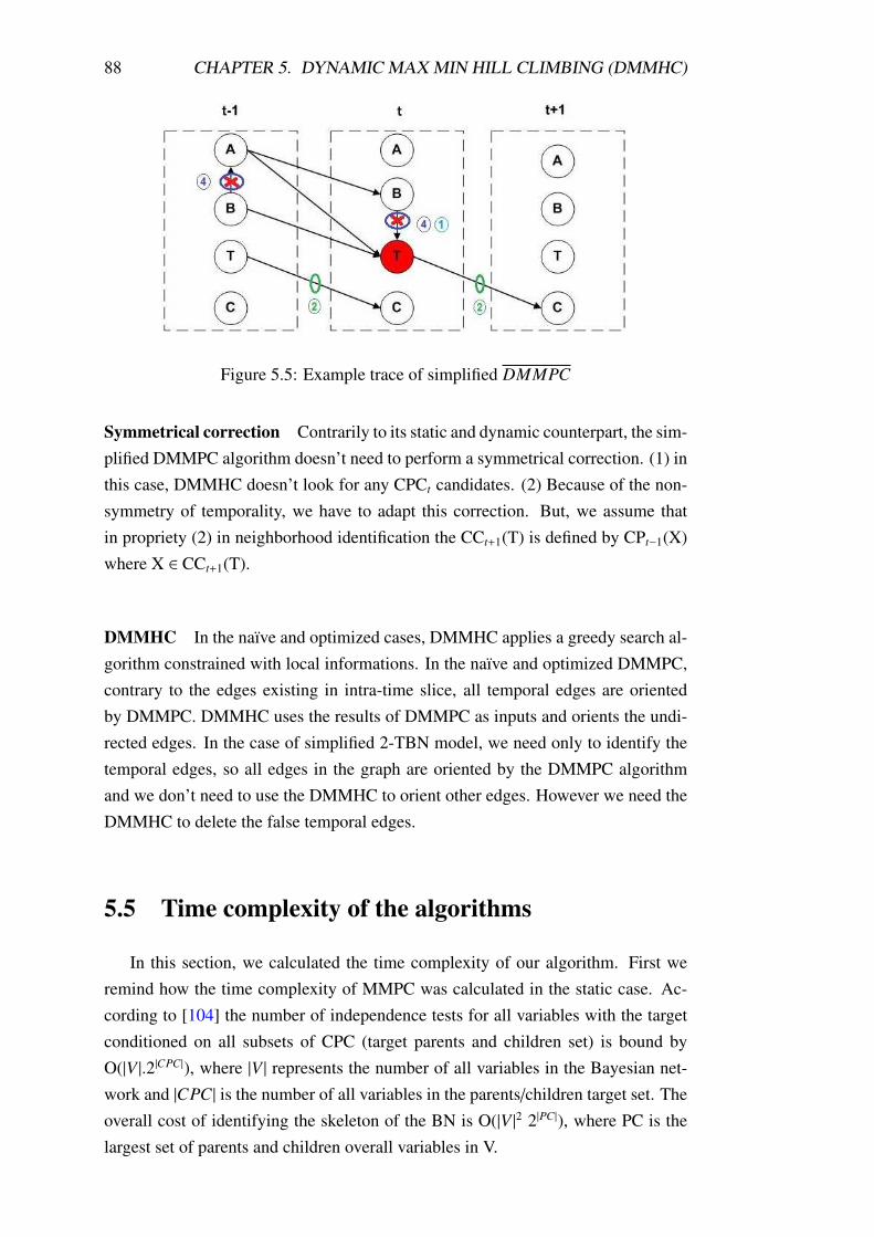
88 CHAPTER 5. DYNAMIC MAX MIN HILL CLIMBING (DMMHC)
Figure 5.5: Example trace of simplified DMMPC
Symmetrical correction Contrarily to its static and dynamic counterpart, the sim-
plified DMMPC algorithm doesn’t need to perform a symmetrical correction. (1) in
this case, DMMHC doesn’t look for any CPCt candidates. (2) Because of the non-
symmetry of temporality, we have to adapt this correction. But, we assume that
in propriety (2) in neighborhood identification the CCt+1(T) is defined by CPt−1(X)
where X ∈ CCt+1(T).
DMMHC In the naıve and optimized cases, DMMHC applies a greedy search al-
gorithm constrained with local informations. In the naıve and optimized DMMPC,
contrary to the edges existing in intra-time slice, all temporal edges are oriented
by DMMPC. DMMHC uses the results of DMMPC as inputs and orients the undi-
rected edges. In the case of simplified 2-TBN model, we need only to identify the
temporal edges, so all edges in the graph are oriented by the DMMPC algorithm
and we don’t need to use the DMMHC to orient other edges. However we need the
DMMHC to delete the false temporal edges.
5.5 Time complexity of the algorithms
In this section, we calculated the time complexity of our algorithm. First we
remind how the time complexity of MMPC was calculated in the static case. Ac-
cording to [104] the number of independence tests for all variables with the target
conditioned on all subsets of CPC (target parents and children set) is bound by
O(|V |.2|CPC|), where |V | represents the number of all variables in the Bayesian net-
work and |CPC| is the number of all variables in the parents/children target set. The
overall cost of identifying the skeleton of the BN is O(|V |2 2|PC|), where PC is the
largest set of parents and children overall variables in V.
5.5. TIME COMPLEXITY OF THE ALGORITHMS 89
Naive DMMHC In our dynamic (temporal) case, as for the static, we first identify
the number of tests in DMMPC. In this part we have two cases to present (i.e. t=0
and t>0). For t=0, DMMPC will calculate the association of all variables in time
slices t=0 and t=1 with target in slice t=0 conditioned on all subset of Ne0 (in the
worst case). Thus, the number of tests in the case t=0 is bounded by O(|2V |.2|Ne0 |),
where V is the set of all variables in a time slice. For t>0 case, the number of
tests is bounded by O((|3V |.2|Ne+ |), because DMMPC calculates the association of
all variables in three time slices t, t-1, t+1 with the target in slice t conditioned on
all subsets of Ne+ (in the worst case).
We sum up, the total number of tests in both phases at t = 0 and t > 0 is
bounded respectively by O(|2V |.2|Ne0 |) and O(|3V |.2|Ne+ |). Thus, the total number of
tests in both phases is bounded by O(|3V |.2|Ne+ |). The overall cost of identifying
the skeleton of the initial and transition models in dynamic Bayesian network (i.e.,
calling DMMPC with all targets in G0 and G� ) is O(|3V |2.2|Ne|), where Ne is the
largest set of neighborhood (in t and t+1 and t-1) over all variables in the time slice
t.
Optimised DMMHC For the optimized DMMPC, we start with t=0, DMMPC
will calculate the association of all variables in time slices t=0 with target in slice
t=0 conditioned on all subsets of CPC0 (in the worst case). Thus, the number of tests
in the case t=0 is bounded by O(|V |.2|CPC0 |), where V is the set of all variables in a
time slice. For t≥1 case, the number of tests is bounded by O(|V |.2|CPCt |+|V |.2|CPCt |+|CPt−1 |
+|V |.2|CPCt |+|CCt+1 |) , because DMMPC calculates the association of all variables in t
or in t-1 or t+1 with the target in slice t conditioned on all subsets respectively of
CPCt or CPCt ∪CPt−1 or CPCt ∪CCt+1 (in the worst case).
To recapitulate, the total number of tests in both phases at t = 0 and t ≻ 0 is
bounded respectively by O(|V |.2|CPC|) and O(|V |.22|CPC|), where CPC is the largest
set of neighborhood in one time slice (t or t+1 or t-1) over all variables in t (i.e.
|Ne| ≃ 3*|CPC|). Thus, the total number of tests in both phases is bounded by
O(|V |.22|CPC|). The overall cost of identifying the skeleton of initial and transition
models in dynamic Bayesian network (i.e., calling DMMPC with all targets in G0
and G�) is O(|V |2.22|CPC|).
Simplified DMMHC The simplified DMMHC deals with the transition model
only. DMMPC calculated the association of all variables in time slice t-1 with
target in slice t conditioned on empty set (in all cases). Thus, the number of tests in
the case t is bounded by O(N), where N is the set of all variables in a time slice.
We assume that, since we don’t need to use the symmetrical correction and
DMMHC, the overall cost of identifying the skeleton of transition model in dynamic
Bayesian network (i.e., calling DMMPC with all targets in G�) is O(N2).
90 CHAPTER 5. DYNAMIC MAX MIN HILL CLIMBING (DMMHC)
5.6 Related work
Many approaches for structure learning in DBN [32, 107, 108, 35, 112] are
validated on benchmark models with about 10 variables. In a more general context,
due to inherent limitations of the score-based structure learning methods, all these
methods will have a very high complexity if the number of variables increases.
With the help of a local search, DMMHC is able to limit the search space in the
final global optimization (GS). In this way, we can theoritically work in high dimen-
sions like MMHC with static BNs. We can say that our approach outperforms the
other approaches based on score, because contrary to these last kind of approaches,
DMMHC can deal with large dimension and on complete search space.
Another way to deal with scalability is to restrict the class of 2T-BN by only
considering parents of Xi[t] in time slice t-1 (for 2T-BN) or any previous time slice
(for kT-BN).
Dojer [27] proposes a score based method named polynomial time algorithm
for learning this class of DBN (with BDe and MDL scores). Vinh et al. [111]
proposed another polynomial time algorithm in the same context (equicardinality
requirement) with other scoring function (MIT). Also, the authors proposed an-
other contribution in this work consisting of a hybrid method with local Blanket
identification (MIT-MMMB).
DMMHC and MIT based MMMB are both hybrid methods with local search
and global optimization. When DMMHC tries to identify the candidate parents/children
CPC set of a target variable in a 2T-BN, MIT based MMMB tries to identify the
(more complex) Markov Blanket MB but in a restricted subclass of 2T-BNs. On the
one hand, this assumption allows to simplify both MB discovery and global opti-
mization. On the other hand, contrary to DMMHC, MIT based MMMB is not able
to identify the intra-time dependencies. So, the hybrid method doesexist in liter-
ature and it can deal with large dimension but it is executed on simplified search
space. In addition, we have proposed another version of DMMHC which can work
on this kind of models.
5.7 Conclusion
In this chapter, we proposed a new 2T-BN structure learning algorithm dealing
with large networks. Inspired from the MMHC algorithm proposed by [104] for
static BNs, our DMMHC algorithm is a local search algorithm dealing with local
structure identification (DMMPC) and global model optimization constrained with
this local information.
We have shown that the local structure identification can easily take into account
the temporal dimension in order to provide some additional information about tem-
5.7. CONCLUSION 91
porality that can then be used with a greedy search in order to learn the global
structure, the initial model G0, and the transition one G�. As far as we know, no
method capable to learn 2-TBN models with such approaches has been proposed
previously.
We also presented an optimisation for our DMMHC named optimised DMMHC.
It is a local improvement of our algorithm. We think that our scalability can be
improved during the local structure identification using temporality constraints in
DMMPC in order to decrease the number of Assoc calls and consequently decrease
the running time that we will demonstrate in the next chapter dealing with our ex-
perimentation.
Furthmore, in this chapter, we suggested a new version of DMMHC, which
work on simplified 2-TBN without intra-connectivity edges. We compared all the
versions of DMMHC (naive DMMHC, optimised DMMHC and simplified DMMHC)
for 2T-BN structure learning in terms of complexity and showed that we are able to
decrease the complexity with the use of temporal constraints.

92 CHAPTER 5. DYNAMIC MAX MIN HILL CLIMBING (DMMHC)
Algorithm 11 DMMPCoptimised(T,D)
Require: target variable (T ); Data (D)
Ensure: neighborhood of T in G0 (Ne0) and in G� (Ne+)
% search Ne0 of T in t = 0
1: ListC0 = X[0]\ {T}
2: Ne0 =MMPC(T,D, ListC0)
% search Ne+ of T in t > 0
3: CPCt = ∅% parents children candidates for T in slice t
4: CPt−1 = ∅% only parents candidates for T in slice t-1
5: CCt+1 = ∅% only children candidates for T in slice t+1
% search Ne+ of T in t, t + 1 and t − 1
6: ListCt = X[t]\ {T}
7: ListCt+1 = X[t+1]\ {T}
8: ListCt−1 = X[t-1]\ {T}
% search CPCt
% Phase I: Forward
9: repeat
10: ≺ F, assocF ≻ =MaxMinHeuristic(T,CPCt, ListCt)
11: if assocF , 0 then
12: CPCt = CPCt
∪{F}
13: ListCt = ListCt \ {F}
14: end if
15: until CPCt has not change or assocF = 0 or ListCt = ∅
% Phase II: Backward
16: for all X ∈ CPCt do
17: if ∃S ⊆ CPCt and assoc(X; T |S ) = 0 then
18: CPC \ {X}
19: end if
20: end for
% search CPt−1
% Phase I: Forward
21: repeat
22: ≺ F, assocF ≻ =MaxMinHeuristic(T,CPCt ∪CPt−1, ListCt−1)
23: if assocF , 0 then
24: CPt−1 = CPt−1
∪{F}
25: ListCt−1 = ListCt−1 \ {F}
26: end if
27: until CPt−1 has not change or assocF = 0 or ListCt−1 = ∅
% Phase II: Backward
28: for all X ∈ CPCt ∪CPt−1 do
29: if ∃S ⊆ CPCt ∪CPt−1 and assoc(X; T |S ) = 0 then
30: CPt−1 \ {X} or CPCt \ {X}
31: end if
32: end for
% search CCt+1
% Phase I: Forward
33: repeat
34: ≺ F, assocF ≻ =MaxMinHeuristic(T,CPCt ∪CCt+1, ListCt+1)
35: if assocF , 0 then
36: CCt+1 = CCt+1
∪{F}
37: ListCt+1 = ListCt+1 \ {F}
38: end if
39: until CCt+1 has not change or assocF = 0 or ListCt+1 = ∅
% Phase II: Backward
40: for all X ∈ CCt+1 do
41: if ∃S ⊆ CPCt ∪CCt+1 and assoc(X; T |S ) = 0 then
42: CCt+1 \ {X}
43: end if
44: end for
45: Ne+= CPCt
∪CPt−1
∪CCt+1
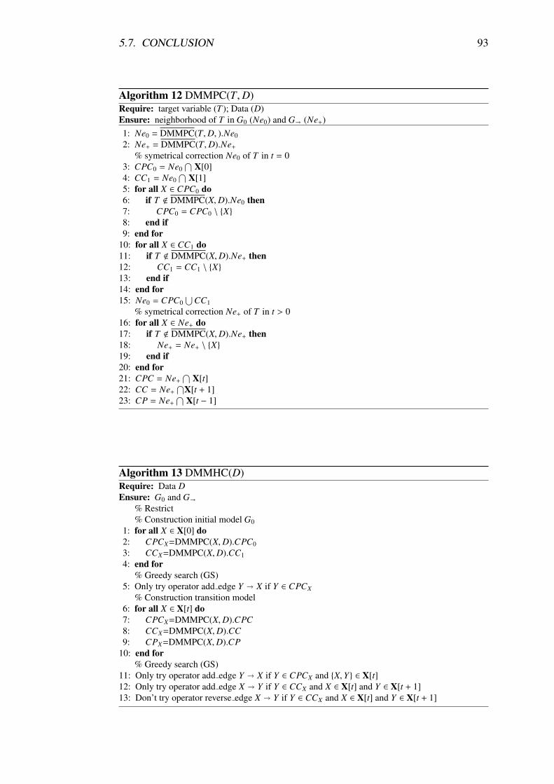
5.7. CONCLUSION 93
Algorithm 12 DMMPC(T,D)
Require: target variable (T ); Data (D)
Ensure: neighborhood of T in G0 (Ne0) and G� (Ne+)
1: Ne0 = DMMPC(T,D, ).Ne0
2: Ne+ = DMMPC(T,D).Ne+% symetrical correction Ne0 of T in t = 0
3: CPC0 = Ne0
∩X[0]
4: CC1 = Ne0
∩X[1]
5: for all X ∈ CPC0 do
6: if T < DMMPC(X,D).Ne0 then
7: CPC0 = CPC0 \ {X}
8: end if
9: end for
10: for all X ∈ CC1 do
11: if T < DMMPC(X,D).Ne+ then
12: CC1 = CC1 \ {X}
13: end if
14: end for
15: Ne0 = CPC0
∪CC1
% symetrical correction Ne+ of T in t > 0
16: for all X ∈ Ne+ do
17: if T < DMMPC(X,D).Ne+ then
18: Ne+ = Ne+ \ {X}
19: end if
20: end for
21: CPC = Ne+∩
X[t]
22: CC = Ne+∩
X[t + 1]
23: CP = Ne+∩
X[t − 1]
Algorithm 13 DMMHC(D)
Require: Data D
Ensure: G0 and G�
% Restrict
% Construction initial model G0
1: for all X ∈ X[0] do
2: CPCX=DMMPC(X,D).CPC0
3: CCX=DMMPC(X,D).CC1
4: end for
% Greedy search (GS)
5: Only try operator add edge Y � X if Y ∈ CPCX
% Construction transition model
6: for all X ∈ X[t] do
7: CPCX=DMMPC(X,D).CPC
8: CCX=DMMPC(X,D).CC
9: CPX=DMMPC(X,D).CP
10: end for
% Greedy search (GS)
11: Only try operator add edge Y � X if Y ∈ CPCX and {X,Y} ∈ X[t]
12: Only try operator add edge X � Y if Y ∈ CCX and X ∈ X[t] and Y ∈ X[t + 1]
13: Don’t try operator reverse edge X � Y if Y ∈ CCX and X ∈ X[t] and Y ∈ X[t + 1]

94 CHAPTER 5. DYNAMIC MAX MIN HILL CLIMBING (DMMHC)
Algorithm 14 DMMPCsimplified(T,D)
Require: target variable (T ); Data (D)
Ensure: neighborhood of T in G� (Ne+)
% search Ne+ of T in t > 0
1: CPt−1 = ∅% only parents candidates for T in slice t-1
% search Ne+ of T in t − 1
2: ListCt−1 = X[t-1]\ {T}
% search CPt−1
% Phase I: Forward
3: repeat
4: ≺ F, assocF ≻ =MaxAssoc(T, {}, ListCt−1)
5: if assocF , 0 then
6: CPt−1 = CPt−1
∪{F}
7: ListCt−1 = ListCt−1 \ {F}
8: end if
9: until CPt−1 has not change or assocF = 0 or ListCt−1 = ∅
10: Ne+= CPt−1
6Experimental study
Sommaire
6.1 Introduction . . . . . . . . . . . . . . . . . . . . . . . . . . . 96
6.2 Experimental protocol . . . . . . . . . . . . . . . . . . . . . . 96
6.2.1 Algorithms . . . . . . . . . . . . . . . . . . . . . . . . 96
6.2.2 Benchmarks . . . . . . . . . . . . . . . . . . . . . . . . 97
6.2.3 Performance indicators . . . . . . . . . . . . . . . . . . 97
6.3 Empirical results and interpretations on complete search space 98
6.3.1 Initial validation . . . . . . . . . . . . . . . . . . . . . 98
6.3.2 DMMHC versus dynamic GS and SA . . . . . . . . . . 99
6.3.3 Naive versus optimized DMMHC . . . . . . . . . . . . 102
6.4 Empirical results and interpretations on simplified search
space . . . . . . . . . . . . . . . . . . . . . . . . . . . . . . . 104
6.4.1 Simplified 2-TBN with small benchmark . . . . . . . . 104
6.4.2 Simplified 2-TBN with large benchmark . . . . . . . . . 107
6.5 Comparison between all DMMHC versions . . . . . . . . . . 108
6.6 Conclusion . . . . . . . . . . . . . . . . . . . . . . . . . . . . 110
95
96 CHAPTER 6. EXPERIMENTAL STUDY
6.1 Introduction
The experimental study presented in this chapter covered many points that pre-
sented in the previous chapters of our contributions. In this chapter, we were jus-
tified our theoretical ideas by real experiments. First, in section 6.2, we described
our experimental protocol. We explained the steps used to prepare the necessary
elements to run the experiments concerning the structure learning algorithms, the
small and large benchmarks used for evaluation and finally the different metrics
used to compare between different techniques presented in this thesis.
In section 6.3, we performed some experiments with our methods and others
techniques existing in literature on the same context, and we showed the different
results with their corresponding interpretations.
After that, in section 6.4 we mainly focused on the application of simplified
DMMHC to one biological and genetic task on simplified search space. We com-
pared our DMMHC algorithms with others tools available in the internet as Banjo,
BNFinder, etc... Finally, section 6.5 is dedicated to a scalability comparison of all
versions of DMMHC.
6.2 Experimental protocol
6.2.1 Algorithms
We have implemented the Greedy Search (GS) for 2T-BN as described in section
3.2. This algorithm is considered as the reference algorithm for DBN structure
learning. We have also implemented our proposal, DMMHC, described in chapter
5. We can notice here that our algorithm uses a constrained greedy search, whereas
the original MMHC algorithm proposes to use a Tabu search.
We can notice that the MMHC implementation available in our platform em-
ploys a chi-square test based on the χ2 statistics. Our implementation also uses a
standard formula to compute the degree of freedom instead of the heuristic proposed
in the original publication [103]. These differences may also explain some of the
discrepancy found when we are trying to reproduce the results from the literature.
In the greedy search, we used the BIC score function. χ2 independence test is
used with α = 0.05.
Experiments were carried out on a dedicated PC with Intel(R) Core(TM) 2.20
Ghz, 64 bits architecture, 4 Gb RAM memory and under Windows 7.
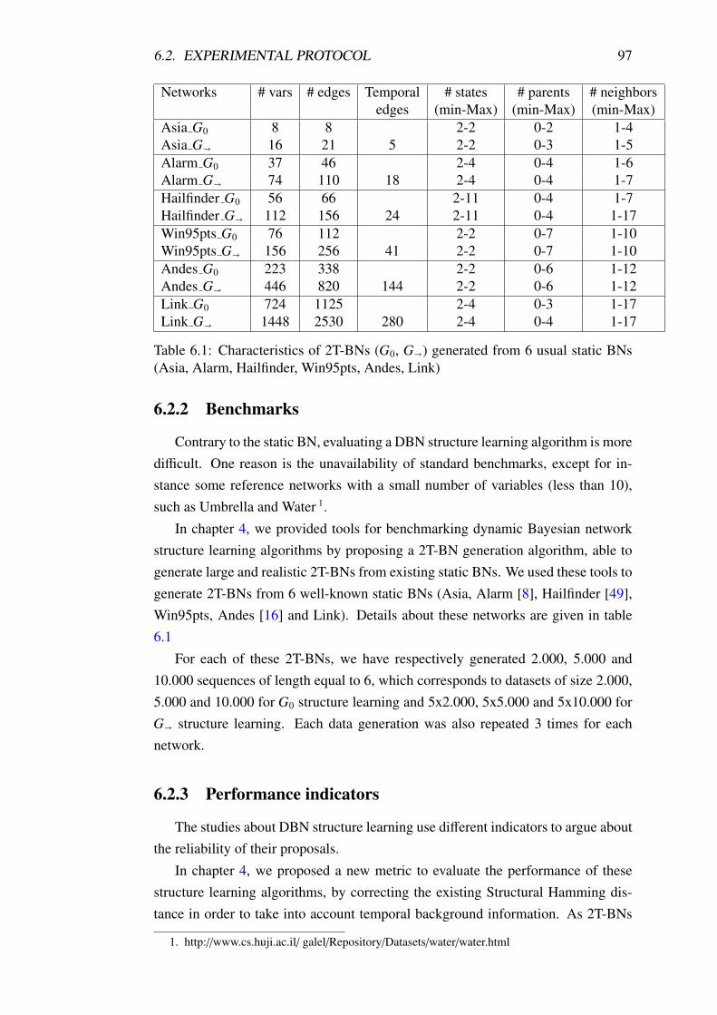
6.2. EXPERIMENTAL PROTOCOL 97
Networks # vars # edges Temporal # states # parents # neighbors
edges (min-Max) (min-Max) (min-Max)
Asia G0 8 8 2-2 0-2 1-4
Asia G� 16 21 5 2-2 0-3 1-5
Alarm G0 37 46 2-4 0-4 1-6
Alarm G� 74 110 18 2-4 0-4 1-7
Hailfinder G0 56 66 2-11 0-4 1-7
Hailfinder G� 112 156 24 2-11 0-4 1-17
Win95pts G0 76 112 2-2 0-7 1-10
Win95pts G� 156 256 41 2-2 0-7 1-10
Andes G0 223 338 2-2 0-6 1-12
Andes G� 446 820 144 2-2 0-6 1-12
Link G0 724 1125 2-4 0-3 1-17
Link G� 1448 2530 280 2-4 0-4 1-17
Table 6.1: Characteristics of 2T-BNs (G0, G�) generated from 6 usual static BNs
(Asia, Alarm, Hailfinder, Win95pts, Andes, Link)
6.2.2 Benchmarks
Contrary to the static BN, evaluating a DBN structure learning algorithm is more
difficult. One reason is the unavailability of standard benchmarks, except for in-
stance some reference networks with a small number of variables (less than 10),
such as Umbrella and Water 1.
In chapter 4, we provided tools for benchmarking dynamic Bayesian network
structure learning algorithms by proposing a 2T-BN generation algorithm, able to
generate large and realistic 2T-BNs from existing static BNs. We used these tools to
generate 2T-BNs from 6 well-known static BNs (Asia, Alarm [8], Hailfinder [49],
Win95pts, Andes [16] and Link). Details about these networks are given in table
6.1
For each of these 2T-BNs, we have respectively generated 2.000, 5.000 and
10.000 sequences of length equal to 6, which corresponds to datasets of size 2.000,
5.000 and 10.000 for G0 structure learning and 5x2.000, 5x5.000 and 5x10.000 for
G� structure learning. Each data generation was also repeated 3 times for each
network.
6.2.3 Performance indicators
The studies about DBN structure learning use different indicators to argue about
the reliability of their proposals.
In chapter 4, we proposed a new metric to evaluate the performance of these
structure learning algorithms, by correcting the existing Structural Hamming dis-
tance in order to take into account temporal background information. As 2T-BNs
1. http://www.cs.huji.ac.il/ galel/Repository/Datasets/water/water.html
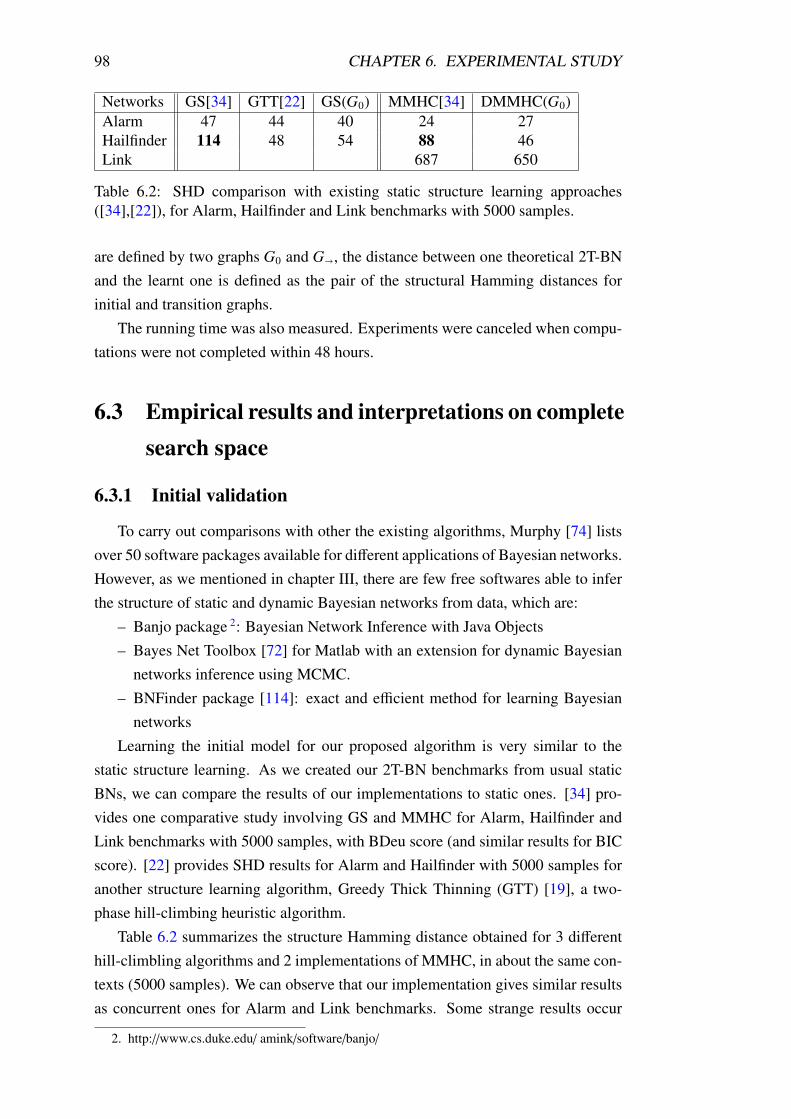
98 CHAPTER 6. EXPERIMENTAL STUDY
Networks GS[34] GTT[22] GS(G0) MMHC[34] DMMHC(G0)
Alarm 47 44 40 24 27
Hailfinder 114 48 54 88 46
Link 687 650
Table 6.2: SHD comparison with existing static structure learning approaches
([34],[22]), for Alarm, Hailfinder and Link benchmarks with 5000 samples.
are defined by two graphs G0 and G�, the distance between one theoretical 2T-BN
and the learnt one is defined as the pair of the structural Hamming distances for
initial and transition graphs.
The running time was also measured. Experiments were canceled when compu-
tations were not completed within 48 hours.
6.3 Empirical results and interpretations on complete
search space
6.3.1 Initial validation
To carry out comparisons with other the existing algorithms, Murphy [74] lists
over 50 software packages available for different applications of Bayesian networks.
However, as we mentioned in chapter III, there are few free softwares able to infer
the structure of static and dynamic Bayesian networks from data, which are:
– Banjo package 2: Bayesian Network Inference with Java Objects
– Bayes Net Toolbox [72] for Matlab with an extension for dynamic Bayesian
networks inference using MCMC.
– BNFinder package [114]: exact and efficient method for learning Bayesian
networks
Learning the initial model for our proposed algorithm is very similar to the
static structure learning. As we created our 2T-BN benchmarks from usual static
BNs, we can compare the results of our implementations to static ones. [34] pro-
vides one comparative study involving GS and MMHC for Alarm, Hailfinder and
Link benchmarks with 5000 samples, with BDeu score (and similar results for BIC
score). [22] provides SHD results for Alarm and Hailfinder with 5000 samples for
another structure learning algorithm, Greedy Thick Thinning (GTT) [19], a two-
phase hill-climbing heuristic algorithm.
Table 6.2 summarizes the structure Hamming distance obtained for 3 different
hill-climbling algorithms and 2 implementations of MMHC, in about the same con-
texts (5000 samples). We can observe that our implementation gives similar results
as concurrent ones for Alarm and Link benchmarks. Some strange results occur
2. http://www.cs.duke.edu/ amink/software/banjo/
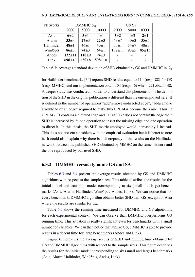
6.3. EMPIRICAL RESULTS AND INTERPRETATIONS ON COMPLETE SEARCH SPACE99
Networks DMMHC G0 GS G0
2000 5000 10000 2000 5000 10000
Asia 6±2 5±1 4±1 5±2 4±2 2±1
Alarm 33±3 27±3 22±3 43±7 40±3 35±5
Hailfinder 48±1 46±1 40±1 55±1 54±7 48±5
Win95pts 86±3 74±3 64±1 102±11 93±5 85±15
Andes 132±11 110±9 94±3 - - -
Link 698±13 650±8 598±10 - - -
Table 6.3: Average±standard deviation of SHD obtained by GS and DMMHC in G0
for Hailfinder benchmark. [34] reports SHD results equal to 114 (resp. 88) for GS
(resp. MMHC) and our implementation obtains 54 (resp. 46) when [22] obtains 48.
A deeper study was conducted in order to understand this phenomenon. The defini-
tion of the SHD in the original publication is different than the one employed here. It
is defined as the number of operations ”add/remove undirected edge”, ”add/remove
arrowhead of an edge” required to make two CPDAGs become the same. Thus, if
CPDAG G1 contains a directed edge and CPDAG G2 does not contain the edge their
SHD is increased by 2: one operation to insert the missing edge and one operation
to direct it. In this thesis, the SHD metric employed would increase by 1 instead.
This does not present a problem with the empirical evaluation but it is better to note
it. It could also explain why there is a discrepancy in the results on the Hailfinder
network between the published SHD obtained by MMHC on the same network and
the one reproduced by our used SHD.
6.3.2 DMMHC versus dynamic GS and SA
Tables 6.3 and 6.4 present the average results obtained by GS and DMMHC
algorithms with respect to the sample sizes. This table describes the results for the
initial model and transition model corresponding to six (small and large) bench-
marks (Asia, Alarm, Hailfinder, Win95pts, Andes, Link). We can notice that for
every benchmark, DMMHC algorithm obtains better SHD than GS. except for Asia
where the results are similar for G0.
Table 6.5 shows the running time measured for DMMHC and GS algorithms
for each experimental context. We can observe than DMMHC overperforms GS
running time. This situation is really significant even for benchmarks with a small
number of variables. We can then notice that, unlike GS, DMMHC is able to provide
results in a decent time for large benchmarks (Andes and Link).
Figure 6.1 presents the average results of SHD and running time obtained by
GS and DMMHC algorithms with respect to the sample sizes. This figure describes
the results for the initial model corresponding to six (small and large) benchmarks
(Asia, Alarm, Hailfinder, Win95pts, Andes, Link).

100 CHAPTER 6. EXPERIMENTAL STUDY
Networks DMMHC G� GS G�
2000 5000 10000 2000 5000 10000
Asia 4±0 4±0 4±0 19±2 22±6 22±5
Alarm 35±2 29±1 26±3 115±6 107±2 101±3
Hailfinder 46±1 45±1 45±1 129±9 122±12 118±8
Win95pts 153±0 153±0 153±0 238±20 224±18 217±23
Andes 155±0 134±2 124±3 - - -
Link 804±60 720±45 589±12 - - -
Table 6.4: Average±standard deviation of SHD obtained by GS and DMMHC in
G�
Networks DMMHC G0 GS G0
2000 5000 10000 2000 5000 10000
Asia 0,8±0 1±0,3 29±3 4±0.3 5±0,5 112±2
Alarm 12±1 17±1 22±2 293±40 343±20 430±26
Hailfinder 20±1 37±5 46±1 1070±161 995±162 1318±222
Win95pts 30±0 43±6 63±10 3492±328 5153±229 6545±1961
Andes 593±51 603±26 775±87 - - -
Link 1153±122 1525±153 1836 ±112 - - -
Table 6.5: Average±standard deviation running time for DMMHC and GS in G0
Networks DMMHC G� GS G�
2000 5000 10000 2000 5000 10000
Asia 126±11 409±40 831±58 260±8 917±68 1564±308
Alarm 346±65 383±16 911±64 1448±545 2206±272 5094±1338
Hailfinder 755±170 1629±35 2145±144 5225±1058 20789±3121 40210±6335
Win95pts 792±145 1736±46 4143±87 35318±3760 72653±6912 102851±7012
Andes 12996±131 23755±623 62149±3883 - - -
Link 68156±2963 149773±3310 263624±7518 - - -
Table 6.6: Average±standard deviation running time for DMMHC and GS in G�
Figure 6.2 compares the results of SHD(2-TBN) in dynamic GS and DMMHC
for a transition graph corresponding to benchmarks used before. For all the sample
sizes 2000, 5000 and 10000, the DMMHC always outperforms GS for 2-TBN in
terms of quality (construction transition network) (cf. Figure 6.2). Also, we notice
that GS couldn’t deal with large dimension benchmarks. The obtained results are
only for Asia, Alarm, Hailfinder and Win95pts datasets. However, DMMHC could
be run on all benchmarks of different complexities with reasonable time whether
for the initial network (cf. figure 6.1) or the transition network (cf. figure 6.4).
In figure 6.3 between the results of SHD(2-TBN) in SA algorithm, provided
by Banjo tools, and those of the DMMHC for transition graph corresponding to
benchmarks used before. For all sample sizes 2000, 5000 and 10000, the DMMHC
outperforms SA in terms of quality (construction transition network) (cf. Figure
6.3). We also remark that SA couldn’t deal with two benchmarks (Hailfinder and
Link). The obtained results are only for Asia, Alarm, Win95pts and Andes datasets.
However, DMMHC could be run on all benchmarks with different complexities
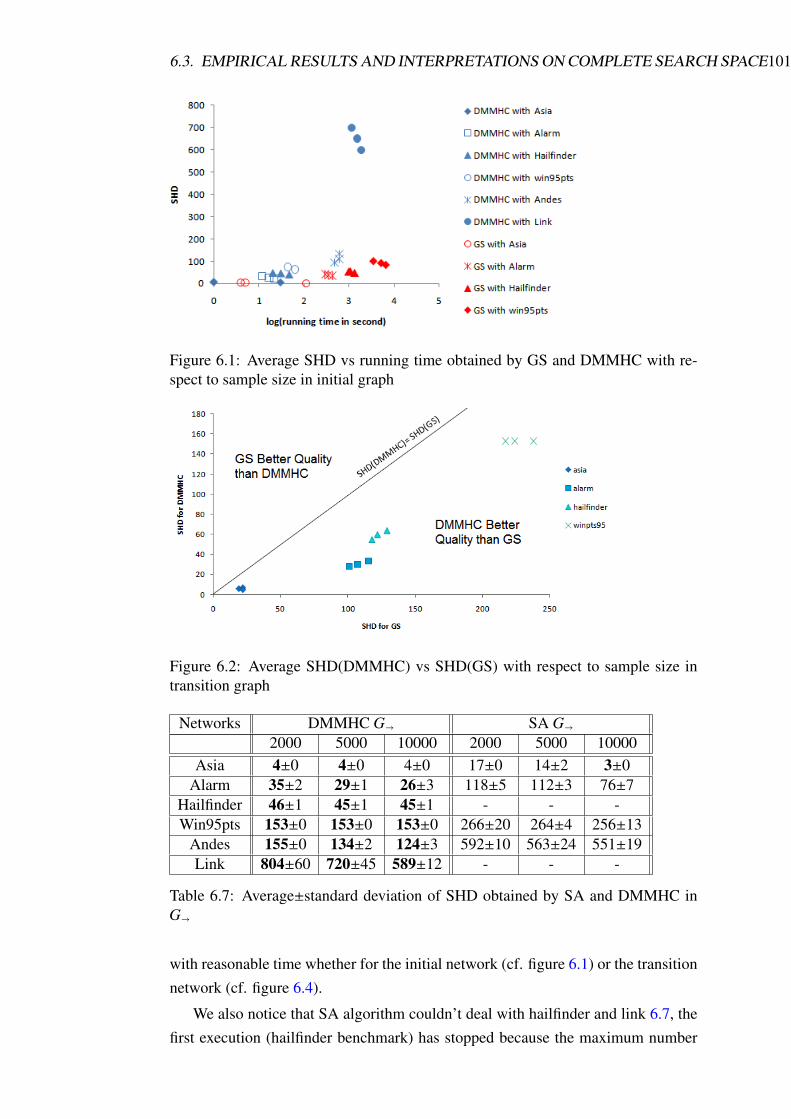
6.3. EMPIRICAL RESULTS AND INTERPRETATIONS ON COMPLETE SEARCH SPACE101
Figure 6.1: Average SHD vs running time obtained by GS and DMMHC with re-
spect to sample size in initial graph
Figure 6.2: Average SHD(DMMHC) vs SHD(GS) with respect to sample size in
transition graph
Networks DMMHC G� SA G�
2000 5000 10000 2000 5000 10000
Asia 4±0 4±0 4±0 17±0 14±2 3±0
Alarm 35±2 29±1 26±3 118±5 112±3 76±7
Hailfinder 46±1 45±1 45±1 - - -
Win95pts 153±0 153±0 153±0 266±20 264±4 256±13
Andes 155±0 134±2 124±3 592±10 563±24 551±19
Link 804±60 720±45 589±12 - - -
Table 6.7: Average±standard deviation of SHD obtained by SA and DMMHC in
G�
with reasonable time whether for the initial network (cf. figure 6.1) or the transition
network (cf. figure 6.4).
We also notice that SA algorithm couldn’t deal with hailfinder and link 6.7, the
first execution (hailfinder benchmark) has stopped because the maximum number
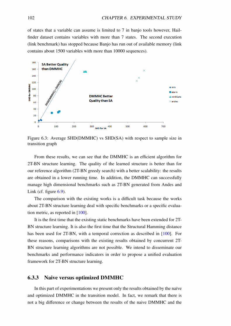
102 CHAPTER 6. EXPERIMENTAL STUDY
of states that a variable can assume is limited to 7 in banjo tools however, Hail-
finder dataset contains variables with more than 7 states. The second execution
(link benchmark) has stopped because Banjo has run out of available memory (link
contains about 1500 variables with more than 10000 sequences).
Figure 6.3: Average SHD(DMMHC) vs SHD(SA) with respect to sample size in
transition graph
From these results, we can see that the DMMHC is an efficient algorithm for
2T-BN structure learning. The quality of the learned structure is better than for
our reference algorithm (2T-BN greedy search) with a better scalability: the results
are obtained in a lower running time. In addition, the DMMHC can successfully
manage high dimensional benchmarks such as 2T-BN generated from Andes and
Link (cf. figure 6.9).
The comparison with the existing works is a difficult task because the works
about 2T-BN structure learning deal with specific benchmarks or a specific evalua-
tion metric, as reported in [100].
It is the first time that the existing static benchmarks have been extended for 2T-
BN structure learning. It is also the first time that the Structural Hamming distance
has been used for 2T-BN, with a temporal correction as described in [100]. For
these reasons, comparisons with the existing results obtained by concurrent 2T-
BN structure learning algorithms are not possible. We intend to disseminate our
benchmarks and performance indicators in order to propose a unified evaluation
framework for 2T-BN structure learning.
6.3.3 Naive versus optimized DMMHC
In this part of experimentations we present only the results obtained by the naıve
and optimized DMMHC in the transition model. In fact, we remark that there is
not a big difference or change between the results of the naive DMMHC and the
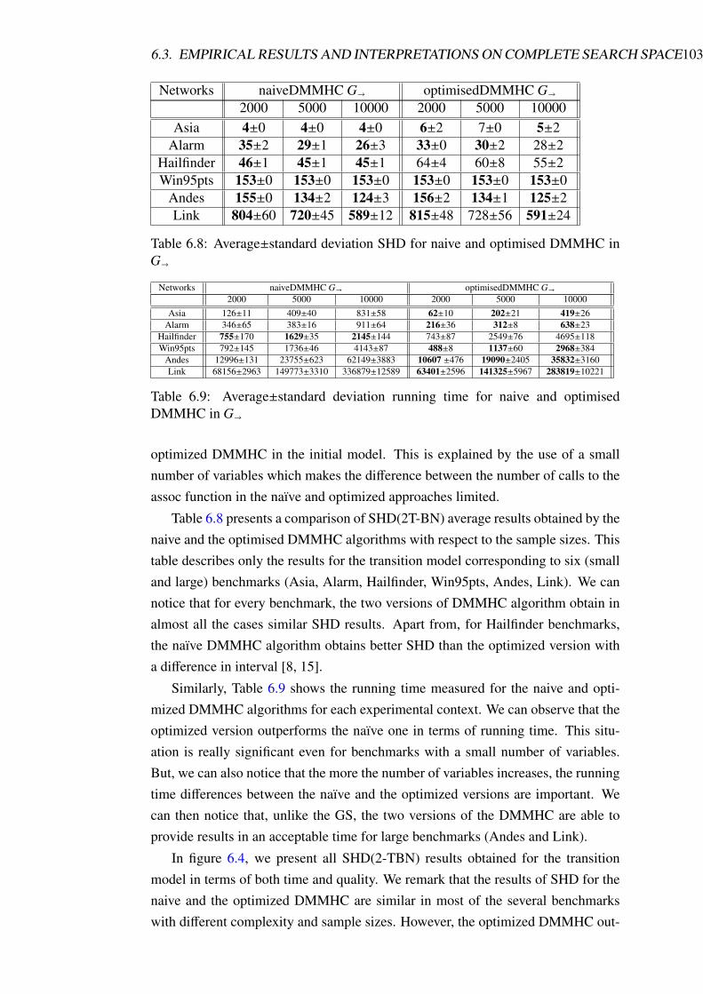
6.3. EMPIRICAL RESULTS AND INTERPRETATIONS ON COMPLETE SEARCH SPACE103
Networks naiveDMMHC G� optimisedDMMHC G�
2000 5000 10000 2000 5000 10000
Asia 4±0 4±0 4±0 6±2 7±0 5±2
Alarm 35±2 29±1 26±3 33±0 30±2 28±2
Hailfinder 46±1 45±1 45±1 64±4 60±8 55±2
Win95pts 153±0 153±0 153±0 153±0 153±0 153±0
Andes 155±0 134±2 124±3 156±2 134±1 125±2
Link 804±60 720±45 589±12 815±48 728±56 591±24
Table 6.8: Average±standard deviation SHD for naive and optimised DMMHC in
G�
Networks naiveDMMHC G� optimisedDMMHC G�
2000 5000 10000 2000 5000 10000
Asia 126±11 409±40 831±58 62±10 202±21 419±26
Alarm 346±65 383±16 911±64 216±36 312±8 638±23
Hailfinder 755±170 1629±35 2145±144 743±87 2549±76 4695±118
Win95pts 792±145 1736±46 4143±87 488±8 1137±60 2968±384
Andes 12996±131 23755±623 62149±3883 10607 ±476 19090±2405 35832±3160
Link 68156±2963 149773±3310 336879±12589 63401±2596 141325±5967 283819±10221
Table 6.9: Average±standard deviation running time for naive and optimised
DMMHC in G�
optimized DMMHC in the initial model. This is explained by the use of a small
number of variables which makes the difference between the number of calls to the
assoc function in the naıve and optimized approaches limited.
Table 6.8 presents a comparison of SHD(2T-BN) average results obtained by the
naive and the optimised DMMHC algorithms with respect to the sample sizes. This
table describes only the results for the transition model corresponding to six (small
and large) benchmarks (Asia, Alarm, Hailfinder, Win95pts, Andes, Link). We can
notice that for every benchmark, the two versions of DMMHC algorithm obtain in
almost all the cases similar SHD results. Apart from, for Hailfinder benchmarks,
the naıve DMMHC algorithm obtains better SHD than the optimized version with
a difference in interval [8, 15].
Similarly, Table 6.9 shows the running time measured for the naive and opti-
mized DMMHC algorithms for each experimental context. We can observe that the
optimized version outperforms the naıve one in terms of running time. This situ-
ation is really significant even for benchmarks with a small number of variables.
But, we can also notice that the more the number of variables increases, the running
time differences between the naıve and the optimized versions are important. We
can then notice that, unlike the GS, the two versions of the DMMHC are able to
provide results in an acceptable time for large benchmarks (Andes and Link).
In figure 6.4, we present all SHD(2-TBN) results obtained for the transition
model in terms of both time and quality. We remark that the results of SHD for the
naive and the optimized DMMHC are similar in most of the several benchmarks
with different complexity and sample sizes. However, the optimized DMMHC out-
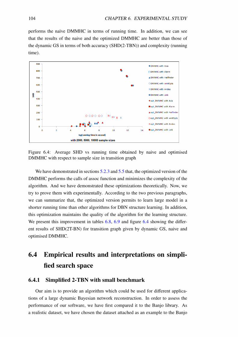
104 CHAPTER 6. EXPERIMENTAL STUDY
performs the naıve DMMHC in terms of running time. In addition, we can see
that the results of the naive and the optimized DMMHC are better than those of
the dynamic GS in terms of both accuracy (SHD(2-TBN)) and complexity (running
time).
Figure 6.4: Average SHD vs running time obtained by naive and optimised
DMMHC with respect to sample size in transition graph
We have demonstrated in sections 5.2.3 and 5.5 that, the optimized version of the
DMMHC performs the calls of assoc function and minimizes the complexity of the
algorithm. And we have demonstrated these optimizations theoretically. Now, we
try to prove them with experimentally. According to the two previous paragraphs,
we can summarize that, the optimized version permits to learn large model in a
shorter running time than other algorithms for DBN structure learning. In addition,
this optimization maintains the quality of the algorithm for the learning structure.
We present this improvement in tables 6.8, 6.9 and figure 6.4 showing the differ-
ent results of SHD(2T-BN) for transition graph given by dynamic GS, naive and
optimised DMMHC.
6.4 Empirical results and interpretations on simpli-
fied search space
6.4.1 Simplified 2-TBN with small benchmark
Our aim is to provide an algorithm which could be used for different applica-
tions of a large dynamic Bayesian network reconstruction. In order to assess the
performance of our software, we have first compared it to the Banjo library. As
a realistic dataset, we have chosen the dataset attached as an example to the Banjo
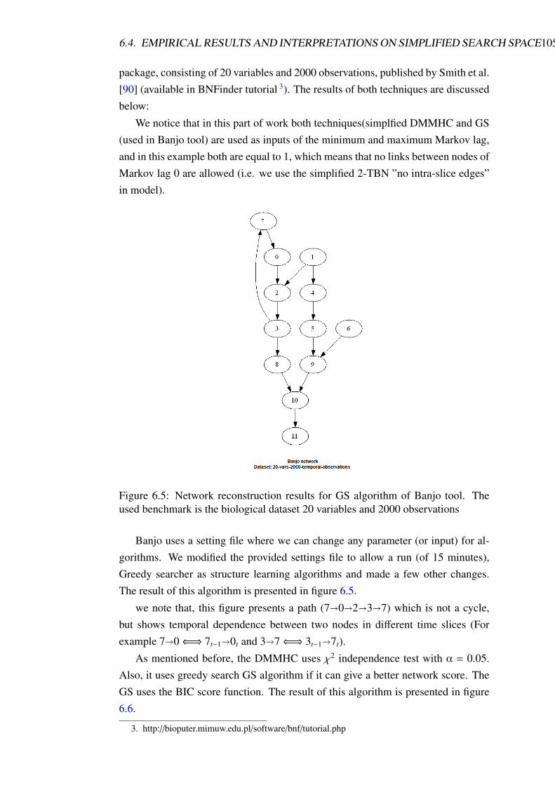
6.4. EMPIRICAL RESULTS AND INTERPRETATIONS ON SIMPLIFIED SEARCH SPACE105
package, consisting of 20 variables and 2000 observations, published by Smith et al.
[90] (available in BNFinder tutorial 3). The results of both techniques are discussed
below:
We notice that in this part of work both techniques(simplfied DMMHC and GS
(used in Banjo tool) are used as inputs of the minimum and maximum Markov lag,
and in this example both are equal to 1, which means that no links between nodes of
Markov lag 0 are allowed (i.e. we use the simplified 2-TBN ”no intra-slice edges”
in model).
Figure 6.5: Network reconstruction results for GS algorithm of Banjo tool. The
used benchmark is the biological dataset 20 variables and 2000 observations
Banjo uses a setting file where we can change any parameter (or input) for al-
gorithms. We modified the provided settings file to allow a run (of 15 minutes),
Greedy searcher as structure learning algorithms and made a few other changes.
The result of this algorithm is presented in figure 6.5.
we note that, this figure presents a path (7�0�2�3�7) which is not a cycle,
but shows temporal dependence between two nodes in different time slices (For
example 7�0⇐⇒ 7t−1�0t and 3�7⇐⇒ 3t−1�7t).
As mentioned before, the DMMHC uses χ2 independence test with α = 0.05.
Also, it uses greedy search GS algorithm if it can give a better network score. The
GS uses the BIC score function. The result of this algorithm is presented in figure
6.6.
3. http://bioputer.mimuw.edu.pl/software/bnf/tutorial.php
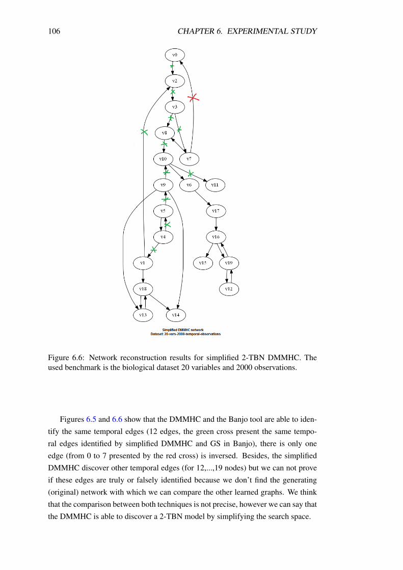
106 CHAPTER 6. EXPERIMENTAL STUDY
Figure 6.6: Network reconstruction results for simplified 2-TBN DMMHC. The
used benchmark is the biological dataset 20 variables and 2000 observations.
Figures 6.5 and 6.6 show that the DMMHC and the Banjo tool are able to iden-
tify the same temporal edges (12 edges, the green cross present the same tempo-
ral edges identified by simplified DMMHC and GS in Banjo), there is only one
edge (from 0 to 7 presented by the red cross) is inversed. Besides, the simplified
DMMHC discover other temporal edges (for 12,...,19 nodes) but we can not prove
if these edges are truly or falsely identified because we don’t find the generating
(original) network with which we can compare the other learned graphs. We think
that the comparison between both techniques is not precise, however we can say that
the DMMHC is able to discover a 2-TBN model by simplifying the search space.
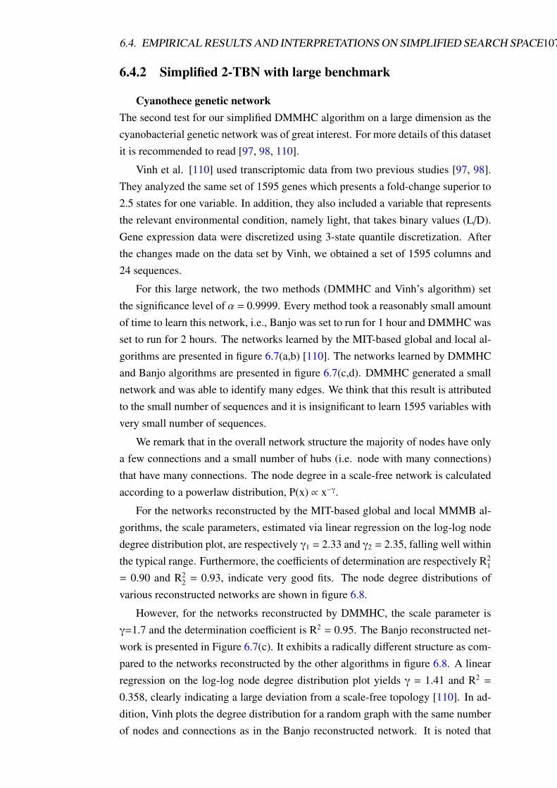
6.4. EMPIRICAL RESULTS AND INTERPRETATIONS ON SIMPLIFIED SEARCH SPACE107
6.4.2 Simplified 2-TBN with large benchmark
Cyanothece genetic network
The second test for our simplified DMMHC algorithm on a large dimension as the
cyanobacterial genetic network was of great interest. For more details of this dataset
it is recommended to read [97, 98, 110].
Vinh et al. [110] used transcriptomic data from two previous studies [97, 98].
They analyzed the same set of 1595 genes which presents a fold-change superior to
2.5 states for one variable. In addition, they also included a variable that represents
the relevant environmental condition, namely light, that takes binary values (L/D).
Gene expression data were discretized using 3-state quantile discretization. After
the changes made on the data set by Vinh, we obtained a set of 1595 columns and
24 sequences.
For this large network, the two methods (DMMHC and Vinh’s algorithm) set
the significance level of α = 0.9999. Every method took a reasonably small amount
of time to learn this network, i.e., Banjo was set to run for 1 hour and DMMHC was
set to run for 2 hours. The networks learned by the MIT-based global and local al-
gorithms are presented in figure 6.7(a,b) [110]. The networks learned by DMMHC
and Banjo algorithms are presented in figure 6.7(c,d). DMMHC generated a small
network and was able to identify many edges. We think that this result is attributed
to the small number of sequences and it is insignificant to learn 1595 variables with
very small number of sequences.
We remark that in the overall network structure the majority of nodes have only
a few connections and a small number of hubs (i.e. node with many connections)
that have many connections. The node degree in a scale-free network is calculated
according to a powerlaw distribution, P(x) ∝ x−γ.
For the networks reconstructed by the MIT-based global and local MMMB al-
gorithms, the scale parameters, estimated via linear regression on the log-log node
degree distribution plot, are respectively γ1 = 2.33 and γ2 = 2.35, falling well within
the typical range. Furthermore, the coefficients of determination are respectively R21
= 0.90 and R22= 0.93, indicate very good fits. The node degree distributions of
various reconstructed networks are shown in figure 6.8.
However, for the networks reconstructed by DMMHC, the scale parameter is
γ=1.7 and the determination coefficient is R2 = 0.95. The Banjo reconstructed net-
work is presented in Figure 6.7(c). It exhibits a radically different structure as com-
pared to the networks reconstructed by the other algorithms in figure 6.8. A linear
regression on the log-log node degree distribution plot yields γ = 1.41 and R2 =
0.358, clearly indicating a large deviation from a scale-free topology [110]. In ad-
dition, Vinh plots the degree distribution for a random graph with the same number
of nodes and connections as in the Banjo reconstructed network. It is noted that
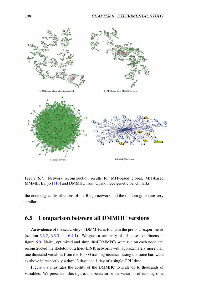
108 CHAPTER 6. EXPERIMENTAL STUDY
Figure 6.7: Network reconstruction results for MIT-based global, MIT-based
MMMB, Banjo [110] and DMMHC from Cyanothece genetic benchmarks
the node degree distributions of the Banjo network and the random graph are very
similar.
6.5 Comparison between all DMMHC versions
An evidence of the scalability of DMMHC is found in the previous experiments
(section 6.3.2, 6.3.3 and 6.4.1). We gave a summary of all these experimens in
figure 6.9. Naive, optimized and simplified DMMPCs were run on each node and
reconstructed the skeleton of a tiled-LINK networks with approximately more than
one thousand variables from the 10,000 training instances using the same hardware
as above in respectivly 4 days, 3 days and 1 day of a single-CPU time.
Figure 6.9 illustrates the ability of the DMMHC to scale up to thousands of
variables. We present in this figure, the behavior or the variation of running time
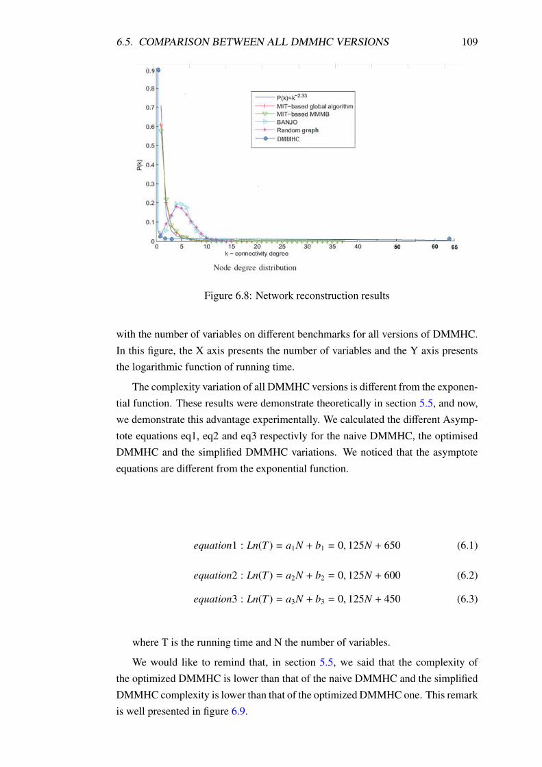
6.5. COMPARISON BETWEEN ALL DMMHC VERSIONS 109
Figure 6.8: Network reconstruction results
with the number of variables on different benchmarks for all versions of DMMHC.
In this figure, the X axis presents the number of variables and the Y axis presents
the logarithmic function of running time.
The complexity variation of all DMMHC versions is different from the exponen-
tial function. These results were demonstrate theoretically in section 5.5, and now,
we demonstrate this advantage experimentally. We calculated the different Asymp-
tote equations eq1, eq2 and eq3 respectivly for the naive DMMHC, the optimised
DMMHC and the simplified DMMHC variations. We noticed that the asymptote
equations are different from the exponential function.
equation1 : Ln(T ) = a1N + b1 = 0, 125N + 650 (6.1)
equation2 : Ln(T ) = a2N + b2 = 0, 125N + 600 (6.2)
equation3 : Ln(T ) = a3N + b3 = 0, 125N + 450 (6.3)
where T is the running time and N the number of variables.
We would like to remind that, in section 5.5, we said that the complexity of
the optimized DMMHC is lower than that of the naive DMMHC and the simplified
DMMHC complexity is lower than that of the optimized DMMHC one. This remark
is well presented in figure 6.9.

110 CHAPTER 6. EXPERIMENTAL STUDY
Figure 6.9: Complexity of all DMMHC versions
6.6 Conclusion
The experimental results, provided in this chapter, show that the proposed DMMHC
algorithms achieve a better performance than the other existing structure learning
for DBN such as Greedy Search or the Simulated Annuling algorithms.
The proposed approach was tested through real and standard benchmarks cre-
ated by our evaluation techniques for a dynamic case. Also, we validated the
DMMHC on a real biology field (Cyanothece genetic network). Nevertheless, the
main problem is that there is no commonly accepted benchmark that can be used to
learn with a large number of instances (i.e. Cyanothece genetic benchmark contains
only 24 instances) that can lead to more rigorous results.

7Conclusion
Sommaire
7.1 Summary . . . . . . . . . . . . . . . . . . . . . . . . . . . . . 112
7.2 Applications . . . . . . . . . . . . . . . . . . . . . . . . . . . 113
7.3 Limitations . . . . . . . . . . . . . . . . . . . . . . . . . . . . 114
7.4 Issues for future researches . . . . . . . . . . . . . . . . . . . 115
111
112 CHAPTER 7. CONCLUSION
7.1 Summary
In the different sections of this thesis work, we discussed in (the chapter 2 and
chapter 3), the problem of representation the Probabilistic graphical Models (PGM),
especially in the Bayesian networks and their extension Dynamic BN.
In chapter 2, we present the key concepts of Bayesian networks, structure learn-
ing methods of these models and all techniques used to evaluate these learning al-
gorithms. We concluded in this chapter that the hybrid method for learning the BN
performed better than the techniques based on constraints or those based on score.
We also noted that most of the studies use the methods based on the score for evalu-
ation, although this kind of method has disadvantages when the data size is reduced
and the calculation is costly when the number of variables is important.
In the same way, in chapter 3, we present the key concepts of the dynamic
bayesian network and the different structure learning studies of these models. We
also addressed to a discussion of the different elaborated works to evaluate their
DBN structure learning algorithms.
For these approaches, there are many weaknesses as they use their oun evalua-
tion Benchmarks and techniques to evaluate. In addition, we don’t find any online
availbale structure learning algorithm software for DBN, that can be compared to
our methods. The important conclusions that can be drawn from this study is that
the most of the studies use networks with small number of variables and score based
techniques for evaluation. This makes the comparison between our study and other
works more difficult.
In the chapters 4 and 5, we tried to solve the problems mentioned in the pre-
vious chapters. In chapter 4, we focused on solving the problem of evaluation for
the temporal graphical model as the DBN and especially the 2T-BN models. We
also introduced, tow contributions: the first is a large 2-TBN generation algorithm
inspired from the Tiling technique; the second is a novel metric to evaluate the per-
formance of DBN structure learning algorithms. It is inspired from the Structural
Hamming distance used in the static case, but it takes into account temporal back-
ground information.
In chapter 5, we developed a novel approach for DBN structure learning named
DMMHC. It is a hybrid method that uses a local search algorithm dealing with local
structure identification (DMMPC) and global model optimization constrained with
the local information (DMMHC). We demonstrated that this approach can easily
take into account the temporal dimension in order to provide some additional in-
formation about temporality that can then be used with a greedy search in order to
learn the global structure the initial model G0 and the transition one G�. As far as
we know, no method able to learn dynamic network models with such approaches
has been proposed previously.
7.2. APPLICATIONS 113
To analyze and validate the merits of our proposed and used methods, we car-
ried out some experiments, detailed in chapter 6, on standard large benchmarks
constructed with our method described in chapter 4. These benchmarks are derived
from the standard benchmarks used in the evaluation of structure learning methods
in a static case as Asia, alarm, hailfinder ...
The results have shown the significance of our novel algorithms for dynamic
Bayesian network structure learning on the level of scalability, complexity, running
time and accuracy (quality of construction models).
7.2 Applications
Since the sixties, saving the multi-dimensional and temporal data has increased
in many fields. ”Time” is an important concept in medical care [79, 89]. Several
studies done in the medical field for the evaluation of the nosocomial infections
(IN) predominance and the factors associated to its presence [37, 40]. In our future
studies, we are interested in solving this problem through the prediction of the prog-
nostic patient’s cases. Our system, named Decision Support System Nosocomial
Infection (DSS-NI), enables to predict their cases relying on the patient’s history
and medical treatment during his hospital stay. This work is important since physi-
ciens complain about incomplete and irregular data structure, which makes their job
more difficult. As a result, the predictions are judged to be poor in question of the
extracted knowledge [55, 60, 66, 99].
Nosocomial infections (NIs) continue to be a major problem. It causes high mor-
bidity and mortality. Consequently, it increases the length of hospitalization and the
cost of treatment. The supervision of NIs is an essential part of the infection con-
trol program. Therefore, prevention is better than cure for our patients. Successful
infection control measures depend on education at the level of healthcare workers
(HCWs), surveillance of the prevalent microorganisms and their antimicrobial re-
sistance patterns, and an efficient interdisciplinary collaboration. The supervision
activities are part of infection control efforts to improve the quality of hospital care.
Most of the research on the controls of the NI concentrate on the acquisition of this
supervision. Since a hospitalization may end up with the patient’s death.
In the decision support analysis initialized by Morton and Keen [88, 53], most of
the studies used in this domain are limited to the static aspect as the static Bayesian
Networks [4, 68]. This is insufficient for a dynamic decision making as in the
medical field. The dynamic processes which advance over time, known as Markov
decision processes, are used as the basis for prediction models. The techniques
such as decision-trees [71], neural networks [116], association rule, Hidden Makov
models [28, 46] and (dynamic) Bayesian networks [10, 32, 66, 79], developed by the
114 CHAPTER 7. CONCLUSION
artificial intelligence community, have become popular prediction models. Markov
models have been used in various medical applications. For instance, in medical
artificial intelligence (AI) Markov models often have a complex and multivariate
state representation. The models are represented as a dynamic Bayesian network
DBN [79], in this thesis we justify our choice to use this existing technique to
provide Markov models with multivariate and complex state descriptions of medical
data. Our objective is to extract models that can identify temporal patterns, predict
the daily prognostic of the patient’s state and test clinical hypotheses. Furthermore,
our models should be able to detect the future probable presence of a nosocomial
infection at ICU for tow levels 1) the processes regarding the eventual outcome of
ICU (to die or to survive), 2) and the processes related to the development of the
patient’s state (acquisition of NI) during of his/her hospitalization period.
The results of this thesis are relevant to these processes and demonstrate the in-
duction, inference, evaluation, and use of these models in practice data concerning
patients admitted to the ICU of Habib Bourguiba hospital (Sfax, Tunisia). The In-
tensive Care Unit of the CHU Habib Bourguiba of Sfax contains 22 beds in 11 boxes
of 2 beds. Each box is thus made up of 2 beds separated by a care zone containing
all that a nurse needs (compress, gloves, serum, drugs, etc.) to deal with his/her 2
patients. A nurse is responsible for the care of 2 patients. The majority of the pa-
tients admitted in ICU are known as ”heavy” because they require a 24h/24h care.
They are often connected to machines (artificial respirator, electrocardiogram, elec-
tric syringe, etc.) and/or connected to catheters (venous catheters, urinary probe,
thoracic drain...). These patients are often in a very delicate health situation. They
are vulnerable to new germs entering their bodies. For each appearance of infection
either nosocomial or not, it is necessary to send a blood sample to the laboratory
to carry out a antibiogram. According to the antibiogram result, an antibiotherapie
is prescribed. The problem of the antibiotherapie is that a germ can be sensitive to
the antibiotic during the first period and resisting a few weeks or months later. This
sensitivity can be different from an individual to another [64].
7.3 Limitations
Despite our multiple attempts to take into account all interactions that can occur
between the DBN structure learning and evaluation techniques, we still face a few
difficulties to justify the performance of our techniques. In our experiments we
compared our algorithms to only the GS and the SA algorithms. This is not enough
to show the utility of our approach applied on large benchmarks.
As a second limitation, we should point out that the DBN and more generally
BN also led to create a decision extension called influence diagrams (ID) [54] that
7.4. ISSUES FOR FUTURE RESEARCHES 115
can solve the decision problems. It is possible to distinguish the variables on which
it is possible to act, with respect to other contextual variables. Thus we can act on
the costs of each decision or utility with respect to each context. In this thesis, we
don’t have enough time to achieve this final part of the study.
The third limitation, is that in our experiment we did not use real data. For
two raisons: (1) First we didn’t have enough time to make experiments using data
generated from standard benchmarks and data from a real dataset. (2) The medical
database provided by Habib Bouguiba hospital is not well prepared for use in exper-
iments due to the small base size (less than 1000 cases and less than 100 variables).
However, we need thousands of variables to apply our learning algorithms.
7.4 Issues for future researches
Our main immediate perspective is to introduce some local improvements on our
algorithm. Our framework offers several opportunities for future research. Among
this, we believe that all the theoretical properties and experimentation results should
be extended. We have identified several perspective ideas:
1. Our next step in this direction is the adaptation of the structural Hamming
distance in order to take into account any background knowledge (forbidden
edges, required ones, partial ordering, ...).
2. We think that the quality of the structure reconstruction can be improved dur-
ing the global optimization using a more evolved meta-heuristic such as a
Tabu search instead of a standard hill-climbing algorithm.
3. We plan to extend our dynamic approach with the use of others local identifi-
cation methods such as PCD algorithm [80] that can correct it under faithful-
ness assumption.
4. Develop the structure learning algorithm for duration graphical model (DGM)
relying on what we have reached in this thesis.
5. Extend our approach for learning the dynamic models to a decisional task
with the use of influence diagram (ID) and dynamic decision models (DDM).
6. Apply the algorithms developed before for a decision support task in the med-
ical field. Indeed, the currently developed system, for ICU Habib Bourguiba
hospital of Sfax, to predict the occurrence of nosocomial infections (NI) is
based on the dynamic bayesian network. This system gives only the scores
for predicting occurrence of IN without proposing any decision. Our major
goal is to develop a decision support system to fight against the NI in the ICU
of Habib Bourguiba Hospital of Sfax.

ABayesian Network and Parameter
learning
Here we are looking for estimating the probability distributions from available
data. The estimation of the probability distributions, parametric or not, is a vast
and complex subject. We describe here the most commonly used methods in the
Bayesian networks, as the data are complete, for more information, we advise to
read [51, 41].
A.1 From completed data
A.1.1 Statistical Learning
In the case where all variables are observed, the easiest and most used method is
the statistical estimate. It estimates the probability of an event by the frequency of
occurrence of the event in the database. This approach, called maximum likelihood
(ML). It is defined by:
P(Xi = xk|Pa(Xi) = x j) =Ni, j,k∑k(Ni, j,k)
(A.1)
Where Ni, j,k is the number of events in the data base, for which the variable Xi is in
the state xk and its parents are in the configuration x j .
117
118 APPENDIX A. BAYESIAN NETWORK AND PARAMETER LEARNING
A.1.2 Bayesian Learning
The Bayesian estimation follows a different principle. It consists in finding the
most likely parameter thetta as the data were observed using the a priori knowl-
edge over the parameters (e.g. maximum a posteriori (MAP) estimation). If we
assume that each P(Xi, j \ Pa(Xi)) follows a multinomial distribution, the conjugate
distribution follows a Dirichlet distribution with the parameters αi, j,k
θMAPi, j,k (Xi = xk|Pa(Xi) = x j) =
Ni, j,k + αi, j,k − 1∑k(Ni, j,k + αi, j,k − 1)
(A.2)
αi, j,k are the parameters of the Dirichlet distribution associated with the prior
probability P(Xi = xk \ Pa(Xi) = x j).
A.2 From incomplete data
A.2.1 Nature of the missing data and their treatment
The real-world data usually contains missing entries. We need to deal with
incomplete data sets that looks like the following (example A.1):
X1 X2 X3 X1 X2 X3
1 1 1 2 1 1
2 ? 1 ? 1 1
1 2 1 ? ? ?
where ? indicates missing values.
Figure A.1: Example of BN structure
To deal with the missing values, we need to make the follwing assumptions:
– MCAR (Missing Completely At Random): the actual value of X and the event
X-is-missing are independent on data.
– MAR (Missing At Random): the actual value of X and the event X-is-missing
are conditionally independent given other observed variables.
– NMAR (Not Missing At Random): the actual value of X and the event X-
is-missing are conditionally independent given other observed and missing
variables.
A.2. FROM INCOMPLETE DATA 119
The situations MCAR and MAR are the easiest to solve, because the observed data
contain all the information necessary to estimate the distribution of the missing data.
When the missing data are MCAR, the earliest and simplest approach is the
analysis of complete examples. This method tried to estimate the parameters from
completed data sets of all the examples fully observed in the observed data.
Many methods attempt to estimate the parameters of a model from data in MAR.
For example, we can cite the sequential updating [92], Gibbs sampling [36], and the
expectation maximization algorithm (EM) [58].
A.2.2 EM algorithm
One algorithm for parameters learning from incomplete data: The expectation-
maximization (EM) algorithm. Developed in the Statistics community (Dempster
et al. 1977)[24]. Adapted for Bayesian networks by Lauritzen (1994) [58].
It is an iterative algorithm.
– Starts with an initial estimation θ0.
– At each iteration t:
– Expectation: Complete the data set based on θt.
– Maximization: Re-estimate parameters using the completed data set, ob-
taining θt+1.

BBenchmarking the dynamic bayesian
network
B.1 BNtiling for 2-TBN implementation
Our approach is based on five steps: (1) generating a standard BN; (2) tiling the
BN; (3) conversting the BN to DBN with the determined number of time slices; (4)
constructing the initial and transition models of DBN; (5) generating of data for the
new DBN; the benchmarking for 2T-BN process is described as follows:
1. Building a Bayesian network with HUGIN format (.net)
2. Generating data file from the network with .dat format used the geniesmile
tools.
3. Converting the generated data on matlab format and save them in a data file
(.mat)
data=data converter hugin(’../Data/network.dat’, ’../Data/ network.net’);
4. Use the ”bn tiling” process to generate the new network R1 with N copies of
the original network
network filename=’../Data/network.net’;
dataset filename=’../Data/data.mat’;
nodes=bn tiling(network filename, dataset filename, nbr variables*N, 2);
121

122APPENDIX B. BENCHMARKING THE DYNAMIC BAYESIAN NETWORK
Remark: N represents the number of copies ”tile” in R1. This command does
not give R1 in HUGIN format, so we have to create a method that allows the
construction of the new network with new transformations.
data=data converter hugin(’../Data/ data.dat’, ’../Data/ network.net’);
5. Extract all the characteristics of R1 and nodes (name, parents, table of prob-
abilities)
6. Generate the Dynamic Bayesian network R2 from network R1.
– Building the DBN with K time slices:
Hugin DBN(nodes, N, K);
– Building the initial and transition model by :
Hugin Net(nodes,1); % the initial model
Hugin Net(nodes,2); % the transition model
7. Generate the new database from R2 dynamic network used the geniesmile
tools.
B.2 Generating large Dynamic Bayesian Networks
Algorithm 15 Generating large Dynamic Bayesian Networks
Require: DAG M, number of copies (n), number of time slices (k)
Ensure: Return initial and transition models (Mi0, Mi�), and DBN Bi with N time slices
1: Bi is empty graph
2: Generate Dataset D for M
3: Create a large Bayesian network Mi with n copies of M by tiling
4: Mi0=Mi
5: Generate Dataset Di for Mi
% add priori Knowledges (Temporal dependencies)
6: Create Mi� with 2 copies of Mi by tiling
7: 2-TBN model = (Mi0, Mi�)
8: for all i≥0 and i≤k do
9: add Mi� to Bi
10: end for
11: Return Bi

CDMMHC: Dynamic Max Min Hill
Climbing
C.1 Proofs of propositions used by DMMHC
C.1.1 Proof proposition 5.2.2:
Let Vi , Vi+1 et Vi−1 be the variable sets respectively of time slices i, i+1 and i-1.
Let Ne+ be the set of candidates parents/children of variable T ∈ Vi (noted Ne+ =
CPCi
∪CCi+1)
∪CPi−1).
1. ∀ X ∈ Vi� T
Let p a be path from T to X through the node m ∈ Vi+1 and k its child (k ∈
Vi+1)
Because of temporality, there is at least one V-structure in the path p and m is
its well (middle node), so p contains at least one convergence: X � m � T.
(a) If m <CCi+1 and k <CCi+1 then the path p is blocked by CCi+1⇒ Indp(X
;T | CCi+1)
(b) If m ∈ CCi+1 then the path p is active by CCi+1 and we have dep(X ;T |m)
but this dependance is indirect between X and T, so it will be removed in
Phase II (Backward) of our algorithm and hence⇒ Indp(X ;T | CCi+1)
(c) If m < CCi+1 and k ∈ CCi+1 then there is at least one V-structure in the
path p’ and k is its middle node X� k �T⇒ Indp(X ;T | CCi+1)
123
124 APPENDIX C. DMMHC: DYNAMIC MAX MIN HILL CLIMBING
Let p be a path from T to X through the node m ∈ Vi−1
(a) If m ∈ CPi−1 then, because of temporality, there is at least a divergence
in the path p, so the path p is blocked by CPi−1 ⇒ Indp(X ;T | CPi−1)
Hence ∀ X ∈ Vi�, Min(Z⊆CPi−1) Assoc(X ;T | Z) = 0
we conclude that ∀ Z ⊆ Vi+1 ⇒ Indp(X ;T | Z)⇒ Indp(X ;T | CCi+1))
Hence ∀ X ∈ Vi�, Min(Z⊆CCi+1) Assoc(X ;T | Z) = 0
Hence MaxX∈Vi�T Min(Z⊆Ne+)Assoc(X;T | Z)
=MaxX∈Vi�T Min(Z⊆CPCi
∪CCi+1
∪CPi−1)Assoc(X;T | Z)
=MaxX∈Vi�T {Min(Z⊆CPCi)Assoc(X;T | Z),Min(Z⊆CCi+1)Assoc(X;T | Z),Min(Z⊆CPi−1)Assoc(X;T
| Z) }
=MaxX∈Vi�T {Min(Z⊆CPCi)Assoc(X;T | Z), 0,0}
=MaxX∈Vi�T Min(Z⊆CPCi)Assoc(X;T | Z)
2. ∀ X ∈ Vi+1
Our model is the first Markov-order P(Xt | X1:t−1) = P(Xt | Xt−1)
Hence MaxX∈Vi�T Min(Z⊆Ne+)Assoc(X;T | Z)
=MaxX∈Vi�T Min(Z⊆CPCi
∪CCi+1
∪CPi−1)Assoc(X;T | Z)
=MaxX∈Vi�T Min(Z⊆CPCi
∪CCi+1)Assoc(X;T | Z)
3. ∀ X ∈ Vi−1
Let p be a path from X to T through tne node m ∈ Vi+1 and K its child (k ∈
Vi+1)
Because of temporality, there is at least one V-structure in the path p and m is
its well (middle node), so p contains at least one convergence: X � m � T.
(a) If m < CCi+1 et k < CCi+1 then the path p is blocked by CCi+1⇒ Indp(X
;T | CCi+1)
(b) If m ∈ CCi+1 then the path p is active by CCi+1 and we have dep(X ;T |m)
but this dependance is indirect between X and T, so it will be removed in
Phase II (Backward) of our algorithm and hence⇒ Indp(X ;T | CCi+1)
(c) If m < CCi+1 et k ∈ CCi+1 then there is at least one V-structure in the
path p’ and k is its middle node X� k �T⇒ Indp(X ;T | CCi+1)
We conclude that ∀ Z ⊆ Vi+1 we have Indp(X ;T | Z)⇒ Indp(X ;T | CCi+1))
Hence ∀ X ∈ Vi�, Min(Z⊆CCi+1) Assoc(X ;T | Z) = 0
Hence MaxX∈Vi−1�T Min(Z⊆Ne+)Assoc(X;T | Z)
=MaxX∈Vi−1Min(Z⊆CPCi
∪CCi+1
∪CPi−1)Assoc(X;T | Z)
=MaxX∈Vi−1{Min(Z⊆CPCi)Assoc(X;T | Z),Min(Z⊆CCi+1)Assoc(X;T | Z),Min(Z⊆CPi−1)Assoc(X;T
C.1. PROOFS OF PROPOSITIONS USED BY DMMHC 125
| Z) }
=MaxX∈Vi−1{Min(Z⊆CPCi)Assoc(X;T | Z), 0,Min(Z⊆CPi−1)Assoc(X;T | Z)}
=MaxX∈Vi−1Min(Z⊆CPCi
∪CPi−1)Assoc(X;T | Z)
C.1.2 Proof proposition 5.4.1:
As we know, in the Forward phase of DMMHC we need to calculate the assoc
function. Function Assoc(X; T|Z) is an estimate of the strength of association (de-
pendency) of X and T given Z. To identify all X in CPt−1(T), we need to compute
the Assoc(X; T|CPt−1
∪CPCt) (see algorithm 12).
– in this case we don’t have CPCt(T) candidates. So, we mustn’t find any false
positives depending on the structure Assoc(X; T|CPt−1
∪CPCt)= Assoc(X;
T|CPt−1) .
– we mustn’t find any intra-connectivity in t-1 time slice. So, Assoc(X; T|CPt−1∪CPCt)= Assoc(X; T|∅) where X ∈ Vt−1 and Vt−1 is the set of all variables
in t-1 time slice.
maxX∈Vt−1
min Assoc(X; T |Z) = maxX∈Vt−1
minS⊆Z
Assoc(X; T |S ) (C.1)
= maxX∈Vt−1
minS⊆CP
∪CPC
Assoc(X; T |S ) (C.2)
= maxX∈Vt−1
minS⊆�
Assoc(X; T |S ) (C.3)
= maxX∈Vt−1
Assoc(X; T |∅) (C.4)

Bibliography
[1] Statlib repository. http://lib.stat.cmu.edu/;
http://www.liacc.up.pt/ ltorgo/Regression/stock.tgz. 58
[2] H. Akaike. Statistical predictor identification. Ann. Inst. Statist. Math.,
22:203–217, 1970. 37
[3] S. Andreassen, F.V. Jensen, S.K. Andersen, B. Falck, U. Kjærulff, M. Wold-
bye, A.R. Sørensen, A. Rosenfalck, and F. Jensen. MUNIN — an expert
EMG assistant. In Computer-Aided Electromyography and Expert Systems,
chapter 21. Elsevier Science Publishers, 1989. 45
[4] A. Antonucci and M. Zaffalon. Decision-theoretic specification of credal
networks: A unified language for uncertain modeling with sets of Bayesian
networks. International Journal of Approximate Reasoning, 49:345–361,
2008. 113
[5] Z. Aydin, A. Singh, J. Bilmes, and W.S Noble. Learning sparse models for
a dynamic Bayesian network classifier of protein secondary structure. BMC
Bioinformatics, 12:154, 2011. 56
[6] M. Bartlett and J. Cussens. Advances in Bayesian network learning using
integer programming. In Proceedings of the 29th Conference on Uncertainty
in Artificial Intelligence (UAI 2013). AUAI Press, 2013. 46
[7] T. Bayes. An essay towards solving a problem in the doctrine of chances.
Philosphical Transactions of the Royal Society, 53:370–418, 1763. 30
[8] I. Beinlich, G. Suermondt, R. Chavez, and G. Cooper. The alarm moni-
toring system: A case study with two probabilistic inference techniques for
belief networks. In Proceedings of the 2nd European Conference on AI and
Medicine, pages 247–256, Berlin, 1989. Springer-Verlag. 97
[9] C. Boutilier, R. Dearden, and M. Goldszmidt. Exploiting structure in pol-
icy construction. In Proceedings of the International Joint Conference on
Artificial Intelligence, pages 1104–1113, 1995. 58
[10] T. Charitos, Van der Gaag L.C, Visscher S., Schurink K.A.M., and Lucas
P.J.F. A dynamic Bayesian network for diagnosing ventilator-associated
pneumonia in icu patients. Expert Systems with Applications, 36:1249–1258,
2009. 113
127
128 BIBLIOGRAPHY
[11] D. Chickering. Learning Bayesian networks is np-complete. In InD. Fisher
and H. Lenz (Eds.), Learning from data: Artificial intelligence and statistics
V. Springer-Verlag, 1996. 35, 36, 37, 66
[12] D. Chickering, D. Geiger, and D.E. Heckerman. Learning Bayesian networks
is NP-hard. Technical Report MSR-TR-94-17, Microsoft Research Technical
Report, 1994. 66
[13] D. Chickering, C. Meek, and D. Heckerman. Large-sample learning of
Bayesian networks is np-hard. Journal of Machine Learning Research,
5:1287–1330, 2004. 66
[14] D.M. Chickering. Learning equivalence classes of Bayesian-network struc-
tures. Journal of Machine Learning Research, 2:445–498, 2002. 34
[15] C. Chow and C. Liu. Approximating discrete probability distributions with
dependence trees. IEEE Transactions on Information Theory, 14(3):462–
467, 1968. 37
[16] C. Conati, A. S. Gertner, K. VanLehn, and M. J. Druzdzel. On-line student
modeling for coached problem solving using Bayesian networks. In Pro-
ceedings of the Sixth International Conference on User Modeling (UM–96),
pages 231–242, 1997. 45, 97
[17] G. Cooper and E. Hersovits. A Bayesian method for the induction of proba-
bilistic networks from data. Maching Learning, 9:309–347, 1992. 37
[18] Chickering D. and Heckerman D. Efficient Approximation for the Marginal
Likelihood of Incomplete Data given a Bayesian Network. In UAI’96, pages
158–168. Morgan Kaufmann, 1996. 37
[19] Denver Dash and Marek Druzdzel. A robust independence test for constraint-
based learning of causal structure. In Proceedings of the Nineteenth Confer-
ence Annual Conference on Uncertainty in Artificial Intelligence (UAI-03),
pages 167–174, San Francisco, CA, 2003. Morgan Kaufmann. 98
[20] C.P. de Campos, Z. Zeng, and Q. Ji. Structure learning of Bayesian networks
using constraints. In Proceedings of the 26 th International Conference on
Machine Learning, Montreal, Canada, pages 113–120, 2009. 42
[21] Luis M. de Campos and Javier G. Castellano. Bayesian network learning al-
gorithms using structural restrictions. International Journal of Approximate
Reasoning, pages 233–254, 2007. 45
[22] M. de Jongh and M.J. Druzdzel. A comparison of structural distance mea-
sures for causal Bayesian network models. Recent Advances in Intelligent
Information Systems, Challenging Problems of Science, Computer Science
series, pages 443–456, 2009. 15, 46, 98, 99
BIBLIOGRAPHY 129
[23] T. Dean and K.A. Kanazawa. A model for reasoning about persistence and
causation. Artificial Intelligence, 93(2):1–27, 1989. 21, 50
[24] A. Dempster, N. Laird, and D. Rubin. Maximum likelihood from incompete
data via the em algorithm. Journal of the Royal Statistical Society, 39:1–38,
1977. 119
[25] T. Dietterich. Hierarchical reinforcement learning with the maxq value func-
tion decomposition. Journal of Artificial Intelligence Research, 13:227–303,
2000. 58
[26] T. G. Dietterich. Machine learning. In Nature Encyclopedia of Cognitive
Science, London: Macmillan, 2003. 20
[27] N. Dojer. Learning Bayesian networks does not have to be np-hard. In
Springer-Verlag Berlin Heidelberg, editor, MFCS 2006, LNCS 4162, pages
305–314, 2006. 53, 54, 56, 59, 60, 90
[28] R. Donat. Modelisation de la fiabilite et de la Maintenance a partir de
modeles Graphiques probabilistes. These de doctorat, INSA de Rouen,
France, 2009. 113
[29] A. S. FAST. Learning the structure of Bayesian networks with constraint
satisfaction. Phd, University of Massachusetts Amherst, 2010. 36, 44
[30] Y. Freund, H.S. Seung, E. Shamir, and N. Tishby. Selective sampling using
the query by committee algorithm. Machine Learning, 28:133–168, 1997.
41
[31] N. Friedman. The Bayesian structural em algorithm. In Proceedings of the
14th Conference on Uncertainty in Artificial Intelligence, pages 129–138,
San Francisco, 1996. Morgan Kaufmann. 55
[32] N. Friedman, K. Murphy, and S. Russell. Learning the structure of dynamic
probabilistic networks. In Gregory F. Cooper and Serafın Moral, editors,
Proceedings of the 14th Conference on Uncertainty in Artificial Intelligence
(UAI-98), pages 139–147, San Francisco, 1998. Morgan Kaufmann. 20, 55,
79, 86, 90, 113
[33] N. Friedman, I. Nachman, and D. Peer. Learning Bayesian network structure
from massive datasets: The ”sparse candidate” algorithm. In Proceeding
UAI’99 Proceedings of the Fifteenth conference on Uncertainty in artificial
intelligence, pages 206–215, 1999. 41
[34] Jose A. Gamez, Juan L. Mateo, and Jose M. Puerta. Learning Bayesian
networks by hill climbing: efficient methods based on progressive restriction
of the neighborhood. Data Mining and Knowledge Discovery, 22:106–148,
2011. 15, 98, 99
130 BIBLIOGRAPHY
[35] S. Gao, Q. Xiao, Q. Pan, and Q. Li. Learning dynamic Bayesian networks
structure based on Bayesian optimization algorithm. Advances in Neural
Networks, Computer Science, Springer Berlin / Heidelberg, 4492:424–431,
2007. 21, 55, 58, 59, 90
[36] S. Geman and D. Geman. Stochastic relaxation gibbs distributions, and the
Bayesian restoration of images. IEEE Transactions on Pattern Analysis and
Machine Intelligence, 6(6):721–741, 1984. 119
[37] M.F. Geyik, C. Ayaz, M.K. Celen, and C. USTUN. Surveillance of noso-
comial infections in dicle university hospital: a ten-year experience. Turk J
Med Sci, 38(6):587–593, 2008. 113
[38] M. Ghavamzadeh and S. Mahadevan. Continuous-time hierarchical rein-
forcement learning. In Proceedings of the International Conference on Ma-
chine Learning, pages 186–193, 2001. 58
[39] J.A. Gomez, J.L. Mateo, and J.M. Puerta. Learning Bayesian networks by
hill climbing: efficient methods based on progressive restriction of the neigh-
borhood. Data Mining and Knowledge Discovery, 22(1-2):106–148, 2011.
46
[40] Kallel H., Bouaziz M., Ksibi H., Chelly H., Hmida C.B., Chaari A., and
Rekik N. Prevalence of hospital-acquired infection in a tunisian hospital.
Journal of Hospital Infection, 59:343–347, 2005. 113
[41] D. Heckerman. A tutorial on learning with Bayesian network. In Michael I.
Jordan, editor, Learning in Graphical Models, pages 301–354, Boston, 1998.
117
[42] D. Heckerman, D. Geiger, and D. Chickering. Learning Bayesian networks:
The combination of knowledge and statistical data. Machine Learning,
20:197–243, 1995. 35, 37, 66
[43] J.W. Hwang, Y.S. Lee, and Cho S.B. Structure evolution of dynamic
Bayesian network for traffic accident detection. In IEEE Congress on Evolu-
tionary Computation, pages 1655–1671, 2011. 58, 60
[44] K. Hwang, B. Kim, and B. Zhang. Learning hierarchical Bayesian networks
for large-scale data analysis. In CONIP 2006, pages 670–679, 2006. 41
[45] Jaime S. Ide and Fabio G. Cozman. Random generation of Bayesian
networks. In Brazilian Symp. on Artificial Intelligence, pages 366–375.
Springer-Verlag, 2002. 45
[46] Georges J. and Luciano M. Prediction of financial time series with time-
line hidden Markov experts and anns. Wseas Transactions on Business and
Economics, 4(9):140–146, 2007. 113
BIBLIOGRAPHY 131
[47] Hulst J. Modeling physiological processes with dynamic Bayesian networks.
Technical report, Faculty of Electrical Engineering, Mathematics and Cop-
uter Science, 2006. 52
[48] C.S. Jensen and A. Kong. Blocking Gibbs sampling for linkage analysis in
large pedigrees with many loops. Research Report R-96-2048, Department
of Computer Science, Aalborg University, Denmark, 1996. 20
[49] C.S. Jensen and A. Kong. Blocking Gibbs sampling for linkage analysis in
large pedigrees with many loops. Research Report R-96-2048, Department
of Computer Science, Aalborg University, Denmark, 1996. 28, 45, 97
[50] A. Jonsson and A. Barto. Active learning of dynamic Bayesian networks in
Markov decision processes. Springer, SARA 2007,LNAI 4612, 19:273–284,
2007. 21, 58, 59
[51] M. Jordan. Learning in graphical models. In Academic Publishers, Dordecht,
The Netherlands, 1998. 117
[52] M.I. Jordan. Graphical models. Statistical Science (Special Issue on
Bayesian Statistics), 19:140–155, 2004. 20, 28
[53] P. Keen and M. Scott. An organizationnal perspective. Decision Support,
Systems Addison-Wesley Publishing Company, 1978. 113
[54] U.B. Kjærulff and A.L. Madsen. Bayesian Networks and Influence Dia-
grams. Springer Science+Business Media, LLC,, 2008. 114
[55] W.A. Knaus, D.P. Wagner, and J. Lynn. Short term mortality predictions for
critically ill hospitalised adults. Science and ethics., 254:389–394, 1991. 113
[56] k. Kojima, E. Perrier, S. Imoto, and S. Miyano. Optimal search on clus-
tered structural constraint for learning Bayesian network structure. Journal
of Machine Learning Research, 11:285–310, 2010. 46
[57] W. Lam and F. Bacchus. Using causal information and local measures to
learn bayesian networks. In Proceedings of the 9th Conference on Uncer-
tainty in Artificial Intelligence, pages 243–250. Morgan Kaufman Publishers,
1993. 37
[58] S. Lauritzen. The em algorithm for graphical association models with miss-
ing data. Computational Statistics and Data Analysis, 19:191–201, 1995.
119
[59] S. Lauritzen and D. Speigelhalter. Local computations with probabilities on
graphical structures and their application to expert systems. Royal statistical
Society B, 50:157–224, 1988. 17, 28, 68, 72, 73
[60] K.L. Lee, D.B. Pryor, F.E. Harrell, H.M. Califf, V.S. Behar, and W.L. Floyd.
Predicting outcome in coronary disease: statistical models vs. expert clini-
cians. Am J Med, 80(4):553–560, 1986. 113
132 BIBLIOGRAPHY
[61] P. Leray and O. Francois. Bnt structure learning package : Documentation
and experiments. Technical report, Laboratoire PSI - INSA Rouen, 2005. 58
[62] H. Lahdesmaki and I. Shmulevich. Learning the structure of dynamic
Bayesian networks from time series and steady state measurements. Mach
Learn, Springer Science and Business Media, 71(2-3):185–217, 2008. 54
[63] H. Ltifi, M. B. Ayed, G. Trabelsi, and A. M. Alimi. Using perspective wall
to visualize medical data in the intensive care unit. In Workshops at IEEE
International Conference on Data Mining ICDM2012, pages 72–78, 2012.
23
[64] H. Ltifi, G. Trabelsi, M. B. Ayed, and A. M Alimi. Dynamic decision support
system based on Bayesian networks -application to fight against the nosoco-
mial infections. International Journal of Advanced Research in Artificial
Intelligence, 1:22–29, 2012. 23, 114
[65] E. Maharaj. A pattern recognition of time series using wavelets. In 15th
Computational Statistics Conference of the International Association of Sta-
tistical Computing, Berlin, 2002. 58
[66] A.J. Marcel, G.T. Babs, and J.F. Peter. Dynamic Bayesian networks as prog-
nostic models for clinical patient management. Journal of Biomedical Infor-
matics, 41:515–529, 2008. 113
[67] D. Margaritis. Learning Bayesian networks model structure from data. Phd
thesis, Carnegie Mellon University,Pittsburgh, 2003. 37
[68] M.Correa, Bielza C., and Pamies-Teixeira J. Comparison of Bayesian net-
works and artificial neural networks for quality detection in a machining pro-
cess. Expert Systems with Applications, 36:7270–7279, 2009. 113
[69] Christopher Meek. Causal inference and causal explanation with background
knowledge. In Proceedings of the Eleventh Conference Annual Conference
on Uncertainty in Artificial Intelligence (UAI-95), pages 403–410. Morgan
Kaufmann, 1995. 17, 33, 34, 35
[70] M. Ben Messaoud. SemCaDo: an approach for serendipitous causal discov-
ery and ontology evolution. These de doctorat, University of Nantes, 2012.
17, 34
[71] E.M. Mugambi, A. Hunter, G. Oatley, and L. Kennedy. Polynomial-fuzzy
decision tree structures for classifying medical data. Knowledge-Based Sys-
tems, 17:81–87, 2004. 113
[72] K.P. Murphy. Bayes net toolbox, technical report. Technical report, MIT
Artificial Intelligence Laboratory, 2002. 98
[73] K.P. Murphy. Dynamic Bayesian Networks: Representation, Inference and
Learning. Phd, University of California, Berkeley, 2002. 21, 47, 50, 55, 66
BIBLIOGRAPHY 133
[74] K.P Murphy. Software packages for graphical models, Bayesian networks.
In Bull.Int.Soc.Bayesian Anal, page 14, 2007. 98
[75] R.E. Neapolitan. Learning Bayesian Networks. Pearson Education, 2004.
11, 27, 28, 32, 33, 35
[76] H.T. Nguyen. Reseaux bayesiens et apprentissage ensembliste pour l’etude
differentielle de reseaux de regulation genetique. These de doctorat, Univer-
site Nantes, 2012. 43
[77] Spirtes P., Glymour C., and Scheines R. Causation, prediction, and search.
Springer-Verlag, 1993. 33, 35, 37
[78] J. Pearl. Probabilistic Reasoning in Intelligent Systems: Networks of Plau-
sible Inference. Morgan Kaufmann Publishers, 1988. 20, 28, 32, 33, 37,
66
[79] L. Peelen, N.F. De Keizer, E. De Jonge, R.J. Bosman, A. Abu-Hanna, and
N. Peek. Using hierarchical dynamic Bayesian networks to investigate dy-
namics of organ failure in the intensive care unit. journal of Biomedical
Informatics, 43(2):273–286, 2010. 113, 114
[80] J.M. Pena, J. Bjorkegren, and J. Tegner. Scalable, efficient and correct learn-
ing of Markov boundaries under the faithfulness assumption. In Symbolic
and Quantitative Approaches to Reasoning with Uncertainty, volume 3571,
pages 136–147. Springer Berlin Heidelberg, 2005. 115
[81] M.J. Pena, J. Bjorkegren, and J. Tegner. Learning dynamic Bayesian net-
work models via cross-validation. Pattern Recognition Letters, 26:2295–
2308, 2005. 56, 58
[82] J.C. Rajapakse and J. Zhou. Learning effective brain connectivity with dy-
namic Bayesian networks. NeuroImage, 37:749–760, 2007. 56, 58, 59
[83] Ramsey, S.A. and Klemm, S.L. and Zak, D.E. and Kennedy, Kathleen A. and
Thorsson, Vesteinn and Li, Bin and Gilchrist, Mark and Gold, E.S. and John-
son, C.D. and Litvak, V. and Navarro, G. and Roach, J.C. and Rosenberger,
Carrie M. and Rust, A.G. and Yudkovsky, N. and Aderem, A. and Shmule-
vich, I. Uncovering a macrophage transcriptional program by integrating
evidence from motif scanning and expression dynamics. PLoS Comput Biol,
4(3):e1000021, 2008. 54
[84] J.W Robinson and A.J Hartemink. Learning non-stationary dynamic
Bayesian networks. Journal of Machine Learning Research, 11:3647–3680,
2010. 54, 57
[85] S. Rodrigues de Morais and A. Aussem. A novel scalable and data efficient
feature subset selection algorithm. In Proceedings of the European confer-
ence on Machine Learning and Knowledge Discovery in Databases - Part
134 BIBLIOGRAPHY
II, ECML PKDD ’08, pages 298–312, Berlin, Heidelberg, 2008. Springer-
Verlag. 39
[86] Kullback S. and Leibler R.A. On information and sufficiency. Annals of
Mathematical Statistics, 22(1):79–86, 1951. 43
[87] G. Schwartz. Estimating the dimension of a model. Annals of Statistics,
6:461–464, 1978. 37
[88] M. Scott. Computer based support for decision making. In Management
decision systems, Harvard University, Boston, MA, USA, 1971. 113
[89] Y. Shahar. Dimensions of time in illness: an objective view. Ann Interrn
Med, 132:45–53, 2000. 113
[90] V.A. Smith, j. Yu, T.V. Smulders, A.J. Hartemink, and E.D. Jarvis. Compu-
tational inference of neural information flow networks. PLoS Comput Biol,
2(11):e161, 2006. 59, 105
[91] Le Song, Mladen Kolar, and Eric P. Xing. Time-varying dynamic Bayesian
networks. 54, 58, 60
[92] D. Spiegelhalter and S. Lauritzen. Sequential updating of conditional proba-
bilities on directed graphical structures. Networks, 20:579–605, 1990. 119
[93] P. Spirtes. Conditional independence in directed cyclic graphical models
for feedback, technical report cmu-phil-54. Technical report, Department of
Philosophy, Carnegie Mellon University, Pittsburgh, 1994. 33
[94] N. Srebro. Maximum likelihood bounded tree-width Markov networks. In
Artificial Intelligence, pages 504–511, 2001. 38
[95] A. R. Statnikov, I. Tsamardinos, and C.F. Aliferis. An algorithm for genera-
tion of large Bayesian networks. Technical Report Technical Report DSL-03-
01, Department of Biomedical Informatics, Discovery Systems Laboratory,
Vanderbilt University, 2003. 46, 75
[96] H. Steck and T. S. Jaakkola. Unsupervised active learning in large domains.
In Proceedings of the Eighteenth Conference on Uncertainty in Artificial In-
telligence (UAI-02), pages 469–476, 2002. 41
[97] J. Stockel, E.A. Welsh, M. Liberton, Kunnvakkam, R. Aurora, and H.B.
Pakrasi. Global transcriptomic analysis of cyanothece 51142 reveals robust
diurnal oscillation of central metabolic processes. In Proceedings of the Na-
tional Academy of Sciences, volume 105, pages 6156–6161, 2008. 107
[98] J. Toepel, E. Welsh, T.C. Summerfield, H.B. Pakrasi, and L.A. Sherman. Dif-
ferential transcriptional analysis of the cyanobacterium cyanothece sp. strain
atcc 51142 during lightdark and continuous-light growth. Journal of Bacte-
riology, 190(11):3904–3913, 2008. 107
BIBLIOGRAPHY 135
[99] G. Trabelsi, M. Ben Ayed, and A.M. Alimi. Systeme d’extraction des con-
naissances a partir des donnees temporelles base sur les reseaux bayesiens
dynamiques. In RNTI E19 Extraction et Gestion des Connaissances EGC,
pages 241–246, Hammemet, Tunisie, JAN 2010. cepadues edition. 113
[100] G. Trabelsi, P. Leray, M. Ben Ayed, and A.M. Alimi. Benchmarking dy-
namic Bayesian network structure learning algorithms. In the 5th Interna-
tional Conference on Modeling, Simulation and Applied Optimization, pages
1–6, Hammemet, Tunisie, 2013. IEEExplorer. 2, 23, 71, 102
[101] G. Trabelsi, P. Leray, M. Ben Ayed, and A.M. Alimi. Dynamic MMHC :
a local search algorithm for dynamic Bayesian network structure learning.
In The Twelfth International Symposium on Intelligent Data Analysis (IDA
2013), pages 392–403. Springer LNCS, 2013. 2, 23
[102] I. Tsamardinos, C.F. Aliferis, and A.R. Statnikov. Time and sample efficient
discovery of Markov blankets and direct causal relations. In Proceedings of
ACM SIGKDD International Conference on Knowledge Discovery and Data
Mining, KDD, 36(4):673–678, 2003. 39, 42, 46
[103] I. Tsamardinos and G. Borboudakis. Permutation testing improves Bayesian
network learning. In European Conference on Machine Learning and Prin-
ciples and Practice of Knowledge Discovery in Databases (ECML-PKDD
2010), 2010. 96
[104] I. Tsamardinos, L. E. Brown, and C. F. Constantin, F. Aliferis. The max-min
hill-climbing Bayesian network structure learning algorithm. Mach. Learn.,
65(1):31–78, 2006. 33, 35, 37, 40, 42, 44, 45, 46, 66, 76, 79, 84, 88, 90
[105] I. Tsamardinos, F. Aliferis Constantin, and A.R. Statnikov. Algorithms for
large scale Markov blanket discovery. In 16th International FLAIRS Confer-
ence, pages 376–380, 2003. 39, 46
[106] I. Tsamardinos, A.R. Statnikov, L. E. Brown, and F. Aliferis Constantin.
Generating realistic large Bayesian networks by tiling. In Proceedings of
the 19th International Florida Artificial Intelligence Research Society Con-
ference (FLAIRS), pages 592–597, 2006. 69
[107] A. Tucker and X. Liu. Extending evolutionary programming methods to the
learning of dynamic Bayesian networks. In Proceedings of the Genetic and
Evolutionary Computation Conference, pages 923–929. Morgan Kaufmann,
1999. 90
[108] A. Tucker, X. Liu, and A. Ogden-Swift. Evolutionary learning of dynamic
probabilistic models with large time lags. International Journal of Intelligent
Systems, 16(5):621–646, 2001. 57, 90
136 BIBLIOGRAPHY
[109] T. Verma and J. Pearl. Equivalence and synthesis of causal models. In Pro-
ceedings of the Sixth Conference on Uncertainty in Artificial Intelligence,
pages 220–227, San Francisco, 1991. Morgan Kaufmann. 33, 34
[110] N.X. Vinh, M. Chetty, R. Coppel, and P. Wangikar. Local and global algo-
rithms for learning dynamic Bayesian networks. In IEEE 12th International
Conference on Data Mining (ICDM2012), pages 685–694, 2012. 17, 18, 52,
53, 54, 57, 59, 60, 61, 107, 108
[111] N.X Vinh, M. Chetty, R.L. Coppel, and P.P. Wangikar. Polynomial time algo-
rithm for learning globally optimal dynamic Bayesian network. In ICONIP
2011, Shanghai, China, volume 7064, pages 719–729. Springer, 2011. 56,
59, 60, 90
[112] H. Wang, K. Yu, and H. Yao. Learning dynamic Bayesian networks us-
ing evolutionary mcmc. In Proceedings of the International Conference on
Computational Intelligence and Security, pages 45–50, 2006. 56, 90
[113] K. Wang, J. Zhang, and F. Shen. Adaptive learning of dynamic Bayesian
networks with changing structures by detecting geometric structures of time
series. Knowl Inf Syst, 17:121–133, 2008. 21, 54, 57, 58
[114] B. Wilczynski and N. Dojer. Bnfinder: exact and efficient method for learning
Bayesian networks. bioinformatics, 25(2):286–287, 2009. 53, 56, 59, 60, 98
[115] M. Wynkoop and T. Dietterich. Learning mdp action models via discrete
mixture trees. Springer-Verlag Berlin Heidelberg, ECML PKDD, pages 597–
612, 2008. 57
[116] J. Xu, H. Ge, X. Zhou, J. Yan, Q. Chi, and Z. Zhang. Prediction of vascular
tissue engineering results with artificial neural networks. journal of Biomed-
ical Informatics, 38:pp417–421, 2005. 113

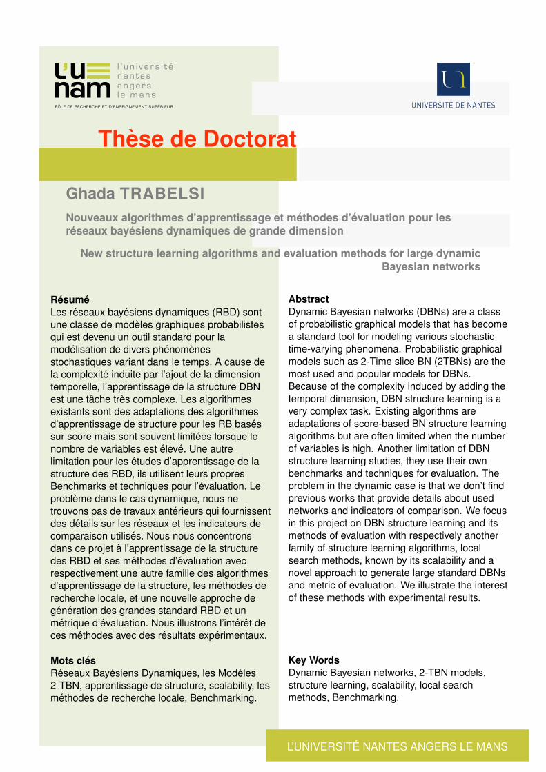
These de Doctorat
Ghada TRABELSI
Nouveaux algorithmes d’apprentissage et methodes d’evaluation pour lesreseaux bayesiens dynamiques de grande dimension
New structure learning algorithms and evaluation methods for large dynamicBayesian networks
Resume
Les reseaux bayesiens dynamiques (RBD) sont
une classe de modeles graphiques probabilistes
qui est devenu un outil standard pour la
modelisation de divers phenomenes
stochastiques variant dans le temps. A cause de
la complexite induite par l’ajout de la dimension
temporelle, l’apprentissage de la structure DBN
est une tache tres complexe. Les algorithmes
existants sont des adaptations des algorithmes
d’apprentissage de structure pour les RB bases
sur score mais sont souvent limitees lorsque le
nombre de variables est eleve. Une autre
limitation pour les etudes d’apprentissage de la
structure des RBD, ils utilisent leurs propres
Benchmarks et techniques pour l’evaluation. Le
probleme dans le cas dynamique, nous ne
trouvons pas de travaux anterieurs qui fournissent
des details sur les reseaux et les indicateurs de
comparaison utilises. Nous nous concentrons
dans ce projet a l’apprentissage de la structure
des RBD et ses methodes d’evaluation avec
respectivement une autre famille des algorithmes
d’apprentissage de la structure, les methodes de
recherche locale, et une nouvelle approche de
generation des grandes standard RBD et un
metrique d’evaluation. Nous illustrons l’interet de
ces methodes avec des resultats experimentaux.
Abstract
Dynamic Bayesian networks (DBNs) are a class
of probabilistic graphical models that has become
a standard tool for modeling various stochastic
time-varying phenomena. Probabilistic graphical
models such as 2-Time slice BN (2TBNs) are the
most used and popular models for DBNs.
Because of the complexity induced by adding the
temporal dimension, DBN structure learning is a
very complex task. Existing algorithms are
adaptations of score-based BN structure learning
algorithms but are often limited when the number
of variables is high. Another limitation of DBN
structure learning studies, they use their own
benchmarks and techniques for evaluation. The
problem in the dynamic case is that we don’t find
previous works that provide details about used
networks and indicators of comparison. We focus
in this project on DBN structure learning and its
methods of evaluation with respectively another
family of structure learning algorithms, local
search methods, known by its scalability and a
novel approach to generate large standard DBNs
and metric of evaluation. We illustrate the interest
of these methods with experimental results.
Mots cles
Reseaux Bayesiens Dynamiques, les Modeles
2-TBN, apprentissage de structure, scalability, les
methodes de recherche locale, Benchmarking.
Key Words
Dynamic Bayesian networks, 2-TBN models,
structure learning, scalability, local search
methods, Benchmarking.
L’UNIVERSITE NANTES ANGERS LE MANS