News Shocks and Costly Technology Adoption�

Yi-Chan Tsaiy

November 10, 2009

Abstract

I study the macroeconomic response to news of future technological innovation un-

der the assumption that �rms cannot frictionlessly shift from existing capital stocks

to new varieties associated with the impending advance in technology. Combining

this new element with variable capital utilization and preferences designed to minimize

wealth e¤ects on labor supply, I develop a model that simultaneously accounts for four

stylized facts: (1) slow di¤usion of new technologies, (2) lumpiness in microeconomic

investment, (3) stock prices leading measured productivity, and (4) comovement of

consumption, investment and labor hours. On news of a coming technological innova-

tion, �rms begin to invest in new capital goods which will allow them to bene�t from

the innovation once it arrives. Because �xed costs lead some to delay adoption, there

is slow di¤usion of the new technology. At the �rm level, investment in new technology

follows an (S, s) rule, and at the aggregate level the model generates a hump-shaped

investment pattern typical of the data. Moreover, the introduction of new capital

causes the price of old capital to fall, leading stock prices to rise on news of the new

technology. Finally, variable capital utilization slows the onset of diminishing returns

to labor, so that work hours rise instantly, permitting rises in both consumption and

investment.

JEL E32, O33

Keywords: Endogenous Technology Adoption, Business Cycles, News Shocks

�I am indebted to Aubhik Khan, Julia Thomas and Bill Dupor for valuable advice and support, as wellas Paul Evans, Masao Ogaki, Nan Li, Belton Fleisher, Pok-Sang Lam, Yuko Imura, Tamon Takamura,Seungho Nan, Kerry Tan, Andreas Schick, and Michael Sinkey for helpful discussions. All errors are my ownresponsibility.

yDepartment of Economics, The Ohio State University, 410 Arps Hall, 1945 N. High Street, Columbus,OH 43210 Email address: tsai.181@osu.edu

1

1 Introduction

Macroeconomics has witnessed a revival of interest in expectations-driven business cycles in

recent years, motivated in part by the information-technology-related investment boom of

the 1990s. A body of empirical evidence has shown that, following a positive news shock,

households and �rms increase both consumption and investment in anticipation of future

technological innovation.1 Furthermore, if the anticipated technological improvement later

fails to meet expectations, consumption and investment will fall, generating a recession.

Because this type of boom-bust cycle can occur without technological regress, many have

argued that news about future productivity improvements may be an important source of

business cycle �uctuations.

Unfortunately, when researchers incorporate news shocks into standard dynamic stochas-

tic general equilibrium models, the resulting model predictions are at odds with both the

mechanisms and the empirical evidence outlined above. In particular, while consumption

increases in response to a positive news shock, investment is predicted to decrease. Thisproblem arises because labor, and thus output, does not rise in response to the shock, so any

rise in consumption must come at the expense of investment.

Recognizing the problem above, several recent papers have incorporated various mecha-

nisms into standard models to stimulate positive labor and investment responses to positive

news, and thus develop more successful models of boom-bust cycles. Leading examples

include Beaudry and Portier (2004), Christiano, Ilut, Motto, and Rostagno (2007) and

Jaimovich and Rebelo (2008). Each of these models succeeds in generating positive co-

movement between consumption and investment. However, each also assumes that capital

goods acquired at di¤erent times are perfect substitutes in production, despite empirical

evidence that capital productivity is speci�c to a particular technology. Furthermore, in

almost every existing model designed to reconcile the idea of boom-bust cycles with observed

business cycles, the assumption of convex investment adjustment costs plays a vital role in

stimulating coincident rises in labor, consumption and investment on the arrival of positive

news. Although convex adjustment costs may have desired e¤ects in the aggregate, they are

known to be inconsistent with microeconomic investment patterns.2

1Schmitt-Grohe and Uribe (2008) estimate the contribution of anticipated technology shocks to businesscycles in the postwar United States using a Bayesian method. They �nd that output, consumption, invest-ment and labor all increase in response to anticipated shocks, and these shocks explain more than two thirdsof aggregate �uctuations. Similarly, Beaudry and Portier (2006) show that consumption, investment andlabor hours all rise in response to an anticipated technology shock, as identi�ed by a vector error correctionmodel. Their study isolates anticipated shocks as the source of roughly one half of business cycle �uctuations.

2Because convex adjustment costs encourage �rms to smooth any single investment project over manyperiods, they rule out the large and occasional (or lumpy) investment activities observed in variousestablishment-level studies. Using U.S. manufacturing data, Doms and Dunne (1993) and Cooper, Halti-

2

I develop a general equilibrium vintage capital model wherein (a) technological progress

is capital-embodied and (b) �rms can replace capital of one vintage with capital of a newer

vintage only upon payment of �xed adoption costs. I treat a news shock as information

of a coming large technological innovation that will require costly technology adoption to

be useful.3 Following news of a technological leap, because such large advances are capital

embodied, �rms understand that they must purchase a new type of capital to realize any

productivity bene�t. More speci�cally, �rms cannot bene�t by simply purchasing more of

their existing variety of capital, but instead must acquire the capital designed for the new

technology. Next, I assume that �rms must pay �xed adoption costs in order to replace their

existing capital with new-vintage capital. Given idiosyncratic di¤erences in adoption costs,

this microeconomic friction leads to gradual technology adoption in the aggregate. Firms

encountering low adoption costs upgrade their capital immediately, while �rms facing higher

current costs delay adoption to a later date. As a result, a new technology di¤uses slowly,

and di¤erent vintages of capital can coexist for an extended time following news of a coming

technology advance. Moreover, at the �rm level, investment in new technology follows an

(S,s) rule, while the model generates a hump-shaped aggregate investment pattern typical

of the data, (see Christiano, Eichenbaum and Evans (2005)).

I combine the technology di¤usion mechanism described above with two elements rou-

tinely adopted in the news shock literature to encourage an immediate labor supply response

(variable capital utilization and preferences with minimal wealth e¤ects on labor supply)

and examine whether my resulting model of technology adoption generates the desired co-

movement between consumption, labor hours, and investment following a news shock. I

�nd that the model not only succeeds in this respect but also succeeds with regard to three

additional stylized facts commonly missed by news shock models: the slow di¤usion of new

technologies, the lumpiness in microeconomic investment, and the fact that stock prices lead

measured productivity.

One interesting feature of my model is the endogenous determination of the price of old

capital relative to that of new capital. Because only new capital can be used e¤ectively with

a new technology, old capital is not perfectly substitutable for new capital. As a result,

the resale price of old capital drops below the unit purchase price of new capital following a

wanger and Power (1999) document that lumpy investment episodes represent a large fraction of a typicalestablishment�s cumulative capital adjustment over time. Moreover, within a typical year, roughly one-quarter of aggregate investment arises from the activities of establishments exhibiting investment spikes.Most importantly, in terms of cyclical changes, these studies uncover a strong positive correlation betweenaggregate investment and the number of establishments exhibiting spikes.

3In the absence of a news shock, technology changes are small, ongoing improvements of the standardvariety. In such times, �rms frictionlessly adjust their capital stocks to o¤set the e¤ects of physical andeconomic depreciation.

3

positive news shock. This fall in the relative price of old capital implies a drop in replacement

costs, which leads stock prices to rise at the impact of the shock.

There is substantial evidence of capital embodied technological progress consistent with

the framework I adopt. Greenwood, Hercowitz, and Krusell (1997) report that an e¢ ciency

increase in capital due to improved technology can account for a substantial portion of output

growth in the postwar U.S. In particular, they argue that the decline in the relative price of

equipment in the postwar era, alongside the rising ratio of equipment to GDP, is evidence of

technological progress in equipment production.4 Bahk and Gort (1993) study micro-level

data on output and capital vintage from more than 2000 �rms across 41 industries and �nd

that a one year change in the average age of capital is associated with a 2.5%-3.5% change

in output.5 In addition, historical studies such as Devine (1983) document that, after the

Second Industrial Revolution, manufacturers found it necessary to build new �rms in order

to adopt new technology based on electricity. Similarly, David (1990) argues that �the slow

pace of (electricity) adoption prior to the 1920s was largely attributable to the unpro�tability

of replacing still serviceable manufacturing �rms embodying production technologies adapted

to the old regime of mechanical power derived from water and steam.�

Most technology adoption costs are nonconvex in nature and incurred only when a �rm

wishes to adjust its technology level. We list two such costs for example. One is capital

expenditure associated with technology adoption. The other is organization costs associated

with the accumulation of �rm-speci�c knowledge. Even after new capital is acquired, �rms

still need to learn how to apply the new technology. Since the nature of a new technology

di¤ers from the existing technology, its proper use and implementation may require a sub-

stantial reorganization of the production process. Schurr et. al. (1990) discuss the process

of learning following new applications of electricity to �rm and machine design. Similarly,

companies that adopted IT did not become more productive without also adopting certain

complementary changes in their business organization.

There is also ample evidence in favor of the pattern of technology adoption predicted by

my model. Studies such as David (1990) examine dynamic adjustments following technologi-

cal advances and document that new technology does not immediately accelerate productiv-

ity growth but rather di¤uses gradually. For example, in the Second Industrial Revolution,

the development of electricity did not immediately generate higher productivity; however,

4This interpretation also applies to the IT revolution, since substantial high-tech investment accompaniedthe declining relative price of IT over the past three decades.

5Campbell (1998) �nds that the entry rate covaries positively with output and total factor productivitygrowth, and the exit rate leads all three of these. He argues that a vintage capital model with technologicalprogress embodied in new plants is consistent with this evidence. Elsewhere, using measures of obsoles-cence, Boddy and Gort (1974) �nd that capital embodied technical change is an important component ofproductivity growth.

4

it was followed by a prolonged period of rapid productivity acceleration. Similarly, in the

case of the IT revolution, productivity began to accelerate roughly two decades after U.S.

businesses had invested in information technology.6 Atkeson and Kehoe (2001) argue that

this delay in productivity increase was caused by the slow di¤usion of new technologies as

well as the learning process required for �rms to e¤ectively use those technologies.

As mentioned above, my paper di¤ers from most studies in the news shock literature in

two important ways; it does not rely on convex adjustment costs to gradualize aggregate

investment, and it avoids the counterfactual assumption that all capital goods are equally

compatible with a new technology. The model most closely related to mine is that of Comin,

Gertler, and Santacreu (CGS, 2008), given its emphasis on endogenous technology di¤usion

following a news shock. Relative to that study, my model is distinguished along three

margins. First, CGS assume that any new technology is freely available to all �rms once

it is successfully adopted by one, and they emphasize the productivity gains arising from

the production of a wider variety of intermediate inputs in a monopolistically competitive

setting. By contrast, I consider a perfectly competitive environment wherein technology

adoption is a costly activity for every �rm; a �rm�s productivity rises with the arrival of a

new technology in my model only if that �rm has paid to acquire the new vintage of capital

compatible with the new technology. Second, I assume that, once a �rm pays its adoption

cost to purchase new capital, that �rm will be able to use the associated new technology with

certainty. CGS instead assume that the probability of successfully adopting a new variety of

intermediate goods is increasing in the level of �nal output devoted to technology adoption.

This assumption, alongside variable capital utilization, allows output to rise at the impact

of a news shock, which is critical in generating the rise in investment in their model. Finally,

while the CGS model succeeds in generating co-movement in consumption and investment

following a news shock, it delivers gradual rises in output and TFP consistent with the

evidence above only with the inclusion of several additional frictions (habit formation in

consumption, convex investment adjustment costs and Calvo price stickiness). My model

requires no such extension.

The remainder of this paper is organized as follows. In the next section, I develop

my general equilibrium model of news shocks with capital embodied technological progress

and costly technology adoption. In section 3, I specify the model�s functional forms and

parameter values. Section 4 displays the transitional dynamics in this economy following a

news shock and discusses how these dynamics arise, isolating the role played by each model

6This is sometimes refered to as the computer paradox based on Robert Solow�s observation duringthe 1970-1990 period that one could see evidence of the computer everywhere except in the productivitystatistics.

5

ingredient mentioned above. Finally, section 5 concludes.

2 General equilibriummodel with technology adoption

I study a general equilibrium vintage capital model embedded with a technology adoption

decision. There is new technology of which news arrives T1 periods in advance. During

times of abrupt technological transitions, like the IT Revolution, existing capital goods are

no longer perfect substitutes for new capital. Understanding this, �rms must decide when

to replace their existing capital with new capital. This adoption is not costless; it involves

the payment of �xed adoption costs. Given idiosyncratic di¤erences in these adoption costs,

both vintages of capital coexist, and new technologies di¤use slowly across �rms through

their adoption decisions. There are three economic agents in this economy: (1) households,

(2) �rms that have adopted the new technology, and (3) �rms that continue to use the

old technology. I describe their optimization problems below following a description of the

technological environment.

2.1 Capital-embodied technological process

In period 0, the economy is in an initial steady state and the capital-embodied technology

level equals "0. In the next period, news arrives that there will be a permanent technology

improvement associated with a new type of capital beginning in period T1. More speci�cally,

agents know that productivity will remain unchanged until the materialization of the new

technology and then exhibit a single discrete jump. They also know that each �rm must

purchase a new vintage of capital in order to bene�t from the advance in technology when

it arrives.

The new type of capital is compatible with both the new and the old technology, while the

old type of capital is compatible with only the old technology. Therefore, the productivity

of old capital does not change when the technological advance happens, i.e., "0;t = "0, 8t.By contrast, the productivity attached to the new capital rises with the arrival of the new

technology, as shown below.

"1;t =

("0 for t < T1,

"1 > "0 for t � T1(1)

6

2.2 Firms�optimization problems

I deviate from the standard assumption that capital is homogeneous and instead assume

that productivity varies across vintages of capital. I use the subscript i 2 f0; 1g to identifyvariables associated with each of the two capital vintages. Speci�cally, k0 and "0 represent

the per-�rm stock and the productivity associated with the old vintage of capital. Simi-

larly, k1 and "1 represent the per-�rm stock and the productivity of the new vintage. Each

�rm produces output using its predetermined capital stock, ki, labor hours, ni, and capital

utilization rates, hi, via a decreasing returns to scale production function, zf ("ihiki; ni).

Here, z re�ects stochastic total factor productivity which is common across �rms. I assume

that z follows a Markov chain z 2 fz1; :::; zNzg, where Pr(z0 = zjj z = zi)� �ij > 0, andPNzj=1 �ij = 1 for each i = 1; :::; Nz. Let s represent the distance between date t and the

time that news shocks is realized, i.e, s = maxfT1 � t; 0g. Firms take as given these twoexogenous components of the aggregate state, (z; s), as well as the endogenous component,

�, that represents the fraction of all �rms that have adopted the new technology.

At any point in time, each �rm is distinguished by its capital productivity, "i, its pre-

determined capital stock, ki, and its current idiosyncratic draw of a �xed cost associated

with technology adoption, � 2 [�L; �U ], which is denominated in units of labor. Given theaggregate state of the economy, each �rm chooses its current level of employment, its capital

utilization rate and its investment.

The investment decision involves a choice of whether to switch from the existing capital

(technology) to the new, more e¢ cient capital (technology) or to continue operating with the

existing capital. A �rm adopting the new capital must pay a one-time technology adoption

cost, �. This implies the forfeit of w(z; �; s)� units of current output, where w(z; �; s) denotes

the real wage rate. Note that these �xed costs do not apply to investment at any time other

than the single date in which the �rm �rst adopts the new capital. Therefore, if a �rm decides

to continue operating with its current vintage of capital, it undertakes frictionless capital

adjustment. The �rm�s capital stock evolves according to k0i = (1� �(hi)) ki + ii, where ii is

the current investment associated with vintage i and �(hi) is the capital depreciation rate. I

assume that depreciation is increasing and convex in the rate of capital utilization; �0(h) > 0

and �00(h) > 0.

A �rm can operate only one technology at a time. Consequently, every �rm in the

economy has only one vintage of capital at any date. For �rms that have previously adopted

the new technology, adoption costs are irrelevant, since I study a single discrete change in

technology. Those �rms choose employment, n1, a capital utilization rate, h1, and a capital

stock for the next period, k01, to maximize their expected discounted pro�ts. The value of

any such �rm is listed below, with the subscript 1 on the value function indicating that the

7

�rm has previously adopted the new capital.

v1 (k1; z; �; s) � maxn1;h1;k01

�zf ("1h1k1; n1)� w(z; �; s)n1 + (1� �(h1)) k1 (2)

�k01 +NzXj=1

dj (z; �; s) v1 (k01; zj; �

0; s0)�

Here, �rms discount their next-period expected value by dj (z; �; s) when the current aggre-

gate state is (z; �; s) and next period�s productivity is zj. The choices of employment and

capital utilization rate satisfy the following conditions.

zDnf ("ihiki; ni) = w (z; �; s) (3)

zDhf ("ihiki; ni) = �0(hi)ki (4)

Equation (3) sets the marginal product of labor equal to the wage. Equation (4) characterizes

the e¢ cient capital utilization rate that equates the marginal bene�t and marginal user cost

of capital services. The marginal user cost of capital is captured by the increased capital

depreciation due to higher capital utilization rate. The capital stock k01 solves the following

problem.

g1 (z; �; s) � argmaxk01

��k01 +

NzXj=1

dj (z; �; s) v1 (k01; zj; �

0; s0)�. (5)

Firms that have not previously switched to the new technology face an additional decision

beyond the choice of employment, capital utilization, and the level of investment. They must

decide whether to switch from their existing capital vintage to the new, more e¢ cient capital.

As noted above, the replacement of one vintage of capital with another involves a �xed

adoption cost, �. This adoption cost varies across �rms and over time for any given �rm. Each

period, each �rm draws a cost from the time-invariant distribution G(�) : [�L; �U ] ! [0; 1].

Based on that cost, �rms decide whether to adopt the new technology.

A �rm that has not previously switched to the new technology is identi�ed by its capital

stock, k0, as well as its current technology adoption cost, �. Let e0 (k0; �; z; �; s) represent

the present discounted value of a �rm with old capital k0, and current �xed cost draw �. I

8

de�ne its expected value over � as v0 (k; z; �; s).

v0 (k; z; �; s) �Z �U

�L

eo (k0; �; z; �; s)G (d�) (6)

With the technology adoption decision, the value of any �rm will depend on its binary choice

of technology adoption as below.

e0 (k0; �; z; �; s) = max�eA0 (k0; z; �; s)� �w(z; �; s); eN0 (k0; z; �; s)

�(7)

Let q0(z; �; s) represent the relative price of the old vintage of capital. Here eA0 (k0; z; �; s)

and eN0 (k0; z; �; s) solve the optimization problem for a �rm that adopts the new technology

and that for a �rm that does not, respectively.

eA0 (k0; z; �; s) � maxn0;h0;k01

�zf ("0h0k0; n0)� w (z; �; s)n0 + (1� �(h0)) k0q0(z; �; s) (8)

�k01 +NzXj=1

dj (z; �; s) v1 (k01; zj; �

0; s0)�

eN0 (k0; z; �; s) � maxn0;h0;k00

�zf ("0h0k0; n0)� w (z; �; s)n0 + (1� �(h0)) k0q0(z; �; s) (9)

�k00q0(z; �; s) +NzXj=1

dj (z; �; s) v0 (k00; zj; �

0; s0)�

If a �rm decides to adopt a new technology, it sells all of its existing, old vintage capital

after the current period�s production and selects a level of new vintage capital with which

to enter the next period, k01. Firms that continue to use the old technology invest in their

existing vintage at the relative price q0(z; �; s).

Let �̂(k0; z; �; s) denote the �xed cost that leaves a �rm indi¤erent between adopting and

not adopting the new technology.

eA0 (k0; z; �; s)� eN0 (k0; z; �; s) = �̂(k0; z; �; s)w(z; �; s)

Here, eA0 (k0; z; �; s)� eN0 (k0; z; �; s) captures the potential gain from adopting new technolo-

gies due to the subsequent productivity gains, and �w(z; �; s) is the output-weighted �xed

adoption cost. I de�ne the threshold adoption cost as �(k0; z; �; s) = minf�U ;maxf�L; �̂(k0; z; �; s)gg,so that �L � �(k0; z; �; s) � �U . Any �rm with an adoption cost at or below this threshold

9

cost will pay the cost and adopt the new technology. Firms choosing to adopt will select the

same k01 as is selected by �rms that have previously adopted, the solution to (5). Firms that

do not adopt choose k00 to solve the following.

g0 (z; �; s) � argmaxk00

��q0 (z; �; s) k00 +

NzXj=1

dj (z; �; s) v0 (k00; zj; �

0; s0)�. (10)

Given the threshold adoption costs, I can divide �rms entering the period with k0 into two

groups. Those �rms that draw an adoption cost at or below the threshold cost � (k0; z; �; s)

adopt the new technology. Those drawing costs above the threshold cost, they continue

to operate the old technology. Thus, the adoption decision follows an (S, s) rule and the

next-period capital stock for �rms that have not previously adopted is as listed below.

k0 =

(g1 (z; �; s) if � � � (k0; z; �; s),

g0 (z; �; s) if � > � (k0; z; �; s)(11)

2.3 Households�optimization problem

There is a representative household that maximizes its lifetime utility by choices of consump-

tion, c, state-contingent bonds, a0j, and labor hours, n. Each state-contingent bond, a0j, is

priced by dj (z; �; s), a function of the current aggregate state and future total factor produc-

tivity, zj. Each such bond pays one unit of output contingent on the exogenous realization

of next period�s aggregate productivity being zj.7

I assume �rms are owned by the representative household. Therefore, each period

the household receives an aggregate dividend that is the sum of all �rms� pro�ts. Let

�1 (k1; z; �; s) represent the average per-�rm pro�t among �rms that have previously adopted,

and �0 (k0; z; �; s) the average per-�rm pro�t among those that have not. Therefore, the ag-

gregate dividend equals �0 (k0; z; �; s) (1� �) + �1 (k1; z; �; s) �. Also, the household receives

wage income for its labor e¤ort.

The household takes as given the evolution of the fraction of �rms that have adopted the

new technology and the time between now and the news is realized, which evolves according

to the equilibrium mapping �0 = � (z; �; s) and s0 = �(s) respectively. Its optimization

problem is listed below.

7With the representative household, zero-net supply condition for state-contingent bonds should hold inequilibrium.

10

W (ai; z; �; s) = maxc;nh;(a0j)

Nz

j=1

hu (c; 1� nh) + �

NzXj=1

�ijW�a0j; zj; �

0; s0�i

(12)

subject to

c+

NzXj=1

dj (z; �; s) a0j � w (z; �; s)nh + ai + (1� �)�0 (k0; z; �; s) + ��1 (k1; z; �; s)

�0 = � (z; �; s) .

s0 = �(s) (13)

The household�s optimal choices of consumption, hours worked and state-contingent bonds

satisfy the following conditions.

w (z; �; s)D1u (c; 1� nh) = D2u (c; 1� nh) : (14)

dj (z; �; s) = ��ijD1u

�c0j; 1� n

0hj

�D1u (c; 1� nh)

; (15)

2.4 Market clearing

Output produced by both types of �rms can be used either for consumption or investment

in either type of capital. Therefore, goods market clearing requires:

c+ q0I0 + I1 = �zf ("1h1k1; n1) + (1� �)zf ("0h0k0; n0) (16)

where I0 is newly produced old capital and I1 is newly produced new capital. The market

clearing condition for the old vintage of capital is

I0 = (1� �)[(1�G(� (k0; z; �; s)))k00 � (1� �(h0))k0] (17)

The righthand side of equation (17) represents the net demand for investment in old vintages

which equals overall demand for investment in old capital from those who have not switched

minus the supply of old capital from those have switched in the current period. If q0 < 1,

households would never forgo a unit of consumption for investment in the old vintage and

therefore I0 = 0. The supply of old capital will then equal the undepreciated capital stock

of those who decide to adopt the new technology. If q0 = 1, in addition to the undepreciated

old capital, new units of the old vintage will be produced to satisfy the demand of those who

continue operation of the old technology.

11

The market clearing condition for the new vintage of capital is as below.

I1 = G(� (k0; z; �; s))(1� �)k01 + �(k01 � (1� �(h1))k1) (18)

The supply of new capital comes from the newly produced frontier capital, and the demand

comes from both those that have adopted the new technology previously and those that

adopt in the current period. This implies investment in new capital along both the intensive

and extensive margin.

Labor market clearing requires the following condition be satis�ed.

nh = (1� �)no + �n1 + (1� �)

Z �

�L

�G(d�) (19)

Given the adoption cost�s cumulative distribution function, G, and the threshold, �, I

can characterize the law of motion for �, the fraction of �rms operating the new technology

as follows.

�0 =hG�� (z; �; s)

�(1� �)

i+ � (20)

The measure of �rms operating with new capital next period is the sum of all �rms that

operated with new capital this period together with those that adopted the new technology

this period, having drawn adoption costs not exceeding the threshold �.

Finally, the law of motion for s, the time distance between the current period and the

period when news is realized is de�ned as below.

s0 = maxfs� 1; 0g

2.4.1 Recursive competitive equilibrium

A recursive competitive equilibrium is a set of functions (w; v0; v1; (aj)Nzj=1 ; c; n

h; fgi; ni; hig1i=0 ;(dj)

Nzj=1 ; w; �0; �1;�) such that

1. W solves (12) and�c; nh; (aj)

Nzj=1

�are the associated optimal policies.

2. v0 and v1 solve (2) and (6) - (9) and fgi; ni; hig1i=0 are the associated optimal policies.

3. Markets for output, employment and state-contingent bonds clear, satisfying (16)-(19)

and the following zero-net supply condition.

aj (0; z; �; s) = 0, for j = 1; : : : ; Nz. (21)

12

4. Aggregate and individual decisions are consistent, � is de�ned by (20) while average

per-�rm pro�ts among �rms that have previously adopted, �1 (k1; z; �; s), and average

per-�rm pro�ts among those that have not, �0 (k1; z; �; s) are as follows.

�1 (k1; z; �; s) = zf ("1h1k1; n1)� w (z; �; s)n1 + (1� �(h1)) k1 � k01 (22)

�0 (k0; z; �; s) = zf ("0h0k0; n0)� w (z; �; s)n0 � w (z; �; s)

Z �

�L

�G (d�) (23)

��1�G

����g0 (z; �; s) q0 (z; �; s)�G

���g1 (z; �; s)

+ (1� �(h0)) k0q0 (z; �; s)

2.5 A convenient reformulation of �rms�problems

If I de�ne p (z; �; s) as the households�marginal valuation of consumption, i.e., p (z; �; s) =

D1u (c; 1� nh), and use p (z; �; s) to value �rms�current pro�t, I can reformulate �rms�value

functions in units of marginal utility as below, eliminating the state-dependent discount

factors, without loss of generality. For those �rms that have previously adopted, I have:

V1 (k1; z; �; s) � maxn1;h1;k01

�[zf ("1h1k1; n1)� w (z; �; s)n1 + (1� �(h1)) k1] p (z; �; s) (24)

�p (z; �; s) k01 + �NzXj=1

�ijV1 (k01; zj; �

0; s0)�

For �rms that have not adopted in the past, the problem becomes:

V0 (k; z; �; s) �Z �U

�L

Eo (k0; �; z; �; s)G (d�) (25)

where

E0 (k; �; z; �; s) = max�EA0 (k0; z; �; s)� �w (z; �; s) p (z; �; s) ; EN0 (k0; z; �; s)

�and EA0 (k0; z; �; s) and E

N0 (k0; z; �; s) are de�ned as below.

EA0 (k0; z; �; s) � maxn0;h0;k01

�[zf ("0h0k0; n0)� w (z; �; s)n0 + (1� �(h0)) k0q0 (z; �; s)] p (z; �; s)

�p (z; �; s) k01 + �NzXj=1

�ijV1 (k01; zj; �

0; s0)�

(26)

13

EN0 (k0; z; �; s) � maxn0;h0;k00

�[zf ("0h0k0; n0)� w (z; �; s)n0 + (1� �(h0)) k0q0 (z; �; s)] p (z; �; s)

�k00q0 (z; �; s) p (z; �; s) + �NzXj=1

�ijV0 (k00; zj; �

0; s0)�

(27)

3 Functional Forms and Parameter Values

Following the arrival of the new technology, there are two possible steady states, one in which

the new technology fails to compete with the existing technology, and the other where the

new technology is fully adopted by �rms. If the �xed adoption costs are relatively expensive,

the new technology may fail to spread across �rms. Conversely, if the technology adoption

is relatively cheap, the new technology will eventually spread across the �rms.

The parameters, "1, "0, �U , and �L, are especially important in determining whether

the �rst or the second steady state will arise. In the following discussion, I will focus on

the second steady state, in which the new technology will spread across �rms. I assume

the following functional forms for calculating the steady states as well as for the numerical

simulation. The production function takes the following Cobb-Douglas form: zf ("hk; n) =

z ("hk) n� . The depreciation rate function is increasing in capital utilization rate where

�(h) = �0+�1h1+��(1+�). I use the utility function proposed by Greenwood, Hercowitz, and

Hu¤man (1998, hereafter GHH) where u (c; 1� nh) =�c� n1+�h �(1 + �)

�1��� (1� �).

GHH preferences have the property that labor hours is only a¤ected by the substitution

e¤ect and is independent of the wealth e¤ect. Finally, I choose a uniform distribution

function for the time invariant distribution with respect to the technology adoption costs.

In the full adoption steady state, aggregate output, consumption, investment, labor hours

and productivity all are higher than their old steady state values. The increased capital

productivity leads to a higher capital stock. With the higher capital productivity, the return

to labor will increase, and therefore the real wage and labor hours will increase as well.

Finally, even though my transitional dynamics are associated with both vintages of capital

goods, only the new vintage of capital will exist in the new steady state. The length of the

transition will, of course, be a¤ected by the size and the distribution of adoption costs.

I calibrate my model to study the dynamic responses of the economy after the arrival of

news regarding future productivity. In my model, a period corresponds to one quarter. I set

�, the time discount rate, equal to 0.99 to match an average annual interest rate of 4%. I

choose to match the empirical observation that the average labor hours is 1/3 in the new

steady state, which implies the labor hours being 0.313 in the original steady state. The

14

value of intertemporal elasticity of substitution is set to 1 to imply a log utility function for

GHH preference. The Frisch labor supply elasticity, �, is set to 10 which is close to the value

chosen by Rotember and Woodford (1997).

On the production side, I choose the labor share, �, to be 0.58 to match the labor income

share observed in the postwar US data. The capital share, , is set equal to 0.325 so that

the annual capital-to-output ratio is 2.315 and the investment-to-output ratio is 0.2315 in

steady state.

The values for �0 and �1 are chosen to imply a steady state capital utilization rate

of 1 and a 10% annual depreciation rate, as in the data. In addition, the elasticity of

capital utilization, �"(1)=�0(1), is chosen to be 1 as in Baxter and Farr (2001). Total factor

productivity, z, is set to 1 and the capital productivity for new vintage of capital, "1, is set to

1.031, together with old vintage, "0, being set to 1, to capture a 1% exogenous technological

improvement. Finally, I set �L equal to 0 so that new technologies will spread across �rms

in the long run. Also, I set �U equal to 0.05 to imply a median time to adoption of 7 years

later, which lies within the range of di¤usion lags found in empirical studies.8

4 Results

I use numerical methods to solve for the transitional dynamics of my general equilibrium

technology adoption model following news about future technological innovation. As most

papers in the news shocks literature focus on economic dynamics over the �rst twenty quarters

following a shock, for comparability, I do the same. In addition, as my model has longer-run

implications, I also present a second set of long-run results.

The timing of the news shock I consider is as follows. In period zero, the economy is

in the steady state. In period one, news arrives that there will be a 3.1 percent increase

in "1 in period four (that is a 1% rise in TFP). Figure 1 depicts the short-run response of

the economy to this news. It shows that consumption, investment, output, and labor hours

increase on impact, in response to positive news about future technology.

Examining this comovement, capital utilization rises instantly with the news shock. This

rise in utilization increases labor productivity and total hours worked. The rise in hours is

reinforced by the small wealth e¤ect for leisure implied by preferences. At the same time,

consumption increases as impending technological improvements raise households�wealth.

However, this initial increase in consumption is dampened by my assumption that technology

8Mans�eld (1989) examines a sample of embodied technologies and �nds a median time to adoption of8.2 years. Comin and Gertler (2004) examine a sample of British data that includes both disembodied andembodied innovations. They �nd median di¤usion lags of 9.8 and 12.5 years, respectively.

15

is capital-embodied. This links household wealth with the di¤usion of the new technology.

The more pervasive is the new technology, the greater the e¤ect on aggregate productivity,

which is the ultimate determinant of the output and wealth. As technological innovation is

capital-embodied, the wealth of the households does not increase until �rms actively acquire

new capital, and this generates a complementarity between consumption and investment.

Following the news, each �rm decides whether to adopt the new capital stock (technology)

or continue production using its existing capital. The costs of adoption vary across �rms,

and those �rms facing low �xed costs adopt the new capital immediately, while others delay

adoption and continue with the now older vintage of capital. Overall, time-varying adoption

costs at the �rm level encourage �rms to invest in new capital before the "1 shock materializes.

As a result, my model reverses the problem in the standard DSGE model that investment

falls with a positive news shock. Additionally, given di¤erences in their adoption costs, not

all �rms invest in the frontier technology right away, and both vintages of capital coexist

over a transition period.

An interesting feature of my model is that consumption and other series initially rise

at impact, then fall until the news shock is realized at date 4. This is driven by a fall

in the aggregate capital stock, �k1 + (1 � �)qk0, over this period. During periods 1 to 3,

consumption and investment are higher than in the pre-shock steady state. This increases

capital utilization across �rms, in particular those operating with capital stock of the older

vintage. Higher utilization rates increase depreciation of the capital stock held by old vintage

�rms, K0t = (1��t)k0t, and thus the aggregate capital, Kt = qtK0t+K1t, where K1t = �tk1t.

This fall inKt discourages further increases in employment, and GDP falls relative to its level

at the impact date. Nonetheless, over periods 1 to 3, consumption, investment, employment

and output all remain above their original pre-shock levels.

Next, I examine di¤erences between �rms that adopt the new capital and �rms that do

not, following the news shock. Over the transition period, the capital utilization rate of

�rms that have adopted the new vintage of capital is below that of �rms that retain the old

stock, until period 4 when the "1 shock materializes. Higher utilization rates imply faster

depreciation and, as the new vintage of capital will become more productive after period 4,

it is optimal for �rms to wait to use it intensively. Furthermore, even though the total new

capital stock held by adopting �rms rises monotonically, the capital stock per adopting �rm

initially rises, then falls, to rise again later on. The temporary fall in �rm-level capital is

due to an increase in the number of �rms adopting. Finally, movements in labor echo the

mechanics of �rm level capital, thereby equating marginal product of labor across both types

of �rms. This is seen in Figure 2.

Figure 3 shows the price responses. After the news, wages rise above their original steady

16

Figure 1: The response to news about future technology improvement.

0 5 10 15 200

0.5

1

1.5

2 consumption

0 5 10 15 200

0.5

1

1.5 aggregate investment

0 5 10 15 200

0.5

1

1.5

2 GDP

0 5 10 15 200

0.5

1

1.5

 aggregate employment

Figure 2: The dynamic adjustment between two types of �rms following the arrival of newsof future technology improvement.

0 5 10 15 201

1.2

1.4

1.6

1.8

2 production in old and new firms

 y0

 y1

0 5 10 15 20­3

­2

­1

0

1

2

3capital stocks of old and new firms

 k0

 k1

0 5 10 15 20­1

0

1

2

3capacity utilization in old and new firms

 h0

 h1

0 5 10 15 201

1.2

1.4

1.6

1.8employment in old and new firms

 n0

 n1

17

Figure 3: Price adjustment following the arrival of news about future technology improve-ment.

0 2 4 6 8 10 12 14 16 18 203.5

4

4.5real interest rate

0 2 4 6 8 10 12 14 16 18 200.13

0.14

0.15

0.16 real wage

0 2 4 6 8 10 12 14 16 18 20­3.2

­3

­2.8 relative price of old capital

state level, encouraging households to work harder. The real interest rate falls temporarily,

consistent with the dynamics of consumption and labor hours before period 4 when the new

technology arrives. Once the technology is available, interest rates rise to mitigate the desire

to increase consumption and investment at the same time. Also, the relative price of old

capital falls below one since new capital is more valuable than its older counterpart. This is

crucial in generating stock price rises on impact which I will discuss later on.

4.1 Long-run results

In this section, I examine the long-run implications of the model. Technological innovation

is capital embodied, and there are both direct and indirect costs of technology adoption.

The direct cost involves the �xed cost of adoption, while an indirect cost arises through the

fall in the relative price of the older capital. These costs slow adoption in the economy, and

there is a long period of transition following the arrival of higher productivity capital goods.

Given the uniform distribution of technology adoption costs assumed, the fraction of �rms

that adopt the new technology rises gradually over time; the law of motion of this fraction

is

�0 =� (k0; z; �; s)� �L

�U � �L(1� �) + � (28)

Figure 4 shows that the median time to adoption is 7 years and it takes about 30 years for

18

Figure 4: The top panel shows the fraction of �rms that have adopted new technologies.The bottom panel displays the path of the threshold adoption costs.

0 20 40 60 80 100 1200

0.2

0.4

0.6

0.8

1 the fraction of new firms

0 20 40 60 80 100 1201.2

1.25

1.3

1.35

1.4

1.45

1.5x 10

­3 threshold

this new technology to di¤use across almost all �rms. The rate of adoption varies over time

in respect to changes in threshold adoption cost. Recall that the threshold adoption cost is

� (k0; z; �; s) = minf�U ;maxf�L; �̂ (k0; z; �; s)gg, where �̂ (k0; z; �; s) =EA0 (k0;z;�;s)�EN0 (k0;z;�;s)

p(z;�;s)w(z;�;s).

Changes to the threshold cost arise through the interaction of wages, interest rates, and the

future gains from an increase in productivity. Figure 4 displays the evolution of the fraction

of �rms that have adopted the new technology and the transition path of the threshold cost.

To explore the change in aggregate total factor productivity (TFP) over time, I construct

the following measure of TFP, At, based on the aggregate production, e¤ective capital, and

labor.

logAt = log yt � logX

�ithitkit � � log nt

Figure 5 depicts this measure of productivity. Following the arrival of news about future

technology improvement, measured productivity rises gradually, rather than jumping to its

new long-run level immediately. This result is consistent with historical studies that �nd that

productivity gains following the introduction of new technologies occur slowly over time. For

example, productivity did not accelerate immediately following the invention of electricity,

but over many years (David, 1990). Similarly, following the IT Revolution, productivity

gains did not materialize at the time of new investment in computing equipment; they

arrived much later (Brynjolfsson, 1993). Here, the improvement in productivity continues

after the event date when new capital goods exhibit higher productivity. This ongoing growth

19

Figure 5: Measured productivity

0 20 40 60 80 100 120­0.2

0

0.2

0.4

0.6

0.8

1

1.2measured productivity

of productivity is due to the slow di¤usion of new technologies which spread gradually across

�rms.

A major unresolved issue in business cycle theory is the construction of an endogenous

propagation mechanism capable of capturing the level of persistence observed in the data.

Here, though I study only a single discrete change in capital-embodied technology level,

aggregate productivity rises gradually toward its new long-run level. Actual TFP depends

on both the exogenous change in potential productivity as well as the endogenous adoption

decisions of �rms. Technology adoption costs help generate a substantial degree of persistence

even though the jump in potential productivity is discrete.

During the initial four periods before the arrival of the new technology, measured produc-

tivity lies slightly below its original steady state level; it then gradually increases after new

capital goods become more productive. This initial fall of TFP is due to an increase in both

the capital utilization rate and the labor input over this period. Erik Brynjolfsson (1993)

argues that the IT revolution required a large investment in organization costs. However,

unlike business �xed investment, this type of spending is counted as a cost rather than �nal

output and hence it depresses the measured productivity. Indeed, in my model, both variable

capital utilization and changes in labor drive important wedges between the measured TFP

and true TFP. While actual TFP remains constant, we observe an initial fall in measured

TFP. This is the result of increases in employment implied by the payment of technology

adoption costs.

Investment at the �rm level coincides with the technology adoption decision, which itself

20

Figure 6: Investment exhibits hump-shaped in response to technology improvement.

0 20 40 60 80 100 1200

1

2

3

4

5

6

7

8

9

10 aggregate investment

follows an (S, s) decision rule. This investment behavior is consistent with the �nding that

large capital adjustments tend to coincide with periods of �rm-wide technical change, e.g.,

Cooper et al., (1993). In addition, investment is hump-shaped at the aggregate level due

to the interaction between the extensive margin, the number of �rms adopting the new

technology, and the intensive margin, the level of investment undertaken by each adopting

�rm. Following the arrival of news about future technology improvement, the extensive

margin dominates initially, while the intensive margin dominates in the long run.

In the model, stock prices re�ect households�expectation of �rms�future values. I cal-

culate an aggregate stock market index as the weighted average of value per share across

�rms,

SP = �V1 (k1; z; �; s)

p (z; �; s) k1+ (1� �)

V0 (k0; z; �; s)

q0 (z; �; s) p (z; �; s) k0:

Even though the value of �rms using existing technology falls at the date of news shock,

the fall in the relative price, and thus the replacement cost, of old vintage capital drives up

the stock price. As there is no e¤ect on TFP at this time, the resultant rise in stock price

index leads the increase in TFP. This is consistent with the �ndings of Beaudry and Portier

(2006).9

9BP(2006) actually identify news shocks based on the assumption that stock prices are uncorrelated withcurrent total factor productivity but help predict future productivity.

21

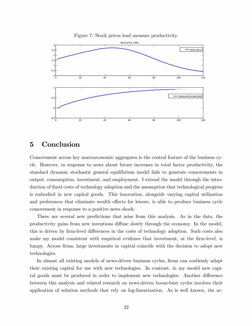
Figure 7: Stock prices lead measure productivity.

0 20 40 60 80 100 1200

0.5

1

1.5

2

2.5

3 stock price index

stock price

0 20 40 60 80 100 120­0.5

0

0.5

1

measured productivity

5 Conclusion

Comovement across key macroeconomic aggregates is the central feature of the business cy-

cle. However, in response to news about future increases in total factor productivity, the

standard dynamic stochastic general equilibrium model fails to generate comovements in

output, consumption, investment, and employment. I extend the model through the intro-

duction of �xed costs of technology adoption and the assumption that technological progress

is embodied in new capital goods. This innovation, alongside varying capital utilization

and preferences that eliminate wealth e¤ects for leisure, is able to produce business cycle

comovement in response to a positive news shock.

There are several new predictions that arise from this analysis. As in the data, the

productivity gains from new inventions di¤use slowly through the economy. In the model,

this is driven by �rm-level di¤erences in the costs of technology adoption. Such costs also

make my model consistent with empirical evidence that investment, at the �rm-level, is

lumpy. Across �rms, large investments in capital coincide with the decision to adopt new

technologies.

In almost all existing models of news-driven business cycles, �rms can costlessly adapt

their existing capital for use with new technologies. In contrast, in my model new capi-

tal goods must be produced in order to implement new technologies. Another di¤erence

between this analysis and related research on news-driven boom-bust cycles involves their

application of solution methods that rely on log-linearization. As is well known, the ac-

22

curacy of such linear methods falls when applied far from the original steady state of a

model. My paper instead relies on nonlinear numerical methods involving value function

approximation; as these are global methods, they do su¤er from accuracy problems when

confronted with large shocks. Finally, while I only study a single discrete jump in the level

of capital-embodied technology, it is straightforward to extend the model to incorporate

ongoing stochastic changes in capital-embodied technology.

While the di¤usion of new technology is fairly rapid here, many microeconomic studies

�nd that actual patterns of technology adoption follow an S-shape. Initially, following a new

invention, a small fraction of �rms adopt the new technology, some time later there is an

episode of rapid adoption and the technology becomes widespread. One possible extension

of the current model involves the introduction of network e¤ects associated with adopting

new technologies. Speci�cally, the bene�t of the new technology for each �rm may rise with

the number of �rms using it. This type of externality may be able to produce the S-shaped

patterns of di¤usion found in empirical micro studies.

References

[1] Atkeson, Andrew, and Kehoe, Patrick J. 2001, "The transition to a new economy after

the Second Industrial Revolution," NBER Working Paper 8676.

[2] Atkeson, Andrew, and Kehoe, Patrick J. 2007, "Modeling the Transition to a New

Economy: Lessons from Two Technological Revolutions," American Economic Review

97(1),64-88.

[3] Bahk, B.-H and M. Gort (1993), "Decomposing learning by doing in plants," Journal

of Political Economy 101, 561-583.

[4] Baxter, M. and D. Farr (2001), �Variable factor utilization and international business

cycles,�NBER Working Paper # 8392.

[5] Beaudry, P. and F. Portier, 2004, �An Exploration into Pigou�s Theory of Cycles?�

Journal of Monetary Economics 51, 1183-1216.

[6] Beaudry, P. and F. Portier, 2006, �News, Stock Prices and Economic Fluctuations,�

American Economic Review 96(4), 1293-1307.

[7] Beaudry, P. and F. Portier, 2007, �When Can Changes in Expectations Cause Business

Cycle Fluctuations in Neo-Classical Settings?�Journal of Economics Theory 135, 458-

477.

23

[8] Barsky, R. and E. Sims (2009) �Information, Animal Spirits, and the Meaning of Inno-

vations in Consumer Con�dence,�NBER Working Paper 15049.

[9] Boddy, Raford and Gort, Michael, 1974, "Obsolescence, Embodiment, and the Expla-

nation of Productivity Change," Southern Economic Journal, 40(4), 553-562.

[10] Campbell, J. R., 1998, "Entry, exit, technology, and business cycles," Review of Eco-

nomic Dynamics, 1, 371-408.

[11] Cooley, Thomas F., Jeremy Greenwood, and Mehmet Yorukoglu, 1997, "The Replace-

ment Problem," Journal of Monetary Economics, 40(3), 457-99.

[12] Cooper, Russell, Haltiwanger, John and Power, Laura, 1999, �Machine Replacement

and the Business Cycle: Lumps and Bumps,�American Economic Review, 89(4), 921-

946.

[13] Christiano, Lawrence J., Eichenbaum Martin, and Evans Charles L., 2005, "Nominal

Rigidities and the Dynamic E¤ects of a Shock to Monetary Policy," Journal of Political

Economy, 113, 1-45.

[14] Christiano, L., C. Ilut, R. Motto, and M. Rostagno, 2007, �Monetary Policy and a Stock

Market Boom-Bust Cycle,�working paper, Northwestern University.

[15] Comin, Diego, Gertler, Mark and Santacreu, Ana Maria, 2008, �News, technology adop-

tion and economic �uctuations�working paper.

[16] Cochrane, John H, 1994, "Shocks," Carnegie�Rochester Conference Series on Public

Policy, 41, pp. 295�364.

[17] Cooley, T. F., Greenwood, J., and Yorukoglu, M., 1997, "The replacement problem,"

Journal of Monetary Economics, 457-499.

[18] David, Paul A., 1990, "The Dynamo and the Computer: An Historical Perspective on

the Modern Productivity Paradox," American Economic Review, 80(2), 355-61.

[19] David, Paul A., 1991, "Computer and Dynamo: The Modern Productivity Paradox in a

Not-Too Distant Mirror," In Technology and Productivity: The Challenge for Economic

Policy, 315-45. Paris: Organisation for Economic Co-operation and Development.

[20] David, Paul A., and Gavin Wright, 1999, "General Purpose Technologies and Surges in

Productivity: Historical Re�ections on the Future of the ICT Revolution," Standford

University Department of Economics Working Paper 99-026.

24

[21] Devine, Warren D., Jr. 1983, "From Shafts to Wires: Historical Perspective on Electri-

�cation," Journal of Economic History, 43(2):347-72.

[22] Doms, M., Dunne, T., 1998, "Capital adjustment patterns in manufacturing plants,"

Review of Economic Dynamics, 1, 409-29.

[23] Eric Sims, 2008, �Expectations Driven Business Cycles: An Empirical Evaluation,�

working paper, University of Michigan.

[24] Erik Brynjolfsson, 1993, "The Productivity Paradox of Information Technology: Review

and Assessment," Communications of the ACM, 36(12), 66-77.

[25] Greenwood, Jeremy, Hercowitz, Zvi and Hu¤man, Gregory W, 1988, "Investment, Ca-

pacity Utilization, and the Real Business Cycle," American Economic Review, 78(3),

402-17.

[26] Greenwood, Jeremy, Hercowitz, Zvi and Krusell, P., 1996, "Long-run implications of

investment-speci�c technological change," American Economic Review, 87, 342-362.

[27] Jaimovich, N. and S. Rebelo, 2008, "Can News about the Future Drive the Business

Cycle?" working paper, Northwestern University.

[28] Jovanovic, Boyan, and Saul Lach, 1989, "Entry, Exit and Di¤usion with Learning by

Doing," American Economic Review, 79(4):690-99.

[29] Jovanovic, Boyan, and Yaw Nyarko, 1995, "A Bayesian Learning Model Fitted to a

Variety of Empirical Learning Curves," Brookings Papers on Economic Activity, Micro-

economics: 247-99.

[30] Jovanovic, Boyan, and Yaw Nyarko, 1996, "Learning by Doing and the choice of tech-

nology," Econometrica, 64, 1299-1310.

[31] Jovanovic, Boyan, and Peter L. Rousseau, 2005, "General Purpose Technologies," Na-

tional Bureau of Economic Research Working Paper 11093.

[32] Khan, Aubhik and Ravikumar, B., 2002, "Costly Technology Adoption and Capital

Accumulation," Review of Economic Dynamics, 5(2), 489-502.

[33] Khan, Aubhik and Thomas, Julia K., 2003, "Nonconvex factor adjustments in equilib-

rium business cycle models: do nonlinearities matter?," Journal of Monetary Economics,

50(2), pages 331-360.

25

[34] Rotemberg, Julio, and Michael Woodford, 1997, "An Optimization-Based Econometric

Framework for the Evaluation of Monetary Policy," NBER Macroeconomics Annual,

297-346.

[35] Schmitt-Grohe, Stephanie and Uribe, Martin, 2008, "What�s News In Business Cycles,"

NBER Working Papers 14215.

[36] Schurr, Sam H., Calvin C. Burwell, Warren D. Devine, Jr., and Sidney Sonenblum.

1990. Electricity in the American Economy: Agent of Technological Progress. Westport:

Greenwood Press.

[37] Schurr, Sam H., Bruce C. Netschert, Vera Eliasberg, Joseph Lerner, and Hans H. Lands-

berg. 1960. Energy in the American Economy, 1850-1975: An Economy Study of Its

History and Prospects. Baltimore: John Hopkins University Press.

26