Embed Size (px)
Citation preview

Newtonian Dynamics
Richard Fitzpatrick
Professor of Physics
The University of Texas at Austin

For Faith
CONTENTS 3
Contents
1 Introduction 9
1.1 Prerequisites . . . . . . . . . . . . . . . . . . . . . . . . . . . 9
1.2 Scope of Book . . . . . . . . . . . . . . . . . . . . . . . . . . 9
1.3 Major Sources . . . . . . . . . . . . . . . . . . . . . . . . . . 11
2 Vector Algebra and Vector Calculus 13
2.1 Introduction . . . . . . . . . . . . . . . . . . . . . . . . . . . 13
2.2 Vector Algebra . . . . . . . . . . . . . . . . . . . . . . . . . . 13
2.3 Scalar Product . . . . . . . . . . . . . . . . . . . . . . . . . . 16
2.4 Vector Product . . . . . . . . . . . . . . . . . . . . . . . . . . 19
2.5 Rotation . . . . . . . . . . . . . . . . . . . . . . . . . . . . . 22
2.6 Scalar Triple Product . . . . . . . . . . . . . . . . . . . . . . 24
2.7 Vector Triple Product . . . . . . . . . . . . . . . . . . . . . . 25
2.8 Vector Calculus . . . . . . . . . . . . . . . . . . . . . . . . . 26
2.9 Line Integrals . . . . . . . . . . . . . . . . . . . . . . . . . . 26
2.10 Vector Line Integrals . . . . . . . . . . . . . . . . . . . . . . 29
2.11 Volume Integrals . . . . . . . . . . . . . . . . . . . . . . . . 30
2.12 Gradient . . . . . . . . . . . . . . . . . . . . . . . . . . . . . 31
2.13 Exercises . . . . . . . . . . . . . . . . . . . . . . . . . . . . . 36
3 Fundamental Concepts 39
3.1 Introduction . . . . . . . . . . . . . . . . . . . . . . . . . . . 39
3.2 Fundamental Assumptions . . . . . . . . . . . . . . . . . . . 39
3.3 Newton’s Laws of Motion . . . . . . . . . . . . . . . . . . . . 41
3.4 Newton’s First Law of Motion . . . . . . . . . . . . . . . . . 41
3.5 Newton’s Second Law of Motion . . . . . . . . . . . . . . . . 44
3.6 Newton’s Third Law of Motion . . . . . . . . . . . . . . . . . 46
3.7 Exercises . . . . . . . . . . . . . . . . . . . . . . . . . . . . . 49
4 One-Dimensional Motion 51
4.1 Introduction . . . . . . . . . . . . . . . . . . . . . . . . . . . 51
4.2 Motion in a General One-Dimensional Potential . . . . . . . 51
4.3 Velocity Dependent Forces . . . . . . . . . . . . . . . . . . . 54
4.4 Simple Harmonic Motion . . . . . . . . . . . . . . . . . . . . 57
4.5 Damped Oscillatory Motion . . . . . . . . . . . . . . . . . . 59
4.6 Quality Factor . . . . . . . . . . . . . . . . . . . . . . . . . . 62
4.7 Resonance . . . . . . . . . . . . . . . . . . . . . . . . . . . . 64
4.8 Periodic Driving Forces . . . . . . . . . . . . . . . . . . . . . 66

4 NEWTONIAN DYNAMICS
4.9 Transients . . . . . . . . . . . . . . . . . . . . . . . . . . . . 70
4.10 Simple Pendulum . . . . . . . . . . . . . . . . . . . . . . . . 71
4.11 Exercises . . . . . . . . . . . . . . . . . . . . . . . . . . . . . 74
5 Multi-Dimensional Motion 77
5.1 Introduction . . . . . . . . . . . . . . . . . . . . . . . . . . . 77
5.2 Motion in a Two-Dimensional Harmonic Potential . . . . . . 77
5.3 Projectile Motion with Air Resistance . . . . . . . . . . . . . 80
5.4 Charged Particle Motion in Electric and Magnetic Fields . . . 84
5.5 Exercises . . . . . . . . . . . . . . . . . . . . . . . . . . . . . 86
6 Planetary Motion 89
6.1 Introduction . . . . . . . . . . . . . . . . . . . . . . . . . . . 89
6.2 Kepler’s Laws . . . . . . . . . . . . . . . . . . . . . . . . . . 89
6.3 Newtonian Gravity . . . . . . . . . . . . . . . . . . . . . . . 89
6.4 Conservation Laws . . . . . . . . . . . . . . . . . . . . . . . 90
6.5 Plane Polar Coordinates . . . . . . . . . . . . . . . . . . . . 91
6.6 Conic Sections . . . . . . . . . . . . . . . . . . . . . . . . . . 94
6.7 Kepler’s Second Law . . . . . . . . . . . . . . . . . . . . . . 97
6.8 Kepler’s First Law . . . . . . . . . . . . . . . . . . . . . . . . 98
6.9 Kepler’s Third Law . . . . . . . . . . . . . . . . . . . . . . . 99
6.10 Orbital Energies . . . . . . . . . . . . . . . . . . . . . . . . . 100
6.11 Kepler Problem . . . . . . . . . . . . . . . . . . . . . . . . . 102
6.12 Motion in a General Central Force-Field . . . . . . . . . . . . 105
6.13 Motion in a Nearly Circular Orbit . . . . . . . . . . . . . . . 106
6.14 Exercises . . . . . . . . . . . . . . . . . . . . . . . . . . . . . 109
7 Two-Body Dynamics 111
7.1 Introduction . . . . . . . . . . . . . . . . . . . . . . . . . . . 111
7.2 Reduced Mass . . . . . . . . . . . . . . . . . . . . . . . . . . 111
7.3 Binary Star Systems . . . . . . . . . . . . . . . . . . . . . . . 112
7.4 Scattering in the Center of Mass Frame . . . . . . . . . . . . 114
7.5 Scattering in the Laboratory Frame . . . . . . . . . . . . . . 120
7.6 Exercises . . . . . . . . . . . . . . . . . . . . . . . . . . . . . 126
8 Non-Inertial Reference Frames 129
8.1 Introduction . . . . . . . . . . . . . . . . . . . . . . . . . . . 129
8.2 Rotating Reference Frames . . . . . . . . . . . . . . . . . . . 129
8.3 Centrifugal Acceleration . . . . . . . . . . . . . . . . . . . . 131
8.4 Coriolis Force . . . . . . . . . . . . . . . . . . . . . . . . . . 134

CONTENTS 5
8.5 Foucault Pendulum . . . . . . . . . . . . . . . . . . . . . . . 137
8.6 Exercises . . . . . . . . . . . . . . . . . . . . . . . . . . . . . 139
9 Rigid Body Rotation 141
9.1 Introduction . . . . . . . . . . . . . . . . . . . . . . . . . . . 141
9.2 Fundamental Equations . . . . . . . . . . . . . . . . . . . . . 141
9.3 Moment of Inertia Tensor . . . . . . . . . . . . . . . . . . . . 142
9.4 Rotational Kinetic Energy . . . . . . . . . . . . . . . . . . . . 144
9.5 Matrix Eigenvalue Theory . . . . . . . . . . . . . . . . . . . 145
9.6 Principal Axes of Rotation . . . . . . . . . . . . . . . . . . . 147
9.7 Euler’s Equations . . . . . . . . . . . . . . . . . . . . . . . . 150
9.8 Eulerian Angles . . . . . . . . . . . . . . . . . . . . . . . . . 153
9.9 Gyroscopic Precession . . . . . . . . . . . . . . . . . . . . . 159
9.10 Rotational Stability . . . . . . . . . . . . . . . . . . . . . . . 162
9.11 Exercises . . . . . . . . . . . . . . . . . . . . . . . . . . . . . 165
10 Lagrangian Dynamics 167
10.1 Introduction . . . . . . . . . . . . . . . . . . . . . . . . . . . 167
10.2 Generalized Coordinates . . . . . . . . . . . . . . . . . . . . 167
10.3 Generalized Forces . . . . . . . . . . . . . . . . . . . . . . . 168
10.4 Lagrange’s Equation . . . . . . . . . . . . . . . . . . . . . . . 169
10.5 Motion in a Central Potential . . . . . . . . . . . . . . . . . . 171
10.6 Atwood Machines . . . . . . . . . . . . . . . . . . . . . . . . 172
10.7 Sliding down a Sliding Plane . . . . . . . . . . . . . . . . . . 175
10.8 Generalized Momenta . . . . . . . . . . . . . . . . . . . . . 176
10.9 Spherical Pendulum . . . . . . . . . . . . . . . . . . . . . . . 178
10.10 Exercises . . . . . . . . . . . . . . . . . . . . . . . . . . . . . 180
11 Hamiltonian Dynamics 183
11.1 Introduction . . . . . . . . . . . . . . . . . . . . . . . . . . . 183
11.2 Calculus of Variations . . . . . . . . . . . . . . . . . . . . . . 183
11.3 Conditional Variation . . . . . . . . . . . . . . . . . . . . . . 186
11.4 Multi-Function Variation . . . . . . . . . . . . . . . . . . . . 188
11.5 Hamilton’s Principle . . . . . . . . . . . . . . . . . . . . . . . 189
11.6 Constrained Lagrangian Dynamics . . . . . . . . . . . . . . . 189
11.7 Hamilton’s Equations . . . . . . . . . . . . . . . . . . . . . . 194
11.8 Exercises . . . . . . . . . . . . . . . . . . . . . . . . . . . . . 197
12 Coupled Oscillations 199
12.1 Introduction . . . . . . . . . . . . . . . . . . . . . . . . . . . 199

6 NEWTONIAN DYNAMICS
12.2 Equilibrium State . . . . . . . . . . . . . . . . . . . . . . . . 199
12.3 Stability Equations . . . . . . . . . . . . . . . . . . . . . . . 200
12.4 More Matrix Eigenvalue Theory . . . . . . . . . . . . . . . . 202
12.5 Normal Modes . . . . . . . . . . . . . . . . . . . . . . . . . . 203
12.6 Normal Coordinates . . . . . . . . . . . . . . . . . . . . . . . 205
12.7 Spring-Coupled Masses . . . . . . . . . . . . . . . . . . . . . 207
12.8 Triatomic Molecule . . . . . . . . . . . . . . . . . . . . . . . 209
12.9 Exercises . . . . . . . . . . . . . . . . . . . . . . . . . . . . . 212
13 Gravitational Potential Theory 215
13.1 Introduction . . . . . . . . . . . . . . . . . . . . . . . . . . . 215
13.2 Gravitational Potential . . . . . . . . . . . . . . . . . . . . . 215
13.3 Axially Symmetric Mass Distributions . . . . . . . . . . . . . 216
13.4 Potential Due to a Uniform Sphere . . . . . . . . . . . . . . . 219
13.5 Potential Outside a Uniform Spheroid . . . . . . . . . . . . . 220
13.6 Rotational Flattening . . . . . . . . . . . . . . . . . . . . . . 223
13.7 McCullough’s Formula . . . . . . . . . . . . . . . . . . . . . 225
13.8 Tidal Elongation . . . . . . . . . . . . . . . . . . . . . . . . . 226
13.9 Roche Radius . . . . . . . . . . . . . . . . . . . . . . . . . . 232
13.10 Precession of the Equinoxes . . . . . . . . . . . . . . . . . . 234
13.11 Potential Due to a Uniform Ring . . . . . . . . . . . . . . . . 240
13.12 Perihelion Precession of the Planets . . . . . . . . . . . . . . 241
13.13 Perihelion Precession of Mercury . . . . . . . . . . . . . . . . 243
13.14 Exercises . . . . . . . . . . . . . . . . . . . . . . . . . . . . . 246
14 The Three-Body Problem 247
14.1 Introduction . . . . . . . . . . . . . . . . . . . . . . . . . . . 247
14.2 Circular Restricted Three-Body Problem . . . . . . . . . . . . 247
14.3 Jacobi Integral . . . . . . . . . . . . . . . . . . . . . . . . . . 249
14.4 Tisserand Criterion . . . . . . . . . . . . . . . . . . . . . . . 249
14.5 Co-Rotating Frame . . . . . . . . . . . . . . . . . . . . . . . 251
14.6 Lagrange Points . . . . . . . . . . . . . . . . . . . . . . . . . 253
14.7 Zero-Velocity Surfaces . . . . . . . . . . . . . . . . . . . . . 256
14.8 Stability of Lagrange Points . . . . . . . . . . . . . . . . . . 259
15 The Chaotic Pendulum 267
15.1 Introduction . . . . . . . . . . . . . . . . . . . . . . . . . . . 267
15.2 Basic Problem . . . . . . . . . . . . . . . . . . . . . . . . . . 267
15.3 Analytic Solution . . . . . . . . . . . . . . . . . . . . . . . . 269
15.4 Numerical Solution . . . . . . . . . . . . . . . . . . . . . . . 274

CONTENTS 7
15.5 Poincare Section . . . . . . . . . . . . . . . . . . . . . . . . . 274
15.6 Spatial Symmetry Breaking . . . . . . . . . . . . . . . . . . . 277
15.7 Basins of Attraction . . . . . . . . . . . . . . . . . . . . . . . 281
15.8 Period-Doubling Bifurcations . . . . . . . . . . . . . . . . . . 286
15.9 Route to Chaos . . . . . . . . . . . . . . . . . . . . . . . . . 290
15.10 Sensitivity to Initial Conditions . . . . . . . . . . . . . . . . 296
15.11 Definition of Chaos . . . . . . . . . . . . . . . . . . . . . . . 302
15.12 Periodic Windows . . . . . . . . . . . . . . . . . . . . . . . . 302
15.13 Further Investigation . . . . . . . . . . . . . . . . . . . . . . 307

8 NEWTONIAN DYNAMICS

Introduction 9
1 Introduction
1.1 Prerequisites
This book presents a single semester course on Newtonian Dynamics which
is primarily intended for upper-division undergraduate students majoring in
Physics. An understanding of the latter discipline at the lower-division level,
including a basic working knowledge of the laws of mechanics, is assumed.
It is also taken for granted that the student is familiar with the fundamentals
of calculus, linear ordinary differential equation theory, and linear algebra.
On the other hand, vector analysis plays such a central role in the study
of Newtonian Dynamics that a brief, but fairly comprehensive, review of
this subject area is provided in Chapter 2. Likewise, those results in matrix
eigenvalue theory which are helpful in the analysis of rigid body motion
and coupled oscillations are derived in Sections 9.5 and 12.4, respectively.
Finally, the calculus of variations, an area of Mathematics which is central
to Hamiltonian dynamics, is outlined in Section 11.2.
1.2 Scope of Book
The scope of this book is indicated by its title, “Newtonian Dynamics”. Tak-
ing the elements of this title in reverse order: “Dynamics” is the study of the
motions of the various objects in the world around us; and by “Newtonian”,
we understand that the theory which we are actually going to employ in
our investigation of Dynamics is that which was first formulated by Sir Isaac
Newton in 1687. We now know that this theory is only approximately true.
The theory breaks down, due to relativistic effects, when the velocities of
the objects under investigation approach the speed of light in vacuum, and
in regions of space in which the underlying geometry is not approximately
Euclidean. The theory also breaks down on atomic and subatomic length-
scales, and must be replaced by Quantum Mechanics. In this book, we shall
entirely neglect relativistic and quantum mechanical effects. It follows that
we must restrict our investigations to the dynamics of large (compared to an
atom), slowly moving (compared to the velocity of light), objects in Euclidean
space. Fortunately, the vast majority of the motions which we commonly ob-
serve in the world around us fall into this category.
For the sake of simplicity, and brevity, we shall restrict our investigations

10 NEWTONIAN DYNAMICS
to the motions of idealized point particles and idealized rigid bodies. To be
more exact, we shall exclude from consideration any discussion of statics,
the strength of materials, and the non-rigid motions of continuous media.
We shall also concentrate, for the most part, on motions which take place
under the influence of conservative forces, such as gravity, which can be accu-
rately represented in terms of simple mathematical formulae. Finally, with
one exception, we shall only consider that subset of dynamical problems
that can be solved by means of conventional mathematical analysis.
Newtonian Dynamics was originally developed in order to predict the
motions of the objects which make up the Solar System. It turns out that
this is an ideal application of the theory, since quantum mechanical and rel-
ativistic effects are (mostly) irrelevant, the objects in question can be mod-
eled as being rigid to a fair degree of accuracy, and the motions take place
under the action of a single conservative force—namely, gravity—which has
a simple mathematical form. In particular, the frictional forces which greatly
complicate the application of Newtonian Dynamics to the motions of every-
day objects close to the Earth’s surface are completely absent. In this book,
we shall make a particular effort to describe how Newtonian Dynamics can
successfully account for a wide variety of different Solar System phenom-
ena. For example, we shall explain the origins of Kepler’s laws of planetary
motion (see Chapter 6), the rotational flattening of the Earth, the tides, the
Roche radius (i.e., the minimum radius at which a moon can orbit a planet
without being destroyed by tidal forces), the precession of the equinoxes,
and the perihelion precession of the planets (see Chapter 13). We shall also
derive the Tisserand criterion used to re-identify comets whose orbits have
been modified by close encounters with massive planets, and account for the
existence of the so-called Trojan asteroids which share the orbit of Jupiter
(see Chapter 14).
Virtually all of the results described in this book were first obtained ei-
ther by Newton himself, or by scientists living in the 150, or so, years im-
mediately following the initial publication of his theory, using conventional
mathematical analysis. Indeed, scientists at the beginning of the 20th cen-
tury generally assumed that they knew everything that there was to known
about Newtonian Dynamics. However, they were wrong. The advent of fast
electronic computers, in the latter half of the 20th century, allowed scien-
tists to solve nonlinear equations of motion, for the first time, via numerical
techniques. In general, such equations are insoluble using standard analytic
methods. The numerical investigation of dynamical systems with nonlinear
equations of motion revealed the existence of a previously unknown type
of motion known as deterministic chaos. Such motion is quasi-random (de-

Introduction 11
spite being derived from deterministic equations of motion), aperiodic, and
exhibits extreme sensitivity to initial conditions. The discovery of chaotic
motion lead to a renaissance in the study of Newtonian Dynamics which
started in the late 20th century and is still ongoing. It is therefore appro-
priate that the last chapter in this book is devoted to an in-depth numerical
investigation of a particular dynamical system which exhibits chaotic motion
(see Chapter 15).
1.3 Major Sources
The material appearing in Chapter 2 is largely based on the author’s recollec-
tions of a vector analysis course given by Dr. Stephen Gull at the University
of Cambridge. Major sources for the material appearing in Chapters 3–
14 include Analytical Mechanics, G.R. Fowles (Holt, Rinehart, and Winston,
New York NY, 1977); Solar System Dynamics, C.D. Murray, and S.F. Der-
mott (Cambridge University Press, Cambridge UK, 1999); Classical Mechan-
ics, 3rd Edition, H. Goldstein, C. Poole, and J. Safko (Addison-Wesley, San
Fransico CA, 2002); Classical Dynamics of Particles and Systems, 5th Edition,
S.T. Thornton, and J.B. Marion (Brooks/Cole—Thomson Learning, Belmont
CA, 2004); and Analytical Mechanics, 7th Edition, G.R. Fowles, and G.L. Cas-
siday (Brooks/Cole—Thomson Learning, Belmont CA, 2005). The various
sources for the material appearing in Chapter 15 are identified in footnotes.

12 NEWTONIAN DYNAMICS

Vector Algebra and Vector Calculus 13
2 Vector Algebra and Vector Calculus
2.1 Introduction
This chapter briefly outlines those aspects of Vector Algebra and Vector Cal-
culus which are helpful in the study of Newtonian Dynamics. The essential
purpose of Vector Algebra is to convert the propositions of Euclidean Ge-
ometry in three-dimensional space into a convenient algebraic form. Vector
Calculus allows us to define the instantaneous velocity and acceleration of a
moving point in three-dimensional space, as well as the distance moved by
such a point, in a given time interval, along a general curved trajectory. Vec-
tor Calculus also introduces the concept of a scalar field: e.g., the potential
energy associated with a conservative force.
2.2 Vector Algebra
In Newtonian Dynamics, physical quantities are (predominately) represented
by two distinct classes of objects. Some quantities, denoted scalars, are
represented by real numbers. Others, denoted vectors, are represented by
directed line elements in space: e.g.,→PQ—see Figure 2.1. Note that line
elements (and, therefore, vectors) are movable, and do not carry intrin-
sic position information: i.e., in Figure 2.2,→PS and
→QR are considered to
be the same vector. In fact, vectors just possess a magnitude and a direc-
tion, whereas scalars possess a magnitude but no direction. By convention,
vector quantities are denoted by bold-faced characters (e.g., a) in typeset
documents. Vector addition can be represented using a parallelogram: e.g.,
P
Q
Figure 2.1: A directed line element.

14 NEWTONIAN DYNAMICS
c
P
S
R
Q
b
a
a
b
Figure 2.2: Vector addition.
→PR=
→PQ +
→QR—see Figure 2.2. Suppose that a ≡
→PQ≡
→SR, b ≡
→QR≡
→PS,
and c ≡→PR. It is clear, from Figure 2.2, that vector addition is commutative:
i.e., c = a + b = b + a. It can also be shown that the associative law holds:
i.e., a + (b + c) = (a + b) + c.
There are two main approaches to vector algebra. The geometric ap-
proach is based on line elements in space. The coordinate approach assumes
that space is defined in terms of Cartesian coordinates, and uses these to
characterize vectors. In Newtonian Dynamics, we generally adopt the sec-
ond approach, because it is far more convenient than the first.
In the coordinate approach, a vector is denoted as the row matrix of its
components (i.e., perpendicular projections) along each of three mutually
perpendicular Cartesian axes (the x-, y-, and z-axes, say): e.g.,
a ≡ (ax, ay, az). (2.1)
If a ≡ (ax, ay, az) and b ≡ (bx, by, bz) then vector addition is defined
a + b ≡ (ax+ bx, ay+ by, az+ bz). (2.2)
If a is a vector and n is a scalar then the product of a scalar and a vector is
defined
n a ≡ (nax, n ay, n az). (2.3)
Note that n a is interpreted as a vector which is parallel (or anti-parallel if
n < 0) to a, and of length |n| times that of a. It is clear that vector algebra is
distributive with respect to scalar multiplication: i.e., n (a + b) = n a + nb.

Vector Algebra and Vector Calculus 15
It is also easily demonstrated that (n + m) a = n a + m a, and n (m a) =
(nm) a, where m is a second scalar.
Unit vectors can be defined in the x-, y-, and z-directions as ex ≡ (1, 0, 0),
ey ≡ (0, 1, 0), and ez ≡ (0, 0, 1). Any vector can be written in terms of these
unit vectors: e.g.,
a = axex+ ayey+ azez. (2.4)
In mathematical terminology, three vectors used in this manner form a basis
of the vector space. If the three vectors are mutually perpendicular then they
are termed orthogonal basis vectors. However, any set of three non-coplanar
vectors can be used as basis vectors.
Common examples of vectors in Newtonian Dynamics are displacements
from an origin,
r = (x, y, z), (2.5)
velocities (see Section 2.8),
v =dr
dt= limδt→0
r(t+ δt) − r(t)
δt, (2.6)
and accelerations
a =dv
dt= limδt→0
v(t+ δt) − v(t)
δt. (2.7)
Suppose that we transform to a new orthogonal basis, the x ′-, y ′-, and
z ′-axes, which are related to the x-, y-, and z-axes via a rotation through an
angle θ around the z-axis—see Figure 2.3. In the new basis, the coordinates
of the general displacement r from the origin are (x ′, y ′, z ′). According to
simple trigonometry, these coordinates are related to the previous coordi-
nates via the transformation:
x ′ = x cosθ+ y sin θ, (2.8)
y ′ = −x sin θ+ y cos θ, (2.9)
z ′ = z. (2.10)
We do not need to change our notation for the displacement in the new
basis. It is still denoted r. The reason for this is that the magnitude and
direction of r are independent of the choice of basis vectors. The coordinates
of r do depend on the choice of basis vectors. However, they must depend
in a very specific manner [i.e., Equations (2.8)–(2.10)] which preserves the
magnitude and direction of r.

16 NEWTONIAN DYNAMICS
⊙ zy′y
x′
xθ
Figure 2.3: Rotation of the basis about the z-axis.
Since any vector can be represented as a displacement from an origin
(because this is just a special case of a directed line element), it follows
that the components of a general vector a must transform in an analogous
manner to Equations (2.8)–(2.10). Thus,
ax′ = ax cos θ+ ay sin θ, (2.11)
ay′ = −ax sin θ+ ay cosθ, (2.12)
az′ = az, (2.13)
with analogous transformation rules for rotation about the y- and z-axes. In
the coordinate approach, Equations (2.11)–(2.13) constitute the definition
of a vector. The three quantities (ax, ay, az) are the components of a vector
provided that they transform under rotation like Equations (2.11)–(2.13).
Conversely, (ax, ay, az) cannot be the components of a vector if they do not
transform like Equations (2.11)–(2.13). Scalar quantities are invariant un-
der transformation. Thus, the individual components of a vector (ax, say)
are real numbers, but they are not scalars. Displacement vectors, and all
vectors derived from displacements, automatically satisfy Equations (2.11)–
(2.13). There are, however, other physical quantities which have both mag-
nitude and direction, but which are not obviously related to displacements.
We need to check carefully to see whether these quantities are vectors (see
Section 2.5).
2.3 Scalar Product
A scalar quantity is invariant under all possible rotational transformations.
The individual components of a vector are not scalars because they change
under transformation. Can we form a scalar out of some combination of the

Vector Algebra and Vector Calculus 17
components of one, or more, vectors? Suppose that we were to define the
“percent” product,
a % b = axbz+ aybx+ azby = scalar number, (2.14)
for general vectors a and b. Is a % b invariant under transformation, as
must be the case if it is a scalar number? Let us consider an example. Sup-
pose that a = (0, 1, 0) and b = (1, 0, 0). It is easily seen that a % b = 1.
Let us now rotate the basis through 45 about the z-axis. In the new ba-
sis, a = (1/√2, 1/
√2, 0) and b = (1/
√2, −1/
√2, 0), giving a % b = 1/2.
Clearly, a % b is not invariant under rotational transformation, so the above
definition is a bad one.
Consider, now, the dot product or scalar product:
a · b = axbx+ ayby+ azbz = scalar number. (2.15)
Let us rotate the basis though θ degrees about the z-axis. According to
Equations (2.11)–(2.13), in the new basis a · b takes the form
a · b = (ax cos θ+ ay sin θ) (bx cos θ+ by sin θ)
+(−ax sin θ+ ay cos θ) (−bx sin θ+ by cosθ) + azbz
= axbx+ ayby+ azbz. (2.16)
Thus, a·b is invariant under rotation about the z-axis. It can easily be shown
that it is also invariant under rotation about the x- and y-axes. Clearly, a · b
is a true scalar, so the above definition is a good one. Incidentally, a ·b is the
only simple combination of the components of two vectors which transforms
like a scalar. It is easily shown that the dot product is commutative and
distributive: i.e.,
a · b = b · a,
a · (b + c) = a · b + a · c. (2.17)
The associative property is meaningless for the dot product, because we
cannot have (a · b) · c, since a · b is scalar.
We have shown that the dot product a ·b is coordinate independent. But
what is the geometric significance of this? Consider the special case where
a = b. Clearly,
a · b = a 2x + a 2y + a 2z = Length (OP)2, (2.18)

18 NEWTONIAN DYNAMICS
b − a
Oθ
A
B
.
b
a
Figure 2.4: A vector triangle.
if a is the position vector of P relative to the origin O. So, the invariance of
a · a is equivalent to the invariance of the length, or magnitude, of vector
a under transformation. The length of vector a is usually denoted |a| (“the
modulus of a”) or sometimes just a, so
a · a = |a|2 = a2. (2.19)
Let us now investigate the general case. The length squared of AB in the
vector triangle shown in Figure 2.4 is
(b − a) · (b − a) = |a|2+ |b|2− 2 a · b. (2.20)
However, according to the “cosine rule” of trigonometry,
(AB)2 = (OA)2+ (OB)2− 2 (OA) (OB) cos θ, (2.21)
where (AB) denotes the length of side AB. It follows that
a · b = |a| |b| cos θ. (2.22)
Clearly, the invariance of a · b under transformation is equivalent to the
invariance of the angle subtended between the two vectors. Note that if
a ·b = 0 then either |a| = 0, |b| = 0, or the vectors a and b are perpendicular.
The angle subtended between two vectors can easily be obtained from the
dot product:
cos θ =a · b
|a| |b|. (2.23)
The workW performed by a constant force F moving an object through a
displacement r is the product of the magnitude of F times the displacement
in the direction of F. If the angle subtended between F and r is θ then
W = |F| (|r| cos θ) = F · r. (2.24)

Vector Algebra and Vector Calculus 19
The work dW performed by a non-constant force f which moves an
object through an infinitesimal displacement dr in a time interval dt is
dW = f · dr. Thus, the rate at which the force does work on the object,
which is usually referred to as the power, is P = dW/dt = f · dr/dt, or
P = f · v, where v = dr/dt is the object’s instantaneous velocity.
2.4 Vector Product
We have discovered how to construct a scalar from the components of two
general vectors a and b. Can we also construct a vector which is not just a
linear combination of a and b? Consider the following definition:
a ∗ b = (axbx, ayby, azbz). (2.25)
Is a ∗ b a proper vector? Suppose that a = (0, 1, 0), b = (1, 0, 0). Clearly,
a ∗ b = 0. However, if we rotate the basis through 45 about the z-axis then
a = (1/√2, 1/
√2, 0), b = (1/
√2, −1/
√2, 0), and a ∗ b = (1/2, −1/2, 0).
Thus, a ∗ b does not transform like a vector, because its magnitude depends
on the choice of axes. So, above definition is a bad one.
Consider, now, the cross product or vector product:
a × b = (aybz− azby, azbx− axbz, axby− aybx) = c. (2.26)
Does this rather unlikely combination transform like a vector? Let us try ro-
tating the basis through θ degrees about the z-axis using Equations (2.11)–
(2.13). In the new basis,
cx′ = (−ax sin θ+ ay cosθ)bz− az (−bx sin θ+ by cos θ)
= (aybz− azby) cosθ+ (azbx− axbz) sin θ
= cx cos θ+ cy sin θ. (2.27)
Thus, the x-component of a × b transforms correctly. It can easily be shown
that the other components transform correctly as well, and that all compo-
nents also transform correctly under rotation about the y- and z-axes. Thus,
a × b is a proper vector. Incidentally, a × b is the only simple combination
of the components of two vectors that transforms like a vector (which is
non-coplanar with a and b). The cross product is anticommutative,
a × b = −b × a, (2.28)
distributive,
a × (b + c) = a × b + a × c, (2.29)

20 NEWTONIAN DYNAMICS
b
middle finger
index finger
thumb
θ
a × b
a
Figure 2.5: The right-hand rule for cross products. Here, θ is less that 180.
but is not associative,
a × (b × c) 6= (a × b) × c. (2.30)
Note that a × b can be written in the convenient, and easy to remember,
determinant form
a × b =
∣
∣
∣
∣
∣
∣
∣
ex ey ez
ax ay az
bx by bz
∣
∣
∣
∣
∣
∣
∣
. (2.31)
The cross product transforms like a vector, which means that it must
have a well-defined direction and magnitude. We can show that a × b is
perpendicular to both a and b. Consider a · a × b. If this is zero then the
cross product must be perpendicular to a. Now,
a · a × b = ax (aybz− azby) + ay (azbx− axbz) + az (axby− aybx)
= 0. (2.32)
Therefore, a×b is perpendicular to a. Likewise, it can be demonstrated that
a × b is perpendicular to b. The vectors a, b, and a × b form a right-handed
set, like the unit vectors ex, ey, and ez. In fact, ex× ey = ez. This defines a
unique direction for a × b, which is obtained from the right-hand rule—see
Figure 2.5.
Let us now evaluate the magnitude of a × b. We have
(a × b)2 = (aybz− azby)2+ (azbx− axbz)
2+ (axby− aybx)2
= (a 2x + a 2y + a 2z ) (b 2x + b 2y + b 2z ) − (axbx+ ayby+ azbz)2
= |a|2 |b|2− (a · b)2
= |a|2 |b|2− |a|2 |b|2 cos2θ = |a|2 |b|2 sin2θ. (2.33)

Vector Algebra and Vector Calculus 21
Thus,
|a × b| = |a| |b| sin θ, (2.34)
where θ is the angle subtended between a and b. Clearly, a × a = 0 for
any vector, since θ is always zero in this case. Also, if a × b = 0 then either
|a| = 0, |b| = 0, or b is parallel (or antiparallel) to a.
Consider the parallelogram defined by vectors a and b—see Figure 2.6.
The scalar area is ab sin θ. By definition, the vector area has the magnitude
of the scalar area, and is normal to the plane of the parallelogram, which
means that it is perpendicular to both a and b. Clearly, the vector area is
given by
S = a × b, (2.35)
with the sense obtained from the right-hand grip rule by rotating a on to b.
Suppose that a force F is applied at position r—see Figure 2.7. The
torque about the origin O is the product of the magnitude of the force
and the length of the lever arm OQ. Thus, the magnitude of the torque
is |F| |r| sin θ. The direction of the torque is conventionally the direction of
the axis through O about which the force tries to rotate objects, in the sense
determined by the right-hand grip rule. It follows that the vector torque is
given by
τ = r × F. (2.36)
The angular momentum, l, of a particle of linear momentum p and po-
sition vector r is simply defined as the moment of its momentum about the
origin. Hence,
l = r × p. (2.37)
b
a
b
θa
Figure 2.6: A vector parallelogram.

22 NEWTONIAN DYNAMICS
r
O
θ
P
Q
F
r sin θ
Figure 2.7: A torque.
2.5 Rotation
Let us try to define a rotation vector θ whose magnitude is the angle of
the rotation, θ, and whose direction is the axis of the rotation, in the sense
determined by the right-hand grip rule. Unfortunately, this is not a good
vector. The problem is that the addition of rotations is not commutative,
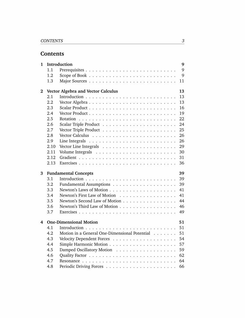
whereas vector addition is commuative. Figure 2.8 shows the effect of ap-
plying two successive 90 rotations, one about x-axis, and the other about
the z-axis, to a standard six-sided die. In the left-hand case, the z-rotation
is applied before the x-rotation, and vice versa in the right-hand case. It
can be seen that the die ends up in two completely different states. Clearly,
the z-rotation plus the x-rotation does not equal the x-rotation plus the z-
rotation. This non-commuting algebra cannot be represented by vectors.
So, although rotations have a well-defined magnitude and direction, they
are not vector quantities.
But, this is not quite the end of the story. Suppose that we take a general
vector a and rotate it about the z-axis by a small angle δθz. This is equiv-
alent to rotating the basis about the z-axis by −δθz. According to Equa-
tions (2.11)–(2.13), we have
a ′ ≃ a + δθzez× a, (2.38)
where use has been made of the small angle approximations sinθ ≃ θ and
cosθ ≃ 1. The above equation can easily be generalized to allow small
rotations about the x- and y-axes by δθx and δθy, respectively. We find that
a ′ ≃ a + δθ × a, (2.39)
Vector Algebra and Vector Calculus 23
x
x-axisz-axis
x-axis z-axis
z
y
Figure 2.8: Effect of successive rotations about perpendicular axes on a six-
sided die.
where
δθ = δθxex+ δθyey+ δθzez. (2.40)
Clearly, we can define a rotation vector δθ, but it only works for small angle
rotations (i.e., sufficiently small that the small angle approximations of sine
and cosine are good). According to the above equation, a small z-rotation
plus a small x-rotation is (approximately) equal to the two rotations applied
in the opposite order. The fact that infinitesimal rotation is a vector implies
that angular velocity,
ω = limδt→0
δθ
δt, (2.41)
must be a vector as well. Also, if a ′ is interpreted as a(t + δt) in Equa-
tion (2.39) then it is clear that the equation of motion of a vector precessing
about the origin with angular velocity ω is
da
dt= ω × a. (2.42)

24 NEWTONIAN DYNAMICS
c
b
a
Figure 2.9: A vector parallelepiped.
2.6 Scalar Triple Product
Consider three vectors a, b, and c. The scalar triple product is defined
a ·b× c. Now, b× c is the vector area of the parallelogram defined by b and
c. So, a · b × c is the scalar area of this parallelogram times the component
of a in the direction of its normal. It follows that a ·b×c is the volume of the
parallelepiped defined by vectors a, b, and c—see Figure 2.9. This volume
is independent of how the triple product is formed from a, b, and c, except
that
a · b × c = −a · c × b. (2.43)
So, the “volume” is positive if a, b, and c form a right-handed set (i.e., if a
lies above the plane of b and c, in the sense determined from the right-hand
grip rule by rotating b onto c) and negative if they form a left-handed set.
The triple product is unchanged if the dot and cross product operators are
interchanged,
a · b × c = a × b · c. (2.44)
The triple product is also invariant under any cyclic permutation of a, b, and
c,
a · b × c = b · c × a = c · a × b, (2.45)
but any anti-cyclic permutation causes it to change sign,
a · b × c = −b · a × c. (2.46)
The scalar triple product is zero if any two of a, b, and c are parallel, or if a,
b, and c are coplanar.
If a, b, and c are non-coplanar, then any vector r can be written in terms
of them:
r = α a + βb + γ c. (2.47)

Vector Algebra and Vector Calculus 25
Forming the dot product of this equation with b × c, we then obtain
r · b × c = α a · b × c, (2.48)
so
α =r · b × c
a · b × c. (2.49)
Analogous expressions can be written for β and γ. The parameters α, β,
and γ are uniquely determined provided a ·b× c 6= 0: i.e., provided that the
three basis vectors are non-coplanar.
2.7 Vector Triple Product
For three vectors a, b, and c, the vector triple product is defined a× (b× c).
The brackets are important because a× (b× c) 6= (a× b)× c. In fact, it can
be demonstrated that
a × (b × c) ≡ (a · c) b − (a · b) c (2.50)
and
(a × b) × c ≡ (a · c) b − (b · c) a. (2.51)
Let us try to prove the first of the above theorems. The left-hand side and
the right-hand side are both proper vectors, so if we can prove this result
in one particular coordinate system then it must be true in general. Let us
take convenient axes such that the x-axis lies along b, and c lies in the x-y
plane. It follows that b = (bx, 0, 0), c = (cx, cy, 0), and a = (ax, ay, az).
The vector b× c is directed along the z-axis: b× c = (0, 0, bx cy). It follows
that a × (b × c) lies in the x-y plane: a × (b × c) = (aybx cy, −axbx cy, 0).
This is the left-hand side of Equation (2.50) in our convenient coordinate
system. To evaluate the right-hand side, we need a · c = ax cx + ay cy and
a · b = axbx. It follows that the right-hand side is
RHS = ( [ax cx+ ay cy]bx, 0, 0) − (axbx cx, axbx cy, 0)
= (ay cybx, −axbx cy, 0) = LHS, (2.52)
which proves the theorem.

26 NEWTONIAN DYNAMICS
2.8 Vector Calculus
Suppose that vector a varies with time, so that a = a(t). The time derivative
of the vector is defined
da
dt= limδt→0
[
a(t+ δt) − a(t)
δt
]
. (2.53)
When written out in component form this becomes
da
dt=
(
dax
dt,day
dt,daz
dt
)
. (2.54)
Suppose that a is, in fact, the product of a scalar φ(t) and another vector
b(t). What now is the time derivative of a? We have
dax
dt=d
dt(φbx) =
dφ
dtbx+ φ
dbx
dt, (2.55)
which implies thatda
dt=dφ
dtb + φ
db
dt. (2.56)
Moreover, it is easily demonstrated that
d
dt(a · b) =
da
dt· b + a · db
dt, (2.57)
andd
dt(a × b) =
da
dt× b + a × db
dt. (2.58)
Hence, it can be seen that the laws of vector differentiation are analogous
to those in conventional calculus.
2.9 Line Integrals
Consider a two-dimensional function f(x, y) which is defined for all x and
y. What is meant by the integral of f along a given curve from P to Q in the
x-y plane? We first draw out f as a function of length l along the path—see
Figure 2.10. The integral is then simply given by
∫Q
P
f(x, y)dl = Area under the curve. (2.59)

Vector Algebra and Vector Calculus 27
.
lx
y
P
Q
l
P
f
Q
Figure 2.10: A line integral.
As an example of this, consider the integral of f(x, y) = xy2 between P
and Q along the two routes indicated in Figure 2.11. Along route 1 we have
x = y, so dl =√2 dx. Thus,
∫Q
P
xy2dl =
∫1
0
x3√2 dx =
√2
4. (2.60)
The integration along route 2 gives
∫Q
P
xy2dl =
∫1
0
xy2dx
∣
∣
∣
∣
∣
y=0
+
∫1
0
xy2dy
∣
∣
∣
∣
∣
x=1
= 0+
∫1
0
y2dy =1
3. (2.61)
Note that the integral depends on the route taken between the initial and
final points.
The most common type of line integral is that in which the contributions
from dx and dy are evaluated separately, rather that through the path length
dl: ∫Q
P
[f(x, y)dx+ g(x, y)dy] . (2.62)
As an example of this, consider the integral
∫Q
P
[
ydx+ x3dy]
(2.63)

28 NEWTONIAN DYNAMICS
y
P = (0, 0)
Q = (1, 1)
1
2
2
x
Figure 2.11: An example line integral.
along the two routes indicated in Figure 2.12. Along route 1 we have x =
y+ 1 and dx = dy, so
∫Q
P
[
ydx+ x3dy]
=
∫1
0
[
ydy+ (y+ 1)3dy]
=17
4. (2.64)
Along route 2,
∫Q
P
[
ydx+ x3dy]
=
∫1
0
x3dy
∣
∣
∣
∣
∣
x=1
+
∫2
1
ydx
∣
∣
∣
∣
∣
y=1
=7
4. (2.65)
Again, the integral depends on the path of integration.
Suppose that we have a line integral which does not depend on the path
of integration. It follows that
∫Q
P
(f dx+ gdy) = F(Q) − F(P) (2.66)
2
P = (1, 0)
Q = (2, 1)
1
x
y2
Figure 2.12: An example line integral.

Vector Algebra and Vector Calculus 29
for some function F. Given F(P) for one point P in the x-y plane, then
F(Q) = F(P) +
∫Q
P
(f dx+ gdy) (2.67)
defines F(Q) for all other points in the plane. We can then draw a contour
map of F(x, y). The line integral between points P and Q is simply the
change in height in the contour map between these two points:
∫Q
P
(f dx+ gdy) =
∫Q
P
dF(x, y) = F(Q) − F(P). (2.68)
Thus,
dF(x, y) = f(x, y)dx+ g(x, y)dy. (2.69)
For instance, if F = x3y then dF = 3 x2ydx+ x3dy and
∫Q
P
(
3 x2ydx+ x3dy)
=[
x3y]Q
P(2.70)
is independent of the path of integration.
It is clear that there are two distinct types of line integral. Those which
depend only on their endpoints and not on the path of integration, and
those which depend both on their endpoints and the integration path. Later
on, we shall learn how to distinguish between these two types (see Sec-
tion 2.12).
2.10 Vector Line Integrals
A vector field is defined as a set of vectors associated with each point in space.
For instance, the velocity v(r) in a moving liquid (e.g., a whirlpool) consti-
tutes a vector field. By analogy, a scalar field is a set of scalars associated
with each point in space. An example of a scalar field is the temperature
distribution T(r) in a furnace.
Consider a general vector field A(r). Let dr = (dx, dy, dz) be the vector
element of line length. Vector line integrals often arise as
∫Q
P
A · dr =
∫Q
P
(Axdx+Aydy+Azdz). (2.71)
For instance, if A is a force-field then the line integral is the work done in
going from P to Q.

30 NEWTONIAN DYNAMICS
x
2
1
2
Q P
y
a ∞
Figure 2.13: An example vector line integral.
As an example, consider the work done by a repulsive inverse-square
central field, F = −r/|r3|. The element of work done is dW = F · dr. Take
P = (∞, 0, 0) and Q = (a, 0, 0). Route 1 is along the x-axis, so
W =
∫a
∞
(
−1
x2
)
dx =
[
1
x
]a
∞=1
a. (2.72)
The second route is, firstly, around a large circle (r = constant) to the point
(a, ∞, 0), and then parallel to the y-axis—see Figure 2.13. In the first part,
no work is done, since F is perpendicular to dr. In the second part,
W =
∫0
∞
−ydy
(a2+ y2)3/2=
[
1
(y2+ a2)1/2
]0
∞
=1
a. (2.73)
In this case, the integral is independent of the path. However, not all vector
line integrals are path independent.
2.11 Volume Integrals
A volume integral takes the form
∫∫∫
V
f(x, y, z)dV, (2.74)
where V is some volume, and dV = dxdydz is a small volume element.
The volume element is sometimes written d3r, or even dτ. As an example of
a volume integral, let us evaluate the centre of gravity of a solid hemisphere

Vector Algebra and Vector Calculus 31
of radius a (centered on the origin). The height of the centre of gravity is
given by
z =
∫∫∫
z dV
/∫∫∫
dV. (2.75)
The bottom integral is simply the volume of the hemisphere, which is 2πa3/3.
The top integral is most easily evaluated in spherical polar coordinates (r,
θ, φ), for which x = r sin θ cosφ, y = r sin θ sinφ, z = r cos θ, and
dV = r2 sin θdr dθdφ. Thus,
∫ ∫ ∫
z dV =
∫a
0
dr
∫π/2
0
dθ
∫2π
0
dφ r cos θ r2 sin θ
=
∫a
0
r3dr
∫π/2
0
sin θ cos θdθ
∫2π
0
dφ =πa4
4, (2.76)
giving
z =πa4
4
3
2πa3=3 a
8. (2.77)
2.12 Gradient
A one-dimensional function f(x) has a gradient df/dx which is defined as
the slope of the tangent to the curve at x. We wish to extend this idea to
cover scalar fields in two and three dimensions.
Consider a two-dimensional scalar field h(x, y), which is (say) the height
of a hill. Let dr = (dx, dy) be an element of horizontal distance. Consider
dh/dr, where dh is the change in height after moving an infinitesimal dis-
tance dr. This quantity is somewhat like the one-dimensional gradient, ex-
cept that dh depends on the direction of dr, as well as its magnitude. In the
immediate vicinity of some point P, the slope reduces to an inclined plane—
see Figure 2.14. The largest value of dh/dr is straight up the slope. For any
other directiondh
dr=
(
dh
dr
)
max
cos θ. (2.78)
Let us define a two-dimensional vector, gradh, called the gradient of h,
whose magnitude is (dh/dr)max, and whose direction is the direction up the
steepest slope. Because of the cos θ property, the component of gradh in
any direction equals dh/dr for that direction.
The component of dh/dr in the x-direction can be obtained by plotting
out the profile of h at constant y, and then finding the slope of the tangent

32 NEWTONIAN DYNAMICS
direction of steepest ascent
y contours of h(x, y)
θ
x
P
high
low
Figure 2.14: A two-dimensional gradient.
to the curve at given x. This quantity is known as the partial derivative
of h with respect to x at constant y, and is denoted (∂h/∂x)y. Likewise,
the gradient of the profile at constant x is written (∂h/∂y)x. Note that the
subscripts denoting constant-x and constant-y are usually omitted, unless
there is any ambiguity. If follows that in component form
gradh =
(
∂h
∂x,∂h
∂y
)
. (2.79)
Now, the equation of the tangent plane at P = (x0, y0) is
hT(x, y) = h(x0, y0) + α (x− x0) + β (y− y0). (2.80)
This has the same local gradients as h(x, y), so
α =∂h
∂x, β =
∂h
∂y, (2.81)
by differentiation of the above. For small dx = x − x0 and dy = y − y0, the
function h is coincident with the tangent plane. We have
dh =∂h
∂xdx+
∂h
∂ydy. (2.82)
But, gradh = (∂h/∂x, ∂h/∂y) and dr = (dx, dy), so
dh = gradh · dr. (2.83)

Vector Algebra and Vector Calculus 33
Incidentally, the above equation demonstrates that gradh is a proper vector,
since the left-hand side is a scalar, and, according to the properties of the dot
product, the right-hand side is also a scalar, provided that dr and gradh are
both proper vectors (dr is an obvious vector, because it is directly derived
from displacements).
Consider, now, a three-dimensional temperature distribution T(x, y, z)
in (say) a reaction vessel. Let us define grad T , as before, as a vector whose
magnitude is (dT/dr)max, and whose direction is the direction of the maxi-
mum gradient. This vector is written in component form
grad T =
(
∂T
∂x,∂T
∂y,∂T
∂z
)
. (2.84)
Here, ∂T/∂x ≡ (∂T/∂x)y,z is the gradient of the one-dimensional tempera-
ture profile at constant y and z. The change in T in going from point P to a
neighbouring point offset by dr = (dx, dy, dz) is
dT =∂T
∂xdx+
∂T
∂ydy+
∂T
∂zdz. (2.85)
In vector form, this becomes
dT = grad T · dr. (2.86)
Suppose that dT = 0 for some dr. It follows that
dT = grad T · dr = 0. (2.87)
So, dr is perpendicular to grad T . Since dT = 0 along so-called “isotherms”
(i.e., contours of the temperature), we conclude that the isotherms (con-
tours) are everywhere perpendicular to grad T—see Figure 2.15. It is, of
course, possible to integrate dT . The line integral from point P to point Q is
written∫Q
P
dT =
∫Q
P
grad T · dr = T(Q) − T(P). (2.88)
This integral is clearly independent of the path taken between P and Q, so∫QP
grad T · dr must be path independent.
Consider a vector field A(r). In general,∫QP
A · dr depends on path, but
for some special vector fields the integral is path-independent. Such fields
are called conservative fields. It can be shown that if A is a conservative field

34 NEWTONIAN DYNAMICS
dr
isotherms
T = constant gradT
Figure 2.15: Isotherms.
then A = gradV for some scalar field V. The proof of this is straightforward.
Keeping P fixed, we have
∫Q
P
A · dr = V(Q), (2.89)
where V(Q) is a well-defined function, due to the path-independent nature
of the line integral. Consider moving the position of the end point by an
infinitesimal amount dx in the x-direction. We have
V(Q+ dx) = V(Q) +
∫Q+dx
Q
A · dr = V(Q) +Axdx. (2.90)
Hence,∂V
∂x= Ax, (2.91)
with analogous relations for the other components of A. It follows that
A = gradV. (2.92)
In Newtonian Dynamics, the force due to gravity is a good example of a
conservative field. If A(r) is a force-field then∫
A · dr is the work done in
traversing some path. If A is conservative then∮
A · dr = 0, (2.93)
where∮
corresponds to the line integral around a closed loop. The fact
that zero net work is done in going around a closed loop is equivalent to

Vector Algebra and Vector Calculus 35
the conservation of energy (this is why conservative fields are called “con-
servative”). A good example of a non-conservative field is the force due to
friction. Clearly, a frictional system loses energy in going around a closed
cycle, so∮
A · dr 6= 0.
It is useful to define the vector operator
∇ ≡(
∂
∂x,∂
∂y,∂
∂z
)
, (2.94)
which is usually called the grad or del operator. This operator acts on every-
thing to its right in a expression, until the end of the expression or a closing
bracket is reached. For instance,
grad f = ∇f =
(
∂f
∂x,∂f
∂y,∂f
∂z
)
. (2.95)
For two scalar fields φ and ψ,
grad (φψ) = φ gradψ+ψ gradφ (2.96)
can be written more succinctly as
∇(φψ) = φ∇ψ+ψ∇φ. (2.97)
Suppose that we rotate the basis about the z-axis by θ degrees. By anal-
ogy with Equations (2.8)–(2.10), the old coordinates (x, y, z) are related
to the new ones (x ′, y ′, z ′) via
x = x ′ cos θ− y ′ sin θ, (2.98)
y = x ′ sin θ+ y ′ cos θ, (2.99)
z = z ′. (2.100)
Now,
∂
∂x ′=
(
∂x
∂x ′
)
y′,z′
∂
∂x+
(
∂y
∂x ′
)
y′,z′
∂
∂y+
(
∂z
∂x ′
)
y′,z′
∂
∂z, (2.101)
giving∂
∂x ′= cos θ
∂
∂x+ sin θ
∂
∂y, (2.102)
and
∇x′ = cos θ∇x+ sin θ∇y. (2.103)
It can be seen, from Equations (2.11)–(2.13), that the differential operator
∇ transforms in an analogous manner to a vector. This is another proof that
∇f is a good vector.
36 NEWTONIAN DYNAMICS
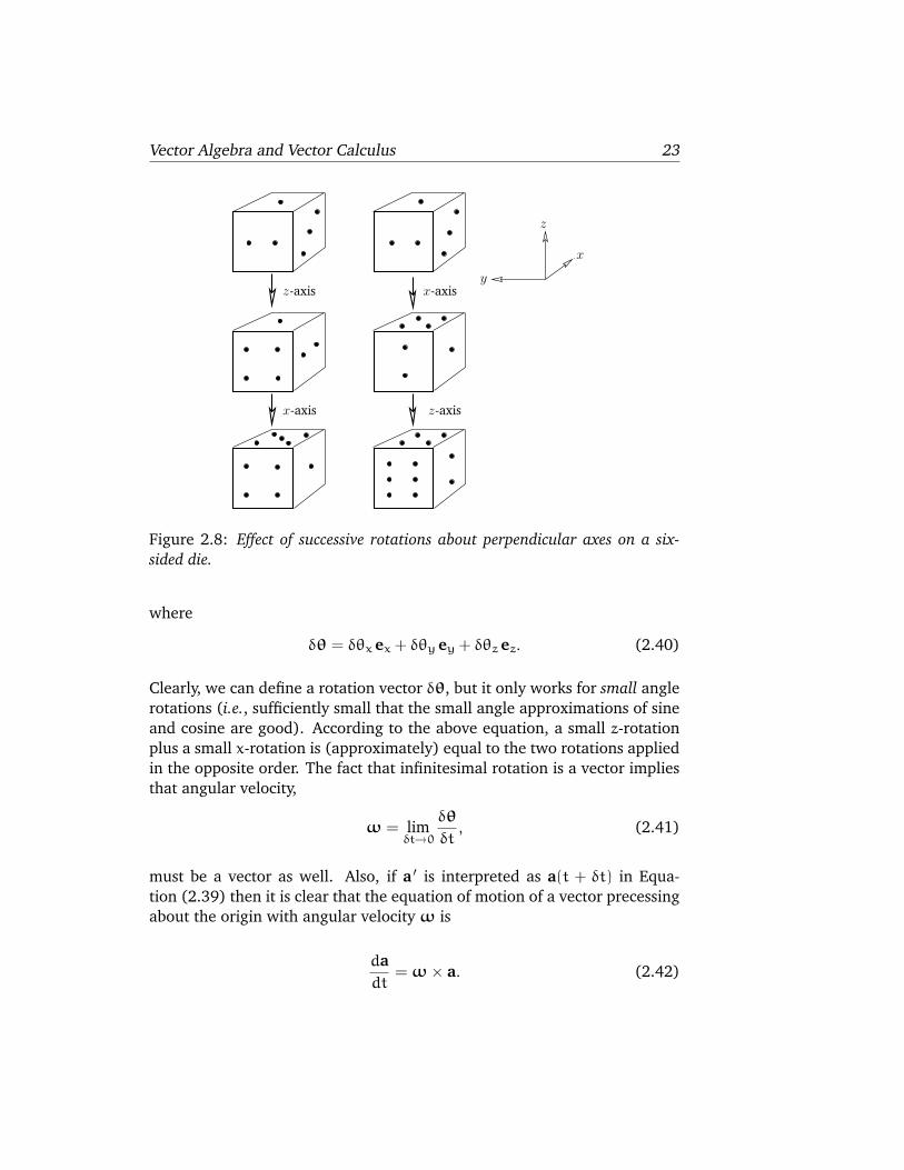
2.13 Exercises
1.1. Prove the trigonometric law of sines
sina
A=
sinb
B=
sin c
C
using vector methods. Here, a, b, and c are the three angles of a planetriangle, and A, B, and C the lengths of the corresponding opposite sides.
1.2. Demonstrate using vectors that the diagonals of a parallelogram bisect oneanother. In addition, show that if the diagonals of a quadrilateral bisect oneanother then it is a parallelogram.
1.3. From the inequality
a · b = |a| |b| cos θ ≤ |a| |b|
deduce the triangle inequality
|a + b| ≤ |a| + |b|.
1.4. Identify the following surfaces:
(a) |r| = a,
(b) r · n = b,
(c) r · n = c |r|,
(d) |r − (r · n) n| = d.
Here, r is the position vector, a, b, c, and d are positive constants, and n is afixed unit vector.
1.5. Let a, b, and c be coplanar vectors related via
α a + βb + γ c = 0,
where α, β, and γ are not all zero. Show that the condition for the pointswith position vectors u a, vb, and w c to be colinear is
α
u+β
v+γ
w= 0.
1.6. If p, q, and r are any vectors, demonstrate that a = q + λ r, b = r + µp, andc = p + νq are coplanar provided that λµν = −1, where λ, µ, and ν arescalars. Show that this condition is satisfied when a is perpendicular to p, bto q, and c to r.

Vector Algebra and Vector Calculus 37
1.7. The vectors a, b, and c are non-coplanar, and form a non-orthogonal vectorbase. The vectors A, B, and C, defined by
A =b × c
a · b × c,
plus cyclic permutations, are said to be reciprocal vectors. Show that
a = (B × C)/(A · B × C),
plus cyclic permutations.
1.8. In the notation of the previous question, demonstrate that the plane passingthrough points a/α, b/β, and c/γ is normal to the direction of the vector
h = αA + βB + γC.
In addition, show that the perpendicular distance of the plane from the originis |h|−1.
1.9. Find the gradients of the following scalar functions of the position vectorr = (x, y, z):
(a) k · r,
(b) |r|n,
(c) |r − k|−n,
(d) cos(k · r).
Here, k is a fixed vector.

38 NEWTONIAN DYNAMICS

Fundamental Concepts 39
3 Fundamental Concepts
3.1 Introduction
This chapter introduces the fundamental concepts which underlie all of
Newtonian Dynamics.
3.2 Fundamental Assumptions
Newtonian Dynamics is a mathematical model whose purpose is to pre-
dict the motions of the various objects which we encounter in the world
around us. The general principles of this theory were first enunciated by
Sir Isaac Newton in a work entitled Philosophiae Naturalis Principia Mathe-
matica (Mathematical Principles of Natural Philosophy). This work, which
was first published in 1687, is nowadays more commonly referred to as the
Principa.1
Up until the beginning of the 20th century, Newton’s theory of motion
was thought to constitute a complete description of all types of motion oc-
curring in the Universe. We now know that this is not the case. The modern
view is that Newton’s theory is only an approximation which is valid under
certain circumstances. The theory breaks down when the velocities of the
objects under investigation approach the speed of light in vacuum, and must
be modified in accordance with Einstein’s Special Theory of Relativity. The
theory also fails in regions of space which are sufficiently curved that the
propositions of Euclidean Geometry do not hold to a good approximation,
and must be augmented by Einstein’s General Theory of Relativity. Finally,
the theory breaks down on atomic and subatomic length-scales, and must be
replaced by Quantum Mechanics. In this book, we shall neglect relativistic
and quantum effects all together. It follows that we must restrict our inves-
tigations to the motions of large (compared to an atom), slow (compared to
the speed of light) objects moving in Euclidean space. Fortunately, virtually
all of the motions which we commonly observe in the world around us fall
into this category.
1An excellent discussion of the historical development of Newtonian Dynamics, as well
as the physical and philosophical assumptions which underpin this theory, is given in The
Discovery of Dynamics: A Study from a Machian Point of View of the Discovery and the Structure
of Dynamical Theories, J.B. Barbour (Oxford University Press, Oxford UK, 2001).

40 NEWTONIAN DYNAMICS
In the Principia, Newton very deliberately models his approach on that
taken in Euclid’s Elements. Indeed, Newton’s theory of motion has much in
common with a conventional axiomatic system such as Euclidean Geometry.
Like all axiomatic systems, Newtonian Dynamics starts from a set of terms
which are undefined within the system. In the this case, the fundamental
terms are mass, position, time, and force. It is taken for granted that we
understand what these terms mean, and, furthermore, that they correspond
to measurable quantities which can be ascribed to, or associated with, ob-
jects in the world around us. In particular, it is assumed that the ideas of
position in space, distance in space, and position as a function of time in
space, are correctly described by the Euclidean vector algebra and vector
calculus introduced in the previous chapter. The next component of an ax-
iomatic system is a set of axioms. These are a set of unproven propositions,
involving the undefined terms, from which all other propositions in the sys-
tem can be derived via logic and mathematical analysis. In the present case,
the axioms are called Newton’s laws of motion, and can only be justified via
experimental observation. Note, incidentally, that Newton’s laws, in their
primitive form, are only applicable to point objects. However, as we shall
see in Chapter 9, these laws can be applied to extended objects by treating
them as collections of point objects.
One difference between an axiomatic system and a physical theory is
that, in the latter case, even if a given prediction has been shown to follow
necessarily from the axioms of the theory, it is still incumbent upon us to
test the prediction against experimental observations. Lack of agreement
might indicate faulty experimental data, faulty application of the theory (for
instance, in the case of Newtonian Dynamics, there might be forces at work
which we have not identified), or, as a last resort, incorrectness of the theory.
Fortunately, Newtonian Dynamics has been found to give predictions which
are in excellent agreement with experimental observations in all situations
in which is expected to be valid.
In the following, it is assumed that we know how to set up a rigid Carte-
sian frame of reference, and how to measure the positions of point objects as
functions of time within that frame. It is also taken for granted that we have
some basic familiarity with the laws of mechanics, and standard mathemat-
ics up to, and including, calculus, as well as the vector analysis outlined in
Chapter 2.

Fundamental Concepts 41
3.3 Newton’s Laws of Motion
Newton’s laws of motion are as follows:
1. Every body continues in its state of rest, or uniform motion in a straight-
line, unless compelled to change that state by forces impressed upon
it.
2. The change of motion (i.e., momentum) of an object is proportional
to the force impressed upon it, and is made in the direction of the
straight-line in which the force is impressed.
3. To every action there is always opposed an equal reaction; or, the
mutual actions of two bodies upon each other are always equal and
directed to contrary parts.
3.4 Newton’s First Law of Motion
Newton’s first law of motion essentially states that a point object subject
to zero net external force moves in a straight-line with a constant speed
(i.e., it does not accelerate). However, this is only true in special frames of
reference called inertial frames. Indeed, we can think of Newton’s first law
as the definition of an inertial frame: i.e., an inertial frame of reference is
one in which a point object subject to zero net external force moves in a
straight-line with constant speed.
Suppose that we have found an inertial frame of reference. Let us set up
a Cartesian coordinate system in this frame. The motion of a point object
can now be specified by giving its position vector, r = (x, y, z), with respect
to the origin of the coordinate system, as a function of time, t. Consider
a second frame of reference moving with some constant velocity u with re-
spect to the first frame. Without loss of generality, we can suppose that the
Cartesian axes in the second frame are parallel to the corresponding axes in
the first frame, and that u = (u, 0, 0), and, finally, that the origins of the two
frames instantaneously coincide at t = 0—see Figure 3.1. Suppose that the
position vector of our point object is r ′ = (x ′, y ′, z ′) in the second frame
of reference. It is evident, from Figure 3.1, that at any given time, t, the
coordinates of the object in the two reference frames satisfy
x ′ = x− u t, (3.1)
y ′ = y, (3.2)
z ′ = z. (3.3)

42 NEWTONIAN DYNAMICS
u t
y y′
x x′
origin
Figure 3.1: A Galilean coordinate transformation.
This coordinate transformation is generally known as a Galilean transforma-
tion, after Galileo.
The instantaneous velocity of the object in our first reference frame is
given by v = dr/dt = (dx/dt, dy/dt, dz/dt), with an analogous expression
for the velocity, v ′, in the second frame. It follows from differentiation of
Equations (3.1)–(3.3) that the velocity components in the two frames satisfy
v ′x = vx− u, (3.4)
v ′y = vy, (3.5)
v ′z = vz. (3.6)
These equations can be written more succinctly as
v ′ = v − u. (3.7)
Finally, the instantaneous acceleration of the object in our first reference
frame is given by a = dv/dt = (dvx/dt, dvy/dt, dvz/dt), with an anal-
ogous expression for the acceleration, a ′, in the second frame. It follows
from differentiation of Equations (3.4)–(3.6) that the acceleration compo-
nents in the two frames satisfy
a ′x = ax, (3.8)
a ′y = ay, (3.9)
a ′z = az. (3.10)

Fundamental Concepts 43
These equations can be written more succinctly as
a ′ = a. (3.11)
According to Equations (3.7) and (3.11), if an object is moving in a
straight-line with constant speed in our original inertial frame (i.e., if a = 0)
then it also moves in a (different) straight-line with (a different) constant
speed in the second frame of reference (i.e., a ′ = 0). Hence, we conclude
that the second frame of reference is also an inertial frame.
A simple extension of the above argument allows us to conclude that
there are an infinite number of different inertial frames moving with con-
stant velocities with respect to one another.
But, what happens if the second frame of reference accelerates with re-
spect to the first? In this case, it is not hard to see that Equation (3.11)
generalizes to
a ′ = a −du
dt, (3.12)
where u(t) is the instantaneous velocity of the second frame with respect
to the first. According to the above formula, if an object is moving in a
straight-line with constant speed in the first frame (i.e., if a = 0) then it
does not move in a straight-line with constant speed in the second frame
(i.e., a ′ 6= 0). Hence, if the first frame is an inertial frame then the second is
not.
A simple extension of the above argument allows us to conclude that any
frame of reference which accelerates with respect to a given inertial frame
is not itself an inertial frame.
For most practical purposes, when studying the motions of objects close
to the Earth’s surface, a reference frame which is fixed with respect to this
surface is approximately inertial. However, if the trajectory of a projectile
within such a frame is measured to high precision then it will be found to de-
viate slightly from the predictions of Newtonian Dynamics—see Chapter 8.
This deviation is due to the fact that the Earth is rotating, and its surface is
therefore accelerating towards its axis of rotation. When studying the mo-
tions of objects in orbit around the Earth, a reference frame whose origin
is the center of the Earth and whose coordinate axes are fixed with respect
to distant stars is approximately inertial. However, if such orbits are mea-
sured to extremely high precision then they will again be found to deviate
very slightly from the predictions of Newtonian Dynamics. In this case, the
deviation is due to the Earth’s orbital motion about the Sun. When studying
the orbits of the Planets in the Solar System, a reference frame whose origin

44 NEWTONIAN DYNAMICS
is the center of the Sun and whose coordinate axes are fixed with respect to
distant stars is approximately inertial. In this case, any deviations of the or-
bits from the predictions of Newtonian Dynamics due to the orbital motion
of the Sun about the Galactic Center are far too small to be measurable. It
should be noted that it is impossible to identify an absolute inertial frame—
the best approximation to such a frame would be one in which the Cosmic
Microwave Background appears to be isotropic. However, for a given dy-
namical problem, it is always possible to identify an approximate inertial
frame. Furthermore, any deviations of such a frame from a true inertial
frame can be incorporated into the framework of Newtonian Dynamics via
the introduction of so-called fictitious forces—see Chapter 8.
3.5 Newton’s Second Law of Motion
Newton’s second law of motion essentially states that if a point object is
subject to an external force, f, then its equation of motion is given by
dp
dt= f, (3.13)
where the momentum, p, is the product of the object’s inertial mass, m,
and its velocity, v. If m is not a function of time then the above expression
reduces to the familiar equation
mdv
dt= f. (3.14)
Note that this equation is only valid in a inertial frame. Clearly, the inertial
mass of an object measures its reluctance to deviate from its preferred state
of uniform motion in a straight-line (in an inertial frame). Of course, the
above equation of motion can only be solved if we have an independent
expression for the force, f (i.e., a law of force). Let us suppose that this is
the case.
An important corollary of Newton’s second law is that force is a vector
quantity. This must be the case, since the law equates force to the product
of a scalar (mass) and a vector (acceleration). Note that acceleration is
obviously a vector because it is directly related to displacement, which is
the prototype of all vectors—see Chapter 2. One consequence of force being
a vector is that two forces, f1 and f2, both acting at a given point, have the
same effect as a single force, f = f1 + f2, acting at the same point, where
the summation is performed according to the laws of vector addition—see

Fundamental Concepts 45
Chapter 2. Likewise, a single force, f, acting at a given point, has the same
effect as two forces, f1 and f2, acting at the same point, provided that f1 +
f2 = f. This method of combining and splitting forces is known as the
resolution of forces, and lies at the heart of many calculations in Newtonian
Dynamics.
Taking the scalar product of Equation (3.14) with the velocity, v, we
obtain
m v·dv
dt=m
2
d(v · v)
dt=m
2
dv2
dt= f · v. (3.15)
This can be writtendK
dt= f · v. (3.16)
where
K =1
2mv2. (3.17)
The right-hand side of Equation (3.16) represents the rate at which the force
does work on the object: i.e., the rate at which the force transfers energy
to the object. The quantity K represents the energy the object possesses
by virtue of its motion. This type of energy is generally known as kinetic
energy. Thus, Equation (3.16) states that any work done on point object by
an external force goes to increase the object’s kinetic energy.
Suppose that, under the action of the force, f, our object moves from
point P at time t1 to point Q at time t2. The net change in the object’s
kinetic energy is obtained by integrating Equation (3.16):
∆K =
∫t2
t1
f · vdt =
∫Q
P
f · dr, (3.18)
since v = dr/dt. Here, dr is an element of the object’s path between points
P and Q.
As described in Section 2.12, there are basically two kinds of forces in
nature. Firstly, those for which line integrals of the type∫QP
f · dr depend on
the end points, but not on the path taken between these points. Secondly,
those for which line integrals of the type∫QP
f · dr depend both on the end
points, and the path taken between these points. The first kind of force is
termed conservative, whereas the second kind is termed non-conservative. It
was also demonstrated in Section 2.12 that if the line integral∫QP
f · dr is
path-independent then the force f can always be written as the gradient of a
scalar potential. In other words, all conservative forces satisfy
f = −∇U, (3.19)

46 NEWTONIAN DYNAMICS
for some scalar potential U(r). Note that
∫Q
P
∇U · dr = ∆U = U(Q) −U(P), (3.20)
irrespective of the path taken between P and Q. Hence, it follows from
Equation (3.18) that
∆K = −∆U (3.21)
for conservative forces. Another way of writing this is
E = K+U = constant. (3.22)
Of course, we recognize this as an energy conservation equation: E is the
object’s total energy, which is conserved; K is the energy the object has by
virtue of its motion, otherwise know as its kinetic energy; and U is the en-
ergy the object has by virtue of its position, otherwise known as its potential
energy. Note, however, that we can only write such energy conservation
equations for conservative forces (hence, the name). Gravity is a good ex-
ample of a conservative force. Non-conservative forces, on the other hand,
do not conserve energy. In general, this is because of some sort of fric-
tional energy loss which drains energy from the dynamical system whilst
it remains in motion. Note that potential energy is undefined to an arbi-
trary additive constant. In fact, it is only the difference in potential energy
between different points in space which is well-defined.
3.6 Newton’s Third Law of Motion
Consider a system ofNmutually interacting point objects. Let the ith object,
whose mass is mi, be located at vector displacement ri. Suppose that this
object exerts a force fji on the jth object. Likewise, suppose that the jth
object exerts a force fij on the ith object. Newton’s third law of motion
essentially states that these two forces are equal and opposite, irrespective
of their nature. In other words,
fij = −fji. (3.23)
One corollary of Newton’s third law is that an object cannot exert a force on
itself.
It should be noted that Newton’s third law implies action at a distance.
In other words, if the force that object i exerts on object j suddenly changes
then Newton’s third law demands that there must be an immediate change

Fundamental Concepts 47
in the force that object j exerts on object i. Moreover, this must be true
irrespective of the distance between the two objects. However, we now
known that Einstein’s Theory of Relativity forbids information from travel-
ing through the Universe faster than the velocity of light in vacuum. Hence,
action at a distance is also forbidden. In other words, if the force that ob-
ject i exerts on object j suddenly changes then there must be a time delay,
which is at least as long as it takes a light ray to propagate between the
two objects, before the force that object j exerts on object i can respond. Of
course, this means that Newton’s third law is not, strictly speaking, correct.
However, as long as we restrict our investigations to the motions of dynami-
cal systems on time-scales which are long compared to the time required for
light-rays to traverse these systems, Newton’s third law can be regarded as
being approximately correct.
In an inertial frame, Newton’s second law of motion applied to the ith
object yields
mid2ridt2
=
j6=i∑
j=1,N
fij. (3.24)
Note that the summation on the right-hand side of the above equation ex-
cludes the case j = i, since the ith object cannot exert a force on itself. Let
us now take the above equation and sum it over all objects. We obtain
∑
i=1,N
mid2ridt2
=
j6=i∑
i,j=1,N
fij. (3.25)
Consider the sum over forces on the right-hand side of the above equation.
Each element of this sum—fij, say—can be paired with another element—
fji, in this case—which is equal and opposite, according to Newton’s third
law. In other words, the elements of the sum all cancel out in pairs. Thus,
the net value of the sum is zero. It follows that the above equation can be
written
Md2rcm
dt2= 0, (3.26)
where M =∑Ni=1mi is the total mass. The quantity rcm is the vector dis-
placement of the center of mass of the system, which is an imaginary point
whose coordinates are the mass weighted averages of the coordinates of the
objects which constitute the system. Thus,
rcm =
∑Ni=1mi ri∑Ni=1mi
. (3.27)

48 NEWTONIAN DYNAMICS
According to Equation (3.26), the center of mass of the system moves in a
uniform straight-line, in accordance with Newton’s first law of motion, irre-
spective of the nature of the forces acting between the various components
of the system.
Now, if the center of mass moves in a uniform straight-line, then the
center of mass velocity,
drcm
dt=
∑Ni=1midri/dt∑Ni=1mi
, (3.28)
is a constant of the motion. However, the momentum of the ith object takes
the form pi = midri/dt. Hence, the total momentum of the system is
written
P =
N∑
i=1
midridt. (3.29)
A comparison of Equations (3.28) and (3.29) suggests that P is also a con-
stant of the motion. In other words, the total momentum of the system is
a conserved quantity, irrespective of the nature of the forces acting between
the various components of the system. This result (which only holds if there
is no net external force acting on the system) is a direct consequence of
Newton’s third law of motion.
Taking the vector product of Equation (3.24) with the position vector ri,
we obtain
mi ri×d2ridt2
=
j6=i∑
j=1,N
ri× fij. (3.30)
However, it is easily seen that
mi ri×d2ridt2
=d(mi ri× dri/dt)
dt=dlidt, (3.31)
where
li = mi ri×dridt
(3.32)
is the angular momentum of the ith particle about the origin of our coordi-
nate system. The total angular momentum of the system (about the origin)
takes the form
L =∑
i=1,N
li (3.33)

Fundamental Concepts 49
Hence, summing Equation (3.30) over all particles, we obtain
dL
dt=
i6=j∑
i,j=1,N
ri× fij. (3.34)
Consider the sum on the right-hand side of the above equation. A gen-
eral term, ri × fij, in this sum can always be paired with a matching term,
rj × fji, in which the indices have been swapped. Making use of Equa-
tion (3.23), the sum of a general matched pair can be written
ri× fij+ rj× fji = (ri− rj) × fij. (3.35)
Let us assume that the forces acting between the various components of the
system are central in nature, so that fij is parallel to ri− rj. In other words,
the force exerted on object j by object i either points directly toward, or
directly away from, object i, and vice versa. This is a reasonable assumption,
since most of the forces which we encounter in the world around us are of
this type (e.g., gravity). It follows that if the forces are central in nature then
the vector product on the right-hand side of the above expression is zero.
We conclude that
ri× fij+ rj× fji = 0, (3.36)
for all values of i and j. Thus, the sum on the right-hand side of Equa-
tion (3.34) is zero for any kind of central force. We are left with
dL
dt= 0. (3.37)
In other words, the total angular momentum of the system is a conserved
quantity, provided that the different components of the system interact via
central forces (and there is no net external torque acting on the system).
3.7 Exercises
1. Consider a system of N mutually interacting point objects. Let the ith objecthave mass mi and position vector ri. Suppose that the jth object exerts acentral force fij on the ith. In addition, let the ith object be subject to anexternal force Fi. Here, i and j take all possible values. Find expressionsfor the rate of change of the total linear momentum P and the total angularmomentum L of the system.

50 NEWTONIAN DYNAMICS
2. Consider an isolated system of N point objects interacting via gravity. Let themass and position vector of the ith object be mi and ri, respectively. Whatis the vector equation of motion of the ith object? Write expressions for thetotal kinetic energy, K, and potential energy, U, of the system. Demonstratefrom the equations of motion that K+U is a conserved quantity.
3. Consider a function of many variables f(x1, x2, · · · , xn). Such a functionwhich satisfies
f(t x1, t x2, · · · , t xn) = ta f(x1, x2, · · · , xn)
for all t > 0, and all values of the xi, is termed a homogenous function of
degree a. Prove the following theorem regarding homogeneous functions:
∑
i=1,n
xi∂f
∂xi= a f
4. Consider an isolated system of N point objects interacting via attractive cen-tral forces. Let the mass and position vector of the ith object be mi andri, respectively. Suppose that magnitude of the force exerted on object i byobject j is ki kj |ri−rj|
−n. Here, the ki measure some constant physical prop-erty of the particles (e.g., their electric charges). Write an expression for thetotal potential energy U of the system. Is this a homogenous function? If so,what is its degree? Write the equation of motion of the ith particle. Use themathematical theorem from the previous problem to demonstrate that
1
2
d2I
dt2= 2K+ (n− 1)U,
where I =∑i=1,Nmi r
2i , and K is the kinetic energy. This result is known
as the Virial theorem. Demonstrate that there are no bound steady-states forthe system when n ≥ 3.
5. Consider a system of N point particles. Let the ith particle have mass mi,electric charge qi, and position vector ri. Suppose that the charge to massratio, qi/mi, is the same for all particles. The system is placed in a uniformmagnetic field B. Write the equation of motion of the ith particle. You mayneglect any magnetic fields generated by motion of the particles. Demon-strate that the total momentum P of the system precesses about B at thefrequency Ω = qi B/mi. Demonstrate that L‖ +ΩI‖/2 is a constant of themotion. Here, L‖ is the total angular momentum of the system parallel to themagnetic field, and I‖ is the moment of inertia of the system about an axisparallel to B which passes through the origin.

One-Dimensional Motion 51
4 One-Dimensional Motion
4.1 Introduction
This chapter employs Newtonian Dynamics to investigate one-dimensional
motion. Particular attention is given to the various mathematical techniques
commonly used to analyze oscillatory motion.
4.2 Motion in a General One-Dimensional Potential
Consider a point particle of mass m moving in the x-direction, say, under
the action of some x-directed force f(x). Suppose that f(x) is a conservative
force: e.g., gravity. In this case, according to Equation (3.19), we can write
f(x) = −dU(x)
dx, (4.1)
where U(x) is the potential energy of the particle at position x.
Let the curve U(x) take the form shown in Figure 4.1. For instance, this
curve might represent the gravitational potential energy of a cyclist free-
wheeling in a hilly region. Observe that we have set the potential energy
at infinity to zero (which we are generally free to do, since potential en-
ergy is undefined to an arbitrary additive constant). This is a fairly common
convention. What can we deduce about the motion of the particle in this
potential?
Well, we know that the total energy, E—which is the sum of the kinetic
energy, K, and the potential energy, U—is a constant of the motion—see
Equation (3.22). Hence, we can write
K(x) = E−U(x). (4.2)
However, we also know that a kinetic energy can never be negative [since
K = (1/2)mv2, and neither m nor v2 can be negative]. Hence, the above
expression tells us that the particle’s motion is restricted to the region (or
regions) in which the potential energy curve U(x) falls below the value E.
This idea is illustrated in Figure 4.1. Suppose that the total energy of the
system is E0. It is clear, from the figure, that the particle is trapped inside one
or other of the two dips in the potential—these dips are generally referred
to as potential wells. Suppose that we now raise the energy to E1. In this

52 NEWTONIAN DYNAMICS
0
U→
x1x0 x2
E0
E1
x →
E2
Figure 4.1: A potential energy curve.
case, the particle is free to enter or leave each of the potential wells, but its
motion is still bounded to some extent, since it clearly cannot move off to
infinity. Finally, let us raise the energy to E2. Now the particle is unbounded:
i.e., it can move off to infinity. In conservative systems in which it makes
sense to adopt the convention that the potential energy at infinity is zero,
bounded systems are characterized by E < 0, whereas unbounded systems
are characterized by E > 0.
The above discussion suggests that the motion of an particle moving in
a potential generally becomes less bounded as the total energy E of the sys-
tem increases. Conversely, we would expect the motion to become more
bounded as E decreases. In fact, if the energy becomes sufficiently small
then it appears likely that the system will settle down in some equilibrium
state in which the particle is stationary. Let us try to identify any prospec-
tive equilibrium states in Figure 4.1. If the particle remains stationary then
it must be subject to zero force (otherwise it would accelerate). Hence,
according to Equation (4.1), an equilibrium state is characterized by
dU
dx= 0. (4.3)
In other words, a equilibrium state corresponds to either a maximum or a
minimum of the potential energy curve U(x). It can be seen that the U(x)
curve shown in Figure 4.1 has three associated equilibrium states located at
x = x0, x = x1, and x = x2.
Let us now make a distinction between stable equilibrium points and un-
stable equilibrium points. When the particle is slightly displaced from a sta-

One-Dimensional Motion 53
ble equilibrium point then the resultant force f acting on it must always be
such as to return it to this point. In other words, if x = x0 is an equilibrium
point then we requiredf
dx
∣
∣
∣
∣
x0
< 0 (4.4)
for stability: i.e., if the particle is displaced to the right, so that x − x0 > 0,
then the force must act to the left, so that f < 0, and vice versa. Likewise, if
df
dx
∣
∣
∣
∣
x0
> 0 (4.5)
then the equilibrium point x = x0 is unstable. It follows, from Equa-
tion (4.1), that stable equilibrium points are characterized by
d2U
dx2> 0. (4.6)
In other words, a stable equilibrium point corresponds to a minimum of
the potential energy curve U(x). Likewise, an unstable equilibrium point
corresponds to a maximum of the U(x) curve. Hence, we conclude that, in
Figure 4.1, x = x0 and x = x2 are stable equilibrium points, whereas x = x1is an unstable equilibrium point. Of course, this makes perfect sense if we
think of U(x) as a gravitational potential energy curve, so that U is directly
proportional to height. In this case, all we are saying is that it is easy to
confine a low energy mass at the bottom of a valley, but very difficult to
balance the same mass on the top of a hill (since any slight displacement of
the mass will cause it to fall down the hill). Note, finally, that if
dU
dx=d2U
dx2= 0 (4.7)
at any point (or in any region) then we have what is known as a neutral
equilibrium point. We can move the particle slightly away from such a point
and it will still remain in equilibrium (i.e., it will neither attempt to return
to its initial state, nor will it continue to move). A neutral equilibrium point
corresponds to a flat spot in a U(x) curve. See Figure 4.2.
The equation of motion of an particle moving in one dimension under
the action of a conservative force is, in principle, integrable. Since K =
(1/2)mv2, the energy conservation equation (4.2) can be rearranged to
give
v = ±(
2 [E−U(x)]
m
)1/2
, (4.8)

54 NEWTONIAN DYNAMICS
x →
U(x
)→
Stable Equilibrium Unstable Equilibrium Neutral Equilibrium
Figure 4.2: Different types of equilibrium point.
where the ± signs correspond to motion to the left and to the right, re-
spectively. However, since v = dx/dt, this expression can be integrated to
give
t = ±(
m
2E
)1/2 ∫x
x0
dx ′√
1−U(x ′)/E, (4.9)
where x(t = 0) = x0. For sufficiently simple potential functions, U(x), the
above equation can be solved to give x as a function of t. For instance, if
U = (1/2)k x2, x0 = 0, and the plus sign is chosen, then
t =
(
m
k
)1/2 ∫ (k/2E)1/2 x
0
dy√
1− y2=
(
m
k
)1/2
sin−1
(
[
k
2E
]1/2
x
)
, (4.10)
which can be inverted to give
x = a sin(ωt), (4.11)
where a =√
2 E/k andω =√
k/m. Note that the particle reverses direction
each time it reaches one of the so-called turning points (x = ±a) at which
U = E (and, so K = 0).
4.3 Velocity Dependent Forces
Consider a particle of mass m moving in one dimension under the action
of a force, f, which is a function of the particle’s speed, v, but not of its
displacement, x. Note that such a force is intrinsically non-conservative

One-Dimensional Motion 55
[since it clearly cannot be expressed as minus the gradient of some potential
function, U(x)]. Now, the particle’s equation of motion is written
mdv
dt= f(v). (4.12)
Integrating this equation, we obtain
∫v
v0
dv ′
f(v ′)=t
m, (4.13)
where v(t = 0) = v0. In principle, the above equation can be solved to give
v(t). The equation of motion is also written
mvdv
dx= f(v), (4.14)
since v = dx/dt. Integrating this equation, we obtain
∫v
v0
v ′ dv ′
f(v ′)=x− x0
m, (4.15)
where x(t = 0) = x0. In principle, the above equation can be solved to give
v(x).
Let us now consider a specific example. Suppose that an object of mass
m falls vertically under gravity. Let x be the height through which the ob-
ject has fallen since t = 0, at which time the object is assumed to be at
rest. It follows that x0 = v0 = 0. Suppose that, in addition to the force of
gravity, mg, where g is the gravitational acceleration, our object is subject
to a retarding air resistance force which is proportional to the square of its
instantaneous velocity. The object’s equation of motion is thus
mdv
dt= mg− c v2, (4.16)
where c > 0. This equation can be integrated to give
∫v
0
dv ′
1− (v ′/vt)2= g t, (4.17)
where vt = (mg/c)1/2. Making a change of variable, we obtain
∫v/vt
0
dy
1− y2=g
vtt. (4.18)

56 NEWTONIAN DYNAMICS
The left-hand side of the above equation is now a standard integral, which
can be solved to give
tanh−1
(
v
vt
)
=g t
vt, (4.19)
or
v = vt tanh
(
g t
vt
)
. (4.20)
Thus, when t≪ vt/g, we obtain the standard result v ≃ g t, since tanh x ≃ xfor x ≪ 1. However, when t ≫ vt/g, we get v ≃ vt, since tanh x ≃ 1 for
x ≫ 1. It follows that air resistance prevents the downward velocity of
our object from increasing indefinitely as it falls. Instead, at large times,
the velocity asymptotically approaches the so-called terminal velocity, vt (at
which the gravitational and air resistance forces balance).
The equation of motion of our falling object is also written
mvdv
dx= mg− c v2. (4.21)
This equation can be integrated to give
∫v
0
v ′ dv ′
1− (v ′/vt)2= g x. (4.22)
Making a change of variable, we obtain
∫ (v/vt)2
0
dy
1− y=x
xt, (4.23)
where xt = m/(2 c). The left-hand side of the above equation is now a
standard integral, which can be solved to give
− ln
[
1−
(
v
vt
)2]
=x
xt, (4.24)
or
v = vt
(
1− e−x/xt)1/2
. (4.25)
It follows that our object needs to fall a distance of order xt before it achieves
its terminal velocity.
Incidentally, it is quite easy to account for an air resistance force which
scales as the square of projectile velocity. Let us imaging that our projectile
is moving sufficiently rapidly that air does not have enough time to flow
around it, and is instead simply knocked out of the way. If our projectile has

One-Dimensional Motion 57
cross-sectional area A, perpendicular to the direction of its motion, and is
moving with speed v, then the mass of air that it knocks out of its way per
second is ρaAv, where ρa is the mass density of air. Suppose that the air
knocked out of the way is pushed in the direction of the projectile’s motion
with a speed of order v. It follows that the air gains momentum per unit time
ρaAv2 in the direction of the projectile’s motion. Hence, by Newton’s third
law, the projectile loses the same momentum per unit time in the direction
of its motion. In other words, the projectile is subject to a drag force of
magnitude
fdrag = CρaAv2 (4.26)
acting in the opposite direction to its motion. Here, C is an O(1) dimen-
sionless constant, known as the drag coefficient, which depends on the exact
shape of the projectile. Obviously, streamlined projectiles, such as arrows,
have small drag coefficients, whereas non-streamlined projectiles, such as
bricks, have large drag coefficients. From before, the terminal velocity of
our projectile is vt = (mg/c)1/2, where m is its mass, and c = CρaA. Writ-
ing m = Adρ, where d is the typical linear dimension of the projectile, and
ρ its mass density, we obtain
vt =
(
ρgd
ρaC
)1/2
. (4.27)
The above expression tells us that large, dense, streamlined projectiles (e.g.,
medicine balls) tend to have large terminal velocities, and small, rarefied,
non-streamlined projectiles (e.g., feathers) tend to have small terminal ve-
locities. Hence, the former type of projectile is relatively less affected by air
resistance than the latter.
4.4 Simple Harmonic Motion
Consider the motion of a point particle of massm which is slightly displaced
from a stable equilibrium point at x = 0. Suppose that the particle is moving
in the conservative force-field f(x). According to the analysis of Section 4.2,
in order for x = 0 to be a stable equilibrium point we require both
f(0) = 0, (4.28)
anddf(0)
dx< 0. (4.29)
58 NEWTONIAN DYNAMICS
Now, our particle obeys Newton’s second law of motion,
md2x
dt2= f(x). (4.30)
Let us assume that it always stays fairly close to its equilibrium point. In this
case, to a good approximation, we can represent f(x) via a truncated Taylor
expansion about this point. In other words,
f(x) ≃ f(0) +df(0)
dxx+ O(x2). (4.31)
However, according to (4.28) and (4.29), the above expression can be writ-
ten
f(x) ≃ −mω20 x, (4.32)
where df(0)/dx = −mω20 . Hence, we conclude that our particle satisfies
the following approximate equation of motion,
d2x
dt2+ω20 x ≃ 0, (4.33)
provided that it does not stray too far from its equilibrium point: i.e., pro-
vided |x| does not become too large.
Equation (4.33) is called the simple harmonic equation, and governs the
motion of all one-dimensional conservative systems which are slightly per-
turbed from some stable equilibrium state. The solution of Equation (4.33)
is well-known:
x(t) = a sin(ω0 t− φ0). (4.34)
The pattern of motion described by above expression, which is called simple
harmonic motion, is periodic in time, with repetition period T0 = 2π/ω0, and
oscillates between x = ±a. Here, a is called the amplitude of the motion.
The parameter φ0, known as the phase angle, simply shifts the pattern of
motion backward and forward in time. Figure 4.3 shows some examples of
simple harmonic motion. Here, φ0 = 0, +π/4, and −π/4 correspond to the
solid, short-dashed, and long-dashed curves, respectively.
Note that the frequency, ω0—and, hence, the period, T0—of simple har-
monic motion is determined by the parameters appearing in the simple har-
monic equation, (4.33). However, the amplitude, a, and the phase angle,
φ0, are the two integration constants of this second-order ordinary differen-
tial equation, and are, thus, determined by the initial conditions: i.e., by the
particle’s initial displacement and velocity.

One-Dimensional Motion 59
Figure 4.3: Simple harmonic motion.
Now, from Equations (4.1) and (4.32), the potential energy of our parti-
cle at position x is approximately
U(x) ≃ 1
2mω20 x
2. (4.35)
Hence, the total energy is written
E = K+U =1
2m
(
dx
dt
)2
+1
2mω20 x
2, (4.36)
giving
E =1
2mω20 a
2 cos2(ω0 t− φ0) +1
2mω20 a
2 sin2(ω0 t− φ0) =1
2mω20 a
2,
(4.37)
where use has been made of Equation (4.34), and the trigonometric identity
cos2θ + sin2θ ≡ 1. Note that the total energy is constant in time, as is to
be expected for a conservative system, and is proportional to the amplitude
squared of the motion.
4.5 Damped Oscillatory Motion
According to Equation (4.34), a one-dimensional conservative system which
is slightly perturbed from a stable equilibrium point (and then left alone)

60 NEWTONIAN DYNAMICS
oscillates about this point with a fixed frequency and a constant amplitude.
In other words, the oscillations never die away. This is not very realistic,
since we know that, in practice, if we slightly perturb a dynamical system
(such as a pendulum) from a stable equilibrium point then it will indeed
oscillate about this point, but these oscillations will eventually die away
due to frictional effects, which are present in virtually all real dynamical
systems. In order to model this process, we need to include some sort of
frictional drag force in our perturbed equation of motion, (4.33).
The most common model for a frictional drag force is one which is al-
ways directed in the opposite direction to the instantaneous velocity of the
object upon which it acts, and is directly proportional to the magnitude of
this velocity. Let us adopt this model. So, our drag force can be written
fdrag = −2mνdx
dt, (4.38)
where ν is a positive constant with the dimensions of frequency. Including
such a force in our perturbed equation of motion, (4.33), we obtain
d2x
dt2+ 2 ν
dx
dt+ω20 x = 0. (4.39)
Thus, the positive constant ν parameterizes the strength of the frictional
damping in our dynamical system.
Equation (4.39) is a linear second-order ordinary differential equation,
which we suspect possesses oscillatory solutions. There is a standard trick
for solving such an equation. We search for complex solutions of the form
x = a e−iωt, (4.40)
where the constants ω and a are both, in general, complex. Of course, the
physical solution is the real part of the above expression: i.e.,
x = |a| cos[arg(a) − Re(ω) t] e Im(ω)t. (4.41)
Clearly, the modulus and argument of the complex amplitude, a, determine
the amplitude (at t = 0) and phase of the oscillation, respectively, whereas
the real and imaginary parts of the complex frequency, ω, determine its
frequency and growth-rate, respectively. Note that this method of solution
is only appropriate for linear differential equations. Incidentally, the method
works because
Re[L(x)] ≡ L(Re[x]), (4.42)

One-Dimensional Motion 61
where x is a complex variable, and L some real linear differential operator
which acts on this variable. [A linear operator satisfies L(ax) = aL(x) for
all a and x, where a is a constant. The differential operator appearing in
Equation (4.39) is clearly of this type.]
Substituting Equation (4.40) into Equation (4.39), we obtain
a[
−ω2− i 2 νω+ω20
]
e−iωt = 0, (4.43)
which reduces to the following quadratic equation forω [since a exp(−iωt) 6=0]:
ω2+ i 2 νω−ω20 = 0. (4.44)
The solution to this equation is
ω± = −iν±√
ω20 − ν2. (4.45)
Thus, the most general physical solution to Equation (4.39) is
x(t) = Re[
a+ e−iω+ t+ a− e−iω− t]
, (4.46)
where a± are two arbitrary complex constants.
We can distinguish three different cases. In the first case, ν < ω0, and
the motion is said to be underdamped. The most general solution is written
x(t) = x0 e−νt cos(ωr t) +
(
v0+ νx0
ωr
)
e−νt sin(ωr t), (4.47)
where ωr =√
ω20 − ν2, x0 = x(0), and v0 = dx(0)/dt. It can be seen
that the solution oscillates at some real frequency, ωr, which is somewhat
less than the natural frequency of oscillation of the undamped system, ω0,
but also decays exponentially in time at a rate proportional to the damping
coefficient, ν.
In the second case, ν = ω0, and the motion is said to be critically
damped. The most general solution is written
x(t) = [x0 (1+ω0 t) + v0 t] e−ω0 t. (4.48)
It can be seen that the solution now decays without oscillating.
In the third case, ν > ω0, and the motion is said to be overdamped. The
most general solution is written
x(t) = −
(
v0+ ν−x0
ν+ − ν−
)
e−ν+ t+
(
v0+ ν+x0
ν+ − ν−
)
e−ν− t, (4.49)

62 NEWTONIAN DYNAMICS
Figure 4.4: Damped oscillatory motion.
where ν± = ν ±√
ν2−ω20 . It can be seen that the solution again decays
without oscillating, except there are now two independent decay rates. The
largest, ν+, is always greater than the critically damped decay rate, ω0,
whereas the smaller, ν−, is always less than this decay rate. This means
that, in general, the critically damped solution is more rapidly damped than
either the underdamped or overdamped solutions.
Figure 4.4 shows typical examples of underdamped (i.e., ν = ω0/4),
critically damped (i.e., ν = ω0), and overdamped (i.e., ν = 4ω0) solutions,
calculated with the initial conditions x0 = 1 and v0 = 0. Here, T0 = 2π/ω0.
The three solutions correspond to the solid, short-dashed, and long-dashed
curves, respectively.
4.6 Quality Factor
The total energy of a damped oscillator is the sum of its kinetic and potential
energies: i.e.,
E =1
2m
(
dx
dt
)2
+1
2mω20 x
2. (4.50)
Differentiating the above expression with respect to time, we obtain
dE
dt= m
dx
dt
d2x
dt2+mω20 x
dx
dt= m
dx
dt
(
d2x
dt2+ω20 x
)
. (4.51)

One-Dimensional Motion 63
It follows from Equation (4.39) that
dE
dt= −2mν
(
dx
dt
)2
. (4.52)
We conclude that the presence of damping causes the oscillator energy to
decrease monotonically in time, and, hence, causes the amplitude of the
oscillation to eventually become negligibly small [see Equation (4.37)].
The energy loss rate of a weakly damped (i.e., ν ≪ ω0) oscillator is
conveniently characterized in terms of a parameter, Q, which is known as
the quality factor. This parameter is defined to be 2π times the energy stored
in the oscillator, divided by the energy lost in a single oscillation period. If
the oscillator is weakly damped then the energy lost per period is relatively
small, and Q is therefore much larger than unity. Roughly speaking, Q is
the number of oscillations that the oscillator typically completes, after being
set in motion, before its amplitude decays to a negligible value. Let us find
an expression for Q.
Now, the most general solution for a weakly damped oscillator can be
written in the form [cf. Equation (4.47)]
x = x0 e−νt cos(ωr t− φ0), (4.53)
where x0 and φ0 are constants, and ωr =√
ω20 + ν2. It follows that
dx
dt= −x0ν e−νt cos(ωr t− φ0) − x0ωr e−νt sin(ωr t− φ0). (4.54)
Thus, making use of Equation (4.52), the energy lost during a single oscil-
lation period is
∆E = −
∫Tr
0
dE
dtdt (4.55)
= 2mνx20
∫Tr
0
e−2νt [ν cos(ωr t− φ0) +ωr sin(ωr t− φ0)]2dt,
where Tr = 2π/ωr. In the weakly damped limit, ν ≪ ωr, the exponential
factor is approximately unity in the interval t = 0 to t = Tr, so that
∆E ≃ 2mνx20ωr
∫2π
0
(
ν2 cos2θ+ 2 νωr cos θ sin θ+ω2r sin2θ)
dθ. (4.56)
Thus,
∆E ≃ 2πmνx20ωr
(ν2+ω2r ) = 2πmω20 x20
(
ν
ωr
)
, (4.57)

64 NEWTONIAN DYNAMICS
since cos2θ and sin2θ both have the average values 1/2 in the interval 0
to 2π, whereas cos θ sin θ has the average value 0. According to Equa-
tion (4.37), the energy stored in the oscillator (at t = 0) is
E =1
2mω20 x
20 . (4.58)
It follows that
Q = 2πE
∆E=ωr
2 ν≃ ω0
2 ν. (4.59)
4.7 Resonance
We have seen that when a one-dimensional dynamical system is slightly
perturbed from a stable equilibrium point (and then left alone), it eventually
returns to this point at a rate controlled by the amount of damping in the
system. Let us now suppose that the same system is subject to continuous
oscillatory constant amplitude external forcing at some fixed frequency, ω.
In this case, we would expect the system to eventually settle down to some
steady oscillatory pattern of motion with the same frequency as the external
forcing. Let us investigate the properties of this type of driven oscillation.
Suppose that our system is subject to an external force of the form
fext(t) = mω20 X1 cos(ωt). (4.60)
Here, X1 is the amplitude of the oscillation at which the external force
matches the restoring force, (4.32). Incorporating the above force into our
perturbed equation of motion, (4.39), we obtain
d2x
dt2+ 2 ν
dx
dt+ω20 x = ω20 X1 cos(ωt). (4.61)
Let us search for a solution of the form (4.40), and represent the right-hand
side of the above equation as ω20 X1 exp(−iωt). It is again understood that
the physical solutions are the real parts of these expressions. Note that ω is
now a real parameter. We obtain
a[
−ω2− i 2 νω+ω20
]
e−iωt = ω20 X1 e−iωt. (4.62)
Hence,
a =ω20 X1
ω20 −ω2− i 2 νω. (4.63)

One-Dimensional Motion 65
Figure 4.5: Resonance.
In general, a is a complex quantity. Thus, we can write
a = x1 e iφ1 , (4.64)
where x1 and φ1 are both real. It follows from Equations (4.40), (4.63),
and (4.64) that the physical solution takes the form
x(t) = x1 cos(ωt− φ1), (4.65)
where
x1 =ω20 X1
[
(ω20 −ω2)2+ 4 ν2ω2]1/2
, (4.66)
and
φ1 = tan−1
(
2 νω
ω20 −ω2
)
. (4.67)
We conclude that, in response to the applied sinusoidal force, (4.60), the
system executes a sinusoidal pattern of motion at the same frequency, with
fixed amplitude x1, and phase-lag φ1 (with respect to the external force).
Let us investigate the variation of x1 and φ1 with the forcing frequency,
ω. This is most easily done graphically. Figure 4.5 shows x1 and φ1 as func-
tions of ω for various values of ν/ω0. Here, ν/ω0 = 1, 1/2, 1/4, 1/8, and
1/16 correspond to the solid, dotted, short-dashed, long-dashed, and dot-
dashed curves, respectively. It can be seen that as the amount of damping
in the system is decreased, the amplitude of the response becomes progres-
sively more peaked at the natural frequency of oscillation of the system, ω0.

66 NEWTONIAN DYNAMICS
This effect is known as resonance, and ω0 is termed the resonant frequency.
Thus, a weakly damped system (i.e., ν≪ ω0) can be driven to large ampli-
tude by the application of a relatively small external force which oscillates
at a frequency close to the resonant frequency. Note that the response of the
system is in phase (i.e., φ1 ≃ 0) with the external driving force for driving
frequencies well below the resonant frequency, is in phase quadrature (i.e.,
φ1 = π/2) at the resonant frequency, and is in anti-phase (i.e., φ1 ≃ π) for
frequencies well above the resonant frequency.
According to Equation (4.66),
x1(ω = ω0)
x1(ω = 0)=ω0
2 ν= Q. (4.68)
In other words, the ratio of the driven amplitude at the resonant frequency
to that at a typical non-resonant frequency (for the same drive amplitude)
is of order the quality factor. Equation (4.66) also implies that, for a weakly
damped oscillator (ν≪ ω0),
x1(ω)
x1(ω = ω0)≃ ν
[(ω−ω0)2+ ν2]1/2, (4.69)
provided |ω − ω0| ≪ ω0. Hence, the width of the resonance peak (in
frequency) is ∆ω = 2 ν, where the edges of peak are defined as the points
at which the driven amplitude is reduced to 1/√2 of its maximum value. It
follows that the fractional width is
∆ω
ω0=2 ν
ω0=1
Q. (4.70)
We conclude that the height and width of the resonance peak of a weakly
damped (Q≫ 1) oscillator scale as Q and Q−1, respectively. Thus, the area
under the resonance curve stays approximately constant as Q varies.
4.8 Periodic Driving Forces
In the last section, we investigated the response of a one-dimensional dy-
namical system, close to a stable equilibrium point, to an external force
which varies as cos(ωt). Let us now examine the response of the same
system to a more complicated external force.
Consider a general external force which is periodic in time, with period
T . By analogy with Equation (4.60), we can write such a force as
fext(t) = mω20 X(t), (4.71)

One-Dimensional Motion 67
where
X(t+ T) = X(t) (4.72)
for all t.
It is convenient to represent X(t) as a Fourier series in time, so that
X(t) =
∞∑
n=0
Xn cos(nωt), (4.73)
where ω = 2π/T . By writing X(t) in this form, we automatically satisfy the
periodicity constraint (4.72). [Note that by choosing a cosine Fourier series
we are limited to even functions in t: i.e., X(−t) = X(t). Odd functions in
t can be represented by sine Fourier series, and mixed functions require a
combination of cosine and sine Fourier series.] The constant coefficients Xnare known as Fourier coefficients. But, how do we determine these coeffi-
cients for a given functional form, X(t)?
Well, it follows from the periodicity of the cosine function that
1
T
∫T
0
cos(nωt)dt = δn0, (4.74)
where δnn′ is unity if n = n ′, and zero otherwise, and is known as the
Kronecker delta function. Thus, integrating Equation (4.73) in t from t = 0
to t = T , and making use of Equation (4.74), we obtain
X0 =1
T
∫T
0
X(t)dt. (4.75)
It is also easily demonstrated that
2
T
∫T
0
cos(nωt) cos(n ′ωt)dt = δnn′ , (4.76)
provided n,n ′ > 0. Thus, multiplying Equation (4.73) by cos(nωt), inte-
grating in t from t = 0 to t = T , and making use of Equations (4.74) and
(4.76), we obtain
Xn =2
T
∫T
0
X(t) cos(nωt)dt (4.77)
for n > 0. Hence, we have now determined the Fourier coefficients of the
general periodic function X(t).

68 NEWTONIAN DYNAMICS
We can incorporate the periodic external force (4.71) into our perturbed
equation of motion by writing
d2x
dt2+ 2 ν
dx
dt+ω20 x = ω20
∞∑
n=0
Xne−inωt, (4.78)
where we are again using the convention that the physical solution corre-
sponds to the real part of the complex solution. Note that the above dif-
ferential equation is linear. This means that if xa(t) and xb(t) represent
two independent solutions to this equation then any linear combination of
xa(t) and xb(t) is also a solution. We can exploit the linearity of the above
equation to write the solution in the form
x(t) =
∞∑
n=0
Xnane−inωt, (4.79)
where the an are the complex amplitudes of the solutions to
d2x
dt2+ 2 ν
dx
dt+ω20 x = ω20 e−inωt. (4.80)
In other words, an is obtained by substituting x = an exp(−inωt) into the
above equation. Hence, it follows that
an =ω20
ω20 − n2ω2− i 2 νnω. (4.81)
Thus, the physical solution takes the form
x(t) =
∞∑
n=0
Xnxn cos(nωt− φn), (4.82)
where
an = xne iφn , (4.83)
and xn and φn are real parameters. It follows from Equation (4.81) that
xn =ω20
[
(ω20 − n2ω2)2+ 4 ν2n2ω2]1/2
, (4.84)
and
φn = tan−1
(
2 νnω
ω20 − n2ω2
)
. (4.85)

One-Dimensional Motion 69
Figure 4.6: Periodic forcing.
We have now fully determined the response of our dynamical system to a
general periodic driving force.
As an example, suppose that the external force periodically delivers a
brief kick to the system. For instance, let X(t) = A for 0 ≤ t ≤ T/10 and
9 T/10 < t < T , and X(t) = 0 otherwise (in the period 0 ≤ t ≤ T). It follows
from Equation (4.75) and (4.77) that, in this case,
X0 = 0.2A, (4.86)
and
Xn =2 sin(nπ/5)A
nπ, (4.87)
for n > 0. Obviously, to obtain an exact solution, we would have to include
every Fourier harmonic in Equation (4.82), which would be impractical.
However, we can obtain a fairly accurate approximate solution by truncating
the Fourier series (i.e., by neglecting all the terms with n > N, where N ≫1).
Figure 4.6 shows an example calculation in which the Fourier series is
truncated after 100 terms. The parameters used in this calculation are ω =
1.2ω0 and ν = 0.8ω0. The left panel shows the Fourier reconstruction
of the driving force, X(t). The glitches at the rising and falling edges of
the pulses are called Gibbs phenomena, and are an inevitable consequence
of attempting to represent a discontinuous periodic function as a Fourier
series. The right panel shows the Fourier reconstruction of the response,
x(t), of the dynamical system to the applied force.

70 NEWTONIAN DYNAMICS
4.9 Transients
We saw, in Section 4.7, that when a one-dimensional dynamical system,
close to a stable equilibrium point, is subject to a sinusoidal external force
of the form (4.60) then the equation of motion of the system is written
d2x
dt2+ 2 ν
dx
dt+ω20 x = ω20 X1 cos(ωt). (4.88)
We also found that the solution to this equation which oscillates in sympathy
with the applied force takes the form
x(t) = x1 cos(ωt− φ1), (4.89)
where x1 and φ1 are specified in Equations (4.66) and (4.67), respectively.
However, (4.89) is not the most general solution to Equation (4.88). It
should be clear that we can take the above solution and add to it any solu-
tion of Equation (4.88) calculated with the right-hand side set to zero, and
the result will also be a solution of Equation (4.88). Now, we investigated
the solutions to (4.88) with the right-hand set to zero in Section 4.5. In
the underdamped regime (ν < ω0), we found that the most general such
solution takes the form
x(t) = A e−νt cos(ωr t) + B e−νt sin(ωr t), (4.90)
where A and B are two arbitrary constants [they are in fact the integration
constants of the second-order ordinary differential equation (4.88)], and
ωr =√
ω20 − ν2. Thus, the most general solution to Equation (4.88) is
written
x(t) = A e−νt cos(ωr t) + B e−νt sin(ωr t) + x1 cos(ωt− φ1). (4.91)
The first two terms on the right-hand side of the above equation are called
transients, since they decay in time. The transients are determined by the
initial conditions. However, if we wait long enough after setting the system
into motion then the transients will always decay away, leaving the time-
asymptotic solution (4.89), which is independent of the initial conditions.
As an example, suppose that we set the system into motion at time t =
0 with the initial conditions x(0) = dx(0)/dt = 0. Setting x(0) = 0 in
Equation (4.91), we obtain
A = −x1 cosφ1. (4.92)

One-Dimensional Motion 71
Figure 4.7: Transients.
Moreover, setting dx(0)/dt = 0 in Equation (4.91), we get
B = −x1 (ν cosφ1+ω sinφ1)
ωr. (4.93)
Thus, we have now determined the constants A and B, and, hence, fully
specified the solution for t > 0. Figure 4.7 shows this solution (solid curve)
calculated for ω = 2ω0 and ν = 0.2ω0. Here, T0 = 2π/ω0. The associated
time-asymptotic solution (4.89) is also shown for the sake of comparison
(dashed curve). It can be seen that the full solution quickly converges to the
time-asymptotic solution.
4.10 Simple Pendulum
Consider a compact mass m suspended from a light inextensible string of
length l, such that the mass is free to swing from side to side in a vertical
plane, as shown in Figure 4.8. This setup is known as a simple pendulum.
Let θ be the angle subtended between the string and the downward vertical.
Obviously, the stable equilibrium state of the simple pendulum corresponds
to the situation in which the mass is stationary, and hangs vertically down
(i.e., θ = 0). The angular equation of motion of the pendulum is simply
Id2θ
dt2= τ, (4.94)

72 NEWTONIAN DYNAMICS
l
m g
pivot point
fixed support
θ
m
T
Figure 4.8: A simple pendulum.
where I is the moment of inertia of the mass, and τ is the torque acting
about the pivot point. For the case in hand, given that the mass is essentially
a point particle, and is situated a distance l from the axis of rotation (i.e.,
the pivot point), it is easily seen that I = ml2.
The two forces acting on the mass are the downward gravitational force,
mg, where g is the acceleration due to gravity, and the tension, T , in the
string. Note, however, that the tension makes no contribution to the torque,
since its line of action clearly passes through the pivot point. From sim-
ple trigonometry, the line of action of the gravitational force passes a dis-
tance l sin θ from the pivot point. Hence, the magnitude of the gravitational
torque ismg l sin θ. Moreover, the gravitational torque is a restoring torque:
i.e., if the mass is displaced slightly from its equilibrium state (i.e., θ = 0)
then the gravitational torque clearly acts to push the mass back toward that
state. Thus, we can write
τ = −mg l sin θ. (4.95)
Combining the previous two equations, we obtain the following angular
equation of motion of the pendulum:
ld2θ
dt2+ g sin θ = 0. (4.96)
Note that, unlike all of the other equations of motion which we have ex-
amined in this chapter, the above equation is nonlinear [since sin(aθ) 6=a sin θ, except when θ≪ 1].

One-Dimensional Motion 73
Let us assume, as usual, that the system does not stray very far from its
equilibrium state (θ = 0). If this is the case then we can make the small
angle approximation sin θ ≃ θ, and the above equation of motion simplifies
tod2θ
dt2+ω20 θ ≃ 0, (4.97)
where ω0 =√
g/l. Of course, this is just the simple harmonic equation.
Hence, we can immediately write the solution as
θ(t) = θ0 cos(ω0 t). (4.98)
We conclude that the pendulum swings back and forth at a fixed frequency,
ω0, which depends on l and g, but is independent of the amplitude, θ0, of
the motion.
Suppose, now, that we desire a more accurate solution of Equation (4.96).
One way in which we could achieve this would be to include more terms in
the small angle expansion of sin θ, which is
sin θ = θ−θ3
3!+θ5
5!+ · · · . (4.99)
For instance, keeping the first two terms in this expansion, Equation (4.96)
becomesd2θ
dt2+ω20 (θ− θ3/6) ≃ 0. (4.100)
By analogy with (4.98), let us try a trial solution of the form
θ(t) = ϑ0 cos(ωt). (4.101)
Substituting this into Equation (4.100), and making use of the trigonometric
identity
cos3u ≡ (3/4) cosu+ (1/4) cos(3u), (4.102)
we obtain
ϑ0
[
ω20 −ω2− (1/8)ω20 ϑ20
]
cos(ωt) − (1/24)ω20 ϑ30 cos(3ω t) ≃ 0.
(4.103)
It is evident that the above equation cannot be satisfied for all values of t,
except in the trivial case ϑ0 = 0. However, the form of this expression does
suggest a better trial solution, namely
θ(t) = ϑ0 cos(ωt) + αϑ30 cos(3ω t), (4.104)

74 NEWTONIAN DYNAMICS
where α is O(1). Substitution of this expression into Equation (4.100) yields
ϑ0
[
ω20 −ω2− (1/8)ω20 ϑ20
]
cos(ωt)+
ϑ30
[
αω20 − 9αω2− (1/24)ω20
]
cos(3ω t) + O(ϑ50) ≃ 0. (4.105)
We can only satisfy the above equation at all values of t, and for non-zero
ϑ0, by setting the two expressions in square brackets to zero. This yields
ω ≃ ω0√
1− (1/8) ϑ20 , (4.106)
and
α ≃ −ω20192
. (4.107)
Now, the amplitude of the motion is given by
θ0 = ϑ0+ αϑ30 = ϑ0−ω20192
ϑ30 . (4.108)
Hence, Equation (4.106) simplifies to
ω = ω0
[
1−θ2016
+ O(θ40)
]
. (4.109)
The above expression is only approximate, but it illustrates an important
point: i.e., that the frequency of oscillation of a simple pendulum is not, in
fact, amplitude independent. Indeed, the frequency goes down slightly as
the amplitude increases.
The above example illustrates how we might go about solving a nonlin-
ear equation of motion by means of an expansion in a small parameter (in
this case, the amplitude of the motion).
4.11 Exercises
1. A particle of mass m is constrained to move in one dimension such that itsinstantaneous displacement is x. The particle is released at rest from x = b,and is subject to a force of the form f(x) = −k x−2. Show that the timerequired for the particle to reach the origin is
π
(
mb3
8 k
)1/2
.

One-Dimensional Motion 75
2. A block of mass m slides along a horizontal surface which is lubricated withheavy oil such that the block suffers a viscous retarding force of the form
F = −c vn,
where c > 0 is a constant, and v is the block’s instantaneous velocity. If theinitial speed is v0 at time t = 0, find v and the displacement x as functions oftime t. Also find v as a function of x. Show that for n = 1/2 the block does
not travel further than 2mv3/2
0 /(3 c).
3. A particle is projected vertically upward in a constant gravitational field withan initial speed v0. Show that if there is a retarding force proportional tothe square of the speed then the speed of the particle when it returns to theinitial position is
v0 vt√
v 20 + v 2t
,
where vt is the terminal speed.
4. A particle of mass m moves (in one dimension) in a medium under the influ-ence of a retarding force of the form mk (v3 + a2 v), where v is the particlespeed, and k and a are positive constants. Show that for any value of theinitial speed the particle will never move a distance greater than π/(2 ka),and will only come to rest as t → ∞.
5. Two light springs have spring constants k1 and k2, respectively, and are usedin a vertical orientation to support an object of mass m. Show that the angu-lar frequency of oscillation is [(k1 + k2)/m]1/2 if the springs are in parallel,and [k1 k2/(k1 + k2)m]1/2 if the springs are in series.
6. A body of uniform cross-sectional area A and mass density ρ floats in a liquidof density ρ0 (where ρ < ρ0), and at equilibrium displaces a volume V. Showthat the period of small oscillations about the equilibrium position is
T = 2π
√
V
gA.
7. Show that the ratio of two successive maxima in the displacement of a dampedharmonic oscillator is constant.
8. If the amplitude of a damped harmonic oscillator decreases to 1/e of its initialvalue after n periods show that the ratio of the period of oscillation to theperiod of the same oscillator with no damping is
(
1+1
4π2 n2
)1/2
≃ 1+1
8π2 n2.

76 NEWTONIAN DYNAMICS
9. Consider a damped driven oscillator whose equation of motion is
d2x
dt2+ 2 ν
dx
dt+ω 2
0 x = F(t).
Let x = 0 and dx/dt = v0 at t = 0.
(a) Find the solution for t > 0 when F = sin(ωt).
(b) Find the solution for t > 0 when F = sin2(ωt).
10. Obtain the time asymptotic response of a damped linear oscillator of naturalfrequency ω0 and damping coefficient ν to a square-wave periodic forcingfunction of amplitude F0 = mω 20 X0 and frequency ω. Thus, F(t) = F0 for−π/2 < ωt < π/2, 3π/2 < ωt < 5π/2, etc., and F(t) = −F0 for π/2 < ωt <3π/2, 5π/2 < ωt < 7π/2, etc.

Multi-Dimensional Motion 77
5 Multi-Dimensional Motion
5.1 Introduction
This chapter employs Newtonian Dynamics to investigate various aspects of
multi-dimensional motion.
5.2 Motion in a Two-Dimensional Harmonic Potential
Consider a particle of mass m moving in the two-dimensional harmonic
potential
U(x, y) =1
2k r2, (5.1)
where r =√
x2+ y2, and k > 0. It follows that the particle is subject to a
force,
f = −∇U = −k (x, y) = −k r, (5.2)
which always points towards the origin, and whose magnitude increases
linearly with increasing distance from the origin. According to Newton’s
second law, the equation of motion of the particle is
md2r
dt2= f = −k r. (5.3)
When written in component form, the above equation reduces to
d2x
dt2= −ω20 x, (5.4)
d2y
dt2= −ω20 y, (5.5)
where ω0 =√
k/m.
Since Equations (5.4) and (5.5) are both simple harmonic equations, we
can immediately write their general solutions:
x = A cos(ω0 t− φ1), (5.6)
y = B cos(ω0 t− φ2). (5.7)

78 NEWTONIAN DYNAMICS
Here, A, B, φ1, and φ2 are arbitrary constants of integration. We can sim-
plify the above equations slightly by shifting the origin of time (which is,
after all, arbitrary): i.e.,
t → t ′ + φ1/ω0. (5.8)
Hence, we obtain
x = A cos(ω0 t′), (5.9)
y = B cos(ω0 t′ − ∆), (5.10)
where ∆ = φ2 − φ1. Note that the motion is clearly periodic in time, with
period T = 2 π/ω0. Thus, the particle must trace out some closed trajectory
in the x-y plane. The question, now, is what does this trajectory look like as
a function of the relative phase-shift, ∆, between the oscillations in the x-
and y-directions?
Using standard trigonometry, we can write Equation (5.10) in the form
y = B[
cos(ω0 t′) cos∆+ sin(ω0 t
′) sin∆]
. (5.11)
Hence, using Equation (5.9), we obtain
(
y
B−x
Acos∆
)2
= sin2(ω0 t′) sin2∆ =
(
1−x2
A2
)
sin2∆, (5.12)
which simplifies to give
x2
A2− 2
x y
ABcos∆+
y2
B2= sin2∆. (5.13)
Unfortunately, the above equation is not immediately recognizable as being
the equation of any particular geometric curve: e.g., a circle, an ellipse, or a
parabola, etc.
Perhaps our problem is that we are using the wrong coordinates. Sup-
pose that we rotate our coordinate axes about the z-axis by an angle θ, as
illustrated in Figure 2.3. According to Equations (2.8) and (2.9), our old
coordinates (x, y) are related to our new coordinates (x ′, y ′) via
x = x ′ cosθ− y ′ sin θ, (5.14)
y = x ′ sin θ+ y ′ cos θ. (5.15)

Multi-Dimensional Motion 79
Let us see whether Equation (5.13) takes a simpler form when expressed in
terms of our new coordinates. Equations (5.13)–(5.15) yield
x ′2[
cos2θ
A2−2 cosθ sin θ cos∆
AB+
sin2θ
B2
]
+y ′2[
sin2θ
A2+2 cos θ sin θ cos∆
AB+
cos2θ
B2
]
(5.16)
+x ′ y ′[
−2 sin θ cos θ
A2+2 (sin2θ− cos2θ) cos∆
AB+2 cos θ sin θ
B2
]
= sin2∆.
We can simplify the above equation by setting the term involving x ′ y ′ to
zero. Hence,
−sin(2 θ)
A2−2 cos(2 θ) cos∆
AB+
sin(2 θ)
B2= 0, (5.17)
where we have made use of some simple trigonometric identities. Thus, the
x ′ y ′ term disappears when θ takes the special value
θ =1
2tan−1
(
2AB cos∆
A2− B2
)
. (5.18)
In this case, Equation (5.16) reduces to
x ′2
a2+y ′2
b2= 1, (5.19)
where
1
a2=
1
sin2∆
[
cos2θ
A2−2 cos θ sin θ cos∆
AB+
sin2θ
B2
]
, (5.20)
1
b2=
1
sin2∆
[
sin2θ
A2+2 cos θ sin θ cos∆
AB+
cos2θ
B2
]
. (5.21)
Of course, we immediately recognize Equation (5.19) as the equation of
an ellipse, centered on the origin, whose major and minor axes are aligned
along the x ′- and y ′-axes, and whose major and minor radii are a and b,
respectively (assuming that a > b).
We conclude that, in general, a particle of mass m moving in the two-
dimensional harmonic potential (5.1) executes a closed elliptical orbit (which
is not necessarily aligned along the x- and y-axes), centered on the origin,
with period T = 2 π/ω0, where ω0 =√
k/m.

80 NEWTONIAN DYNAMICS
(a) (b)
(c) (d)
Figure 5.1: Trajectories in a two-dimensional harmonic oscillator potential.
Figure 5.1 shows some example trajectories calculated for A = 2, B =
1, and the following values of the phase difference, ∆: (a) ∆ = 0; (b)
∆ = π/4; (c) ∆ = π/2; (d) ∆ = 3π/4. Note that when ∆ = 0 the trajectory
degenerates into a straight-line (which can be thought of as an ellipse whose
minor radius is zero).
Perhaps, the main lesson to be learned from the above study of two-
dimensional motion in a harmonic potential is that comparatively simple
patterns of motion can be made to look complicated when written in terms
of ill-chosen coordinates.
5.3 Projectile Motion with Air Resistance
Suppose that a projectile of mass m is launched, at t = 0, from ground
level (in a horizontal plane), making an angle θ to the horizontal. Suppose,
further, that, in addition to the force of gravity, the projectile is subject to
an air resistance force which acts in the opposite direction to its instanta-
neous direction of motion, and whose magnitude is directly proportional to
its instantaneous speed. This is not a particularly accurate model of the
drag force due to air resistance (the magnitude of the drag force is typically

Multi-Dimensional Motion 81
proportion to the square of the speed—see Section 4.3), but it does lead to
tractable equations of motion. Hence, by using this model we can, at least,
get some idea of how air resistance modifies projectile trajectories.
Let us adopt a Cartesian coordinate system whose origin coincides with
the launch point, and whose z-axis points vertically upward. Let the initial
velocity of the projectile lie in the x-z plane. Note that, since neither gravity
nor the drag force causes the projectile to move out of the x-z plane, we can
effectively ignore the y coordinate in this problem.
The equation of motion of our projectile is written
mdv
dt= m g − c v, (5.22)
where v = (vx, vz) is the projectile velocity, g = (0,−g) the acceleration due
to gravity, and c a positive constant. In component form, the above equation
becomes
dvx
dt= −g
vx
vt, (5.23)
dvz
dt= −g
(
1+vz
vt
)
. (5.24)
Here, vt = mg/c is the terminal velocity: i.e., the velocity at which the
drag force balances the gravitational force (for a projectile falling vertically
downward).
Integrating Equation (5.23), we obtain∫v
vx 0
dvx
vx= −
g
vtt, (5.25)
where vx0 = v0 cos θ is the x-component of the launch velocity. Hence,
ln
(
vx
vx0
)
= −g
vtt, (5.26)
or
vx = v0 cosθ e−gt/vt . (5.27)
It is clear, from the above equation, that air drag causes the projectile’s hor-
izontal velocity, which would otherwise be constant, to decay exponentially
on a time-scale of order vt/g.
Integrating Equation (5.24), we get∫vz
vz 0
dvz
vt+ vz= −
g
vtt, (5.28)

82 NEWTONIAN DYNAMICS
where vz0 = v0 sin θ is the z-component of the launch velocity. Hence,
ln
(
vt+ vz
vt+ vz0
)
= −g
vtt, (5.29)
or
vz = v0 sin θ e−gt/vt − vt
(
1− e−gt/vt)
. (5.30)
It thus follows, from Equations (5.27) and (5.30), that if the projectile stays
in the air much longer than a time of order vt/g then it ends up falling
vertically downward at the terminal velocity, vt, irrespective of its initial
launch angle.
Integration of (5.27) yields
x =v0 vt cos θ
g
(
1− e−gt/vt)
. (5.31)
In the limit t≪ vt/g, the above equation reduces to
x = v0 cos θ t, (5.32)
which is the standard result in the absence of air drag. In the opposite limit,
t≫ vt/g, we get
x =v0 vt cos θ
g. (5.33)
The above expression clearly sets an effective upper limit on how far the
projectile can travel in the horizontal direction.
Integration of (5.30) gives
z =vt
g(v0 sin θ+ vt)
(
1− e−gt/vt)
− vt t. (5.34)
In the limit t≪ vt/g, this equation reduces to
z = v0 sin θ t−g
2t2, (5.35)
which is the standard result in the absence of air drag. In the opposite limit,
t≫ vt/g, we get
z =vt
g(v0 sin θ+ vt) − vt t. (5.36)
Incidentally, the above analysis implies that air resistance only starts to have
an appreciable effect on the trajectory after the projectile has been in the air
a time of order vt/g.

Multi-Dimensional Motion 83
It is clear, from the previous two equations, that the time of flight of the
projectile (i.e., the time at which z = 0, excluding the trivial result t = 0) is
tf =2 v0 sin θ
g(5.37)
when t≪ vt/g, which implies that v0 sin θ≪ vt, and
tf =v0 sin θ
g(5.38)
when t ≫ vt/g, which implies that v0 sin θ ≫ vt. It thus follows, from
Equations (5.32) and (5.33), that the horizontal range [i.e., x(tf)] of the
projectile is
R =v20 sin(2 θ)
g(5.39)
when v0 sin θ≪ vt, and
R =v0 vt cos θ
g(5.40)
when v0 sin θ≫ vt. Equation (5.39) is, of course, the standard result with-
out air resistance. This result implies that, in the absence of air resistance,
the maximum horizontal range, v20/g, is achieved when the launch angle
θ takes the value 45. On the other hand, Equation (5.40) implies that, in
the presence of air resistance, the maximum horizontal range, v0 vt/g, is
achieved when θ is made as small as possible. However, θ cannot be made
too small, since expression (5.40) is only valid when v0 sin θ ≫ vt. In fact,
assuming that v0≫ vt, the maximum horizontal range, v0 vt/g, is achieved
when θ ∼ vt/v0 ≪ 1. We thus conclude that if air resistance is significant
then it causes the horizontal range of the projectile to scale linearly, rather
than quadratically, with the launch velocity, v0. Moreover, the maximum
horizontal range is achieved with a launch angle which is much shallower
than the standard result, 45.Figure 5.2 shows some example trajectories calculated, from the above
model, with the same launch angle, 45, but with different values of the
ratio v0/vt. Here, X = x/(v20/g) and Z = z/(v20/g). The solid, short-dashed,
long-dashed, and dot-dashed curves correspond to v0/vt = 0, 1, 2, and 4,
respectively. It can be seen that as the air resistance strength increases (i.e.,
as v0/vt increases), the range of the projectile decreases. Furthermore, there
is always an initial time interval during which the trajectory is identical to
that calculated in the absence of air resistance (i.e., v0/vt = 0). Finally, in
the presence of air resistance, the projectile tends to fall more steeply than

84 NEWTONIAN DYNAMICS
Figure 5.2: Projectile trajectories in the presence of air resistance.
it rises. Indeed, in the presence of strong air resistance (i.e., v0/vt = 4), the
projectile falls almost vertically.
5.4 Charged Particle Motion in Electric and Magnetic Fields
Consider a particle of mass m and electric charge q moving in the uniform
electric and magnetic fields, E and B. Suppose that the fields are “crossed”
(i.e., perpendicular to one another), so that E · B = 0.
The force acting on the particle is given by the familiar Lorentz law:
f = q (E + v × B) , (5.41)
where v is the particle’s instantaneous velocity. Hence, from Newton’s sec-
ond law, the particle’s equation of motion can be written
mdv
dt= q (E + v × B) . (5.42)
It turns out that we can eliminate the electric field from the above equa-
tion by transforming to a different inertial frame. Thus, writing
v =E × B
B2+ v ′, (5.43)

Multi-Dimensional Motion 85
Equation (5.42) reduces to
mdv ′
dt= q v ′ × B, (5.44)
where we have made use of a standard vector identity (see Section 2.7),
as well as the fact that E · B = 0. Hence, we conclude that the addition of
an electric field perpendicular to a given magnetic field simply causes the
particle to drift perpendicular to both the electric and magnetic field with
the fixed velocity
vEB =E × B
B2, (5.45)
irrespective of its charge or mass, It follows that the electric field has no
effect on the particle’s motion in a frame of reference which is co-moving
with the so-called E-cross-B velocity given above.
Let us suppose that the magnetic field is directed along the z-axis. As we
have just seen, in the E×B frame, the particle’s equation of motion reduces
to Equation (5.44), which can be written:
dv ′xdt
= Ωv ′y, (5.46)
dv ′ydt
= −Ωv ′x, (5.47)
v ′z = 0. (5.48)
Here,
Ω =qB
m(5.49)
is the so-called cyclotron frequency. Equations (5.46)–(5.48) can be inte-
grated to give
v ′x = v⊥ sin(Ωt), (5.50)
v ′y = v⊥ cos(Ωt) (5.51)
v ′z = v‖, (5.52)
where we have judiciously chosen the origin of time so as to eliminate any
phase offset in the arguments of the above trigonometrical functions. Ac-
cording to Equations (5.50)–(5.52), in the E×B frame, our charged particle
gyrates at the cyclotron frequency in the plane perpendicular to the mag-
netic field with some fixed speed v⊥, and drifts parallel to the magnetic

86 NEWTONIAN DYNAMICS
field with some fixed speed v‖. The fact that the cyclotron frequency is pos-
itive for positively charged particles, and negative for negatively charged
particles, just means that oppositely charged particles gyrate in opposite di-
rections in the plane perpendicular to the magnetic field.
Equations (5.50)–(5.52) can be integrated to give
x ′ = −ρ cos(Ωt), (5.53)
y ′ = ρ sin(Ωt) (5.54)
z ′ = v‖ t, (5.55)
where we have judiciously chosen the origin of our coordinate system so as
to eliminate any constant offsets in the above equations. Here,
ρ =v⊥Ω
(5.56)
is called the Larmor radius. Equations (5.53)–(5.55) are the equations of a
spiral of radius ρ, aligned along the direction of the magnetic field (i.e., the
z-direction).
ρB
Figure 5.3: The spiral trajectory of a negatively charged particle in a magnetic
field.
We conclude that the general motion of a charged particle in crossed
electric and magnetic field is a combination of E × B drift [see Equation
(5.45)] and spiral motion aligned along the direction of the magnetic field—
see Figure 5.3. Particles drift parallel to the magnetic field with constant
speeds, and gyrate at the cyclotron frequency in the plane perpendicular to
the magnetic field with constant speeds. Oppositely charged particles gyrate
in opposite directions.
5.5 Exercises
1. An electron of mass m and charge −e moves in a uniform y-directed electricfield of magnitude E, and a uniform z-directed magnetic field of magnitude

Multi-Dimensional Motion 87
B. The electron is situated at the origin at t = 0 with an initial x-directedvelocity of magnitude v0. Show that the electron traces out a cycloid of thegeneral form
x = a sin(ωt) + b t,
y = c [1− cos(ωt)],
z = 0.
Find the values of a, b, c, and ω, and sketch the electron’s trajectory in thex-y plane when v0 < E/B, E/B < v0 < 2E/B, and v0 > 2E/B.
2. A particle of mass m and charge q moves in the x-y plane under the in-fluence of a constant amplitude rotating electric field which is such thatEx = E0 cos(ωt) and Ey = E0 sin(ωt). The particle starts at rest fromthe origin. Determine its subsequent motion. What shape is the particle’strajectory?
3. A particle of massm slides on a frictionless surface whose height is a functionof x only: i.e., z = z(x). The function z(x) is specified by the parametricequations
x = A [2φ+ sin(2φ)],
z = A [1− cos(2φ)],
where φ is the parameter. Show that the total energy of the particle can bewritten
E =m
2
(
ds
dt
)2
+1
2
mg
4As2,
where s = 4A sinφ. Deduce that the particle undergoes periodic motionwhose frequency is amplitude independent (even when the amplitude islarge). Demonstrate that the frequency of the motion is given by 4π (A/g)1/2.

88 NEWTONIAN DYNAMICS

Planetary Motion 89
6 Planetary Motion
6.1 Introduction
Newtonian Dynamics was initially developed in order to account for the
motion of the Planets around the Sun. Let us now investigate this problem.
6.2 Kepler’s Laws
As is well-known, Johannes Kepler was the first astronomer to correctly
describe planetary motion in the Solar System (in works published between
1609 and 1619). The motion of the Planets is summed up in three simple
laws:
1. The planetary orbits are all ellipses which are confocal with the Sun
(i.e., the Sun lies at one of the focii of each ellipse).
2. The radius vectors connecting each planet to the Sun sweep out equal
areas in equal time intervals.
3. The squares of the orbital periods of the planets are proportional to
the cubes of their orbital major radii.
Let us now see if we can derive Kepler’s laws from Newton’s laws of motion.
6.3 Newtonian Gravity
The force which maintains the Planets in orbit around the Sun is called grav-
ity, and was first correctly described by Isaac Newton (in 1687). According
to Newton, any two point mass objects (or spherically symmetric objects of
finite extent) exert a force of attraction on one another. This force points
along the line of centers joining the objects, is directly proportional to the
product of the objects’ masses, and inversely proportional to the square of
the distance between them. Suppose that the first object is the Sun, which
is of mass M, and is located at the origin of our coordinate system. Let the
second object be some planet, of massm, which is located at position vector
r. The gravitational force exerted on the planet by the Sun is thus written
f = −GMm
r3r. (6.1)

90 NEWTONIAN DYNAMICS
The constant of proportionality, G, is called the gravitational constant, and
takes the value
G = 6.67300× 10⁻¹¹m3 kg−1 s−2. (6.2)
An equal and opposite force to (6.1) acts on the Sun. However, we shall
assume that the Sun is so much more massive than the planet in question
that this force does not cause the Sun’s position to shift appreciably. Hence,
the Sun always remains at the origin of our coordinate system. Likewise,
we shall neglect the gravitational forces exerted on our planet by the other
planets in the Solar System compared to the much larger gravitational force
exerted by the Sun.
Incidentally, there is something rather curious about Equation (6.1). Ac-
cording to this law, the gravitational force acting on an object is directly pro-
portional to its inertial mass. But why should inertia be related to the force
of gravity? After all, inertia measures the reluctance of a given body to devi-
ate from its preferred state of uniform motion in a straight-line, in response
to some external force. What has this got to do with gravitational attraction?
This question perplexed physicists for many years, and was only answered
when Albert Einstein published his General Theory of Relativity in 1916. Ac-
cording to Einstein, inertial mass acts as a sort of gravitational charge since
it impossible to distinguish an acceleration generated by a gravitational field
from an apparent acceleration generated by being in a non-inertial frame.
The assumption that these two types of acceleration are indistinguishable
leads directly to all of the strange predictions of General Relativity: e.g.,
clocks in different gravitational potentials run at different rates, mass bends
space, etc.
According to Equation (6.1), and Newton’s second law, the equation of
motion of our planet takes the form
d2r
dt2= −
GM
r3r. (6.3)
Note that the planetary mass,m, has canceled out on both sides of the above
equation.
6.4 Conservation Laws
Now gravity is a conservative force. Hence, the gravitational force (6.1) can
be written (see Section 3.5)
f = −∇U, (6.4)

Planetary Motion 91
where the potential energy, U(r), of our planet in the Sun’s gravitational
field takes the form
U(r) = −GMm
r. (6.5)
It follows that the total energy of our planet is a conserved quantity—see
Section 3.5. In other words,
E =v2
2−GM
r(6.6)
is constant in time. Here, E is actually the planet’s total energy per unit
mass, and v = dr/dt.
Gravity is also a central force. Hence, the angular momentum of our
planet is a conserved quantity—see Section 3.6. In other words,
h = r × v, (6.7)
which is actually the planet’s angular momentum per unit mass, is constant
in time. Taking the scalar product of the above equation with r, we obtain
h · r = 0. (6.8)
This is the equation of a plane which passes through the origin, and whose
normal is parallel to h. Since h is a constant vector, it always points in the
same direction. We, therefore, conclude that the motion of our planet is two-
dimensional in nature: i.e., it is confined to some fixed plane which passes
through the origin. Without loss of generality, we can let this plane coincide
with the x-y plane.
6.5 Plane Polar Coordinates
We can determine the instantaneous position of our planet in the x-y plane
in terms of standard Cartesian coordinates, (x, y), or plane polar coordi-
nates, (r, θ), as illustrated in Figure 6.1. It is helpful to define two unit
vectors, er ≡ r/r and eθ ≡ ez × er, at the instantaneous position of the
planet. The first always points radially away from the origin, whereas the
second is normal to the first, in the direction of increasing θ. As is easily
demonstrated, the Cartesian components of er and eθ are
er = (cos θ, sin θ), (6.9)
eθ = (− sin θ, cos θ), (6.10)

92 NEWTONIAN DYNAMICS
eθ
θ
y
x
r
er
Figure 6.1: Plane polar coordinates.
y
b
ax
Figure 6.2: An ellipse.
Planetary Motion 93
respectively.
We can write the position vector of our planet as
r = r er. (6.11)
Thus, the planet’s velocity becomes
v =dr
dt= r er+ r er, (6.12)
where ˙ is shorthand for d/dt. Note that er has a non-zero time-derivative
(unlike a Cartesian unit vector) because its direction changes as the planet
moves around. As is easily demonstrated, from differentiating Equation (6.9)
with respect to time,
er = θ (− sin θ, cos θ) = θ eθ. (6.13)
Thus,
v = r er+ r θ eθ. (6.14)
Now, the planet’s acceleration is written
a =dv
dt=d2r
dt2= r er+ r er+ (r θ+ r θ) eθ+ r θ eθ. (6.15)
Again, eθ has a non-zero time-derivative because its direction changes as
the planet moves around. Differentiation of Equation (6.10) with respect to
time yields
eθ = θ (− cosθ, − sin θ) = −θ er. (6.16)
Hence,
a = (r− r θ2) er+ (r θ+ 2 r θ) eθ. (6.17)
It follows that the equation of motion of our planet, (6.3), can be written
a = (r− r θ2) er+ (r θ+ 2 r θ) eθ = −GM
r2er. (6.18)
Since er and eθ are mutually orthogonal, we can separately equate the co-
efficients of both, in the above equation, to give a radial equation of motion,
r− r θ2 = −GM
r2, (6.19)
and a tangential equation of motion,
r θ+ 2 r θ = 0. (6.20)

94 NEWTONIAN DYNAMICS
x
y
Figure 6.3: A parabola.
6.6 Conic Sections
The ellipse, the parabola, and the hyperbola are collectively known as conic
sections, since these three types of curve can be obtained by taking various
different plane sections of a right cone. It turns out that the possible solu-
tions of Equations (6.19) and (6.20) are all conic sections. It is, therefore,
appropriate for us to briefly review these curves.
An ellipse, centered on the origin, of major radius a and minor radius
b, which are aligned along the x- and y-axes, respectively (see Figure 6.2),
satisfies the following well-known equation:
x2
a2+y2
b2= 1. (6.21)
Likewise, a parabola which is aligned along the +x-axis, and passes
through the origin (see Figure 6.3), satisfies:
y2− bx = 0, (6.22)
where b > 0.
Finally, a hyperbola which is aligned along the +x-axis, and whose asymp-
totes intersect at the origin (see Figure 6.4), satisfies:
x2
a2−y2
b2= 1. (6.23)
Here, a is the distance of closest approach to the origin. The asymptotes
subtend an angle φ = tan−1(b/a) with the x-axis.

Planetary Motion 95
y
asymptote
φa
x
Figure 6.4: A hyperbola.
It is not clear, at this stage, what the ellipse, the parabola, and the hyper-
bola have in common (other than being conic sections). Well, it turns out
that what these three curves have in common is that they can all be repre-
sented as the locus of a movable point whose distance from a fixed point is in
a constant ratio to its perpendicular distance to some fixed straight-line. Let
the fixed point (which is termed the focus of the ellipse/parabola/hyperbola)
lie at the origin, and let the fixed line correspond to x = −d (with d > 0).
Thus, the distance of a general point (x, y) (which lies to the right of the
line x = −d) from the origin is r1 =√
x2+ y2, whereas the perpendicular
distance of the point from the line x = −d is r2 = x+ d—see Figure 6.5. In
plane polar coordinates, r1 = r and r2 = r cosθ + d. Hence, the locus of a
point for which r1 and r2 are in a fixed ratio satisfies the following equation:
r1
r2=
√
x2+ y2
x+ d=
r
r cos θ+ d= e, (6.24)
where e ≥ 0 is a constant. When expressed in terms of plane polar coordi-
nates, the above equation can be rearranged to give
r =rc
1− e cos θ, (6.25)
where rc = e d.
When written in terms of Cartesian coordinates, (6.24) can be rear-
ranged to give(x− xc)
2
a2+y2
b2= 1, (6.26)

96 NEWTONIAN DYNAMICS
θ
r2
r1 = r
dx
y
Figure 6.5: Conic sections in plane polar coordinates.
for e < 1. Here,
a =rc
1− e2, (6.27)
b =rc√1− e2
=√
1− e2a, (6.28)
xc =e rc
1− e2= e a. (6.29)
Equation (6.26) can be recognized as the equation of an ellipse whose center
lies at (xc, 0), and whose major and minor radii, a and b, are aligned along
the x- and y-axes, respectively [cf., Equation (6.21)].
When again written in terms of Cartesian coordinates, Equation (6.24)
can be rearranged to give
y2− 2 rc (x− xc) = 0, (6.30)
for e = 1. Here, xc = −rc/2. This is the equation of a parabola which passes
through the point (xc, 0), and which is aligned along the +x-direction [cf.,
Equation (6.22)].
Finally, when written in terms of Cartesian coordinates, Equation (6.24)
can be rearranged to give
(x− xc)2
a2−y2
b2= 1, (6.31)

Planetary Motion 97
for e > 1. Here,
a =rc
e2− 1, (6.32)
b =rc√e2− 1
=√
e2− 1a, (6.33)
xc = −e rc
e2− 1= −e a. (6.34)
Equation (6.31) can be recognized as the equation of a hyperbola whose
asymptotes intersect at (xc, 0), and which is aligned along the +x-direction.
The asymptotes subtend an angle
φ = tan−1
(
b
a
)
= tan−1(√
e2− 1) (6.35)
with the x-axis [cf., Equation (6.23)].
In conclusion, Equation (6.25) is the plane polar equation of a general
conic section which is confocal with the origin. For e < 1, the conic section is
an ellipse. For e = 1, the conic section is a parabola. Finally, for e > 1, the
conic section is a hyperbola.
6.7 Kepler’s Second Law
Multiplying our planet’s tangential equation of motion, (6.20), by r, we
obtain
r2 θ+ 2 r r θ = 0. (6.36)
However, the above equation can be also written
d(r2 θ)
dt= 0, (6.37)
which implies that
h = r2 θ (6.38)
is constant in time. It is easily demonstrated that h is the magnitude of the
vector h defined in Equation (6.7). Thus, the fact that h is constant in time
is equivalent to the statement that the angular momentum of our planet is
a constant of its motion. As we have already mentioned, this is the case
because gravity is a central force.
Suppose that the radius vector connecting our planet to the origin (i.e.,
the Sun) sweeps out an angle δθ between times t and t+δt—see Figure 6.6.

98 NEWTONIAN DYNAMICS
rr δθδθ
Figure 6.6: Kepler’s second law.
The approximately triangular region swept out by the radius vector has the
area
δA ≃ 1
2r2δθ, (6.39)
since the area of a triangle is half its base (r δθ) times its height (r). Hence,
the rate at which the radius vector sweeps out area is
dA
dt= limδt→0
r2δθ
2 δt=r2
2
dθ
dt=h
2. (6.40)
Thus, the radius vector sweeps out area at a constant rate (since h is con-
stant in time)—this is Kepler’s second law. We conclude that Kepler’s second
law of planetary motion is a direct consequence of angular momentum con-
servation.
6.8 Kepler’s First Law
Our planet’s radial equation of motion, (6.19), can be combined with Equa-
tion (6.38) to give
r−h2
r3= −
GM
r2. (6.41)
Suppose that r = u−1. It follows that
r = −u
u2= −r2
du
dθ
dθ
dt= −h
du
dθ. (6.42)
Likewise,
r = −hd2u
dθ2θ = −u2h2
d2u
dθ2. (6.43)

Planetary Motion 99
Hence, Equation (6.41) can be written in the linear form
d2u
dθ2+ u =
GM
h2. (6.44)
The general solution to the above equation is
u(θ) =GM
h2[1− e cos(θ− θ0)] , (6.45)
where e and θ0 are arbitrary constants. Without loss of generality, we can
set θ0 = 0 by rotating our coordinate system about the z-axis. Thus, we
obtain
r(θ) =rc
1− e cos θ, (6.46)
where
rc =h2
GM. (6.47)
We immediately recognize Equation (6.46) as the equation of a conic section
which is confocal with the origin (i.e., with the Sun). Specifically, for e < 1,
Equation (6.46) is the equation of an ellipse which is confocal with the Sun.
Thus, the orbit of our planet around the Sun in a confocal ellipse—this
is Kepler’s first law of planetary motion. Of course, a planet cannot have
a parabolic or a hyperbolic orbit, since such orbits are only appropriate to
objects which are ultimately able to escape from the Sun’s gravitational field.
6.9 Kepler’s Third Law
We have seen that the radius vector connecting our planet to the origin
sweeps out area at the constant rate dA/dt = h/2 [see Equation (6.40)].
We have also seen that the planetary orbit is an ellipse. Suppose that the
major and minor radii of the ellipse are a and b, respectively. It follows that
the area of the ellipse is A = πab. Now, we expect the radius vector to
sweep out the whole area of the ellipse in a single orbital period, T . Hence,
T =A
(dA/dt)=2 πab
h. (6.48)
It follows from Equations (6.27), (6.28), and (6.47) that
T2 =4 π2a3
GM. (6.49)

100 NEWTONIAN DYNAMICS
In other words, the square of the orbital period of our planet is proportional
to the cube of its orbital major radius—this is Kepler’s third law.
Note that for an elliptical orbit the closest distance to the Sun—the so-
called perihelion distance—is [see Equations (6.27) and (6.46)]
rp =rc
1+ e= a (1− e). (6.50)
Likewise, the furthest distance from the Sun—the so-called aphelion distance—
is
ra =rc
1− e= a (1+ e). (6.51)
It follows that the major radius, a, is simply the mean of the perihelion and
aphelion distances,
a =rp+ ra
2. (6.52)
The parameter
e =ra− rp
ra+ rp(6.53)
is called the eccentricity, and measures the deviation of the orbit from cir-
cularity. Thus, e = 0 corresponds to a circular orbit, whereas e → 1 corre-
sponds to an infinitely elongated elliptical orbit.
6.10 Orbital Energies
According to Equations (6.6) and (6.14), the total energy per unit mass of
an object in orbit around the Sun is given by
E =r2+ r2 θ2
2−GM
r. (6.54)
It follows from Equations (6.38), (6.42), and (6.47) that
E =h2
2
[
(
du
dθ
)2
+ u2− 2uuc
]
, (6.55)
where u = r−1, and uc = r−1c . However, according to Equation (6.46),
u(θ) = uc (1− e cos θ). (6.56)
The previous two equations can be combined with Equations (6.47) and
(6.50) to give
E =u2c h
2
2(e2− 1) =
GM
2rp(e− 1). (6.57)

Planetary Motion 101
We conclude that elliptical orbits (e < 1) have negative total energies, whereas
parabolic orbits (e = 1) have zero total energies, and hyperbolic orbits (e >
1) have positive total energies. This makes sense, since in a conservative
system in which the potential energy at infinity is set to zero [see Equa-
tion (6.5)] we expect bounded orbits to have negative total energies, and
unbounded orbits to have positive total energies—see Section 4.2. Thus, el-
liptical orbits, which are clearly bounded, should indeed have negative total
energies, whereas hyperbolic orbits, which are clearly unbounded, should
indeed have positive total energies. Parabolic orbits are marginally bounded
(i.e., an object executing a parabolic orbit only just escapes from the Sun’s
gravitational field), and thus have zero total energy.
Consider an artificial satellite in an elliptical orbit around the Sun (the
same considerations also apply to satellites in orbit around the Earth). At
perihelion, r = 0, and Equations (6.54) and (6.57) can be combined to give
vt
vc=
√1+ e. (6.58)
Here, vt = r θ is the satellite’s tangential velocity, and vc =√
GM/rp is the
tangential velocity that it would need in order to maintain a circular orbit
at the perihelion distance. Likewise, at aphelion,
vt
vc=
√1− e, (6.59)
where vc =√
GM/ra is now the tangential velocity that the satellite would
need in order to maintain a circular orbit at the aphelion distance.
Suppose that our satellite is initially in a circular orbit of radius r1, and
that we wish to transfer it into a circular orbit of radius r2, where r2 >
r1. We can achieve this by temporarily placing the satellite in an elliptical
orbit whose perihelion distance is r1, and whose aphelion distance is r2. It
follows, from Equation (6.53), that the required eccentricity of the elliptical
orbit is
e =r2− r1
r2+ r1. (6.60)
According to Equation (6.58), we can transfer our satellite from its initial
circular orbit into the temporary elliptical orbit by increasing its tangential
velocity (by briefly switching on the satellite’s rocket motor) by a factor
α1 =√1+ e. (6.61)
We must next allow the satellite to execute half an orbit, so that it attains
its aphelion distance, and then boost the tangential velocity by a factor [see

102 NEWTONIAN DYNAMICS
transfer orbit
r1
initial orbit
final orbit
velocity increase
velocity increaser2
Figure 6.7: A transfer orbit between two circular orbits.
Equation (6.59)]
α2 =1√1− e
. (6.62)
The satellite will now be in a circular orbit at the aphelion distance, r2.
This process is illustrated in Figure 6.7. Obviously, we can transfer our
satellite from a larger to a smaller circular orbit by performing the above
process in reverse. Note, finally, from Equation (6.58), that if we increase
the tangential velocity of a satellite in a circular orbit about the Sun by
a factor greater than√2 then we will transfer it into a hyperbolic orbit
(e > 1), and it will eventually escape from the Sun’s gravitational field.
6.11 Kepler Problem
In a nutshell, the so-called Kepler problem consists of determining the radial
and angular coordinates, r and θ, respectively, of an object in a Keplerian
orbit about the Sun as a function of time.
Consider an object in a general Keplerian orbit about the Sun which
passes through its perihelion point, r = rp and θ = 0, at t = 0. It follows

Planetary Motion 103
from the analysis in the previous sections that
r =rp (1+ e)
1+ e cos θ, (6.63)
and
E =r2
2+h2
2 r2−GM
r, (6.64)
where e, h =√
GMrp (1+ e), and E = GM (e − 1)/(2 rp) are the orbital
eccentricity, angular momentum per unit mass, and energy per unit mass,
respectively. The above equation can be rearranged to give
r2 = (e− 1)GM
rp− (e+ 1)
rpGM
r2+2GM
r. (6.65)
Taking the square-root, and integrating, we obtain∫r
rp
r dr
[2 r+ (e− 1) r2/rp− (e+ 1) rp]1/2=
√GM t. (6.66)
Consider an elliptical orbit characterized by 0 < e < 1. Let us write
r =rp
1− e(1− e cosE), (6.67)
where E is termed the elliptic anomaly. E is an angle which varies between
−π and +π. The perihelion point corresponds to E = 0, and the aphelion
point to E = π. Now,
dr =rp
1− ee sinE, (6.68)
whereas
2 r+ (e− 1)r2
rp− (e+ 1) rp =
rp
1− ee2 (1− cos2E)
=rp
1− ee2 sin2E. (6.69)
Thus, Equation (6.66) reduces to
∫E
0
(1− e cosE)dE =
(
GM
a3
)1/2
t, (6.70)
where a = rp/(1− e). This equation can immediately be integrated to give
E− e sinE = 2π
(
t
T
)
, (6.71)

104 NEWTONIAN DYNAMICS
where T = 2π (a3/GM)1/2 is the orbital period. Equation (6.71), which is
known as Kepler’s equation, is a transcendental equation with no known an-
alytic solution. Fortunately, it is fairly straightforward to solve numerically.
For instance, using an iterative approach, if En is the nth guess then
En+1 = 2π
(
t
T
)
+ e sinEn. (6.72)
The above iteration scheme converges very rapidly (except in the limit as
e → 1).
Equations (6.63) and (6.67) can be combined to give
cos θ =cosE− e
1− e cosE. (6.73)
Thus,
1+ cos θ = 2 cos2(θ/2) =2 (1− e) cos2(E/2)
1− e cosE, (6.74)
and
1− cos θ = 2 sin2(θ/2) =2 (1+ e) sin2(E/2)
1− e cosE. (6.75)
The previous two equations imply that
tan(θ/2) =
(
1+ e
1− e
)1/2
tan(E/2). (6.76)
We conclude that, in the case of an elliptical orbit, the solution of the
Kepler problem reduces to the following three equations:
E− e sinE = 2π
(
t
T
)
, (6.77)
r = a (1− e cosE), (6.78)
tan(θ/2) =
(
1+ e
1− e
)1/2
tan(E/2). (6.79)
Here, T = 2π (a3/GM)1/2 and a = rp/(1− e). Incidentally, it is clear that if
t → t + T then E → E + 2π, and θ → θ + 2π. In other words, the motion is
periodic with period T .
For the case of a parabolic orbit, characterized by e = 1, similar analysis
to the above yields:
P +P3
3=
(
GM
2r3p
)1/2
t, (6.80)

Planetary Motion 105
r = rp (1+ P2), (6.81)
tan(θ/2) = P. (6.82)
Here, P is termed the parabolic anomaly, and varies between −∞ and +∞,
with the perihelion point corresponding to P = 0. Note that Equation (6.80)
is a cubic equation possessing a single real root which can, in principle, be
solved analytically. However, a numerical solution is generally more conve-
nient.
Finally, for the case of a hyperbolic orbit, characterized by e > 1, we
obtain:
e sinhH−H =
(
GM
a3
)1/2
t, (6.83)
r = a (e coshH− 1), (6.84)
tan(θ/2) =
(
e+ 1
e− 1
)1/2
tanh(H/2). (6.85)
Here, H is termed the hyperbolic anomaly, and varies between −∞ and +∞,
with the perihelion point corresponding to H = 0. Moreover, a = rp/(e−1).
As in the elliptical case, Equation (6.83) is a transcendental equation which
can only be solved numerically.
6.12 Motion in a General Central Force-Field
Consider the motion of an object in a general (attractive) central force-field
characterized by the potential energy per unit mass function V(r). Since the
force-field is central, it still remains true that
h = r2 θ (6.86)
is a constant of the motion. As is easily demonstrated, Equation (6.44)
generalizes to
d2u
dθ2+ u = −
1
h2dV
du, (6.87)
where u = r−1.
Suppose, for instance, that we wish to find the potential V(r) which
causes an object to execute the spiral orbit
r = r0θ2. (6.88)

106 NEWTONIAN DYNAMICS
Substitution of u = (r0θ2)−1 into Equation (6.87) yields
dV
du= −h2
(
6 r0u2+ u
)
. (6.89)
Integrating, we obtain
V(u) = −h2
(
2 r0u3+
u2
2
)
, (6.90)
or
V(r) = −h2(
2 r0
r3+
1
2 r2
)
. (6.91)
In other words, the spiral pattern (6.88) is obtained from a mixture of an
inverse-square and inverse-cube potential.
6.13 Motion in a Nearly Circular Orbit
In principle, a circular orbit is a possible orbit for any attractive central
force. However, not all forces result in stable circular orbits. Let us now con-
sider the stability of circular orbits in a general central force-field. Equation
(6.41) generalizes to
r−h2
r3= f(r), (6.92)
where f(r) is the radial force per unit mass. For a circular orbit, r = 0, and
the above equation reduces to
−h2
r3c= f(rc), (6.93)
where rc is the radius of the orbit.
Let us now consider small departures from circularity. Let
x = r− rc. (6.94)
Equation (6.92) can be written
x−h2
(rc+ x)3= f(rc+ x). (6.95)
Expanding the two terms involving rc+ x as power series in x/rc, and keep-
ing all terms up to first order, we obtain
x−h2
r3c
(
1− 3x
rc
)
= f(rc) + f ′(rc) x, (6.96)

Planetary Motion 107
where ′ denotes a derivative. Making use of Equation (6.93), the above
equation reduces to
x+
[
−3 f(rc)
rc− f ′(rc)
]
x = 0. (6.97)
If the term in square brackets is positive then we obtain a simple harmonic
equation, which we already know has bounded solutions—i.e., the orbit
is stable to small perturbations. On the other hand, if the term is square
brackets is negative then we obtain an equation whose solutions grow ex-
ponentially in time—i.e., the orbit is unstable to small oscillations. Thus,
the stability criterion for a circular orbit of radius rc in a central force-field
characterized by a radial force (per unit mass) function f(r) is
f(rc) +rc
3f ′(rc) < 0. (6.98)
For example, consider an attractive power-law force function of the form
f(c) = −c rn, (6.99)
where c > 0. Substituting into the above stability criterion, we obtain
−c rnc −cn
3rnc < 0, (6.100)
or
n > −3. (6.101)
We conclude that circular orbits in attractive central force-fields which decay
faster than r−3 are unstable. The case n = −3 is special, since the first-order
terms in the expansion of Equation (6.95) cancel out exactly, and it is neces-
sary to retain the second-order terms. Doing this, it is easily demonstrated
that circular orbits are also unstable for inverse-cube (n = −3) forces.
An apsis is a point in an orbit at which the radial distance, r, assumes
either a maximum or a minimum value. Thus, the perihelion and aphelion
points are the apsides of planetary orbits. The angle through which the
radius vector rotates in going between two consecutive apsides is called
the apsidal angle. Thus, the apsidal angle for elliptical orbits in an inverse-
square force-field is π.
For the case of stable nearly circular orbits, we have seen that r oscil-
lates sinusoidally about its mean value, rc. Indeed, it is clear from Equa-
tion (6.97) that the period of the oscillation is
T =2 π
[−3 f(rc)/rc− f ′(rc)]1/2. (6.102)

108 NEWTONIAN DYNAMICS
The apsidal angle is the amount by which θ increases in going between a
maximum and a minimum of r. The time taken to achieve this is clearly
T/2. Now, θ = h/r2, where h is a constant of the motion, and r is almost
constant. Thus, θ is approximately constant. In fact,
θ ≃ h
r2c=
[
−f(rc)
rc
]1/2
, (6.103)
where use has been made of Equation (6.93). Thus, the apsidal angle, ψ, is
given by
ψ =T
2θ = π
[
3+ rcf ′(rc)f(rc)
]−1/2
(6.104)
For the case of attractive power-law central forces of the form f(r) =
−c rn, where c > 0, the apsidal angle becomes
ψ =π
(3+ n)1/2. (6.105)
Now, it should be clear that if an orbit is going to close on itself then the
apsidal angle needs to be a rational fraction of 2 π. There are, in fact, only
two small integer values of the power-law index, n, for which this is the
case. As we have seen, for an inverse-square force law (i.e., n = −2), the
apsidal angle is π. For a linear force law (i.e., n = 1), the apsidal angle
is π/2—see Section 5.2. However, for quadratic (i.e., n = 2) or cubic (i.e.,
n = 3) force laws, the apsidal angle is an irrational fraction of 2 π, which
means that non-circular orbits in such force-fields never close on themselves.
Let us, finally, calculate the apsidal angle for a nearly circular orbit of
radius rc in a slightly modified (attractive) inverse-square force law of the
form
f(r) = −k
r2−ǫ
r4, (6.106)
where ǫ/(k r2c ) is small. Substitution into Equation (6.104) yields
ψ = π
[
3+ rc2 k r−3c + 4 ǫ r−5c
−k r−2c − ǫ r−4c
]−1/2
= π
[
3− 21+ 2 ǫ/(k r2c )
1+ ǫ/(k r2c )
]−1/2
.
(6.107)
Expanding to first-order in ǫ/(k r2c ), we obtain
ψ ≃ π(
3− 2 [1+ ǫ/(k r2c )])−1/2
= π[
1− 2 ǫ/(k r2c )]−1/2
≃ π [1+ ǫ/(k r2c )].
(6.108)

Planetary Motion 109
We conclude that if ǫ > 0 then the perihelion (or aphelion) of the orbit
advances by an angle 2 ǫ/(k r2c ) every rotation period. It turns out that the
general relativistic corrections to Newtonian gravity give rise to a small 1/r4
modification (with ǫ > 0) to the Sun’s gravitational field. Hence, these cor-
rections generate a small precession in the perihelion of each planet orbiting
the Sun. This effect is particularly large for Mercury—see Section 13.13.
6.14 Exercises
1. Halley’s comet has an orbital eccentricity of e = 0.967 and a perihelion dis-tance of 55, 000, 000 miles. Find the orbital period, and the comet’s speed atperihelion and aphelion.
2. A comet is first seen at a distance of d astronomical units (1 astronomicalunit is the mean Earth-Sun distance) from the Sun, and is travelling with aspeed of q times the Earth’s mean speed. Show that the orbit of the comet ishyperbolic, parabolic, or elliptical, depending on whether the quantity q2 dis greater than, equal to, or less than 2, respectively.
3. Consider a planet in a Keplerian orbit of major radius a and eccentricitye about the Sun. Suppose that the eccentricity of the orbit is small (i.e.,0 < e ≪ 1), as is indeed the case for all of the planets except Mercury andPluto. Demonstrate that, to first-order in e, the orbit can be approximatedas a circle whose center is shifted a distance ea from the Sun, and that theplanet’s angular motion appears uniform when viewed from a point (calledthe Equant) which is shifted a distance 2 ea from the Sun, in the same di-rection as the center of the circle. This theorem is the basis of the Ptolomaicmodel of planetary motion.
4. How long (in days) does it take the Sun-Earth radius vector to rotate through90, starting at the perihelion point? How long does it take starting at theaphelion point? The period and eccentricity of the Earth’s orbit are T =
365.24 days, and e = 0.01673, respectively.
5. Solve the Kepler problem for a parabolic orbit to obtain Equations (6.80)–(6.82).
6. Solve the Kepler problem for a hyperbolic orbit to obtain Equations (6.83)–(6.85).
7. A comet is in a parabolic orbit lying in the plane of the Earth’s orbit. Regard-ing the Earth’s orbit as a circle of radius a, show that the points where thecomet intersects the Earth’s orbit are given by
cosθ = −1+2 p
a,

110 NEWTONIAN DYNAMICS
where p is the perihelion distance of the comet, defined at θ = 0. Show thatthe time interval that the comet remains inside the Earth’s orbit is the faction
21/2
3π
(
2 p
a+ 1
)
(
1−p
a
)1/2
of a year, and that the maximum value of this time interval is 2/3π year, orabout 11 weeks.
8. The orbit of a particle moving in a central field is a circle passing through theorigin, namely r = r0 cos θ. Show that the force law is inverse-fifth power.
9. A particle moving in a central field describes a spiral orbit r = r0 exp(kθ).Show that the force law is inverse-cube, and that θ varies logarithmicallywith t. Show that there are two other possible types of orbit in this force-field, and give their equations.
10. A particle moves in a spiral orbit given by r = aθ. Suppose that θ increaseslinearly with t. Is the force acting on the particle central in nature? If not,determine how θwould have to vary with t in order to make the force central.
11. A particle moves in a circular orbit of radius r0 in an attractive central force-field of the form f(r) = −c exp(−r/a)/r2, where c > 0 and a > 0. Demon-strate that the orbit is only stable provided that r0 < a.
12. A particle moves in a circular orbit in an attractive central force-field of theform f(r) = −c r−3, where c > 0. Demonstrate that the orbit is unstable tosmall perturbations.
13. If the Solar System were embedded in a uniform dust cloud, what would theapsidal angle of a planet be for motion in a nearly circular orbit? Expressyour answer in terms of the ratio of the mass of dust contained in a sphere,centered on the Sun, whose radius is that of the orbit, to the mass of the Sun.This model was once suggested as a possible explanation for the advance ofthe perihelion of Mercury.
14. The potential energy per unit mass of a particle in the gravitational field ofan oblate spheroid, like the Earth, is
V(r) = −GM
r
(
1+ǫ
r2
)
,
where r refers to distances in the equatorial plane, M is the Earth’s mass,and ǫ = (2/5)R∆R. Here, R = 4000mi is the Earth’s equatorial radius, and∆R = 13mi the difference between the equatorial and polar radii. Find theapsidal angle for a satellite moving in a nearly circular orbit in the equatorialplane of the Earth.

Two-Body Dynamics 111
7 Two-Body Dynamics
7.1 Introduction
This chapter examines the motion of dynamical systems consisting of two
freely moving mutually interacting point objects.
7.2 Reduced Mass
Suppose that our first object is of mass m1, and is located at position vector
r1. Likewise, our second object is of mass m2, and is located at position
vector r2. Let the first object exert a force f21 on the second. By Newton’s
third law, the second object exerts an equal and opposite force, f12 = −f21,
on the first. Suppose that there are no other forces in the problem. The
equations of motion of our two objects are thus
m1d2r1dt2
= −f, (7.1)
m2d2r2dt2
= f, (7.2)
where f = f21.
Now, the center of mass of our system is located at
rcm =m1 r1+m2 r2m1+m2
. (7.3)
Hence, we can write
r1 = rcm−m2
m1+m2r, (7.4)
r2 = rcm+m1
m1+m2r, (7.5)
where r = r2−r1. Substituting the above two equations into Equations (7.1)
and (7.2), and making use of the fact that the center of mass of an isolated
system does not accelerate (see Section 3.6), we find that both equations
yield
µd2r
dt2= f, (7.6)

112 NEWTONIAN DYNAMICS
where
µ =m1m2
m1+m2(7.7)
is called the reduced mass. Hence, we have effectively converted our original
two-body problem into an equivalent one-body problem. In the equivalent
problem, the force f is the same as that acting on both objects in the original
problem (modulo a minus sign). However, the mass, µ, is different, and is
less than either of m1 or m2 (which is why it is called the “reduced” mass).
7.3 Binary Star Systems
Approximately half of the stars in our galaxy are members of so-called binary
star systems. Such systems consist of two stars orbiting about their common
center of mass. The distance separating the stars is always much less than
the distance to the nearest neighbour star. Hence, a binary star system can
be treated as a two-body dynamical system to a very good approximation.
In a binary star system, the gravitational force which the first star exerts
on the second is
f = −Gm1m2
r3r, (7.8)
where r = r2−r1. As we have seen, a two-body system can be reduced to an
equivalent one-body system whose equation of motion is of the form (7.6),
where µ = m1m2/(m1+m2). Hence, in this particular case, we can write
m1m2
m1+m2
d2r
dt2= −
Gm1m2
r3r, (7.9)
which gives
d2r
dt2= −
GM
r3r, (7.10)
where
M = m1+m2. (7.11)
Equation (7.10) is identical to Equation (6.3), which we have already
solved. Hence, we can immediately write down the solution:
r = (r cos θ, r sin θ, 0), (7.12)
where
r =a (1− e2)
1− e cosθ, (7.13)

Two-Body Dynamics 113
anddθ
dt=h
r2, (7.14)
with
a =h2
(1− e2)GM. (7.15)
Here, h is a constant, and we have aligned our Cartesian axes so that the
plane of the orbit coincides with the x-y plane. According to the above
solution, the second star executes a Keplerian elliptical orbit, with major
radius a and eccentricity e, relative to the first star, and vice versa. From
Equation (6.49), the period of revolution, T , is given by
T =
√
4 π2a3
GM. (7.16)
In the inertial frame of reference whose origin always coincides with the
center of mass—the so-called center of mass frame—the position vectors of
the two stars are
r1 = −m2
m1+m2r, (7.17)
r2 =m1
m1+m2r, (7.18)
where r is specified above. Figure 7.1 shows an example binary star orbit, in
the center of mass frame, calculated with m1/m2 = 0.5 and e = 0.2. Here,
the triangles and squares denote the positions of the first and second star,
respectively (which are always diagrammatically opposite one another, as
indicated by the arrows). It can be seen that both stars execute elliptical
orbits about their common center of mass.
Binary star systems have been very useful to astronomers, since it is
possible to determine the masses of both stars in such a system by careful
observation. The sum of the masses of the two stars, M = m1 + m2, can
be found from Equation (7.16) after a measurement of the major radius, a
(which is the mean of the greatest and smallest distance apart of the two
stars during their orbit), and the orbital period, T . The ratio of the masses of
the two stars, m1/m2, can be determined from Equations (7.17) and (7.18)
by observing the fixed ratio of the relative distances of the two stars from the
common center of mass about which they both appear to rotate. Obviously,
given the sum of the masses, and the ratio of the masses, the individual
masses themselves can then be calculated.

114 NEWTONIAN DYNAMICS
Figure 7.1: An example binary star orbit.
7.4 Scattering in the Center of Mass Frame
Let us now consider scattering due to the collision of two particles. We
shall restrict our discussion to particles which interact via conservative cen-
tral forces. It turns out that scattering looks particularly simple when viewed
in the center of mass frame. Let us, therefore, start our investigation by con-
sidering two-particle scattering in the center of mass frame.
As before, the first particle is of mass m1, and is located at position vec-
tor r1, whereas the second particle is of mass m2, and is located at r2. By
definition, there is zero net linear momentum in the center of mass frame
at all times. Hence, if the first particle approaches the collision point with
momentum p then the second must approach with momentum −p. Like-
wise, after the collision, if the first particle recedes from the collision point
with momentum p ′ then the second must recede with momentum −p ′—see
Figure 7.2. Furthermore, since the interaction force is conservative, the total
kinetic energy before and after the collision must be the same. It follows
that the magnitude of the final momentum vector, p ′, is equal to the magni-
tude of the initial momentum vector, p. Because of this, the collision event
is completely specified once the angle θ through which the first particle is
scattered is given. Of course, in the center of mass frame, the second particle

Two-Body Dynamics 115
path of first particle
path of second particle
−pp
−p′
θ
p′
Figure 7.2: A collision viewed in the center of mass frame.
is scattered through the same angle—see Figure 7.2.
Suppose that the two particles interact via the potential U(r), where
r is the distance separating the particles. As we have seen, the two-body
problem sketched in Figure 7.2 can be converted into the equivalent one-
body problem sketched in Figure 7.3. In this equivalent problem, a particle
of mass µ = m1m2/(m1+m2) is scattered in the fixed potential U(r), where
r is now the distance from the origin. The vector position r of the particle in
the equivalent problem corresponds to the relative position vector r2− r1 in
the original problem. It follows that the angle θ through which the particle
is scattered in the equivalent problem is the same as the scattering angle θ
in the original problem.
The scattering angle, θ, is largely determined by the so-called impact
parameter, b, which is the distance of closest approach of the two particles
in the absence of an interaction potential. In the equivalent problem, b is the
distance of closest approach to the origin in the absence of an interaction
potential—see Figure 7.3. If b = 0 then we have a head-on collision. In this
case, we expect the two particles to reverse direction after colliding: i.e.,
we expect θ = π. Likewise, if b is large then we expect the two particles to
miss one another entirely, in which case θ = 0. It follows that the scattering
angle, θ, is a decreasing function of the impact parameter, b.
Suppose that the plane polar coordinates of the particle in the equivalent
problem are (r, ϑ). Let the particle approach the origin from the direction
ϑ = 0, and attain its closest distance to the origin when ϑ = Θ. From

116 NEWTONIAN DYNAMICS
origin
closest approach
θβ
particle
b
α
Θ
Figure 7.3: The one-body equivalent to the previous figure.
symmetry, the angle α in Figure 7.3 is equal to the angle β. However, from
simple geometry, α = Θ. Hence,
θ = π− 2Θ. (7.19)
Now, by analogy with Equation (6.55), the conserved total energy E in the
equivalent problem, which can easily be shown to be the same as the total
energy in the original problem, is given by
E =µh2
2
[
(
du
dϑ
)2
+ u2
]
+U(u), (7.20)
where u = r−1, and h is the angular momentum per unit mass in the equiv-
alent problem. It is easily seen that
h = b v∞ = b
(
2 E
µ
)1/2
, (7.21)
where v∞ is the approach velocity in the equivalent problem at large r. It
follows that
E = Eb2
[
(
du
dϑ
)2
+ u2
]
+U(u). (7.22)
The above equation can be rearranged to give
dϑ
du=
b√
1− b2u2−U(u)/E. (7.23)

Two-Body Dynamics 117
Integration yields
Θ =
∫umax
0
bdu√
1− b2u2−U(u)/E. (7.24)
Here, umax = 1/rmin, where rmin is the distance of closest approach. Since,
by symmetry, (du/dϑ)umax = 0, it follows from Equation (7.23) that
1− b2u2max−U(umax)/E = 0. (7.25)
Equations (7.19) and (7.24) enable us to calculate the function b(θ) for
a given interaction potential, U(r), and a given total energy, E, of the two
particles in the center of mass frame. The function b(θ) tells us which impact
parameter corresponds to which scattering angle, and vice versa.
Instead of two particles, suppose that we now have two counter-propag-
ating beams of identical particles (with the same properties as the two parti-
cles described above) which scatter one another via binary collisions. What
is the angular distribution of the scattered particles? Consider pairs of par-
ticles whose impact parameters lie in the range b to b+ db. These particles
are scattered in such a manner that their scattering angles lie in the range θ
to θ+ dθ, where θ is determined from inverting the function b(θ), and
dθ =db
|db(θ)/dθ|. (7.26)
Incidentally, we must take the modulus of db(θ)/dθ because b(θ) is a de-
creasing function of θ. Assuming, as seems reasonable, that the scattering is
azimuthally symmetric, the range of solid angle into which the particles are
scattered is
dΩ = 2π sin θdθ =2π sin θdb
|db/dθ|(7.27)
Finally, the cross-sectional area of the annulus through which incoming parti-
cles must pass if they are to have impact parameters in the range b to b+db
is
dσ = 2πbdb. (7.28)
The previous two equations allow us to define the differential scattering
cross-section:dσ
dΩ=
b
sin θ
∣
∣
∣
∣
db
dθ
∣
∣
∣
∣
(7.29)
The differential scattering cross-section has units of area per steradian, and
specifies the effective target area for scattering into a given range of solid

118 NEWTONIAN DYNAMICS
angle. For two uniform beams scattering off one another, the differential
scattering cross-section thus effectively specifies the probability of scattering
into a given range of solid angle. The total scattering cross-section is the
integral of the differential cross-section over all solid angles,
σ =
∫dσ
dΩdΩ, (7.30)
and measures the effective target area for scattering in any direction. Thus,
if the flux of particles per unit area per unit time, otherwise known as the
intensity, of the two beams is I, then the number of particles of a given type
scattered per unit time is simply I σ.
Let us now calculate the scattering cross-section for the following very
simple interaction potential:
U(r) =
0 r > a
∞ r ≤ a . (7.31)
This is the interaction potential of impenetrable spheres which only exert a
force on one another when they are in physical contact (e.g., billiard balls).
If the particles in the first beam have radius R1, and the particles in the
second beam have radius R2, then a = R1+ R2. In other words, the centers
of two particles, one from either beam, can never be less than a distance a
apart, where a is the sum of their radii (since the particles are impenetrable
spheres).
Equations (7.19), (7.24), and (7.31) yield
θ = π− 2
∫1/a
0
bdu√1− b2u2
= π− 2 sin−1(b/a). (7.32)
The above formula can be rearranged to give
b(θ) = a cos(θ/2). (7.33)
Note that
b
∣
∣
∣
∣
db
dθ
∣
∣
∣
∣
=1
2
∣
∣
∣
∣
∣
db2
dθ
∣
∣
∣
∣
∣
=a2
2sin(θ/2) cos(θ/2) =
a2
4sin θ. (7.34)
Hence, Equations (7.29) and (7.34) yield
dσ
dΩ=a2
4. (7.35)

Two-Body Dynamics 119
We thus conclude that when two beams of impenetrable spheres collide,
in the center of mass frame, the particles in the two beams have an equal
probability of being scattered in any direction. The total scattering cross-
section is
σ =
∫dσ
dΩdΩ = πa2. (7.36)
Obviously, this result makes a lot of sense—the total scattering cross-section
for two impenetrable spheres is simply the area of a circle whose radius is
the sum of the radii of the two spheres.
Let us now consider scattering by an inverse-square interaction force
whose potential takes the form
U(r) =k
r. (7.37)
It follows from Equations (7.24) and (7.25) that
Θ =
∫umax
0
bdu√
1− b2u2− ku/E=
∫xmax
0
dx√1− x2− αx
, (7.38)
where α = k/(Eb), and
1− x2max− αxmax = 0. (7.39)
Integration yields
Θ =π
2− sin−1
(
α√4+ α2
)
. (7.40)
Hence, from Equation (7.19), we obtain
θ = 2 sin−1
(
α√4+ α2
)
. (7.41)
The above equation can be rearranged to give
b2 =k2
4 E2cot2(θ/2). (7.42)
Thus,
2 b
∣
∣
∣
∣
db
dθ
∣
∣
∣
∣
=k2
8 E2sin θ
sin4(θ/2). (7.43)
Finally, using Equation (7.29), we get
dσ
dΩ=
k2
16 E21
sin4(θ/2). (7.44)

120 NEWTONIAN DYNAMICS
There are a number of things to note about the above formula. First, the
scattering cross-section is proportional to k2. This means that repulsive
(k > 0) and attractive (k < 0) inverse-square interaction forces of the same
strength give rise to identical angular distributions of scattered particles.
Second, the scattering cross-section is proportional to E−2. This means that
inverse-square interaction forces are much more effective at scattering low
energy, rather than high energy, particles. Finally, the differential scatter-
ing cross-section is proportional to sin−4(θ/2). This means that, with an
inverse-square interaction force, the overwhelming majority of “collisions”
consist of small angle scattering events (i.e., θ≪ 1).
Let us now consider a specific case. Suppose that we have particles of
electric charge q scattering off particles of the same charge. The interaction
potential due to the Coulomb force between the particles is simply
U(r) =q2
4π ǫ0 r. (7.45)
Thus, it follows from Equation (7.44) [with k = q2/(4π ǫ0)] that the differ-
ential scattering cross-section takes the form
dσ
dΩ=
q4
16 (4 π ǫ0)2E21
sin4(θ/2). (7.46)
This very famous formula is known as the Rutherford scattering cross-section,
since it was first derived by Earnst Rutherford for use in his celebrated α-
particle scattering experiment.
Note, finally, that if we try to integrate the Rutherford formula to obtain
the total scattering cross-section then we find that the integral is divergent,
due to the very strong increase in dσ/dΩ as θ → 0. This implies that the
Coulomb potential (or any other inverse-square-law potential) has an effec-
tively infinite range. In practice, however, an electric charge is generally
surrounded by charges of the opposite sign which shield the Coulomb po-
tential of the charge beyond a certain distance. This shielding effect allows
the charge to have a finite total scattering cross-section (for the scattering
of other electric charges). However, the total scattering cross-section of
the charge depends (albeit, logarithmically) on the shielding distance, and,
hence, on the nature and distribution of the charges surrounding it.
7.5 Scattering in the Laboratory Frame
We have seen that two-particle scattering looks fairly simple when viewed
in the center of mass frame. Unfortunately, we are not usually in a position

Two-Body Dynamics 121
v1x
v′2
center of mass frame laboratory frame
y
v2
v′1
V1
V′2
V′1
θ ψ
ζ
Figure 7.4: Scattering in the center of mass and laboratory frames.
to do this. In the laboratory, the most common scattering scenario is one
in which the second particle is initially at rest. Let us now investigate this
situation.
Suppose that, in the center of mass frame, the first particle has velocity
v1 before the collision, and velocity v ′1 after the collision. Likewise, the
second particle has velocity v2 before the collision, and v ′2 after the collision.
We know that
m1v1+m2v2 = m1v ′1+m2v ′
2 = 0 (7.47)
in the center of mass frame. Moreover, since the collision is assumed to be
elastic (i.e., energy conserving),
v ′1 = v1, (7.48)
v ′2 = v2. (7.49)
Let us transform to a new inertial frame of reference—which we shall
call the laboratory frame—which is moving with the uniform velocity −v2with respect to the center of mass frame. In the new reference frame, the
first particle has initial velocity V1 = v1− v2, and final velocity V ′1 = v ′
1− v2.
Furthermore, the second particle is initially at rest, and has the final velocity
V ′2 = v ′
2 − v2. The relationship between scattering in the center of mass
frame and scattering in the laboratory frame is illustrated in Figure 7.4.
In the center of mass frame, both particles are scattered through the
same angle θ. However, in the laboratory frame, the first and second parti-
cles are scattered by the (generally different) angles ψ and ζ, respectively.
Defining x- and y-axes, as indicated in Figure 7.4, it is easily seen that
the Cartesian components of the various velocity vectors in the two frames

122 NEWTONIAN DYNAMICS
of reference are:
v1 = v1 (1, 0), (7.50)
v2 = (m1/m2) v1 (−1, 0), (7.51)
v ′1 = v1 (cos θ, sin θ), (7.52)
v ′2 = (m1/m2) v1(− cosθ, − sin θ), (7.53)
V1 = (1+m1/m2) v1 (1, 0), (7.54)
V ′1 = v1 (cos θ+m1/m2, sin θ), (7.55)
V ′2 = (m1/m2) v1 (1− cos θ, − sin θ). (7.56)
In the center of mass frame, let E be the total energy, let E1 = (1/2)m1 v21
and E2 = (1/2)m2 v22 be the kinetic energies of the first and second parti-
cles, respectively, before the collision, and let E ′1 = (1/2)m1 v
′21 and E ′
2 =
(1/2)m2 v′22 be the kinetic energies of the first and second particles, respec-
tively, after the collision. Of course, E = E1+E2 = E ′1+E
′2. In the laboratory
frame, let E be the total energy. This is, of course, equal to the kinetic energy
of the first particle before the collision. Likewise, let E ′1 = (1/2)m1V
′21 and
E ′2 = (1/2)m2V
′22 be the kinetic energies of the first and second particles,
respectively, after the collision. Of course, E = E ′1+ E ′
2.
The following results can easily be obtained from the above definitions
and Equations (7.50)–(7.56). First,
E =
(
m1+m2
m2
)
E. (7.57)
Hence, the total energy in the laboratory frame is always greater than that
in the center of mass frame. In fact, it can be demonstrated that the total
energy in the center of mass frame is less than the total energy in any other
inertial frame. Second,
E1 = E ′1 =
(
m2
m1+m2
)
E, (7.58)
E2 = E ′2 =
(
m1
m1+m2
)
E. (7.59)
These equations specify how the total energy in the center of mass frame
is distributed between the two particles. Note that this distribution is un-
changed by the collision. Finally,
E ′1 =
[
m21 + 2m1m2 cosθ+m2
2
(m1+m2)2
]
E , (7.60)

Two-Body Dynamics 123
E ′2 =
[
2m1m2 (1− cos θ)
(m1+m2)2
]
E . (7.61)
These equations specify how the total energy in the laboratory frame is dis-
tributed between the two particles after the collision. Note that the energy
distribution in the laboratory frame is different before and after the collision.
Equations (7.50)–(7.56), and some simple trigonometry, yield
tanψ =sin θ
cosθ+m1/m2, (7.62)
and
tan ζ =sin θ
1− cosθ= tan
(
π
2−θ
2
)
. (7.63)
The last equation implies that
ζ =π
2−θ
2. (7.64)
Differentiating Equation (7.62) with respect to θ, we obtain
d tanψ
dθ=1+ (m1/m2) cos θ
(cos θ+m1/m2)2. (7.65)
Thus, tanψ attains an extreme value, which can be shown to correspond to a
maximum possible value of ψ, when the numerator of the above expression
is zero: i.e., when
cos θ = −m2
m1. (7.66)
Note that it is only possible to solve the above equation when m1 > m2. If
this is the case then Equation (7.62) yields
tanψmax =m2/m1
√
1− (m2/m1)2, (7.67)
which reduces to
ψmax = sin−1
(
m2
m1
)
. (7.68)
Hence, we conclude that when m1 > m2 there is a maximum possible value
of the scattering angle, ψ, in the laboratory frame. This maximum value
is always less than π/2, which implies that there is no backward scattering
(i.e., ψ > π/2) at all when m1 > m2. For the special case when m1 = m2,
the maximum scattering angle is π/2. However, for m1 < m2 there is no

124 NEWTONIAN DYNAMICS
maximum value, and the scattering angle in the laboratory frame can thus
range all the way to π.
Equations (7.57)–(7.64) enable us to relate the particle energies and
scattering angles in the laboratory frame to those in the center of mass
frame. In general, these relationships are fairly complicated. However, there
are two special cases in which the relationships become much simpler.
The first special case is when m2 ≫ m1. In this limit, it is easily seen
from Equations (7.57)–(7.64) that the second mass is stationary both before
and after the collision, and that the center of mass frame coincides with
the laboratory frame (since the energies and scattering angles in the two
frames are the same). Hence, the simple analysis outlined in Section 7.4 is
applicable in this case.
The second special case is when m1 = m2. In this case, Equation (7.62)
yields
tanψ =sin θ
cos θ+ 1= tan(θ/2). (7.69)
Hence,
ψ =θ
2. (7.70)
In other words, the scattering angle of the first particle in the laboratory
frame is half of the scattering angle in the center of mass frame. The above
equation can be combined with Equation (7.64) to give
ψ+ ζ =π
2. (7.71)
Thus, in the laboratory frame, the two particles move off at right-angles to
one another after the collision. Equation (7.57) yields
E = 2 E. (7.72)
In other words, the total energy in the laboratory frame is twice that in the
center of mass frame. According to Equations (7.58) and (7.59),
E1 = E ′1 = E2 = E ′
2 =E
2. (7.73)
Hence, the total energy in the center of mass frame is divided equally be-
tween the two particles. Finally, Equations (7.60) and (7.61) give
E ′1 =
(
1+ cos θ
2
)
E = cos2(θ/2) E = cos2ψ E , (7.74)
E ′2 =
(
1− cos θ
2
)
E = sin2(θ/2) E = sin2ψ E . (7.75)

Two-Body Dynamics 125
Thus, in the laboratory frame, the unequal energy distribution between the
two particles after the collision is simply related to the scattering angle ψ.
What is the angular distribution of scattered particles when a beam of
particles of the first type scatter off stationary particles of the second type?
Well, we can define a differential scattering cross-section, dσ(ψ)/dΩ ′, in
the laboratory frame, where Ω ′ = 2π sinψdψ is an element of solid angle
in this frame. Thus, (dσ(ψ)/dΩ ′)dΩ ′ is the effective cross-sectional area
in the laboratory frame for scattering into the range of scattering angles ψ
to ψ+ dψ. Likewise, (dσ(θ)/dΩ)dΩ is the effective cross-sectional area in
the center of mass frame for scattering into the range of scattering angles θ
to θ + dθ. Note that dΩ = 2π sin θdθ. However, a cross-sectional area is
not changed when we transform between different inertial frames. Hence,
we can writedσ(ψ)
dΩ ′ dΩ′ =
dσ(θ)
dΩdΩ, (7.76)
provided that ψ and θ are related via Equation (7.62). This equation can be
rearranged to givedσ(ψ)
dΩ ′ =dΩ
dΩ ′dσ(θ)
dΩ, (7.77)
ordσ(ψ)
dΩ ′ =sin θ
sinψ
dθ
dψ
dσ(θ)
dΩ. (7.78)
The above equation allows us to relate the differential scattering cross-
section in the laboratory frame to that in the center of mass frame. In
general, this relationship is extremely complicated. However, for the special
case where the masses of the two types of particles are equal, we have seen
that ψ = θ/2 [see Equation (7.70)]. Hence, it follows from Equation (7.78)
thatdσ(ψ)
dΩ ′ = 4 cosψdσ(θ = 2ψ)
dΩ. (7.79)
Let us now consider some specific examples. We saw earlier that, in the
center of mass frame, the differential scattering cross-section for impenetra-
ble spheres is [see Equation (7.35)]
dσ(θ)
dΩ=a2
4, (7.80)
where a is the sum of the radii. According to Equation (7.79), the differen-
tial scattering cross-section (for equal mass spheres) in the laboratory frame
isdσ(ψ)
dΩ ′ = a2 cosψ. (7.81)

126 NEWTONIAN DYNAMICS
Note that this cross-section is negative for ψ > π/2. This just tells us that
there is no scattering with scattering angles greater than π/2 (i.e., there is no
backward scattering). Comparing Equations (7.80) and (7.81), we can see
that the scattering is isotropic in the center of mass frame, but appears con-
centrated in the forward direction in the laboratory frame. We can integrate
Equation (7.81) over all solid angles to obtain the total scattering cross-
section in the laboratory frame. Note that we only integrate over angular
regions where the differential scattering cross-section is positive. Doing this,
we get
σ = πa2, (7.82)
which is the same as the total scattering cross-section in the center of mass
frame [see Equation (7.36)]. This is a general result. The total scattering
cross-section is frame independent, since a cross-sectional area is not modi-
fied by switching between different frames of reference.
As we have seen, the Rutherford scattering cross-section takes the form
[see Equation (7.46)]
dσ
dΩ=
q4
16 (4 π ǫ0)2E21
sin4(θ/2)(7.83)
in the center of mass frame. It follows, from Equation (7.79), that the
Rutherford scattering cross-section (for equal mass particles) in the labo-
ratory frame is written
dσ
dΩ ′ =q4
(4 π ǫ0)2E 2cosψ
sin4ψ. (7.84)
Here, we have made use of the fact that E = 2 E for equal mass particles
[see Equation (7.72)]. Note, again, that this cross-section is negative for
ψ > π/2, indicating the absence of backward scattering.
7.6 Exercises
1. Using the notation of Section 7.2, show that the angular momentum of atwo-body system takes the form
L = M rcm × rcm + µ r × r,
where M = m1 +m2.

Two-Body Dynamics 127
2. Consider the case of Rutherford scattering in the event that m1 ≫ m2.Demonstrate that the differential scattering cross-section in the laboratoryframe is approximately
dσ
dΩ ′≃ q 21 q
22
4 (4πǫ0)2 E2ψ−4
max
[1−√
1− (ψ/ψmax)2]2 [1− (ψ/ψmax)2]1/2,
where ψmax = m2/m1.
3. Show that the energy distribution of particles recoiling from an elastic colli-sion is always directly proportional to the differential scattering cross-sectionin the center of mass frame.
4. It is found experimentally that in the elastic scattering of neutrons by protons(mn ≃ mp) at relatively low energies the energy distribution of the recoilingprotons in the laboratory frame is constant up to a maximum energy, whichis the energy of the incident neutrons. What is the angular distribution of thescattering in the center of mass frame?
5. The most energetic α-particles available to Earnst Rutherford and his col-leagues for the famous Rutherford scattering experiment were 7.7MeV. Forthe scattering of 7.7 MeV α-particles from Uranium 238 nuclei (initially atrest) at a scattering angle in the laboratory frame of 90, find the following(in the laboratory frame, unless otherwise specified):
(a) The recoil scattering angle of the Uranium nucleus.
(b) The scattering angles of the α-particle and Uranium nucleus in the cen-ter of mass frame.
(c) The kinetic energies of the scattered α-particle and Uranium nucleus(in MeV).
(d) The impact parameter, b.
(e) The distance of closest approach.
(f) The differential scattering cross-section at 90.
6. Consider scattering by the repulsive potential U = k/r2 (where k > 0)viewed in the center of mass frame. Demonstrate that the differential scat-tering cross-section is
dσ
dΩ=
k
Eπ
1
sin θ
(1− θ/π)
(θ/π)2 (2− θ/π)2.

128 NEWTONIAN DYNAMICS

Non-Inertial Reference Frames 129
8 Non-Inertial Reference Frames
8.1 Introduction
As we saw in Chapter 3, Newton’s second law of motion is only valid in iner-
tial frames of reference. Unfortunately, we are sometimes forced to observe
motion in non-inertial reference frames. For instance, it is most convenient
for us to observe the motions of the objects in our immediate vicinity in a
reference frame which is fixed relative to the surface of the Earth. Such a
frame is non-inertial in nature, since it accelerates with respect to a standard
inertial frame due to the Earth’s daily rotation about its axis. (Note that the
accelerations of this frame due to the Earth’s orbital motion about the Sun,
or the Sun’s orbital motion about the Galactic Center, etc., are negligible
compared to the acceleration due to the Earth’s axial rotation.) Let us now
investigate motion in a rotating reference frame.
8.2 Rotating Reference Frames
Suppose that a given object has position vector r in some non-rotating iner-
tial reference frame. Let us observe the motion of this object in a non-inertial
reference frame which rotates with constant angular velocity Ω about an
axis passing through the origin of the inertial frame. Suppose, first of all,
that our object appears stationary in the rotating reference frame. Hence, in
the non-rotating frame, the object’s position vector r will appear to precess
about the origin with angular velocity Ω. It follows, from Equation (2.42),
that in the non-rotating reference frame
dr
dt= Ω × r. (8.1)
Suppose, now, that our object appears to move in the rotating reference
frame with instantaneous velocity v ′. It is fairly obvious that the appropriate
generalization of the above equation is simply
dr
dt= v ′ + Ω × r. (8.2)
Let and d/dt and d/dt ′ denote apparent time derivatives in the non-
rotating and rotating frames of reference, respectively. Since an object

130 NEWTONIAN DYNAMICS
which is stationary in the rotating reference frame appears to move in the
non-rotating frame, it is clear that d/dt 6= d/dt ′. Writing the apparent ve-
locity, v ′, of our object in the rotating reference frame as dr/dt ′, the above
equation takes the form
dr
dt=dr
dt ′+ Ω × r, (8.3)
ord
dt=
d
dt ′+ Ω×, (8.4)
since r is a general position vector. Equation (8.4) expresses the relationship
between apparent time derivatives in the non-rotating and rotating refer-
ence frames.
Operating on the general position vector r with the time derivative (8.4),
we get
v = v ′ + Ω × r. (8.5)
This equation relates the apparent velocity, v = dr/dt, of an object with
position vector r in the non-rotating reference frame to its apparent velocity,
v ′ = dr/dt ′, in the rotating reference frame.
Operating twice on the position vector r with the time derivative (8.4),
we obtain
a =
(
d
dt ′+ Ω×
)
(
v ′ + Ω × r)
, (8.6)
or
a = a ′ + Ω × (Ω × r) + 2Ω × v ′. (8.7)
This equation relates the apparent acceleration, a = d2r/dt2, of an object
with position vector r in the non-rotating reference frame to its apparent
acceleration, a ′ = d2r/dt ′2, in the rotating reference frame.
Applying Newton’s second law of motion in the inertial (i.e., non-rotating)
reference frame, we obtain
m a = f. (8.8)
Here,m is the mass of our object, and f is the (non-fictitious) force acting on
it. Note that these quantities are the same in both reference frames. Making
use of Equation (8.7), the apparent equation of motion of our object in the
rotating reference frame takes the form
m a ′ = f −mΩ × (Ω × r) − 2mΩ × v ′. (8.9)

Non-Inertial Reference Frames 131
z′
Earth
rotation axis rotating reference frame
inertial reference frame
Equator
Ω
λ
x′
Figure 8.1: Inertial and non-inertial reference frames.
The last two terms in the above equation are so-called “fictitious forces”.
Such forces are always needed to account for motion observed in non-
inertial reference frames. Note that fictitious forces can always be distin-
guished from non-fictitious forces in Newtonian Dynamics because the for-
mer have no associated reactions. Let us now investigate the two fictitious
forces appearing in Equation (8.9).
8.3 Centrifugal Acceleration
Let our non-rotating inertial frame be one whose origin lies at the center
of the Earth, and let our rotating frame be one whose origin is fixed with
respect to some point, of latitude λ, on the Earth’s surface—see Figure 8.1.
The latter reference frame thus rotates with respect to the former (about an
axis passing through the Earth’s center) with an angular velocity vector, Ω,
which points from the center of the Earth toward its North Pole, and is of
magnitude
Ω =2π
24 hrs= 7.27× 10⁻⁵ rad./s. (8.10)
Consider an object which appears stationary in our rotating reference
frame: i.e., an object which is stationary with respect to the Earth’s surface.
According to Equation (8.9), the object’s apparent equation of motion in the

132 NEWTONIAN DYNAMICS
rotating frame takes the form
m a ′ = f −mΩ × (Ω × r). (8.11)
Let the non-fictitious force acting on our object be the force of gravity,
f = m g. Here, the local gravitational acceleration, g, points directly to-
ward the center of the Earth. It follows, from the above, that the apparent
gravitational acceleration in the rotating frame is written
g ′ = g − Ω × (Ω × R), (8.12)
where R is the displacement vector of the origin of the rotating frame (which
lies on the Earth’s surface) with respect to the center of the Earth. Here, we
are assuming that our object is situated relatively close to the Earth’s surface
(i.e., r ≃ R).
It can be seen, from Equation (8.12), that the apparent gravitational
acceleration of a stationary object close to the Earth’s surface has two com-
ponents. First, the true gravitational acceleration, g, of magnitude g ≃9.8m/s2, which always points directly toward the center of the Earth. Sec-
ond, the so-called centrifugal acceleration, −Ω× (Ω× R). This acceleration
is normal to the Earth’s axis of rotation, and always points directly away
from this axis. The magnitude of the centrifugal acceleration is Ω2ρ =
Ω2R cos λ, where ρ is the perpendicular distance to the Earth’s rotation
axis, and R = 6.37× 10⁶m is the Earth’s radius—see Figure 8.2.
It is convenient to define Cartesian axes in the rotating reference frame
such that the z ′-axis points vertically upward, and x ′- and y ′-axes are hori-
zontal, with the x ′-axis pointing directly northward, and the y ′-axis pointing
directly westward—see Figure 8.1. The Cartesian components of the Earth’s
angular velocity are thus
Ω = Ω (cos λ, 0, sin λ), (8.13)
whilst the vectors R and g are written
R = (0, 0, R), (8.14)
g = (0, 0, −g), (8.15)
respectively. It follows that the Cartesian coordinates of the apparent gravi-
tational acceleration, (8.12), are
g ′ =(
−Ω2R cos λ sin λ, 0, −g+Ω2R cos2λ)
. (8.16)

Non-Inertial Reference Frames 133
centrifugal accn.
Equator
Earth
rotation axis
ρ
λ
true gravitational accn.
R
Figure 8.2: Centrifugal acceleration.
The magnitude of this acceleration is approximately
g ′ ≃ g−Ω2R cos2λ ≃ 9.8− 0.034 cos2λ m/s2. (8.17)
According to the above equation, the centrifugal acceleration causes the
magnitude of the apparent gravitational acceleration on the Earth’s surface
to vary by about 0.3%, being largest at the Poles, and smallest at the Equator.
This variation in apparent gravitational acceleration, due (ultimately) to the
Earth’s rotation, causes the Earth itself to bulge slightly at the Equator (see
Section 13.6), which has the effect of further intensifying the variation, since
a point on the surface of the Earth at the Equator is slightly further away
from the Earth’s center than a similar point at one of the Poles (and, hence,
the true gravitational acceleration is slightly weaker in the former case).
Another consequence of centrifugal acceleration is that the apparent
gravitational acceleration on the Earth’s surface has a horizontal component
aligned in the North/South direction. This horizontal component ensures
that the apparent gravitational acceleration does not point directly toward
the center of the Earth. In other words, a plumb-line on the surface of the
Earth does not point vertically downward, but is deflected slightly away
from a true vertical in the North/South direction. The angular deviation
from true vertical can easily be calculated from Equation (8.16):
θdev ≃ −Ω2R
2gsin(2 λ) ≃ −0.1 sin(2 λ). (8.18)

134 NEWTONIAN DYNAMICS
Here, a positive angle denotes a northward deflection, and vice versa. Thus,
the deflection is southward in the Northern Hemisphere (i.e., λ > 0) and
northward in the Southern Hemisphere (i.e., λ < 0). The deflection is zero at
the Poles and at the Equator, and reaches its maximum magnitude (which is
very small) at middle latitudes.
8.4 Coriolis Force
We have now accounted for the first fictitious force, −mΩ × (Ω × r), in
Equation (8.9). Let us now investigate the second, which takes the form
−2mΩ × v ′, and is called the Coriolis force. Obviously, this force only
affects objects which are moving in the rotating reference frame.
Consider a particle of mass m free-falling under gravity in our rotat-
ing reference frame. As before, we define Cartesian axes in the rotating
frame such that the z ′-axis points vertically upward, and the x ′- and y ′-axes
are horizontal, with the x ′-axis pointing directly northward, and the y ′-axis
pointing directly westward. It follows, from Equation (8.9), that the Carte-
sian equations of motion of the particle in the rotating reference frame take
the form:
x ′ = 2Ω sin λ y ′, (8.19)
y ′ = −2Ω sin λ x ′ + 2Ω cos λ z ′, (8.20)
z ′ = −g− 2Ω cos λ y ′. (8.21)
Here,˙≡ d/dt, and g is the local acceleration due to gravity. In the above,
we have neglected the centrifugal acceleration, for the sake of simplicity.
This is reasonable, since the only effect of the centrifugal acceleration is
to slightly modify the magnitude and direction of the local gravitational
acceleration. We have also neglected air resistance, which is less reasonable.
Consider a particle which is dropped (at t = 0) from rest a height h
above the Earth’s surface. The following solution method exploits the fact
that the Coriolis force is much smaller in magnitude that the force of grav-
ity: hence, Ω can be treated as a small parameter. To lowest order (i.e.,
neglecting Ω), the particle’s vertical motion satisfies z ′ = −g, which can be
solved, subject to the initial conditions, to give
z ′ = h−g t2
2. (8.22)
Substituting this expression into Equations (8.19) and (8.20), neglecting
terms involving Ω2, and solving subject to the initial conditions, we obtain

Non-Inertial Reference Frames 135
x ′ ≃ 0, and
y ′ ≃ −gΩ cos λt3
3. (8.23)
In other words, the particle is deflected eastward (i.e., in the negative y ′-direction). Now, the particle hits the ground when t ≃
√
2h/g. Hence, the
net eastward deflection of the particle as strikes the ground is
deast =Ω
3cos λ
(
8h3
g
)1/2
. (8.24)
Note that this deflection is in the same direction as the Earth’s rotation (i.e.,
West to East), and is greatest at the Equator, and zero at the Poles. A particle
dropped from a height of 100 m at the Equator is deflected by about 2.2 cm.
Consider a particle launched horizontally with some fairly large velocity
V = V0 (cos θ,− sin θ, 0). (8.25)
Here, θ is the compass bearing of the velocity vector (so North is 0, East is
90, etc.). Neglecting any vertical motion, Equations (8.19) and (8.20) yield
vx′ ≃ −2ΩV0 sin λ sin θ, (8.26)
v ′y ≃ −2ΩV0 sin λ cos θ, (8.27)
which can be integrated to give
vx′ ≃ V0 cosθ− 2ΩV0 sin λ sin θ t, (8.28)
vy′ ≃ −V0 sin θ− 2ΩV0 sin λ cos θ t. (8.29)
To lowest order in Ω, the above equations are equivalent to
vx′ ≃ V0 cos(θ+ 2Ω sin λ t), (8.30)
vy′ ≃ −V0 sin(θ+ 2Ω sin λ t). (8.31)
If follows that the Coriolis force causes the compass bearing of the particle’s
velocity vector to rotate steadily as time progresses. The rotation rate is
dθ
dt≃ 2Ω sin λ. (8.32)
Hence, the rotation is clockwise (looking from above) in the Northern Hemi-
sphere, and counter-clockwise in the Southern Hemisphere. The rotation rate
is zero at the Equator, and greatest at the Poles.

136 NEWTONIAN DYNAMICS
S
λ > 0high
low
N
E W
Figure 8.3: A cyclone in the northern hemisphere.
The Coriolis force has a significant effect on terrestrial weather patterns.
Near equatorial regions, the intense heating of the Earth’s surface due to the
Sun results in hot air rising. In the Northern Hemisphere, this causes cooler
air to move in a southerly direction toward the Equator. The Coriolis force
deflects this moving air in a clockwise sense (looking from above), result-
ing in the trade winds, which blow toward the southwest. In the Southern
Hemisphere, the cooler air moves northward, and is deflected by the Cori-
olis force in a counter-clockwise sense, resulting in trade winds which blow
toward the northwest.
Furthermore, as air flows from high to low pressure regions, the Coriolis
force deflects the air in a clockwise/counter-clockwise manner in the North-
ern/Southern Hemisphere, producing cyclonic rotation—see Figure 8.3. It
follows that cyclonic rotation is counter-clockwise in the Northern Hemi-
sphere, and clockwise in the Southern Hemisphere. Thus, this is the direc-
tion of rotation of tropical storms (e.g., hurricanes, typhoons) in each hemi-
sphere.
Non-Inertial Reference Frames 137
8.5 Foucault Pendulum
Consider a pendulum consisting of a compact mass m suspended from a
light cable of length l in such a manner that the pendulum is free to oscil-
late in any plane whose normal is parallel to the Earth’s surface. The mass is
subject to three forces: first, the force of gravity m g, which is directed ver-
tically downward (we are again ignoring centrifugal acceleration); second,
the tension T in the cable, which is directly upward along the cable; and,
third, the Coriolis force. It follows that the apparent equation of motion of
the mass, in a frame of reference which co-rotates with the Earth, is [see
Equation (8.9)]
m r ′ = m g + T − 2mΩ × r ′. (8.33)
Let us define our usual Cartesian coordinates (x ′,y ′, z ′), and let the ori-
gin of our coordinate system correspond to the equilibrium position of the
mass. If the pendulum cable is deflected from the downward vertical by a
small angle θ then it is easily seen that x ′ ∼ l θ, y ′ ∼ l θ, and z ′ ∼ l θ2. In
other words, the change in height of the mass, z ′, is negligible compared
to its horizontal displacement. Hence, we can write z ′ ≃ 0, provided that
θ ≪ 1. The tension T has the vertical component T cos θ ≃ T , and the
horizontal component Thz = −T sin θ r ′/r ′ ≃ −T r ′/l, since sin θ ≃ r ′/l—see Figure 8.4. Hence, the Cartesian equations of motion of the mass are
written [cf., Equations (8.19)–(8.21)]
x ′ = −T
lmx ′ + 2Ω sin λ y ′, (8.34)
y ′ = −T
lmy ′ − 2Ω sin λ x ′, (8.35)
0 =T
m− g− 2Ω cos λ y ′. (8.36)
To lowest order in Ω (i.e., neglecting Ω), the final equation, which is just
vertical force balance, yields T ≃ mg. Hence, Equations (8.34) and (8.35)
reduce to
x ′ ≃ −g
lx ′ + 2Ω sin λ y ′, (8.37)
y ′ ≃ −g
ly ′ − 2Ω sin λ x ′. (8.38)
Let
s = x ′ + iy ′. (8.39)

138 NEWTONIAN DYNAMICS
T cos θ
r′
θ
T
origin m
T sin θ
Figure 8.4: The Foucault pendulum.
Equations (8.37) and (8.38) can be combined to give a single complex
equation for s:
s = −g
ls− i 2Ω sin λ s. (8.40)
Let us look for a sinusoidally oscillating solution of the form
s = s0 e−iωt. (8.41)
Here, ω is the (real) angular frequency of oscillation, and s0 is an arbitrary
complex constant. Equations (8.40) and (8.41) yield the following quadratic
equation for ω:
ω2− 2Ω sin λω−g
l= 0. (8.42)
The solutions are approximately
ω± ≃ Ω sin λ±√
g
l, (8.43)
where we have neglected terms involving Ω2. Hence, the general solution
of (8.41) takes the form
s = s+ e−iω+ t+ s− e−iω− t, (8.44)

Non-Inertial Reference Frames 139
where s+ and s− are two arbitrary complex constants.
Making the specific choice s+ = s− = a/2, where a is real, the above
solution reduces to
s = a e−iΩ sinλt cos
(√
g
lt
)
. (8.45)
Now, it is clear from Equation (8.39) that x ′ and y ′ are the real and imagi-
nary parts of s, respectively. Thus, it follows from the above that
x ′ = a cos(Ω sin λ t) cos
(√
g
lt
)
, (8.46)
y ′ = −a sin(Ω sin λ t) cos
(√
g
lt
)
. (8.47)
These equations describe sinusoidal oscillations, in a plane whose normal is
parallel to the Earth’s surface, at the standard pendulum frequency√
g/l.
The Coriolis force, however, causes the plane of oscillation to slowly precess
at the angular frequency Ω sin λ. The period of the precession is
T =2 π
Ω sin λ=
24
sin λhrs. (8.48)
For example, according to the above equations, the pendulum oscillates in
the x ′-direction (i.e., North–South) at t ≃ 0, in the y ′-direction (i.e., East–
West) at t ≃ T/4, in the x ′-direction again at t ≃ T/2, etc. The precession
is clockwise (looking from above) in the Northern Hemisphere, and counter-
clockwise in the Southern Hemisphere.
The precession of the plane of oscillation of a pendulum, due to the Cori-
olis force, is used in many museums and observatories to demonstrate that
the Earth is rotating. This method of making the Earth’s rotation manifest
was first devised by Foucault in 1851.
8.6 Exercises
1. A pebble is dropped down an elevator shaft in the Empire State Building (h =
1250 ft, latitude = 41 N). Find the pebble’s horizontal deflection (magnitudeand direction) due to the Coriolis force at the bottom of the shaft. Neglectair resistance.
2. If a bullet is fired due East, at an elevation angle α, from a point on the Earthwhose latitude is +λ show that it will strike the Earth with a lateral deflection4Ωv 30 sin λ sin2 α cosα/g2. Here, Ω is the Earth’s angular velocity, v0 is thebullet’s initial speed, and g is the acceleration due to gravity. Neglect airresistance.

140 NEWTONIAN DYNAMICS
3. A particle is thrown vertically with initial speed v0, reaches a maximumheight, and falls back to the ground. Show that the horizontal Coriolis de-flection of the particle when it returns to the ground is opposite in direction,and four times greater in magnitude, than the Coriolis deflection when it isdropped at rest from the same maximum height. Neglect air resistance.
4. The surface of the Diskworld is a disk which rotates (counter-clockwise look-ing down) with angular frequency Ω about a perpendicular axis passingthrough its center. Diskworld gravitational acceleration is of magnitude g,and is everywhere directed normal to the disk. A projectile is launched fromthe surface of the disk at a point whose radial distance from the axis of ro-tation is R. The initial velocity of the projectile (in a co-rotating frame) isof magnitude v0, is directly radially outwards, and is inclined at an angle αto the horizontal. What are the radial and tangential displacements of theimpact point from that calculated by neglecting the centrifugal and Coriolisforces? Neglect air resistance. You may assume that the displacements aresmall compared to both R and the horizontal range of the projectile.
5. Demonstrate that the Coriolis force causes conical pendulums to rotate clock-wise and counter-clockwise with slightly different angular frequencies. Whatis the frequency difference as a function of terrestrial latitude?
6. A satellite is a circular orbit of radius a about the Earth. Let us define aset of co-moving Cartesian coordinates, centered on the satellite, such thatthe x-axis always points toward the center of the Earth, the y-axis in thedirection of the satellite’s orbital motion, and the z-axis in the direction ofthe satellite’s orbital angular velocity, ω. Demonstrate that the equation ofmotion of a small mass in orbit about the satellite are
x = 3ω2 x+ 2ω y,
y = −2ω x,
assuming that |x|/a ≪ 1 and |y|/a ≪ 1. You may neglect the gravitationalattraction between the satellite and the mass. Show that the mass executesa retrograde (i.e., in the opposite sense to the satellite’s orbital rotation)elliptical orbit about the satellite whose period matches that of the satellite’sorbit, and whose major and minor axes are in the ratio 2 : 1, and are alignedalong the y- and x-axes, respectively.

Rigid Body Rotation 141
9 Rigid Body Rotation
9.1 Introduction
This chapter examines the rotation of rigid bodies in three dimensions.
9.2 Fundamental Equations
We can think of a rigid body as a collection of a large number of small mass
elements which all maintain a fixed spatial relationship with respect to one
another. Let there beN elements, and let the ith element be of massmi, and
instantaneous position vector ri. The equation of motion of the ith element
is written
mid2ridt2
=
j6=i∑
j=1,N
fij+ Fi. (9.1)
Here, fij is the internal force exerted on the ith element by the jth element,
and Fi the external force acting on the ith element. The internal forces fijrepresent the stresses which develop within the body in order to ensure that
its various elements maintain a constant spatial relationship with respect
to one another. Of course, fij = −fji, by Newton’s third law. The external
forces represent forces which originate outside the body.
Generalizing the analysis contained in Section 3.6, we can sum Equa-
tion (9.1) over all mass elements to obtain
Md2rcm
dt2= F. (9.2)
Here,M =∑i=1,Nmi is the total mass, rcm the position vector of the center
of mass [see Equation (3.27)], and F =∑i=1,NFi the total external force. It
can be seen that the center of mass of a rigid body moves under the action
of the external forces like a point particle whose mass is identical with that
of the body.
Again generalizing the analysis of Section 3.6, we can sum ri× Equa-
tion (9.1) over all mass elements to obtain
dL
dt= T. (9.3)

142 NEWTONIAN DYNAMICS
Here, L =∑i=1,Nmi ri×dri/dt is the total angular momentum of the body
(about the origin), and T =∑i=1,N ri× Fi the total external torque (about
the origin). Note that the above equation is only valid if the internal forces
are central in nature. However, this is not a particularly onerous constraint.
Equation (9.3) describes how the angular momentum of a rigid body evolves
in time under the action of the external torques.
In the following, we shall only consider the rotational motion of rigid
bodies, since their translational motion is similar to that of point particles
[see Equation (9.2)], and, therefore, fairly straightforward in nature.
9.3 Moment of Inertia Tensor
Consider a rigid body rotating with fixed angular velocity ω about an axis
which passes through the origin—see Figure 9.1. Let ri be the position
vector of the ith mass element, whose mass is mi. We expect this position
vector to precess about the axis of rotation (which is parallel to ω) with
angular velocity ω. It, therefore, follows from Equation (2.42) that
dridt
= ω × ri. (9.4)
Thus, the above equation specifies the velocity, vi = dri/dt, of each mass
element as the body rotates with fixed angular velocity ω about an axis
passing through the origin.
The total angular momentum of the body (about the origin) is written
L =∑
i=1,N
mi ri×dridt
=∑
i=1,N
mi ri×(ω×ri) =∑
i=1,N
mi
[
r2i ω − (ri · ω) ri]
,
(9.5)
where use has been made of Equation (9.4), and some standard vector iden-
tities (see Section 2.7). The above formula can be written as a matrix equa-
tion of the form
LxLyLz
=
Ixx Ixy IxzIyx Iyy IyzIzx Izy Izz
ωxωyωz
, (9.6)
where
Ixx =∑
i=1,N
(y2i + z2i )mi =
∫
(y2+ z2)dm, (9.7)

Rigid Body Rotation 143
ω
ri
O
Figure 9.1: A rigid rotating body.
Iyy =∑
i=1,N
(x2i + z2i )mi =
∫
(x2+ z2)dm, (9.8)
Izz =∑
i=1,N
(x2i + y2i )mi =
∫
(x2+ y2)dm, (9.9)
Ixy = Iyx = −∑
i=1,N
xiyimi = −
∫
xydm, (9.10)
Iyz = Izy = −∑
i=1,N
yi zimi = −
∫
y zdm, (9.11)
Ixz = Izx = −∑
i=1,N
xi zimi = −
∫
x z dm. (9.12)
Here, Ixx is called the moment of inertia about the x-axis, Iyy the moment of
inertia about the y-axis, Ixy the xy product of inertia, Iyz the yz product of
inertia, etc. The matrix of the Iij values is known as the moment of inertia
tensor.1 Note that each component of the moment of inertia tensor can
be written as either a sum over separate mass elements, or as an integral
over infinitesimal mass elements. In the integrals, dm = ρdV, where ρ is
the mass density, and dV a volume element. Equation (9.6) can be written
1A tensor is the two-dimensional generalization of a vector. However, for present pur-
poses, we can simply think of a tensor as another name for a matrix.

144 NEWTONIAN DYNAMICS
more succinctly as
L = I ω. (9.13)
Here, it is understood that L and ω are both column vectors, and I is the
matrix of the Iij values. Note that I is a real symmetric matrix: i.e., I ∗ij = Iijand Iji = Iij.
In general, the angular momentum vector, L, obtained from Equation
(9.13), points in a different direction to the angular velocity vector, ω. In
other words, L is generally not parallel to ω.
Finally, although the above results were obtained assuming a fixed angu-
lar velocity, they remain valid at each instant in time if the angular velocity
varies.
9.4 Rotational Kinetic Energy
The instantaneous rotational kinetic energy of a rotating rigid body is writ-
ten
K =1
2
∑
i=1,N
mi
(
dridt
)2
. (9.14)
Making use of Equation (9.4), and some vector identities (see Section 2.6),
the kinetic energy takes the form
K =1
2
∑
i=1,N
mi (ω × ri) · (ω × ri) =1
2ω ·
∑
i=1,N
mi ri× (ω × ri). (9.15)
Hence, it follows from (9.5) that
K =1
2ω · L. (9.16)
Making use of Equation (9.13), we can also write
K =1
2ωT I ω. (9.17)
Here, ωT is the row vector of the Cartesian components ωx, ωy, ωz, which
is, of course, the transpose (denoted T) of the column vector ω. When
written in component form, the above equation yields
K =1
2
(
Ixxω2x + Iyyω
2y + Izzω
2z + 2 Ixyωxωy+ 2 Iyzωyωz+ 2 Ixzωxωz
)
.
(9.18)

Rigid Body Rotation 145
9.5 Matrix Eigenvalue Theory
It is time to review a little matrix theory. Suppose that A is a real symmetric
matrix of dimension n. If follows that A∗ = A and AT = A, where ∗ de-
notes a complex conjugate, and T denotes a transpose. Consider the matrix
equation
A x = λ x. (9.19)
Any column vector x which satisfies the above equation is called an eigenvec-
tor of A. Likewise, the associated number λ is called an eigenvalue of A. Let
us investigate the properties of the eigenvectors and eigenvalues of a real
symmetric matrix.
Equation (9.19) can be rearranged to give
(A − λ1) x = 0, (9.20)
where 1 is the unit matrix. The above matrix equation is essentially a set
of n homogeneous simultaneous algebraic equations for the n components
of x. A well-known property of such a set of equations is that it only has a
non-trivial solution when the determinant of the associated matrix is set to
zero. Hence, a necessary condition for the above set of equations to have a
non-trivial solution is that
|A − λ1| = 0. (9.21)
The above formula is essentially an nth-order polynomial equation for λ.
We know that such an equation has n (possibly complex) roots. Hence, we
conclude that there are n eigenvalues, and n associated eigenvectors, of the
n-dimensional matrix A.
Let us now demonstrate that the n eigenvalues and eigenvectors of the
real symmetric matrix A are all real. We have
A xi = λixi, (9.22)
and, taking the transpose and complex conjugate,
x∗Ti A = λ ∗
i x∗Ti , (9.23)
where xi and λi are the ith eigenvector and eigenvalue of A, respectively.
Left multiplying Equation (9.22) by x∗Ti , we obtain
x∗Ti A xi = λix
∗Ti xi. (9.24)
Likewise, right multiplying (9.23) by xi, we get
x∗Ti A xi = λ ∗
i x∗Ti xi. (9.25)

146 NEWTONIAN DYNAMICS
The difference of the previous two equations yields
(λi− λ∗i ) x∗T
i xi = 0. (9.26)
It follows that λi = λ ∗i , since x∗T
i xi (which is x ∗i · xi in vector notation) is
positive definite. Hence, λi is real. It immediately follows that xi is real.
Next, let us show that two eigenvectors corresponding to two different
eigenvalues are mutually orthogonal. Let
A xi = λixi, (9.27)
A xj = λjxj, (9.28)
where λi 6= λj. Taking the transpose of the first equation and right multiply-
ing by xj, and left multiplying the second equation by xTi , we obtain
xTi A xj = λixTi xj, (9.29)
xTi A xj = λjxTi xj. (9.30)
Taking the difference of the above two equations, we get
(λi− λj) xTi xj = 0. (9.31)
Since, by hypothesis, λi 6= λj, it follows that xTi xj = 0. In vector notation,
this is the same as xi ·xj = 0. Hence, the eigenvectors xi and xj are mutually
orthogonal.
Suppose that λi = λj = λ. In this case, we cannot conclude that xTi xj = 0
by the above argument. However, it is easily seen that any linear combi-
nation of xi and xj is an eigenvector of A with eigenvalue λ. Hence, it is
possible to define two new eigenvectors of A, with the eigenvalue λ, which
are mutually orthogonal. For instance,
x ′i = xi, (9.32)
x ′j = xj−
(
xTi xj
xTi xi
)
xi. (9.33)
It should be clear that this argument can be generalized to deal with any
number of eigenvalues which take the same value.
In conclusion, a real symmetric n-dimensional matrix possesses n real
eigenvalues, with n associated real eigenvectors, which are, or can be cho-
sen to be, mutually orthogonal.

Rigid Body Rotation 147
9.6 Principal Axes of Rotation
We have seen that the moment of inertia tensor, I, defined in Section 9.3,
takes the form of a real symmetric three-dimensional matrix. It therefore fol-
lows, from the matrix theory which we have just reviewed, that the moment
of inertia tensor possesses three mutually orthogonal eigenvectors which are
associated with three real eigenvalues. Let the ith eigenvector (which can be
normalized to be a unit vector) be denoted ωi, and the ith eigenvalue λi. It
then follows that
I ωi = λi ωi, (9.34)
for i = 1, 3.
The directions of the three mutually orthogonal unit vectors ωi define
the three so-called principal axes of rotation of the rigid body under inves-
tigation. These axes are special because when the body rotates about one
of them (i.e., when ω is parallel to one of them) the angular momentum
vector L becomes parallel to the angular velocity vector ω. This can be seen
from a comparison of Equation (9.13) and Equation (9.34).
Suppose that we reorient our Cartesian coordinate axes so the they co-
incide with the mutually orthogonal principal axes of rotation. In this new
reference frame, the eigenvectors of I are the unit vectors, ex, ey, and ez,
and the eigenvalues are the moments of inertia about these axes, Ixx, Iyy,
and Izz, respectively. These latter quantities are referred to as the principal
moments of inertia. Note that the products of inertia are all zero in the new
reference frame. Hence, in this frame, the moment of inertia tensor takes
the form of a diagonal matrix: i.e.,
I =
Ixx 0 0
0 Iyy 0
0 0 Izz
. (9.35)
Incidentally, it is easy to verify that ex, ey, and ez are indeed the eigenvectors
of the above matrix, with the eigenvalues Ixx, Iyy, and Izz, respectively, and
that L = I ω is indeed parallel to ω whenever ω is directed along ex, ey, or
ez.
When expressed in our new coordinate system, Equation (9.13) yields
L = (Ixxωx, Iyyωy, Izzωz) , (9.36)
whereas Equation (9.18) reduces to
K =1
2
(
Ixxω2x + Iyyω
2y + Izzω
2z
)
. (9.37)

148 NEWTONIAN DYNAMICS
In conclusion, there are many great simplifications to be had by choosing
a coordinate system whose axes coincide with the principal axes of rotation
of the rigid body under investigation. But how do we determine the direc-
tions of the principal axes in practice?
Well, in general, we have to solve the eigenvalue equation
I ω = λ ω, (9.38)
or
Ixx− λ Ixy IxzIyx Iyy− λ IyzIzx Izy Izz− λ
cosα
cosβ
cosγ
=
0
0
0
, (9.39)
where ω = (cosα, cos β, cosγ), and cos2α + cos2β + cos2γ = 1. Here,
α is the angle the unit eigenvector subtends with the x-axis, β the angle
it subtends with the y-axis, and γ the angle it subtends with the z-axis.
Unfortunately, the analytic solution of the above matrix equation is generally
quite difficult.
Fortunately, however, in many instances the rigid body under investiga-
tion possesses some kind of symmetry, so that at least one principal axis can
be found by inspection. In this case, the other two principal axes can be
determined as follows.
Suppose that the z-axis is known to be a principal axes (at the origin)
in some coordinate system. It follows that the two products of inertia Ixzand Iyz are zero [otherwise, (0, 0, 1) would not be an eigenvector in Equa-
tion (9.39)]. The other two principal axes must lie in the x-y plane: i.e.,
cosγ = 0. It then follows that cosβ = sinα, since cos2α+ cos2β+ cos2γ =
1. The first two rows in the matrix equation (9.39) thus reduce to
(Ixx− λ) cosα+ Ixy sinα = 0, (9.40)
Ixy cosα+ (Iyy− λ) sinα = 0. (9.41)
Eliminating λ between the above two equations, we obtain
Ixy (1− tan2α) = (Ixx− Iyy) tanα. (9.42)
But, tan(2α) ≡ 2 tanα/(1− tan2α). Hence, Equation (9.42) yields
tan(2α) =2 Ixy
Ixx− Iyy. (9.43)
There are two values of α, lying between −π/2 and π/2, which satisfy the
above equation. These specify the angles, α, which the two mutually or-
thogonal principal axes in the x-y plane make with the x-axis. Hence, we

Rigid Body Rotation 149
b
a
x
y
Figure 9.2: A uniform rectangular laminar.
have now determined the directions of all three principal axes. Incidentally,
once we have determined the orientation angle, α, of a principal axis, we
can then substitute back into Equation (9.40) to obtain the corresponding
principal moment of inertia, λ.
As an example, consider a uniform rectangular lamina of mass m and
sides a and b which lies in the x-y plane, as shown in Figure 9.2. Suppose
that the axis of rotation passes through the origin (i.e., through a corner
of the lamina). Since z = 0 throughout the lamina, it follows from Equa-
tions (9.11) and (9.12) that Ixz = Iyz = 0. Hence, the z-axis is a principal
axis. After some straightforward integration, Equations (9.7)–(9.10) yield
Ixx =1
3mb2, (9.44)
Iyy =1
3ma2, (9.45)
Ixy = −1
4mab. (9.46)
Thus, it follows from Equation (9.43) that
α =1
2tan−1
(
3
2
ab
a2− b2
)
. (9.47)
The above equation specifies the orientation of the two principal axes which
lie in the x-y plane. For the special case where a = b, we get α = π/4, 3π/4:

150 NEWTONIAN DYNAMICS
i.e., the two in-plane principal axes of a square lamina (at a corner) are
parallel to the two diagonals of the lamina.
9.7 Euler’s Equations
The fundamental equation of motion of a rotating body [see Equation (9.3)],
T =dL
dt, (9.48)
is only valid in an inertial frame. However, we have seen that L is most
simply expressed in a frame of reference whose axes are aligned along the
principal axes of rotation of the body. Such a frame of reference rotates
with the body, and is, therefore, non-inertial. Thus, it is helpful to define
two Cartesian coordinate systems, with the same origins. The first, with
coordinates x, y, z, is a fixed inertial frame—let us denote this the fixed
frame. The second, with coordinates x ′, y ′, z ′, co-rotates with the body
in such a manner that the x ′-, y ′-, and z ′-axes are always pointing along its
principal axes of rotation—we shall refer to this as the body frame. Since the
body frame co-rotates with the body, its instantaneous angular velocity is the
same as that of the body. Hence, it follows from the analysis in Section 8.2
thatdL
dt=dL
dt ′+ ω × L. (9.49)
Here, d/dt is the time derivative in the fixed frame, and d/dt ′ the time
derivative in the body frame. Combining Equations (9.48) and (9.49), we
obtain
T =dL
dt ′+ ω × L. (9.50)
Now, in the body frame let T = (Tx′ , Ty′ , Tz′) and ω = (ωx′ , ωy′ , ωz′).
It follows that L = (Ix′x′ ωx′ , Iy′y′ ωy′ , Iz′z′ ωz′), where Ix′x′ , Iy′y′ and
Iz′z′ are the principal moments of inertia. Hence, in the body frame, the
components of Equation (9.50) yield
Tx′ = Ix′x′ ωx′ − (Iy′y′ − Iz′z′)ωy′ ωz′ , (9.51)
Ty′ = Iy′y′ ωy′ − (Iz′z′ − Ix′x′)ωz′ ωx′ , (9.52)
Tz′ = Iz′z′ ωz′ − (Ix′x′ − Iy′y′)ωx′ ωy′ , (9.53)
where ˙ = d/dt. Here, we have made use of the fact that the moments of
inertia of a rigid body are constant in time in the co-rotating body frame.
The above equations are known as Euler’s equations.

Rigid Body Rotation 151
Consider a rigid body which is constrained to rotate about a fixed axis
with constant angular velocity. It follows that ωx′ = ωy′ = ωz′ = 0. Hence,
Euler’s equations, (9.51)–(9.53), reduce to
Tx′ = −(Iy′y′ − Iz′z′)ωy′ ωz′ , (9.54)
Ty′ = −(Iz′z′ − Ix′x′)ωz′ ωx′ , (9.55)
Tz′ = −(Ix′x′ − Iy′y′)ωx′ ωy′ . (9.56)
These equations specify the components of the steady (in the body frame)
torque exerted on the body by the constraining supports. The steady (in the
body frame) angular momentum is written
L = (Ix′x′ ωx′ , Iy′y′ ωy′ , Iz′z′ ωz′). (9.57)
It is easily demonstrated that T = ω×L. Hence, the torque is perpendicular
to both the angular velocity and the angular momentum vectors. Note that if
the axis of rotation is a principal axis then two of the three components of ω
are zero (in the body frame). It follows from Equations (9.54)–(9.56) that
all three components of the torque are zero. In other words, zero external
torque is required to make the body rotate steadily about a principal axis.
Suppose that the body is freely rotating: i.e., there are no external torques.
Furthermore, let the body be rotationally symmetric about the z ′-axis. It fol-
lows that Ix′x′ = Iy′y′ = I⊥. Likewise, we can write Iz′z′ = I‖. In general,
however, I⊥ 6= I‖. Thus, Euler’s equations yield
I⊥dωx′
dt+ (I‖ − I⊥)ωz′ ωy′ = 0, (9.58)
I⊥dωy′
dt− (I‖ − I⊥)ωz′ ωx′ = 0, (9.59)
dωz′
dt= 0. (9.60)
Clearly, ωz′ is a constant of the motion. Equation (9.58) and (9.59) can be
written
dωx′
dt+Ωωy′ = 0, (9.61)
dωy′
dt−Ωωx′ = 0, (9.62)
where Ω = (I‖/I⊥ − 1)ωz′ . As is easily demonstrated, the solution to the
above equations is
ωx′ = ω⊥ cos(Ωt), (9.63)

152 NEWTONIAN DYNAMICS
ωy′ = ω⊥ sin(Ωt), (9.64)
where ω⊥ is a constant. Thus, the projection of the angular velocity vector
onto the x ′-y ′ plane has the fixed length ω⊥, and rotates steadily about the
z ′-axis with angular velocity Ω. It follows that the length of the angular
velocity vector, ω = (ω2x′ + ω2y′ + ω2z′)1/2, is a constant of the motion.
Clearly, the angular velocity vector makes some constant angle, α, with the
z ′-axis, which implies that ωz′ = ω cosα and ω⊥ = ω sinα. Hence, the
components of the angular velocity vector are
ωx′ = ω sinα cos(Ωt), (9.65)
ωy′ = ω sinα sin(Ωt), (9.66)
ωz′ = ω cosα, (9.67)
where
Ω = ω cosα
(
I‖I⊥
− 1
)
. (9.68)
We conclude that, in the body frame, the angular velocity vector precesses
about the symmetry axis (i.e., the z ′-axis) with the angular frequency Ω.
Now, the components of the angular momentum vector are
Lx′ = I⊥ω sinα cos(Ωt), (9.69)
Ly′ = I⊥ω sinα sin(Ωt), (9.70)
Lz′ = I‖ω cosα. (9.71)
Thus, in the body frame, the angular momentum vector is also of constant
length, and precesses about the symmetry axis with the angular frequency
Ω. Furthermore, the angular momentum vector makes a constant angle θ
with the symmetry axis, where
tan θ =I⊥I‖
tanα. (9.72)
Note that the angular momentum vector, the angular velocity vector, and
the symmetry axis all lie in the same plane: i.e., ez′ · L × ω = 0, as can
easily be verified. Moreover, the angular momentum vector lies between the
angular velocity vector and the symmetry axis (i.e., θ < α) for a flattened
(or oblate) body (i.e., I⊥ < I‖), whereas the angular velocity vector lies
between the angular momentum vector and the symmetry axis (i.e., θ > α)
for an elongated (or prolate) body (i.e., I⊥ > I‖).

Rigid Body Rotation 153
Let us now consider the most general motion of a freely rotating asym-
metric rigid body, as seen in the body frame. Since a freely rotating body
experiences no external torques, its angular momentum vector L is a con-
stant of the motion in the inertial fixed frame. In general, the direction of
this vector varies with time in the non-inertial body frame, but its length
remains fixed. This can be seen from Equation (9.49): if dL/dt = 0 then the
scalar product of this equation with L implies that dL2/dt ′ = 0. It follows
from Equation (9.57) that
L2 = I2x′x′ ω2x′ + I2y′y′ ω2y′ + I2z′z′ ω
2z′ = constant. (9.73)
The above constraint can also be derived directly from Euler’s equations,
(9.51)–(9.53), by setting Tx′ = Ty′ = Tz′ = 0. A freely rotating body sub-
ject to no external torques clearly has a constant rotational kinetic energy.
Hence, from Equation (9.16),
ω · L = Ix′x′ ω2x′ + Iy′y′ ω2y′ + Iz′z′ ω
2z′ = constant. (9.74)
This constraint can also be derived directly from Euler’s equations. We con-
clude that, in the body frame, the components of ω must simultaneously
satisfy the two constraints (9.73) and (9.74). These constraints are the
equations of two ellipsoids whose principal axes coincide with the principal
axes of the body, and whose principal radii are in the ratio I−1x′x′ : I−1y′y′ : I−1z′z′
and I−1/2x′x′ : I
−1/2y′y′ : I
−1/2z′z′ , respectively. In general, the intersection of these
two ellipsoids is a closed curve. Hence, we conclude that the most general
motion of a freely rotating asymmetric body, as seen in the body frame, is a
form of irregular precession in which the tip of the angular velocity vector ω
periodically traces out the aforementioned closed curve. It is easily demon-
strated that the tip of the angular momentum vector L periodically traces
out a different closed curve.
9.8 Eulerian Angles
We have seen how we can solve Euler’s equations to determine the proper-
ties of a rotating body in the co-rotating body frame. Let us now investigate
how we can determine the same properties in the inertial fixed frame.
The fixed frame and the body frame share the same origin. Hence, we
can transform from one to the other by means of an appropriate rotation of
our coordinate axes. In general, if we restrict ourselves to rotations about
one of the Cartesian axes, three successive rotations are required to trans-
form the fixed frame into the body frame. There are, in fact, many different

154 NEWTONIAN DYNAMICS
ways to combined three successive rotations in order to achieve this. In the
following, we shall describe the most widely used method, which is due to
Euler.
We start in the fixed frame, which has coordinates x, y, z, and unit
vectors ex, ey, ez. Our first rotation is counterclockwise (looking down the
axis) through an angle φ about the z-axis. The new frame has coordinates
x ′′, y ′′, z ′′, and unit vectors ex′′ , ey′′ , ez′′ . According to Equations (2.8)–
(2.10), the transformation of coordinates can be represented as follows:
x ′′
y ′′
z ′′
=
cosφ sinφ 0
− sinφ cosφ 0
0 0 1
x
y
z
. (9.75)
The angular velocity vector associated with φ has the magnitude φ, and is
directed along ez (i.e., along the axis of rotation). Hence, we can write
ωφ = φ ez. (9.76)
Clearly, φ is the precession rate about the ez axis, as seen in the fixed frame.
The second rotation is counterclockwise (looking down the axis) through
an angle θ about the x ′′-axis. The new frame has coordinates x ′′′, y ′′′, z ′′′,and unit vectors ex′′′ , ey′′′ , ez′′′ . By analogy with Equation (9.75), the trans-
formation of coordinates can be represented as follows:
x ′′′
y ′′′
z ′′′
=
1 0 0
0 cosθ sin θ
0 − sin θ cos θ
x ′′
y ′′
z ′′
. (9.77)
The angular velocity vector associated with θ has the magnitude θ, and is
directed along ex′′ (i.e., along the axis of rotation). Hence, we can write
ωθ = θ ex′′ . (9.78)
The third rotation is counterclockwise (looking down the axis) through
an angle ψ about the z ′′′-axis. The new frame is the body frame, which has
coordinates x ′, y ′, z ′, and unit vectors ex′ , ey′ , ez′ . The transformation of
coordinates can be represented as follows:
x ′
y ′
z ′
=
cosψ sinψ 0
− sinψ cosψ 0
0 0 1
x ′′′
y ′′′
z ′′′
. (9.79)

Rigid Body Rotation 155
The angular velocity vector associated with ψ has the magnitude ψ, and is
directed along ez′′ (i.e., along the axis of rotation). Note that ez′′′ = ez′ ,
since the third rotation is about ez′′′ . Hence, we can write
ωψ = ψ ez′ . (9.80)
Clearly, ψ is minus the precession rate about the ez′ axis, as seen in the body
frame.
The full transformation between the fixed frame and the body frame is
rather complicated. However, the following results can easily be verified:
ez = sinψ sin θ ex′ + cosψ sin θ ey′ + cos θ ez′ , (9.81)
ex′′ = cosψ ex′ − sinψ ey′ . (9.82)
It follows from Equation (9.81) that ez ·ez′ = cos θ. In other words, θ is
the angle of inclination between the z- and z ′-axes. Finally, since the total
angular velocity can be written
ω = ωφ+ ωθ+ ωψ, (9.83)
Equations (9.76), (9.78), and (9.80)–(9.82) yield
ωx′ = sinψ sin θ φ+ cosψ θ, (9.84)
ωy′ = cosψ sin θ φ− sinψ θ, (9.85)
ωz′ = cos θ φ+ ψ. (9.86)
The angles φ, θ, and ψ are termed Eulerian angles. Each has a clear
physical interpretation: φ is the angle of precession about the ez axis in the
fixed frame, ψ is minus the angle of precession about the ez′ axis in the
body frame, and θ is the angle of inclination between the ez and ez′ axes.
Moreover, we can express the components of the angular velocity vector ω
in the body frame entirely in terms of the Eulerian angles, and their time
derivatives [see Equations (9.84)–(9.86)].
Consider a rigid body which is constrained to rotate about a fixed axis
with the constant angular velocity ω. Let the fixed angular velocity vector
point along the z-axis. In the previous section, we saw that the angular
momentum and the torque were both steady in the body frame. Since there
is no precession of quantities in the body frame, it follows that the Eulerian
angle ψ is constant. Furthermore, since the angular velocity vector is fixed
in the body frame, as well as the fixed frame [as can be seen by applying

156 NEWTONIAN DYNAMICS
Equation (9.49) to ω instead of L], it must subtend a constant angle with
the ez′ axis. Hence, the Eulerian angle θ is also constant. It follows from
Equations (9.84)–(9.86) that
ωx′ = sinψ sin θ φ, (9.87)
ωy′ = cosψ sin θ φ, (9.88)
ωz′ = cos θ φ, (9.89)
which implies that ω ≡ (ω2x′ + ω2y′ + ω2z′)1/2 = φ. In other words, the
precession rate, φ, in the fixed frame is equal to ω. Hence, in the fixed
frame, the constant torque and angular momentum vectors found in the
body frame precess about the angular velocity vector (i.e., about the z-axis)
at the rate ω. As discussed in the previous section, for the special case
where the angular velocity vector is parallel to one of the principal axes of
the body, the angular momentum vector is parallel to the angular velocity
vector, and the torque is zero. Thus, in this case, there is no precession in
the fixed frame.
Consider a rotating device such as a flywheel or a propeller. If the device
is statically balanced then its center of mass lies on the axis of rotation. This
is desirable since, otherwise, gravity, which effectively acts at the center of
mass, exerts a varying torque about the axis of rotation as the device rotates,
giving rise to unsteady rotation. If the device is dynamically balanced then
the axis of rotation is also a principal axis, so that, as the device rotates its
angular momentum vector, L, remains parallel to the axis of rotation. This
is desirable since, otherwise, the angular momentum vector is not parallel
to the axis of rotation, and, therefore, precesses around it. Since dL/dt is
equal to the torque, a precessing torque must also be applied to the device
(at right-angles to both the axis and L). The result is a reaction on the
bearings which can give rise to violent vibration and wobbling, even when
the device is statically balanced.
Consider a freely rotating body which is rotationally symmetric about
one axis (the z ′-axis). In the absence of an external torque, the angular
momentum vector L is a constant of the motion [see Equation (9.3)]. Let
L point along the z-axis. In the previous section, we saw that the angular
momentum vector subtends a constant angle θ with the axis of symmetry:
i.e., with the z ′-axis. Hence, the time derivative of the Eulerian angle θ is
zero. We also saw that the angular momentum vector, the axis of symmetry,
and the angular velocity vector are coplanar. Consider an instant in time at
which all of these vectors lie in the y ′-z ′ plane. This implies that ωx′ = 0.
According to the previous section, the angular velocity vector subtends a

Rigid Body Rotation 157
constant angle α with the symmetry axis. It follows that ωy′ = ω sinα and
ωz′ = ω cosα. Equation (9.84) yields ψ = 0. Hence, Equation (9.85) yields
ω sinα = sin θ φ. (9.90)
This can be combined with Equation (9.72) to give
φ = ω
[
1+
(
I2‖I2⊥
− 1
)
cos2α
]1/2
. (9.91)
Finally, Equations (9.86), together with (9.72) and (9.90), yields
ψ = ω cosα− cosθ φ = ω cosα
(
1−tanα
tan θ
)
= ω cosα
(
1−I‖I⊥
)
.
(9.92)
A comparison of the above equation with Equation (9.68) gives
ψ = −Ω. (9.93)
Thus, as expected, ψ is minus the precession rate (of the angular momentum
and angular velocity vectors) in the body frame. On the other hand, φ is
the precession rate (of the angular velocity vector and the symmetry axis)
in the fixed frame. Note that φ and Ω are quite dissimilar. For instance,
Ω is negative for elongated bodies (I‖ < I⊥) whereas φ is positive definite.
It follows that the precession is always in the same sense as Lz in the fixed
frame, whereas the precession in the body frame is in the opposite sense
to Lz′ for elongated bodies. We found, in the previous section, that for
a flattened body the angular momentum vector lies between the angular
velocity vector and the symmetry axis. This means that, in the fixed frame,
the angular velocity vector and the symmetry axis lie on opposite sides of
the fixed angular momentum vector. On the other hand, for an elongated
body we found that the angular velocity vector lies between the angular
momentum vector and the symmetry axis. This means that, in the fixed
frame, the angular velocity vector and the symmetry axis lie on the same side
of the fixed angular momentum vector. (Recall that the angular momentum
vector, the angular velocity vector, and the symmetry axis, are coplanar.)
As an example, consider the free rotation of a thin disk. It is easily
demonstrated (from the perpendicular axis theorem) that
I‖ = 2 I⊥ (9.94)
for such a disk. Hence, from Equation (9.68), the precession rate in the
body frame is
Ω = ω cosα. (9.95)
158 NEWTONIAN DYNAMICS
According to Equation (9.91), the precession rate in the fixed frame is
φ = ω[
1+ 3 cos2α]1/2
. (9.96)
In the limit in which α is small (i.e., in which the angular velocity vector is
almost parallel to the symmetry axis), we obtain
Ω ≃ ω, (9.97)
φ ≃ 2ω. (9.98)
Thus, the symmetry axis precesses in the fixed frame at approximately twice
the angular speed of rotation. This precession is manifest as a wobbling
motion.
It is known that the axis of rotation of the Earth is very slightly inclined
to its symmetry axis (which passes through the two geographic poles). The
angle α is approximately 0.2 seconds of an arc. It is also known that the
ratio of the terrestrial moments of inertia is about I‖/I⊥ = 1.00327, as deter-
mined from the Earth’s oblateness—see Section 13.7. Hence, from (9.68),
the precession rate of the angular velocity vector about the symmetry axis,
as viewed on Earth, is
Ω = 0.00327ω, (9.99)
giving a precession period of
T ′ =2π
Ω= 305 days. (9.100)
(Of course, 2π/ω = 1 day.) The observed period of precession is about
440 days. The disagreement between theory and observation is attributed
to the fact that the Earth is not perfectly rigid. The (theoretical) preces-
sion rate of the Earth’s symmetry axis, as viewed from space, is given by
Equation (9.91):
φ = 1.00327ω. (9.101)
The associated precession period is
T =2π
φ= 0.997 days. (9.102)
The symmetry axis subtends an angle θ ≃ α = 0.2 ′′ with the Earth’s fixed an-
gular momentum vector. The free precession of the Earth’s symmetry axis in
space is superimposed on a much slower precession, with a period of about
26,000 years, due to the small gravitational torque exerted on the Earth by
the Sun and the Moon, as a consequence of the Earth’s slight oblateness—
see Section 13.10.

Rigid Body Rotation 159
l
z
z′
mg
C
θ
Oy
y′
Figure 9.3: A symmetric top.
9.9 Gyroscopic Precession
Let us now study the motion of a rigid rotationally symmetric top which is
free to turn about a fixed point (without friction), but which is subject to
a gravitational torque—see Figure 9.3. Suppose that the z ′-axis coincides
with the symmetry axis. Let the principal moment of inertia about the sym-
metry axis be I‖, and let the other principal moments both take the value I⊥.
Suppose that the z-axis points vertically upward, and let the common origin,
O, of the fixed and body frames coincide with the fixed point about which
the top turns. Suppose that the center of mass of the top lies a distance l
along its symmetry axis from point O, and that the mass of the top is m.
Let the symmetry axis of the top subtend an angle θ (which is an Eulerian
angle) with the upward vertical.
Consider an instant in time at which the Eulerian angle ψ is zero. This
implies that the x ′-axis is horizontal [see Equation (9.81)], as shown in the
diagram. The gravitational force, which acts at the center of mass, thus
exerts a torque mg l sin θ in the x ′-direction. Hence, the components of the
torque in the body frame are
Tx′ = mg l sin θ, (9.103)
Ty′ = 0, (9.104)
Tz′ = 0. (9.105)

160 NEWTONIAN DYNAMICS
The components of the angular velocity vector in the body frame are given
by Equations (9.84)–(9.86). Thus, Euler’s equations (9.51)–(9.53) take the
form:
mg l sin θ = I⊥ (θ− cosθ sin θ φ2) + Lψ sin θ φ, (9.106)
0 = I⊥ (2 cos θ θ φ+ sin θ φ) − Lψ θ, (9.107)
0 = Lψ, (9.108)
where
Lψ = I‖ (cos θ φ+ ψ) = I‖Ω, (9.109)
andΩ = ωz′ is the angular velocity of the top. Multiplying Equation (9.107)
by sin θ, we obtain
Lφ = 0, (9.110)
where
Lφ = I⊥ sin2θ φ+ Lψ cosθ. (9.111)
According to Equations (9.108) and (9.110), the two quantities Lψ and Lφare constants of the motion. These two quantities are the angular momenta
of the system about the z ′- and z-axis, respectively. (To be more exact,
they are the generalized momenta conjugate to the coordinates ψ and φ,
respectively—see Section 10.8.) They are conserved because the gravita-
tional torque has no component along either the z ′- or the z-axis. (Alterna-
tively, they are conserved because the Lagrangian of the top does not depend
explicitly on the coordinates ψ and θ—see Section 10.8.)
If there are no frictional forces acting on the top then the total energy,
E = K+U, is also a constant of the motion. Now,
E =1
2
(
I⊥ω2x′ + I⊥ω
2y′ + I‖ω
2z′
)
+mg l cosθ. (9.112)
When written in terms of the Eulerian angles (with ψ = 0), this becomes
E =1
2
(
I⊥ θ2+ I⊥ sin2θ φ2+ L2ψ/I‖
)
+mg l cos θ. (9.113)
Eliminating φ between Equations (9.111) and (9.113), we obtain the fol-
lowing differential equation for θ:
E =1
2I⊥ θ
2+(Lφ− Lψ cos θ)2
2 I⊥ sin2θ+1
2
L2ψ
I‖+mg l cos θ. (9.114)

Rigid Body Rotation 161
Let
E ′ = E−1
2
L2ψ
I‖, (9.115)
and u = cos θ. It follows that
u2 = 2 (E ′ −mg lu) (1− u2) I−1⊥ − (Lφ− Lψu)2 I−2⊥ , (9.116)
or
u2 = f(u), (9.117)
where f(u) is a cubic polynomial. In principal, the above equation can be
integrated to give u (and, hence, θ) as a function of t:
t =
∫u
u0
du ′√
f(u ′). (9.118)
Fortunately, we do not have to perform the above integration (which
is very ugly) in order to discuss the general properties of the solution to
Equation (9.117). It is clear, from Equation (9.118), that f(u) needs to
be positive in order to obtain a physical solution. Hence, the limits of the
motion in θ are determined by the three roots of the equation f(u) = 0.
Since θ must lie between 0 and π/2, it follows that u must lie between 0
and 1. It can easily be demonstrated that f → ±∞ as u → ±∞. It can
also be shown that the largest root u3 lies in the region u3 > 1, and the
two smaller roots u1 and u2 (if they exist) lie in the region −1 ≤ u ≤ +1.
It follows that, in the region −1 ≤ u ≤ 1, f(u) is only positive between
u1 and u2. Figure 9.4 shows a case where u1 and u2 lie in the range 0 to
1. The corresponding values of θ—θ1 and θ2, say—are then the limits of
the vertical motion. The axis of the top oscillates backward and forward
between these two values of θ as the top precesses about the vertical axis.
This oscillation is called nutation. Incidentally, if u1 becomes negative then
the nutation will cause the top to strike the ground (assuming that it is
spinning on a level surface).
If there is a double root of f(u) = 0 (i.e., if u1 = u2) then there is no
nutation, and the top precesses steadily. However, the criterion for steady
precession is most easily obtained directly from Equation (9.106). In the
absence of nutation, θ = θ = 0. Hence, we obtain
mg l = −I⊥ cos θ φ2+ Lψ φ, (9.119)
or
Ω =mg l
I‖ φ+I⊥I‖
cos θ φ. (9.120)

162 NEWTONIAN DYNAMICS
uu1 u2
f (u)
+1
u3
Figure 9.4: The function f(u).
The above equation is the criterion for steady precession. Since the right-
hand side of Equation (9.120) possesses a minimum value, which is given
by 2√mg l I⊥ cos θ/I‖, it follows that
Ω > Ωcrit =2√mg l I⊥ cos θ
I‖(9.121)
is a necessary condition for obtaining steady precession at the inclination
angle θ. For Ω > Ωcrit, there are two roots to Equation (9.120), corre-
sponding to a slow and a fast steady precession rate for a given inclination
angle θ. If Ω≫ Ωcrit then these two roots are approximately given by
(φ)slow ≃ mg l
I‖Ω, (9.122)
(φ)fast ≃I‖Ω
I⊥ cos θ. (9.123)
The slower of these two precession rates is the one which is generally ob-
served.
9.10 Rotational Stability
Consider a rigid body for which all of the principal moments of inertia are
distinct. Let Iz′z′ > Iy′y′ > Ix′x′ . Suppose that the body is rotating freely

Rigid Body Rotation 163
about one of its principal axes. What happens when the body is slightly
disturbed?
Let the body be initially rotating about the x ′-axis, so that
ω = ωx′ ex′ . (9.124)
If we apply a slight perturbation then the angular velocity becomes
ω = ωx′ ex′ + λ ey′ + µ ez′ , (9.125)
where λ and µ are both assumed to be small. Euler’s equations (9.51)–
(9.53) take the form
Ix′x′ ωx′ − (Iy′y′ − Iz′z′) λµ = 0, (9.126)
Iy′y′ λ− (Iz′z′ − Ix′x′)ωx′ µ = 0, (9.127)
Iz′z′ µ− (Ix′x′ − Iy′y′)ωx′ λ = 0. (9.128)
Since λµ is second-order in small quantities—and, therefore, negligible—
the first of the above equations tells us that ωx′ is an approximate constant
of the motion. The other two equations can be written
λ =
[
(Iz′z′ − Ix′x′)ωx′
Iy′y′
]
µ, (9.129)
µ = −
[
(Iy′y′ − Ix′x′)ωx′
Iz′z′
]
λ. (9.130)
Differentiating the first equation with respect to time, and then eliminating
µ, we obtain
λ+
[
(Iy′y′ − Ix′x′) (Iz′z′ − Ix′x′)
Iy′y′ Iz′z′
]
ω2x′ λ = 0. (9.131)
It is easily demonstrated that µ satisfies the same differential equation.
Since the term in square brackets in the above equation is positive, the
equation takes the form of a simple harmonic equation, and, thus, has the
bounded solution:
λ = λ0 cos(Ωx′ t− α). (9.132)
Here, λ0 and α are constants of integration, and
Ωx′ =
[
(Iy′y′ − Ix′x′) (Iz′z′ − Ix′x′)
Iy′y′ Iz′z′
]1/2
ωx′ . (9.133)

164 NEWTONIAN DYNAMICS
Thus, the body oscillates sinusoidally about its initial state with the angu-
lar frequency Ωx′ . It follows that the body is stable to small perturbations
when rotating about the x ′-axis, in the sense that the amplitude of such
perturbations does not grow in time.
Suppose that the body is initially rotating about the z ′-axis, and is sub-
ject to a small perturbation. A similar argument to the above allows us
to conclude that the body oscillates sinusoidally about its initial state with
angular frequency
Ωz′ =
[
(Iz′z′ − Ix′x′) (Iz′z′ − Iy′y′)
Ix′x′ Iy′y′
]1/2
ωz′ . (9.134)
Hence, the body is also stable to small perturbations when rotating about
the z ′-axis.
Suppose, finally, that the body is initially rotating about the y ′-axis, and
is subject to a small perturbation, such that
ω = λ ex′ +ωy′ ey′ + µ ez′ . (9.135)
It is easily demonstrated that λ satisfies the following differential equation:
λ−
[
(Iy′y′ − Ix′x′) (Iz′z′ − Iy′y′)
Ix′x′ Iz′z′
]
ω2y′ λ = 0. (9.136)
Note that the term in square brackets is positive. Hence, the above equation
is not the simple harmonic equation. Indeed its solution takes the form
λ = A ekt+ B e−kt. (9.137)
Here, A and B are constants of integration, and
k =
[
(Iy′y′ − Ix′x′) (Iz′z′ − Iy′y′)
Ix′x′ Iz′z′
]1/2
ωy′ . (9.138)
In this case, the amplitude of the perturbation grows exponentially in time.
Hence, the body is unstable to small perturbations when rotating about the
y ′-axis.
In conclusion, a rigid body with three distinct principal moments of in-
ertia is stable to small perturbations when rotating about the principal axes
with the largest and smallest moments, but is unstable when rotating about
the axis with the intermediate moment.
Finally, if two of the principal moments are the same then it can be
shown that the body is only stable to small perturbations when rotating
about the principal axis whose moment is distinct from the other two.

Rigid Body Rotation 165
9.11 Exercises
1. Find the principal axis of rotation and the principal moments of inertia fora thin uniform rectangular plate of mass m and dimensions 2a by a forrotation about axes passing through (a) the center of mass, and (b) a corner.
2. A rigid body having an axis of symmetry rotates freely about a fixed pointunder no torques. If α is the angle between the symmetry axis and the in-stantaneous axis of rotation, show that the angle between the axis of rotationand the invariable line (the L vector) is
tan−1
[
(I‖ − I⊥) tanα
I‖ − I⊥ tan2 α
]
where I‖ (the moment of inertia about the symmetry axis) is greater than I⊥(the moment of inertia about an axis normal to the symmetry axis).
3. Since the greatest value of I‖/I⊥ is 2 (symmetrical lamina) show from theprevious result that the angle between the angular velocity and angular mo-mentum vectors cannot exceed tan−1(1/
√8) ≃ 19.5. Find the correspond-
ing value of α.
4. A thin uniform rod of length l and mass m is constrained to rotate withconstant angular velocity ω about an axis passing through the center of therod, and making an angle α with the rod. Show that the angular momentumabout the center of the rod is perpendicular to the rod, and is of magnitude(ml2ω/12) sinα. Show that the torque is perpendicular to both the rod andthe angular momentum vector, and is of magnitude (ml2ω2/12) sinα cosα.
5. A thin uniform disk of radius a and mass m is constrained to rotate withconstant angular velocity ω about an axis passing through its center, andmaking an angle α with the normal to the disk. Find the angular momentumabout the center of the disk, as well as the torque acting on the disk.
6. Demonstrate that for an isolated rigid body which possesses an axis of sym-metry, and rotates about one of its principal axes, the motion is only stableto small perturbations if the principal axis is that which corresponds to thesymmetry axis.

166 NEWTONIAN DYNAMICS

Lagrangian Dynamics 167
10 Lagrangian Dynamics
10.1 Introduction
This chapter describes an elegant reformulation of the laws of Newtonian
Dynamics which is due to the French/Italian mathematician Joseph Louis
Lagrange. This reformulation is particularly useful for finding the equations
of motion of complicated dynamical systems.
10.2 Generalized Coordinates
Let the qi, for i = 1,F , be a set of coordinates which uniquely specifies
the instantaneous configuration of some dynamical system. Here, it is as-
sumed that each of the qi can vary independently. The qimight be Cartesian
coordinates, or polar coordinates, or angles, or some mixture of all three
types of coordinate, and are, therefore, termed generalized coordinates. A
dynamical system whose instantaneous configuration is fully specified by Findependent generalized coordinates is said to have F degrees of freedom.
For instance, the instantaneous position of a particle moving freely in three
dimensions is completely specified by its three Cartesian coordinates, x, y,
and z. Moreover, these coordinates are clearly independent of one another.
Hence, a dynamical system consisting of a single particle moving freely in
three dimensions has three degrees of freedom. If there are two freely mov-
ing particles then the system has six degrees of freedom, and so on.
Suppose that we have a dynamical system consisting of N particles mov-
ing freely in three dimensions. This is an F = 3N degree of freedom system
whose instantaneous configuration can be specified by F Cartesian coordi-
nates. Let us denote these coordinates the xj, for j = 1,F . Thus, x1, x2, x3are the Cartesian coordinates of the first particle, x4, x5, x6 the Cartesian
coordinates of the second particle, etc. Suppose that the instantaneous con-
figuration of the system can also be specified by F generalized coordinates,
which we shall denote the qi, for i = 1,F . Thus, the qi might be the polar
coordinates of the particles. In general, we expect the xj to be functions of
the qi. In other words,
xj = xj(q1, q2, · · · , qF , t) (10.1)
for j = 1,F . Here, for the sake of generality, we have included the possibility
that the functional relationship between the xj and the qi might depend on

168 NEWTONIAN DYNAMICS
the time, t, explicitly. This would be the case if the dynamical system were
subject to time varying constraints. For instance, a system consisting of a
particle constrained to move on a surface which is itself moving. Finally, by
the chain rule, the variation of the xj due to a variation of the qi (at constant
t) is given by
δxj =∑
i=1,F
∂xj
∂qiδqi, (10.2)
for j = 1,F .
10.3 Generalized Forces
The work done on the dynamical system when its Cartesian coordinates
change by δxj is simply
δW =∑
j=1,Ffj δxj (10.3)
Here, the fj are the Cartesian components of the forces acting on the various
particles making up the system. Thus, f1, f2, f3 are the components of the
force acting on the first particle, f4, f5, f6 the components of the force acting
on the second particle, etc. Using Equation (10.2), we can also write
δW =∑
j=1,Ffj
∑
i=1,F
∂xj
∂qiδqi. (10.4)
The above expression can be rearranged to give
δW =∑
i=1,FQi δqi, (10.5)
where
Qi =∑
j=1,Ffj∂xj
∂qi. (10.6)
Here, the Qi are termed generalized forces. Note that a generalized force
does not necessarily have the dimensions of force. However, the product
Qiqi must have the dimensions of work. Thus, if a particular qi is a Carte-
sian coordinate then the associated Qi is a force. Conversely, if a particular
qi is an angle then the associated Qi is a torque.
Suppose that the dynamical system in question is conservative. It follows
that
fj = −∂U
∂xj, (10.7)

Lagrangian Dynamics 169
for j = 1,F , where U(x1, x2, · · · , xF , t) is the system’s potential energy.
Hence, according to Equation (10.6),
Qi = −∑
j=1,F
∂U
∂xj
∂xj
∂qi= −
∂U
∂qi, (10.8)
for i = 1,F .
10.4 Lagrange’s Equation
The Cartesian equations of motion of our system take the form
mj xj = fj, (10.9)
for j = 1,F , where m1,m2,m3 are each equal to the mass of the first par-
ticle, m4,m5,m6 are each equal to the mass of the second particle, etc.
Furthermore, the kinetic energy of the system can be written
K =1
2
∑
j=1,Fmj x
2j . (10.10)
Now, since xj = xj(q1, q2, · · · , qF , t), we can write
xj =∑
i=1,F
∂xj
∂qiqi+
∂xj
∂t, (10.11)
for j = 1,F . Hence, it follows that xj = xj(q1, q2, · · · , qF , q1, q2, · · · , qF , t).According to the above equation,
∂xj
∂qi=∂xj
∂qi, (10.12)
where we are treating the qi and the qi as independent variables.
Multiplying Equation (10.12) by xj, and then differentiating with respect
to time, we obtain
d
dt
(
xj∂xj
∂qi
)
=d
dt
(
xj∂xj
∂qi
)
= xj∂xj
∂qi+ xj
d
dt
(
∂xj
∂qi
)
. (10.13)
Now,d
dt
(
∂xj
∂qi
)
=∑
k=1,F
∂2xj
∂qi∂qkqk+
∂2xj
∂qi∂t. (10.14)

170 NEWTONIAN DYNAMICS
Furthermore,
1
2
∂x2j
∂qi= xj
∂xj
∂qi, (10.15)
and
1
2
∂x2j
∂qi= xj
∂xj
∂qi= xj
∂
∂qi
∑
k=1,F
∂xj
∂qkqk+
∂xj
∂t
= xj
∑
k=1,F
∂2xj
∂qi∂qkqk+
∂2xj
∂qi∂t
= xjd
dt
(
∂xj
∂qi
)
, (10.16)
where use has been made of Equation (10.14). Thus, it follows from Equa-
tions (10.13), (10.15), and (10.16) that
d
dt
(
1
2
∂x2j
∂qi
)
= xj∂xj
∂qi+1
2
∂x2j
∂qi. (10.17)
Let us take the above equation, multiply by mj, and then sum over all j.
We obtaind
dt
(
∂K
∂qi
)
=∑
j=1,Ffj∂xj
∂qi+∂K
∂qi, (10.18)
where use has been made of Equations (10.9) and (10.10). Thus, it follows
from Equation (10.6) that
d
dt
(
∂K
∂qi
)
= Qi+∂K
∂qi. (10.19)
Finally, making use of Equation (10.8), we get
d
dt
(
∂K
∂qi
)
= −∂U
∂qi+∂K
∂qi. (10.20)
It is helpful to introduce a function L, called the Lagrangian, which is
defined as the difference between the kinetic and potential energies of the
dynamical system under investigation:
L = K−U. (10.21)

Lagrangian Dynamics 171
Since the potential energy U is clearly independent of the qi, it follows from
Equation (10.20) thatd
dt
(
∂L
∂qi
)
−∂L
∂qi= 0, (10.22)
for i = 1,F . This equation is known as Lagrange’s equation.
According to the above analysis, if we can express the kinetic and po-
tential energies of our dynamical system solely in terms of our generalized
coordinates and their time derivatives then we can immediately write down
the equations of motion of the system, expressed in terms of the generalized
coordinates, using Lagrange’s equation, (10.22). Unfortunately, this scheme
only works for conservative systems. Let us now consider some examples.
10.5 Motion in a Central Potential
Consider a particle of mass m moving in two dimensions in the central po-
tential U(r). This is clearly a two degree of freedom dynamical system. As
described in Section 6.5, the particle’s instantaneous position is most conve-
niently specified in terms of the plane polar coordinates r and θ. These are
our two generalized coordinates. According to Equation (6.14), the square
of the particle’s velocity can be written
v2 = r2+ (r θ)2. (10.23)
Hence, the Lagrangian of the system takes the form
L =1
2m (r2+ r2 θ2) −U(r). (10.24)
Note that
∂L
∂r= mr,
∂L
∂r= mr θ2−
dU
dr, (10.25)
∂L
∂θ= mr2 θ,
∂L
∂θ= 0. (10.26)
Now, Lagrange’s equation (10.22) yields the equations of motion,
d
dt
(
∂L
∂r
)
−∂L
∂r= 0, (10.27)
d
dt
(
∂L
∂θ
)
−∂L
∂θ= 0. (10.28)

172 NEWTONIAN DYNAMICS
Hence, we obtain
d
dt(mr) −mr θ2+
dU
dr= 0, (10.29)
d
dt
(
mr2 θ)
= 0, (10.30)
or
r− r θ2 = −dV
dr, (10.31)
r2 θ = h, (10.32)
where V = U/m, and h is a constant. We recognize Equations (10.31) and
(10.32) as the equations we derived in Chapter 6 for motion in a central
potential. The advantage of the Lagrangian method of deriving these equa-
tions is that we avoid having to express the acceleration in terms of the
generalized coordinates r and θ.
10.6 Atwood Machines
An Atwood machine consists of two weights, of massm1 andm2, connected
by a light inextensible cord of length l, which passes over a pulley of radius
a≪ l, and moment of inertia I. See Figure 10.1.
Referring to the diagram, we can see that this is a one degree of freedom
system whose instantaneous configuration is specified by the coordinate x.
Assuming that the cord does not slip with respect to the pulley, the angular
velocity of pulley is x/a. Hence, the kinetic energy of the system is given by
K =1
2m1 x
2+1
2m2 x
2+1
2Ix2
a2. (10.33)
The potential energy of the system takes the form
U = −m1g x−m2g (l− x). (10.34)
It follows that the Lagrangian is written
L =1
2
(
m1+m2+I
a2
)
x2+ g (m1−m2) x+ const. (10.35)
The equation of motion,
d
dt
(
∂L
∂x
)
−∂L
∂x= 0, (10.36)

Lagrangian Dynamics 173
.
I
m1
l − x
m2
x
a
Figure 10.1: An Atwood machine.
thus yields(
m1+m2+I
a2
)
x− g (m1−m2) = 0, (10.37)
or
x =g (m1−m2)
m1+m2+ I/a2, (10.38)
which is the correct answer.
Consider the dynamical system drawn in Figure 10.2. This is an Atwood
machine in which one of the weights has been replaced by a second Atwood
machine with a cord of length l ′. The system now has two degrees of free-
dom, and its instantaneous position is specified by the two coordinates x
and x ′, as shown.
For the sake of simplicity, let us neglect the masses of the two pulleys.
Thus, the kinetic energy of the system is written
K =1
2m1 x
2+1
2m2 (−x+ x ′)2+
1
2m3 (−x− x ′)2, (10.39)
whereas the potential energy takes the form
U = −m1g x−m2g (l− x+ x ′) −m3g (l− x+ l ′ − x ′). (10.40)

174 NEWTONIAN DYNAMICS
.
.
m3
x l − x
m1
x′
l′ − x′
m2
Figure 10.2: A double Atwood machine.
It follows that the Lagrangian of the system is
L =1
2m1 x
2+1
2m2 (−x+ x ′)2+
1
2m3 (−x− x ′)2
+g (m1−m2−m3) x+ g (m2−m3) x′ + const. (10.41)
Hence, the equations of motion,
d
dt
(
∂L
∂x
)
−∂L
∂x= 0, (10.42)
d
dt
(
∂L
∂x ′
)
−∂L
∂x ′= 0, (10.43)
yield
m1 x+m2 (x− x ′) +m3 (x+ x ′) − g (m1−m2−m3) = 0,
(10.44)
m2 (−x+ x ′) +m3 (x+ x ′) − g (m2−m3) = 0.
(10.45)

Lagrangian Dynamics 175
x x
y
θ
x′
M
Figure 10.3: A sliding plane.
The accelerations x and x ′ can be obtained from the above two equations
via simple algebra.
10.7 Sliding down a Sliding Plane
Consider the case of a particle of mass m sliding down a smooth inclined
plane of mass M which is, itself, free to slide on a smooth horizontal sur-
face, as shown in Figure 10.3. This is a two degree of freedom system, so we
need two coordinates to specify the configuration. Let us choose x, the hor-
izontal distance of the plane from some reference point, and x ′, the parallel
displacement of the particle from some reference point on the plane.
Defining x- and y-axes, as shown in the diagram, the x- and y-components
of the particle’s velocity are clearly given by
vx = x+ x ′ cos θ, (10.46)
vy = −x ′ sin θ, (10.47)
respectively, where θ is the angle of inclination of the plane with respect to
the horizontal. Thus,
v2 = v2x + v2y = x2+ 2 x x ′ cos θ+ x ′2. (10.48)
Hence, the kinetic energy of the system takes the form
K =1
2M x2+
1
2m (x2+ 2 x x ′ cos θ+ x ′2), (10.49)
whereas the potential energy is given by
U = −mgx ′ sin θ+ const. (10.50)

176 NEWTONIAN DYNAMICS
It follows that the Lagrangian is written
L =1
2M x2+
1
2m (x2+ 2 x x ′ cosθ+ x ′2) +mgx ′ sin θ+ const. (10.51)
The equations of motion,
d
dt
(
∂L
∂x
)
−∂L
∂x= 0, (10.52)
d
dt
(
∂L
∂x ′
)
−∂L
∂x ′= 0, (10.53)
thus yield
Mx+m (x+ x ′ cos θ) = 0, (10.54)
m (x ′ + x cosθ) −mg sin θ = 0. (10.55)
Finally, solving for x and x ′, we obtain
x = −g sin θ cos θ
(m+M)/m− cos2θ, (10.56)
x ′ =g sin θ
1−m cos2θ/(m+M). (10.57)
10.8 Generalized Momenta
Consider the motion of a single particle moving in one dimension. The
kinetic energy is
K =1
2m x2, (10.58)
where m is the mass of the particle, and x its displacement. Now, the parti-
cle’s linear momentum is p = mx. However, this can also be written
p =∂K
∂x=∂L
∂x, (10.59)
since L = K−U, and the potential energy U is independent of x.
Consider a dynamical system described by F generalized coordinates
qi, for i = 1,F . By analogy with the above expression, we can define
generalized momenta of the form
pi =∂L
∂qi, (10.60)

Lagrangian Dynamics 177
for i = 1,F . Here, pi is sometimes called the momentum conjugate to the
coordinate qi. Hence, Lagrange’s equation (10.22) can be written
dpi
dt=∂L
∂qi, (10.61)
for i = 1,F . Note that a generalized momentum does not necessarily have
the dimensions of linear momentum.
Suppose that the Lagrangian L does not depend explicitly on some coor-
dinate qk. It follows from Equation (10.61) that
dpk
dt=∂L
∂qk= 0. (10.62)
Hence,
pk = const. (10.63)
The coordinate qk is said to be ignorable in this case. Thus, we conclude
that the generalized momentum associated with an ignorable coordinate is
a constant of the motion.
For example, in Section 10.5, the Lagrangian (10.24) for a particle mov-
ing in a central potential is independent of the angular coordinate θ. Thus,
θ is an ignorable coordinate, and
pθ =∂L
∂θ= mr2 θ (10.64)
is a constant of the motion. Of course, pθ is the angular momentum about
the origin. This is conserved because a central force exerts no torque about
the origin.
Again, in Section 10.7, the Lagrangian (10.51) for a mass sliding down
a sliding slope is independent of the Cartesian coordinate x. It follows that
x is an ignorable coordinate, and
px =∂L
∂x= Mx+m (x+ x ′ cosθ) (10.65)
is a constant of the motion. Of course, px is the total linear momentum in
the x-direction. This is conserved because there is no external force acting
on the system in the x-direction.

178 NEWTONIAN DYNAMICS
10.9 Spherical Pendulum
Consider a pendulum consisting of a compact mass m on the end of light
inextensible string of length l. Suppose that the mass is free to move in any
direction (as long as the string remains taut). Let the fixed end of the string
be located at the origin of our coordinate system. We can define Cartesian
coordinates, (x, y, z), such that the z-axis points vertically upward. We can
also define spherical polar coordinates, (r, θ, φ), whose axis points along
the −z-axis. The latter coordinates are the most convenient, since r is con-
strained to always take the value l. However, the two angular coordinates,
θ and φ, are free to vary independently. Hence, this is clearly a two degree
of freedom system.
The Cartesian coordinates can be written in terms of the angular coordi-
nates θ and φ. In fact,
x = l sin θ cosφ, (10.66)
y = l sin θ sinφ. (10.67)
z = −l cos θ. (10.68)
Hence, the potential energy of the system is
U = mgz = −mg l cos θ. (10.69)
Also,
v2 = x2+ y2+ z2 = l2 (θ2+ sin2θ φ2). (10.70)
Thus, the Lagrangian of the system is written
L =1
2m l2 (θ2+ sin2θ φ2) +mg l cos θ. (10.71)
Note that the Lagrangian is independent of the angular coordinate φ. It
follows that
pφ =∂L
∂φ= ml2 sin2θ φ (10.72)
is a constant of the motion. Of course, pφ is the angular momentum of the
system about the z-axis. This is conserved because neither the tension in the
string nor the force of gravity exert a torque about the z-axis. Conservation
of angular momentum about the z-axis implies that
sin2θ φ = h, (10.73)

Lagrangian Dynamics 179
where h is a constant.
The equation of motion of the system,
d
dt
(
∂L
∂θ
)
−∂L
∂θ= 0, (10.74)
yields
θ+g
lsin θ− sin θ cos θ φ2 = 0, (10.75)
or
θ+g
lsin θ− h2
cosθ
sin3θ= 0, (10.76)
where use has been made of Equation (10.73).
Suppose that φ = φ0 = const. It follows that φ = h = 0. Hence,
Equation (10.76) yields
θ+g
lsin θ = 0. (10.77)
This, of course, is the equation of a simple pendulum whose motion is re-
stricted to the vertical plane φ = φ0—see Section 4.10.
Suppose that θ = θ0 = const. It follows from Equation (10.73) that
φ = φ0 = const.: i.e., the pendulum bob rotates uniformly in a horizontal
plane. According to Equations (10.73) and (10.76),
φ0 =
√
g
d, (10.78)
where d = l cos θ0 is the vertical distance of the plane of rotation below
the pivot point. This type of pendulum is usually called a conical pendulum,
since the string attached to the pendulum bob sweeps out a cone as the bob
rotates.
Suppose, finally, that the motion is almost conical: i.e., the value of θ
remains close to the value θ0. Let
θ = θ0+ δθ. (10.79)
Taylor expanding Equation (10.76) to first order in δθ, the zeroth order
terms cancel out, and we are left with
δθ+ φ20 (1+ 3 cos2θ0) δθ ≃ 0. (10.80)
Hence, solving the above equation, we obtain
θ ≃ θ0+ δθ0 cos(Ωt), (10.81)

180 NEWTONIAN DYNAMICS
where
Ω = φ0
√
1+ 3 cos2θ0. (10.82)
Thus, the angle θ executes simple harmonic motion about its mean value θ0at the angular frequency Ω.
Now the azimuthal angle, φ, increases by
∆φ ≃ φ0π
Ω=
π√
1+ 3 cos2θ0(10.83)
as the angle of inclination to the vertical, θ, goes between successive maxima
and minima. Suppose that θ0 is small. In this case, ∆φ is slightly greater
than π/2. Now if ∆φ were exactly π/2 then the pendulum bob would trace
out the outline of a slightly warped circle: i.e., something like the outline
of a potato chip or a saddle. The fact that ∆φ is slightly greater than π/2
means that this shape precesses about the z-axis in the same direction as the
direction rotation of the bob. The precession rate increases as the angle
of inclination θ0 increases. Suppose, now, that θ0 is slightly less than π/2.
(Of course, θ0 can never exceed π/2). In this case, ∆φ is slightly less than
π. Now if ∆φ were exactly π then the pendulum bob would trace out the
outline of a slightly tilted circle. The fact that ∆φ is slightly less than π
means that this shape precesses about the z-axis in the opposite direction to
the direction of rotation of the bob. The precession rate increases as the
angle of inclination θ0 decreases below π/2.
10.10 Exercises
1. A double pendulum consists of two simple pendula, with one pendulum sus-pended from the bob of the other. If the two pendula have equal lengths, l,and have bobs of equal mass, m, and if both pendula are confined to movein the same vertical plane, find Lagrange’s equations of motion for the sys-tem. Use θ and φ—the angles the upper and lower pendulums make withthe downward vertical (respectively)—as the generalized coordinates. Donot assume small angles.
2. The surface of the Diskworld is a disk of radius R which rotates uniformlyabout a perpendicular axis passing through its center with angular velocityΩ. Diskworld gravitational acceleration is of magnitude g, and is everywheredirected normal to the disk. Find the Lagrangian of a projectile of massm us-ing co-rotating cylindrical polar coordinates as the generalized coordinates.What are the momenta conjugate to each coordinate? Are any of these mo-menta conserved? Find Lagrange’s equations of motion for the projectile.

Lagrangian Dynamics 181
3. Find Lagrange’s equations of motion for an elastic pendulum consisting of aparticle of massm attached to an elastic string of stiffness k and unstreatchedlength l0. Assume that the motion takes place in a vertical plane.
4. A disk of mass M and radius R rolls without slipping down a plane inclinedat an angle α to the horizontal. The disk has a short weightless axle of negli-gible radius. From this axle is suspended a simple pendulum of length l < Rwhose bob is of massm. Assume that the motion of the pendulum takes placein the plane of the disk. Find Lagrange’s equations of motion of the system.
ω t
z
xP
C
θ
m
5. A vertical circular hoop of radius a is rotated in a vertical plane about apoint P on its circumference at the constant angular velocity ω. A bead ofmass m slides without friction on the hoop. Find the kinetic energy, thepotential energy, the Lagrangian, and Largrange’s equation of motion of thebead, respectively, in terms of the angular coordinate θ shown in the abovediagram. Here, x is a horizontal Cartesian coordinate, z a vertical Cartesiancoordinate, and C the center of the hoop. Show that the beam oscillates likea pendulum about the point on the rim diagrammatically opposite the pointabout which the hoop rotates. What is the effective length of the pendulum?
6. The kinetic energy of a rotating rigid object with an axis of symmetry can bewritten
K =1
2
[
I⊥ θ2 + (I⊥ sin2 θ+ I‖ cos2 θ) φ 2 + 2 I‖ cos θ φ ψ+ I‖ ψ
2]
,
where I‖ is the moment of inertia about the symmetry axis, I⊥ is the momentof inertia about an axis perpendicular to the symmetry axis, and θ, φ, ψare the three Euler angles. Suppose that the object is rotating freely. Findthe momenta conjugate to the Euler angles. Which of these momenta areconserved? Find Lagrange’s equations of motion for the system. Demonstratethat if the system is precessing steadily (which implies that θ, φ, and ψ areconstants) then
ψ =
(
I⊥ − I‖
I‖
)
cos θ φ.
7. Consider a nonconservative system in which the dissipative forces take theform fi = −ki xi, where the xi are Cartesian coordinates, and the ki are all

182 NEWTONIAN DYNAMICS
positive. Demonstrate that the dissipative forces can be incorporated intothe Lagrangian formalism provided that Lagrange’s equations of motion aremodified to read
d
dt
(
∂L
∂qi
)
−∂L
∂qi+∂R
∂qi= 0,
where
R =1
2
∑
i
ki x2i
is termed the Rayleigh Dissipation Function.

Hamiltonian Dynamics 183
11 Hamiltonian Dynamics
11.1 Introduction
This chapter investigates the application of variational principles to Newto-
nian Dynamics.
11.2 Calculus of Variations
It is a well-known fact, first enunciated by Archimedes, that the shortest
distance between two points in a plane is a straight-line. However, suppose
that we wish to demonstrate this result from first principles. Let us consider
the length, l, of various curves, y(x), which run between two fixed points,
A and B, in a plane, as illustrated in Figure 11.1. Now, l takes the form
l =
∫B
A
[dx2+ dy2]1/2 =
∫b
a
[1+ y ′2(x)]1/2dx, (11.1)
where y ′ ≡ dy/dx. Note that l is a function of the function y(x). In Mathe-
matics, a function of a function is termed a functional.
b
y
x
A
B
a
Figure 11.1: Different paths between points A and B.
Now, in order to find the shortest path between points A and B, we need
to minimize the functional l with respect to small variations in the function

184 NEWTONIAN DYNAMICS
y(x), subject to the constraint that the end points, A and B, remain fixed. In
other words, we need to solve
δl = 0. (11.2)
The meaning of the above equation is that if y(x) → y(x) + δy(x), where
δy(x) is small, then the first-order variation in l, denoted δl, vanishes. In
other words, l → l+ O(δy2). The particular function y(x) for which δl = 0
obviously yields an extremum of l (i.e., either a maximum or a minimum).
Hopefully, in the case under consideration, it yields a minimum of l.
Consider a general functional of the form
I =
∫b
a
F(y, y ′, x)dx, (11.3)
where the end points of the integration are fixed. Suppose that y(x) →y(x) + δy(x). The first-order variation in I is written
δI =
∫b
a
(
∂F
∂yδy+
∂F
∂y ′ δy′)
dx, (11.4)
where δy ′ = d(δy)/dx. Setting δI to zero, we obtain
∫b
a
(
∂F
∂yδy+
∂F
∂y ′ δy′)
dx = 0. (11.5)
This equation must be satisfied for all possible small perturbations δy(x).
Integrating the second term in the integrand of the above equation by
parts, we get
∫b
a
[
∂F
∂y−d
dx
(
∂F
∂y ′
)]
δydx+
[
∂F
∂y ′ δy]b
a
= 0. (11.6)
Now, if the end points are fixed then δy = 0 at x = a and x = b. Hence,
the last term on the left-hand side of the above equation is zero. Thus, we
obtain ∫b
a
[
∂F
∂y−d
dx
(
∂F
∂y ′
)]
δydx = 0. (11.7)
The above equation must be satisfied for all small perturbations δy(x). The
only way in which this is possible is for the expression enclosed in square
brackets in the integral to be zero. Hence, the functional I attains an ex-
tremum value whenever
d
dx
(
∂F
∂y ′
)
−∂F
∂y= 0. (11.8)

Hamiltonian Dynamics 185
This condition is known as the Euler-Lagrange equation.
Let us consider some special cases. Suppose that F does not explicitly
depend on y. It follows that ∂F/∂y = 0. Hence, the Euler-Lagrange equation
(11.8) simplifies to∂F
∂y ′ = const. (11.9)
Next, suppose that F does not depend explicitly on x. Multiplying Equa-
tion (11.8) by y ′, we obtain
y ′ ddx
(
∂F
∂y ′
)
− y ′ ∂F∂y
= 0. (11.10)
However,d
dx
(
y ′ ∂F∂y ′
)
= y ′ ddx
(
∂F
∂y ′
)
+ y ′′ ∂F∂y ′ . (11.11)
Thus, we getd
dx
(
y ′ ∂F∂y ′
)
= y ′ ∂F∂y
+ y ′′ ∂F∂y ′ . (11.12)
Now, if F is not an explicit function of x then the right-hand side of the above
equation is the total derivative of F, namely dF/dx. Hence, we obtain
d
dx
(
y ′ ∂F∂y ′
)
=dF
dx, (11.13)
which yields
y ′ ∂F∂y ′ − F = const. (11.14)
Returning to the case under consideration, we have F =√
1+ y ′2, ac-
cording to Equation (11.1) and (11.3). Hence, F is not an explicit function
of y, so Equation (11.9) yields
∂F
∂y ′ =y ′
√
1+ y ′2 = c, (11.15)
where c is a constant. So,
y ′ =c√1− c2
= const. (11.16)
Of course, y ′ = constant is the equation of a straight-line. Thus, the shortest
distance between two fixed points in a plane is indeed a straight-line.

186 NEWTONIAN DYNAMICS
11.3 Conditional Variation
Suppose that we wish to find the function y(x) which maximizes or mini-
mizes the functional
I =
∫b
a
F(y, y ′, x)dx, (11.17)
subject to the constraint that the value of
J =
∫b
a
G(y, y ′, x)dx (11.18)
remains constant. We can achieve our goal by finding an extremum of the
new functional K = I + λ J, where λ(x) is an undetermined function. We
know that δJ = 0, since the value of J is fixed, so if δK = 0 then δI = 0 as
well. In other words, finding an extremum of K is equivalent to finding an
extremum of I. Application of the Euler-Lagrange equation yields
d
dx
(
∂F
∂y ′
)
−∂F
∂y+
[
d
dx
(
∂[λG]
∂y ′
)
−∂[λG]
∂y
]
= 0. (11.19)
In principle, the above equation, together with the constraint (11.18), yields
the functions λ(x) and y(x). Incidentally, λ is generally termed a Lagrange
multiplier. If F and G have no explicit x-dependence then λ is usually a
constant.
As an example, consider the following famous problem. Suppose that
a uniform chain of fixed length l is suspended by its ends from two equal-
height fixed points which are a distance a apart, where a < l. What is the
equilibrium configuration of the chain?
Suppose that the chain has the uniform density per unit length ρ. Let the
x- and y-axes be horizontal and vertical, respectively, and let the two ends
of the chain lie at (±a/2, 0). The equilibrium configuration of the chain is
specified by the function y(x), for −a/2 ≤ x ≤ +a/2, where y(x) is the
vertical distance of the chain below its end points at horizontal position x.
Of course, y(−a/2) = y(+a/2) = 0.
According to the discussion in Section 4.2, the stable equilibrium state
of a conservative dynamical system is one which minimizes the system’s po-
tential energy. Now, the potential energy of the chain is written
U = −ρg
∫
yds = −ρg
∫a/2
−a/2
y [1+ y ′2]1/2dx, (11.20)

Hamiltonian Dynamics 187
where ds =√
dx2+ dy2 is an element of length along the chain, and g is the
acceleration due to gravity. Hence, we need to minimize U with respect to
small variations in y(x). However, the variations in y(x) must be such as to
conserve the fixed length of the chain. Hence, our minimization procedure
is subject to the constraint that
l =
∫
ds =
∫a/2
−a/2
[1+ y ′2]1/2dx (11.21)
remains constant.
It follows, from the above discussion, that we need to minimize the func-
tional
K = U+ λ l =
∫a/2
−a/2
(−ρgy+ λ) [1+ y ′2]1/2dx, (11.22)
where λ is an, as yet, undetermined constant. Since the integrand in the
functional does not depend explicitly on x, we have from Equation (11.14)
that
y ′2 (−ρgy+ λ) [1+ y ′2]−1/2− (−ρgy+ λ) [1+ y ′2]1/2 = k, (11.23)
where k is a constant. This expression reduces to
y ′2 =
(
λ ′ +y
h
)2
− 1, (11.24)
where λ ′ = λ/k, and h = −k/ρ g.
Let
λ ′ +y
h= − cosh z. (11.25)
Making this substitution, Equation (11.24) yields
dz
dx= −h−1. (11.26)
Hence,
z = −x
h+ c, (11.27)
where c is a constant. It follows from Equation (11.25) that
y(x) = −h [λ ′ + cosh(−x/h+ c)]. (11.28)

188 NEWTONIAN DYNAMICS
The above solution contains three undetermined constants, h, λ ′, and c.
We can eliminate two of these constants by application of the boundary
conditions y(±a/2) = 0. This yields
λ ′ + cosh(∓a/2h+ c) = 0. (11.29)
Hence, c = 0, and λ ′ = − cosh(a/2h). It follows that
y(x) = h [cosh(a/2h) − cosh(x/h)]. (11.30)
The final unknown constant, h, is determined via the application of the
constraint (11.21). Thus,
l =
∫a/2
−a/2
[1+ y ′2]1/2dx =
∫a/2
−a/2
cosh(x/h)dx = 2h sinh(a/2h). (11.31)
Hence, the equilibrium configuration of the chain is given by the curve
(11.30), which is known as a catenary, where the parameter h satisfies
l
2 h= sinh
(
a
2h
)
. (11.32)
11.4 Multi-Function Variation
Suppose that we wish to maximize or minimize the functional
I =
∫b
a
F(y1, y2, · · · , yF , y ′1, y
′2, · · · , y ′
F , x)dx. (11.33)
Here, the integrand F is now a functional of the F independent functions
yi(x), for i = 1,F . A fairly straightforward extension of the analysis in
Section 11.2 yields F separate Euler-Lagrange equations,
d
dx
(
∂F
∂y ′i
)
−∂F
∂yi= 0, (11.34)
for i = 1,F , which determine the F functions yi(x). If F does not explicitly
depend on the function yk then the kth Euler-Lagrange equation simplifies
to∂F
∂y ′k
= const. (11.35)
Likewise, if F does not explicitly depend on x then all F Euler-Lagrange
equations simplify to
y ′i
∂F
∂y ′i
− F = const, (11.36)
for i = 1,F .

Hamiltonian Dynamics 189
11.5 Hamilton’s Principle
We saw, in Chapter 10, that we can specify the instantaneous configuration
of a conservative dynamical system with F degrees of freedom in terms of Findependent generalized coordinates qi, for i = 1,F . Let K(q1, q2, · · · , qF ,q1, q2, · · · , qF , t) andU(q1, q2, · · · , qF , t) represent the kinetic and potential
energies of the system, respectively, expressed in terms of these generalized
coordinates. Here, ˙≡ d/dt. The Lagrangian of the system is defined
L(q1, q2, · · · , qF , q1, q2, · · · , qF , t) = K−U. (11.37)
Finally, the F Lagrangian equations of motion of the system take the form
d
dt
(
∂L
∂qi
)
−∂L
∂qi= 0, (11.38)
for i = 1,F .
Note that the above equations of motion have exactly the same math-
ematical form as the Euler-Lagrange equations (11.34). Indeed, it is clear,
from Section 11.4, that the F Lagrangian equations of motion (11.38) can
all be derived from a single equation: namely,
δ
∫t2
t1
L(q1, q2, · · · , qF , q1, q2, · · · , qF , t)dt = 0. (11.39)
In other words, the motion of the system in a given time interval is such
as to maximize or minimize the time integral of the Lagrangian, which is
know as the action integral. Thus, the laws of Newtonian Dynamics can be
summarized in a single statement:
The motion of a dynamical system in a given time interval is
such as to maximize or minimize the action integral.
(In practice, the action integral is almost always minimized.) This statement
is known as Hamilton’s principle, and was first formulated in 1834 by the
Irish mathematician William Hamilton.
11.6 Constrained Lagrangian Dynamics
Suppose that we have a dynamical system described by two generalized co-
ordinates, q1 and q2. Suppose, further, that q1 and q2 are not independent

190 NEWTONIAN DYNAMICS
variables. In other words, q1 and q2 are connected via some constraint
equation of the form
f(q1, q2, t) = 0, (11.40)
where f is some function of three variables. This type of constraint is called a
holonomic. [A general holonomic constraint is of the form f(q1, q2, · · · , qF , t) =
0.] Let L(q1, q2, q1, q2, t) be the Lagrangian. How do we write the La-
grangian equations of motion of the system?
Well, according to Hamilton’s principle,
δ
∫t2
t1
Ldt =
∫t2
t1
[
∂L
∂q1−d
dt
(
∂L
∂q1
)]
δq1+
[
∂L
∂q2−d
dt
(
∂L
∂q2
)]
δq2
dt = 0.
(11.41)
However, at any given instant in time, δq1 and δq2 are not independent.
Indeed, Equation (11.40) yields
δf =∂f
∂q1δq1+
∂f
∂q2δq2 = 0 (11.42)
at a fixed time. Eliminating δq2 from Equation (11.41), we obtain∫t2
t1
[
∂L
∂q1−d
dt
(
∂L
∂q1
)]
1
∂f/∂q1−
[
∂L
∂q2−d
dt
(
∂L
∂q2
)]
1
∂f/∂q2
δq1dt = 0.
(11.43)
This equation must be satisfied for all possible perturbations δq1(t), which
implies that the term enclosed in curly brackets is zero. Hence, we obtain
∂L/∂q1− (d/dt) (∂L/∂q1)
∂f/∂q1=∂L/∂q2− (d/dt) (∂L/∂q2)
∂f/∂q2. (11.44)
One obvious way in which we can solve this equation is to separately set
both sides equal to the same function of time, which we shall denote −λ(t).
It follows that the Lagrangian equations of motion of the system can be
written
d
dt
(
∂L
∂q1
)
−∂L
∂q1− λ(t)
∂f
∂q1= 0, (11.45)
d
dt
(
∂L
∂q2
)
−∂L
∂q2− λ(t)
∂f
∂q2= 0. (11.46)
In principle, the above two equations can be solved, together with the con-
straint equation (11.40), to give q1(t), q2(t), and the so-called Lagrange
multiplier λ(t). Equation (11.45) can be rewritten
d
dt
(
∂K
∂q1
)
−∂K
∂q1= −
∂U
∂q1+ λ(t)
∂f
∂q1. (11.47)

Hamiltonian Dynamics 191
Now, the generalized force conjugate to the generalized coordinate q1 is
[see Equation (10.8)]
Q1 = −∂U
∂q1. (11.48)
By analogy, it seems clear from Equation (11.47) that the generalized con-
straint force [i.e., the generalized force responsible for maintaining the con-
straint (11.40)] conjugate to q1 takes the form
Q1 = λ(t)∂f
∂q1, (11.49)
with a similar expression for the generalized constraint force conjugate to
q2.
Suppose, now, that we have a dynamical system described by F gen-
eralized coordinates qi, for i = 1,F , which is subject to the holonomic
constraint
f(q1, q2, · · · , qF , t) = 0. (11.50)
A simple extension of above analysis yields following the Lagrangian equa-
tions of motion of the system,
d
dt
(
∂L
∂qi
)
−∂L
∂qi− λ(t)
∂f
∂qi= 0, (11.51)
for i = 1,F . As before,
Qi = λ(t)∂f
∂qi(11.52)
is the generalized constraint force conjugate to qi. Finally, the generaliza-
tion to multiple holonomic constraints is straightforward.
Consider the following example. A cylinder of radius a rolls without slip-
ping down a plane inclined at an angle θ to the horizontal. Let x represent
the downward displacement of the center of mass of the cylinder parallel
to the surface of the plane, and let φ represent the angle of rotation of the
cylinder about its symmetry axis. The fact that the cylinder is rolling without
slipping implies that x and φ are interrelated via the well-known constraint
f = x− aφ = 0. (11.53)
The Lagrangian of the cylinder takes the form
L =1
2m x2+
1
2I φ2+mgx sin θ, (11.54)

192 NEWTONIAN DYNAMICS
θ
ax
φ
Figure 11.2: A cylinder rolling down an inclined plane.
where m is the cylinder’s mass, I its moment of inertia, and g the accelera-
tion due to gravity.
Note that ∂f/∂x = 1 and ∂f/∂φ = −a. Hence, Equation (11.51) yields
the following Lagrangian equations of motion:
mx−mg sin θ− λ = 0, (11.55)
I φ+ λa = 0. (11.56)
Equations (11.53), (11.55), and (11.56) can be solved to give
x =g sin θ
1+ I/ma2, (11.57)
a φ =g sin θ
1+ I/ma2, (11.58)
λ = −mg sin θ
1+ma2/I. (11.59)
The generalized constraint force conjugate to x is
Qx = λ∂f
∂x= −
mg sin θ
1+ma2/I. (11.60)
This represents the frictional force acting parallel to the plane which im-
pedes the downward acceleration of the cylinder, causing it to be less than

Hamiltonian Dynamics 193
the standard value mg sin θ. The generalized constraint force conjugate to
φ is
Qφ = λ∂f
∂φ=mga sin θ
1+ma2/I. (11.61)
This represents the frictional torque acting on the cylinder which forces the
cylinder to rotate in such a manner that the constraint (11.53) is always
satisfied.
Consider a second example. A bead of mass m slides without friction
on a vertical circular hoop of radius a. Let r be the radial coordinate of
the bead, and let θ be its angular coordinate, with the lowest point on the
hoop corresponding to θ = 0. Both coordinates are measured relative to the
center of the hoop. Now, the bead is constrained to slide along the wire,
which implies that
f = r− a = 0. (11.62)
Note that ∂f/∂r = 1 and ∂f/∂θ = 0. The Lagrangian of the system takes the
form
L =1
2m (r2+ r2 θ2) +mgr cos θ. (11.63)
Hence, according to Equation (11.51), the Lagrangian equations of motion
of the system are written
mr−mr θ2−mg cos θ− λ = 0, (11.64)
mr2 θ+mgr sin θ = 0. (11.65)
The second of these equations can be integrated (by multiplying by θ), sub-
ject to the constraint (11.62), to give
θ2 =2 g
acosθ+ c, (11.66)
where c is a constant. Let v0 be the tangential velocity of the bead at the
bottom of the hoop (i.e., at θ = 0). It follows that
θ2 =2 g
a(cos θ− 1) +
v20a2. (11.67)
Equations (11.62), (11.64), and (11.67) can be combined to give
λ = −m
(
3 g cos θ− 2 g+v20a
)
. (11.68)

194 NEWTONIAN DYNAMICS
Finally, the constraint force conjugate to r is given by
Qr = λ∂f
∂r= −m
(
3 g cosθ− 2 g+v20a
)
. (11.69)
This represents the radial reaction exerted on the bead by the hoop. Of
course, there is no constraint force conjugate to θ (since ∂f/∂θ = 0) because
the bead slides without friction.
11.7 Hamilton’s Equations
Consider a dynamical system with F degrees of freedom which is described
by the generalized coordinates qi, for i = 1,F . Suppose that neither the
kinetic energy, K, nor the potential energy, U, depend explicitly on the time,
t. Now, in conventional dynamical systems, the potential energy is gener-
ally independent of the qi, whereas the kinetic energy takes the form of a
homogeneous quadratic function of the qi. In other words,
K =∑
i,j=1,Fmij qi qj, (11.70)
where themij depend on the qi, but not on the qi. It is easily demonstrated
from the above equation that
∑
i=1,Fqi∂K
∂qi= 2K. (11.71)
Recall, from Section 10.8, that generalized momentum conjugate to the
ith generalized coordinate is defined
pi =∂L
∂qi=∂K
∂qi, (11.72)
where L = K−U is the Lagrangian of the system, and we have made use of
the fact that U is independent of the qi. Consider the function
H =∑
i=1,Fqipi− L =
∑
i=1,Fqipi− K+U. (11.73)
If all of the conditions discussed above are satisfied then Equations (11.71)
and (11.72) yield
H = K+U. (11.74)

Hamiltonian Dynamics 195
In other words, the function H is equal to the total energy of the system.
Consider the variation of the function H. We have
δH =∑
i=1,F
(
δqipi+ qi δpi−∂L
∂qiδqi−
∂L
∂qiδqi
)
. (11.75)
The first and third terms in the bracket cancel, because pi = ∂L/∂qi. Fur-
thermore, since Lagrange’s equation can be written pi = ∂L/∂qi (see Sec-
tion 10.8), we obtain
δH =∑
i=1,F(qi δpi− pi δqi) . (11.76)
Suppose, now, that we can express the total energy of the system, H, solely
as a function of the qi and the pi, with no explicit dependence on the qi. In
other words, suppose that we can write H = H(qi, pi). When the energy is
written in this fashion it is generally termed the Hamiltonian of the system.
The variation of the Hamiltonian function takes the form
δH =∑
i=1,F
(
∂H
∂piδpi+
∂H
∂qiδqi
)
. (11.77)
A comparison of the previous two equations yields
qi =∂H
∂pi, (11.78)
pi = −∂H
∂qi, (11.79)
for i = 1,F . These 2F first-order differential equations are known as
Hamilton’s equations. Hamilton’s equations are often a useful alternative
to Lagrange’s equations, which take the form of F second-order differential
equations.
Consider a one-dimensional harmonic oscillator. The kinetic and poten-
tial energies of the system are written K = (1/2)mx2 and U = (1/2)k x2,
where x is the displacement, m the mass, and k > 0. The generalized mo-
mentum conjugate to x is
p =∂K
∂x= mx. (11.80)
Hence, we can write
K =1
2
p2
m. (11.81)

196 NEWTONIAN DYNAMICS
So, the Hamiltonian of the system takes the form
H = K+U =1
2
p2
m+1
2k x2. (11.82)
Thus, Hamilton’s equations, (11.78) and (11.79), yield
x =∂H
∂p=p
m, (11.83)
p = −∂H
∂x= −k x. (11.84)
Of course, the first equation is just a restatement of Equation (11.80), whereas
the second is Newton’s second law of motion for the system.
Consider a particle of mass m moving in the central potential U(r). In
this case,
K =1
2m (r2+ r2 θ2), (11.85)
where r, θ are plane polar coordinates. The generalized momenta conjugate
to r and θ are
pr =∂K
∂r= mr, (11.86)
pθ =∂K
∂θ= mr2 θ, (11.87)
respectively. Hence, we can write
K =1
2m
(
p2r +p2θr2
)
. (11.88)
Thus, the Hamiltonian of the system takes the form
H =1
2m
(
p2r +p2θr2
)
+U(r). (11.89)
In this case, Hamilton’s equations yield
r =∂H
∂pr=pr
m, (11.90)
θ =∂H
∂pθ=
pθ
mr2, (11.91)

Hamiltonian Dynamics 197
which are just restatements of Equations (11.86) and (11.87), respectively,
as well as
pr = −∂H
∂r=
p2θmr3
−∂U
∂r, (11.92)
pθ = −∂H
∂θ= 0. (11.93)
The last equation implies that
pθ
m= r2 θ = h, (11.94)
where h is a constant. This can be combined with Equation (11.92) to give
pr
m= r =
h2
r3−∂V
∂r, (11.95)
where V = U/m. Of course, Equations (11.94) and (11.95) are the conven-
tional equations of motion for a particle moving in a central potential—see
Chapter 6.
11.8 Exercises
1. A particle of mass m is placed at the top of a smooth vertical hoop of radiusa. Calculate the reaction of the hoop on the particle as it slides down thehoop by means of the method of Lagrange multipliers. Find the height atwhich the particle falls off the hoop.
2. A uniform disk of mass m and radius a has a light string wrapped aroundits circumference with one end of the string attached to a fixed support. Thedisk is allowed to fall under gravity, unwinding the string as it falls. Solvethe problem using the method of Lagrange multipliers. What is the tensionin the string?
3. Consider two particles of massesm1 andm2. Letm1 be constrained to moveon a circle of radius a in the z = 0 plane, centered at x = y = 0. (Here,z measures vertical height). Let m2 be constrained to move on a circle ofradius a in the z = c plane, centered on x = y = 0. A light spring of springconstant k and unstretched length c is attached between the particles. Findthe Lagrangian of the system. Solve the problem using Lagrange multipliersand give a physical interpretation for each multiplier.
4. Find the Hamiltonian of a particle of mass m constrained to move undergravity on the inside of a sphere of radius a. Use the standard sphericalpolar coordinates θ and φ as your generalized coordinates, where the axisof the coordinates points vertically downward. Find Hamilton’s equations ofmotion for the system.

198 NEWTONIAN DYNAMICS
5. A particle of mass m is subject to a central attractive force given by
f = −k e−βt
r2er,
where k and β are positive constants. Find the Hamiltonian of the particle.Compare the Hamiltonian to the total energy of the particle. Is the energy ofthe particle conserved?

Coupled Oscillations 199
12 Coupled Oscillations
12.1 Introduction
This chapter examines the motion of a many degree of freedom dynamical
system which is perturbed from some equilibrium state.
12.2 Equilibrium State
Consider an F degree of freedom dynamical system described by the gener-
alized coordinates qi, for i = 1,F . Suppose that the kinetic energy K and
the potential energy U are not explicit functions of time. This implies that
the system in question is isolated: i.e., it is not subject to any external forces
or time-varying constraints. In virtually all dynamical systems of interest,
the kinetic energy can be expressed as a quadratic form: i.e.,
K =1
2
∑
i,j=1,Fmij(q1, q2, · · · , qF ) qi qj. (12.1)
Without loss of generality, we can specify that the weights mij in the above
form are invariant under interchange of the indices i and j: i.e.,
mij = mji. (12.2)
Finally, the potential energy is written U = U(q1, q2, · · · , qF ).
Suppose that qi = qi0, for i = 1,F , corresponds to an equilibrium state
of the system. It follows that qi = qi0 and qi = qi = 0, for i = 1,F , should
be a possible solution of the equations of motion. Now, Lagrange’s equations
of motion for the system take the form [see Equation (10.22)]
d
dt
(
∂K
∂qi
)
−∂K
∂qi+∂U
∂qi= 0, (12.3)
for i = 1,F . Here, we have made use of the definition L = K − U, and the
fact that U is independent of the qi. Now, it is clear, from an examination of
Equation (12.1), that every component making up the first two terms in the
above equation contains either a qj or a qj, for some j. But, we can set all of
the generalized velocities and accelerations to zero in an equilibrium state
200 NEWTONIAN DYNAMICS
of the system. Hence, the first two terms in the above equation are zero,
and the condition for equilibrium reduces to
Qi0 = −∂U(q10, q20, · · · , qF 0)
∂qi= 0, (12.4)
for i = 1,F . In other words, qi = qi0, for i = 1,F , is an equilibrium
state provided that all of the generalized forces, Qi [see Equation (10.8)],
evaluated at qi = qi0, are zero. Let us suppose that this is the case.
12.3 Stability Equations
It is clear that if our system is initialized in some equilibrium state, with
all of the qi set to zero, then it will remain in this state for ever. But what
happens if the system is slightly perturbed from the equilibrium state?
Let
qi = qi0+ δqi, (12.5)
for i = 1,F , where the δqi are small. To lowest order in δqi, the kinetic
energy (12.1) can be written
K ≃ 1
2
∑
i,j=1,FMij δqi δqj, (12.6)
where
Mij = mij(q10, q20, · · · , qF 0), (12.7)
and
Mij = Mji. (12.8)
Note that the weights Mij in the quadratic form (12.6) are now constants.
Taylor expanding the potential energy function about the equilibrium
state, up to second-order in the δqi, we obtain
U ≃ U0−∑
i=1,FQi0δqi−
1
2
∑
i,j=1,FGij δqi δqj, (12.9)
where U0 = U(q10, q20, · · · , qF 0), the Qi0 are specified in Equation (12.4),
and
Gij = −∂2U(q10, q20, · · · , qF 0)
∂qi∂qj. (12.10)

Coupled Oscillations 201
Now, we can set U0 to zero without loss of generality. Moreover, accord-
ing to Equation (12.4), the Qi0 are all zero. Hence, the expression (12.9)
reduces to
U ≃ −1
2
∑
i,j=1,FGij δqi δqj. (12.11)
Note that, since ∂2U/∂qi∂qj ≡ ∂2U/∂qj∂qi, the constants weights Gij in
the above quadratic form are invariant under interchange of the indices i
and j: i.e.,
Gij = Gji. (12.12)
With K and U specified by the quadratic forms (12.6) and (12.11), re-
spectively, Lagrange’s equations of motion (12.3) reduce to
∑
j=1,F(Mij δqj−Gij δqj) = 0, (12.13)
for i = 1,F . Note that the above coupled differential equations are linear
in the δqi. It follows that the solutions are superposable. Let us search for
solutions of the above equations in which all of the perturbed coordinates
δqi have a common time variation of the form
δqi(t) = δqi eγt, (12.14)
for i = 1,F . Now, Equations (12.13) are a set of F second-order differential
equations. Hence, the most general solution contains 2F arbitrary constants
of integration. Thus, if we can find sufficient independent solutions of the
form (12.14) to Equations (12.13) that the superposition of these solutions
contains 2F arbitrary constants then we can be sure that we have found the
most general solution. Equations (12.13) and (12.14) yield
∑
j=1,F(Gij− γ
2Mij) δqj = 0, (12.15)
which can be written more succinctly as a matrix equation:
(G − γ2M) δq = 0. (12.16)
Here, G is the real [see Equation (12.10)] symmetric [see Equation (12.12)]
F × F matrix of the Gij values. Furthermore, M is the real [see Equa-
tion (12.1)] symmetric [see Equation (12.8)] F × F matrix of the Mij val-
ues. Finally, δq is the 1×F vector of the δqi values, and 0 is a null vector.

202 NEWTONIAN DYNAMICS
12.4 More Matrix Eigenvalue Theory
Equation (12.16) takes the form of a matrix eigenvalue equation:
(G − λM) x = 0. (12.17)
Here, G and M are both real symmetric matrices, whereas λ is termed the
eigenvalue, and x the associated eigenvector. The above matrix equation is
essentially a set of F homogeneous simultaneous algebraic equations for
the components of x. As is well-known, a necessary condition for such a set
of equations to possess a non-trivial solution is that the determinant of the
matrix must be zero: i.e.,
|G − λM| = 0. (12.18)
The above formula reduces to an Fth-order polynomial equation for λ. Hence,
we conclude that Equation (12.17) is satisfied by F eigenvalues, and F as-
sociated eigenvectors.
We can easily demonstrate that the eigenvalues are all real. Suppose
that λk and xk are the kth eigenvalue and eigenvector, respectively. Then
we have
G xk = λkM xk. (12.19)
Taking the transpose and complex conjugate of the above equation, and
right multiplying by xk, we obtain
x∗Tk G∗T xk = λ∗kx∗T
k M∗T xk. (12.20)
Here, T denotes a transpose, and ∗ a complex conjugate. However, since
G and M are both real symmetric matrices, it follows that G∗T = G and
M∗T = M. Hence,
x∗Tk G xk = λ∗kx∗T
k M xk. (12.21)
Next, left multiplying Equation (12.19) by x∗Tk , we obtain
x∗Tk G xk = λkx∗T
k M xk. (12.22)
Taking the difference between the above two expressions, we get
(λ∗k− λk) x∗Tk M xk = 0. (12.23)
Since x∗Tk M xk is not generally zero, except in the trivial case where xk
is a null vector, we conclude that λ∗k = λk for all k. In other words, the
eigenvalues are all real. It immediately follows that the eigenvectors can
also be chosen to be all real.
Coupled Oscillations 203
Consider two distinct eigenvalues, λk and λl, with the associated eigen-
vectors xk and xl, respectively. We have
G xk = λkM xk, (12.24)
G xl = λlM xl. (12.25)
Right multiplying the transpose of Equation (12.24) by xl, and left multi-
plying Equation (12.25) by xTk, we obtain
xTkG xl = λkxTkM xl, (12.26)
xTkG xl = λlxTkM xl. (12.27)
Taking the difference between the above two expressions, we get
(λk− λl) xTkM xl = 0. (12.28)
Hence, we conclude that
xTkM xl = 0, (12.29)
provided λk 6= λl. In other words, two eigenvectors corresponding to two
different eigenvalues are “orthogonal” to one another (in the sense specified
in the above equation). Moreover, it is easily demonstrated that different
eigenvectors corresponding to the same eigenvalue can be chosen in such a
manner that they are also orthogonal to one another—see Section 9.5. Thus,
we conclude that all of the eigenvectors are mutually orthogonal. Since
Equation (12.17) only specifies the directions, and not the lengths, of the
eigenvectors, we are free to normalize our eigenvectors such that
xTkM xl = δkl, (12.30)
where δkl = 1 when k = l, and δkl = 0 otherwise. Note, finally, that since
the xk, for k = 1,F , are mutually orthogonal, they are independent (i.e., one
eigenvector cannot be expressed as a linear combination of the others), and
completely span F -dimensional vector space.
12.5 Normal Modes
It follows from Equation (12.14) and (12.15), plus the mathematical results
contained in the previous section, that the most general solution to Equa-
tion (12.13) can be written
δq(t) =∑
k=1,Fδqk(t), (12.31)

204 NEWTONIAN DYNAMICS
where
δqk(t) =(
αk e+√λk t+ βk e−
√λk t)
xk. (12.32)
Here, the λk and the xk are the eigenvalues and eigenvectors obtained by
solving Equation (12.17). Moreover, the αk and βk are arbitrary constants.
Finally, we have made use of the fact that the two roots of γ2 = λk are
γ = ±√λk.
According to Equation (12.31), the most general perturbed motion of
the system consists of a linear combination of F different modes. These
modes are generally termed normal modes, since they are mutually orthogo-
nal (because the xk are mutually orthogonal). Furthermore, it follows from
the independence of the xk that the normal modes are also independent (i.e.,
one mode cannot be expressed as a linear combination of the others). The
kth normal mode has a specific pattern of motion which is specified by the
kth eigenvector, xk. Moreover, the kth mode has a specific time variation
which is determined by the associated eigenvalue, λk. Recall that λk is real.
Hence, there are only two possibilities. Either λk is positive, in which case
we can write
δqk(t) =(
αk e+γk t+ βk e−γk t)
xk, (12.33)
where λk = γ2k, or λk is negative, in which case we can write
δqk(t) =(
αk e+iωk t+ βk e−iωk t)
xk, (12.34)
where λk = −ω2k. In other words, if λk is positive then the kth normal
mode grows or decays secularly in time, whereas if λk is negative then the
kth normal mode oscillates in time. Obviously, if the system possesses one
or more normal modes which grow secularly in time then the equilibrium
about which we originally expanded the equations of motion must be an
unstable equilibrium. On the other hand, if all of the normal modes oscil-
late in time then the equilibrium is stable. Thus, we conclude that whilst
Equation (12.4) is the condition for the existence of an equilibrium state in
a many degree of freedom system, the condition for the equilibrium to be
stable is that all of the eigenvalues of the stability equation (12.17) must be
negative.
The arbitrary constants αk and βk appearing in expression (12.32) are
determined from the initial conditions. Thus, if δq(0) = δq(t = 0) and
δq(0) = δq(t = 0) then it is easily demonstrated from Equations (12.30)–
(12.32) that
xTkM δq(0) = αk+ βk, (12.35)
Coupled Oscillations 205
and
xTkM δq(0) =√λk (αk− βk). (12.36)
Hence,
αk =xTkM δq(0) + xTkM δq(0)/
√λk
2, (12.37)
βk =xTkM δq(0) − xTkM δq(0)/
√λk
2. (12.38)
Note, finally, that since there are 2F arbitrary constants (two for each of
the F normal modes), we can be sure that Equation (12.31) represents the
most general solution to Equation (12.13).
12.6 Normal Coordinates
Since the eigenvectors xk, for k = 1,F , span F -dimensional vector space,
we can always write the displacement vector δq as some linear combination
of the xk: i.e.,
δq(t) =∑
k=1,Fηk(t) xk. (12.39)
We can regard the ηk(t) as a new set of generalized coordinates, since spec-
ifying the ηk is equivalent to specifying the δqk (and, hence, the qk). The
ηk are usually termed normal coordinates. According to Equations (12.30)
and (12.39), the normal coordinates can be written in terms of the δqk as
ηk = xTkM δq. (12.40)
Let us now try to express K, U, and the equations of motion in terms of the
ηk.
The kinetic energy can be written
K =1
2δqTM δq, (12.41)
where use has been made of Equation (12.6). It follows from (12.39) that
K =1
2
∑
k,l=1,Fηk ηlx
TkM xl. (12.42)
Finally, making use of the orthonormality condition (12.30), we obtain
K =1
2
∑
k=1,Fη2k. (12.43)

206 NEWTONIAN DYNAMICS
Hence, the kinetic energy K takes the form of a diagonal quadratic form
when expressed in terms of the normal coordinates.
The potential energy can be written
U = −1
2δqT G δq, (12.44)
where use has been made of Equations (12.11). It follows from (12.39) that
U = −1
2
∑
k,l=1,Fηkηlx
TkG xl. (12.45)
Finally, making use of Equation (12.19) and the orthonormality condition
(12.30), we obtain
U = −1
2
∑
k=1,Fλkη
2k. (12.46)
Hence, the potential energy U also takes the form of a diagonal quadratic
form when expressed in terms of the normal coordinates.
Writing Lagrange’s equations of motion in terms of the normal coordi-
nates, we obtain [cf., Equation (12.3)]
d
dt
(
∂K
∂ηk
)
−∂K
∂ηk+∂U
∂ηk= 0, (12.47)
for k = 1,F . Thus, it follows from Equations (12.43) and (12.46) that
ηk = λkηk, (12.48)
for k = 1,F . In other words, Lagrange’s equations reduce to a set of F un-
coupled simple harmonic equations when expressed in terms of the normal
coordinates. The solutions to the above equations are obvious: i.e.,
ηk(t) = αk e+√λk t+ βk e−
√λk t, (12.49)
where αk and βk are arbitrary constants. Hence, it is clear from Equa-
tions (12.39) and (12.49) that the most general solution to the perturbed
equations of motion is indeed given by Equations (12.31) and (12.32).
In conclusion, the equations of motion of a many degree of freedom dy-
namical system which is slightly perturbed from an equilibrium state take a
particularly simple form when expressed in terms of the normal coordinates.
Each normal coordinate specifies the instantaneous displacement of an in-
dependent mode of oscillation (or secular growth) of the system. Moreover,
each normal coordinate oscillates at a characteristic frequency (or grows at
a characteristic rate), and is completely unaffected by the other coordinates.

Coupled Oscillations 207
q2
k′ k k′m m
q1
Figure 12.1: Two spring-coupled masses.
12.7 Spring-Coupled Masses
Consider the two degree of freedom dynamical system pictured in Figure
12.1. In this system, two point objects of mass m are free to move in one
dimension. Furthermore, the masses are connected together by a spring of
spring constant k, and are also each attached to fixed supports via springs
of spring constant k ′.Let q1 and q2 be the displacements of the first and second masses, re-
spectively, from the equilibrium state. If follows that the extensions of the
left-hand, middle, and right-hand springs are q1, q2− q1, and −q2, respec-
tively. The kinetic energy of the system takes the form
K =m
2(q21 + q22), (12.50)
whereas the potential energy is written
U =1
2
[
k ′ q21 + k (q2− q1)2+ k ′ q22
]
. (12.51)
The above expression can be rearranged to give
U =1
2
[
(k+ k ′)q21 − 2 kq1q2+ (k+ k ′)q22]
. (12.52)
A comparison of Equations (12.50) and (12.52) with the standard forms
(12.6) and (12.11) yields the following expressions for the mass matrix, M,
and the force matrix, G:
M =
(
m 0
0 m
)
, (12.53)
G =
(
−k− k ′ k
k −k− k ′
)
. (12.54)

208 NEWTONIAN DYNAMICS
Now, the equation of motion of the system takes the form [see Equation
(12.17)]
(G − λM) x = 0, (12.55)
where x is the column vector of the q1 and q2 values. The solubility condi-
tion for the above equation is
|G − λM| = 0, (12.56)
or∣
∣
∣
∣
∣
−k− k ′ − λm k
k −k− k ′ − λm
∣
∣
∣
∣
∣
= 0, (12.57)
which yields the following quadratic equation for the eigenvalue λ:
m2λ2+ 2m (k+ k ′) λ+ k ′ (k ′ + 2 k) = 0. (12.58)
The two roots of the above equation are
λ1 = −k ′
m, (12.59)
λ2 = −(2 k+ k ′)
m. (12.60)
The fact that the roots are negative implies that both normal modes are os-
cillatory in nature: i.e., the original equilibrium is stable. The characteristic
oscillation frequencies of the modes are
ω1 =√
−λ1 =
√
k ′
m, (12.61)
ω2 =√
−λ2 =
√
2 k+ k ′
m. (12.62)
Now, the first row of Equation (12.55) gives
q1
q2=
k
k+ k ′ + λm. (12.63)
Moreover, Equations (12.30) and (12.53) yield the following normalization
condition for the eigenvectors:
xTk xk = m−1, (12.64)

Coupled Oscillations 209
for k = 1, 2. It follows that the two eigenvectors are
x1 = (2m)−1/2 (1, 1), (12.65)
x2 = (2m)−1/2 (1,−1). (12.66)
According to Equations (12.61)–(12.62) and (12.65)–(12.66), our two
degree of freedom system possesses two normal modes. The first mode
oscillates at the frequency ω1, and is a purely symmetric mode: i.e., q1 =
q2. Note that such a mode does not stretch the middle spring. Hence,
ω1 is independent of k. In fact, ω1 is simply the characteristic oscillation
frequency of a mass m on the end of a spring of spring constant k ′. The
second mode oscillates at the frequency ω2, and is a purely anti-symmetric
mode: i.e., q1 = −q2. Since such a mode stretches the middle spring, the
second mode experiences a greater restoring force than the first, and hence
has a higher oscillation frequency: i.e., ω2 > ω1.
Note, finally, from Equations (12.40) and (12.53), that the normal coor-
dinates of the system are:
η1 =
√
m
2(q1+ q2), (12.67)
η2 =
√
m
2(q1− q2). (12.68)
When expressed in terms of these normal coordinates, the kinetic and po-
tential energies of the system reduce to
K =1
2(η21 + η22), (12.69)
U =1
2(ω21 η
21 +ω22 η
22), (12.70)
respectively.
12.8 Triatomic Molecule
Consider the simple model of a linear triatomic molecule (e.g., carbon diox-
ide) illustrated in Figure 12.2. The molecule consists of a central atom of
mass M flanked by two identical atoms of mass m. The atomic bonds are
represented as springs of spring constant k. The linear displacements of the
flanking atoms are q1 and q2, whilst that of the central atom is q3. Let us
investigate the linear modes of oscillation our model molecule.

210 NEWTONIAN DYNAMICS
m
q1 q2
k k
q3
m M
Figure 12.2: A model triatomic molecule.
The kinetic energy of the molecule is written
K =m
2(q21 + q22) +
M
2q23 , (12.71)
whereas the potential energy takes the form
U =k
2(q3− q1)
2+k
2(q2− q3)
2. (12.72)
Clearly, we have a three degree of freedom dynamical system. However,
we can reduce this to a two degree of freedom system by only considering
oscillatory modes of motion, and, hence, neglecting translational modes. We
can achieve this by demanding that the center of mass of the system remains
stationary. In other words, we require that
m (q1+ q2) +Mq3 = 0. (12.73)
This constraint can be rearranged to give
q3 = −m
M(q1+ q2). (12.74)
Eliminating q3 from Equations (12.71) and (12.72), we obtain
K =m
2
[
(1+ α) q21 + 2α q1 q2+ (1+ α) q22
]
, (12.75)
and
U =k
2
[
(1+ 2α+ 2α2)q21 + 4α (1+ α)q1q2+ (1+ 2α+ 2α2)q22
]
,
(12.76)
respectively, where α = m/M.

Coupled Oscillations 211
A comparison of the above expressions with the standard forms (12.6)
and (12.11) yields the following expressions for the mass matrix, M, and
the force matrix, G:
M = m
(
1+ α α
α 1+ α
)
, (12.77)
G = −k
(
1+ 2α+ 2α2 2α (1+ α)
2α (1+ α) 1+ 2α+ 2α2
)
. (12.78)
Now, the equation of motion of the system takes the form [see Equation
(12.17)]
(G − λM) x = 0, (12.79)
where x is the column vector of the q1 and q2 values. The solubility condi-
tion for the above equation is
|G − λM| = 0, (12.80)
which yields the following quadratic equation for the eigenvalue λ:
(1+ 2α)[
m2λ2+ 2mk (1+ α) λ+ k2 (1+ 2α)]
= 0. (12.81)
The two roots of the above equation are
λ1 = −k
m, (12.82)
λ2 = −k (1+ 2α)
m. (12.83)
The fact that the roots are negative implies that both normal modes are
indeed oscillatory in nature. The characteristic oscillation frequencies are
ω1 =√
−λ1 =
√
k
m, (12.84)
ω2 =√
−λ2 =
√
k (1+ 2α)
m. (12.85)
Equation (12.79) can now be solved, subject to the normalization condition
(12.30), to give the two eigenvectors:
x1 = (2m)−1/2 (1,−1), (12.86)
x2 = (2m)−1/2 (1+ 2α)−1/2 (1, 1). (12.87)

212 NEWTONIAN DYNAMICS
Thus, we conclude from Equations (12.74) and (12.84)–(12.87) that
our model molecule possesses two normal modes of oscillation. The first
mode oscillates at the frequencyω1, and is an anti-symmetric mode in which
q1 = −q2 and q3 = 0. In other words, in this mode of oscillation, the
two end atoms move in opposite directions whilst the central atom remains
stationary. The second mode oscillates at the frequency ω2, and is a mixed
symmetry mode in which q1 = q2 but q3 = −2αq1. In other words, in this
mode of oscillation, the two end atoms move in the same direction whilst
the central atom moves in the opposite direction.
Finally, it is easily demonstrated that the normal coordinates of the sys-
tem are
η1 =
√
m
2(q1− q2), (12.88)
η2 =
√
m (1+ 2α)
k(q1+ q2). (12.89)
When expressed in terms of these coordinates, K and U reduce to
K =1
2(η21 + η22), (12.90)
U =1
2(ω21 η
21 +ω22 η
22), (12.91)
respectively.
12.9 Exercises
1. A particle of mass m is attached to a rigid support by means of a spring ofspring constant k. At equilibrium, the spring hangs vertically downward. Anidentical oscillator is added to this system, the spring of the former beingattached to the mass of the latter. Calculate the characteristic frequenciesfor one-dimensional vertical oscillations, and describe the associated normalmodes.
2. A simple pendulum consists of a bob of massm suspended by an inextensiblelight string of length l. From the bob of this pendulum, a second identicalpendulum is suspended. Consider the case of small angle oscillations in thesame vertical plane. Calculate the characteristic frequencies, and describethe associated normal modes.
3. A thin hoop of radius a and mass m oscillates in its own plane (which isconstrained to be vertical) hanging from a single fixed point. A small massm

Coupled Oscillations 213
slides without friction along the hoop. Consider the case of small oscillations.Calculate the characteristic frequencies, and describe the associated normalmodes.
4. A simple pendulum of massm and length l is suspended from a block of massMwhich is constrained to slide along a frictionless horizontal track. Considerthe case of small oscillations. Calculate the characteristic frequencies, anddescribe the associated normal modes.
5. A thin uniform rod of mass m and length a is suspended from one end bya light string of length l. The other end of the string is attached to a fixedsupport. Consider the case of small oscillations in a vertical plane. Calculatethe characteristic frequencies, and describe the associated normal modes.
6. A triatomic molecule consists of three atoms of equal mass. Each atom isattached to the other two atoms via identical chemical bonds. The equilib-rium state of the molecule is such that the masses are at the vertices of anequilateral triangle of side a. Modeling the chemical bonds as springs ofspring constant k, and only considering motion in the plane of the molecule,find the vibrational frequencies and normal modes of the molecule. Excludetranslational and rotational modes.
214 NEWTONIAN DYNAMICS

Gravitational Potential Theory 215
13 Gravitational Potential Theory
13.1 Introduction
This chapter employs gravitational potential theory in combination with
Newtonian Dynamics to examine various interesting phenomena in the So-
lar System.
13.2 Gravitational Potential
Consider two point masses, m and m ′, located at position vectors r and r ′,respectively. According to Section 6.3, the acceleration g of mass m due to
the gravitational force exerted on it by mass m ′ takes the form
g = Gm ′ (r ′ − r)
|r ′ − r|3. (13.1)
Now, the x-component of this acceleration is written
gx = Gm ′ (x ′ − x)
[(x ′ − x)2+ (y ′ − y)2+ (z ′ − z)2]3/2, (13.2)
where r = (x, y, z) and r ′ = (x ′, y ′, z ′). However, as is easily demonstrated,
(x ′ − x)
[(x ′ − x)2+ (y ′ − y)2+ (z ′ − z)2]3/2≡
∂
∂x
(
1
[(x ′ − x)2+ (y ′ − y)2+ (z ′ − z)2]1/2
)
. (13.3)
Hence,
gx = Gm ′ ∂∂x
(
1
|r ′ − r|
)
, (13.4)
with analogous expressions for gy and gz. It follows that
g = −∇Φ, (13.5)
where
Φ = −Gm ′
|r ′ − r|(13.6)

216 NEWTONIAN DYNAMICS
is termed the gravitational potential. Of course, we can only write g in the
form (13.5) because gravity is a conservative force—see Chapter 3. Note
that gravitational potential, Φ, is directly related to gravitational potential
energy, U. In fact, the potential energy of mass m is U = mΦ.
Now, it is well-known that gravity is a superposable force. In other words,
the gravitational force exerted on some test mass by a collection of point
masses is simply the sum of the forces exerted on the test mass by each point
mass taken in isolation. It follows that the gravitational potential generated
by a collection of point masses at a certain location in space is the sum of the
potentials generated at that location by each point mass taken in isolation.
Hence, using Equation (13.6), if there areN point masses,mi (for i = 1,N),
located at position vectors ri, then the gravitational potential generated at
position vector r is simply
Φ(r) = −G∑
i=1,N
mi
|ri− r|. (13.7)
Suppose, finally, that, instead of having a collection of point masses, we
have a continuous mass distribution. In other words, let the mass at position
vector r ′ be ρ(r ′)d3r ′, where ρ(r ′) is the local mass density, and d3r ′ a
volume element. Summing over all space, and taking the limit d3r ′ → 0,
Equation (13.7) yields
Φ(r) = −G
∫ρ(r ′)
|r ′ − r|d3r ′, (13.8)
where the integral is taken over all space. This is the general expression for
the gravitational potential, Φ(r), generated by a continuous mass distribu-
tion, ρ(r).
13.3 Axially Symmetric Mass Distributions
At this point, it is convenient to adopt standard spherical polar coordinates,
(r, θ, φ), aligned along the z-axis. These coordinates are related to regular
Cartesian coordinates as follows:
x = r sin θ cosφ, (13.9)
y = r sin θ sinφ, (13.10)
z = r cos θ. (13.11)

Gravitational Potential Theory 217
Consider an axially symmetric mass distribution: i.e., a ρ(r) which is
independent of the azimuthal angle, φ. We would expect such a mass dis-
tribution to generated an axially symmetric gravitational potential, Φ(r, θ).
Hence, without loss of generality, we can set φ = 0 when evaluating Φ from
Equation (13.8). In fact, given that d3r ′ = r ′2 sin θ ′ dr ′ dθ ′ dφ ′ in spherical
polar coordinates, this equation yields
Φ(r, θ) = −G
∫∞
0
∫π
0
∫2π
0
r ′2ρ(r ′, θ ′) sin θ ′
|r − r ′|dr ′ dθ ′ dφ ′, (13.12)
with the right-hand side evaluated at φ = 0. However, since ρ(r ′, θ ′) is
independent of φ ′, the above equation can also be written
Φ(r, θ) = −2πG
∫∞
0
∫π
0
r ′2ρ(r ′, θ ′) sin θ ′ 〈|r − r ′|−1〉dr ′ dθ ′, (13.13)
where 〈· · ·〉 denotes an average over the azimuthal angle, φ ′.Now,
|r ′ − r|−1 = (r2− 2 r · r ′ + r ′2)−1/2, (13.14)
and
r · r ′ = r r ′ F, (13.15)
where (at φ = 0)
F = sin θ sin θ ′ cosφ ′ + cos θ cos θ ′. (13.16)
Hence,
|r ′ − r|−1 = (r2− 2 r r ′ F+ r ′2)−1/2. (13.17)
Suppose that r > r ′. In this case, we can expand |r ′−r|−1 as a convergent
power series in r ′/r, to give
|r ′ − r|−1 =1
r
[
1+
(
r ′
r
)
F+1
2
(
r ′
r
)2
(3 F2− 1) + O(
r ′
r
)3]
. (13.18)
Let us now average this expression over the azimuthal angle, φ ′. Since
〈1〉 = 1, 〈cosφ ′〉 = 0, and 〈cos2φ ′〉 = 1/2, it is easily seen that
〈F〉 = cos θ cosθ ′, (13.19)
〈F2〉 =1
2sin2θ sin2θ ′ + cos2θ cos2θ ′
=1
3+2
3
(
3
2cos2θ−
1
2
)(
3
2cos2θ ′ −
1
2
)
. (13.20)

218 NEWTONIAN DYNAMICS
Hence,
⟨
|r ′ − r|−1⟩
=1
r
[
1+
(
r ′
r
)
cos θ cos θ ′ (13.21)
+
(
r ′
r
)2(3
2cos2θ−
1
2
)(
3
2cos2θ ′ −
1
2
)
+ O(
r ′
r
)3]
.
Now, the well-known Legendre polynomials, Pn(x), are defined
Pn(x) =1
2nn!
dn
dxn
[
(x2− 1)n]
, (13.22)
for n = 0,∞. It follows that
P0(x) = 1, (13.23)
P1(x) = x, (13.24)
P2(x) =1
2(3 x2− 1), (13.25)
etc. The Legendre polynomials are mutually orthogonal: i.e.,
∫1
−1
Pn(x)Pm(x)dx =
∫π
0
Pn(cos θ)Pm(cos θ) sin θdθ =δnm
(n+ 1/2).
(13.26)
Here, δnm is 1 if n = m, and 0 otherwise. The Legendre polynomials also
form a complete set: i.e., any well-behaved function of x can be represented
as a weighted sum of the Pn(x). Likewise, any well-behaved (even) function
of θ can be represented as a weighted sum of the Pn(cos θ).
A comparison of Equation (13.21) and Equations (13.23)–(13.25) makes
it reasonably clear that, when r > r ′, the complete expansion of 〈|r ′ − r|−1〉is
⟨
|r ′ − r|−1⟩
=1
r
∑
n=0,∞
(
r ′
r
)n
Pn(cos θ)Pn(cos θ ′). (13.27)
Similarly, when r < r ′, we can expand in powers of r/r ′ to obtain
⟨
|r ′ − r|−1⟩
=1
r ′∑
n=0,∞
(
r
r ′
)n
Pn(cos θ)Pn(cos θ ′). (13.28)
It follows from Equations (13.13), (13.27), and (13.28) that
Φ(r, θ) =∑
n=0,∞
Φn(r)Pn(cos θ), (13.29)

Gravitational Potential Theory 219
where
Φn(r) = −2πG
rn+1
∫r
0
∫π
0
r ′n+2ρ(r ′, θ ′)Pn(cos θ ′) sin θ ′ dr ′ dθ ′
−2 πG rn∫∞
r
∫π
0
r ′1−nρ(r ′, θ ′)Pn(cos θ ′) sin θ ′ dr ′ dθ ′.
(13.30)
Now, given that the Pn(cos θ) form a complete set, we can always write
ρ(r, θ) =∑
n=0,∞
ρn(r)Pn(cos θ). (13.31)
This expression can be inverted, with the aid of Equation (13.26), to give
ρn(r) = (n+ 1/2)
∫π
0
ρ(r, θ)Pn(cos θ) sin θdθ. (13.32)
Hence, Equation (13.30) reduces to
Φn(r) = −2πG
(n+ 1/2) rn+1
∫r
0
r ′n+2ρn(r′)dr ′−
2 πG rn
(n+ 1/2)
∫∞
r
r ′1−nρn(r′)dr ′.
(13.33)
Thus, we now have a general expression for the gravitational potential,
Φ(r, θ), generated by any axially symmetric mass distribution, ρ(r, θ).
13.4 Potential Due to a Uniform Sphere
Let us calculate the gravitational potential generated by a sphere of uniform
mass density γ and radius a. Expressing ρ(r, θ) in the form (13.31), it is
clear that
ρ0(r) =
γ for r ≤ a0 for r > a
, (13.34)
with ρn(r) = 0 for n > 0. Thus, from (13.33),
Φ0(r) = −4πGγ
r
∫r
0
r ′2dr ′ − 4πGγ∫a
r
r ′ dr ′ (13.35)
for r ≤ a, and
Φ0(r) = −4πGγ
r
∫a
0
r ′2dr ′ (13.36)

220 NEWTONIAN DYNAMICS
for r > a, with Φn(r) = 0 for n > 0. Hence,
Φ(r) = −2πGγ
3(3 a2− r2) = −GM
(3 a2− r2)
2 a3(13.37)
for r ≤ a, and
Φ(r) = −4πGγ
3
a3
r= −
GM
r(13.38)
for r > a. Here, M = (4π/3)a3γ is the total mass of the sphere.
According to Equation (13.38), the gravitational potential outside a uni-
form sphere of mass M is the same as that generated by a point mass M
located at the sphere’s center. It turns out that this is a general result for any
finite spherically symmetric mass distribution. Indeed, from the previous
analysis, it is clear that ρ(r) = ρ0(r) and Φ(r) = Φ0(r) for a spherically sym-
metric mass distribution. Suppose that the mass distribution extends out to
r = a. It immediately follows, from Equation (13.33), that
Φ(r) = −G
r
∫a
0
4π r ′2ρ(r ′)dr ′ = −GM
r(13.39)
for r > a, where M is the total mass of the distribution. We, thus, conclude
that Newton’s laws of motion, in their primitive form, apply not just to point
masses, but also to extended spherically symmetric masses. In fact, this is
something which we have implicitly assumed all along in this course.
According to Equation (13.37), the gravitational potential inside a uni-
form sphere is quadratic in r. This implies that if a narrow shaft were
drilled though the center of the sphere then a test mass, m, moving in
this shaft would experience a gravitational force acting toward the cen-
ter which scales linearly in r. In fact, the force in question is given by
fr = −m∂Φ/∂r = −(GmM/a3) r. It follows that a test mass dropped into
the shaft executes simple harmonic motion about the center of the sphere
with period
T = 2π
√
a
g, (13.40)
where g = GM/a2 is the gravitational acceleration at the sphere’s surface.
13.5 Potential Outside a Uniform Spheroid
Let us calculate the gravitational potential generated outside a spheroid of
uniform mass density γ and mean radius a. A spheroid is the solid body
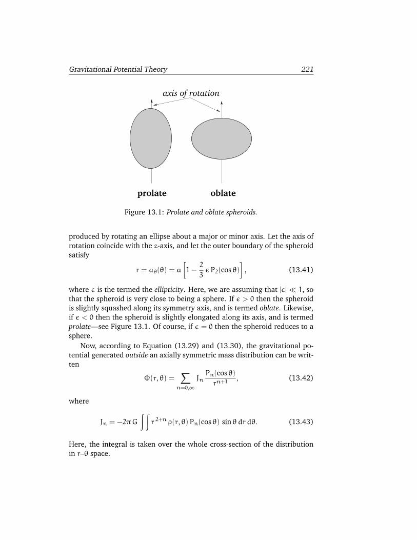
Gravitational Potential Theory 221
oblate
axis of rotation
prolate
Figure 13.1: Prolate and oblate spheroids.
produced by rotating an ellipse about a major or minor axis. Let the axis of
rotation coincide with the z-axis, and let the outer boundary of the spheroid
satisfy
r = aθ(θ) = a
[
1−2
3ǫ P2(cos θ)
]
, (13.41)
where ǫ is the termed the ellipticity. Here, we are assuming that |ǫ| ≪ 1, so
that the spheroid is very close to being a sphere. If ǫ > 0 then the spheroid
is slightly squashed along its symmetry axis, and is termed oblate. Likewise,
if ǫ < 0 then the spheroid is slightly elongated along its axis, and is termed
prolate—see Figure 13.1. Of course, if ǫ = 0 then the spheroid reduces to a
sphere.
Now, according to Equation (13.29) and (13.30), the gravitational po-
tential generated outside an axially symmetric mass distribution can be writ-
ten
Φ(r, θ) =∑
n=0,∞
JnPn(cos θ)
rn+1, (13.42)
where
Jn = −2πG
∫ ∫
r2+nρ(r, θ)Pn(cos θ) sin θdr dθ. (13.43)
Here, the integral is taken over the whole cross-section of the distribution
in r–θ space.

222 NEWTONIAN DYNAMICS
It follows that for a uniform spheroid
Jn = −2πGγ
∫π
0
Pn(cos θ)
∫aθ(θ)
0
r2+ndr sin θdθ (13.44)
Hence,
Jn = −2πGγ
(3+ n)
∫π
0
Pn(cos θ)a3+nθ (θ) sin θdθ, (13.45)
giving
Jn ≃ −2πGγa3+n
(3+ n)
∫π
0
Pn(cos θ)
[
P0(cos θ) −2
3(3+ n) ǫP2(cosθ)
]
sin θdθ,
(13.46)
to first-order in ǫ. It is thus clear, from Equation (13.26), that, to first-order
in ǫ, the only non-zero Jn are
J0 = −4πGγa3
3= −GM, (13.47)
J2 =8πGγa5ǫ
15=2
5GMa2ǫ, (13.48)
since M = (4π/3)a3γ.
Thus, the gravitational potential outside a uniform spheroid of total mass
M, mean radius a, and ellipticity ǫ, is
Φ(r, θ) = −GM
r+2
5
GMa2
r3ǫP2(cos θ) + O(ǫ2). (13.49)
In particular, the gravitational potential on the surface of the spheroid is
Φ(aθ, θ) = −GM
aθ+2
5
GMa2
a3θǫP2(cos θ) + O(ǫ2), (13.50)
which yields
Φ(aθ, θ) ≃ −GM
a
[
1+4
15ǫ P2(cos θ) + O(ǫ2)
]
, (13.51)
where use has been made of Equation (13.41).
So, let us now consider a self-gravitating spheroid of mass M, mean ra-
dius a, and ellipticity ǫ: e.g., a star, or a planet. Assuming, for the sake of
simplicity, that the spheroid is composed of uniform density incompressible
fluid, the gravitational potential on its surface is given by Equation (13.51).

Gravitational Potential Theory 223
However, the condition for an equilibrium state is that the potential be con-
stant over the surface. If this is not the case then there will be gravitational
forces acting tangential to the surface. Such forces cannot be balanced by in-
ternal pressure, which only acts normal to the surface. Hence, from (13.51),
it is clear that the condition for equilibrium is ǫ = 0. In other words, the
equilibrium configuration of a self-gravitating mass is a sphere. Deviations
from this configuration can only be caused by forces in addition to self-
gravity and internal pressure: e.g., centrifugal forces due to rotation, or
tidal forces due to orbiting masses.
13.6 Rotational Flattening
Let us consider the equilibrium configuration of a self-gravitating spheroid,
composed of uniform density incompressible fluid, which is rotating steadily
about some fixed axis. Let M be the total mass, a the mean radius, ǫ the
ellipticity, and Ω the angular velocity of rotation. Furthermore, let the axis
of rotation coincide with the axis of symmetry, which is assumed to run
along the z-axis.
Let us transform to a non-inertial frame of reference which co-rotates
with the spheroid about the z-axis, and in which the spheroid consequently
appears to be stationary. From Chapter 8, the problem is now analogous
to that of a non-rotating spheroid, except that the surface acceleration is
written g = gg+gc, where gg = −∇Φ(r, θ) is the gravitational acceleration,
and gc the centrifugal acceleration. The latter acceleration is of magnitude
r sin θΩ2, and is everywhere directed away from the axis of rotation (see
Figure 13.2 and Chapter 8). The acceleration thus has components
gc = rΩ2 sin θ (sin θ, cos θ, 0) (13.52)
in spherical polar coordinates. It follows that gc = −∇χ, where
χ(r, θ) = −Ω2 r2
2sin2θ = −
Ω2 r2
3[1− P2(cosθ)] (13.53)
can be thought of as a sort of centrifugal potential. Hence, the total surface
acceleration is
g = −∇(Φ+ χ). (13.54)
As before, the criterion for an equilibrium state is that the surface lie at
a constant total potential, so as to eliminate tangential surface forces which

224 NEWTONIAN DYNAMICS
cannot be balanced by internal pressure. Hence, assuming that the surface
satisfies Equation (13.41), the equilibrium configuration is specified by
Φ(aθ, θ) + χ(aθ, θ) = c, (13.55)
where c is a constant. It follows from Equations (13.51) and (13.53) that,
to first-order in ǫ and Ω2,
−GM
a
[
1+4
15ǫ P2(cos θ)
]
−Ω2a2
3[1− P2(cos θ)] ≃ c, (13.56)
which yields
ǫ =5
4
Ω2a3
GM. (13.57)
We conclude, from the above expression, that the equilibrium configu-
ration of a (relatively slowly) rotating self-gravitating mass distribution is
an oblate spheroid: i.e., a sphere which is slightly flattened along its axis of
rotation. The degree of flattening is proportional to the square of the ro-
tation rate. Now, from (13.41), the mean radius of the spheroid is a, the
radius at the poles (i.e., along the axis of rotation) is ap = a (1 − 2 ǫ/3),
and the radius at the equator (i.e., perpendicular to the axis of rotation) is
ae = a (1+ǫ/3)—see Figure 13.2. Hence, the degree of rotational flattening
can be writtenae− ap
a= ǫ =
5
4
Ω2a3
GM. (13.58)
Now, for the Earth, a = 6.37 × 10⁶m, Ω = 7.27 × 10⁻⁵ rad./s, and
M = 5.97× 1024kg. Thus, we predict that
ǫ = 0.00429, (13.59)
corresponding to a difference between equatorial and polar radii of
∆a = ae− ap = ǫa = 27.3 km. (13.60)
In fact, the observed degree of flattening of the Earth is ǫ = 0.00335, corre-
sponding to a difference between equatorial and polar radii of 21.4 km. The
main reason that our analysis has overestimated the degree of rotational
flattening of the Earth is that it models the terrestrial interior as a uniform
density incompressible fluid. In reality, the Earth’s core is much denser than
its crust. Moreover, the outer regions of the Earth are solid, and, therefore,
possesses some degree of elastic resistance to shape deformation.

Gravitational Potential Theory 225
axis of rotation
ae
gcap
Figure 13.2: Rotational flattening.
For Jupiter, a = 6.92 × 10⁷m, Ω = 1.76 × 10⁻⁴ rad./s, and M = 1.90 ×1027kg. Hence, we predict that
ǫ = 0.101. (13.61)
Note that this degree of flattening is much larger than that of the Earth, due
to Jupiter’s relatively large radius (about 10 times that of Earth), combined
with its relatively short rotation period (about 0.4 days). In fact, the polar
flattening of Jupiter is clearly apparent from images of this planet. The
observed degree of polar flattening of Jupiter is actually ǫ = 0.065. Our
estimate of ǫ is probably slightly too large because Jupiter, which is mostly
gaseous, does not rotate as a solid body.
13.7 McCullough’s Formula
According to Equations (13.43) and (13.48), if the Earth is modeled as
spheroid of uniform density γ then its ellipticity is given by
ǫ = −
∫
r2γP2(cos θ)d3r
/
I0,
= −1
2
∫
r2γ(
3 cos2θ− 1)
d3r
/
I0 (13.62)
where the integral is over the whole volume of the Earth, and I0 = (2/5)Ma2
would be the Earth’s moment of inertia were it exactly spherical. Now, the

226 NEWTONIAN DYNAMICS
Earth’s moment of inertia about its axis of rotation is given by
I‖ =
∫
(x2+ y2)γd3r =
∫
r2γ (1− cos2θ)d3r. (13.63)
Here, use has been made of Equations (13.9)–(13.11). Likewise, the Earth’s
moment of inertia about an axis perpendicular to its axis of rotation (and
passing through the Earth’s center) is
I⊥ =
∫
(y2+ z2)γd3r =
∫
r2γ (sin2θ sin2 φ+ cos2θ)d3r
=
∫
r2γ
(
1
2sin2θ+ cos2θ
)
d3r =1
2
∫
r2γ (1+ cos2θ)d3r,
(13.64)
since the average of sin2φ is 1/2 for an axisymmetric mass distribution. It
follows from the above three equations that
ǫ =I‖ − I⊥I0
≃I‖ − I⊥I‖
. (13.65)
This result, which is known as McCullough’s formula, demonstrates that the
Earth’s ellipticity is directly related to the difference between its principle
moment’s of inertia. It turns out that McCullough’s formula holds for any
axially symmetric mass distribution, and not just a spheroidal distribution
with uniform density. Finally, McCullough’s formula can be combined with
Equation (13.49) to give
Φ(r, θ) = −GM
r+G (I‖ − I⊥)
r3P2(cos θ). (13.66)
This is the general expression for the gravitational potential generated out-
side an axially symmetric mass distribution. The first term on the right-hand
side is the monopole gravitational field which would be generated if all of the
mass in the distribution were concentrated at its center of mass, whereas the
second term is the quadrupole field generated by any deviation from spheri-
cal symmetry in the distribution.
13.8 Tidal Elongation
Consider two point masses, m and m ′, executing circular orbits about their
common center of mass, C, with angular velocity ω. Let R be the distance

Gravitational Potential Theory 227
.
ρm′ m
R
C
Figure 13.3: Two orbiting masses.
between the masses, and ρ the distance between point C and mass m—see
Figure 13.3. We know, from Section 7.3, that
ω2 =GM
R3, (13.67)
and
ρ =m ′
MR, (13.68)
where M = m+m ′.Let us transform to a non-inertial frame of reference which rotates, about
an axis perpendicular to the orbital plane and passing through C, at the
angular velocity ω. In this reference frame, both masses appear to be sta-
tionary. Consider mass m. In the rotating frame, this mass experiences a
gravitational acceleration
ag =Gm ′
R2(13.69)
directed toward the center of mass, and a centrifugal acceleration (see Chap-
ter 8)
ac = ω2ρ (13.70)
directed away from the center of mass. However, it is easily demonstrated,
using Equations (13.67) and (13.68), that
ac = ag. (13.71)
In other words, the gravitational and centrifugal accelerations balance, as
must be the case if mass m is to remain stationary in the rotating frame.
Let us investigate how this balance is affected if the masses m and m ′ have
finite spatial extents.
Let the center of the mass distribution m ′ lie at A, the center of the
mass distribution m at B, and the center of mass at C—see Figure 13.4.
We wish to calculate the centrifugal and gravitational accelerations at some

228 NEWTONIAN DYNAMICS
R
θ
R′
A
D
BC
r
z
Figure 13.4: Calculation of tidal forces.
point D in the vicinity of point B. It is convenient to adopt spherical polar
coordinates, centered on point B, and aligned such that the z-axis coincides
with the line BA.
Let us assume that the mass distribution m is orbiting around C, but is
not rotating about an axis passing through its center, in order to exclude
rotational flattening from our analysis. If this is the case then it is easily
seen that each constituent point of m executes circular motion of angular
velocity ω and radius ρ—see Figure 13.5. Hence, each constituent point
experiences the same centrifugal acceleration: i.e.,
gc = −ω2ρ ez. (13.72)
It follows that
gc = −∇χ, (13.73)
where
χ = ω2ρ z (13.74)
is the centrifugal potential, and z = r cos θ. The centrifugal potential can
also be written
χ =Gm ′
R
r
RP1(cos θ). (13.75)
The gravitational acceleration at point D due to mass m ′ is given by
gg = −∇Φ ′, (13.76)
where the gravitational potential takes the form
Φ ′ = −Gm ′
R ′ . (13.77)
Here, R ′ is the distance between points A and D. Note that the gravita-
tional potential generated by the mass distribution m ′ is the same as that

Gravitational Potential Theory 229
B
ρ
ρB
BD
B
CC ′ DD
D
Figure 13.5: The center B of the mass distribution m orbits about the center
of mass C in a circle of radius ρ. If the mass distribution is non-rotating
then a non-central point D must maintain a constant spatial relationship to
B. It follows that point D orbits some point C ′, which has the same spatial
relationship to C that D has to B, in a circle of radius ρ.

230 NEWTONIAN DYNAMICS
generated by an equivalent point mass at A, as long as the distribution is
spherically symmetric, which we shall assume to be the case.
Now,
R ′ = R − r, (13.78)
where R ′ is the vector→DA, and R the vector
→BA—see Figure 13.4. It follows
that
R ′−1 =(
R2− 2R · r + r2)−1/2
=(
R2− 2 R r cosθ+ r2)−1/2
. (13.79)
Expanding in powers of r/R, we obtain
R ′−1 =1
R
∑
n=0,∞
(
r
R
)n
Pn(cos θ). (13.80)
Hence,
Φ ′ ≃ −Gm ′
R
[
1+r
RP1(cos θ) +
r2
R2P2(cos θ)
]
(13.81)
to second-order in r/R.
Adding χ and Φ ′, we obtain
χ+Φ ′ ≃ −Gm ′
R
[
1+r2
R2P2(cos θ)
]
(13.82)
to second-order in r/R. Note that χ + Φ ′ is the potential due to the net
external force acting on the mass distribution m. This potential is constant
up to first-order in r/R, because the first-order variations in χ and Φ ′ can-
cel one another. The cancellation is a manifestation of the balance between
the centrifugal and gravitational accelerations in the equivalent point mass
problem discussed above. However, this balance is only exact at the center
of the mass distribution m. Away from the center, the centrifugal accelera-
tion remains constant, whereas the gravitational acceleration increases with
increasing z. Hence, at positive z, the gravitational acceleration is larger
than the centrifugal, giving rise to a net acceleration in the +z-direction.
Likewise, at negative z, the centrifugal acceleration is larger than the gravi-
tational, giving rise to a net acceleration in the −z-direction. It follows that
the mass distribution m is subject to a residual acceleration, represented
by the second-order variation in Equation (13.82), which acts to elongate it
along the z-axis. This effect is known as tidal elongation.

Gravitational Potential Theory 231
a+m
′ R m
a−
Figure 13.6: Tidal elongation.
In order to calculate the tidal elongation of the mass distribution m we
need to add the potential, χ + Φ ′, due to the external forces, to the gravi-
tational potential, Φ, generated by the distribution itself. Assuming that the
mass distribution is spheroidal with mass m, mean radius a, and ellipticity
ǫ, it follows from Equations (13.41), (13.51), and (13.82) that the total
surface potential is given by
χ+Φ ′ +Φ ≃ −Gm
a−Gm ′
R
−4
15
Gm
aǫP2(cos θ) −
Gm ′ a2
R3P2(cos θ), (13.83)
where we have treated ǫ and a/R as small quantities. As before, the condi-
tion for equilibrium is that the total potential be constant over the surface
of the spheroid. Hence, we obtain
ǫ = −15
4
m ′
m
(
a
R
)3
(13.84)
as our prediction for the ellipticity induced in a self-gravitating spherical
mass distribution of total mass m and radius a by a second mass, m ′, which
is in a circular orbit of radius R about the distribution. Thus, if a+ is the
maximum radius of the distribution, and a− the minimum radius (see Fig-
ure 13.6), thena+ − a−
a= −ǫ =
15
4
m ′
m
(
a
R
)3
. (13.85)
Consider the tidal elongation of the Earth due to the Moon. In this case,
we have a = 6.37 × 10⁶m, R = 3.84 × 10⁸m, m = 5.97 × 1024kg, and
m ′ = 7.35× 10²²kg. Hence, we calculate that −ǫ = 2.1× 10⁻⁷, or
∆a = a+ − a− = −ǫa = 1.34m. (13.86)

232 NEWTONIAN DYNAMICS
We, thus, predict that tidal forces due to the Moon cause the Earth to elon-
gate along the axis joining its center to the Moon by about 1.3meters. Since
water is obviously more fluid than rock (especially on relatively short time-
scales) most of this elongation takes place in the oceans rather than in the
underlying land. Hence, the oceans rise, relative to the land, in the region
of the Earth closest to the Moon, and also in the region furthest away. Since
the Earth is rotating, whilst the tidal bulge of the oceans remains relatively
stationary, the Moon’s tidal force causes the ocean at a given point on the
Earth’s surface to rise and fall, by about a meter, twice daily, giving rise to
the phenomenon known as the tides.
Consider the tidal elongation of the Earth due to the Sun. In this case,
we have a = 6.37 × 10⁶m, R = 1.50 × 10¹¹m, m = 5.97 × 1024kg, and
m ′ = 1.99× 1030kg. Hence, we calculate that −ǫ = 9.6× 10⁻⁸, or
∆a = a+ − a− = −ǫa = 0.61m. (13.87)
Thus, the tidal elongation due to the Sun is about half that due to the Moon.
It follows that the tides are particularly high when the Sun, the Earth, and
the Moon lie approximately in a straight-line, so that the tidal effects of the
Sun and the Moon reinforce one another. This occurs at a new moon, or at
a full moon. These type of tides are called spring tides (note that the name
has nothing to do with the season). Conversely, the tides are particularly
low when the Sun, the Earth, and the Moon form a right-angle, so that the
tidal effects of the Sun and the Moon partially cancel one another. These
type of tides are called neap tides. Generally speaking, we would expect two
spring tides and two neap tides per month.
In reality, the amplitude of the tides varies significantly from place to
place on the Earth’s surface, due to the presence of the continents, which
impede the flow of the oceanic tidal bulge around the Earth. Moreover,
there is a time-lag of approximately 12 minutes between the Moon being
directly overhead (or directly below) and high tide, because of the finite
inertia of the oceans. Similarly, the time-lag between a spring tide and a full
moon, or a new moon, can be up to 2 days.
13.9 Roche Radius
Consider a spherical moon of mass m and radius a which is in a circular
orbit of radius R about a spherical planet of massm ′ and radius a ′. (Strictly
speaking, the moon and the planet execute circular orbits about their com-
mon center of mass. However, if the planet is much more massive than the

Gravitational Potential Theory 233
moon then the center of mass lies close to the planet’s center.) According to
the analysis in the previous section, a constituent element of the moon ex-
periences a force per unit mass, due to the gravitational field of the planet,
which takes the form
g ′ = −∇(χ+Φ ′), (13.88)
where
χ+Φ ′ = −Gm ′
R3(z2− x2/2− y2/2) + const. (13.89)
Here, (x, y, z) is a Cartesian coordinate system whose origin is the center of
the moon, and whose z-axis always points toward the center of the planet.
It follows that
g ′ =2Gm ′
R3
(
−x
2ex−
y
2ey+ z ez
)
. (13.90)
This so-called tidal force is generated by the spatial variation of the planet’s
gravitational field over the interior of the moon, and acts to elongate the
moon along an axis joining its center to that of the planet, and to compress
it in any direction perpendicular to this axis. Note that the magnitude of the
tidal force increases strongly as the radius, R, of the moon’s orbit decreases.
Now, if the tidal force is sufficiently strong then it can overcome the moon’s
self-gravity, and thereby rip the moon apart. It follows that there is a mini-
mum radius, generally referred to as the Roche radius, at which a moon can
orbit a planet without being destroyed by tidal forces.
Let us derive an expression for the Roche radius. Consider a small mass
element at the point on the surface of the moon which lies closest to the
planet, and at which the tidal force is consequently largest (i.e., x = y = 0,
z = a). According to Equation (13.90), the mass experiences an upward
(from the moon’s surface) tidal acceleration due to the gravitational attrac-
tion of the planet of the form
g ′ =2Gm ′ aR3
ez. (13.91)
The mass also experiences a downward gravitational acceleration due to the
gravitational influence of the moon which is written
g = −Gm
a2ez. (13.92)
Thus, the effective surface gravity at the point in question is
geff =Gm
a2
(
1− 2m ′
m
a3
R3
)
. (13.93)

234 NEWTONIAN DYNAMICS
Note that if R < Rc, where
Rc =
(
2m ′
m
)1/3
a, (13.94)
then the effective gravity is negative. In other words, the tidal force due to
the planet is strong enough to overcome surface gravity and lift objects off
the moon’s surface. If this is the case, and the tensile strength of the moon
is negligible, then it is fairly clear that the tidal force will start to break the
moon apart. Hence, Rc is the Roche radius. Now, m ′/m = (ρ ′/ρ) (a ′/a)3,
where ρ and ρ ′ are the mean mass densities of the moon and planet, respec-
tively. Thus, the above expression for the Roche radius can also be written
Rc = 1.41
(
ρ ′
ρ
)1/3
a ′. (13.95)
The above calculation is somewhat inaccurate, since it fails to take into
account the inevitable distortion of the moon’s shape in the presence of
strong tidal forces. (In fact, the calculation assumes that the moon always
remains spherical.) A more accurate calculation, which treats the moon as
a self-gravitating incompressible fluid, yields
Rc = 2.44
(
ρ ′
ρ
)1/3
a ′. (13.96)
It follows that if the planet and the moon have the same mean density then
the Roche radius is 2.44 times the planet’s radius. Note that small orbital
bodies such as rocks, or even very small moons, can survive intact within the
Roche radius because they are held together by internal tensile forces rather
than gravitational attraction. However, this mechanism becomes progres-
sively less effective as the size of the body in question increases. Not sur-
prisingly, virtually all large planetary moons occurring in the Solar System
have orbital radii which exceed the relevant Roche radius, whereas virtually
all planetary ring systems (which consist of myriads of small orbiting rocks)
have radii which lie inside the relevant Roche radius.
13.10 Precession of the Equinoxes
Consider the Earth-Sun system—see Figure 13.7. From a geocentric view-
point, the Sun orbits the Earth counter-clockwise (looking from the north),
once per year, in an approximately circular orbit of radius L = 1.50×10¹¹m.

Gravitational Potential Theory 235
L
Earth
ηSun
x
z
φ yΩ
θ
Figure 13.7: The Earth-Sun system.
In Astronomy, the plane of the Sun’s apparent orbit relative to the Earth is
known as the ecliptic plane. Let us define Cartesian coordinates centered
on the Earth such that the x- and y-axes lie in the ecliptic plane, and the
z-axis is normal to this plane (in the sense such that the Earth’s north pole
lies at positive z). It follows that the z-axis points toward a fixed point in
the sky (in the constellation Draco) known as the north ecliptic pole. It is
convenient to parameterize the instantaneous position of the Sun in terms
of a counter-clockwise azimuthal angle η—see Figure 13.7.
Let Ω be the Earth’s angular velocity vector due to its daily rotation. This
vector makes an angle θ with the z-axis, where θ = 23.44 is the inclination
of the ecliptic to the Earth’s equatorial plane. Suppose that the projection
of Ω onto the ecliptic plane makes an angle φ with the x-axis, where φ is
measured in a counter-clockwise sense—see Figure 13.7. The orientation
of the Earth’s axis of rotation (which is, of course, parallel to Ω) is thus
specified by the two angles θ and φ. Note, however, that these two angles
are also Euler angles, in the sense specified in Chapter 9. Let us examine the
Earth-Sun system at an instant in time when φ = 0: i.e., when Ω lies in the
x-z plane.
Now, according to Equation (13.66), the potential energy of the Earth-
Sun system is written
U = MsΦ = −GMsMe
L+GMs (I‖ − I⊥)
L3P2(γ), (13.97)
where Ms is the mass of the Sun, Me the mass of the Earth, I‖ the Earth’s
moment of inertia about its axis of rotation, and I⊥ the Earth’s moment of

236 NEWTONIAN DYNAMICS
inertia about an axis lying in its equatorial plane. Furthermore, γ is the
angle subtended between Ω and r, where r is the position vector of the Sun
relative to the Earth.
It is easily demonstrated that (with φ = 0)
Ω = Ω (sin θ, 0, cos θ), (13.98)
and
r = L (cosη, sinη, 0). (13.99)
Hence,
cosγ = cosη sin θ, (13.100)
giving
U = −GMsMe
L+GMs (I‖ − I⊥)
2 L3(3 cos2η sin2θ− 1). (13.101)
Now, on time-scales much longer than a year, we can average the above
expression over the Sun’s orbit to give
U = −GMsMe
L+GMs (I‖ − I⊥)
2 L3
(
3
2sin2θ− 1
)
(13.102)
(since the average of cos2η over a year is 1/2). Thus,
U = U0− α cos2θ, (13.103)
where U0 is a constant, and
α =3
4
GMs
L3(I‖ − I⊥). (13.104)
Here, Equation (13.103) represents the mean potential energy of the Earth
due to its gravitational interaction with the Sun.
Now, according to Section 9.9, the rotational kinetic energy of the Earth
can be written
K =1
2
(
I⊥ θ2+ I⊥ sin2θ φ2+ I‖Ω
2)
, (13.105)
where the Earth’s angular velocity
Ω = cosθ φ+ ψ (13.106)

Gravitational Potential Theory 237
is a constant of the motion. Here, ψ is the third Euler angle. Hence, the
Earth’s Lagrangian takes the form
L = K−U =1
2
(
I⊥ θ2+ I⊥ sin2θ φ2+ I‖Ω
2)
+ α cos2θ. (13.107)
One equation of motion which can immediately be derived from this La-
grangian isd
dt
(
∂L∂θ
)
−∂L∂θ
= 0, (13.108)
which reduces to
I⊥ θ−∂L∂θ
= 0. (13.109)
Consider steady precession, in which θ = 0, and φ and ψ are constants.
It follows, from the above equation, that such motion must satisfy the con-
straint∂L∂θ
= 0. (13.110)
Thus, we obtain
I⊥ sin θ cos θ φ2− I‖ sin θΩ φ− 2α sin θ cos θ = 0, (13.111)
where use has been made of Equations (13.106) and (13.107). It follows
that
I⊥ cos θ φ2− I‖Ωφ− 2α cos θ = 0. (13.112)
Now, |φ| ≪ Ω, so the above equation yields
φ ≃ −2α cos θ
I‖Ω= −
3
2
MsG
L3Ω
(
I‖ − I⊥I‖
)
cos θ
= −3
2
MsG
L3Ωǫ cos θ, (13.113)
where ǫ = 0.00335 is the Earth’s ellipticity, and use has been made of Equa-
tions (13.65) and (13.104). According to the above expression, the mutual
interaction between the Sun and the quadrupole gravitational field gener-
ated by the Earth’s slight oblateness causes the Earth’s axis of rotation to
precess steadily about the normal to the ecliptic plane at the rate φ. The fact
that φ is negative implies that the precession is in the opposite direction to
the directions of the Earth’s rotation and the Sun’s apparent orbit about the
Earth. Incidentally, the interaction causes a precession of the Earth’s rota-
tional axis, rather than the plane of the Sun’s orbit, because the Earth’s axial
moment of inertia is much less than the Sun’s orbital moment of inertia.

238 NEWTONIAN DYNAMICS
Now, the Sun’s apparent orbital angular velocity, ωs, about the Earth
satisfies
ω2s =GMs
L3. (13.114)
Hence,
φ
ωs= −
3
2
ωs
Ωǫ cosθ, (13.115)
and the precession period in years is given by
Ts(yr) =ωs
|φ|=2 To(day)
3 ǫ cos θ, (13.116)
where To(day) = Ω/ωs = 365.24 is the Sun’s orbital period in days. Thus,
given that ǫ = 0.00335 and θ = 23.44, we obtain
Ts = 79, 000 years. (13.117)
Using analogous arguments, we can also show that the Earth’s axis of
rotation precesses due to the interaction between the Moon and the Earth’s
quadrupole gravitational field. The precession rate is given by
φ = −3
2
MmG
R3Ωǫ cos θ, (13.118)
where Mm is the mass of the Moon, and R the mean distance between the
Moon and Earth. Now, the orbital angular velocity, ωm, of the Moon about
the Earth satisfies
ω2m =GMe
R3. (13.119)
Hence,
φ
ωs= −
3
2
ω2mωsΩ
Mm
Mecos θ, (13.120)
and the precession period in years is given by
Tm(yr) =ωs
|φ|= T 20
(
Me
Mm
)
Ts, (13.121)
where Me/Mm = 81.3 is the ratio of the mass of the Earth to that of the
Moon, and To = ωs/ωm = 0.081 is the Moon’s (synodic) orbit period in
years. It follows that
Tm = 0.53 Ts. (13.122)

Gravitational Potential Theory 239
Of course, the precession rates induced by the Sun and Moon are addi-
tive, giving rise to a net precession period, T , which satisfies
1
T=1
Ts+1
Tm. (13.123)
Thus, we finally obtain
T =Ts
2.88= 27, 000 years. (13.124)
According to the above analysis, the combined gravitational interaction
of the Sun and the Moon with the quadrupole field generated by the Earth’s
slight oblateness causes the Earth’s axis of rotation to precess steadily about
the normal to the ecliptic plane with a period of about 27,000 years. This
effect is known as the precession of the equinoxes. The observed period for
the precession of the equinoxes is actually 26,000 years. Our estimate is
slightly off because we neglected to take into account the small eccentricities
of the Earth’s orbit around the Sun, and the Moon’s orbit around the Earth.
We also neglected the fact that the Moon’s orbit is inclined by about 5 to
the ecliptic plane.
Now, the point in the sky toward which the Earth’s axis of rotation points
is known as the north celestial pole. Currently, this point lies within about
a degree of the fairly bright star Polaris, which is consequently sometimes
known as the north star or the pole star. It follows that Polaris appears to be
almost stationary in the sky, always lying due north, and can thus be used
for navigational purposes. Indeed, mariners have relied on the north star
for many hundreds of years to determine direction at sea. Unfortunately,
because of the precession of the equinoxes, the north celestial pole is not a
fixed point in the sky, but instead traces out a circle, of angular radius 23.44,about the north ecliptic pole, with a period of 26,000 years. Hence, a few
thousand years from now, the north celestial pole will no longer coincide
with Polaris, and there will be no convenient way of telling direction from
the stars.
The projection of the ecliptic plane onto the sky is called the ecliptic,
and coincides with the apparent path of the Sun against the backdrop of
the stars. Furthermore, the projection of the Earth’s equator onto the sky
is known as the celestial equator. The ecliptic is inclined at 23.44 to the
celestial equator. The two points in the sky at which the ecliptic crosses the
celestial equator are called the equinoxes, since night and day are equally
long when the Sun lies at these points. Thus, the Sun reaches the spring
equinox on about March 21st, and this traditionally marks the beginning of

240 NEWTONIAN DYNAMICS
Spring. Likewise, the Sun reaches the autumn equinox on about September
22nd, and this traditionally marks the beginning of Autumn. However, the
precession of the Earth’s axis of rotation causes the celestial equator (which
is always normal to this axis) to precess in the sky, and thus also produces
a precession of the equinoxes along the ecliptic—strictly speaking, it is this
effect which is known as the precession of the equinoxes. The direction of
the precession is opposite to the direction of the Sun’s apparent motion
around the ecliptic. Thus, in about 2000 BC, when the science of Astronomy
originated in ancient Egypt and Babylonia, the spring equinox lay in the
constellation Aries. Indeed, the spring equinox is still sometimes called the
first point of Aries in astronomical texts. About 90 BC, the spring equinox
moved into the constellation Pisces, where it still remains. The equinox will
move into the constellation Aquarius (marking the beginning of the much
heralded “Age of Aquarius”) in about 2600 AD. Incidentally, the position of
the spring equinox in the sky is of great importance in Astronomy, since it
is used as the zero of celestial longitude (much as Greenwich is used as the
zero of terrestrial longitude).
13.11 Potential Due to a Uniform Ring
Consider a uniform ring of mass M and radius r, centered on the origin,
and lying in the x-y plane. Let us consider the gravitational potential Φ(r)
generated by such a ring in the x-y plane (which corresponds to θ = 90).It follows, from Section 13.3, that for r > a,
Φ(r) = −GM
a
∑
n=0,∞
[Pn(0)]2
(
a
r
)n+1
. (13.125)
However, P0(0) = 1, P1(0) = 0, P2(0) = −1/2, P3(0) = 0, and P4(0) = 3/8.
Hence,
Φ(r) = −GM
r
[
1+1
4
(
a
r
)2
+9
64
(
a
r
)4
+ · · ·]
. (13.126)
Likewise, for r < a,
Φ(r) = −GM
a
∑
n=0,∞
[Pn(0)]2
(
r
a
)n
, (13.127)
giving
Φ(r) = −GM
a
[
1+1
4
(
r
a
)2
+9
64
(
r
a
)4
+ · · ·]
. (13.128)

Gravitational Potential Theory 241
13.12 Perihelion Precession of the Planets
The Solar System consists of eight major planets (Mercury to Neptune) mov-
ing around the Sun in slightly elliptical orbits which are approximately co-
planar with one another. According to Chapter 6, if we neglect the relatively
weak interplanetary gravitational interactions then the perihelia of the var-
ious planets (i.e., the points on their orbits at which they are closest to the
Sun) remain fixed in space. However, once these interactions are taken into
account, it turns out that the planetary perihelia all slowly precess around
the Sun. We can calculate the approximate rate of perihelion precession of
a given planet by treating the other planets as uniform concentric rings, cen-
tered on the Sun, of mass equal to the planetary mass, and radius equal to
the mean orbital radius.1 This is equivalent to averaging the interplanetary
gravitational interactions over the orbits of the other planets. It is reason-
able to do this, since the precession period in question is very much longer
than the orbital period of any planet in the Solar System. Thus, by treating
the other planets as rings, we can calculate the mean gravitational pertur-
bation due to these planets, and, thereby, determine the desired precession
rate.
We can conveniently index the planets in the Solar System such that
Mercury is planet 1, and Neptune planet 8. Let the Mi and the Ri, for
i = 1, 8, be the planetary masses and orbital radii, respectively. Furthermore,
letM0 be the mass of the Sun. It follows, from the previous section, that the
gravitational potential generated at the ith planet by the Sun and the other
planets is
Φ(Ri) = −GM0
Ri−G
∑
j<i
Mj
Ri
[
1+1
4
(
Rj
Ri
)2
+9
64
(
Rj
Ri
)4
+ · · ·]
−G∑
j>i
Mj
Rj
1+1
4
(
Ri
Rj
)2
+9
64
(
Ri
Rj
)4
+ · · ·
. (13.129)
Now, the radial force per unit mass acting on the ith planet is written f(Ri) =
−dΦ(Ri)/dr, giving
f(Ri) = −GM0
R2i−G
R2i
∑
j<i
Mj
[
1+3
4
(
Rj
Ri
)2
+45
64
(
Rj
Ri
)4
+ · · ·]
1M.G. Stewart, American Jou. Physics 73, 730 (2005).

242 NEWTONIAN DYNAMICS
+G
R2i
∑
j>i
Mj
(
Ri
Rj
)
1
2
(
Ri
Rj
)2
+9
16
(
Ri
Rj
)4
+ · · ·
. (13.130)
Hence, we obtain
Ri f′(Ri) =
2GM0
R2i+G
R2i
∑
j<i
Mj
[
2+ 3
(
Rj
Ri
)2
+135
32
(
Rj
Ri
)4
+ · · ·]
+G
R2i
∑
j>i
Mj
(
Ri
Rj
)
1
2
(
Ri
Rj
)2
+27
16
(
Ri
Rj
)4
+ · · ·
,
(13.131)
where ′ ≡ d/dr. It follows that
[
3+Ri f
′(Ri)f(Ri)
]−1/2
= (13.132)
1+3
4
∑
j<i
(
Mj
M0
)(
Rj
Ri
)2[
1+15
8
(
Rj
Ri
)2
+175
64
(
Rj
Ri
)4
+ · · ·]
+3
4
∑
j>i
(
Mj
M0
)
(
Ri
Rj
)3
1+15
8
(
Ri
Rj
)2
+175
64
(
Ri
Rj
)4
+ · · ·
.
Thus, according to Equation (6.104), the apsidal angle for the ith planet is
ψi = π
1+
3
4
∑
j<i
(
Mj
M0
)(
Rj
Ri
)2[
1+15
8
(
Rj
Ri
)2
+175
64
(
Rj
Ri
)4
+ · · ·]
+3
4
∑
j>i
(
Mj
M0
)
(
Ri
Rj
)3
1+15
8
(
Ri
Rj
)2
+175
64
(
Ri
Rj
)4
+ · · ·
.
(13.133)
Hence, the perihelion of the ith planet advances by
δψi =3π
2
∑
j<i
(
Mj
M0
)(
Rj
Ri
)2[
1+15
8
(
Rj
Ri
)2
+175
64
(
Rj
Ri
)4
+ · · ·]
+3π
2
∑
j>i
(
Mj
M0
)
(
Ri
Rj
)3
1+15
8
(
Ri
Rj
)2
+175
64
(
Ri
Rj
)4
+ · · ·
(13.134)

Gravitational Potential Theory 243
Planet M/M0 T(yr) R(au)
Mercury 1.66× 10⁻⁷ 0.241 0.387
Venus 2.45× 10⁻⁶ 0.615 0.723
Earth 3.04× 10⁻⁶ 1.000 1.00
Mars 3.23× 10⁻⁷ 1.881 1.52
Jupiter 9.55× 10⁻⁴ 11.86 5.20
Saturn 2.86× 10⁻⁴ 29.46 9.54
Uranus 4.36× 10⁻⁵ 84.01 19.19
Neptune 5.18× 10⁻⁵ 164.8 30.07
Table 13.1: Data for the major planets in the Solar System, giving the plane-
tary mass relative to that of the Sun, the orbital period in years, and the mean
orbital radius relative to that of the Earth.
radians per revolution around the Sun. Now, the time for one revolution is
Ti = 2π/ωi, where ω2i = GM0/R3i . Thus, the rate of perihelion precession,
in arc seconds per year, is given by
δψi =75
Ti(yr)
∑
j<i
(
Mj
M0
)(
Rj
Ri
)2[
1+15
8
(
Rj
Ri
)2
+175
64
(
Rj
Ri
)4
+ · · ·]
+∑
j>i
(
Mj
M0
)
(
Ri
Rj
)3
1+15
8
(
Ri
Rj
)2
+175
64
(
Ri
Rj
)4
+ · · ·
.
(13.135)
Table 13.2 and Figure 13.8 compare the observed perihelion precession
rates with the theoretical rates calculated from Equation (13.135) and the
planetary data given in Table 13.1. It can be seen that there is excellent
agreement between the two, except for the planet Venus. The main reason
for this is that Venus has an unusually low eccentricity (e = 0.0068), which
renders its perihelion point extremely sensitive to small perturbations.
13.13 Perihelion Precession of Mercury
If the calculation described in the previous section is carried out more accu-
rately, taking into account the slight eccentricities of the planetary orbits, as
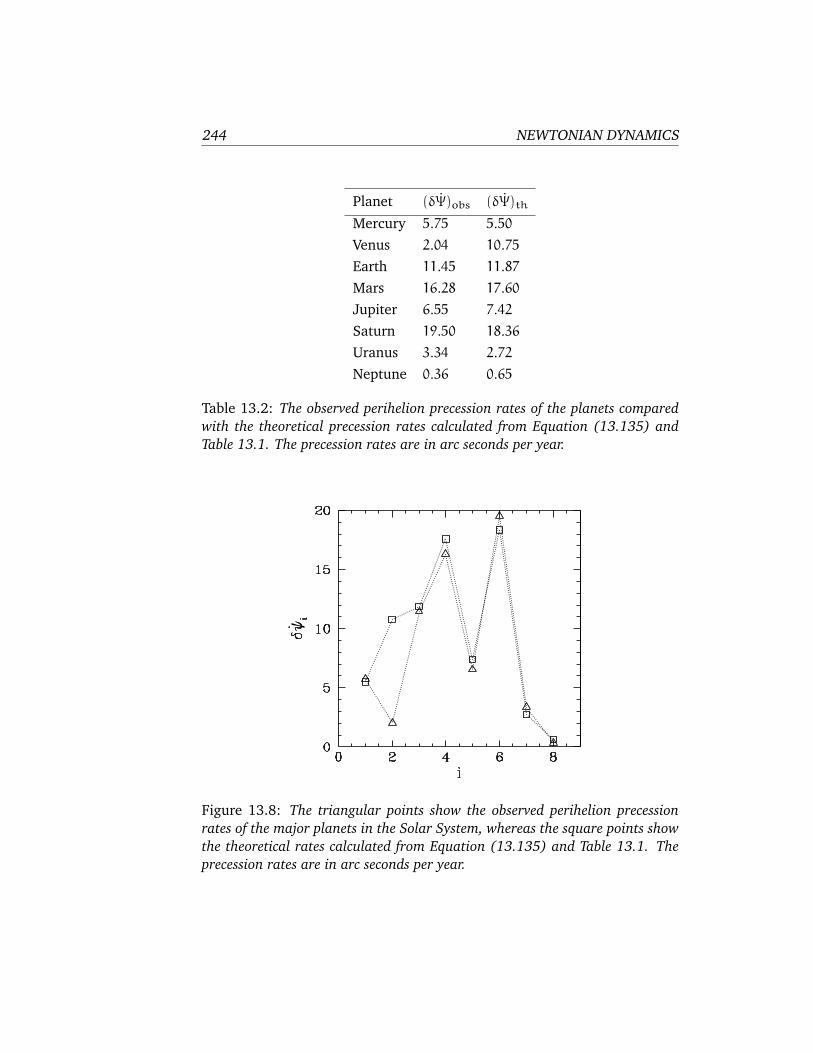
244 NEWTONIAN DYNAMICS
Planet (δΨ)obs (δΨ)th
Mercury 5.75 5.50
Venus 2.04 10.75
Earth 11.45 11.87
Mars 16.28 17.60
Jupiter 6.55 7.42
Saturn 19.50 18.36
Uranus 3.34 2.72
Neptune 0.36 0.65
Table 13.2: The observed perihelion precession rates of the planets compared
with the theoretical precession rates calculated from Equation (13.135) and
Table 13.1. The precession rates are in arc seconds per year.
Figure 13.8: The triangular points show the observed perihelion precession
rates of the major planets in the Solar System, whereas the square points show
the theoretical rates calculated from Equation (13.135) and Table 13.1. The
precession rates are in arc seconds per year.

Gravitational Potential Theory 245
well as their small mutual inclinations, and retaining many more terms in
the expansions (13.126) and (13.128), then the perihelion precession rate
of the planet Mercury is found to be 5.32 arc seconds per year. However, the
observed precession rate is 5.75 arc seconds per year. It turns out that the
cause of this discrepancy is the general relativistic correction to Newtonian
gravity.
General Relativity gives rise to a small correction to the force per unit
mass exerted by the Sun (mass M0) on a planet in a circular orbit of radius
r, and angular momentum per unit mass h. In fact, the modified formula
for f is
f ≃ −GM0
r2−3GM0h
2
c2 r4, (13.136)
where c is the velocity of light in vacuum. It follows that
r f ′
f= −2
(
1+3h2
c2 r2+ · · ·
)
. (13.137)
Hence, from Equation (6.104), the apsidal angle is
ψ ≃ π(
1+3h2
c2 r2
)
. (13.138)
Thus, the perihelion advances by
δψ ≃ 6πGM0
c2 r(13.139)
radians per revolution due to the general relativistic correction to Newto-
nian gravity. Here, use has been made of h2 = GM0 r. It follows that the
rate of perihelion precession due to the general relativistic correction is
δψ ≃ 0.0383
R T(13.140)
arc seconds per year, where R is the mean orbital radius in mean Earth or-
bital radii, and T is the orbital period in years. Hence, from Table 13.1, the
general relativistic contribution to δψ for Mercury is 0.41 arc seconds per
year. It is easily demonstrated that the corresponding contribution is negli-
gible for the other planets in the Solar System. If the above calculation is
carried out sightly more accurately, taking the eccentricity of Mercury’s orbit
into account, then the general relativistic contribution to δψ becomes 0.43
arc seconds per year. It follows that the total perihelion precession rate for

246 NEWTONIAN DYNAMICS
Mercury is 5.32+0.43 = 5.75 arc seconds per year. This is in exact agreement
with the observed precession rate. Indeed, the ability of General Relativity
to explain the discrepancy between the observed perihelion precession rate
of Mercury, and that calculated from Newtonian Dynamics, was one of the
first major successes of this theory.
13.14 Exercises
1. The Moon’s orbital period about the Earth is approximately 27.3 days, and isin the same direction as the Earth’s axial rotation (whose period is 24 hours).Use this data to show that high tides at a given point on the Earth occur every12 hours and 26 minutes.
2. Consider an artificial satellite in a circular orbit of radius L about the Earth.Suppose that the normal to the plane of the orbit subtends an angle θ withthe Earth’s axis of rotation. By approximating the orbiting satellite as a uni-form ring, demonstrate that the Earth’s oblateness causes the plane of thesatellite’s orbit to precess about the Earth’s rotational axis at the rate
φ
ω≃ −
1
2ǫ
(
R
L
)2
cos θ.
Here, ω is the satellite’s orbital angular velocity, ǫ = 0.00335 the Earth’sellipticity, and R the Earth’s radius. Note that the Earth’s axial moment ofinertial is I‖ ≃ (1/3)MR2, where M is the mass of the Earth.
3. A sun-synchronous satellite is one which always passes over a given point onthe Earth at the same local solar time. This is achieved by fixing the preces-sion rate of the satellite’s orbital plane such that it matches the rate at whichthe Sun appears to move against the background of the stars. What orbitalaltitude above the surface of the Earth would such a satellite need to havein order to fly over all latitudes between 50 N and 50 S? Is the direction ofthe satellite orbit in the same sense as the Earth’s rotation (prograde), or theopposite sense (retrograde)?

The Three-Body Problem 247
14 The Three-Body Problem
14.1 Introduction
We saw earlier, in Section 7.2, that an isolated dynamical system consisting
of two freely moving point masses exerting forces on one another—which
is usually referred to as a two-body problem—can always be converted into
an equivalent one-body problem. In particular, this implies that we can
exactly solve a dynamical system containing two gravitationally interacting
point masses, since the equivalent one-body problem is exactly soluble—see
Chapter 6 and Section 7.3. What about a system containing three gravita-
tionally interacting point masses? Despite hundreds of years of research,
no exact solution of this famous problem—which is generally known as the
three-body problem—has ever been found. It is, however, possible to make
some progress by severely restricting the problem’s scope.
14.2 Circular Restricted Three-Body Problem
Consider an isolated dynamical system consisting of three gravitationally
interacting point masses, m1, m2, and m3. Suppose, however, that the third
mass,m3, is so much smaller than the other two that it has a negligible effect
on their motion. Suppose, further, that the first two masses, m1 and m2,
execute circular orbits about their common center of mass. In the following,
we shall investigate this simplified problem, which is generally known as
the circular restricted three-body problem.
Let us define a Cartesian coordinate system (ξ, η, ζ) in an inertial ref-
erence frame whose origin coincides with the center of mass, C, of the two
orbiting masses. Furthermore, let the orbital plane of these masses coincide
with the ξ-η plane, and let them both lie on the ξ-axis at time t = 0—see
Figure 14.1. Suppose that R is the constant distance between the two orbit-
ing masses, r1 the constant distance between mass m1 and the origin, and
r2 the constant distance between mass m2 and the origin. Moreover, let ω
be the constant orbital angular velocity. It follows, from Section 7.3, that
ω2 =GM
R3, (14.1)
r1
r2=
m2
m1, (14.2)

248 NEWTONIAN DYNAMICS
R m2
m1
m3
C
ω tξ
η
r1
r2
Figure 14.1: The circular restricted three-body problem.
where M = m1+m2.
It is convenient to choose our unit of length such that R = 1, and our unit
of mass such that GM = 1. It follows, from Equation (14.1), that ω = 1.
However, we shall continue to retain ω in our equations, for the sake of
clarity. Let µ1 = Gm1, and µ2 = Gm2 = 1 − µ1. It is easily demonstrated
that r1 = µ2, and r2 = 1− r1 = µ1. Hence, the two orbiting masses, m1 and
m2, have position vectors r1 = (ξ1, η1, 0) and r2 = (ξ2, η2, 0), respectively,
where (see Figure 14.1)
r1 = µ2 (− cosωt, − sinωt, 0), (14.3)
r2 = µ1 (cosωt, sinωt, 0). (14.4)
Let the third mass have position vector r = (ξ, η, ζ). The Cartesian compo-
nents of the equation of motion of this mass are thus
ξ = −µ1(ξ− ξ1)
ρ31− µ2
(ξ− ξ2)
ρ32, (14.5)
η = −µ1(η− η1)
ρ31− µ2
(η− η2)
ρ32, (14.6)
ζ = −µ1ζ
ρ31− µ2
ζ
ρ32, (14.7)
where
ρ21 = (ξ− ξ1)2+ (η− η1)
2+ ζ2, (14.8)
ρ22 = (ξ− ξ2)2+ (η− η2)
2+ ζ2. (14.9)

The Three-Body Problem 249
14.3 Jacobi Integral
Consider the function
C = 2
(
µ1
ρ1+µ2
ρ2
)
+ 2ω (ξ η− η ξ) − ξ2− η2− ζ2. (14.10)
The time derivative of this function is written
C = −2µ1 ρ1
ρ21−2µ2 ρ2
ρ22+ 2ω (ξ η− η ξ) − 2 ξ ξ− 2 η η− 2 ζ ζ. (14.11)
Moreover, it follows, from Equations (14.3)–(14.4) and (14.8)–(14.9), that
ρ1 ρ1 = −(ξ1 ξ+ η1 η) +ω (ξη1− ηξ1) + ξ ξ+ η η+ ζ ζ,
(14.12)
ρ2 ρ2 = −(ξ2 ξ+ η2 η) +ω (ξη2− ηξ2) + ξ ξ+ η η+ ζ ζ.
(14.13)
Combining Equations (14.5)–(14.7) with the above three expressions, we
obtain (after considerable algebra)
C = 0. (14.14)
In other words, the function C—which is usually referred to as the Jacobi
integral—is a constant of the motion.
Now, we can rearrange Equation (14.10) to give
E ≡ 1
2(ξ2+ η2+ ζ2) −
(
µ1
ρ1+µ2
ρ2
)
= ω · h −C
2, (14.15)
where E is the energy (per unit mass) of mass m3, h = r× r its angular mo-
mentum (per unit mass), and ω = (0, 0, ω) the orbital angular velocity of
the other two masses. Note, however, that h is not a constant of the motion.
Hence, E is not a constant of the motion either. In fact, the Jacobi integral
is the only constant of the motion in the circular restricted three-body prob-
lem. Incidentally, the energy of massm3 is not a conserved quantity because
the other two masses in the system are moving.
14.4 Tisserand Criterion
Consider a dynamical system consisting of three gravitationally interacting
point masses, m1, m2, and m3. Let mass m1 represent the Sun, mass m2

250 NEWTONIAN DYNAMICS
the planet Jupiter, and mass m3 a comet. Since the mass of a comet is very
much less than that of the Sun or Jupiter, and the Sun and Jupiter are in
(almost) circular orbits about their common center of mass, the dynamical
system in question satisfies all of the necessary criteria to be considered an
example of a restricted three-body problem.
Now, the mass of the Sun is much greater than that of Jupiter. It follows
that the gravitational effect of Jupiter on the cometary orbit is negligible un-
less the comet makes a very close approach to Jupiter. Hence, as described
in Chapter 6, before and after such an approach the comet executes a stan-
dard elliptical orbit about the Sun with fixed orbital parameters: i.e., fixed
major radius, eccentricity, and inclination to the ecliptic plane. However, in
general, the orbital parameters before and after the close approach will not
be the same as one another. Let us investigate further.
Now, since m1≫ m2, we have µ1 = Gm1 ≃ G (m1+m2) = 1, and ρ1 ≃r. Hence, according to Equations (6.51) and (6.57), the (approximately)
conserved energy (per unit mass) of the comet before and after its close
approach to Jupiter is
E ≡ 1
2
(
ξ2+ η2+ ζ2)
−1
r= −
1
2 a. (14.16)
Note that the comet’s orbital energy is entirely determined by its major ra-
dius, a. (Incidentally, we are working in units such that the major radius of
Jupiter’s orbit is unity.) Furthermore, the (approximately) conserved angu-
lar momentum (per unit mass) of the comet before and after its approach to
Jupiter is written h, where h is directed normal to the comet’s orbital plane,
and, from Equations (6.27) and (6.47),
h2 = a (1− e2). (14.17)
Here, e is the comet’s orbital eccentricity. It follows that
ω · h = ωh cos I =√
a (1− e2) cos I, (14.18)
sinceω = 1 in our adopted system of units. Here, I is the angle of inclination
of the normal to the comet’s orbital plane to that of Jupiter’s orbital plane.
Let a, e, and I be the major radius, eccentricity, and inclination angle of
the cometary orbit before the close encounter with Jupiter, and let a ′, e ′,and I ′ be the corresponding parameters after the encounter. It follows from
Equations (14.15), (14.16), and (14.18), and the fact that C is conserved
during the encounter, whereas E and h are not, that
1
2 a+√
a (1− e2) cos I =1
2 a ′ +√
a ′ (1− e ′2) cos I ′. (14.19)

The Three-Body Problem 251
This result is known as the Tisserand criterion, and restricts the possible
changes in the orbital parameters of a comet due to a close encounter with
Jupiter (or any other massive planet).
The Tisserand criterion is very useful. For instance, whenever a new
comet is discovered, astronomers immediately calculate its Tisserand pa-
rameter,
TJ =1
a+ 2
√
a (1− e2) cos I. (14.20)
If this parameter has the same value as that of a previously observed comet
then it is quite likely that the new comet is, in fact, the same comet, but that
its orbital parameters have changed since it was last observed, due to a close
encounter with Jupiter. Incidentally, the subscript J in the above formula is
to remind us that we are dealing with the Tisserand parameter for close
encounters with Jupiter. (The parameter is, thus, evaluated in a system of
units in which the major radius of Jupiter’s orbit is unity). Obviously, it
is also possible to calculate Tisserand parameters for close encounters with
other planets.
The Tisserand criterion is also applicable to so-called gravity assists, in
which a space-craft gains energy due to a close encounter with a moving
planet. Such assists are often employed in missions to the outer planets to
reduce the amount of fuel which the space-craft must carry in order to reach
its destination. In fact, it is clear, from Equations (14.16) and (14.19), that
a space-craft can make use of a close encounter with a moving planet to
increase (or decrease) its orbital major radius a, and, hence, to increase (or
decrease) its total orbital energy.
14.5 Co-Rotating Frame
Let us transform to a non-inertial frame of reference rotating with angular
velocity ω about an axis normal to the orbital plane of masses m1 and m2,
and passing through their center of mass. It follows that masses m1 and
m2 appear stationary in this new reference frame. Let us define a Cartesian
coordinate system (x, y, z) in the rotating frame of reference which is such
that masses m1 and m2 always lie on the x-axis, and the z-axis is parallel
to the previously defined ζ-axis. It follows that masses m1 and m2 have
the fixed position vectors r1 = µ2 (−1, 0, 0) and r2 = µ1 (1, 0, 0) in our
new coordinate system. Finally, let the position vector of mass m3 be r =
(x, y, z)—see Figure 14.2.

252 NEWTONIAN DYNAMICS
.
µ1µ2
y
m1
m3
m2C
r
x
Figure 14.2: The co-rotating frame.
According to Chapter 8, the equation of motion of mass m3 in the rotat-
ing reference frame takes the form
r + 2ω × r = −µ1(r − r1)
ρ31− µ2
(r − r2)
ρ32− ω × (ω × r), (14.21)
where ω = (0, 0, ω), and
ρ21 = (x+ µ2)2+ y2+ z2, (14.22)
ρ22 = (x− µ1)2+ y2+ z2. (14.23)
Here, the second term on the left-hand side of Equation (14.21) is the Cori-
olis acceleration, whereas the final term on the right-hand side is the cen-
trifugal acceleration. The components of Equation (14.21) reduce to
x− 2ω y = −µ1 (x+ µ2)
ρ31−µ2 (x− µ1)
ρ32+ω2x, (14.24)
y+ 2ω x = −µ1y
ρ31−µ2y
ρ32+ω2y, (14.25)
z = −µ1 z
ρ31−µ2 z
ρ32, (14.26)
which yield
x− 2ω y = −∂U
∂x, (14.27)

The Three-Body Problem 253
y+ 2ω x = −∂U
∂y, (14.28)
z = −∂U
∂z, (14.29)
where
U = −µ1
ρ1−µ2
ρ2−ω2
2(x2+ y2) (14.30)
is the sum of the gravitational and centrifugal potentials.
Now, it follows from Equations (14.27)–(14.29) that
x x− 2ω x y = −x∂U
∂x, (14.31)
y y+ 2ω x y = −y∂U
∂y, (14.32)
z z = −z∂U
∂z. (14.33)
Summing the above three equations, we obtain
d
dt
[
1
2
(
x2+ y2+ z2)
+U
]
= 0. (14.34)
In other words,
C = −2U− v2 (14.35)
is a constant of the motion, where v2 = x2 + y2 + z2. In fact, C is the
Jacobi integral introduced in Section 14.3 [it is easily demonstrated that
Equations (14.10) and (14.35) are identical]. Note, finally, that the mass
m3 is restricted to regions in which
−2U ≥ C, (14.36)
since v2 is a positive definite quantity.
14.6 Lagrange Points
Let us search for possible equilibrium points of the mass m3 in the rotat-
ing reference frame. Such points are termed Lagrange points. Thus, in the
rotating frame, the mass m3 would remain at rest if placed at one of the
Lagrange points. It is, thus, clear that these points are fixed in the rotat-
ing frame. Conversely, in the inertial reference frame, the Lagrange points

254 NEWTONIAN DYNAMICS
rotate about the center of mass with angular velocity ω, and the mass m3would consequently also rotate about the center of mass with angular ve-
locity ω if placed at one of these points (with the appropriate velocity). In
the following, we shall assumed, without loss of generality, that m1 ≥ m2.The Lagrange points satisfy r = r = 0 in the rotating frame. It thus
follows, from Equations (14.27)–(14.29), that the Lagrange points are the
solutions of∂U
∂x=∂U
∂y=∂U
∂z= 0. (14.37)
Now, it is easily seen that
∂U
∂z=
(
µ1
ρ31+µ2
ρ32
)
z. (14.38)
Since the term in brackets is positive definite, we conclude that the only
solution to the above equation is z = 0. Hence, all of the Lagrange points lie
in the x-y plane.
If z = 0 then it is readily demonstrated that
µ1ρ21 + µ2ρ
22 = x2+ y2+ µ1µ2, (14.39)
where use has been made of the fact that µ1 + µ2 = 1. Hence, Equa-
tion (14.30) can also be written
U = −µ1
(
1
ρ1+ρ212
)
− µ2
(
1
ρ2+ρ222
)
+µ1µ2
2. (14.40)
The Lagrange points thus satisfy
∂U
∂x=
∂U
∂ρ1
∂ρ1
∂x+∂U
∂ρ2
∂ρ2
∂x= 0, (14.41)
∂U
∂y=
∂U
∂ρ1
∂ρ1
∂y+∂U
∂ρ2
∂ρ2
∂y= 0, (14.42)
which reduce to
µ1
(
1− ρ31ρ21
)
(
x+ µ2
ρ1
)
+ µ2
(
1− ρ32ρ22
)
(
x− µ1
ρ2
)
= 0, (14.43)
µ1
(
1− ρ31ρ21
)
(
y
ρ1
)
+ µ2
(
1− ρ32ρ22
)
(
y
ρ2
)
= 0. (14.44)

The Three-Body Problem 255
Now, one obvious solution of Equation (14.44) is y = 0, corresponding
to a Lagrange point which lies on the x-axis. It turns out that there are three
such points. L1 lies between masses m1 and m2, L2 lies to the right of mass
m2, and L3 lies to the left of mass m1—see Figure 14.2. At the L1 point, we
have x = −µ2+ρ1 = µ1−ρ2 and ρ1 = 1−ρ2. Hence, from Equation (14.43),
µ2
3µ1=
ρ32 (1− ρ2+ ρ22/3)
(1+ ρ2+ ρ22) (1− ρ2)3. (14.45)
Assuming that ρ2 ≪ 1, we can find an approximate solution of Equation
(14.45) by expanding in powers of ρ2:
α = ρ2+ρ223
+ρ323
+51 ρ4281
+ O(ρ52). (14.46)
This equation can be inverted to give
ρ2 = α−α2
3−α3
9−23α4
81+ O(α5), (14.47)
where
α =
(
µ2
3µ1
)1/3
. (14.48)
is assumed to be a small parameter.
At the L2 point, we have x = −µ2+ρ1 = µ1+ρ2 and ρ1 = 1+ρ2. Hence,
from Equation (14.43),
µ2
3µ1=ρ32 (1+ ρ2+ ρ22/3)
(1+ ρ2)2 (1− ρ32). (14.49)
Again, expanding in powers of ρ2, we obtain
α = ρ2−ρ223
+ρ323
+ρ4281
+ O(ρ52), (14.50)
ρ2 = α+α2
3−α3
9−31α4
81+ O(α5). (14.51)
Finally, at the L3 point, we have x = −µ2−ρ1 = µ1−ρ2 and ρ2 = 1+ρ1.
Hence, from Equation (14.43),
µ2
µ1=
(1− ρ31) (1+ ρ1)2
ρ31 (ρ21 + 3 ρ1+ 3). (14.52)

256 NEWTONIAN DYNAMICS
Let ρ1 = 1− β. Expanding in powers of β, we obtain
µ2
µ1=
12β
7+144β2
49+1567β3
343+ O(β4), (14.53)
β =7
12
(
µ2
µ1
)
−7
12
(
µ2
µ1
)2
+13223
20736
(
µ2
µ1
)3
+ O(
µ2
µ1
)4
,
(14.54)
where µ2/µ1 is assumed to be a small parameter.
Let us now search for Lagrange points which do not lie on the x-axis.
One obvious solution of Equations (14.41) and (14.42) is
∂U
∂ρ1=∂U
∂ρ2= 0, (14.55)
giving, from Equation (14.40),
ρ1 = ρ2 = 1, (14.56)
or
(x+ µ2)2+ y2 = (x− 1+ µ2)
2+ y2 = 1, (14.57)
since µ1 = 1− µ2. The two solutions of the above equation are
x =1
2− µ2, (14.58)
y = ±√3
2, (14.59)
and specify the positions of the Lagrange points designated L4 and L5. Note
that point L4 and the masses m1 and m2 lie at the apexes of an equilateral
triangle. The same is true for point L5. We have now found all of the possible
Lagrange points.
Figure 14.3 shows the positions of the two masses, m1 and m2, and the
five Lagrange points, L1 to L5, calculated for the case where µ2 = 0.1.
14.7 Zero-Velocity Surfaces
Consider the surface
V(x, y, z) = C, (14.60)
where
V = −2U =2µ1
ρ1+2µ2
ρ2+ x2+ y2. (14.61)

The Three-Body Problem 257
L3
L4
L5
L1
m2
L2
m1
Figure 14.3: The masses m1 and m2, and the five Lagrange points, L1 to L5,
calculated for µ2 = 0.1.
Note that V ≥ 0. It follows, from Equation (14.35), that if the mass m3 has
the Jacobi integral C, and lies on the surface specified in Equation (14.60),
then it must have zero velocity. Hence, such a surface is termed a zero-
velocity surface. The zero-velocity surfaces are important because they form
the boundary of regions from which the mass m3 is dynamically excluded:
i.e., regions in which V < C. Generally speaking, the regions from which
m3 is excluded grow in area as C increases, and vice versa.
Let Ci be the value of V at the Li Lagrange point, for i = 1, 5. When
µ2≪ 1, it is easily demonstrated that
C1 ≃ 3+ 34/3µ2/32 − 10µ2/3, (14.62)
C2 ≃ 3+ 34/3µ2/32 − 14µ2/3, (14.63)
C3 ≃ 3+ µ2, (14.64)
C4 ≃ 3− µ2, (14.65)
C4 ≃ 3− µ2. (14.66)
Note that C1 > C2 > C3 > C4 = C5.
Figures 14.4–14.8 show the intersection of the zero-velocity surface V =
C with the x-y plane for various different values of C, and illustrate how the
region from which m3 is dynamically excluded—which we shall term the

258 NEWTONIAN DYNAMICS
m2
m1
Figure 14.4: The zero-velocity surface V = C, where C > C1, calculated for
µ2 = 0.1. The massm3 is excluded from the region lying between the two inner
curves and the outer curve.
excluded region—evolves as the value of C is varied. Of course, any point
not in the excluded region is in the so-called allowed region. For C > C1, the
allowed region consists of two separate oval regions centered onm1 andm2,
respectively, plus an outer region which lies beyond a large circle centered
on the origin. All three allowed regions are separated from one another by
an excluded region—see Figure 14.4. When C = C1, the two inner allowed
regions merge at the L1 point—see Figure 14.5. When C = C2, the inner
and outer allowed regions merge at the L2 point, forming a horseshoe-like
excluded region—see Figure 14.6. When C = C3, the excluded region splits
in two at the L3 point—see Figure 14.7. For C4 < C < C3, the two excluded
regions are localized about the L4 and L5 points—see Figure 14.8. Finally,
for C < C4, there is no excluded region.
Figure 14.9 shows the zero-velocity surfaces and Lagrange points cal-
culated for the case µ2 = 0.01. It can be seen that, at very small values
of µ2, the L1 and L2 Lagrange points are almost equidistant from mass m2.
Furthermore, mass m2, and the L3, L4, and L5 Lagrange points all lie ap-
proximately on a unit circle, centered on mass m1. It follows that, when µ2is small, the Lagrange points L3, L4 and L5 all share the orbit of mass m2

The Three-Body Problem 259
m2
L1m1
Figure 14.5: The zero-velocity surface V = C, where C = C1, calculated for
µ2 = 0.1. The mass m3 is excluded from the region lying between the inner
and outer curves.
about m1 (in the inertial frame) with C3 being directly opposite m2, L4 (by
convention) 60 ahead of m2, and L5 60 behind.
14.8 Stability of Lagrange Points
We have seen that the five Lagrange points, L1 to L5, are the equilibrium
points of mass m3 in the co-rotating frame. Let us now determine whether
or not these equilibrium points are stable to small displacements.
Now, the equations of motion of mass m3 in the co-rotating frame are
specified in Equations (14.27)–(14.29). Note that the motion in the x-y
plane is complicated by presence of the Coriolis acceleration. However, the
motion parallel to the z-axis simply corresponds to motion in the potential
U. Hence, the condition for the stability of the Lagrange points (which all
lie at z = 0) to small displacements parallel to the z-axis is simply (see
Section 4.2)(
∂2U
∂z2
)
z=0
=µ1
ρ31+µ2
ρ32> 0. (14.67)
This condition is satisfied everywhere in the x-y plane. Hence, the Lagrange
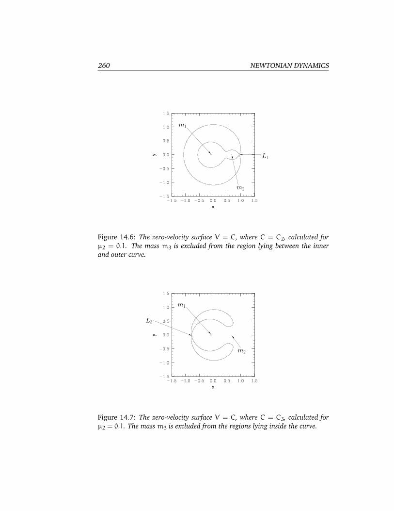
260 NEWTONIAN DYNAMICS
m1
m2
L1
Figure 14.6: The zero-velocity surface V = C, where C = C2, calculated for
µ2 = 0.1. The mass m3 is excluded from the region lying between the inner
and outer curve.
m2
m1
L3
Figure 14.7: The zero-velocity surface V = C, where C = C3, calculated for
µ2 = 0.1. The mass m3 is excluded from the regions lying inside the curve.

The Three-Body Problem 261
.
.
m2
L5
L4
m1
Figure 14.8: The zero-velocity surface V = C, where C4 < C < C3, calculated
for µ2 = 0.1. The mass m3 is excluded from the regions lying inside the two
curves.
points are all stable to small displacements parallel to the z-axis. It, thus,
remains to investigate their stability to small displacements lying within the
x-y plane.
Suppose that a Lagrange point is situated in the x-y plane at coordinates
(x0, y0, 0). Let us consider small amplitude x-ymotion in the vicinity of this
point by writing
x = x0+ δx, (14.68)
y = y0+ δy, (14.69)
z = 0, (14.70)
where δx and δy are infinitesimal. Expanding U(x, y, 0) about the Lagrange
point as a Taylor series, and retaining terms up to second-order in small
quantities, we obtain
U = U0+Uxδx+Uyδy+1
2Uxx (δx)2+Uxyδx δy+
1
2Uyy (δy)2, (14.71)
where U0 = U(x0, y0, 0), Ux = ∂U(x0, y0, 0)/∂x, Uxx = ∂2U(x0, y0, 0)/∂x2,
etc. However, by definition, Ux = Uy = 0 at a Lagrange point, so the

262 NEWTONIAN DYNAMICS
1L L2
L5
L3 M1
M
L4
2
Figure 14.9: The zero-velocity surfaces and Lagrange points calculated for
µ2 = 0.01.

The Three-Body Problem 263
expansion simplifies to
U = U0+1
2Uxx (δx)2+Uxyδx δy+
1
2Uyy (δy)2. (14.72)
Finally, substitution of Equations (14.68)–(14.70), and (14.72) into the
equations of x-y motion, (14.27) and (14.28), yields
δx− 2 δy = −Uxxδx−Uxyδy, (14.73)
δy+ 2 δx = −Uxyδx−Uyyδy, (14.74)
since ω = 1.
Let us search for a solution of the above pair of equations of the form
δx(t) = δx0 exp(γ t) and δy(t) = δy0 exp(γ t). We obtain
(
γ2+Uxx −2 γ+Uxy
2 γ+Uxy γ2+Uyy
)(
δx0
δy0
)
=
(
0
0
)
. (14.75)
This equation only has a non-trivial solution if the determinant of the matrix
is zero. Hence, we get
γ4+ (4+Uxx+Uyy)γ2+ (UxxUyy−U2xy) = 0. (14.76)
Now, it is convenient to define
A =µ1
ρ31+µ2
ρ32, (14.77)
B = 3
[
µ1
ρ51+µ2
ρ52
]
y2, (14.78)
C = 3
[
µ1 (x+ µ2)
ρ51+µ2 (x− µ1)
ρ52
]
y, (14.79)
D = 3
[
µ1 (x+ µ2)2
ρ31+µ2 (x− µ1)
2
ρ32
]
, (14.80)
where all terms are evaluated at the point (x0, y0, 0). It thus follows that
Uxx = A−D− 1, (14.81)
Uyy = A− B− 1, (14.82)
Uxy = −C. (14.83)

264 NEWTONIAN DYNAMICS
Consider the co-linear Lagrange points, L1, L2, and L3. These all lie
on the x-axis, and are thus characterized by y = 0, ρ21 = (x + µ2)2, and
ρ22 = (x − µ1)2. It follows, from the above equations, that B = C = 0 and
D = 3A. Hence, Uxx = −1 − 2A, Uyy = A − 1, and Uxy = 0. Equation
(14.76) thus yields
Γ2+ (2−A) Γ + (1−A) (1+ 2A) = 0, (14.84)
where Γ = γ2. Now, in order for a Lagrange point to be stable to small
displacements, all four of the roots, γ, of Equation (14.76) must be purely
imaginary. This, in turn, implies that the two roots of the above equation,
Γ =A− 2±
√
A (9A− 8)
2, (14.85)
must both be real and negative. Thus, the stability criterion is
8
9≤ A ≤ 1. (14.86)
Figure 14.10 shows A calculated at the three co-linear Lagrange points as
a function of µ2, for all allowed values of this parameter (i.e., 0 < µ2 ≤0.5). It can be seen that A is always greater than unity for all three points.
Hence, we conclude that the co-linear Lagrange points, L1, L2, and L3, are
intrinsically unstable equilibrium points in the co-rotating frame.
Let us now consider the triangular Lagrange points, L4 and L5. These
points are characterized by ρ1 = ρ2 = 1. It follows that A = 1, B = 9/4,
C = ±√
27/16 (1 − 2µ2), and D = 3/4. Hence, Uxx = −3/4, Uyy = −9/4,
and Uxy = ∓√
27/16 (1 − 2µ2), where the upper/lower signs corresponds
to L4 and L5, respectively. Equation (14.76) thus yields
Γ2+ Γ +27
4µ2 (1− µ2) = 0 (14.87)
for both points, where Γ = γ2. As before, the stability criterion is that the
two roots of the above equation must both be real and negative. This is the
case provided that 1 > 27µ2 (1− µ2), which yields the stability criterion
µ2 <1
2
1−
√
23
27
= 0.0385. (14.88)
In unnormalized units, this criterion becomes
m2
m1+m2< 0.0385. (14.89)

The Three-Body Problem 265
Figure 14.10: The solid, short-dashed, and long-dashed curves show A as a
function of µ2 at the L1, L2, and L3 Lagrange points.
We thus conclude that the L4 and L5 Lagrange points are stable equilib-
rium points, in the co-rotating frame, provided that mass m2 is less than
about 4% of mass m1. If this is the case then mass m3 can orbit around
these points indefinitely. In the inertial frame, the mass will share the or-
bit of mass m2 about mass m1, but will stay approximately 60 ahead of
mass m2, if it is orbiting the L4 point, or 60 behind, if it is orbiting the L5point—see Figure 14.9. This type of behavior has been observed in the Solar
System. For instance, there is a sub-class of asteroids, known as the Trojan
asteroids, which are trapped in the vicinity of the L4 and L5 points of the
Sun-Jupiter system (which easily satisfies the above stability criterion), and
consequently share Jupiter’s orbit around the Sun, staying approximately
60 ahead of, and 60 behind, Jupiter, respectively. Furthermore, the L4 and
L5 points of the Sun-Earth system are occupied by clouds of dust.

266 NEWTONIAN DYNAMICS

The Chaotic Pendulum 267
15 The Chaotic Pendulum
15.1 Introduction
Up until now, we have only dealt with dynamical problems which are ca-
pable of analytic solution. Let us now investigate a problem which is quite
intractable analytically, and in which meaningful progress can only be made
via numerical methods.
15.2 Basic Problem
Consider a simple pendulum consisting of a point mass m, at the end of
a light rigid rod of length l, attached to a fixed frictionless pivot which
allows the rod (and the mass) to move freely under gravity in the vertical
plane. Such a pendulum is sketched in Figure 15.1. Let us parameterize the
instantaneous position of the pendulum via the angle θ the rod makes with
the downward vertical. It is assumed that the pendulum is free to swing
through a full circle. Hence, θ and θ + 2π both correspond to the same
pendulum position.
The angular equation of motion of the pendulum is simply
mld2θ
dt2+mg sin θ = 0, (15.1)
where g is the downward acceleration due to gravity—see Section 4.10.
Suppose that the pendulum is embedded in a viscous medium (e.g., air). Let
us assume that the viscous drag torque acting on the pendulum is directly
proportional to the pendulum’s instantaneous velocity. It follows that, in the
presence of viscous drag, the above equation generalizes to
mld2θ
dt2+ ν
dθ
dt+mg sin θ = 0, (15.2)
where ν is a positive constant parameterizing the viscosity of the medium in
question—see Section 4.5. Of course, viscous damping will eventually drain
all energy from the pendulum, leaving it in a stationary state. In order to
maintain the motion against viscosity, it is necessary to add some external
driving. For the sake of simplicity, we choose a fixed amplitude periodic

268 NEWTONIAN DYNAMICS
l
m g
pivot point
fixed support
θ
m
T
Figure 15.1: A simple pendulum.
drive (which could arise, for instance, via periodic oscillations of the pen-
dulum’s pivot point). Thus, the final equation of motion of the pendulum is
written
mld2θ
dt2+ ν
dθ
dt+mg sin θ = A cos(ωt), (15.3)
where A and ω are constants parameterizing the amplitude and frequency
of the external driving torque, respectively.
Let
ω0 =
√
g
l. (15.4)
Of course, we recognize ω0 as the natural frequency of small amplitude os-
cillations of the pendulum. We can conveniently normalize the pendulum’s
equation of motion by writing,
t = ω0 t, (15.5)
ω =ω
ω0, (15.6)
Q =mg
ω0ν, (15.7)
A =A
mg, (15.8)
The Chaotic Pendulum 269
in which case Equation (15.3) becomes
d2θ
dt2+1
Q
dθ
dt+ sin θ = A cos(ω t). (15.9)
From now on, the hats on normalized quantities will be omitted, for ease
of notation. Note that, in normalized units, the natural frequency of small
amplitude oscillations is unity. Moreover, Q is the familiar quality-factor,
which is, roughly speaking, the number of oscillations of the undriven sys-
tem which must elapse before its energy is significantly reduced via the
action of viscosity—see Section 4.6. The quantity A is the amplitude of the
external torque measured in units of the maximum possible gravitational
torque. Finally, ω is the oscillation frequency of the external torque mea-
sured in units of the pendulum’s natural frequency.
Equation (15.9) is clearly a second-order ordinary differential equation.
It can, therefore, also be written as two coupled first-order ordinary differ-
ential equations:
dθ
dt= v, (15.10)
dv
dt= −
v
Q− sin θ+A cos(ωt). (15.11)
15.3 Analytic Solution
Before attempting a numerical solution of the equations of motion of any dy-
namical system, it is a good idea to, first, investigate the equations as thor-
oughly as possible via standard analytic techniques. Unfortunately, Equa-
tions (15.10) and (15.11) constitute a non-linear dynamical system—because
of the presence of the sin θ term on the right-hand side of Equation (15.11).
This system, like most non-linear systems, does not possess a simple analytic
solution. Fortunately, however, if we restrict our attention to small amplitude
oscillations, such that the approximation
sin θ ≃ θ (15.12)
is valid, then the system becomes linear, and can easily be solved analyti-
cally.
The linearized equations of motion of the pendulum take the form:
dθ
dt= v, (15.13)
dv
dt= −
v
Q− θ+A cos(ωt). (15.14)

270 NEWTONIAN DYNAMICS
Suppose that the pendulum’s position, θ(0), and velocity, v(0), are specified
at time t = 0. As is well-known, in this case, the above equations of motion
can be solved analytically to give:
θ(t) =
θ(0) −A (1−ω2)
[(1−ω2)2+ω2/Q2]
e−t/2Q cos(ω∗ t)
+1
ω∗
v(0) +θ(0)
2Q−
A (1− 3ω2)/2Q
[(1−ω2)2+ω2/Q2]
e−t/2Q sin(ω∗ t)
+A[
(1−ω2) cos(ωt) + (ω/Q) sin(ωt)]
[(1−ω2)2+ω2/Q2], (15.15)
v(t) =
v(0) −Aω2/Q
[(1−ω2)2+ω2/Q2]
e−t/2Q cosω∗t
−1
ω∗
θ(0) +v(0)
2Q−A [(1−ω2) −ω2/2Q2]
[(1−ω2)2+ω2/Q2]
e−t/2Q sin(ω∗ t)
+ωA
[
−(1−ω2) sin(ωt) + (ω/Q) cos(ωt)]
[(1−ω2)2+ω2/Q2]. (15.16)
Here,
ω∗ =
√
1−1
4Q2, (15.17)
and it is assumed that Q > 1/2. It can be seen that the above expressions
for θ and v both consist of three terms. The first two terms clearly represent
transients, since they depend on the initial conditions, and decay exponen-
tially in time—see Section 4.9. In fact, the e-folding time for the decay of
these terms is 2Q (in normalized time units). The final term represents the
time-asymptotic motion of the pendulum, and is manifestly independent of
the initial conditions—see Section 4.5.
It is often convenient to visualize the motion of a dynamical system as
an orbit, or trajectory, in phase-space, which is defined as the space of all
of the dynamical variables required to specify the instantaneous state of the
system. For the case in hand, there are two dynamical variables, v and θ, and
so phase-space corresponds to the θ-v plane. Note that each different point
in this plane corresponds to a unique instantaneous state of the pendulum.
[Strictly speaking, we should also consider t to be a dynamical variable,
since it appears explicitly on the right-hand side of Equation (15.11).]
It is clear, from Equations (15.15) and (15.16), that if we wait long
enough for all of the transients to decay away then the motion of the pen-

The Chaotic Pendulum 271
v /
A
/ Aθ
Figure 15.2: A phase-space plot of the periodic attractor for a linear damped
periodically driven pendulum. Data calculated analytically for Q = 4 and
ω = 2.
dulum settles down to the following simple orbit in phase-space:
θ(t) =A[
(1−ω2) cos(ωt) + (ω/Q) sin(ωt)]
[(1−ω2)2+ω2/Q2], (15.18)
v(t) =ωA
[
−(1−ω2) sin(ωt) + (ω/Q) cos(ωt)]
[(1−ω2)2+ω2/Q2]. (15.19)
This orbit traces out the closed curve(
θ
A
)2
+
(
v
ω A
)2
= 1, (15.20)
in phase-space, where
A =A
√
(1−ω2)2+ω2/Q2. (15.21)
As illustrated in Figure 15.2, this curve is an ellipse whose principal axes are
aligned with the v and θ coordinate axes. Observe that the curve is closed,
which suggests that the associated motion is periodic in time. In fact, the
motion repeats itself exactly every
τ =2π
ω(15.22)

272 NEWTONIAN DYNAMICS
ω
A /
A~
Figure 15.3: The maximum angular displacement of a linear damped peri-
odically driven pendulum as a function of driving frequency. The solid curve
corresponds to Q = 1. The short-dashed curve corresponds to Q = 5. The
long-dashed curve corresponds to Q = 10. Analytic data.
normalized time units. The maximum angular displacement of the pen-
dulum from its undriven rest position (θ = 0) is A. As illustrated in Fig-
ure 15.3, the variation of Awith driving frequencyω [see Equation (15.21)]
displays all of the features of a classic resonance curve. The maximum am-
plitude of the driven oscillation is proportional to the quality-factor, Q, and
is achieved when the driving frequency matches the natural frequency of
the pendulum (i.e., when |ω| = 1). Moreover, the width of the resonance in
ω-space is proportional to 1/Q—see Section 4.7.
The phase-space curve shown in Figure 15.2 is called a periodic attractor.
It is termed an “attractor” because, irrespective of the initial conditions, the
trajectory of the system in phase-space tends asymptotically to—in other
words, is attracted to—this curve as t → ∞. This gravitation of phase-space
trajectories towards the attractor is illustrated in Figures 15.4 and 15.5. Of
course, the attractor is termed “periodic” because it corresponds to motion
which is periodic in time.
Let us summarize our findings so far. We have discovered that if a
damped pendulum is subject to a low amplitude periodic drive then its time-
asymptotic response (i.e., its response after any transients have died away)
is periodic, with the same period as the driving torque. Moreover, the re-
sponse exhibits resonant behaviour as the driving frequency approaches the

The Chaotic Pendulum 273
v /
A
/ Aθ
Figure 15.4: The phase-space trajectory of a linear damped periodically driven
pendulum. Data calculated analytically for Q = 1 and ω = 2. Here, v(0)/A =
0 and θ(0)/A = 0.
v /
A
/ Aθ
Figure 15.5: The phase-space trajectory of a linear damped periodically driven
pendulum. Data calculated analytically for Q = 1 and ω = 2. Here, v(0)/A =
0.5 and θ(0)/A = 0.5.

274 NEWTONIAN DYNAMICS
natural frequency of oscillation of the pendulum. The amplitude of the res-
onant response, as well as the width of the resonant window, is governed by
the amount of damping in the system. After a little reflection, we can easily
appreciate that all of these results are a direct consequence of the linearity
of the pendulum’s equations of motion in the low amplitude limit. In fact, it
is easily demonstrated that the time-asymptotic response of any intrinsically
stable linear system (with a discrete spectrum of normal modes) to a peri-
odic drive is periodic, with the same period as the drive. Moreover, if the
driving frequency approaches one of the natural frequencies of oscillation
of the system then the response exhibits resonant behaviour. But, is this the
only allowable time-asymptotic response of a dynamical system to a peri-
odic drive? It turns out that it is not. Indeed, the response of a non-linear
system to a periodic drive is generally much richer and far more diverse
than simple periodic motion. Since the majority of naturally occurring dy-
namical systems are non-linear, it is clearly important that we gain a basic
understanding of this phenomenon. Unfortunately, we cannot achieve this
goal via a standard analytic approach, since non-linear equations of motion
generally do not possess simple analytic solutions. Instead, we must em-
ploy numerical methods. As an example, let us investigate the dynamics of
a damped pendulum, subject to a periodic drive, with no restrictions on the
amplitude of the pendulum’s motion.
15.4 Numerical Solution
In the following, we present numerical solutions of Equations (15.10) and
(15.11) obtained using a fairly standard fixed step-length fourth-order Runge-
Kutta integration scheme.1
15.5 Poincare Section
For the sake of definiteness, let us fix the normalized amplitude and fre-
quency of the external drive to be A = 1.5 and ω = 2/3, respectively.2
Furthermore, let us investigate any changes which may develop in the na-
ture of the pendulum’s time-asymptotic motion as the quality-factor Q is
varied. Of course, if Q is made sufficiently small (i.e., if the pendulum is
1W.H. Press, S.A. Teukolsky, W.T. Vetterling, and B.P. Flannery, Numerical recipes in C: The
art of scientific computing, 2nd Edition (Cambridge University Press, Cambridge UK, 1992),
Section 16.1.2G.L. Baker, Control of the chaotic driven pendulum, Am. J. Phys. 63, 832 (1995).

The Chaotic Pendulum 275
Figure 15.6: Equally spaced (in time) points on a time-asymptotic orbit in
phase-space. Data calculated numerically for Q = 0.5, A = 1.5, ω = 2/3,
θ(0) = 0, and v(0) = 0.
embedded in a sufficiently viscous medium) then we expect the amplitude
of the pendulum’s time-asymptotic motion to become low enough that the
linear analysis outlined in Section 15.3 is valid. Indeed, we expect non-
linear effects to manifest themselves as Q is gradually made larger, and the
amplitude of the pendulum’s motion consequently increases to such an ex-
tent that the small angle approximation breaks down.
Figure 15.6 shows a time-asymptotic orbit in phase-space calculated nu-
merically for a case where Q is sufficiently small (i.e., Q = 1/2) that the
small angle approximation holds reasonably well. Not surprisingly, the orbit
is very similar to the analytic orbits described in Section 15.3. The fact that
the orbit consists of a single loop, and forms a closed curve in phase-space,
strongly suggests that the corresponding motion is periodic with the same
period as the external drive—we term this type of motion period-1 motion.
More generally, period-n motion consists of motion which repeats itself ex-
actly every n periods of the external drive (and, obviously, does not repeat
itself on any time-scale less than n periods). Of course, period-1 motion is
the only allowed time-asymptotic motion in the small angle limit.
It would certainly be helpful to possess a graphical test for period-n mo-
tion. In fact, such a test was developed more than a hundred years ago by
the French mathematician Henry Poincare. Nowadays, it is called a Poincare
section in his honour. The idea of a Poincare section, as applied to a peri-

276 NEWTONIAN DYNAMICS
Figure 15.7: The Poincare section of a time-asymptotic orbit. Data calculated
numerically for Q = 0.5, A = 1.5, ω = 2/3, θ(0) = 0, v(0) = 0, and φ = 0.
odically driven pendulum, is very simple. As before, we calculate the time-
asymptotic motion of the pendulum, and visualize it as a series of points in
θ-v phase-space. However, we only plot one point per period of the external
drive. To be more exact, we only plot a point when
ωt = φ+ k 2π (15.23)
where k is any integer, and φ is referred to as the Poincare phase. For period-
1 motion, in which the motion repeats itself exactly every period of the
external drive, we expect the Poincare section to consist of only one point in
phase-space (i.e., we expect all of the points to plot on top of one another).
Likewise, for period-2 motion, in which the motion repeats itself exactly
every two periods of the external drive, we expect the Poincare section to
consist of two points in phase-space (i.e., we expect alternating points to plot
on top of one another). Finally, for period-n motion we expect the Poincare
section to consist of n points in phase-space.
Figure 15.7 displays the Poincare section of the orbit shown in Fig-
ure 15.6. The fact that the section consists of a single point confirms that
the motion displayed in Figure 15.6 is indeed period-1 motion.

The Chaotic Pendulum 277
Figure 15.8: The v-coordinate of the Poincare section of a time-asymptotic
orbit plotted against the quality-factor Q. Data calculated numerically for
A = 1.5, ω = 2/3, θ(0) = 0, v(0) = 0, and φ = 0.
15.6 Spatial Symmetry Breaking
Suppose that we now gradually increase the quality-factorQ. What happens
to the simple orbit shown in Figure 15.6? It turns out that, at first, noth-
ing particularly exciting happens. The size of the orbit gradually increases,
indicating a corresponding increase in the amplitude of the pendulum’s mo-
tion, but the general nature of the motion remains unchanged. However,
something interesting does occur when Q is increased beyond about 1.2.
Figure 15.8 shows the v-coordinate of the orbit’s Poincare section plotted
against Q in the range 1.2 and 1.3. Note the sharp downturn in the curve
at Q ≃ 1.245. What does this signify? Well, Figure 15.9 shows the time-
asymptotic phase-space orbit just before the downturn (i.e., at Q = 1.24),
and Figure 15.10 shows the orbit somewhat after the downturn (i.e., at
Q = 1.30). It is clear that the downturn is associated with a sudden change
in the nature of the pendulum’s time-asymptotic phase-space orbit. Prior to
the downturn, the orbit spends as much time in the region θ < 0 as in the
region θ > 0. However, after the downturn the orbit spends the majority
of its time in the region θ < 0. In other words, after the downturn, the
pendulum bob favours the region to the left of the pendulum’s vertical. This
is somewhat surprising, since there is nothing in the pendulum’s equations
of motion which differentiates between the regions to the left and to the
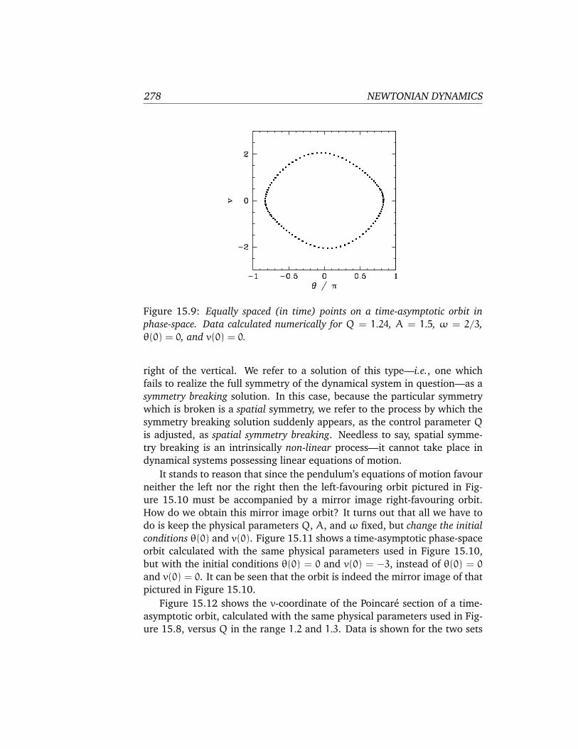
278 NEWTONIAN DYNAMICS
Figure 15.9: Equally spaced (in time) points on a time-asymptotic orbit in
phase-space. Data calculated numerically for Q = 1.24, A = 1.5, ω = 2/3,
θ(0) = 0, and v(0) = 0.
right of the vertical. We refer to a solution of this type—i.e., one which
fails to realize the full symmetry of the dynamical system in question—as a
symmetry breaking solution. In this case, because the particular symmetry
which is broken is a spatial symmetry, we refer to the process by which the
symmetry breaking solution suddenly appears, as the control parameter Q
is adjusted, as spatial symmetry breaking. Needless to say, spatial symme-
try breaking is an intrinsically non-linear process—it cannot take place in
dynamical systems possessing linear equations of motion.
It stands to reason that since the pendulum’s equations of motion favour
neither the left nor the right then the left-favouring orbit pictured in Fig-
ure 15.10 must be accompanied by a mirror image right-favouring orbit.
How do we obtain this mirror image orbit? It turns out that all we have to
do is keep the physical parameters Q, A, and ω fixed, but change the initial
conditions θ(0) and v(0). Figure 15.11 shows a time-asymptotic phase-space
orbit calculated with the same physical parameters used in Figure 15.10,
but with the initial conditions θ(0) = 0 and v(0) = −3, instead of θ(0) = 0
and v(0) = 0. It can be seen that the orbit is indeed the mirror image of that
pictured in Figure 15.10.
Figure 15.12 shows the v-coordinate of the Poincare section of a time-
asymptotic orbit, calculated with the same physical parameters used in Fig-
ure 15.8, versus Q in the range 1.2 and 1.3. Data is shown for the two sets

The Chaotic Pendulum 279
Figure 15.10: Equally spaced (in time) points on a time-asymptotic orbit in
phase-space. Data calculated numerically for Q = 1.30, A = 1.5, ω = 2/3,
θ(0) = 0, and v(0) = 0.
Figure 15.11: Equally spaced (in time) points on a time-asymptotic orbit in
phase-space. Data calculated numerically for Q = 1.30, A = 1.5, ω = 2/3,
θ(0) = 0, and v(0) = −3.

280 NEWTONIAN DYNAMICS
Figure 15.12: The v-coordinate of the Poincare section of a time-asymptotic
orbit plotted against the quality-factor Q. Data calculated numerically for
A = 1.5, and ω = 2/3. Data is shown for two sets of initial conditions:
θ(0) = 0 and v(0) = 0 (lower branch); and θ(0) = 0 and v(0) = −3 (upper
branch).
of initial conditions discussed above. The figure is interpreted as follows.
When Q is less than a critical value, which is about 1.245, then the two sets
of initial conditions lead to motions which converge on the same left-right
symmetric period-1 attractor. However, once Q exceeds the critical value
then the attractor bifurcates into two asymmetric mirror image period-1 at-
tractors. Obviously, the bifurcation is indicated by the forking of the curve
shown in Figure 15.12. The lower and upper branches correspond to the
left- and right-favouring attractors, respectively.
Spontaneous symmetry breaking, which is the fundamental non-linear
process illustrated in the above discussion, plays an important role in many
areas of Physics. For instance, symmetry breaking gives mass to elementary
particles in the unified theory of electromagnetic and weak interactions.3
Symmetry breaking also plays a pivotal role in the so-called “inflation” the-
ory of the expansion of the early universe.4
3E.S. Albers and B.W. Lee, Phys. Rep. 9C, 1 (1973).4P. Coles, and F. Lucchin, Cosmology: The origin and evolution of cosmic structure, (J. Wiley
& Sons, Chichester UK, 1995).

The Chaotic Pendulum 281
15.7 Basins of Attraction
We have seen that when Q = 1.3, A = 1.5, and ω = 2/3 there are two
co-existing period-1 attractors in θ–v phase-space. The time-asymptotic tra-
jectory of the pendulum through phase-space converges on one or other of
these attractors depending on the initial conditions: i.e., depending on the
values of θ(0) and v(0). Let us define the basin of attraction of a given at-
tractor as the locus of all points in the θ(0)–v(0) plane which lead to motion
which ultimately converges on that attractor. We have seen that in the low-
amplitude (i.e., linear) limit (see Section 15.3) there is only a single period-
1 attractor in phase-space, and all possible initial conditions lead to motion
which converges on this attractor. In other words, the basin of attraction
for the low-amplitude attractor constitutes the entire θ(0)–v(0) plane. The
present case, in which there are two co-existing attractors in phase-space, is
somewhat more complicated.
Figure 15.13 shows the basins of attraction, in θ(0)–v(0) space, of the
asymmetric mirror image attractors pictured in Figures 15.10 and 15.11.
The basin of attraction of the left-favoring attractor shown in Figure 15.10
is coloured black, whereas the basin of attraction of the right-favoring at-
tractor shown in Figure 15.11 is coloured white. It can be seen that the two
basins form a complicated interlocking pattern. Since we can identify the
angles π and −π, the right-hand edge of the pattern connects smoothly with
its left-hand edge. In fact, we can think of the pattern as existing on the
surface of a cylinder.
Suppose that we take a diagonal from the bottom left-hand corner of
Figure 15.13 to its top right-hand corner. This diagonal is intersected by a
number of black bands of varying thickness. Observe that the two narrowest
bands (i.e., the fourth band from the bottom left-hand corner and the second
band from the upper right-hand corner) both exhibit structure which is not
very well resolved in the present picture.
Figure 15.14 is a blow-up of a region close to the lower left-hand corner
of Figure 15.13. It can be seen that the unresolved band in the latter figure
(i.e., the second and third bands from the right-hand side in the former
figure) actually consists of a closely spaced pair of bands. Note, however,
that the narrower of these two bands exhibits structure which is not very
well resolved in the present picture.
Figure 15.15 is a blow-up of a region of Figure 15.14. It can be seen that
the unresolved band in the latter figure (i.e., the first and second bands from
the left-hand side in the former figure) actually consists of a closely spaced
pair of bands. Note, however, that the broader of these two bands exhibits

282 NEWTONIAN DYNAMICS
Figure 15.13: The basins of attraction for the asymmetric, mirror image,
attractors pictured in Figures 15.10 and 15.11. Regions of θ(0)–v(0) space
which lead to motion converging on the left-favouring attractor shown in Fig-
ure 15.10 are coloured white: regions of θ(0)–v(0) space which lead to motion
converging on the right-favouring attractor shown in Figure 15.11 are coloured
black. Data calculated numerically forQ = 1.3, A = 1.5,ω = 2/3, and φ = 0.
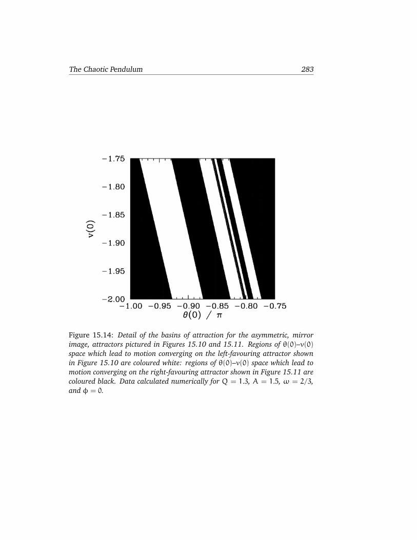
The Chaotic Pendulum 283
Figure 15.14: Detail of the basins of attraction for the asymmetric, mirror
image, attractors pictured in Figures 15.10 and 15.11. Regions of θ(0)–v(0)
space which lead to motion converging on the left-favouring attractor shown
in Figure 15.10 are coloured white: regions of θ(0)–v(0) space which lead to
motion converging on the right-favouring attractor shown in Figure 15.11 are
coloured black. Data calculated numerically for Q = 1.3, A = 1.5, ω = 2/3,
and φ = 0.

284 NEWTONIAN DYNAMICS
Figure 15.15: Detail of the basins of attraction for the asymmetric, mirror
image, attractors pictured in Figures 15.10 and 15.11. Regions of θ(0)–v(0)
space which lead to motion converging on the left-favouring attractor shown
in Figure 15.10 are coloured white: regions of θ(0)–v(0) space which lead to
motion converging on the right-favouring attractor shown in Figure 15.11 are
coloured black. Data calculated numerically for Q = 1.3, A = 1.5, ω = 2/3,
and φ = 0.

The Chaotic Pendulum 285
Figure 15.16: Detail of the basins of attraction for the asymmetric, mirror
image, attractors pictured in Figures 15.10 and 15.11. Regions of θ(0)–v(0)
space which lead to motion converging on the left-favouring attractor shown
in Figure 15.10 are coloured white: regions of θ(0)–v(0) space which lead to
motion converging on the right-favouring attractor shown in Figure 15.11 are
coloured black. Data calculated numerically for Q = 1.3, A = 1.5, ω = 2/3,
and φ = 0.

286 NEWTONIAN DYNAMICS
structure which is not very well resolved in the present picture.
Figure 15.16 is a blow-up of a region of Figure 15.15. It can be seen
that the unresolved band in the latter figure (i.e., the first, second, and
third bands from the right-hand side in the former figure) actually consists
of a closely spaced triplet of bands. Note, however, that the narrowest of
these bands exhibits structure which is not very well resolved in the present
picture.
It should be clear, by this stage, that no matter how closely we look at
Figure 15.13 we are going to find structure which we cannot resolve. In
other words, the separatrix between the two basins of attraction shown in
this figure is a curve which exhibits structure at all scales. Mathematicians
have a special term for such a curve—they call it a fractal.5
Many people think of fractals as mathematical toys whose principal use
is the generation of pretty pictures. However, it turns out that there is a
close connection between fractals and the dynamics of non-linear systems—
particularly systems which exhibit chaotic dynamics. We have just seen an
example in which the boundary between the basins of attraction of two co-
existing attractors in phase-space is a fractal curve. This turns out to be
a fairly general result: i.e., when multiple attractors exist in phase-space
the separatrix between their various basins of attraction is invariably frac-
tal. What is this telling us about the nature of non-linear dynamics? Well,
returning to Figure 15.13, we can see that in the region of phase-space in
which the fractal behaviour of the separatrix manifests itself most strongly
(i.e., the region where the light and dark bands fragment) the system ex-
hibits abnormal sensitivity to initial conditions. In other words, we only
have to change the initial conditions slightly (i.e., so as to move from a
dark to a light band, or vice versa) in order to significantly alter the time-
asymptotic motion of the pendulum (i.e., to cause the system to converge to
a left-favouring instead of a right-favouring attractor, or vice versa). Fractals
and extreme sensitivity to initial conditions are themes which will reoccur
in our investigation of non-linear dynamics.
15.8 Period-Doubling Bifurcations
Let us now return to Figure 15.8. Recall, that as the quality-factorQ is grad-
ually increased, the time-asymptotic orbit of the pendulum through phase-
space undergoes a sudden transition, at Q ≃ 1.245, from a left-right sym-
metric period-1 orbit to a left-favouring period-1 orbit. What happens if
5B.B. Mandelbrot, The fractal geometry of nature, (W.H. Freeman, New York NY, 1982).

The Chaotic Pendulum 287
Figure 15.17: The v-coordinate of the Poincare section of a time-asymptotic
orbit plotted against the quality-factor Q. Data calculated numerically for
A = 1.5, ω = 2/3, θ(0) = 0, v(0) = 0, and φ = 0.
we continue to increase Q? Figure 15.17 is basically a continuation of Fig-
ure 15.8. It can be seen that as Q is increased the left-favouring period-1
orbit gradually evolves until a critical value of Q, which is about 1.348, is
reached. When Q exceeds this critical value the nature of the orbit under-
goes another sudden change: this time from a left-favouring period-1 orbit
to a left-favouring period-2 orbit. Obviously, the change is indicated by the
forking of the curve in Figure 15.17. This type of transition is termed a
period-doubling bifurcation, since it involves a sudden doubling of the repe-
tition period of the pendulum’s time-asymptotic motion.
We can represent period-1 motion schematically as AAAAAA · · ·, where
A represents a pattern of motion which is repeated every period of the ex-
ternal drive. Likewise, we can represent period-2 motion as ABABAB · · ·,where A and B represent distinguishable patterns of motion which are re-
peated every alternate period of the external drive. A period-doubling bi-
furcation is represented: AAAAAA · · · → ABABAB · · ·. Clearly, all that
happens in such a bifurcation is that the pendulum suddenly decides to do
something slightly different in alternate periods of the external drive.
Figure 15.18 shows the time-asymptotic phase-space orbit of the pen-
dulum calculated for a value of Q somewhat higher than that required to
trigger the above mentioned period-doubling bifurcation. It can be seen that
the orbit is left-favouring (i.e., it spends the majority of its time on the left-

288 NEWTONIAN DYNAMICS
Figure 15.18: Equally spaced (in time) points on a time-asymptotic orbit in
phase-space. Data calculated numerically for Q = 1.36, A = 1.5, ω = 2/3,
θ(0) = 0, and v(0) = −3.
hand side of the plot), and takes the form of a closed curve consisting of two
interlocked loops in phase-space. Recall that for period-1 orbits there was
only a single closed loop in phase-space. Figure 15.19 shows the Poincare
section of the orbit shown in Figure 15.18. The fact that the section consists
of two points confirms that the orbit does indeed correspond to period-2
motion.
A period-doubling bifurcation is an example of temporal symmetry break-
ing. The equations of motion of the pendulum are invariant under the trans-
formation t → t + τ, where τ is the period of the external drive. In the low
amplitude (i.e., linear) limit, the time-asymptotic motion of the pendulum
always respects this symmetry. However, as we have just seen, in the non-
linear regime it is possible to obtain solutions which spontaneously break
this symmetry. Obviously, motion which repeats itself every two periods of
the external drive is not as temporally symmetric as motion which repeats
every period of the drive.
Figure 15.20 is essentially a continuation of Fig 15.12. Data is shown
for two sets of initial conditions which lead to motions converging on left-
favouring (lower branch) and right-favouring (upper branch) periodic at-
tractors. We have already seen that the left-favouring periodic attractor
undergoes a period-doubling bifurcation at Q = 1.348. It is clear from Fig-
ure 15.20 that the right-favouring attractor undergoes a similar bifurcation

The Chaotic Pendulum 289
Figure 15.19: The Poincare section of a time-asymptotic orbit. Data calculated
numerically for Q = 1.36, A = 1.5, ω = 2/3, θ(0) = 0, v(0) = 0, and φ = 0.
Figure 15.20: The v-coordinate of the Poincare section of a time-asymptotic
orbit plotted against the quality-factor Q. Data calculated numerically for
A = 1.5, ω = 2/3, and φ = 0. Data is shown for two sets of initial conditions:
θ(0) = 0 and v(0) = 0 (lower branch); and θ(0) = 0 and v(0) = −2 (upper
branch).

290 NEWTONIAN DYNAMICS
at almost exactly the same Q-value. This is hardly surprising since, as has
already been mentioned, for fixed physical parameters (i.e., Q, A, ω), the
left- and right-favouring attractors are mirror-images of one another.
15.9 Route to Chaos
Let us return to Figure 15.17, which tracks the evolution of a left-favouring
periodic attractor as the quality-factor Q is gradually increased. Recall that
when Q exceeds a critical value, which is about 1.348, then the attractor
undergoes a period-doubling bifurcation which converts it from a period-1
to a period-2 attractor. This bifurcation is indicated by the forking of the
curve in Figure 15.17. Let us now investigate what happens as we continue
to increaseQ. Figure 15.21 is basically a continuation of Figure 15.17. It can
be seen that, as Q is gradually increased, the attractor undergoes a period-
doubling bifurcation at Q = 1.348, as before, but then undergoes a second
period-doubling bifurcation (indicated by the second forking of the curves)
at Q ≃ 1.370, and a third bifurcation at Q ≃ 1.375. Obviously, the second
bifurcation converts a period-2 attractor into a period-4 attractor (hence,
two curves split apart to give four curves). Likewise, the third bifurcation
converts a period-4 attractor into a period-8 attractor (hence, four curves
split into eight curves). Shortly after the third bifurcation, the various curves
in the figure seem to expand explosively and merge together to produce an
area of almost solid black. As we shall see, this behaviour is indicative of
the onset of chaos.
Figure 15.22 is a blow-up of Figure 15.21, showing more details of the
onset of chaos. The period-4 to period-8 bifurcation can be seen quite
clearly. However, we can also see a period-8 to period-16 bifurcation, at
Q ≃ 1.3755. Finally, if we look carefully, we can see a hint of a period-16
to period-32 bifurcation, just before the start of the solid black region. Fig-
ures 15.21 and 15.22 seem to suggest that the onset of chaos is triggered by
an infinite series of period-doubling bifurcations.
Table 15.1 gives some details of the sequence of period-doubling bifur-
cations shown in Figures 15.21 and 15.22. Let us introduce a bifurcation
index n: the period-1 to period-2 bifurcation corresponds to n = 1; the
period-2 to period-4 bifurcation corresponds to n = 2; and so on. Let Qnbe the critical value of the quality-factor Q at which the nth bifurcation is
triggered. Table 15.1 shows the Qn, determined from Figures 15.21 and

The Chaotic Pendulum 291
Figure 15.21: The v-coordinate of the Poincare section of a time-asymptotic
orbit plotted against the quality-factor Q. Data calculated numerically for
A = 1.5, ω = 2/3, θ(0) = 0, v(0) = 0, and φ = 0.
15.22, for n = 1 to 5. Also shown is the ratio
Fn =Qn−1−Qn−2
Qn−Qn−1
(15.24)
for n = 3 to 5. It can be seen that Table 15.1 offers reasonably convincing
evidence that this ratio takes the constant value F = 4.69. It follows that we
can estimate the critical Q-value required to trigger the nth bifurcation via
the following formula:
Qn = Q1+ (Q2−Q1)
n−2∑
j=0
1
Fj, (15.25)
for n > 1. Note that the distance (in Q) between bifurcations decreases
rapidly as n increases. In fact, the above formula predicts an accumulation
of period-doubling bifurcations at Q = Q∞ , where
Q∞ = Q1+ (Q2−Q1)
∞∑
j=0
1
Fj≡ Q1+ (Q2−Q1)
F
F− 1= 1.3758. (15.26)

292 NEWTONIAN DYNAMICS
Figure 15.22: The v-coordinate of the Poincare section of a time-asymptotic
orbit plotted against the quality-factor Q. Data calculated numerically for
A = 1.5, ω = 2/3, θ(0) = 0, v(0) = 0, and φ = 0.
Note that our calculated accumulation point corresponds almost exactly to
the onset of the solid black region in Figure 15.22. By the time that Q
exceeds Q∞ , we expect the attractor to have been converted into a period-
infinity attractor via an infinite series of period-doubling bifurcations. A
period-infinity attractor is one whose corresponding motion never repeats
itself, no matter how long we wait. In dynamics, such bounded aperiodic
motion is generally referred to as chaos. Hence, a period-infinity attractor is
sometimes called a chaotic attractor. Now, period-n motion is represented
by n separate curves in Figure 15.22. It is, therefore, not surprising that
chaos (i.e., period-infinity motion) is represented by an infinite number of
curves which merge together to form a region of solid black.
Let us examine the onset of chaos in a little more detail. Figures 15.23–
15.26 show details of the pendulum’s time-asymptotic motion at various
stages on the period-doubling cascade discussed above. Figure 15.23 shows
period-4 motion: note that the Poincare section consists of four points, and
the associated sequence of net rotations per period of the pendulum re-
peats itself every four periods. Figure 15.24 shows period-8 motion: now
the Poincare section consists of eight points, and the rotation sequence re-

The Chaotic Pendulum 293
Bifurcation n Qn Qn−Qn−1 Fnperiod-1→period-2 1 1.34870 - -
period-2→period-4 2 1.37003 0.02133 -
period-4→period-8 3 1.37458 0.00455 4.69± 0.01period-8→period-16 4 1.37555 0.00097 4.69± 0.04period-16→period-32 5 1.37575 0.00020 4.9± 0.20
Table 15.1: The period-doubling cascade.
Figure 15.23: The Poincare section of a time-asymptotic orbit. Data calculated
numerically for Q = 1.372, A = 1.5, ω = 2/3, θ(0) = 0, v(0) = 0, and φ = 0.
Also, shown is the net rotation per period, ∆θ/2π, calculated at the Poincare
phase φ = 0.
peats itself every eight periods. Figure 15.25 shows period-16 motion: as
expected, the Poincare section consists of sixteen points, and the rotation
sequence repeats itself every sixteen periods. Finally, Figure 15.26 shows
chaotic motion. Note that the Poincare section now consists of a set of four
continuous line segments, which are, presumably, made up of an infinite
number of points (corresponding to the infinite period of chaotic motion).
Note, also, that the associated sequence of net rotations per period shows
no obvious sign of ever repeating itself. In fact, this sequence looks rather
like one of the previously shown periodic sequences with the addition of
a small random component. The generation of apparently random motion
from equations of motion, such as Equations (15.10) and (15.11), which
contain no overtly random elements is one of the most surprising features
of non-linear dynamics.
Many non-linear dynamical systems found in nature exhibit a transition

294 NEWTONIAN DYNAMICS
Figure 15.24: The Poincare section of a time-asymptotic orbit. Data calculated
numerically for Q = 1.375, A = 1.5, ω = 2/3, θ(0) = 0, v(0) = 0, and φ = 0.
Also, shown is the net rotation per period, ∆θ/2π, calculated at the Poincare
phase φ = 0.
Figure 15.25: The Poincare section of a time-asymptotic orbit. Data calculated
numerically for Q = 1.3757, A = 1.5, ω = 2/3, θ(0) = 0, v(0) = 0, and
φ = 0. Also, shown is the net rotation per period, ∆θ/2π, calculated at the
Poincare phase φ = 0.

The Chaotic Pendulum 295
Figure 15.26: The Poincare section of a time-asymptotic orbit. Data calculated
numerically for Q = 1.376, A = 1.5, ω = 2/3, θ(0) = 0, v(0) = 0, and φ = 0.
Also, shown is the net rotation per period, ∆θ/2π, calculated at the Poincare
phase φ = 0.
from periodic to chaotic motion as some control parameter is varied. More-
over, there are various known mechanisms by which chaotic motion can
arise from periodic motion. A transition to chaos via an infinite series of
period-doubling bifurcations, as illustrated above, is one of the most com-
monly occurring mechanisms. Around 1975, the physicist Mitchell Feigen-
baum was investigating a simple mathematical model, known as the logistic
map, which exhibits a transition to chaos, via a sequence of period-doubling
bifurcations, as a control parameter r is increased. Let rn be the value of r at
which the first 2n-period cycle appears. Feigenbaum noticed that the ratio
Fn =rn−1− rn−2
rn− rn−1
(15.27)
converges rapidly to a constant value, F = 4.669 . . ., as n increases. Feigen-
baum was able to demonstrate that this value of F is common to a wide
range of different mathematic models which exhibit transitions to chaos
via period-doubling bifurcations.6 Feigenbaum went on to argue that the
Feigenbaum ratio, Fn, should converge to the value 4.669 . . . in any dynami-
cal system exhibiting a transition to chaos via period-doubling bifurcations.7
This amazing prediction has been verified experimentally in a number of
6M.J. Feigenbaum, Quantitative universality for a class of nonlinear transformations, J.
Stat. Phys. 19, 25 (1978).7M.J. Feigenbaum, The universal metric properties of nonlinear transformations, J. Stat.
Phys. 21, 69 (1979).

296 NEWTONIAN DYNAMICS
quite different physical systems.8 Note that our best estimate of the Feigen-
baum ratio (see Table 15.1) is 4.69 ± 0.01, in good agreement with Feigen-
baum’s prediction.
The existence of a universal ratio characterizing the transition to chaos
via period-doubling bifurcations is one of many pieces of evidence indicating
that chaos is a universal phenomenon (i.e., the onset and nature of chaotic
motion in different dynamical systems has many common features). This
observation encourages us to believe that in studying the chaotic motion of
a damped periodically driven pendulum we are learning lessons which can
be applied to a wide range of non-linear dynamical systems.
15.10 Sensitivity to Initial Conditions
Suppose that we launch our pendulum and then wait until its motion has
converged onto a particular attractor. The subsequent motion can be visual-
ized as a trajectory θ0(t), v0(t) through phase-space. Suppose that we then
somehow perturb the pendulum, at time t = t0, such that its position in
phase-space is instantaneously changed from θ0(t0), v0(t0) to θ0(t0) + δθ0,
v0(t0) + δv0. The subsequent motion can be visualized as a second trajec-
tory θ1(t), v1(t) through phase-space. What is the relationship between the
original trajectory θ0(t), v0(t) and the perturbed trajectory θ1(t), v1(t)? In
particular, does the phase-space separation between the two trajectories,
whose components are
δθ(∆t) = θ1(t0+ ∆t) − θ0(t0+ ∆t), (15.28)
δv(∆t) = v1(t0+ ∆t) − v0(t0+ ∆t), (15.29)
grow in time, decay in time, or stay more or less the same? What we are
really investigating is how sensitive the time-asymptotic motion of the pen-
dulum is to initial conditions.
According to the linear analysis of Section 15.3,
δθ(∆t) = δθ0 cos(ω∗∆t) e−∆t/2Q
+1
ω∗
δv0+δθ0
2Q
sin(ω∗∆t) e−∆t/2Q, (15.30)
δv(∆t) = δv0 cos(ω∗∆t) e−∆t/2Q
−1
ω∗
δθ0+δv0
2Q
sin(ω∗∆t) e−∆t/2Q, (15.31)
8P. Citanovic, Universality in chaos, (Adam Hilger, Bristol UK, 1989).

The Chaotic Pendulum 297
Figure 15.27: The v-component of the separation between two neighbouring
phase-space trajectories (one of which lies on an attractor) plotted against nor-
malized time. Data calculated numerically for Q = 1.372, A = 1.5, ω = 2/3,
θ(0) = 0, and v(0) = 0. The separation between the two trajectories is initial-
ized to δθ0 = δv0 = 10−6 at ∆t = 0.
assuming sin(ω∗ t0) = 0. It is clear that, in the linear regime, at least,
the pendulum’s time-asymptotic motion is not particularly sensitive to ini-
tial conditions. In fact, if we move the pendulum’s phase-space trajectory
slightly off the linear attractor, as described above, then the perturbed trajec-
tory decays back to the attractor exponentially in time. In other words, if we
wait long enough then the perturbed and unperturbed motions of the pen-
dulum become effectively indistinguishable. Let us now investigate whether
this insensitivity to initial conditions carries over into the non-linear regime.
Figures 15.27–15.30 show the results of the experiment described above,
in which the pendulum’s phase-space trajectory is moved slightly off an at-
tractor and the phase-space separation between the perturbed and unper-
turbed trajectories is then monitored as a function of time, at various stages
on the period-doubling cascade discussed in the previous section. To be
more exact, the figures show the logarithm of the absolute magnitude of
the v-component of the phase-space separation between the perturbed and
unperturbed trajectories as a function of normalized time.
Figure 15.27 shows the time evolution of the v-component of the phase-
space separation, δv, between two neighbouring trajectories, one of which
is the period-4 attractor illustrated in Figure 15.23. It can be seen that

298 NEWTONIAN DYNAMICS
Figure 15.28: The v-component of the separation between two neighbouring
phase-space trajectories (one of which lies on an attractor) plotted against nor-
malized time. Data calculated numerically for Q = 1.375, A = 1.5, ω = 2/3,
θ(0) = 0, and v(0) = 0. The separation between the two trajectories is initial-
ized to δθ0 = δv0 = 10−6 at ∆t = 0.
Figure 15.29: The v-component of the separation between two neighbouring
phase-space trajectories (one of which lies on an attractor) plotted against nor-
malized time. Data calculated numerically for Q = 1.3757, A = 1.5, ω = 2/3,
θ(0) = 0, and v(0) = 0. The separation between the two trajectories is initial-
ized to δθ0 = δv0 = 10−6 at ∆t = 0.

The Chaotic Pendulum 299
Figure 15.30: The v-component of the separation between two neighbouring
phase-space trajectories (one of which lies on an attractor) plotted against nor-
malized time. Data calculated numerically for Q = 1.376, A = 1.5, ω = 2/3,
θ(0) = 0, and v(0) = 0. The separation between the two trajectories is initial-
ized to δθ0 = δv0 = 10−6 at ∆t = 0.
δv decays rapidly in time. In fact, the graph of log(|δv|) versus ∆t can be
plausibly represented as a straight-line of gradient λ. In other words,
|δv(∆t)| ≃ δv0 eλ∆t, (15.32)
where the quantity λ is known as the Liapunov exponent, and is obviously
negative. Clearly, in this case, λ measures the strength of the exponential
convergence of the two trajectories in phase-space. Of course, the graph
of log(|δv|) versus ∆t is not exactly a straight-line. There are deviations
due to the fact that δv oscillates, as well as decays, in time. There are also
deviations because the strength of the exponential convergence between the
two trajectories varies along the attractor.
The above definition of the Liapunov exponent is rather inexact, for two
main reasons. In the first place, the strength of the exponential conver-
gence/divergence between two neighbouring trajectories in phase-space,
one of which is an attractor, generally varies along the attractor. Hence,
we should really take formula (15.32) and somehow average it over the
attractor, in order to obtain a more unambiguous definition of λ. In the sec-
ond place, since the dynamical system under investigation is a second-order
system, it actually possesses two different Liapunov exponents. Consider the

300 NEWTONIAN DYNAMICS
evolution of an infinitesimal circle of perturbed initial conditions, centred on
a point in phase-space lying on an attractor. During its evolution, the circle
will become distorted into an infinitesimal ellipse. Let δk, where k = 1, 2, de-
note the phase-space length of the kth principal axis of the ellipse. The two
Liapunov exponents, λ1 and λ2, are defined via δk(∆t) ≃ δk(0) exp(λk∆t).
However, for large ∆t, the diameter of the ellipse is effectively controlled by
the Liapunov exponent with the most positive real part. Hence, when we
refer to the Liapunov exponent, λ, what we generally mean is the Liapunov
exponent with the most positive real part.
Figure 15.28 shows the time evolution of the v-component of the phase-
space separation, δv, between two neighbouring trajectories, one of which
is the period-8 attractor illustrated in Figure 15.24. It can be seen that δv
decays in time, though not as rapidly as in Figure 15.27. Another way of
saying this is that the Liapunov exponent of the periodic attractor shown in
Figure 15.24 is negative (i.e., it has a negative real part), but not as negative
as that of the periodic attractor shown in Figure 15.23.
Figure 15.29 shows the time evolution of the v-component of the phase-
space separation, δv, between two neighbouring trajectories, one of which
is the period-16 attractor illustrated in Figure 15.25. It can be seen that
δv decays weakly in time. In other words, the Liapunov exponent of the
periodic attractor shown in Figure 15.25 is small and negative.
Finally, Figure 15.30 shows the time evolution of the v-component of
the phase-space separation, δv, between two neighbouring trajectories, one
of which is the chaotic attractor illustrated in Figure 15.26. It can be seen
that δv increases in time. In other words, the Liapunov exponent of the
chaotic attractor shown in Figure 15.26 is positive. Further investigation
reveals that, as the control parameterQ is gradually increased, the Liapunov
exponent changes sign and becomes positive at exactly the same point that
chaos ensues in Figure 15.22.
The above discussion strongly suggests that periodic attractors are char-
acterized by negative Liapunov exponents, whereas chaotic attractors are
characterized by positive exponents. But, how can an attractor have a pos-
itive Liapunov exponent? Surely, a positive exponent necessarily implies
that neighbouring phase-space trajectories diverge from the attractor (and,
hence, that the attractor is not a true attractor)? It turns out that this is not
the case. The chaotic attractor shown in Figure 15.26 is a true attractor, in
the sense that neighbouring trajectories rapidly converge onto it—i.e., after
a few periods of the external drive their Poincare sections plot out the same
four-line segment shown in Figure 15.26. Thus, the exponential divergence
of neighbouring trajectories, characteristic of chaotic attractors, takes place
The Chaotic Pendulum 301
within the attractor itself. Obviously, this exponential divergence must come
to an end when the phase-space separation of the trajectories becomes com-
parable to the extent of the attractor.
A dynamical system characterized by a positive Liapunov exponent, λ,
has a time horizon beyond which regular deterministic prediction breaks
down. Suppose that we measure the initial conditions of an experimental
system very accurately. Obviously, no measurement is perfect: there is al-
ways some error δ0 between our estimate and the true initial state. After a
time t, the discrepancy grows to δ(t) ∼ δ0 exp(λ t). Let a be a measure of
our tolerance: i.e., a prediction within a of the true state is considered ac-
ceptable. It follows that our prediction becomes unacceptable when δ≫ a,
which occurs when
t > th ∼1
λln
(
a
δ0
)
. (15.33)
Note the logarithmic dependence on δ0. This ensures that, in practice, no
matter how hard we work to reduce our initial measurement error, we can-
not predict the behaviour of the system for longer than a few multiples of
1/λ.
It follows, from the above discussion, that chaotic attractors are associ-
ated with motion which is essentially unpredictable. In other words, if we at-
tempt to integrate the equations of motion of a chaotic system then even the
slightest error made in the initial conditions will be amplified exponentially
over time, and will rapidly destroy the accuracy of our prediction. Eventu-
ally, all that we will be able to say is that the motion lies somewhere on the
chaotic attractor in phase-space, but exactly where it lies on the attractor at
any given time will be unknown to us.
The hyper-sensitivity of chaotic systems to initial conditions is sometimes
called the butterfly effect. The idea is that a butterfly flapping its wings in a
South American rain-forest could, in principle, affect the weather in Texas
(since the atmosphere exhibits chaotic dynamics). This idea was first pub-
licized by the meteorologist Edward Lorenz, who constructed a very crude
model of the convection of the atmosphere when it is heated from below
by the ground.9 Lorenz discovered, much to his surprise, that his model
atmosphere exhibited chaotic motion—which, at that time, was virtually
unknown. In fact, Lorenz was essentially the first scientist to fully under-
stand the nature and ramifications of chaotic motion in physical systems.
In particular, Lorenz realized that the chaotic dynamics of the atmosphere
spells the doom of long-term weather forecasting: the best one can hope to
9E. Lorenz, Deterministic nonperiodic flow, J. Atmospheric Science 20, 130 (1963).

302 NEWTONIAN DYNAMICS
achieve is to predict the weather a few days in advance (1/λ for the atmo-
sphere is of order a few days).
15.11 Definition of Chaos
There is no universally agreed definition of chaos. However, most people
would accept the following working definition:
Chaos is aperiodic time-asymptotic behaviour in a deterministic
system which exhibits sensitive dependence on initial conditions.
This definition contains three main elements:
1. Aperiodic time-asymptotic behaviour—this implies the existence of
phase-space trajectories which do not settle down to fixed points or
periodic orbits. For practical reasons, we insist that these trajectories
are not too rare. We also require the trajectories to be bounded: i.e.,
they should not go off to infinity.
2. Deterministic—this implies that the equations of motion of the system
possess no random inputs. In other words, the irregular behaviour
of the system arises from non-linear dynamics, and not from noisy
driving forces.
3. Sensitive dependence on initial conditions—this implies that nearby
trajectories in phase-space separate exponentially fast in time: i.e.,
that the system has a positive Liapunov exponent.
15.12 Periodic Windows
Let us return to Figure 15.22. Recall, that this figure shows the onset of
chaos, via a cascade of period-doubling bifurcations, as the quality-factor
Q is gradually increased. Figure 15.31 is essentially a continuation of Fig-
ure 15.22 which shows the full extent of the chaotic region (inQ-v space). It
can be seen that the chaotic region ends abruptly when Q exceeds a critical
value, which is about 1.4215. Beyond this critical value, the time-asymptotic
motion appears to revert to period-1 motion (i.e., the solid black region col-
lapses to a single curve). It can also be seen that the chaotic region contains
many narrow windows in which chaos reverts to periodic motion (i.e., the
solid black region collapses to n curves, where n is the period of the mo-
tion) for a short interval in Q. The four widest windows are indicated in the
figure.

The Chaotic Pendulum 303
Figure 15.31: The v-coordinate of the Poincare section of a time-asymptotic
orbit plotted against the quality-factor Q. Data calculated numerically for
A = 1.5, ω = 2/3, θ(0) = 0, v(0) = −0.75, and φ = 0.
Figure 15.32 is a blow-up of the period-3 window shown in Figure 15.31.
It can be seen that the window appears “out of the blue” as Q is gradually
increased. However, it can also be seen that, as Q is further increased, the
window breaks down, and eventually disappears, due to the action of a cas-
cade of period-doubling bifurcations. The same basic mechanism operates
here as in the original period-doubling cascade, discussed in Section 15.9,
except that now the orbits are of period 3 · 2n, instead of 2 · 2n. Note that
all of the other periodic windows seen in Figure 15.31 break down in an
analogous manner, as Q is increased.
We now understand how periodic windows break down. But, how do
they appear in the first place? Figures 15.33–15.35 show details of the pen-
dulum’s time-asymptotic motion calculated just before the appearance of the
period-3 window (shown in Figure 15.32), just at the appearance of the
window, and just after the appearance of the window, respectively. It can be
seen, from Figure 15.33, that just before the appearance of the window the
attractor is chaotic (i.e., its Poincare section consists of a line, rather than
a discrete set of points), and the time-asymptotic motion of the pendulum
consists of intervals of period-3 motion interspersed with intervals of chaotic
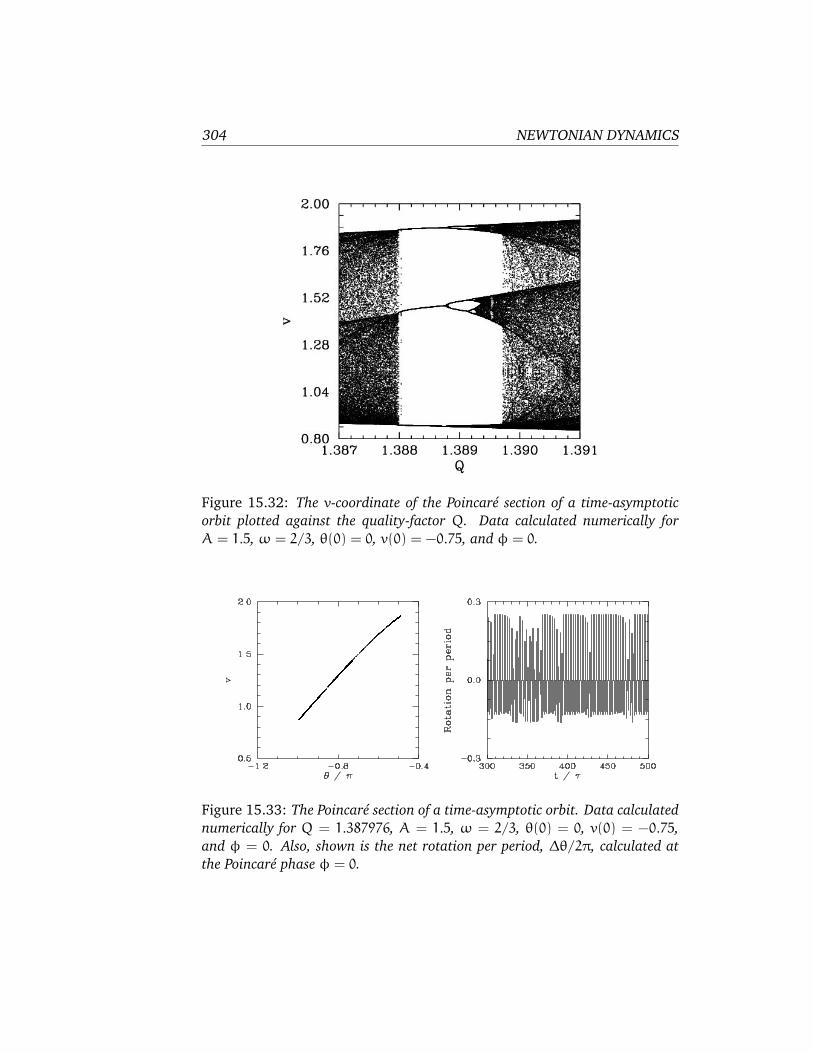
304 NEWTONIAN DYNAMICS
Figure 15.32: The v-coordinate of the Poincare section of a time-asymptotic
orbit plotted against the quality-factor Q. Data calculated numerically for
A = 1.5, ω = 2/3, θ(0) = 0, v(0) = −0.75, and φ = 0.
Figure 15.33: The Poincare section of a time-asymptotic orbit. Data calculated
numerically for Q = 1.387976, A = 1.5, ω = 2/3, θ(0) = 0, v(0) = −0.75,
and φ = 0. Also, shown is the net rotation per period, ∆θ/2π, calculated at
the Poincare phase φ = 0.

The Chaotic Pendulum 305
Figure 15.34: The Poincare section of a time-asymptotic orbit. Data calculated
numerically for Q = 1.387977, A = 1.5, ω = 2/3, θ(0) = 0, v(0) = −0.75,
and φ = 0. Also, shown is the net rotation per period, ∆θ/2π, calculated at
the Poincare phase φ = 0.
Figure 15.35: The Poincare section of a time-asymptotic orbit. Data calculated
numerically for Q = 1.387978, A = 1.5, ω = 2/3, θ(0) = 0, v(0) = −0.75,
and φ = 0. Also, shown is the net rotation per period, ∆θ/2π, calculated at
the Poincare phase φ = 0.

306 NEWTONIAN DYNAMICS
motion. Figure 15.34 shows that just at the appearance of the window the
attractor loses much of its chaotic nature (i.e., its Poincare section breaks
up into a series of points), and the chaotic intervals become shorter and
much less frequent. Finally, Figure 15.35 shows that just after the appear-
ance of the window the attractor collapses to a period-3 attractor, and the
chaotic intervals cease altogether. All of the other periodic windows seen in
Figure 15.31 appear in an analogous manner to that just described.
According to the above discussion, the typical time-asymptotic motion
seen just prior to the appearance of a period-n window consists of inter-
vals of period-n motion interspersed with intervals of chaotic motion. This
type of behaviour is called intermittency, and is observed in a wide variety
of non-linear systems. As we move away from the window, in parameter
space, the intervals of periodic motion become gradually shorter and more
infrequent. Eventually, they cease altogether. Likewise, as we move towards
the window, the intervals of periodic motion become gradually longer and
more frequent. Eventually, the whole motion becomes periodic.
In 1973, Metropolis and co-workers investigated a class of simple math-
ematical models which all exhibit a transition to chaos, via a cascade of
period-doubling bifurcations, as some control parameter r is increased.10
They were able to demonstrate that, for these models, the order in which
stable periodic orbits occur as r is increased is fixed. That is, stable periodic
attractors always occur in the same sequence as r is varied. This sequence is
called the universal or U-sequence. It is possible to make a fairly convincing
argument that any physical system which exhibits a transition to chaos via a
sequence of period-doubling bifurcations should also exhibit the U-sequence
of stable periodic attractors. Up to period-6, the U-sequence is
1, 2, 2× 2, 6, 5, 3, 2× 3, 5, 6, 4, 6, 5, 6.
The beginning of this sequence is familiar: periods 1, 2, 2 × 2 are the first
stages of the period-doubling cascade. (The later period-doublings give rise
to periods greater than 6, and so are omitted here). The next periods, 6, 5, 3
correspond to the first three periodic windows shown in Figure 15.31. Pe-
riod 2×3 is the first component of the period-doubling cascade which breaks
up the period-3 window. The next period, 5, corresponds to the last peri-
odic window shown in Figure 15.31. The remaining periods, 6, 4, 6, 5, 6,
correspond to tiny periodic windows, which, in practice, are virtually im-
possible to observe. It follows that our driven pendulum system exhibits
10N. Metropolis, M.L. Stein, and P.R. Stein, On finite limit sets for transformations on the
unit interval, J. Combin. Theor. 15, 25 (1973).

The Chaotic Pendulum 307
Figure 15.36: The v-coordinate of the Poincare section of a time-asymptotic
orbit plotted against the quality-factor Q. Data calculated numerically for
A = 1.5, ω = 2/3, θ(0) = 0, v(0) = 0, and φ = 0.
the U-sequence of stable periodic orbits fairly convincingly. This sequence
has also been observed experimentally in other, quite different, dynamical
systems.11 The existence of a universal sequence of stable periodic orbits
in dynamical systems which exhibit a transition to chaos via a cascade of
period-doubling bifurcations is another indication that chaos is a universal
phenomenon.
15.13 Further Investigation
Figure 15.36 shows the complete bifurcation diagram for the damped, peri-
odically driven, pendulum (with A = 1.5 and ω = 2/3). It can be seen that
the chaotic region investigated in the previous section is, in fact, the first,
and least extensive, of three different chaotic regions.
The interval between the first and second chaotic regions is occupied
by the period-1 orbits shown in Figure 15.37. Note that these orbits differ
somewhat from previously encountered period-1 orbits in that the pendu-
11R.H. Simoyi, A. Wolf, and H.L. Swinney, One-dimensional dynamics in a multi-component
chemical reaction, Phys. Rev. Lett. 49, 245 (1982).

308 NEWTONIAN DYNAMICS
Figure 15.37: Equally spaced (in time) points on a time-asymptotic orbit in
phase-space. Data calculated numerically for Q = 1.5, A = 1.5, ω = 2/3,
θ(0) = 0, and v(0) = 0. Also shown is the time-asymptotic orbit calculated for
the modified initial conditions θ(0) = 0, and v(0) = −1.
lum executes a complete rotation (either to the left or to the right) every
period of the external drive. Now, an n, l periodic orbit is defined such that
θ(t+ nτ) = θ(t) + 2π l
for all t (after the transients have died away). It follows that all of the pe-
riodic orbits which we encountered in previous sections were l = 0 orbits:
i.e., their associated motions did not involve a net rotation of the pendulum.
The orbits show in Figure 15.37 are n = 1, l = −1 and n = 1, l = +1 orbits,
respectively. The existence of periodic orbits in which the pendulum under-
goes a net rotation, either to the left or to the right, is another example of
spatial symmetry breaking—there is nothing in the pendulum’s equations of
motion which distinguishes between the two possible directions of rotation.
Figure 15.38 shows the Poincare section of a typical attractor in the sec-
ond chaotic region shown in Figure 15.36. It can be seen that this attractor
is far more convoluted and extensive than the simple 4-line chaotic attrac-
tor pictured in Figure 15.26. In fact, the attractor shown in Figure 15.38 is
clearly a fractal curve. It turns out that virtually all chaotic attractors exhibit
fractal structure.
The interval between the second and third chaotic regions shown in Fig-
ure 15.36 is occupied by n = 3, l = 0 periodic orbits. Figure 15.39 shows
the Poincare section of a typical attractor in the third chaotic region. It can
be seen that this attractor is even more overtly fractal in nature than that

The Chaotic Pendulum 309
Figure 15.38: The Poincare section of a time-asymptotic orbit. Data calculated
numerically for Q = 2.13, A = 1.5, ω = 2/3, θ(0) = 0, v(0) = 0, and φ = 0.
pictured in the previous figure. Note that the fractal nature of chaotic attrac-
tors is closely associated with some of their unusual properties. Trajectories
on a chaotic attractor remain confined to a bounded region of phase-space,
and yet they separate from their neighbours exponentially fast (at least, ini-
tially). How can trajectories diverge endlessly and still stay bounded? The
basic mechanism is described below. If we imagine a blob of initial condi-
tions in phase-space then these undergo a series of repeated stretching and
folding episodes, as the chaotic motion unfolds. The stretching is what gives
rise to the divergence of neighbouring trajectories. The folding is what en-
sures that the trajectories remain bounded. The net result is a phase-space
structure which looks a bit like filo pastry—in other words, a fractal struc-
ture.

310 NEWTONIAN DYNAMICS
Figure 15.39: The Poincare section of a time-asymptotic orbit. Data calculated
numerically for Q = 3.9, A = 1.5, ω = 2/3, θ(0) = 0, v(0) = 0, and φ = 0.