Non Newtonian Fluid Dynamics - PDHonline.com · Non Newtonian Fluid Dynamics ... laminar and turbulent flow and pressure drop calculation methods. The calculation methods to measure

PDHonline Course M417 (3 PDH)

Non Newtonian Fluid Dynamics

2012

Instructor: Paul G. Conley, PE

PDH Online | PDH Center5272 Meadow Estates Drive

Fairfax, VA 22030-6658Phone & Fax: 703-988-0088

www.PDHonline.orgwww.PDHcenter.com

An Approved Continuing Education Provider

http://www.PDHonline.org

http://www.PDHcenter.com

www.PDHcenter.com PDH Course M417 www.PDHonline.org

©2012 Paul G. Conley Page 2 of 16

Non Newtonian Fluid Dynamics

Paul G. Conley, PE

1. Introduction

This course assumes that the reader is familiar the engineering principles of fluid dynamics. In particular familiar with concepts of Newtonian fluids such as viscosity, engineering units of viscosity, Reynolds number, laminar and turbulent flow and pressure drop calculation methods. The calculation methods to measure viscosity for a Newtonian method are simple and straight forward. This cannot be said however for non Newtonian fluids. This course will introduce the power law model for computing viscosity of shear thinning non Newtonian fluids.

Industry recognized test methods and procedures exist such as ASTM 1092 for calculating apparent viscosity of non Newtonian fluids are available, but sometimes their usefulness is limited as the shear rate range is limited. The course will present test methods and means to calculate a non Newtonian fluids apparent viscosity over a large range of shear rates, specifically from 1 s‐1 to 200 s‐1 . Many flow problems fall in this range of shear rate. This will allow designers to use the value of apparent viscosity of interest for computing pressure drops over large range of flow rates. Knowing the apparent viscosity will allow engineers to design suitable piping and fluid transfer systems often used in applications in large industry plants and mills for non Newtonian fluids. Such non Newtonian fluids often encountered are grease for use in automatic lubrication systems in large industrial machinery, ink for printing presses, oil well drilling mud and mastic adhesives in automotive assembly plants.

2. Fluid Viscosity

Fluid viscosity is a measure of a fluid resistance to flow. For Newtonian fluids, the viscosity is constant for a given temperature and shear rates. For non Newtonian fluids, the viscosity changes as the shear rate changes and as the temperature changes. Apparent viscosity is a measure of a fluids viscosity over a range of shear rates.

The graphs below shows typical behavior of a Newtonian fluid to a typical non Newtonian fluid.



Figure 1

Figure 1 is a plot of shear stress verse shear rate. The red line for non Newtonian behavior also shows a Yield stress component, indicating no flow or zero shear rate when the pump pressure is too small. Yield stress is the value of stress in psi just before where, if any more pressure is applied, the fluid will begin to flow. This is the behavior of most non Newtonian fluids.

Figure 2

Figure 2 shows a log – log chart of apparent viscosity verse shear rate. For a Newtonian fluid, the fluid has a constant viscosity. For a non Newtonian fluid, the apparent viscosity is a straight line decreasing in value at the high shear rates. At very high shear rates ( 1000 s‐1 ) the line could change to horizontal indicating that the fluid is now transiting to Newtonian behavior.



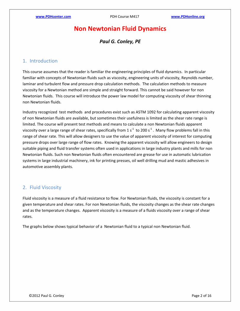
Types of Non Newtonian Fluids Rheology Models

Figure 4

There are basic 4 types of behavior for non Newtonian fluids. The first type of non Newtonian is the red line showing at a zero sear rate, there is a residual stress present at no flow. As the shear rate is increased, the shear stress increases. This curve follows the Bulkley‐Herschel model which is a power law model and is valid from shear rates of 0 up to over 1,000 s‐1. A similar case is the green line, but there is no yield stress. This is called a pure shear thinning fluid. This curve follows the power law model. The third case is a shear thickening fluid where the fluid thickens as it is sheared. The fourth case is the Bingham Plastic model where there is an initial yield stress but the curve follows a straight line as the shear rate is increased.

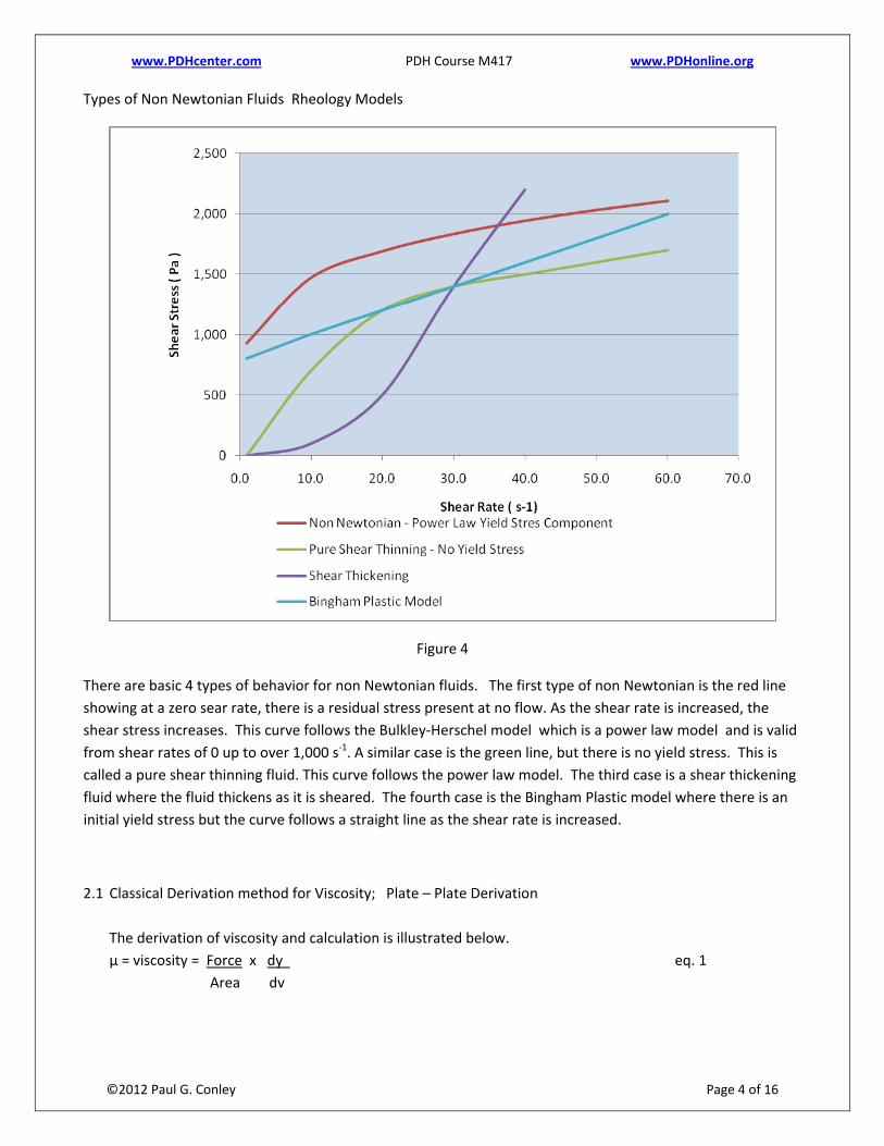
2.1 Classical Derivation method for Viscosity; Plate – Plate Derivation The derivation of viscosity and calculation is illustrated below. µ = viscosity = Force x dy eq. 1 Area dv



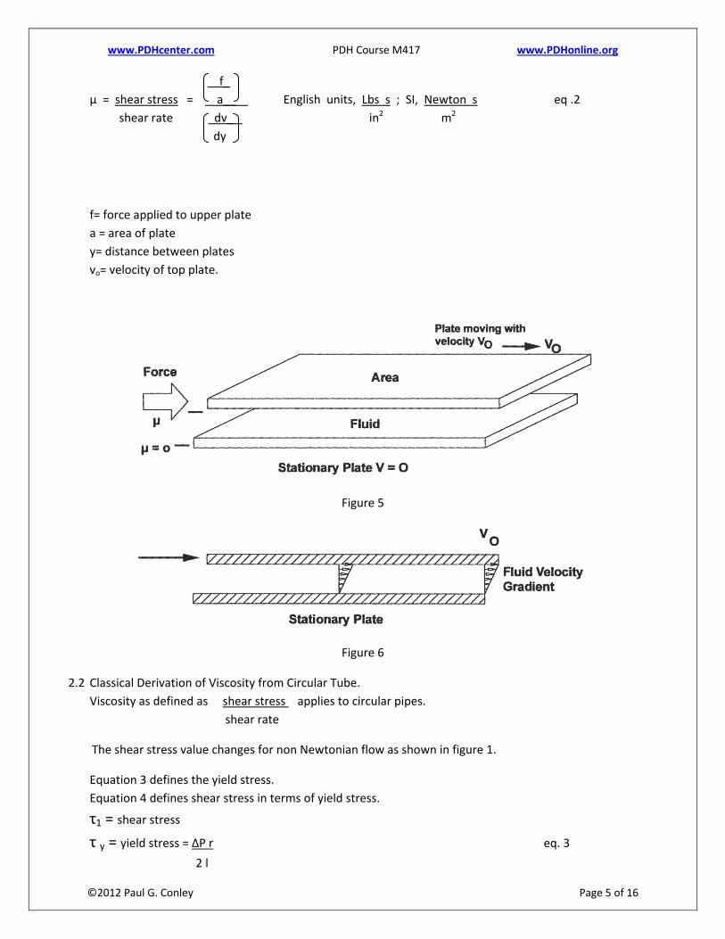
f_ µ = shear stress = a__ English units, Lbs s ; SI, Newton s eq .2 shear rate dv_ in2 m2

dy

f= force applied to upper plate a = area of plate y= distance between plates vo= velocity of top plate.

Figure 5

Figure 6

2.2 Classical Derivation of Viscosity from Circular Tube. Viscosity as defined as shear stress applies to circular pipes. shear rate

The shear stress value changes for non Newtonian flow as shown in figure 1.

Equation 3 defines the yield stress. Equation 4 defines shear stress in terms of yield stress.

τ1 = shear stress τ y = yield stress = ΔP r eq. 3 2 l



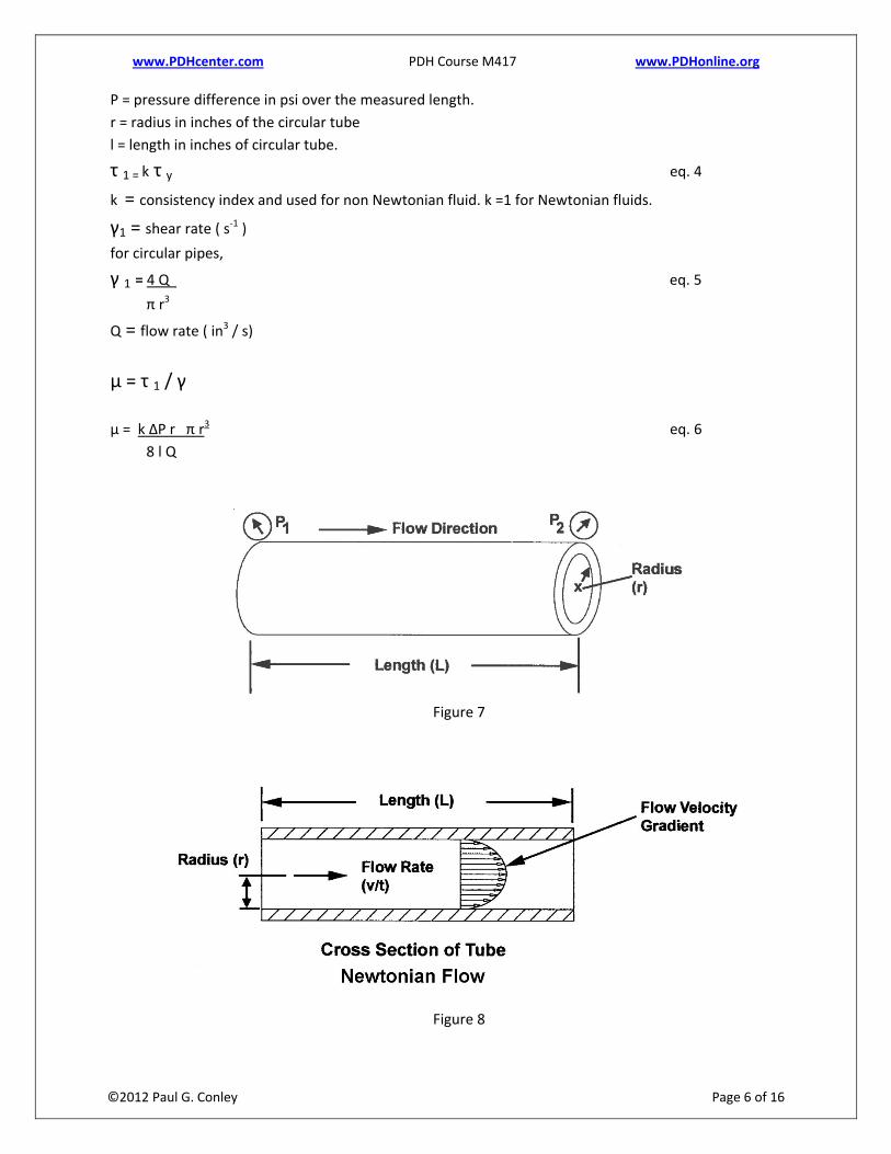
P = pressure difference in psi over the measured length. r = radius in inches of the circular tube l = length in inches of circular tube.

τ 1 = k τ y eq. 4 k = consistency index and used for non Newtonian fluid. k =1 for Newtonian fluids. γ1 = shear rate ( s‐1 ) for circular pipes,

γ 1 = 4 Q eq. 5 π r3

Q = flow rate ( in3 / s)

µ = τ 1 / γ µ = k ΔP r π r3 eq. 6 8 l Q

Figure 7

Figure 8



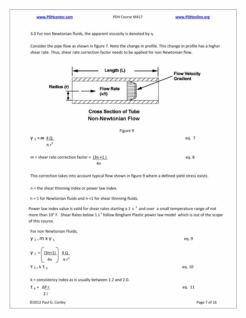
3.0 For non Newtonian fluids, the apparent viscosity is denoted by η. Consider the pipe flow as shown in figure 7. Note the change in profile. This change in profile has a higher shear rate. Thus, shear rate correction factor needs to be applied for non Newtonian flow.

Figure 9

γ 1 = m 4 Q eq. 7

π r3

m = shear rate correction factor = (3n +1 ) eq. 8 4n This correction takes into account typical flow shown in figure 9 where a defined yield stress exists. n = the shear thinning index or power law index.

n = 1 for Newtonian fluids and n <1 for shear thinning fluids.

Power law index value is valid for shear rates starting a 1 s ‐1 and over a small temperature range of not more than 10° F. Shear Rates below 1 s‐1 follow Bingham Plastic power law model which is out of the scope of this course.

For non Newtonian Fluids,

γ 1 = m x γ 1 eq. 9

γ 1 = (3n+1) 4 Q 4n π r3

τ 1 = k τ y eq. 10

k = consistency index as is usually between 1.2 and 2.0.

τ y = ΔP r eq. 11 2 l



So the value of apparent viscosity can now be expressed

η = τ 1 γ1 n‐1 eq. 12

Lets see how this all works. Because it is difficult and time consuming to generate a full apparent viscosity curve over a large shear rate range, manufactures of non Newtonian shear thinning fluids can run less complicated test to obtain the shear thinning or power law index n and the consistent index K. This can be supplied by the manufacture. In any event, in the appendix of the course, a description of equipment and test methods are presented to show how the power index and consistency index is obtained. Once these values are obtained, it is then a straight calculation as shown below to obtain pressure drops of non Newtonian fluids in circular pipes. With pressure drops known, the pump selection and the pipe wall thickness can be determined to design a safe and reliable fluid transfer system. 4.0 Some Discussion on engineering units. Like all engineering problems, units must be consistent to arrive at a correct answer. The most common presentation of viscosity is in centipoises for dynamic viscosity or centistokes for kinematic viscosity. When working in the English system, where units must break down into inch – seconds – lbs. In the SI unts, Newton ‐ meters – seconds are used. Conversion factors are needed to convert from one system of units to the other. Centistokes ( cSt ) = Centipoise / Specific Gravity Density of most fluids is such that the specific gravity is between .85 to .98. η = Centipoise ( cP ) = Centistokes x Specific Gravity For SI units of viscosity, centipoises = Pascal seconds x ( 1000 ) = Newtons s eq. 13 m2 Fore English units, absolute viscosity is reyns. η = lbs_s = Pressure ( psi ) seconds eq. 14 in2 When working in English unit and working to convert reyns to centipoises,the following Conversion factor can be used. Note the value of reyns is a small number. η Centipoise = reyns x 6,894,720



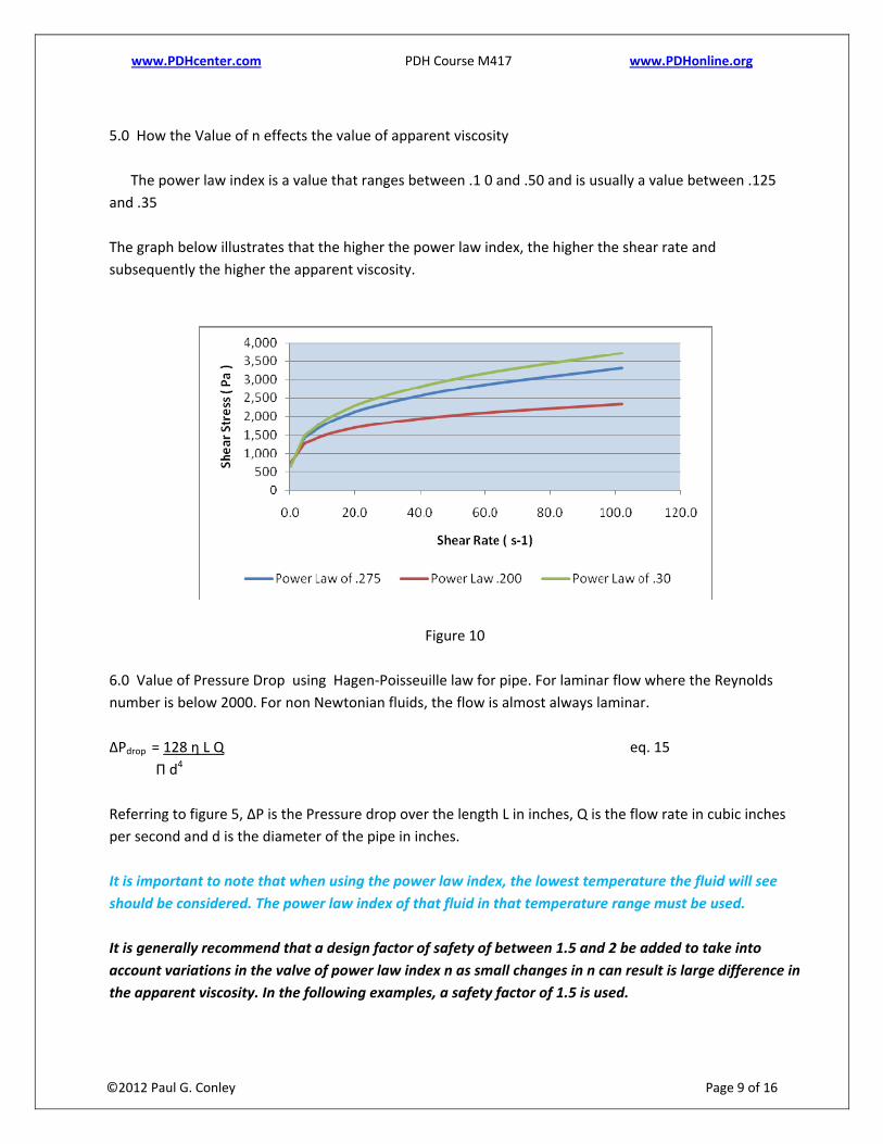
5.0 How the Value of n effects the value of apparent viscosity The power law index is a value that ranges between .1 0 and .50 and is usually a value between .125 and .35 The graph below illustrates that the higher the power law index, the higher the shear rate and subsequently the higher the apparent viscosity.

Figure 10 6.0 Value of Pressure Drop using Hagen‐Poisseuille law for pipe. For laminar flow where the Reynolds number is below 2000. For non Newtonian fluids, the flow is almost always laminar. ΔPdrop = 128 η L Q eq. 15 Π d4

Referring to figure 5, ΔP is the Pressure drop over the length L in inches, Q is the flow rate in cubic inches per second and d is the diameter of the pipe in inches. It is important to note that when using the power law index, the lowest temperature the fluid will see should be considered. The power law index of that fluid in that temperature range must be used. It is generally recommend that a design factor of safety of between 1.5 and 2 be added to take into account variations in the valve of power law index n as small changes in n can result is large difference in the apparent viscosity. In the following examples, a safety factor of 1.5 is used.



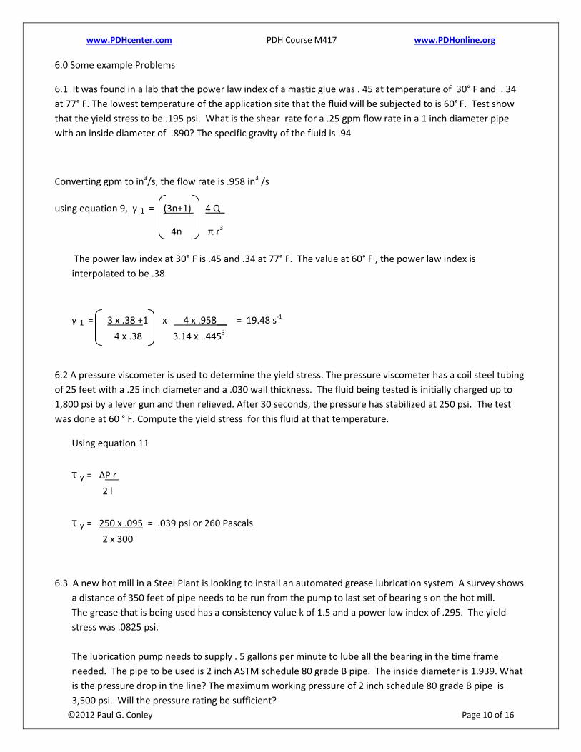
6.0 Some example Problems

6.1 It was found in a lab that the power law index of a mastic glue was . 45 at temperature of 30° F and . 34 at 77° F. The lowest temperature of the application site that the fluid will be subjected to is 60° F. Test show that the yield stress to be .195 psi. What is the shear rate for a .25 gpm flow rate in a 1 inch diameter pipe with an inside diameter of .890? The specific gravity of the fluid is .94

Converting gpm to in3/s, the flow rate is .958 in3 /s

using equation 9, γ 1 = (3n+1) 4 Q

4n π r3 The power law index at 30° F is .45 and .34 at 77° F. The value at 60° F , the power law index is interpolated to be .38

γ 1 = 3 x .38 +1 x 4 x .958__ = 19.48 s‐1

4 x .38 3.14 x .4453

6.2 A pressure viscometer is used to determine the yield stress. The pressure viscometer has a coil steel tubing of 25 feet with a .25 inch diameter and a .030 wall thickness. The fluid being tested is initially charged up to 1,800 psi by a lever gun and then relieved. After 30 seconds, the pressure has stabilized at 250 psi. The test was done at 60 ° F. Compute the yield stress for this fluid at that temperature.

Using equation 11

τ y = ΔP r 2 l

τ y = 250 x .095 = .039 psi or 260 Pascals 2 x 300

6.3 A new hot mill in a Steel Plant is looking to install an automated grease lubrication system A survey shows

a distance of 350 feet of pipe needs to be run from the pump to last set of bearing s on the hot mill. The grease that is being used has a consistency value k of 1.5 and a power law index of .295. The yield stress was .0825 psi. The lubrication pump needs to supply . 5 gallons per minute to lube all the bearing in the time frame needed. The pipe to be used is 2 inch ASTM schedule 80 grade B pipe. The inside diameter is 1.939. What is the pressure drop in the line? The maximum working pressure of 2 inch schedule 80 grade B pipe is 3,500 psi. Will the pressure rating be sufficient?



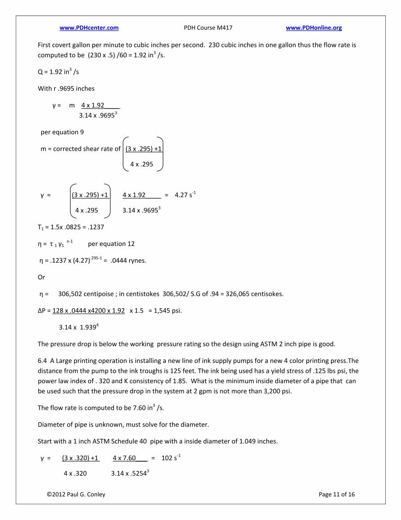
First covert gallon per minute to cubic inches per second. 230 cubic inches in one gallon thus the flow rate is computed to be (230 x .5) /60 = 1.92 in3 /s.

Q = 1.92 in3 /s

With r .9695 inches

γ = m 4 x 1.92____ 3.14 x .96953

per equation 9

m = corrected shear rate of (3 x .295) +1

4 x .295

γ = (3 x .295) +1 4 x 1.92____ = 4.27 s‐1

4 x .295 3.14 x .96953

Τ1 = 1.5x .0825 = .1237

η = τ 1 γ1 n‐1 per equation 12

η = .1237 x (4.27).295‐1 = .0444 rynes.

Or

η = 306,502 centipoise ; in centistokes 306,502/ S.G of .94 = 326,065 centisokes.

ΔP = 128 x .0444 x4200 x 1.92 x 1.5 = 1,545 psi.

3.14 x 1.9394

The pressure drop is below the working pressure rating so the design using ASTM 2 inch pipe is good.

6.4 A Large printing operation is installing a new line of ink supply pumps for a new 4 color printing press.The distance from the pump to the ink troughs is 125 feet. The ink being used has a yield stress of .125 lbs psi, the power law index of . 320 and K consistency of 1.85. What is the minimum inside diameter of a pipe that can be used such that the pressure drop in the system at 2 gpm is not more than 3,200 psi.

The flow rate is computed to be 7.60 in3 /s.

Diameter of pipe is unknown, must solve for the diameter.

Start with a 1 inch ASTM Schedule 40 pipe with a inside diameter of 1.049 inches.

γ = (3 x .320) +1 4 x 7.60___ = 102 s‐1

4 x .320 3.14 x .52543



Τ1 = 1.85 x .125 = .231

η = .231 x (102).320‐1 = .0098 rynes.

or

η = 67,979 centipoise

ΔP = 128 x .0098 x 1500 x 7.60 x 1.5 = 5,724 psi.

3.14 x 1.0494

Although the higher flow rate increases the shear rate which make a lower value for the apparent viscosity, the pressure drop is too high. A larger diameter of pipe is needed. It is up the reader to try and see what diameter minimally is needed to meet the conditions of a maximum pressure drop of less than 3,200 psi.



Appendix

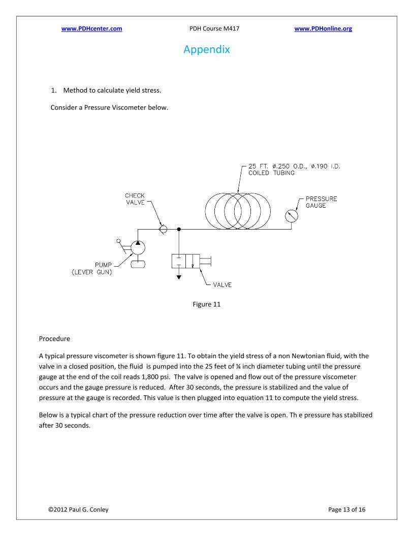
1. Method to calculate yield stress.

Consider a Pressure Viscometer below.

Figure 11

Procedure

A typical pressure viscometer is shown figure 11. To obtain the yield stress of a non Newtonian fluid, with the valve in a closed position, the fluid is pumped into the 25 feet of ¼ inch diameter tubing until the pressure gauge at the end of the coil reads 1,800 psi. The valve is opened and flow out of the pressure viscometer occurs and the gauge pressure is reduced. After 30 seconds, the pressure is stabilized and the value of pressure at the gauge is recorded. This value is then plugged into equation 11 to compute the yield stress.

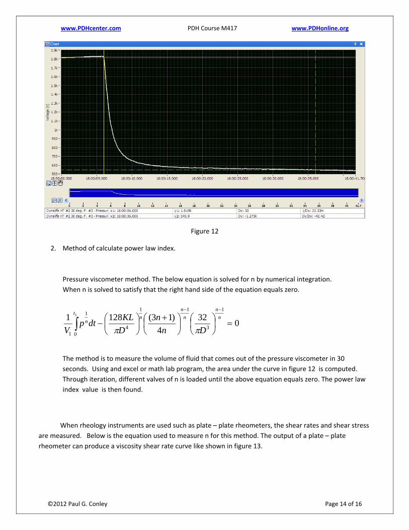
Below is a typical chart of the pressure reduction over time after the valve is open. Th e pressure has stabilized after 30 seconds.



Figure 12

2. Method of calculate power law index. Pressure viscometer method. The below equation is solved for n by numerical integration. When n is solved to satisfy that the right hand side of the equation equals zero.

0324

)13(12811

3

11

40

1

1

1

=⎟⎠⎞

⎜⎝⎛

⎟⎠⎞

⎜⎝⎛ +

⎟⎠⎞

⎜⎝⎛−

−−

∫n

nn

nn

tn

Dnn

DKLdtp

V ππ

The method is to measure the volume of fluid that comes out of the pressure viscometer in 30 seconds. Using and excel or math lab program, the area under the curve in figure 12 is computed. Through iteration, different valves of n is loaded until the above equation equals zero. The power law index value is then found.

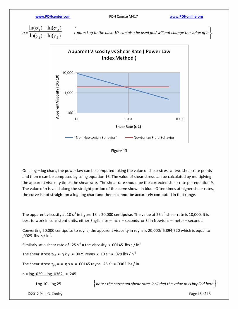
When rheology instruments are used such as plate – plate rheometers, the shear rates and shear stress are measured. Below is the equation used to measure n for this method. The output of a plate – plate rheometer can produce a viscosity shear rate curve like shown in figure 13.



n = )ln()ln()ln()ln(

21

21

γγσσ

−−

note: Log to the base 10 can also be used and will not change the value of n.

Figure 13

On a log – log chart, the power law can be computed taking the value of shear stress at two shear rate points and then n can be computed by using equation 16. The value of shear stress can be calculated by multiplying the apparent viscosity times the shear rate. The shear rate should be the corrected shear rate per equation 9. The value of n is valid along the straight portion of the curve shown in blue. Often times at higher shear rates, the curve is not straight on a log‐ log chart and then n cannot be accurately computed in that range.

The apparent viscosity at 10 s‐1 in figure 13 is 20,000 centipoise. The value at 25 s‐1 shear rate is 10,000. It is best to work in consistent units, either English lbs – inch – seconds or SI in Newtons – meter – seconds.

Converting 20,000 centipoise to reyns, the apparent viscosity in reyns is 20,000/ 6,894,720 which is equal to .0029 lbs s / in2.

Similarly at a shear rate of 25 s‐1 = the viscosity is .00145 lbs s / in2

The shear stress τ10 = η x γ = .0029 reyns x 10 s‐1 = .029 lbs /in 2

The shear stress τ25 = = η x γ = .00145 reyns 25 s‐1 = .0362 lbs / in

n = log .029 – log .0362 = .245

Log 10‐ log 25 note : the corrected shear rates included the value m is implied here



It can be noted here that the log base 10 or ln natural log will yield the same result. The value of n will be the same. The value of n will also be the same if your use centipoises to compute yield stress verse reyns as was done above.

Finally – it should be noted that n can be calculated from a shear stress vs shear rate curve per figure 1. The log of the shear stress at two shear rate points would be divided by the log of the shear rate at those points.

Check List to consider when solving problems.

1. Convert to one standard set of units. Do not mix units. Works all in English or all in SI units. 2. Flow should be converted to basic units of inches3/second or meters3/second. 3. The shear rate for non Newtonian fluids equation, the correction factor m in equation 9 must be

used. 4. You must calculate the shear stress by using valve k, consistency number and multiplying it by the

yield stress.

Some useful conversions factors

1. Reyns to Centipoise , multiply reyns by 6,894,720. ( reyns is a small number ) 2. Convert psi to Pascals, multiply psi by 6,894. 3. To convert centipoises to centistokes, divide centipoises by the specific gravity of the fluid. 4. To convert centistokes to centipoises, multiply centistokes by the specific gravity of the fluid.

Documents

Non Newtonian Fluid Dynamics - PDHonline.com · Non Newtonian Fluid Dynamics ... laminar and turbulent flow and pressure drop calculation methods. The calculation methods to measure