Ninth ARTNeT Capacity Building Workshop for Trade Research

"Trade Flows and Trade Policy Analysis"

June 2013

Bangkok, Thailand

Cosimo Beverelli and Rainer Lanz

(World Trade Organization) 1

Partial-equilibrium (PE) trade policy analysis and simulation

2

Content

a. Market access analysis with PE modelling

b. Basic PE model for analyzing welfare changes

c. Empirical tool for trade policy simulations: SMART

3

a. Market access analysis with PE modelling

4

• Rationale for market access analysis

• Rationale for PE modelling

– Advantages

– Disadvantages

b. Basic PE model for analyzing welfare changes

5

• Derivation of social welfare function

• Perfect competition

– Small open economy (SOE)

– Large country

Social welfare

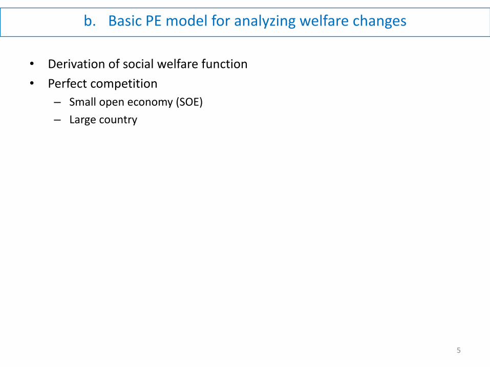
• Each consumer ℎ has quasi-linear utility function 𝑐0ℎ + 𝑈ℎ 𝑐ℎ

• Budget constraint: 𝑐0ℎ + 𝑝′𝑐ℎ ≤ 𝐼ℎ

• FOC: 1 = 𝜆 and 𝑈′ = 𝜆𝑝 = 𝑝 (demand for non-numeraire goods is independent of income)

• Demand functions are 𝑐ℎ = 𝑑ℎ 𝑝 and 𝑐0ℎ = 𝐼ℎ − 𝑝′𝑑ℎ 𝑝

• Welfare is defined as the sum of individual indirect utilities 𝑉ℎ:

𝑊 𝑝, 𝐼 ≡ 𝑉ℎ

𝐻

ℎ=1

= 𝐼ℎ − 𝑝′𝑑ℎ 𝑝 + 𝑈ℎ 𝑑ℎ 𝑝

𝐻

ℎ=1

• Notice that:

– 𝐼ℎ = 𝐼𝐻ℎ=1 (total income)

–𝜕𝑊

𝜕𝐼= 1 and (by envelope theorem)

𝜕𝑊

𝜕𝑝= −𝑑ℎ 𝑝 ≡ −𝑑 𝑝𝐻

ℎ=1

– −𝑝′𝑑ℎ 𝑝 + 𝑈ℎ 𝑑ℎ 𝑝 = 𝐶𝑆𝐻ℎ=1 (consumer surplus)

6

Social welfare (ct’d)

• To simplify, let there be only one good subject to specific tariff 𝑡

• World price is 𝑝∗ and 𝑝 = 𝑝∗ + 𝑡

• Numeraire good is freely traded at fixed world price of unity

• Labor is the only factor of production. Each unit of numeraire requires one unit of labor

– Therefore, 𝑤 = 1 and 𝑊𝐿 = 𝐿

• Output of the good subject to the tariff is 𝑦. Produced by firms with cost function 𝐶 𝑦 and marginal costs 𝐶′ 𝑦

• Imports 𝑚 = 𝑑 𝑝 − 𝑦, with 𝑑′ 𝑝 < 0

• Tariff revenue 𝑡𝑚 is redistributed to consumers

• Consumers are also entitled to profits from import-competing industry

– Under perfect competition, 𝑝𝑦 − 𝐶 𝑦 = 𝑃𝑆 (producer surplus)

– Under imperfect competition, 𝑝𝑦 − 𝐶 𝑦 = 𝜋 (industry profits)

• Social welfare is then:

𝑊 𝑝, 𝐼 = 𝑊 𝑝, 𝐿 + 𝑡𝑚 + 𝑝𝑦 − 𝐶 𝑦 ≡ 𝑊 𝑡

7

Social welfare (ct’d)

• How does social welfare vary with the tariff?

𝑑𝑊 =𝜕𝑊

𝜕𝑝 −𝑑 𝑝

𝑑𝑝 +𝜕𝑊

𝜕𝐼 =1

𝑑𝐼

𝑑𝑊 = −𝑑 𝑝 𝑑𝑝 + 𝑑 𝐿 + 𝑡𝑚 + 𝑝𝑦 − 𝐶 𝑦

𝑑𝑊 = −𝑑 𝑝 𝑑𝑝 + 𝑚𝑑𝑡 + 𝑡𝑑𝑚 + 𝑝𝑑𝑦 + 𝑦𝑑𝑝 − 𝐶′ 𝑦 𝑑𝑦

𝑑𝑊

𝑑𝑡= −𝑑 𝑝

𝑑𝑝

𝑑𝑡+ 𝑚 + 𝑡

𝑑𝑚

𝑑𝑝

𝑑𝑝

𝑑𝑡+ 𝑦

𝑑𝑝

𝑑𝑡+ 𝑝 − 𝐶′ 𝑦

𝑑𝑦

𝑑𝑡

𝑑𝑊

𝑑𝑡= 𝑡

𝑑𝑚

𝑑𝑝

𝑑𝑝

𝑑𝑡− 𝑚

𝑑𝑝∗

𝑑𝑡+ 𝑝 − 𝐶′ 𝑦

𝑑𝑦

𝑑𝑡 (1)

8

Perfect competition, SOE

• Perfect competition implies that 𝑝 = 𝐶′ 𝑦

• SOE assumption implies that 𝑑𝑝∗ 𝑑𝑡 = 0 , therefore 𝑑𝑝 = 𝑑𝑡 (there is full pass-through of the tariff to domestic price)

• Equation 1 simplifies to:

𝑑𝑊

𝑑𝑡= 𝑡

𝑑𝑚

𝑑𝑝

• Since 𝑑𝑤

𝑑𝑡 𝑡=0

= 0, the optimal tariff for a SOE is zero

9

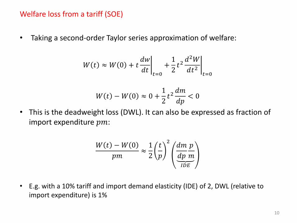
Welfare loss from a tariff (SOE)

• Taking a second-order Taylor series approximation of welfare:

𝑊 𝑡 ≈ 𝑊 0 + 𝑡𝑑𝑤

𝑑𝑡 𝑡=0

+1

2𝑡2

𝑑2𝑊

𝑑𝑡2 𝑡=0

𝑊 𝑡 − 𝑊 0 ≈ 0 +1

2𝑡2

𝑑𝑚

𝑑𝑝< 0

• This is the deadweight loss (DWL). It can also be expressed as fraction of import expenditure 𝑝𝑚:

𝑊 𝑡 − 𝑊 0

𝑝𝑚≈

1

2

𝑡

𝑝

2𝑑𝑚

𝑑𝑝

𝑝

𝑚𝐼𝐷𝐸

• E.g. with a 10% tariff and import demand elasticity (IDE) of 2, DWL (relative to import expenditure) is 1%

10

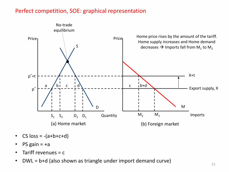
Perfect competition, SOE: graphical representation

• CS loss = -(a+b+c+d)

• PS gain = +a

• Tariff revenues = c

• DWL = b+d (also shown as triangle under import demand curve)

11

Quantity M1 Imports

Export supply, X

M

Price

M2

D

X+t p*+t

Price

S

No-trade equilibrium

Home price rises by the amount of the tariff. Home supply increases and Home demand

decreases Imports fall from M1 to M2

p*

S1 D1 S1 S2 D2

a b c d b+d

(a) Home market (b) Foreign market

c

Perfect competition, large country

• Large country assumption implies that 𝑑𝑝∗ 𝑑𝑡 ≠ 0 , therefore 𝑑𝑝 𝑑𝑡 ≠ 1

– 𝑑𝑝∗ 𝑑𝑡 < 0 (intuitively, if a large country imposes a tariff it reduces its imports sufficiently to drive down the world price

– 𝑑𝑝 𝑑𝑡 < 1 (intuitively, the pass-through of the tariff is not full, and foreign exporters absorb part of the tariff in the form of lower world price (𝑑𝑝∗ 𝑑𝑡 < 0 )

• Equation 1 becomes:

𝑑𝑊

𝑑𝑡= 𝑡

𝑑𝑚

𝑑𝑝

𝑑𝑝

𝑑𝑡= −𝑚

𝑑𝑝∗

𝑑𝑡 (2)

• Therefore: 𝑑𝑤

𝑑𝑡 𝑡=0

= −𝑚𝑑𝑝∗

𝑑𝑡> 0

• A small enough tariff will necessarily raise welfare for a large country

• What does “large” mean? 12

Optimal tariff for large country

• “Large "means that the export supply is upward sloping (i.e. elasticity of export supply is finite – vs. SOE case in which export supply is horizontal, i.e. infinitely elastic)

• Optimal tariff 𝑡𝑜𝑝𝑡 for such large country is computed where 2 equals 0:

𝑑𝑊

𝑑𝑡= 0 ⇒

𝑡𝑜𝑝𝑡

𝑝∗ = 𝑚𝑑𝑝∗

𝑑𝑡

𝑑𝑚

𝑑𝑝

𝑑𝑝

𝑑𝑡

−1

(3)

• Since domestic imports 𝑚 = foreign exports 𝑥, 𝑑𝑚

𝑑𝑝

𝑑𝑝

𝑑𝑡=

𝑑𝑥

𝑑𝑡. Therefore:

𝑡𝑜𝑝𝑡

𝑝∗=

𝑑𝑥

𝑑𝑝∗

𝑝∗

𝑥𝑋𝑆𝐸

−1

4

• Optimal % tariff is equal to the inverse of the export supply elasticity (XSE)

13

Optimal tariff for large country (ct’d)

• Alternatively, equation 4 can be re-arranged to yield:

𝑡𝑜𝑝𝑡

𝑝=

𝑑𝑚

𝑑𝑝

𝑝

𝑚𝐼𝐷𝐸

−1𝑑𝑝∗ 𝑑𝑡

𝑑𝑝 𝑑𝑡

• Optimal % tariff is larger:

– the smaller the pass-through 𝑑𝑝 𝑑𝑡

– ⇔ the larger the terms-of-trade (TOT) gain 𝑑𝑝∗ 𝑑𝑡

14

Optimal tariff for large country: graphical representation

• The increase in the domestic price is less than the tariff (𝑑𝑝 𝑑𝑡 < 1)

• Foreign exporters absorb part of the tariff (𝑑𝑝∗ 𝑑𝑡 < 0): area “e” = TOT gain

• If the gain of e is greater than the DWL loss (b+d), Home gains

15

A

Price

a c P*+t

p0

p*

S

b d

Price

Imports

e D

S1 S2 D2 D1 Quantity M2 M1

M

X+t

e

X

B*

C

C*

b+d

No-trade equilibrium

t

(a) Home market (b) Foreign market

c

Empirical evidence

• Broda et al. (2008) find that prior to WTO membership, countries set import tariffs 9 percentage points higher on inelastically supplied imports relative to those supplied elastically

• See bonus exercise for a replication of their results

• See also the R. Feenstra, “Advanced International Trade” (Princeton, 2004), Chapter 7, Section “Tariffs on Japanese Trucks and Motorcycles” (pp. 233-240).

16

c. Empirical tool for trade policy simulations: SMART

17

• Chapter 4 of the Practical Guide to TPA discusses various empirical tools

• Here we use SMART (built-in in WITS)

SMART

• Overview

• Theoretical underpinnings

– Export supply side

– Demand side

• Effects of policy changes

– Trade effects

– Effects on Tariff Revenue, Consumer Surplus and Welfare

• More details and formulas in Jammes and Olarreaga (2005)

SMART example: Albania’s unilateral trade liberalization with the EU

• In 2007, Albania sourced buses (HS 870210) from 19 trading partners, of which 11 were European Union countries

• Albania levied tariffs from all sources, including the EU

• Using SMART, the user can simulate the effect of a full trade liberalization towards the EU, but not to the rest of the world

• SMART yields the results that all 11 EU countries would be able to increase their exports to Albania, for example Germany, the biggest exporter, by almost 1 million USD

• Non-EU countries, by contrast, would see their shares shrink, in particular the US, by about 0.3 million USD

• SMART results indicate that the tariff liberalization would:

– Increase imports

– Lower tariff revenues

– Raise consumer surplus (Albania is a SOE)

• Results in this folder

18