NOAA Technical Report NOS NGS 62

Blueprint for the Modernized NSRS, Part 1: Geometric Coordinates and Terrestrial Reference Frames

April 2017 Revised April 2021 Silver Spring, MD

ii

Versions Date Changes April 28, 2017

Original Release

September 21, 2017

This versions page was added Author list removed from front cover Acknowledgements section added “PTRF2022” changed to “PATRF2022” “CTRF2022” changed to “CATRF2022” “MTRF2022” changed to “MATRF2022” “GRS-80” changed to “GRS 80” Minor typographical errors were corrected

April 20, 2021

Changes from the last version: • An official delay was announced• Attempts to remove all “TBDs” were made• Adoption of ITRF2020 • Pre-eminence of XYZ, over φλh, as definitive coordinates• Decision to propagate EPP2022 errors into *TRF2022 coordinates has been

reversed. EPP2022 will be treated as a fixed conventional set of values, not unlike GRS 80

• The official definitional relationship between ITRF2020 and the *TRF2022 frames has been changed from the complicated M-1(θ0, λ0, �̇�𝜔0, t, t0) matrix toa much simpler R(�̇�𝜔𝑋𝑋, �̇�𝜔𝑌𝑌, �̇�𝜔𝑍𝑍, t, t0) matrix

• Much of the derivational part of the report, previously in chapters 5 and 7 have been moved to Appendix A and re-written for clarity

• The term Intra-frame Velocity Model (IFVM) has been flagged as “preliminary”, with the word “Velocity” under consideration for replacement in the future.

• A discussion of new coordinate types is provided• An acronym, abbreviation and initialism list is provided• A section on updating vs replacing the frames is added• A new figure showing GIA velocities was added

iii

Contents Acknowledgements from the 2021 version ............................................................................. v

Acknowledgements from the 2017 version ............................................................................. v

Delayed Release of the Modernized NSRS .............................................................................. vi

Executive Summary............................................................................................................... vii

List of Abbreviations, Acronyms and Initialisms ..................................................................... viii

1 Purpose ........................................................................................................................... 1

2 Introduction..................................................................................................................... 1

3 “Geodetic Control”........................................................................................................... 2

3.1 International Geodetic Control Activities .................................................................... 4

3.2 National Geodetic Control Activities ........................................................................... 6

3.2.1 NOAA Foundation CORS Network (NFCN) ............................................................ 7

4 “Plate-Fixed” Frames and Euler Poles ............................................................................... 7

5 ITRF versus Plate-Fixed Frames........................................................................................15

6 The Modernized Reference Frames .................................................................................16

7 Intra-Frame Velocities .....................................................................................................18

8 Types of Coordinates.......................................................................................................22

8.1 Coordinate Functions ................................................................................................23

8.2 Survey Epoch Coordinates.........................................................................................24

8.3 Reference Epoch Coordinates ...................................................................................25

8.4 Projected Coordinates ..............................................................................................25

8.4.1 State Plane Coordinate System (SPCS) ................................................................26

8.4.2 Universal Transverse Mercator (UTM) ................................................................26

8.4.3 U.S. National Grid (USNG) ..................................................................................26

9 Relating Coordinates across Frames and Epochs ..............................................................26

10 Updating and Replacing the Four Terrestrial Reference Frames ........................................28

10.1 Updating the Reference Frames and Their Associated Components........................28

10.2 Drivers of Updates.................................................................................................30

10.2.1 New Versions of the ITRF ...................................................................................31

10.3 Replacing the Terrestrial Reference Frames ...........................................................31

iv

11 Summary ........................................................................................................................32

12 Bibliography....................................................................................................................32

Appendix A: Euler Pole Parameters .........................................................................................34

Relationship between an Ideal Frame and a Plate Fixed Frame.............................................34

Considering a Simplified M-1 Matrix .....................................................................................43

Using Three rotation Rates Rather Than (Co-)Latitude, Longitude and Rotation Rate as the Euler Pole Parameters.........................................................................................................45

Computing the Rotations ....................................................................................................51

v

Acknowledgements from the 2021 version The following people deserve thanks for their contributions to this updated document:

Michael Craymer (CGS), Jacob Heck, Jeff Jalbrzikowski, Dan Roman, Jarir Saleh, Brian Shaw, Dru Smith, Bill Stone, Dave Zenk

Acknowledgements from the 2017 version A work of this magnitude requires the input of many people. The contents of this document grew out of a long list of scientific meetings inside NGS, beginning in 2014, which grew in scope and frequency through 2015 and 2016. Many scientists inside NGS and eventually outside of NGS contributed to the conversations that ultimately led to this document. Recognition and thanks for their contributions should go to the following individuals (in alphabetic order):

Mark Armstrong, Dana Caccamise, Kevin Choi, Mike Cline, Michael Craymer (GSC), Michael Dennis, Joe Evjen, Pam Fromhertz, Daniel Gillins, Steve Hilla, Nic Kinsman, Gerry Mader, Julie Prusky, Dan Roman, Jarir Saleh, Mark Schenewerk, Giovanni Sella, Dru Smith, Tomas Soler, Bill Stone, Neil Weston, Sungpil Yoon

vi

Delayed Release of the Modernized NSRS NOAA’s National Geodetic Survey (NGS) is announcing a delay in the release of the modernized National Spatial Reference System (NSRS). In 2007, NGS began planning for the modernized NSRS, acquiring its first airborne gravimeter, creating and initiating the GRAV-D project and by 2008 had codified its modernization plans into a Ten Year Plan. At that time, the target completion date was 2018. By 2013, that date seemed unlikely, due to both the broadening of the Gravity for the Redefinition of the American Vertical Datum (GRAV-D) coverage area and the experience of five years of operational planning and execution. In 2013, NGS revised its 2007 Strategic Plan, and targeted 2022 as the date of the release of the modernized NSRS. This date was reinforced with a 2018 Strategic Plan revision. By 2017, confidence in hitting the 2022 target was high enough to reach final agreement with Canada and Mexico on a naming convention for certain components, to include “2022” in their names. Since 2017, operational, workforce, and other issues have arisen and compounded, causing NGS to recently re-evaluate whether a successful roll-out by 2022 is possible. The most significant impacts have been in workforce hiring and retention, and in meeting GRAV-D data collection milestones, which underpin the NSRS modernization efforts. NGS is currently conducting a comprehensive analysis of ongoing projects, programs, and resources required to complete NSRS modernization and will continue to provide regular updates on our progress. To get the latest news on NSRS modernization and track our progress, subscribe to NGS News or visit our "New Datums" web pages.

vii

Executive Summary NOAA Technical Report NOS NGS 62

Blueprint for the Modernized NSRS, Part 1: Geometric Coordinates and Terrestrial Reference Frames

In the next few years, the entire National Spatial Reference System (NSRS) will be modernized. This document addresses the geometric aspects of the NSRS. Geometrically, the NSRS currently contains three reference frames (historically “horizontal datums”), known as NAD 83 (2011), NAD 83 (PA11), and NAD 83 (MA11) that are used to define the geodetic latitudes, geodetic longitudes, and ellipsoidal heights of all points in the USA. These three frames will be replaced with four new plate-fixed reference frames, called:

• North American Terrestrial Reference Frame of 2022 (NATRF2022) • Pacific Terrestrial Reference Frame of 2022 (PATRF2022) • Caribbean Terrestrial Reference Frame of 2022 (CATRF2022) • Mariana Terrestrial Reference Frame of 2022 (MATRF2022)

The time-dependent Cartesian coordinate of any point on Earth in any of these four plate-fixed frames will be defined relative to the time-dependent Cartesian coordinates in ITRF2020. The relative relationship will rely on a plate rotation model for each tectonic plate associated with each frame. This relationship will rely on rotations about the three ITRF axes (called Euler pole parameters, or EPPs), and be codified in a model called EPP2022. Such time-dependent coordinates will exhibit coordinate stability in areas of the continent where motion of the tectonic plate is fully characterized by plate rotation. All remaining velocities (including horizontal motions induced directly or indirectly by adjoining tectonic plates, horizontal motions induced by glacial isostatic adjustment, other horizontal motions and all vertical motions in their entirety) will be captured by a model, tentatively called an Intra-Frame Velocity Model (IFVM) and tentatively named IFVM2022. NGS will build all modernized geometric tools to work in Cartesian ITRF2020 coordinates. But with EPP2022 (used to change frames) and IFVM2022 (used to change epochs), NGS will provide users with adjusted coordinates in other frames and at user-needed epochs. The ellipsoid used to relate Cartesian coordinates to geodetic coordinates will be GRS 80.

viii

List of Abbreviations, Acronyms and Initialisms AC Active Coordinate (NGS); Analysis Center (IGS)

APREF Asia-Pacific Reference Frame

CATRF2022 Caribbean Terrestrial Reference Frame of 2022

CGS Canadian Geodetic Survey

CORS Continuously Operating (GNSS) Reference Station

DORIS Doppler Orbitography by Radiopositioning Integrated on Satellite

ECEF Earth-Centered, Earth-Fixed (Cartesian coordinates)

EPP Euler Pole Parameter

FEMA Federal Emergency Management Agency

GDA Geospatial Data Act of 2018

GNSS Global Navigation Satellite System

GPS Global Positioning System

GRS 80 Geodetic Reference System of 1980

HTDP Horizontal Time Dependent Positioning (NGS software)

IAG International Association of Geodesy

IDB See NGS IDB

IERS International Earth Rotation and Reference Systems Service

IGS International GNSS Service

IFVM Intra-frame Velocity Model

IFVM2022 Intra-frame Velocity Model of 2022IGS

ITRF International Terrestrial Reference Frame

MATRF2022 Mariana Terrestrial Reference Frame of 2022

NAD 83 North American Datum of 1983

NADCON North American Datum CONversion (NGS software)

NASA National Aeronautics and Space Administration

NATRF2022 North American Terrestrial Reference Frame of 2022

NCAT NGS Coordinate Conversion and Transformation Tool (NGS software)

NCN NOAA CORS Network

NFCN NOAA Foundation CORS Network

ix

NGA National Geospatial-Intelligence Agency

NGS National Geodetic Survey

NGS IDB National Geodetic Survey Integrated Database (alternatively NGSIDB)

NOAA National Oceanic and Atmospheric Administration

NSRS National Spatial Reference System

NSRS DB National Spatial Reference System Database

OMB Office of Management and Budget

OPUS Online Positioning User Service (NGS software)

PATRF2022 Pacific Terrestrial Reference Frame of 2022

REC Reference Epoch Coordinate

RTK Real-Time Kinematic

RTN Real-Time Network

SEC Survey Epoch Coordinate

SIRGAS Sistema de Referencia Geocéntrico para Las Américas

SLR Satellite Laser Ranging

SPCS2022 State Plane Coordinate System of 2022

TRF Terrestrial Reference Frame

USACE United States Army Corps of Engineers

USGS United States Geological Survey

VLBI Very Long Baseline Interferometry

1

1 Purpose The intent of this document is to provide to the public the current status of plans by the National Geodetic Survey (NGS) to modernize the National Spatial Reference System (NSRS). This particular document covers the Geometric component; that is, the definition and determination of latitude, longitude, and ellipsoidal heights, and the terrestrial reference frames within which those values will be defined. This document attempts to be comprehensive, without being unduly lengthy. Once the fully modernized NSRS has been released, a separate report will be issued by NGS describing its creation and serving also as an “as built” description.

2 Introduction The mission of the NGS is to define, maintain, and provide access to the NSRS, to meet our nation’s economic, social, and environmental needs. The NSRS is defined by the Office of Management and Budget’s (OMB) Circular A-16 (Coordination of Geographic Information and Related Spatial Data Activities) as “the fundamental geodetic control for the United States” and is required to be used by all federal government agencies creating geographic information within the United States1. In fact, the NSRS is also the primary spatial reference framework in the nation for geospatial activities undertaken by regional, state, and local governments, many private sector organizations, and academia. Datums / reference frames are an essential component for geospatial data, serving as the foundation to help align geospatial data from disparate sources. When performing analysis with geospatial data, using a consistent datum or reference frame assures that different datasets are correctly referenced to one another and decisions made from this analysis are accurate. Consistency in coordinates is a fundamental reason the OMB Circular A-16 mandates federal agencies to use the NSRS to eliminate the significant effort that would be needed if different agencies use different datums and reference frames. Similar to how the concrete foundation

1 In 2018 a new law, the Geospatial Data Act (GDA) was passed that re-defined parts of OMB A-16 while leaving other parts unaddressed. One of the parts left unaddressed was the NSRS and geodetic control in general. A cross-agency working group continues to work on interpretation and implementation between GDA and OMB A-16. Based on that working group’s guidance, NGS’s role and authority as per OMB A-16 remains intact.

2

helps to keep the frame of a house in place, datums and reference frames help to keep geospatial data properly aligned. In order to keep up with changing technology and improved accuracy, NGS has planned for a modernization of the NSRS, originally set for 2022 but now slightly delayed (see delay message at beginning of this report). In order that this modernization maintains the usefulness of the NSRS, the function of geodetic control should be clearly articulated first.

3 “Geodetic Control” According to OMB A-16, “geodetic control provides a common reference system for establishing coordinates for all geographic data.” That is, geodetic control is some system that allows users to determine the latitude, longitude, height, gravity or other coordinate at points in their geographic dataset in such a way that these coordinates are consistent with similarly derived coordinates prepared by other users using other datasets, but using the same geodetic control. Therefore, the geodetic control must be more accurate than any map or other data set built using it. Unfortunately missing from this functional statement is the reality that geodetic control points (and their respective coordinates) can, and do, move over time. A significant portion of this blueprint will be dedicated to addressing why this is true and what can be done about it. To fulfill its function, classical geodetic control was usually a network of metal disks or rods affixed to the surface of the Earth with some associated coordinates such as latitude, longitude, height, or gravity, and where such coordinates are mutually consistent within the network. Such points served as “starting points” for the users of geodetic control to begin their own surveys and thus create their own maps or other geographic datasets. By requiring all federal 2 creators of geographic data to use the same geodetic control network (the NSRS), all geographic data in the United States created at the federal level should therefore be mutually consistent. As technology has progressed, the ability to establish accurate positions has outpaced the accuracy of the underlying geodetic infrastructure. Coordinates change over time due to a variety of factors operating over different spatial and temporal scales. In general, these

2 Non-military, non-intelligence agencies. Geodetic control for those agencies, when used outside of the United States, is the mission of the National Geospatial-Intelligence Agency (NGA)

3

coordinate changes were either spatially small or temporally very long, and were of a magnitude smaller than the accuracy of the surveys that created the coordinates. Therefore, it was possible for geodetic control to function for decades with the assumption of “fixed” coordinates, only occasionally getting updated in certain locations when movement, exceeding the accuracy of existing surveys, was finally detected. That all changed in the 1980s with the advent of the Global Positioning System (GPS) and later other space-based geodetic techniques. These new positioning technologies, with their ability to measure very long baselines to a few centimeters of accuracy, began to detect (and thus validate the theory of) plate tectonics. In addition to facilitating scientific discovery and furthering our understanding of the dynamic nature of Earth, the GPS era has also rendered deficient certain aspects of existing, convention-ally established geodetic infrastructure. GPS use by geospatial professionals such as surveyors and engineers ushered in a measurement tool with an accuracy capable of detecting change to geodetic control points and that often exceeded the accuracy of the underlying geodetic infra-structure. In consideration of the impact of plate tectonics — and other geophysical processes — on the development and use of geodetic control, a variety of approaches have been attempted in recent decades. Generally speaking, a primary consideration in determining an optimal approach is the geographic area of interest served by that control, particularly whether global or regional/national in scope, and the types of applications that will be supported. No one methodology is optimized for all uses, and this document will focus on two approaches, both of which play a role in the modernized NSRS:

1) Global, plate-independent reference frames, such as the International Terrestrial Reference Frame (ITRF), which embrace time dependency as part of geodetic control; and 2) “Plate-Fixed Frames,” such as the North American Datum of 1983 (NAD 83), which attempt to “affix” a coordinate frame (at least in latitude and longitude) to one tectonic plate in an attempt to maintain unchanging or minimally changing coordinates on that plate.

Also, regardless of how tectonic plate motion is addressed in the development of a reference frame, the purpose of geodetic control is to provide starting points by which geospatial users can define positions with the consistency and reliability of the NSRS. Such starting points should have known coordinates at an epoch that is useful to the geospatial professionals using the control. If those coordinates have changed over time, then it would be convenient and useful if

4

some component of the geodetic control would allow for comparison of previously determined geospatial coordinates at different epochs. This temporal aspect of geodetic control will play an integral role in the modernized NSRS.

3.1 International Geodetic Control Activities The NGS mission to provide the NSRS encompasses only United States’ areas of interest3. Until the 20th century, most geodetic control activities around the world were carried out by individual nations for their specific needs, with little international coordination4. That began to change in the late 20th century, with the advent of GPS and other space geodetic techniques. However, fundamental aspects of modern geodetic infrastructure and technologies, particularly space-based ones, are inherently global in nature. Accordingly, NGS engages in international geodetic technical and organizational initiatives to ensure a rigorous connection among the national and global positioning frameworks and to facilitate the use of global models, data, and products. This relationship plays a definitional role in the modernized NSRS paradigm; it is the connection that allows geospatial professionals to reap advantages on both scales — nationally and globally. Because the modernized NSRS will rely upon international cooperative activities more than ever before, a few words about the current state of these activities is warranted. The International Earth Rotation and Reference System Service (IERS) produces the International Terrestrial Reference Frame (ITRF), a global plate-independent reference frame. The ITRF is created through the collaboration of geodetic organizations worldwide that contribute data and products derived from four space geodesy techniques — Global Navigation Satellite Systems (GNSS), Very Long Baseline Interferometry (VLBI), Satellite Laser Ranging (SLR), and Doppler Orbitography and Radiopositioning Integrated by Satellite (DORIS). Data from each of these techniques is collected through four services of the International Association of Geodesy (IAG), and these services each produce a technique-specific solution of the global reference frame. The IERS then combines the four solutions to realize the ITRF, as a multi-technique global frame of the highest accuracy possible. Multiple ITRFs have been produced since 1988, with the most recent being ITRF2014. According to the IAG Global Geodetic Observing System (GGOS) requirements (Plag and Pearlman, 2009), the ITRF is intended to be accurate to 1.0 mm with stability measured at 0.1 mm/year.

3 However, much of the modernized NSRS will encompass, and be available for use by, neighboring countries; in particular most countries in North America, Central America and the Caribbean. 4 One notable exception has been the coordination between the USA and Canada, on NAD 27 and continuing into NAD 83.

5

One of the four services mentioned above, the International GNSS Service (IGS), coordinates the GNSS contribution to the ITRF, through several IGS Analysis Centers (AC), of which NGS is one. ACs process worldwide GNSS observation data to estimate station coordinate and velocity functions and to produce high accuracy GNSS satellite orbits. The IGS then combines the individual AC solutions into final products that in turn contribute to the ITRF and are utilized directly in positioning and research applications around the world, including in various NGS products and services. The current realization of the IGS reference frame is IGS145 (Rebischung and Schmid, 2016). A brief word about the difference between the reference frames produced by the IGS (such as IGS14 and IGb14) and the IERS (such as ITRF2014) is also warranted. While the IGS submits only one type of geodetic data (GNSS) of the four types that generate the ITRF, these same data are also used by the IGS to create their own GNSS-only global plate-independent reference frame. The IGS frames use more up to date antenna calibration models that affect the determination of the absolute coordinates of the IGS stations, but the IGS frames are precisely aligned to the ITRF so that the differences between the two frames are only point specific. Therefore, while there are small differences between the frames created by the IGS and the IERS, these differences are also tracked and accounted for within the international geodetic community. To most professional users of NGS products and services, no discernable difference between coordinates computed in an IGS frame or an IERS frame should be observed. Therefore NGS has decided, for the simplest communication with the public in most products and services (such as OPUS), to label global plate-independent coordinates as being in the “ITRF” unless there is some explicit reason not to do so. The modernized NSRS will contain four plate-fixed frames, and the determination of the EPPs for each of those frames will require critical international collaborations. For example, for the North American EPPs, efforts are ongoing within a working group under the IAG Regional Subcommission 1.3c (Regional Reference Frames for North America). Similar efforts exist for the Caribbean plate (Sistema de Referencia Geocéntrico para Las Américas, or SIRGAS, Working Group 1; equivalent to IAG Regional Subcommission 1.3b) and the Pacific plate (Asia-Pacific Reference Frame, or APREF, project; equivalent to IAG Subcommission 1.3e) Finally, it should be noted that the ITRF is truly global in nature but is frequently implemented regionally. While it may seem that NGS is providing its own definition of the ITRF, NGS is

5 A minor update to IGS14, called IGb14 was issued during the writing of this document. Details can be found at https://lists.igs.org/pipermail/igsmail/2020/007917.html

6

actually working in the ITRF. The Sistema de Referencia Geocéntrico para las Américas (SIRGAS) and the Asia-Pacific Reference Frame (APREF) are two reference frame endeavors with which the U.S. participates. SIRGAS, a geocentric reference system, is defined as identical to the International Terrestrial Reference System (ITRS). Its realization is a regional densification of the global International Terrestrial Reference Frame (ITRF) in Latin America and the Caribbean. By agreement within the United Nations Regional Committee for Global Information Management for the Americas (UN-GGIM-Americas), the SIRGAS reference frame is adopted for all countries within the Americas including the United States and Canada. The U.S. actively participates in SIRGAS to ensure that the realization of SIRGAS in CONUS, Alaska, Puerto Rico, and the U.S. Virgin Islands is consistent with plans for the modernized NSRS. Coordination with other countries in SIRGAS is necessary to effectively realize the modernized NSRS terrestrial reference frames on both the North American and Caribbean plates. Similarly, coordination with APREF is necessary to realize the modernized NSRS frames on the Pacific and Mariana plates. The intent of this collaboration is to ensure that the modernized NSRS is consistent with the ITRF and accessible by other nations that might lie within the regions covered by NSRS. This will enable those nations that choose to use NGS products and services to generate data consistent with the NSRS and better enable data assimilation for broader purposes (e.g., weather/ocean observations from all sources for hurricane monitoring). As a summary comparison — if the modernized NSRS is the foundation for all geospatial activities in the United States, then the ITRF is the foundation of the modernized NSRS. This important relationship will be explored later in this document.

3.2 National Geodetic Control Activities Until the late 20th century, the national geodetic infrastructure (what is now called the NSRS) was predominantly a continental effort, geared toward the needs of North American countries (specifically Canada and the USA). For example, the ellipsoid used in the North American Datum of 1927 (NAD 27) was positioned to fit to the North American continent, not the Earth. When the North American Datum of 1983 (NAD 83) was originally defined, it relied upon mostly terrestrial data collected in the United States, Canada, Mexico, and the Caribbean, augmented with a small amount of global data (such as Doppler) in order to best fit the datum to the Earth (Schwarz, et al, 1989). Shortly afterwards, however, a more direct effort evolved to relate NAD 83 to the international framework, specifically the newly defined ITRF88. This evolution of NAD 83 was further facilitated, in part, by activities such as the statewide High Accuracy Reference Networks (HARNs), developed to provide an updated datum realization consistent with GPS.

7

Additionally, the type of geodetic control that serves as the backbone of the NSRS has changed in recent decades. With the rise of various global navigation satellite systems (GNSSs), such as the U.S. Global Positioning System (GPS), NGS has relied less upon infrequently surveyed marks (so-called “passive control”) and more upon continuously operating GNSS reference stations (so-called “active control”) generically called cGNSS stations (for continuous GNSS), though usually referred to as Continuously Operating Reference Stations (CORSs). Those CORSs that are managed by NGS are known as the NOAA CORS Network (NCN). NCN stations across the nation provide the primary realization and user-access of the NSRS through GNSS observation data, published station coordinates and velocity functions, and ancillary station data. It is at these CORSs where the abstract notion of a terrestrial reference frame becomes concrete and accessible through GNSS observation data and related information. Data from the NCN also contribute to the development of the ITRF, thereby providing a direct linkage between the national and global frameworks. This relationship — which plays a vital role in the NSRS modernization — will be further explored later in this document.

3.2.1 NOAA Foundation CORS Network (NFCN) If the NCN is the backbone of the NSRS, then the backbone of the NCN is the NOAA Foundation CORS Network (NFCN), which forms a subset of the larger NCN. These Foundation CORSs (FCORSs) will also be submitted to the IGS to become IGS stations, thereby ensuring a solid link between the ITRF and the NSRS. A bulk of the NFCN are stations where other space-based techniques are collocated (e.g., VLBI, SLR, DORIS) and are critical to the definition of the ITRF. These stations will be part of the NCN and the IGS Network. Further, these stations help the IGS to define and maintain the IGS reference frame.

4 “Plate-Fixed” Frames and Euler Poles It was only a century ago that “continental drift” was first proposed (Wegener, 1915), but it wasn’t until the 1950s that enough evidence of “plate tectonics” began to accumulate that in the 1970s it became an accepted, proven theory. Today, it is recognized that the motion of many plates is not best characterized by “drift,” but rather could be more accurately described as “rotation.” When considering only the rigid (not deforming) part of a tectonic plate, the horizontal motion of the plate (relative to a global plate-independent reference frame, like the ITRF) can be modeled as a rotation about a geocentric axis passing through a fixed point on Earth’s surface. Although such models must make certain assumptions (such as the rigidity of

8

the plate), the dominant motion of the majority of points on most tectonic plates is the rotation about a fixed point. That point is known as an “Euler pole.” See Figure 1. The determination of a plate’s Euler Pole location and the angular velocity with which the plate rotates can be empirically determined through the analysis of years (or decades) of GNSS observations distributed throughout the plate. With longer time series, wider geographic distribution of observations, and the accurate modeling of non-Eulerian motions, the knowledge of the plate’s rotation improves. Under the presumption that plate-wide small (relative) magnitude horizontal motions like that from glacial isostatic adjustment (GIA) are properly modeled and removed from the otherwise rigid parts of a tectonic plate, the plate can be assumed to have effectively non-deforming (rigid) portions. These portions of the plate are generally in the interior, and if this part of the plate is truly rigid, points therein do not move relative to one another. This discussion is restricted solely to these rigid portions. The Euler pole of any given plate may or may not be on the plate itself, but the location of that pole, and the rotation about it are usually treated as constant (often expressed in angular velocity units such as degrees of rotation per million years or milli-arc-radians per year). This means that, viewed from a purely horizontal motion standpoint, points nearer the Euler pole seem to be moving slower and points further from the Euler pole appear to be moving faster but they are all moving at the same angular velocity.

9

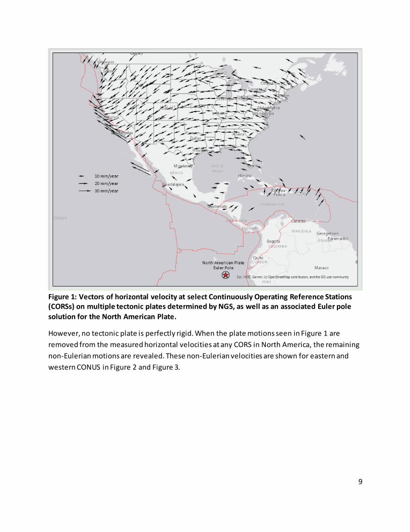
Figure 1: Vectors of horizontal velocity at select Continuously Operating Reference Stations (CORSs) on multiple tectonic plates determined by NGS, as well as an associated Euler pole solution for the North American Plate.

However, no tectonic plate is perfectly rigid. When the plate motions seen in Figure 1 are removed from the measured horizontal velocities at any CORS in North America, the remaining non-Eulerian motions are revealed. These non-Eulerian velocities are shown for eastern and western CONUS in Figure 2 and Figure 3.

10

Figure 2: Horizontal non-Eulerian velocities (observed minus Euler-derived) to the east of longitude 250°. Their magnitude is smaller than 2 mm/year. It is expected that those stations which were used to derive the Euler pole will behave well (have small non-Eulerian velocities) while other stations may have larger non-Eulerian velocities.

11

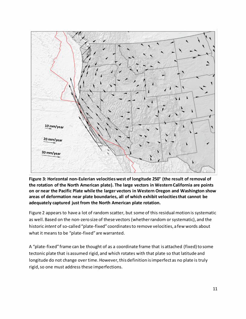
Figure 3: Horizontal non-Eulerian velocities west of longitude 250° (the result of removal of the rotation of the North American plate). The large vectors in Western California are points on or near the Pacific Plate while the larger vectors in Western Oregon and Washington show areas of deformation near plate boundaries, all of which exhibit velocities that cannot be adequately captured just from the North American plate rotation.

Figure 2 appears to have a lot of random scatter, but some of this residual motion is systematic as well. Based on the non-zero size of these vectors (whether random or systematic), and the historic intent of so-called “plate-fixed” coordinates to remove velocities, a few words about what it means to be “plate-fixed” are warranted. A “plate-fixed” frame can be thought of as a coordinate frame that is attached (fixed) to some tectonic plate that is assumed rigid, and which rotates with that plate so that latitude and longitude do not change over time. However, this definition is imperfect as no plate is truly rigid, so one must address these imperfections.

12

First, the statement that tectonic plates rotate is true but slightly misleading. It is far more accurate to say that tectonic plates are both rotating and internally deforming. Once those two behaviors are considered, one must immediately ask how to separate them from one another, whether to separate them from one another, and whether these questions even make sense. Looking at Figure 1, one might infer a rotational pattern, but Figure 2 indicates that the removal of a “best fit rotation” does not remove all changes to latitude and longitude in time. In fact, a careful look at Figure 2 shows that a systematic deformation (most stations moving toward Hudson Bay) was left behind. This motion is due to Glacial Isostatic Adjustment (GIA) related to the last ice and centered on Hudson Bay. One such model of this motion is seen in Figure 4 and Figure 5. One may view this deformation as either information or a nuisance. For instance, if the locational relationship between two points is a critical part of someone’s work, then a change in that relationship due to local deformation is important information. However, if maintaining a strict unchanging relationship between geodetic control points over time is important to someone’s work, then any deformation would be seen as a nuisance. For both of these reasons, NGS will model these deformations (in an intra-frame velocity model, discussed later) and allow users a great deal of flexibility about how to account, or not account, for the deformations. Accepting that a systematic deformation of the plate was not successfully removed by a “best fit rotation,” one must immediately ask: Why aren’t all systematic deformations treated the same? Look again at Figure 1 and recall that no velocities west of 250 longitude were used to compute that “best fit rotation.” This is because a known systematic plate boundary deformation (in this case, the compression of the North American plate as it slides against the neighboring plates) was deemed as “corrupting” the rotation. Why are the velocities from one well known systematic deformation omitted from the rotation estimation while velocities from the other are included? The answer comes down to one of choices. NGS, in conjunction with the Canadian Geodetic Survey (CGS), will define a so-called plate-fixed frame for the North American continent. But to do so, a rotation model must be developed that requires choices as to what stations to use. For example, if the GIA-based horizontal deformations are allowed to “corrupt” the rotation, then residual latitude and longitude velocities might be reduced near Hudson Bay but exacerbated elsewhere. If the western-CONUS horizontal plate boundary deformations (from the North American and neighboring plates colliding) are allowed to “corrupt” the rotation, then latitude and longitude velocities in the western states will be reduced while exacerbating residual velocities in the eastern CONUS. Further influencing this choice will be the extent to which deformations have a self-cancelling effect. For example, the GIA signal at Hudson Bay has vectors pointing in all 360

13

degrees, which will have a much greater self-cancelling effect than the generally consistent direction of residuals along the Pacific coast. From a practical sense, if one were to attempt to restrict the input for rotation estimation to points only on the rigid (non-deforming) part of a plate, one might very well end up with very few points to use at all!

Figure 4: GIA-specific horizontal non-Eulerian velocities (Euler pole rotation removed) using the MELD model (Blewitt, et al, 2016)

14

Figure 5: More recent intra-plate velocity field for N.A. from Kreemer et al. (2017) using the robust MELD technique. Velocities inside the hinge line (white area of zero horizontal and vertical motion) are mostly radiating outward while velocities outside the hinge line are mostly inward toward the uplift area. The modernized NSRS will contain four plate-fixed terrestrial reference frames, one for each of the four different tectonic plates (North American, Caribbean, Pacific and Mariana) with U.S. areas of interest. As used here, the term plate-fixed will mean that the Euler pole parameters

15

(EPPs ; the location of the plate’s Euler pole and its rotation6) will be calculated and used to define the mathematical relationship between the ITRF and each of the four terrestrial reference frames (TRFs) of the NSRS. To put it another way, for each of the four plates, a coordinate frame will be created that will rotate with the plate as defined by the rotation of the plate about its Euler pole (as expressed in the ITRF). As such, within each of the four plate-fixed frames, any point might contain some non-Eulerian velocities, but the predominant horizontal signal (tectonic plate rotation) will have been removed for the majority of each plate. This approach means that coordinates, whether in ITRF or one of the four terrestrial plate-fixed frames (of the NSRS), will have time dependencies. Those time dependencies will, however, only reflect the deviation of the point’s coordinates from the rotating frame. Those deviations, due to non-Eulerian velocities, will manifest over time as velocities within a frame (“intra-frame velocities”) and will be captured in a model.

5 ITRF versus Plate-Fixed Frames As mentioned earlier, all NSRS positioning could simply be performed in the ITRF, as long as a user is willing to accept that a coordinate determined on some fixed point at some time will be different than its coordinate at some other time, since the ITRF is globally plate-independent. Thus, it can be assumed that NGS will always provide time-dependent coordinates in the ITRF, but a mathematical relationship can be used to obtain time-dependent coordinates in a plate-fixed frame. However, in order to develop that relationship, certain assumptions must be made. The use of positioning technologies like GNSS rely upon information including satellite orbits, global tracking station data/coordinates, and satellite and receiver antenna calibration models, all of which are expressed in some global, plate-independent reference frame 7. Such frames do not attempt to minimize horizontal motions of any tectonic plate. As such, for surveyors or

6 How and whether non-rotational (deformation) information is used to compute the “representative rotation” of a plate to be put into the EPPs for each frame will be determined at NGS. However, as NGS works closely with other international groups and hopes that the frames of the NSRS might be useful outside of the U.S., such decisions will be made through international collaborative efforts. Some of these efforts will be formalized, such as through working groups of the International Association of Geodesy (IAG), and others may just be ad hoc collaborations. In either case, NGS will ultimately make the best decision for the U.S. while balancing the needs of the international community as well. 7 Such as IGS14 or IGb14 (produced by the IGS and specifically used in GNSS orbits) or ITRF2014 (produced by the IERS and incorporating GNSS data with other space geodetic techniques)

16

other positioning professionals working on just one plate who prefer constant horizontal coordinates, the global plate-independent frame is not a preferred choice. Rather, a plate-fixed frame can be designed to minimize horizontal motion as much as possible. Therefore, to summarize, a plate-fixed frame can be defined in many ways, but the method chosen for the modernized NSRS terrestrial reference frames will be to meet the following two conditions:

Condition 1: The coordinate of any point in a plate-fixed frame should remain constant through time, if that point’s only motion is a rotation about the Euler pole of that plate.8 Condition 2: The coordinates of all points in a plate-fixed frame are identical to their coordinates in the global plate-independent frame at some initial chosen epoch t0.

This second condition is merely a convention, but a necessary one. The choice of t0 is arbitrary, but it will be convenient (to keep numbers small and manageable) to pick a t0 that is more or less “recent.” These two conditions are applied in the derivation of the mathematical relationship between ITRF and any of the four plate-fixed TRFs of the modernized NSRS. See Appendix A for details.

6 The Modernized Reference Frames The National Geodetic Survey, in preparing for the replacement of the NAD 83 frames, received user feedback through multiple channels (including four national Geospatial Summits, in 2010, 2015, 2017, and 2019). In 2016, and again in 2020, reflecting on that user feedback and considering the appropriate balance of science and stewardship, NGS held a number of internal discussions to rigorously define the new terrestrial reference frames approach for NSRS modernization. The result of those discussions can be summarized as follows:

1. The modernized NSRS will contain four newly defined terrestrial reference frames, one for each of these four tectonic plates: North American, Pacific, Mariana and Caribbean.

2. The definitional relationship between ITRF2020 and each of the four NSRS TRFs will adhere to Conditions 1 and 2 from the previous section.

The types of coordinates that NGS will provide in these frames will be discussed in chapter 8, and in greater detail in a forthcoming update to “Blueprint Part 3” (NGS, 2021b). NGS will provide positions in a global plate-independent frame. As of 2020, the plan is for NGS to use

8 It is already known that all points might have some non-Eulerian motions. This condition therefore can draw the corollary that if the plate were rigid, then coordinates in our plate-fixed frame wouldn’t change over time.

17

ITRF2020 as that frame (anticipated to be the current global frame when the modernized NSRS is released to the public). NGS also knows that, with similar accuracy, the plate rotations of the North American and Pacific plates can be computed and removed, providing accurate positions in the plate-fixed frames at time “t.” The current knowledge of the Caribbean and especially Mariana plate rotations is much weaker than that of the North American and Pacific plates, but NGS has been making a number of efforts to fix that situation before releasing the modernized NSRS. Therefore, NGS will define four plate-fixed terrestrial reference frames for the NSRS, each related to the global plate-independent frame through a simple plate rotation model, manifested through three rotation rates around the ITRF2020 axes. This relationship between coordinates would not change their epoch, just their frame. However, NGS will also model intra-frame velocities and build that model into NGS tools [such as the NGS Online Positioning User Service (OPUS)] as a way to compare coordinates within one frame, but at different epochs. The level of accuracy of this intra-frame velocity model (IFVM9) will vary as a function of geophysical complexity, available geodetic control and particularly whether one is describing horizontal or vertical motions. See next chapter. By definition, the four terrestrial reference frames will have their time-dependent coordinates defined through a rotation matrix, R, in relation to the time-dependent coordinates in the global plate-independent frame (ITRF2020):

�𝑋𝑋(𝑡𝑡)𝑌𝑌(𝑡𝑡)𝑍𝑍(𝑡𝑡)

�𝑁𝑁

= 𝑅𝑅(𝑡𝑡, 𝑡𝑡0)𝑁𝑁,𝐼𝐼 �𝑋𝑋(𝑡𝑡)𝑌𝑌(𝑡𝑡)𝑍𝑍(𝑡𝑡)

�𝐼𝐼

(1a)

�𝑋𝑋(𝑡𝑡)𝑌𝑌(𝑡𝑡)𝑍𝑍(𝑡𝑡)

�𝑃𝑃

= 𝑅𝑅(𝑡𝑡, 𝑡𝑡0)𝑃𝑃,𝐼𝐼 �𝑋𝑋(𝑡𝑡)𝑌𝑌(𝑡𝑡)𝑍𝑍(𝑡𝑡)

�𝐼𝐼

(1b)

�𝑋𝑋(𝑡𝑡)𝑌𝑌(𝑡𝑡)𝑍𝑍(𝑡𝑡)

�𝐶𝐶

= 𝑅𝑅(𝑡𝑡, 𝑡𝑡0)𝐶𝐶,𝐼𝐼 �𝑋𝑋(𝑡𝑡)𝑌𝑌(𝑡𝑡)𝑍𝑍(𝑡𝑡)

�𝐼𝐼

(1c)

9 This is a preliminary name. Specifically, the word “velocity” may be replaced with “motion,” “deformation” or some other term in the future. This is because the primary purpose of the (currently named) IFVM is to represent all motions of geodetic control marks within the NSRS, and not just velocities.

18

�𝑋𝑋(𝑡𝑡)𝑌𝑌(𝑡𝑡)𝑍𝑍(𝑡𝑡)

�𝑀𝑀

= 𝑅𝑅(𝑡𝑡, 𝑡𝑡0)𝑀𝑀,𝐼𝐼 �𝑋𝑋(𝑡𝑡)𝑌𝑌(𝑡𝑡)𝑍𝑍(𝑡𝑡)

�𝐼𝐼

(1d)

Where subscripts N, P, C, M and I stand for NATRF2022, PATRF2022, CATRF2022, MATRF2022 and ITRF2020, respectively. These equations were derived in Appendix A as equation 59. Each 3x3 “R” matrix relies upon the three EPPs for the specific frame/plate (N, P, C or M) as determined in ITRF2020 and the time since t0. The epoch t0 will be 2020.00, and will be identical for all four NSRS TRFs. Furthermore, while the determination of a plate’s EPPs is much easier today with decades of GPS data to work with, it is not a perfect process. As mentioned earlier, the current knowledge of the rotations of the Caribbean and Mariana plates is fairly weak. Therefore, NGS will likely need to re-evaluate these determinations about every decade, and possibly update any of the four TRFs as needed, to ensure the frame and the plate are rotating as congruently as possible. As such, NGS and CGS will work jointly to determine when the EPPs are “in error enough” to warrant a replacement. Such a replacement will mean defining a new frame, with a new name. More details are found in Section 10. The three EPPs for each plate/frame will be contained in a model called EPP2022, part of the modernized NSRS.

7 Intra-Frame Velocities In the four new NSRS TRFs, any given geodetic control point might have some intra-frame 3-D velocity. With the tectonic plate rotation removed, the dominant horizontal signal on the majority of the plate should be gone, leaving small horizontal intra-frame motions in those regions. But in the parts of the plate that are not rigid and/or not rotating at the plate’s “official” rate (as encoded in EPP2022), much larger horizontal intra-frame velocities should be expected. Also since removal of a horizontal rotation does nothing to impact vertical velocities, the entirety of any vertical motion of a mark will be captured in the IFVM. For the modernized NSRS, that IFVM will be called IFVM2022. The IFVM2022 model will be stored as velocities in ITRF2020. Since that frame is plate-independent, IFVM2022 will be a model of all known velocities (including tectonic rotation). To apply IFVM2022 to one of the four plate-fixed frames of the NSRS, one needs only remove the rotation of the plate of interest. Generically, using NATRF2022 as an example:

IFVM2022 (ITRF2020) = EPP2022 (NATR2022) + IFVM2022 (NATRF2022)

19

Historically, NGS has provided a model of horizontal motions (both plate rotational velocities and horizontal intra-frame velocities) through the Horizontal Time Dependent Positioning (HTDP) utility. The general purpose of HTDP has been to provide a method by which a GPS vector created from data taken at a specific epoch might be mathematically estimated to have “moved through time,” so it may be treated as an observation in a least squares adjustment (for estimating geodetic coordinates) at a specific reference epoch (most recently for NAD 83 (2011), at epoch 2010.00), which differs from the epoch at which the actual observation was made. This is done by applying the HTDP-estimated time-dependent movements of the two endpoints of that vector. That approach supported the philosophy that geodetic control should be provided at a single reference epoch: that each point should have a singular set of coordinates, and that multiple surveys before or after that epoch could have their vectors “moved through time” to support the creation of a consistent coordinate set on that point. Thus, multiple surveys, each showing unique location information on a point, would have that vast quantity of information reduced to a singular coordinate set. This required that HTDP provide geodetic quality models of temporal movements at control points. To provide such a service, HTDP relied on geophysical models of crustal dynamics including secular motions and earthquakes. That is, aside from using actual geodetic measurements at geodetic control points, additional information (models of the entire crust in several western states and Alaska) were necessary to support the proper functioning of HTDP. Failure to completely model a seismic event, for example, meant that HTDP could not fully model (at geodetic accuracies) the horizontal motion at geodetic control points. Further, HTDP includes no model of vertical motion (except in parts of Alaska) and most of the data NGS used for the creation of HTDP came from disparate external sources, such as universities. Even if HTDP was expanded to account for vertical surface motion, a serious flaw would still exist – NGS needs information about mark movement, not the movement of the surface of the Earth10, in order to perform least squares adjustments at reference epochs based on survey data taken at marks. In the horizontal, surface motion and mark motion are effectively the same thing, since marks set into the Earth typically move horizontally in the same way the surface of the Earth moves. This is not a perfect rule, but the correlation between mark motion and surface motion should be

10 NGS will try to be meticulous in the proper use of “crust,” “surface,” and “mark” when discussing things like HTDP and the IFVM. The crust being the entire 3-dimensional structure of the outer l ithosphere surrounding the Earth, while the surface can be thought of as the crust/atmosphere boundary. Further, there is a difference between the velocities of marks set in the crust, and the movement of the crust itself, particularly in the vertical.

20

higher in the horizontal than in the vertical. In the vertical, two problems exist: localized surface movement and mark setting. Vertical motion is highly localized on scales much smaller than horizontal motion. (For a great illustration of localized surface movement, consider Figure 1 from Dixon et al (2006) where synthetic aperture radar (SAR) reflections off of scatterers showed subsidence rate differences of multiple mm/year in areas as small as one building in size.) It will take substantially more information than currently goes into HTDP for an IFVM to properly capture all vertical motion of Earth’s surface. And even if that were possible, the type of setting of a mark in the Earth will directly impact whether or not a vertical surface motion model actually reflects vertical mark motion. NGS will adopt a similar approach for the modernization of the NSRS. That is, the primary purpose of the IFVM will be to provide prior information in an adjustment of reference epoch coordinates (RECs) (see section 8.3), the first of which will be for epoch 2020.00 (NGS, 2019). Unlike previous adjustments however, the following changes will be made: Table 1: A comparison between nationwide adjustments in the current and modernized NSRS

NAD 83(2011/PA11/MA11) epoch 2010.00

(N/P/C/M)ATRF2022 epoch 2020.00

Observations used GPS Vectors in the NGS IDB since 1983

• GPS Vectors in the NGS IDB since TBD* • New GPS from OPUS-Share since TBD* • New GNSS RTK/N vectors since TBD* • Classical Survey Data since TBD*

Mark Motion Model

HTDP No vertical (some in AK) Treated as Fixed Constraint

IFVM2022 Including vertical Treated as Stochastic11 Constraint

CORS Constraints NOAA CORS Network IGS Network IGS08

NOAA CORS Network IGS Network ITRF2020

* Reflects the possibility that NGS will “age-limit” observations that are used in the adjustment. Such an age-limit would be imposed if NGS felt that the IFVM were incapable of accurately representing 3-D velocities of marks (which participated in an observation) between the time of the observation and the 2020.00 reference epoch.

11 Same as a “weighted constraint”

21

One additional feature of the IFVM2022 will be its interrelation with future NADCON versions (NADCON is an NGS tool that allows a user to change the horizontal datum of their geospatial data). NADCON 5.0 release 20160901 (Smith and Bilich, 2019) represented coordinate differences, in φ , λ and h, between different realizations of different datums and is encoded in the NGS Coordinate Conversion and Transformation Tool (NCAT). But in the future, until NATRF2022 is actually replaced (say by redefining the EPPs for the North American Plate), there will be a new set of RECs every five or ten years 12(NGS, 2019). That means there will come a day when the following two REC datasets will exist:

NATRF2022 epoch 2020.00 NATRF2022 epoch 2030.00

The usual NGS approach to helping users transform maps and other geospatial data from one to the other would be to expand NADCON. However, since IFVM2022 is supposed to reflect actual mark movement through time, and since these two data sets should, theoretically contain an estimate of 5 years of actual movement of the marks through time, it is entirely reasonable to expect that the coordinate differences between these two epochs would be contained in IFVM2022 and not NADCON. So which is it? The answer is: both. The overlap in function between IFVM2022 and NADCON is so interwoven that they will be identical. However, this will mean a careful feedback loop exists in the creation and expansion of IFVM2022. This is because repeated surveys on geodetic control marks will definitely result in knowledge of a mark’s actual motion, leading to mark-specific observation-based updates in RECs from 2020.00 to 2025.00, and not just modeled updates to surface motion. So in order for NGS to ensure that users have one, and only one, definitive path that connects RECs over the years, there must be a mechanism for actual survey mark data to inform the IFVM. As mentioned earlier, it is not expected that a model that tracks surface motion is likely to accurately model mark motion in the vertical (and vice versa). But if NGS has

12 The need for five year RECs is not universal. In areas of active deformation, five years can easily be justified. But much of the continent is not deforming, and so ten years may suffice, particularly if IFVM2022 is accurate enough over a decade. As such, at the five-year mark, NGS will perform a variety of experiments. If it is deemed necessary to publish new RECs at the five-year mark, then NGS will do so. However, it should be noted that nobody is required to change coordinates every five years. Rather, NGS plans to build a future version of OPUS that will support any epoch the user is interested in. However, OPUS will only provide coordinates labeled as “tied to the NSRS” if a user adjusts their data to an epoch no more than ten years in the past. For more details see NGS (2021b).

22

repeated high accuracy measurements on specific marks, then actual vertical mark motion can be put into IFVM202213. Because surface motions are inherently different in the horizontal and vertical dimensions, the IFVM must be produced in the geodetic coordinate system (latitude, longitude and ellipsoidal height). One final note: creating an IFVM and sustaining its accuracy grows increasingly difficult if the goal is to model every intra-frame motion of every point on each plate through all time. Even from a horizontal-only perspective, the task is daunting, as every earthquake, compression, GIA signal, coastal sloughing or other geophysical signal, in all scales of time and space would need to be completely and accurately modeled. The situation is further complicated with the inclusion of the vertical component, which has significantly more localized signals than the horizontal component. The conclusion therefore is that it will not be possible to model every single motion at every spatial scale and that the IFVM will necessarily need to be limited to reasonable spatial and temporal scales to allow predicting motions at other locations in the general region.

8 Types of Coordinates From the standpoint of geometric coordinates, the modernized NSRS will, at its core, rely on the accurate determination of global, plate-independent Cartesian coordinates (XYZ), whose origin is the center of the Earth. Specifically, they will be ITRF2020 coordinates, referenced to the epoch at which the data was collected. From these coordinates, a variety of other types of coordinates may be derived, in either global or local systems. Figure 6 demonstrates the basic mechanics of how the ITRF2020 XYZ values at “survey epoch” will lead to some other coordinates. This is not meant to be exhaustive nor fully represent how least squares adjustments will work, but should be helpful in understanding some of the basic coordinate relations:

13 It is worth noting that NGS is rather unique in its need for vertical mark motion, as opposed to vertical surface motion. This is because agencies such as FEMA, USACE, USGS, or NASA attempt to understand subsidence of Earth’s surface as a whole, and an IFVM that describes surface motion serves their purposes well. But as those agencies also rely on NGS to provide proper geodetic control, it is equally important that NGS clearly distinguish vertical mark motion from vertical surface motion when describing or using the IFVM. How exactly this will be done will not be finalized until IFVM2022 is actually being built.

23

Figure 6: Flowchart for determining geometric coordinates in the modernized NSRS

The first derived coordinates will be geodetic (geodetic latitude, geodetic longitude, and ellipsoidal height, φλh). Additionally, with information from a geopotential datum, further physical coordinates may be derived, but that is the subject of a different document; NGS 2021a. However, as time dependency will be part of the modernized NSRS, in 2019 NGS began defining exactly what that would mean (NGS 2019). While that document is being refined into a new version (NGS 2021b), some of the information is already well determined and will be summarized here. Listed below are the primary categories of coordinates that NGS will provide to users. The first are time-dependent at CORSs, while the latter two are based on rigorous least-squares adjustments and associated with specific epochs.

8.1 Coordinate Functions The NCN and the IGS Network are the backbone of the modernized NSRS because they contain stations that continuously collect GNSS data and knowledge of their geodetic coordinates at any given time. They are significantly more reliable than infrequently surveyed marks.

24

NGS (and anyone who manages a network of cGNSS stations) must choose how to turn continuous data into accurate and usable coordinates through time. For example, if 24 hours of GNSS data are used to determine a station’s position, these individual “daily solutions” will have far too much scatter to be used as the official coordinate. Any two subsequent days might show up to a few centimeters of disagreement. This sort of instability in the coordinates from one day to the next makes them an unappealing choice for “usable coordinates” at such stations. Nonetheless, some way of describing the station’s official coordinates as a function of time must be adopted. In the modernized NSRS, this will be called the “coordinate function” for each CORS. As of 2020, NGS already does this, by identifying “discontinuities” first (which sometimes, but not always, have an identifiable source, such as an earthquake) and then fitting individual linear functions to weekly solutions between discontinuities. Longer data spans between discontinuities tend to have more robust fits to their coordinate functions. For the modernized NSRS, additional non-linear components (see Bevis and Brown, 2014; also Altamimi et al, 2016) are being investigated for coordinate functions. Once the coordinate functions are identified, NGS must also develop a scheme to keep them updated, in particular after events are known to cause an actual movement (and thus a discontinuity), such as an earthquake. These issues are being addressed in a forthcoming document from NGS called the NCN Modernization Plan, expected out in 2021. When a tool, such as OPUS, provides a differential position of your rover GNSS antenna relative to a CORS, it is using the coordinate function to determine where the CORS was at the time the GNSS data was collected at your rover.

8.2 Survey Epoch Coordinates The survey epoch coordinates (SECs) are coordinates computed by NGS based on submitted geodetic quality observations on marks. They will be associated with the specific epoch at which they are collected. That epoch will depend on the type and age of the data. However, for GNSS and classical terrestrial observations collected after 1994, they will be grouped into a “geometric adjustment window” (currently planned to be four-weeks long) and adjusted to the midpoint of that geometric adjustment window. These coordinates will be placed in the NSRS database and made available to the public. They will represent the best attempts by NGS to provide coordinates on individual points that reflect the actual epoch of data collection. Their usefulness will be mostly to those who need to know if a mark is moving.

25

8.3 Reference Epoch Coordinates The reference epoch coordinates (RECs) are coordinates computed by NGS based on submitted geodetic quality observations on marks. They will be associated with a specific epoch. Reference epochs will occur either every five or every ten years, starting with 2020.00, independent of what type of observations are being used. However, these types of coordinates will rely upon IFVM2022 to “move” observations at passive control through time for periods up to decades in length. Unlike NGS’s historic use of HTDP, the use of IFVM2022 will rely on an uncertainty model. Three things should be noted about that uncertainty:

1. The uncertainty will always get worse as the time span increases 2. The uncertainty is expected to be significantly worse in the vertical than horizontal 3. The uncertainty is likely to be geographically dependent

With this in mind, there is reason to believe that NGS will age-limit the data that participates in a reference epoch adjustment project (a Federal Register Notice announcing this intention came out in July 2020). This is another difference from the last similar adjustment project (which created the NAD 83 (2011) epoch 2010.00 coordinates). These coordinates will be mutually consistent at the reference epoch, but are expected to be slightly less accurate than survey epoch coordinates due to their reliance on IFVM2022. They will, however, provide a similar “service” that the current NSRS provides — a fixed “snapshot” of coordinates at a specific epoch. Note that the above two categories can be applied to all types of coordinates that NGS will provide (that is, Reference Epoch Coordinates will apply to ECEF coordinates (XYZ) and geodetic coordinates (geodetic latitude, geodetic longitude, ellipsoidal height) as well as projected coordinates (like UTM, State Plane Coordinates, etc.). When NGS creates either SECs or RECs, they will first create them in XYZ, then convert to latitude/longitude/ellipsoidal height and finally into projected coordinates. These projected coordinates are summarized in the next section.

8.4 Projected Coordinates From geodetic latitude, geodetic longitude, and ellipsoidal height, certain projected coordinates can be derived. Projected coordinates are a complex topic, but in short can be considered a convenient way to take coordinates on a curved Earth and represent them on a flat plane. NGS has specifically supported three primary types of projected coordinates in the historic NSRS and expects to do so in the modernized NSRS. Each type is briefly mentioned below.

26

Because ECEF and geodetic coordinates will be associated with a specific epoch (for example survey epoch for SECs or a reference epoch for RECs), so too will all projected coordinates be associated with that same epoch.

8.4.1 State Plane Coordinate System (SPCS) As with NAD 83 and NAD 27 before it, State Plane Coordinate Systems are being developed for each state and territory. State plane coordinates are systems of projected coordinates that support surveying, engineering and mapping applications. The complete set of projections for the modernized NSRS will be known as SPCS2022. See Dennis (2018) for further information.

8.4.2 Universal Transverse Mercator (UTM) Unlike SPCS, the UTM system is not specific to the United States. Nonetheless, it is a useful coordinate system to some users and has been implemented in NGS products and services for years. See this link for more information: https://earth-info.nga.mil/GandG/coordsys/index. html

8.4.3 U.S. National Grid (USNG) The USNG is an alpha-numeric reference system that overlays the UTM coordinate system. Approved by the Federal Geographic Data Committee as a standard in 2001, it has been part of NGS products and services ever since. See this link for more details: https://usngcenter.org/

9 Relating Coordinates across Frames and Epochs The EPP2022 model will contain information about Euler pole parameters for each frame. Each frame’s EPPs will relate it to ITRF2020, and so combining EPPs can allow one to relate each frame of the modernized NSRS to every other frame as well. The IFVM2022 will contain information about mark movement within any given frame, not otherwise described by rotation about an Euler pole. That is:

EPP2022 changes a coordinate’s frame IFVM2022 changes a coordinate’s epoch

The truth behind this can be seen in equation 59 (see that EPP2022, which will feed the R matrix, relates coordinates in different frames but the same epoch) and in equation 21 (see that IFVM2022, which feeds the left hand side of that equation, relates coordinates in the same frame but at different epochs). Note though the EPP2022 operates on X(t), Y(t), and Z(t) coordinates, while IFVM2022 operates on φ(t), λ(t), and h(t) coordinates. This does not change

27

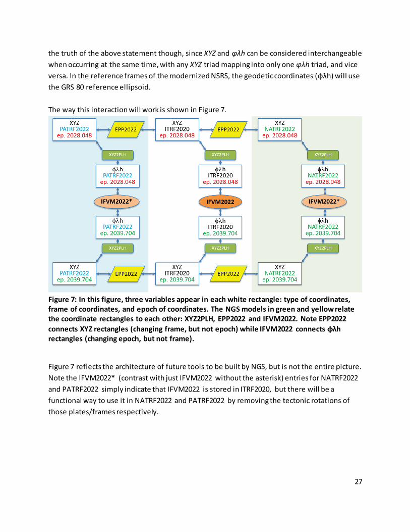
the truth of the above statement though, since XYZ and φλh can be considered interchangeable when occurring at the same time, with any XYZ triad mapping into only one φλh triad, and vice versa. In the reference frames of the modernized NSRS, the geodetic coordinates (φλh) will use the GRS 80 reference ellipsoid. The way this interaction will work is shown in Figure 7.

Figure 7: In this figure, three variables appear in each white rectangle: type of coordinates, frame of coordinates, and epoch of coordinates. The NGS models in green and yellow relate the coordinate rectangles to each other: XYZ2PLH, EPP2022 and IFVM2022. Note EPP2022 connects XYZ rectangles (changing frame, but not epoch) while IFVM2022 connects φλh rectangles (changing epoch, but not frame).

Figure 7 reflects the architecture of future tools to be built by NGS, but is not the entire picture. Note the IFVM2022* (contrast with just IFVM2022 without the asterisk) entries for NATRF2022 and PATRF2022 simply indicate that IFVM2022 is stored in ITRF2020, but there will be a functional way to use it in NATRF2022 and PATRF2022 by removing the tectonic rotations of those plates/frames respectively.

28

10 Updating and Replacing the Four Terrestrial Reference Frames All of the preceding information has dealt with the initial roll-out of NATRF2022, PATRF2022, CATRF2022 and MATRF2022 (and all of their associated components). However, a variety of things will drive updates to these frames, while only certain severe threshold changes to our understanding of the Earth would drive a complete replacement of any of them. Due to the complexity of this situation, the version numbering proposed in this document is tentative.

10.1 Updating the Reference Frames and Their Associated Components The year “2022” occurs in many names listed above. Having that year in all of the various names reflects the fact that these four frames, as well as their defining parameters (EPP2022), their common deformation model (IFVM2022) and their state plane projection parameters (SPCS2022) were originally created for rollout in 2022. The year 2022 does not imply an epoch of the static components of any of the data. Nor does it imply that coordinates in those frames will refer to the year 2022. Nor is 2022 a version number. Rather it is just a convenient way to name the group of things which comprise the modernized NSRS. Because information changes and mistakes are corrected, each frame, as well as the SPCS2022 and the IFVM2022 will occasionally be updated, and each update will come with a respective version number. Some of these version numbers will be related to each other, and others will stand independent. An example of an independent version number is SPCS2022. This set of projections will be released with an initial version number of “1.0.” Updates to any portion of SPCS2022 (adding a layer to a state, changing projection parameters for a state, etc.) will cause a version number change to the entire SPCS2022 set. However, the version number associated with SPCS2022 will stand entirely separate from the version numbers of the frames themselves. As for the frames themselves, even though they are expected to be predominantly applied to areas on or near the tectonic plates for which the frames are named, each is a global frame. Therefore it is difficult to definitely restrict an update to a “local” issue for a single frame. Nonetheless, it is possible that the frames will be updated on different cycles from one another, and therefore NGS will allow for version numbers to differ, from frame to frame.

29

Part of this local/global difficulty can be seen in the case of IFVM2022. This is because there will be one, and only one, deformation model used across all four frames, and that one deformation model has a direct relation to the geodetic coordinates in each of the four frames. This singular nature of IFVM2022 is best exemplified by considering that the movement of any geodetic control point anywhere on Earth can, with perfect equality, be described as any of these five things:

1) Movement in ITRF2020 2) (a) Movement in NATRF2022 plus (b) the rotation of NATRF2022 relative to ITRF2020 3) (a) Movement in PATRF2022 plus (b) the rotation of PATRF2022 relative to ITRF2020 4) (a) Movement in CATRF2022 plus (b) the rotation of CATRF2022 relative to ITRF2020 5) (a) Movement in MATRF2022 plus (b) the rotation of MATRF2022 relative to ITRF2020

For example, if a change in the local crustal deformation modeling in, say, Guam were to occur, that would drive a change to IFVM2022. IFVM2022 might well be applied most frequently in certain regions to certain frames (such as Guam and MATRF2022), but that does not change the nature of IFVM2022 being a single model, used across four global reference frames. In such a case as Guam, which resides wholly on the Mariana plate, it is simple to think in terms of the “Mariana plate deformation portion of IFVM2022”, but that is technically incorrect. IFVM2022 describes intra-frame motions, not intra-plate motions. This is perhaps clearest in southern California. Plate rotations and plate deformations in that region will cause movements of geodetic control points, as in any location. However neither the NATRF2022 nor PATRF2022 frames perfectly describe the rotational movement of the crust in that region and therefore IFVM2022 will contain large residual velocities, whether one considers them relative to NATRF2022 or relative to PATRF2022. If one were to “split” IFVM2022 into, say a North American and Pacific “portion,” then the question must be asked: Which portion would be updated in southern California? This question is a red herring since, as mentioned earlier, IFVM2022 is a single model and describes intra-frame, not intra-plate motions. This means that any update to IFVM2022 should, ostensibly, mean a version number update to the whole model. Further complicating this issue is the desire by NGS and CGS to maintain and work in NATRF2022 collaboratively. As the Canadian government is not particularly interested in the Pacific, Caribbean, or Mariana territories of the USA (nor the frames that support them), it is difficult to flesh out a perfect plan for version numbers that may be driven by updates far from Canada. Therefore, NGS and CGS will form a joint committee on version numbering that will

30

attempt to fully define how this task will be accomplished in a way that is suitable to both governments. Although not optimal, it may come to pass that NGS and CGS maintain separate version numbers of NATRF2022 and maintain a mapping between each agency’s version numbers. These decisions will likely be hashed out over the coming years and by the joint committee. Note that EPP2022 is not discussed above. This is because the relationship between each frame and ITRF2020 is defined through EPP2022. Changing EPP2022 will mean, not an update, but a replacement of a frame (and subsequently a name change), as addressed in the next section. When an update occurs, the definitional epoch of the frames is not changed. That is, the epoch used to relate NATRF2022 (v1.0) to ITRF2020 will be the same as that which relates NATRF2022 (v1.1 or v2.0 or etc.) to ITRF2020 (being 2020.00 in both cases). This updating of the reference frames with version numbers, rather than name changes, is a new policy at NGS. Only an actual replacement of an entire reference frame will trigger a name change. That is, should the first update to NATRF2022 (not a replacement) occur in 2030, NGS will issue “NATRF2022 (v1.1)” and not “NATRF2030.” The capability to access prior versions of NATRF2022 (or other frames) and all its components will be built into NGS products and services. The initial versions of NATRF2022 (or other frames) and all its components will therefore have version “(v1.0)” upon initial rollout.

10.2 Drivers of Updates Updates are either corrections or else significant improvements to the frame. It would be difficult to list all the possible ways an update will occur. Rather, it may be illustrative to consider some of the things that will not drive an update. For example, the creation of a new set of reference epoch coordinates (RECs) at five or ten year intervals will not trigger a new version number, since this will not change the previous set of RECs at an earlier epoch – it will rather just be an expansion of the information within the current version of each frame. Future earthquakes will not necessarily drive an update: this will depend upon location and impact on geodetic control marks. On the other hand, if an earthquake causes a substantive number of CORSs to have incorrect active coordinates (ACs), this would likely trigger a new re-processing of all stations and such a re-processing would yield a new version number. Most of these updates would affect the decimal(s) side of the version (*.1 , *.2, or perhaps *.0.1, *.0.2 etc.). However if a new ITRF is released, and the frames are updated to reflect the

31

new ITRF, then this would also yield an update, but the integer version number will change (1.*, 2.*, etc.) This is more thoroughly discussed in the next section.

10.2.1 New Versions of the ITRF NGS is regularly asked, “What will you do when the next version of the ITRF is released?” The answer is that this will not necessarily cause an update nor a replacement of the terrestrial reference frames. NGS will adopt new orbits and active coordinates at CORSs based on the new ITRF, but the fundamental definition of each frame (being the EPPs within the ITRF2020 frame) will not have changed. Rather, NGS will rely on the official transformations between the new ITRF and ITRF2020, for providing access to the terrestrial reference frames based on the new ITRF. See below.

Figure 8: Accessing the modernized NSRS both before and after a new ITRF is released

So for the initial release of the modernized NSRS, all four frames will have version numbers 1.0. Small, incremental updates, while still working relative to ITRF2020 will yield version numbers 1.1 or perhaps 1.0.1, etc. But when a new ITRF is released, this will trigger versions 2.0 to be computed and released for the four frames.

10.3 Replacing the Terrestrial Reference Frames NGS plans to maintain the terrestrial reference frames under their original names (NATRF2022, etc.) for the foreseeable next few decades. However, as mentioned earlier, the EPPs define the frames. If, in the future, the EPPs are found to be in error, then the definition of a reference frame is no longer valid. The threshold for “in error” has not yet been determined, but will be done so in a coordinated effort between NGS and the Canadian Geodetic Survey.

32

In addition, scientific advances and technological improvements unforeseen in this era could drive a change if scientific and computing techniques of today become superseded in the future.

11 Summary Four new terrestrial reference frames, each mathematically defined so that it rotates in a way to match the motion of a given tectonic plate will be defined relative to ITRF2020. These rotations will be captured in a tool called EPP2022. Any velocities measured at geodetic control points which differ from plate rotation, will be provided as residual intra-frame velocities on those points. These intra-frame velocities will be captured in a tool called IFVM2022. The IFVM2022 tool will be stored in the ITRF2020 and will attempt to model all movements in geodetic latitude, geodetic longitude, and ellipsoidal height of all geodetic control points within the NSRS. When used within one of the plate-fixed frames of the modernized NSRS, IFVM2022 will be modified within NGS tools to remove plate rotation so that it yields residual motions within those plate-fixed frames.

12 Bibliography Goudarzi, M.A.M. Cocard, and R. Santerre, (2014). “EPC: Matlab Software to Estimate Euler Pole Parameters,” GPS Solutions (2014) 18:153–162. https://doi.org/10.1007/s10291-013-0354-4. Altamimi, Z., P. Rebischung, L. Metivier, and X. Collilieux, (2016). “ITRF2014: A new release of the International Terrestrial Reference Frame modeling nonlinear station motions”, Journal of Geophysical Research: Solid Earth 121: 6109-6131. https://doi.org/10.1002/2016JB013098. Bevis, M., A. Brown, and E. Kendrick (2013). “Devising Stable Geometrical Reference Frames for Use in Geodetic Studies of Vertical Crustal Motion,” Journal of Geodesy, 87: 311–321. https://doi.org/10.1007/s00190-012-0600-5. Bevis, M. and A. Brown (2014). “Trajectory Models and Reference Frames for Crustal Motion Geodesy,” Journal of Geodesy, 88: 283–311. https://doi.org/10.1007/s00190-013-0685-5.

33

Blewitt, G., C. Kreemer, and B. Hammond, (2016). “Fixing a Reference Frame to Moving and Deforming Continent,” 2016 AGU Fall Meeting, San Francisco. Dennis, M.L., (2018). The State Plane Coordinate System: History, Policy, and Future Directions. NOAA Special Publication NOS NGS 13. https://www.ngs.noaa.gov/library/pdfs/NOAA_SP_NOS_NGS_0013_v01_2018-03-06.pdf Dixon, T., F. Amelung, A. Ferretti, et al. (2006). “Subsidence and Flooding in New Orleans,” Nature 441, 587–588. https://doi.org/10.1038/441587a. Leick, A. and B.H.W. van Gelder, (1975). “On Similarity Transformations and Geodetic Network Distortions Based on Doppler Satellite Observations,” Reports of the Department of Geodetic Science, No. 235, The Ohio State University, Columbus, Ohio. NGS, (2019). “Blueprint for 2022, Part 3: Working in the Modernized NSRS (first edition),” NOAA Technical Report NOS NGS 67. https://www.ngs.noaa.gov/PUBS_LIB/NOAA_TR_NOS_NGS_0067.pdf NGS, (2021a). “Blueprint for the Modernized NSRS, Part 2: Geopotential Coordinates,” NOAA Technical Report NOS NGS 64. https://www.ngs.noaa.gov/PUBS_LIB/NOAA_TR_NOS_NGS_0064.pdf NGS, (2021b). “Blueprint for the Modernized NSRS, Part 3: Working in the Modernized NSRS (2nd edition).” NOAA Technical Report NOS NGS 67. https://geodesy.noaa.gov/library/pdfs/NOAA_TR_NOS_NGS_0067.pdf Rapp, R., (1989). “Geometric Geodesy, Part II,” Textbook for Advanced Geometric Geodesy, The Ohio State University, Columbus, Ohio. Rebischung, P. and R. Schmid, (2016). “IGS14/igs14.atx: A New Framework for the IGS Products,” 2016 AGU Fall Meeting, San Francisco. Schwarz, Charles R. ed., (1989). North American Datum of 1983. NOAA Professional Paper NOS 2. National Geodetic Survey, Charting and Geodetic Services, National Ocean Service. Rockville, Maryland. https://geodesy.noaa.gov/PUBS_LIB/NADof1983.pdf.

34

Smith, D., (2017). “The Impact of Errors in Euler Pole Parameters on TRF2022 Coordinates,” Presented at the 2017 Fall Meeting of the American Geophysical Union. Available at: https://www.ngs.noaa.gov/web/science_edu/presentations_library/files/2017_12_errors_from_plate_rotation_models_-_agu_-_v02.pptx. Smith, D. and A. Bilich, (2019). “NADCON 5.01,” NOAA Technical Memorandum NOS NGS 81. https://geodesy.noaa.gov/library/pdfs/NOAA_TM_NOS_NGS_0081.pdf. Smith, D., (2020). “Quantifying Systematic Error When Using Axial Rotation Rates Rather Than Geographic Euler Pole Parameters When Describing Tectonic Plate Rotation,” NOAA Technical Memorandum NOS NGS 86. https://geodesy.noaa.gov/library/pdfs/NOAA_TM_NOS_NGS_0086.pdf Soler, T. and J. Marshall, (2003). A Note on Frame Transformations with Applications to Geodetic Datums, available at: https://www.ngs.noaa.gov/CORS/Articles/GPSTrans2.pdf. Stanaway, R., C. Roberts, C. Rizos, N. Donnelly, C. Crook, and J. Haasdyk, (2014). “Converting Plate Rotation Rates about the ITRS Axes to Euler Pole Notation,” REFAG2014 conference, Luxembourg. Wegener, A. (1929), The Origin of Continents and Oceans. Trans. by John Biram (1966). , New York:Dover Publications, Inc.. p. 272.

Appendix A: Euler Pole Parameters

Relationship between an Ideal Frame and a Plate Fixed Frame This appendix will derive the mathematical relationship between XYZ coordinates in the ITRF and the XYZ coordinates in one of the four plate-fixed frames of the modernized NSRS. This derivation is generalized and can be applied to any pair of frames where one is a “global plate-independent frame” (a global frame without any net rotation, such as ITRF2020) and the other is a “plate-fixed frame” (a global frame that attempts to remove the rotation of one tectonic plate, such as NATRF2022, PATRF2022, CATRF2022 or MATRF2022.) Let us begin by presuming that we have a generic global plate-independent frame, which we call RF1, and in which ECEF coordinates of any moving point are time-dependent and

35

designated (X1(t) Y1 (t) Z1(t)). See Figure 8. Earth’s surface is shown in Figure 8 idealized as a sphere.

Figure 9: Global Plate-Independent Coordinate Frame RF1.

Also, assume that some rigid tectonic plate sits on the surface of the Earth, and is rotating about an Euler pole 14. Assume that we know the co-latitude 15 (θ0) and longitude (λ0) of the Euler pole, in RF1, and also the angular velocity of the tectonic plate about that pole, �̇�𝜔0. See Figure 9. However, before proceeding, a subtle, but critical point should be made: The Euler pole’s location in RF1 (co-latitude and longitude of θ0 and λ0) is (for now) presumed to be not moving over time 16.

14 For simplicity, a spherical Earth model will be used in this report. However, the ell ipsoidal nature of the Earth does introduce a 2nd order effect. However, this has been investigated by others, and found to be negligible (see Appendix B of Bevis, Brown, and Kendrick 2013.) 15 Co-latitude, rather than latitude, is used here to simplify latter equations and derivations. 16 Like any modeled quantity, there is uncertainty not only in the Euler pole’s location but possibly in its stability within RF1 itself. Any such uncertainty or instability will be estimated by NGS but will not propagate into the coordinates and uncertainties in the four terrestrial reference frames. This decision is primarily driven by the expected size of uncertainties in the CATRF2022 and MATRF2022 components of EPP2022. This is expected to be published in a forthcoming NOAA technical memorandum.

36

Figure 10: A Rotating Tectonic Plate (Green) and Its Euler pole (Dashed Green Arrow & Red Dot).

We are ultimately going to create a new frame, called RF3, the reason for which will become clear soon. To do so, requires first creating an intermediate frame, RF2. First, let us perform a counter clockwise rotation of RF1 about its Z1 axis by λ0, in order to create RF2 where the Euler pole now lies in the X2-Z2 plane of RF2. See Figure 10.

Figure 11: Creating RF2 by rotating RF1 about the Z1 axis by λ0.

37

The mathematical relationship between coordinates in two Cartesian frames (related through a single rotation) is well known and will be presented momentarily. Because the θ0 and λ0 are assumed to be time-independent, as we write the relationship between coordinates in RF1 and coordinates in RF2, any epoch may be chosen. Therefore (and for reasons that will be clear later) we will explicitly write out two equations; the first for some specific epoch t=t0, and the second for any generic epoch “t.”

�𝑋𝑋2𝑌𝑌2𝑍𝑍2�𝑡𝑡0

= �cos𝜆𝜆0 sin 𝜆𝜆0 0−sin 𝜆𝜆0 cos 𝜆𝜆0 0

0 0 1� �𝑋𝑋1𝑌𝑌1𝑍𝑍1�𝑡𝑡0

= 𝑅𝑅1𝜆𝜆0 �

𝑋𝑋1𝑌𝑌1𝑍𝑍1�𝑡𝑡0

(4)

�𝑋𝑋2𝑌𝑌2𝑍𝑍2�𝑡𝑡

= �cos 𝜆𝜆0 sin 𝜆𝜆0 0−sin 𝜆𝜆0 cos 𝜆𝜆0 0

0 0 1� �𝑋𝑋1𝑌𝑌1𝑍𝑍1�𝑡𝑡

= 𝑅𝑅1𝜆𝜆0 �

𝑋𝑋1𝑌𝑌1𝑍𝑍1�𝑡𝑡

(5)

Note that the R1 matrix is not time dependent, and therefore is the same in these two equations. Now proceeding to the creation of RF3, rotate RF2 counterclockwise about its Y2 axis by θ0 to establish RF3 that has its Z3 axis pointing along the Euler pole axis. See Figure 11.

Figure 12: Creating RF3 by rotating RF2 about the Y2 axis by θ0.

As before (with RF1 and RF2), we can now write the relationship between RF1 coordinates and RF3 coordinates at any epoch, since the Euler pole isn’t moving.

38

�𝑋𝑋3𝑌𝑌3𝑍𝑍3�𝑡𝑡0

= �cos𝜃𝜃0 0 −sin 𝜃𝜃0

0 1 0sin 𝜃𝜃0 0 cos𝜃𝜃0

� �𝑋𝑋2𝑌𝑌2𝑍𝑍2�𝑡𝑡0

= 𝑅𝑅2𝜃𝜃0 �

𝑋𝑋2𝑌𝑌2𝑍𝑍2�𝑡𝑡0

= 𝑅𝑅2𝜃𝜃0𝑅𝑅1

𝜆𝜆0 �𝑋𝑋1𝑌𝑌1𝑍𝑍1�𝑡𝑡0

(6)

�𝑋𝑋3𝑌𝑌3𝑍𝑍3�𝑡𝑡

= �cos𝜃𝜃0 0 − sin 𝜃𝜃0

0 1 0sin 𝜃𝜃0 0 cos 𝜃𝜃0

� �𝑋𝑋2𝑌𝑌2𝑍𝑍2�𝑡𝑡

= 𝑅𝑅2𝜃𝜃0 �

𝑋𝑋2𝑌𝑌2𝑍𝑍2�𝑡𝑡

= 𝑅𝑅2𝜃𝜃0𝑅𝑅1

𝜆𝜆0 �𝑋𝑋1𝑌𝑌1𝑍𝑍1�𝑡𝑡

(7)

As with R1, the R2 matrix is also time-independent. To be explicit: RF1, RF2, and RF3 all have a fixed orientation to one another over time. These frames do not rotate over time. However, a point sitting on a rigid tectonic plate, rotating about the Euler pole will have time-dependent coordinates in all three frames. It just so happens that the computation of that time dependency, as described below, is much simpler in RF3 than in the other two frames, which is why RF3 was introduced. Since RF3 has its Z3 axis aligned with the Euler pole, then the time-dependent RF3 coordinates (X3, Y3, Z3) of a point sitting on a plate that rotates about the Euler pole may very easily be computed simply by applying a rotation of that point about the Z3 axis to those coordinates. This is where the introduction of t0 comes in. The time t0 will represent some reference epoch, from which differences in coordinates over time will be computed. To do so, first, assume the time elapsed since epoch t0 is Δt, where Δt=t-t0. Then, assume the angular velocity of the plate rotation about the Euler pole is �̇�𝜔0 (in, say, milli-arcseconds per year). As with the location of the pole, this angular velocity is also assumed constant. Thus, in the time interval between t0 and t, the plate rotated by an angle “α” about the Euler pole (or, equivalently, about the Z3 axis) where α=0Δt=0(t- t0). In order to visualize this, let us view frame #3 from the perspective that both the Z3 axis points upwards, and also that we can see our continent. Let us then identify some point on that continent. See Figure 12.

39

Figure 13: New perspective of RF3. Dot (black) is any point on the tectonic plate at t0.

Before proceeding, a reminder may be warranted: The only motion (of a point) being represented in this appendix is due to fixed rotation rate (of �̇�𝜔0) about a fixed Euler pole (coordinates in RF1 of θ0 and λ0). No other motions are being discussed. For now let us show the motion of the point on the tectonic plate by plotting its location at t0 and t. See Figure 13.

Figure 14: The simple motion of any point over time on the rotating continent, when seen in RF3. Then, the relationship between (X3, Y3, Z3) at time t and (X3, Y3, Z3) at time t0 is just a rotation of the point in RF3 about the Z3 axis by an angle of α:

�𝑋𝑋3𝑌𝑌3𝑍𝑍3�𝑡𝑡

= �cos𝛼𝛼 − sin𝛼𝛼 0sin𝛼𝛼 cos𝛼𝛼 0

0 0 1� �𝑋𝑋3𝑌𝑌3𝑍𝑍3�𝑡𝑡0

= 𝑅𝑅3𝛼𝛼 �𝑋𝑋3𝑌𝑌3𝑍𝑍3�𝑡𝑡0

(8)

40

Note that frame RF3 is not rotating! That is, do not confuse this rotation of a point within RF3 with the rotations earlier (rotating RF1 to create RF2, rotating RF2 to create RF3). This rotation is the rotation of a point in a fixed frame (RF3) and is not creating a new frame, but is expressly defining the Euler-Pole motion (time-dependence) of a point’s coordinates within RF3. For this reason, the rotation matrix in equation 5 is the inverse of the standard rotation matrix about a Z axis. This represents the difference between:

• rotating a frame about its Z axis, and computing the effect on an unmoving point,

• and keeping the frame unmoving, while rotating a point about the frame’s Z axis.

The former type of change was seen in equations 4 and 5. The latter type of change is seen in equation 8. In equation 8, unlike equations 1 through 4, the epoch on the left hand side (t) is different from the epoch on the right hand side (t0). Now, invoking equation #6 and applying it to equation #8 allows us to express the time-dependent RF3 coordinates in terms of coordinates at t0 in RF2 but more importantly in the initial global, plate-independent frame, RF1:

�𝑋𝑋3𝑌𝑌3𝑍𝑍3�𝑡𝑡

= 𝑅𝑅3𝛼𝛼 �𝑋𝑋3𝑌𝑌3𝑍𝑍3�𝑡𝑡0

= 𝑅𝑅3𝛼𝛼𝑅𝑅2𝜃𝜃0𝑅𝑅1

𝜆𝜆0 �𝑋𝑋1𝑌𝑌1𝑍𝑍1�𝑡𝑡0

(9)

However, repeating equation 7 so it can immediately be compared it to equation 6:

�𝑋𝑋3𝑌𝑌3𝑍𝑍3�𝑡𝑡

= 𝑅𝑅2𝜃𝜃0𝑅𝑅1

𝜆𝜆0 �𝑋𝑋1𝑌𝑌1𝑍𝑍1�𝑡𝑡

(10)

Note that equations 9 and 10 have the same left hand side (time-dependent coordinates in RF3). As such, let us set their right hand sides equal to one another:

𝑅𝑅2𝜃𝜃0𝑅𝑅1

𝜆𝜆0 �𝑋𝑋1𝑌𝑌1𝑍𝑍1�𝑡𝑡

= 𝑅𝑅3𝛼𝛼𝑅𝑅2𝜃𝜃0𝑅𝑅1

𝜆𝜆0 �𝑋𝑋1𝑌𝑌1𝑍𝑍1�𝑡𝑡0

(11)

Re-arranging equation 11 yields:

41

�𝑋𝑋1𝑌𝑌1𝑍𝑍1�𝑡𝑡

= �𝑅𝑅1𝜆𝜆0�

−1�𝑅𝑅2

𝜃𝜃0�−1𝑅𝑅3𝛼𝛼𝑅𝑅2

𝜃𝜃0𝑅𝑅1𝜆𝜆0 �

𝑋𝑋1𝑌𝑌1𝑍𝑍1�𝑡𝑡0

(12)

Equation 12 shows the relationship between RF1 coordinates over time and RF1 coordinates at epoch t0 (note its much more complicated nature than the frame 3 relationship from equation 8). In other words, this is defining the Euler-pole motion (time-dependence) of a point’s coordinates within the global plate-independent frame (RF1). The right hand side, reading from right to left, may be interpreted as “start with RF1 coordinates at t0, rotate the axes through RF2 into RF3, then let coordinates change (within RF3) over time Δt as a result of plate rotation, then rotate the axes back to through RF2 into RF1.” For the sake of brevity, combine the 5-rotation matrices on the right hand side of equation 12 into one matrix called “M”:

𝑀𝑀 = �𝑅𝑅1𝜆𝜆0�

−1�𝑅𝑅2

𝜃𝜃0�−1𝑅𝑅3𝛼𝛼𝑅𝑅2

𝜃𝜃0𝑅𝑅1𝜆𝜆0 (13)

Where M is dependent upon θ0, λ0, and α (or �̇�𝜔0 and ∆t):

�𝑋𝑋1𝑌𝑌1𝑍𝑍1�𝑡𝑡

= 𝑀𝑀 �𝑋𝑋1𝑌𝑌1𝑍𝑍1�𝑡𝑡0

(14)

Turning our attention now to some plate-fixed frame, let us refer to its coordinates with lower case letters (x(t), y(t), z(t)). Earlier, we defined plate-fixed in the modernized NSRS, as each tectonic plate having one plate-fixed terrestrial reference frame, where the Cartesian frame will be rigid, and rotate in a way which matches the NGS-adopted Euler pole rotation for that plate. To express this definition mathematically, the two conditions introduced earlier will now be invoked. The first states, in brief, that “if the only motion which a point is experiencing is rotation (of a rigid plate) about an Euler pole, then in a plate-fixed frame (fixed to that rigid plate), the plate-fixed coordinates do not change over time” (Condition 1 above). Thus:

�𝑥𝑥𝑦𝑦𝑧𝑧�𝑡𝑡

= �𝑥𝑥𝑦𝑦𝑧𝑧�𝑡𝑡0

(15)

Equation 15 is only valid for a point whose entire motion (in the global plate-independent frame RF1) is that of rotation about the Euler pole (i.e. it is true only if the plate is rigid and

42

there is no vertical motion at all). These assumptions are generally not true in the real world, as all points are expected to have some intra-frame motion not fully described by the plate’s rotation (whatever their scale in time or space). Equation 15 shows dependence over time of the plate-fixed coordinates to some chosen set of plate-fixed coordinates at some particular epoch t0, but does not state what the actual plate-fixed coordinates are at that epoch. That brings us to the second plate-fixed condition that states “the plate-fixed coordinates at epoch t0 are equal to the global plate-independent frame coordinates at that same epoch” (Condition 2). Mathematically:

�𝑥𝑥𝑦𝑦𝑧𝑧�𝑡𝑡0

= �𝑋𝑋1𝑌𝑌1𝑍𝑍1�𝑡𝑡0

(16)

Note that equation 16 does not require any assumptions about plate rigidity. It simply sets all coordinates in the plate-fixed frame equal to those in the global plate-independent frame, without any regard for where, on the plate, such a point sits; it gives us an initialized set of plate-fixed coordinates. Equations 14–16 are used to derive the relationship between plate-fixed coordinates over time (which is the desired quantity) and global plate-independent frame coordinates over time (which is usually the quantity first computed when using GNSS). Beginning with equation 14, and then invoking equations 16 and then 15, one can see the following:

�𝑋𝑋1𝑌𝑌1𝑍𝑍1�𝑡𝑡

= 𝑀𝑀�𝑋𝑋1𝑌𝑌1𝑍𝑍1�𝑡𝑡0

= 𝑀𝑀 �𝑥𝑥𝑦𝑦𝑧𝑧�𝑡𝑡0

= 𝑀𝑀 �𝑥𝑥𝑦𝑦𝑧𝑧�𝑡𝑡

(17)

Solving equation 17 for the time-dependent plate-fixed coordinates yields:

�𝑥𝑥𝑦𝑦𝑧𝑧�𝑡𝑡

= 𝑀𝑀−1 �𝑋𝑋1𝑌𝑌1𝑍𝑍1�𝑡𝑡

(18)

Where the M-1 matrix can be written (noting that all component matrices of M are invertible):

𝑀𝑀−1 = �𝑅𝑅1𝜆𝜆0�

−1�𝑅𝑅2

𝜃𝜃0�−1

[𝑅𝑅3𝛼𝛼]−1𝑅𝑅2𝜃𝜃0𝑅𝑅1

𝜆𝜆0 (19)

43

What equation 18 states is that a simple rotation matrix, M-1, can provide the connection between time-dependent global plate-independent frame coordinates (which are usually output by a GNSS software package) and the time-dependent plate-fixed coordinates (which are often desired by geospatial professionals working on that plate). What is not obvious from equation 18 is that (in the absence of intra-frame motions) time-dependent plate-fixed coordinates are constant over time (which, as a reminder, is the desired outcome of adopting a plate-fixed reference frame). The derivation of this fact is presented below before proceeding. Our goal is to show that the left hand side of equation 18 is actually time-independent for any point on the tectonic plate that is rotating about our given Euler pole at the set rate of rotation of that plate with no intra-frame motions. Begin by expanding the right hand side of equation 18, using equation 14:

�𝑥𝑥𝑦𝑦𝑧𝑧�𝑡𝑡

= 𝑀𝑀−1 �𝑋𝑋1𝑌𝑌1𝑍𝑍1�𝑡𝑡

= 𝑀𝑀−1𝑀𝑀�𝑋𝑋1𝑌𝑌1𝑍𝑍1�𝑡𝑡0

= �𝑋𝑋1𝑌𝑌1𝑍𝑍1�𝑡𝑡0

(20)

Thus we can see that without intra-frame motions (assuming a rigid, rotating plate without any vertical signals), the plate-fixed coordinates, expressed as a function of time, do not deviate; they are fixed at their initial values, as set at epoch t0 (see equation 16).

Considering a Simplified M-1 Matrix Equation 18 shows the relationship between the global plate-independent frame (such as the ITRF) and some plate-fixed frame. In its fully expanded form it looks like this:

�𝑥𝑥𝑦𝑦𝑧𝑧�𝑡𝑡

= �cos𝜆𝜆0 sin𝜆𝜆0 0−sin𝜆𝜆0 cos𝜆𝜆0 0

0 0 1�−1

�cos𝜃𝜃0 0 −sin𝜃𝜃0

0 1 0sin𝜃𝜃0 0 cos𝜃𝜃0

�

−1

�cos �̇�𝜔0(𝑡𝑡− 𝑡𝑡0) − sin�̇�𝜔0(𝑡𝑡 −𝑡𝑡0) 0sin�̇�𝜔0(𝑡𝑡 −𝑡𝑡0) cos �̇�𝜔0(𝑡𝑡− 𝑡𝑡0) 0

0 0 1�−1

�cos𝜃𝜃0 0 −sin𝜃𝜃0

0 1 0sin𝜃𝜃0 0 cos𝜃𝜃0

� �cos𝜆𝜆0 sin𝜆𝜆0 0−sin𝜆𝜆0 cos𝜆𝜆0 0

0 0 1��𝑋𝑋1𝑌𝑌1𝑍𝑍1�𝑡𝑡

(21)

One good thing about equation 21 is that it is exact (within the assumption that the plate rotation occurs on a sphere, and not an ellipsoid). One bad thing is that equation 21 is a lot of trigonometry and matrix algebra, including three inverses, simply to convert three coordinates into three other coordinates. It would be helpful if a simpler, but equally accurate, version of equation 21 existed. It so happens that it does. In fact there are a few ways to do things more simply.

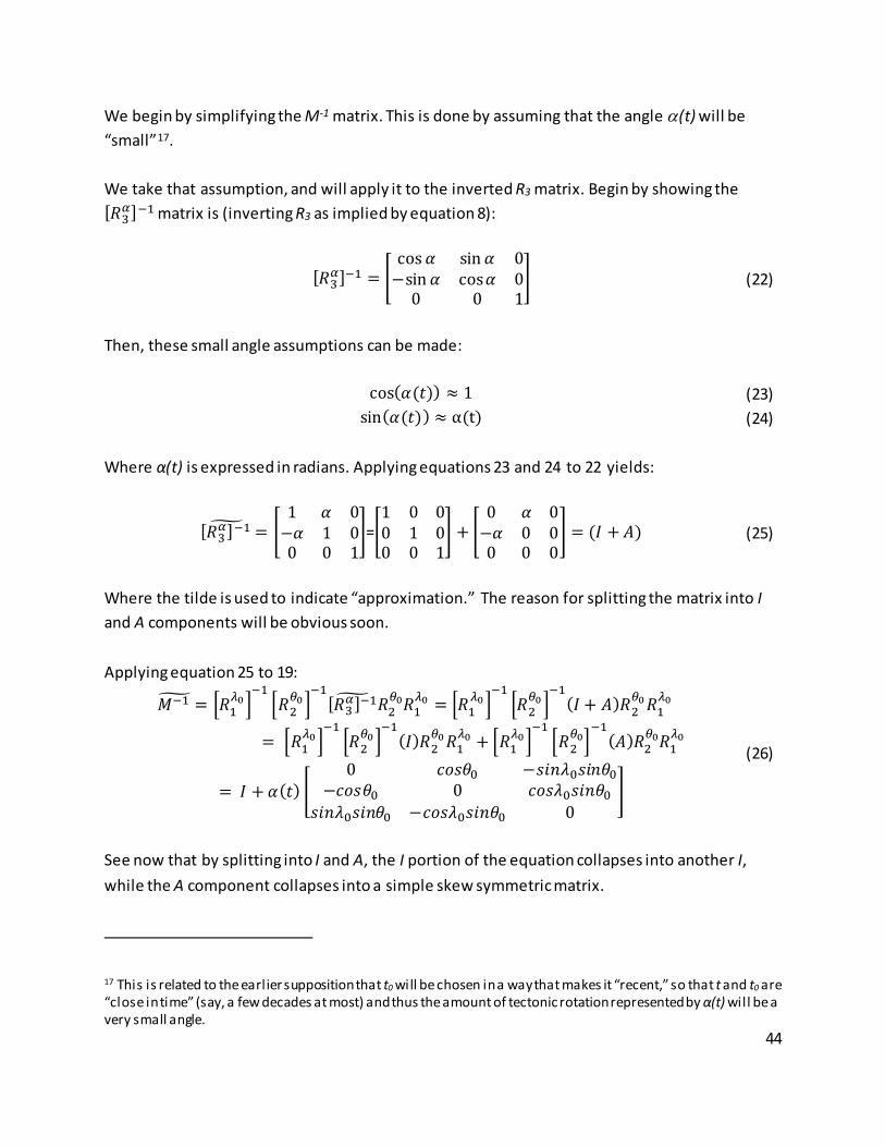
44

We begin by simplifying the M-1 matrix. This is done by assuming that the angle α(t) will be “small”17. We take that assumption, and will apply it to the inverted R3 matrix. Begin by showing the [𝑅𝑅3𝛼𝛼]−1 matrix is (inverting R3 as implied by equation 8):

[𝑅𝑅3𝛼𝛼]−1 = �cos𝛼𝛼 sin𝛼𝛼 0−sin𝛼𝛼 cos𝛼𝛼 0

0 0 1� (22)

Then, these small angle assumptions can be made:

cos(𝛼𝛼(𝑡𝑡)) ≈ 1 (23) sin(𝛼𝛼(𝑡𝑡)) ≈ α(t) (24)

Where α(t) is expressed in radians. Applying equations 23 and 24 to 22 yields:

[𝑅𝑅3𝛼𝛼]−1� = �1 𝛼𝛼 0−𝛼𝛼 1 00 0 1

�=�1 0 00 1 00 0 1

� + �0 𝛼𝛼 0−𝛼𝛼 0 00 0 0

� = (𝐼𝐼 +𝐴𝐴) (25)

Where the tilde is used to indicate “approximation.” The reason for splitting the matrix into I and A components will be obvious soon. Applying equation 25 to 19:

𝑀𝑀−1� = �𝑅𝑅1𝜆𝜆0�

−1�𝑅𝑅2

𝜃𝜃0�−1

[𝑅𝑅3𝛼𝛼]−1� 𝑅𝑅2𝜃𝜃0𝑅𝑅1

𝜆𝜆0 = �𝑅𝑅1𝜆𝜆0�

−1�𝑅𝑅2

𝜃𝜃0�−1

(𝐼𝐼 + 𝐴𝐴)𝑅𝑅2𝜃𝜃0𝑅𝑅1

𝜆𝜆0

= �𝑅𝑅1𝜆𝜆0�

−1�𝑅𝑅2

𝜃𝜃0�−1

(𝐼𝐼)𝑅𝑅2𝜃𝜃0𝑅𝑅1

𝜆𝜆0 + �𝑅𝑅1𝜆𝜆0�

−1�𝑅𝑅2

𝜃𝜃0�−1

(𝐴𝐴)𝑅𝑅2𝜃𝜃0𝑅𝑅1

𝜆𝜆0

= 𝐼𝐼 + 𝛼𝛼(𝑡𝑡) �0 𝑐𝑐𝑐𝑐𝑐𝑐𝜃𝜃0 −𝑐𝑐𝑠𝑠𝑠𝑠𝜆𝜆0𝑐𝑐𝑠𝑠𝑠𝑠𝜃𝜃0

−𝑐𝑐𝑐𝑐𝑐𝑐𝜃𝜃0 0 𝑐𝑐𝑐𝑐𝑐𝑐𝜆𝜆0𝑐𝑐𝑠𝑠𝑠𝑠𝜃𝜃0𝑐𝑐𝑠𝑠𝑠𝑠𝜆𝜆0𝑐𝑐𝑠𝑠𝑠𝑠𝜃𝜃0 −𝑐𝑐𝑐𝑐𝑐𝑐𝜆𝜆0𝑐𝑐𝑠𝑠𝑠𝑠𝜃𝜃0 0

�

(26)

See now that by splitting into I and A, the I portion of the equation collapses into another I, while the A component collapses into a simple skew symmetric matrix. 17 This is related to the earlier supposition that t0 will be chosen in a way that makes it “recent,” so that t and t0 are “close in time” (say, a few decades at most) and thus the amount of tectonic rotation represented by α(t) wil l be a very small angle.

45

The form of M-1 in equation 26 is much simpler than equation 21. In theory, NGS could adopt equation 26 as the definitional relationship between the ITRF and a plate-fixed frame. However things can be even simpler if, instead of working with the standard Euler pole parameters [(co-)latitude and longitude of the Euler pole, and a rotation rate about that pole] NGS were to consider three rotation rates about the ITRF XYZ axes themselves.

Using Three rotation Rates Rather Than (Co-)Latitude, Longitude and Rotation Rate as the Euler Pole Parameters To develop an even simpler form for the definitional relationship between the ITRF and a plate-fixed frame, we borrow from a standard geodetic tool: the 14-parameter Helmert transformation. However, the transformation used below will, of necessity, diverge slightly from the common form of a 14-parameter Helmert transformation due to the treatment of epochs when converting from the ITRF to the four plate-fixed TRFs of 2022. Consider the form of equation 21, which has, on either side of the equals sign, coordinates in two different frames but at the same epoch, “t.” In general terms:

�𝑥𝑥𝑦𝑦𝑧𝑧�𝑡𝑡𝑀𝑀−1 𝑜𝑜𝑜𝑜 𝑀𝑀 𝑑𝑑𝑑𝑑𝑑𝑑𝑑𝑑𝑑𝑑𝑑𝑑𝑑𝑑𝑑𝑑𝑑𝑑 𝑜𝑜𝑑𝑑 𝑑𝑑𝑑𝑑𝑜𝑜𝑑𝑑𝑑𝑑𝑡𝑡𝑑𝑑𝑜𝑜𝑑𝑑�⎯⎯⎯⎯⎯⎯⎯⎯⎯⎯⎯⎯⎯⎯⎯⎯⎯⎯⎯⎯⎯⎯⎯⎯� �

𝑋𝑋1𝑌𝑌1𝑍𝑍1�𝑡𝑡

(27)

Contrast this with the common form of a 14-parameter transformation (Soler and Marshall, 2003; equation 3) that has coordinates, but no velocities, in one frame at a reference epoch “t0” while coordinates and velocities of those same points are in the second frame at some other epoch “t”:

�𝑥𝑥𝑦𝑦𝑧𝑧�𝑡𝑡0

14 𝑃𝑃𝑃𝑃𝑜𝑜𝑃𝑃𝑃𝑃𝑑𝑑𝑡𝑡𝑑𝑑𝑜𝑜 𝑇𝑇𝑜𝑜𝑃𝑃𝑑𝑑𝑇𝑇𝑇𝑇𝑜𝑜𝑜𝑜𝑃𝑃𝑃𝑃𝑡𝑡𝑑𝑑𝑜𝑜𝑑𝑑�⎯⎯⎯⎯⎯⎯⎯⎯⎯⎯⎯⎯⎯⎯⎯⎯⎯⎯⎯⎯⎯⎯�

⎣⎢⎢⎢⎢⎢⎡𝑋𝑋1𝑌𝑌1𝑍𝑍1�̇�𝑋1�̇�𝑌1�̇�𝑍1⎦⎥⎥⎥⎥⎥⎤

𝑡𝑡

(28)

Or:

�𝑥𝑥𝑦𝑦𝑧𝑧�𝑡𝑡0

14 𝑃𝑃𝑃𝑃𝑜𝑜𝑃𝑃𝑃𝑃𝑑𝑑𝑡𝑡𝑑𝑑𝑜𝑜 𝑇𝑇𝑜𝑜𝑃𝑃𝑑𝑑𝑇𝑇𝑇𝑇𝑜𝑜𝑜𝑜𝑃𝑃𝑃𝑃𝑡𝑡𝑑𝑑𝑜𝑜𝑑𝑑�⎯⎯⎯⎯⎯⎯⎯⎯⎯⎯⎯⎯⎯⎯⎯⎯⎯⎯⎯⎯⎯⎯� �

𝑋𝑋1 + (𝑡𝑡 − 𝑡𝑡0)�̇�𝑋1𝑌𝑌1 + (𝑡𝑡 − 𝑡𝑡0)�̇�𝑌1𝑍𝑍1 + (𝑡𝑡 − 𝑡𝑡0)�̇�𝑍1

�

𝑡𝑡

(29)

46

The structure of these two relationships is different, as are their goals. The goal of applying the Euler pole rotation (M-1 matrix) to the global plate-independent in equation 22 (or equation 21) is not to arrive at *TRF2022 coordinates at a reference epoch, but to arrive in that TRF at the same epoch as the ideal frame. Thus a one-to-one correspondence between a standard 14 parameter transformation and equation 21 cannot be drawn. However, with a few modifications, equation 21 can be equated to a modified 14-parameter transformation, and simplified. We take as our guidance the example from Stanaway et al. (2014), who claim that a simple 3-parameter transformation can be developed that will effectively apply the relationship seen in equation 21, where those three parameters are rotation rates about the three axes of the ITRF frame. This is not terribly surprising since there are, in fact, three parameters in equation 21: the two Euler pole coordinates and the rotation rate about that pole. We will derive the form of equation 21 that relies on three rotations next. But to do so requires beginning with the modified 14-parameter transformation, exhibiting a number of presumed zero values and adopting the “small angle approximation,” at which point the derivation becomes much easier. We begin with the general form for a 7-parameter transformation. The Bursa-Wolf version (Rapp, 1989), will be adopted (dropping the subscript “1” from the variables X, Y, and Z for readability):

�𝑥𝑥𝑦𝑦𝑧𝑧� = �

𝑇𝑇𝑥𝑥𝑇𝑇𝑦𝑦𝑇𝑇𝑧𝑧�+ (1 + 𝑐𝑐)𝑅𝑅𝑍𝑍(𝜔𝜔𝑍𝑍)𝑅𝑅𝑌𝑌(𝜔𝜔𝑌𝑌)𝑅𝑅𝑋𝑋(𝜔𝜔𝑋𝑋)�

𝑋𝑋𝑌𝑌𝑍𝑍� (30)

where:

𝑅𝑅𝑋𝑋(𝜔𝜔𝑋𝑋) = �1 0 00 cos𝜔𝜔𝑋𝑋 sin𝜔𝜔𝑋𝑋0 −sin 𝜔𝜔𝑋𝑋 cos𝜔𝜔𝑋𝑋

� (31)

𝑅𝑅𝑌𝑌(𝜔𝜔𝑌𝑌) = �cos𝜔𝜔𝑌𝑌 0 −sin 𝜔𝜔𝑌𝑌

0 1 0sin𝜔𝜔𝑌𝑌 0 cos𝜔𝜔𝑌𝑌

� (32)

𝑅𝑅𝑍𝑍(𝜔𝜔𝑍𝑍) = �cos𝜔𝜔𝑍𝑍 sin𝜔𝜔𝑍𝑍 0−sin𝜔𝜔𝑍𝑍 cos𝜔𝜔𝑍𝑍 0

0 0 1� (33)

47

These rotation matrices are consistent with a positive rotation in the counterclockwise direction of a right-handed coordinate system, when viewed down the axis from the viewpoint of its positive end (Leick and van Gelder, 1975). There are many variations on equation 30: for example with the scale factor (1+s) applied after the transformation vector is applied, or with the scale factor written “(1-s),” or with the rotations positive clockwise, rather than counterclockwise. There is no right or wrong form of these equations, but it is imperative that one clarify which version is being used for which application. In order to create a 14, rather than 7, parameter transformation, one need only make each of the 7 parameters on the right hand side of the above equation time-dependent. However, if both Cartesian triads (left hand side and right hand side) are also made time-dependent this will create our aforementioned modified 14 parameter transformation, of a slightly different nature than that provided in equation 28:

�𝑥𝑥(𝑡𝑡)𝑦𝑦(𝑡𝑡)𝑧𝑧(𝑡𝑡)

� = �𝑇𝑇𝑥𝑥(𝑡𝑡)𝑇𝑇𝑦𝑦(𝑡𝑡)𝑇𝑇𝑧𝑧(𝑡𝑡)

� + (1 + 𝑐𝑐(𝑡𝑡))𝑅𝑅𝑍𝑍(𝜔𝜔𝑍𝑍(𝑡𝑡))𝑅𝑅𝑌𝑌(𝜔𝜔𝑌𝑌(𝑡𝑡))𝑅𝑅𝑋𝑋(𝜔𝜔𝑋𝑋(𝑡𝑡))�𝑋𝑋(𝑡𝑡)𝑌𝑌(𝑡𝑡)𝑍𝑍(𝑡𝑡)

� (34)

where:

⎣⎢⎢⎢⎢⎢⎢⎡𝑇𝑇𝑥𝑥(𝑡𝑡)𝑇𝑇𝑦𝑦(𝑡𝑡)𝑇𝑇𝑧𝑧(𝑡𝑡)𝑐𝑐(𝑡𝑡)𝜔𝜔𝑋𝑋(𝑡𝑡)𝜔𝜔𝑌𝑌(𝑡𝑡)𝜔𝜔𝑍𝑍(𝑡𝑡)⎦

⎥⎥⎥⎥⎥⎥⎤

=

⎣⎢⎢⎢⎢⎢⎢⎡ 𝑇𝑇𝑥𝑥(𝑡𝑡0) + (𝑡𝑡 − 𝑡𝑡0)�̇�𝑇𝑥𝑥𝑇𝑇𝑦𝑦(𝑡𝑡0) + (𝑡𝑡 − 𝑡𝑡0)�̇�𝑇𝑦𝑦𝑇𝑇𝑧𝑧(𝑡𝑡0) + (𝑡𝑡 − 𝑡𝑡0)�̇�𝑇𝑧𝑧𝑐𝑐(𝑡𝑡0) + (𝑡𝑡 − 𝑡𝑡0)�̇�𝑐

𝜔𝜔𝑋𝑋(𝑡𝑡0) + (𝑡𝑡 − 𝑡𝑡0)�̇�𝜔𝑋𝑋𝜔𝜔𝑌𝑌(𝑡𝑡0) + (𝑡𝑡 − 𝑡𝑡0)�̇�𝜔𝑌𝑌𝜔𝜔𝑍𝑍(𝑡𝑡0) + (𝑡𝑡 − 𝑡𝑡0)�̇�𝜔𝑍𝑍⎦

⎥⎥⎥⎥⎥⎥⎤

(35)

For simplicity, we combine the three rotation matrices into one:

𝑅𝑅𝑍𝑍𝑌𝑌𝑋𝑋(𝑡𝑡) = 𝑅𝑅𝑍𝑍(𝜔𝜔𝑍𝑍(𝑡𝑡))𝑅𝑅𝑌𝑌(𝜔𝜔𝑌𝑌(𝑡𝑡))𝑅𝑅𝑋𝑋(𝜔𝜔𝑋𝑋(𝑡𝑡)) (36) Where (dropping the “(t)” time dependency just for readability):

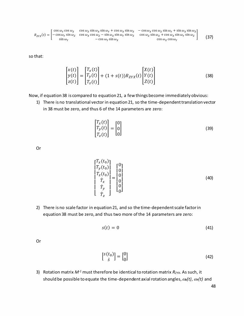
48

𝑅𝑅𝑍𝑍𝑌𝑌𝑋𝑋(𝑡𝑡) = �cos𝜔𝜔𝑌𝑌 cos𝜔𝜔𝑍𝑍 cos𝜔𝜔𝑍𝑍 sin𝜔𝜔𝑋𝑋 sin𝜔𝜔𝑌𝑌 + cos𝜔𝜔𝑋𝑋 sin𝜔𝜔𝑍𝑍 − cos𝜔𝜔𝑋𝑋 cos𝜔𝜔𝑍𝑍 sin𝜔𝜔𝑌𝑌 + sin𝜔𝜔𝑋𝑋 sin𝜔𝜔𝑍𝑍− cos𝜔𝜔𝑌𝑌 sin𝜔𝜔𝑍𝑍 cos𝜔𝜔𝑋𝑋 cos𝜔𝜔𝑍𝑍 − sin𝜔𝜔𝑋𝑋 sin𝜔𝜔𝑌𝑌 sin𝜔𝜔𝑍𝑍 cos𝜔𝜔𝑍𝑍 sin𝜔𝜔𝑋𝑋 + cos𝜔𝜔𝑋𝑋 sin𝜔𝜔𝑌𝑌 sin𝜔𝜔𝑍𝑍

sin𝜔𝜔𝑌𝑌 − cos𝜔𝜔𝑌𝑌 sin𝜔𝜔𝑋𝑋 cos𝜔𝜔𝑋𝑋 cos𝜔𝜔𝑌𝑌

�

(37)

so that:

�𝑥𝑥(𝑡𝑡)𝑦𝑦(𝑡𝑡)𝑧𝑧(𝑡𝑡)

� = �𝑇𝑇𝑥𝑥(𝑡𝑡)𝑇𝑇𝑦𝑦(𝑡𝑡)𝑇𝑇𝑧𝑧(𝑡𝑡)

�+ (1 + 𝑐𝑐(𝑡𝑡))𝑅𝑅𝑍𝑍𝑌𝑌𝑋𝑋(𝑡𝑡)�𝑋𝑋(𝑡𝑡)𝑌𝑌(𝑡𝑡)𝑍𝑍(𝑡𝑡)

� (38)

Now, if equation 38 is compared to equation 21, a few things become immediately obvious:

1) There is no translational vector in equation 21, so the time-dependent translation vector in 38 must be zero, and thus 6 of the 14 parameters are zero:

�𝑇𝑇𝑥𝑥(𝑡𝑡)𝑇𝑇𝑦𝑦(𝑡𝑡)𝑇𝑇𝑧𝑧(𝑡𝑡)

� = �000� (39)

Or

⎣⎢⎢⎢⎢⎢⎡𝑇𝑇𝑥𝑥(𝑡𝑡0)𝑇𝑇𝑦𝑦(𝑡𝑡0)𝑇𝑇𝑧𝑧(𝑡𝑡0)�̇�𝑇𝑥𝑥�̇�𝑇𝑦𝑦�̇�𝑇𝑧𝑧 ⎦

⎥⎥⎥⎥⎥⎤

=

⎣⎢⎢⎢⎢⎡000000⎦⎥⎥⎥⎥⎤

(40)

2) There is no scale factor in equation 21, and so the time-dependent scale factor in

equation 38 must be zero, and thus two more of the 14 parameters are zero:

𝑐𝑐(𝑡𝑡) = 0 (41) Or

�𝑐𝑐(𝑡𝑡0)�̇�𝑐 � = �00� (42)

3) Rotation matrix M-1 must therefore be identical to rotation matrix RZYX. As such, it

should be possible to equate the time-dependent axial rotation angles, ωX(t), ωY(t) and

49

ωZ(t) to the fixed angles of θ0, λ0 and the time-dependent angle α(t) (or its components �̇�𝜔0 ×∆t). That is:

𝑀𝑀−1 = 𝑅𝑅𝑍𝑍𝑌𝑌𝑋𝑋 (43)

Equation 43 is actually an approximation, though the numerical error which arises from adopting it is sub-mm over multiple centuries. Further details can be found in Smith (2020a). Equation 43 tells us that we can adopt the RZYX matrix as the defining matrix between the ITRF and a plate-fixed frame. However this is not terribly helpful yet, as this matrix is complicated (see 21). Thankfully the small angle approximations come into play again:

𝑐𝑐𝑐𝑐𝑐𝑐(𝜔𝜔𝑋𝑋(𝑡𝑡)) ≈ 1 (44) 𝑐𝑐𝑠𝑠𝑠𝑠(𝜔𝜔𝑋𝑋(𝑡𝑡)) ≈ 𝜔𝜔𝑋𝑋(𝑡𝑡) (45) 𝑐𝑐𝑐𝑐𝑐𝑐(𝜔𝜔𝑌𝑌(𝑡𝑡)) ≈ 1 (46)

𝑐𝑐𝑠𝑠𝑠𝑠(𝜔𝜔𝑌𝑌(𝑡𝑡)) ≈ 𝜔𝜔𝑌𝑌(𝑡𝑡) (47) 𝑐𝑐𝑐𝑐𝑐𝑐(𝜔𝜔𝑍𝑍(𝑡𝑡)) ≈ 1 (48)

𝑐𝑐𝑠𝑠𝑠𝑠(𝜔𝜔𝑍𝑍(𝑡𝑡)) ≈ 𝜔𝜔𝑍𝑍(𝑡𝑡) (49) So that matrix RZYX reduces to:

𝑅𝑅𝑍𝑍𝑌𝑌𝑋𝑋� = �1 𝜔𝜔𝑍𝑍(𝑡𝑡) −𝜔𝜔𝑌𝑌(𝑡𝑡)

−𝜔𝜔𝑍𝑍(𝑡𝑡) 1 𝜔𝜔𝑋𝑋(𝑡𝑡)𝜔𝜔𝑌𝑌(𝑡𝑡) −𝜔𝜔𝑋𝑋(𝑡𝑡) 1

� (50)

Which expands (using equation 35) to:

𝑅𝑅𝑍𝑍𝑌𝑌𝑋𝑋�

= �1 𝜔𝜔𝑍𝑍(𝑡𝑡0) + (𝑡𝑡 − 𝑡𝑡0)�̇�𝜔𝑍𝑍 −[𝜔𝜔𝑌𝑌(𝑡𝑡0) + (𝑡𝑡 − 𝑡𝑡0)�̇�𝜔𝑌𝑌]

−[𝜔𝜔𝑍𝑍(𝑡𝑡0) + (𝑡𝑡 − 𝑡𝑡0)�̇�𝜔𝑍𝑍] 1 𝜔𝜔𝑋𝑋(𝑡𝑡0) + (𝑡𝑡 − 𝑡𝑡0)�̇�𝜔𝑋𝑋𝜔𝜔𝑌𝑌(𝑡𝑡0) + (𝑡𝑡 − 𝑡𝑡0)�̇�𝜔𝑌𝑌 −[𝜔𝜔𝑋𝑋(𝑡𝑡0) + (𝑡𝑡 − 𝑡𝑡0)�̇�𝜔𝑋𝑋] 1

� (51)

Although simpler than equation 37, equation 51 can be reduced further. We begin by equating the approximations of M-1 and RZYX to one another (applying equations 51 and 44-49 to equation 43):

50

𝐼𝐼 + 𝛼𝛼(𝑡𝑡) �0 𝑐𝑐𝑐𝑐𝑐𝑐𝜃𝜃0 −𝑐𝑐𝑠𝑠𝑠𝑠𝜆𝜆0𝑐𝑐𝑠𝑠𝑠𝑠𝜃𝜃0

−𝑐𝑐𝑐𝑐𝑐𝑐𝜃𝜃0 0 𝑐𝑐𝑐𝑐𝑐𝑐𝜆𝜆0𝑐𝑐𝑠𝑠𝑠𝑠𝜃𝜃0𝑐𝑐𝑠𝑠𝑠𝑠𝜆𝜆0𝑐𝑐𝑠𝑠𝑠𝑠𝜃𝜃0 −𝑐𝑐𝑐𝑐𝑐𝑐𝜆𝜆0𝑐𝑐𝑠𝑠𝑠𝑠𝜃𝜃0 0

� =

�1 𝜔𝜔𝑍𝑍(𝑡𝑡0) + (𝑡𝑡 − 𝑡𝑡0)�̇�𝜔𝑍𝑍 −[𝜔𝜔𝑌𝑌(𝑡𝑡0) + (𝑡𝑡 − 𝑡𝑡0)�̇�𝜔𝑌𝑌]

−[𝜔𝜔𝑍𝑍(𝑡𝑡0) + (𝑡𝑡 − 𝑡𝑡0)�̇�𝜔𝑍𝑍] 1 𝜔𝜔𝑋𝑋(𝑡𝑡0) + (𝑡𝑡 − 𝑡𝑡0)�̇�𝜔𝑋𝑋𝜔𝜔𝑌𝑌(𝑡𝑡0) + (𝑡𝑡 − 𝑡𝑡0)�̇�𝜔𝑌𝑌 −[𝜔𝜔𝑋𝑋(𝑡𝑡0) + (𝑡𝑡 − 𝑡𝑡0)�̇�𝜔𝑋𝑋] 1

�

(52)

Equation 52 allows for an easy solution to the three axial rotations in terms of the Euler pole’s location and angular velocity:

𝜔𝜔𝑋𝑋(𝑡𝑡0) + (Δ𝑡𝑡)�̇�𝜔𝑋𝑋 = [�̇�𝜔0Δ𝑡𝑡]𝑐𝑐𝑐𝑐𝑐𝑐𝜆𝜆0𝑐𝑐𝑠𝑠𝑠𝑠𝜃𝜃0 (53)

𝜔𝜔𝑌𝑌(𝑡𝑡0) + (Δ𝑡𝑡)�̇�𝜔𝑌𝑌 = [�̇�𝜔0Δ𝑡𝑡]𝑐𝑐𝑠𝑠𝑠𝑠𝜆𝜆0𝑐𝑐𝑠𝑠𝑠𝑠𝜃𝜃0 (54)

𝜔𝜔𝑍𝑍(𝑡𝑡0) + (Δ𝑡𝑡)�̇�𝜔𝑍𝑍 = [�̇�𝜔0Δ𝑡𝑡]𝑐𝑐𝑐𝑐𝑐𝑐𝜃𝜃0 (55) Note: the first term on the left hand side of equations 53, 54, and 55 are all constants, yet there is no corresponding constant value on the right hand side of those equations. For the purposes of convenience, it would be best to invoke Condition #2 from earlier, which means that there should be no difference between the plate-fixed frame and the global plate-independent frame at some chosen reference epoch t0. Thus the constant terms on the left hand side of equations 53–55 should be set to zero. That is:

�𝜔𝜔𝑋𝑋(𝑡𝑡0)𝜔𝜔𝑌𝑌(𝑡𝑡0)𝜔𝜔𝑍𝑍(𝑡𝑡0)

�= �000� (56)

Applying equation 56 to 51 therefore yields the simplest version of the RZYX matrix:

𝑅𝑅𝑍𝑍𝑌𝑌𝑋𝑋� = �1 (𝑡𝑡 − 𝑡𝑡0)�̇�𝜔𝑍𝑍 −(𝑡𝑡 − 𝑡𝑡0)�̇�𝜔𝑌𝑌

−(𝑡𝑡 − 𝑡𝑡0)�̇�𝜔𝑍𝑍 1 (𝑡𝑡 − 𝑡𝑡0)�̇�𝜔𝑋𝑋(𝑡𝑡 − 𝑡𝑡0)�̇�𝜔𝑌𝑌 −(𝑡𝑡 − 𝑡𝑡0)�̇�𝜔𝑋𝑋 1

� (57)

However, for purposes of drawing conclusions later, we will re-write this as:

𝑅𝑅𝑍𝑍𝑌𝑌𝑋𝑋� = 𝐼𝐼 + (𝑡𝑡 − 𝑡𝑡0)�0 �̇�𝜔𝑍𝑍 −�̇�𝜔𝑌𝑌

−�̇�𝜔𝑍𝑍 0 �̇�𝜔𝑋𝑋�̇�𝜔𝑌𝑌 −�̇�𝜔𝑋𝑋 0

� (58)

51

Equation 58 will be the official definitional relationship between ITRF2020 and each of the four plate-fixed reference frames of the modernized NSRS. To use NATRF2022 as an example (replacing 𝑅𝑅𝑍𝑍𝑌𝑌𝑋𝑋� with 𝑅𝑅(𝑡𝑡)𝑁𝑁,𝐼𝐼):

�𝑋𝑋(𝑡𝑡)𝑌𝑌(𝑡𝑡)𝑍𝑍(𝑡𝑡)

�𝑁𝑁

= 𝑅𝑅(𝑡𝑡 , 𝑡𝑡0)𝑁𝑁,𝐼𝐼 �𝑋𝑋(𝑡𝑡)𝑌𝑌(𝑡𝑡)𝑍𝑍(𝑡𝑡)

�𝐼𝐼

(59)

Where “N” means NATRF2022 and “I” means ITRF2020. Expanded out, this reads:

�𝑋𝑋(𝑡𝑡)𝑌𝑌(𝑡𝑡)𝑍𝑍(𝑡𝑡)

�𝑁𝑁

= �𝐼𝐼 + (𝑡𝑡 − 𝑡𝑡0)�0 �̇�𝜔𝑍𝑍 −�̇�𝜔𝑌𝑌

−�̇�𝜔𝑍𝑍 0 �̇�𝜔𝑋𝑋�̇�𝜔𝑌𝑌 −�̇�𝜔𝑋𝑋 0

�𝑁𝑁

��𝑋𝑋(𝑡𝑡)𝑌𝑌(𝑡𝑡)𝑍𝑍(𝑡𝑡)

�𝐼𝐼

(60)

Which can be interpreted as: The X coordinate in NATRF2022 at time “t” can be computed by starting with the X coordinate in ITRF2020 at time “t” and applying the rotations about the Y and Z axes of the ITRF2020 frame over time t-t0. Similarly for the Y and Z coordinates.

Computing the Rotations Assuming that one has solved for (or been given) the standard three Euler pole parameters of (co-)latitude, longitude and rotation rate, it will be interesting and useful to transform those into three rotation rates. After zeroing out the constant terms, equations 53–55 simplify to:

(Δ𝑡𝑡)�̇�𝜔𝑋𝑋 = [�̇�𝜔0Δ𝑡𝑡]𝑐𝑐𝑐𝑐𝑐𝑐𝜆𝜆0𝑐𝑐𝑠𝑠𝑠𝑠𝜃𝜃0 (61) (Δ𝑡𝑡)�̇�𝜔𝑌𝑌 = [�̇�𝜔0Δ𝑡𝑡]𝑐𝑐𝑠𝑠𝑠𝑠𝜆𝜆0𝑐𝑐𝑠𝑠𝑠𝑠𝜃𝜃0 (62)

(Δ𝑡𝑡)�̇�𝜔𝑍𝑍 = [�̇�𝜔0Δ𝑡𝑡]𝑐𝑐𝑐𝑐𝑐𝑐𝜃𝜃0 (63) Dividing by the common term, Δt, on both sides of equations 61–63, the formulae for the rotation rates about the ITRF axes are:

�̇�𝜔𝑋𝑋 = �̇�𝜔0𝑐𝑐𝑐𝑐𝑐𝑐𝜆𝜆0𝑐𝑐𝑠𝑠𝑠𝑠𝜃𝜃0 (64) �̇�𝜔𝑌𝑌 = �̇�𝜔0𝑐𝑐𝑠𝑠𝑠𝑠𝜆𝜆0𝑐𝑐𝑠𝑠𝑠𝑠𝜃𝜃0 (65)

�̇�𝜔𝑍𝑍 = �̇�𝜔0𝑐𝑐𝑐𝑐𝑐𝑐𝜃𝜃0 (66) And just for completeness, inverting equations 64–66 yields the following relationships:

52

𝜃𝜃0 =𝜋𝜋2 − 𝐴𝐴𝐴𝐴𝑐𝑐𝑇𝑇𝐴𝐴𝑠𝑠 �

�̇�𝜔𝑍𝑍

�(�̇�𝜔𝑋𝑋2 + �̇�𝜔𝑌𝑌

2)� (67)

𝜆𝜆0 = 𝐴𝐴𝐴𝐴𝑐𝑐𝑇𝑇𝐴𝐴𝑠𝑠 ��̇�𝜔𝑌𝑌�̇�𝜔𝑋𝑋� (68)

�̇�𝜔0 = ��̇�𝜔𝑋𝑋

2 + �̇�𝜔𝑌𝑌2 + �̇�𝜔𝑍𝑍

2 (69) These relationships are identical (but for the difference in latitude vs co-latitude) to those expressed by Stanaway et al (2014). Similar equations are given in Ali Goudarzi et al, (2014). In summary, while the three common EPPs of (co-)latitude, longitude, and rotation rate can be used to create the M-1 matrix (equation 21), but that matrix is more complex than needed, and a simplified version (accurate for centuries, see Smith, 2020) can instead be adopted using rotations about the ITRF2020 axes. NGS will instead define the official relationship between ITRF2020 and the four NSRS TRFs through equation 59, using the rotation matrix in equation 58.