Embed Size (px)
Citation preview
Nodal Pricing and Transmission Losses: An Application to a Hydroelectric Power System
Jean-Thomas Bernard and Chantal Guertin
June 2002 • Discussion Paper 02-34
Resources for the Future 1616 P Street, NW Washington, D.C. 20036 Telephone: 202–328–5000 Fax: 202–939–3460 Internet: http://www.rff.org
© 2002 Resources for the Future. All rights reserved. No portion of this paper may be reproduced without permission of the authors.
Discussion papers are research materials circulated by their authors for purposes of information and discussion. They have not necessarily undergone formal peer review or editorial treatment.
ii
Nodal Pricing and Transmission Losses: An Application to a Hydroelectric Power System
Jean-Thomas Bernard and Chantal Guertin
Abstract Since January 1, 1997, the wholesale electricity market in the United States has been open to
competition. To satisfy the reciprocity requirements imposed by the Federal Energy Regulatory Commission, Hydro-Québec, a Canadian utility, made its transmission grid accessible to third parties. Under the current regulation, transmission losses are taken into account through a single, constant rate; location and time of use play no role.
Hydro-Québec generates most of its electricity from hydro resources. Long high-voltage power lines link production in the North to consumption centers in the South, where there are interconnections with neighboring areas. We develop an optimization model that allows us to calculate nodal prices on the basis of the opportunity costs of exports. Hydro resources and interconnections with neighbors tend to equalize nodal prices between peak and off-peak periods. However, transmission losses give rise to large price differences between the northern and the southern regions. That the price differences are not taken into account under the current regulation has implications for siting new power stations.
Key Words: Electricity, transmission pricing, hydropower
JEL Classification Numbers: JEL L 94
iii
Contents
Introduction............................................................................................................................. 2
Section 1: A simple model of optimal hydropower use ....................................................... 3
Section 2: A simulation model of Hydro-Québec................................................................. 6
2.1 The deregulation of the U.S. wholesale electricity market........................................... 7
2.2 Hydro-Québec: An overview........................................................................................ 8
2.3 The simulation model ................................................................................................... 8
Section 3: Results .................................................................................................................. 10
Conclusion ............................................................................................................................. 12
References.............................................................................................................................. 20
Notes ....................................................................................................................................... 23
Nodal Pricing and Transmission Losses: An Application to a Hydroelectric Power System
Jean-Thomas Bernard and Chantal Guertin∗
Introduction
The ongoing restructuring of the electric power industry has brought to the fore two topics that had received little attention in public utilities economics: governance and the pricing of electric power transmission services. Until the early 1990s, electricity was provided by vertically integrated monopolies, which were mandated to operate within an assigned area and were subject to government control or regulation. Now that it is possible to generate electricity by small natural gas turbines without incurring significant unit cost increases, economies of scale at the generation stage have changed, but transmission and distribution still have natural monopoly features.1 Technological changes and public pressure to lower electricity prices have undermined the conventional structure of the electric power industry. England was first to privatize the whole industry, in 1990, and introduce competition in electricity generation. Since then, the British model has been adopted with modifications by several countries.2
Competition in electricity generation has led to the deregulation of the wholesale market—that is, the market between producers and local distribution utilities. There are also a few cases of partial or even total retail market deregulation. Reaping the full benefits of competition, however, requires nondiscriminatory access to the transmission grid and proper pricing of transmission services. Following the pathbreaking works of Schweppe et al. (1988) and Hogan (1992), economists have devised optimal transmission pricing rules when the objective is maximization of economic surplus subject to production and transmission capacity constraints while taking into account line losses,
∗ The authors’ affiliations are GREEN, Département d'économique, Université Laval, Sainte-Foy, Québec, Canada, G1K 7P4, and International Institute for Sustainable Development, Winnipeg, Manitoba, Canada, R3B 0Y4, respectively. We would like to thank Professor T. Wildi, Professor M. Roland, and seminar participants of TransÉnergie, Ressources Naturelles Québec, and Resources for the Future for their comments. É. Moyneur provided skillful research assistance. The opinions expressed and any remaining errors are the sole responsibility of the authors.
Resources for the Future Bernard and Guertin
2
loop flows, and reliability criteria. The first-order conditions associated with the maximization of economic benefits under constraints yield the so-called nodal prices, the electricity prices to be paid by users and received by producers at each node to reach the stated objective.3 These prices, which vary from node to node, mostly because of transmission line congestion and losses, can be used to determine the value of transmission rights.4
Thus far, the emphasis has been on weblike transmission networks that link load centers and thermal generating stations and give rise to loop flows.5 For such networks, power producers have some freedom in siting new thermal power plants. Important factors are the load distribution over space, fuel supplies, high-voltage power line corridors, and environmental concerns. Hydropower stations have significantly different features; quite often they are located far from consumption centers and thus require long high-voltage transmission lines. Furthermore, because hydroelectricity is produced by the energy of falling water, whose flow varies over time, imports and exports with adjacent regions play a critical role in balancing supply and demand over the course of the year. If such exchanges take place with neighbors who do not have the same demand patterns, imports must increase during the peak period, and the flow of electricity is reversed in the off-peak period.
Important features of hydro-based electric systems are water use over the annual cycle and losses over the high-voltage power lines. The capacity limits of transmission lines from power sites to consumption centers are not so significant as they are in thermal systems, since transmission line capacities are compatible with upstream power plant capacities. However, the capacity limits of the interconnections with adjacent regions may still be significant.
In this paper, we analyze a simple model of a representative hydroelectric power system, with long transmission lines, limited generation capacity next to large consumption centers, limited availability of water over the annual cycle, and interconnections with adjacent regions. Electricity exports and imports and transmission losses play key roles in determining the opportunity costs at each node. The simple model provides the framework for a seven-node model that is applied to Hydro-Québec, a government-owned utility whose total generating capacity was 36,879 MW (94.4% hydro) at the end of 1996.6 The profit maximization results show that nodal price differences between Montréal, which is the main consumption center, and hydropower
Resources for the Future Bernard and Guertin
3
sites located more than 1,000 kilometers away can be as large as 18%. Under the current regulatory regime, transmission line losses are taken into account by applying a 5.2% flat rate to power injected into the transmission network, irrespective of time or location. This creates an erroneous price signal to developers seeking sites for new power plants.
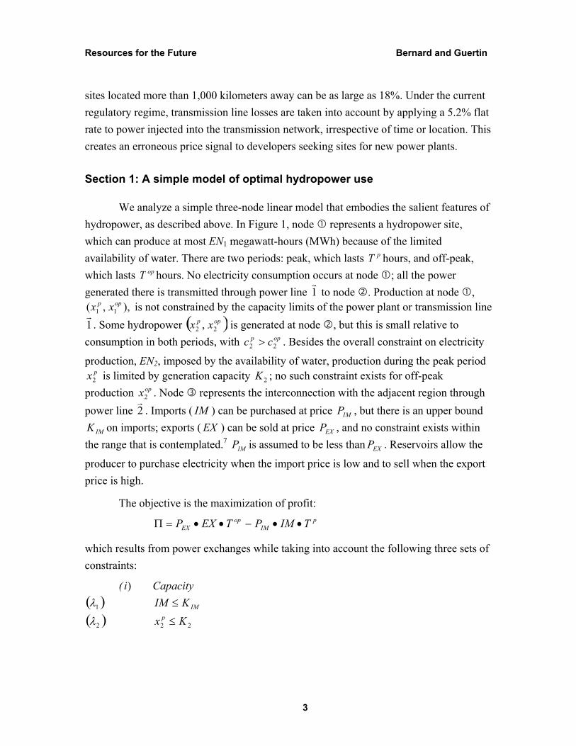
Section 1: A simple model of optimal hydropower use
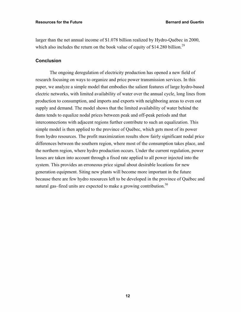
We analyze a simple three-node linear model that embodies the salient features of hydropower, as described above. In Figure 1, node represents a hydropower site, which can produce at most EN1 megawatt-hours (MWh) because of the limited availability of water. There are two periods: peak, which lasts pT hours, and off-peak, which lasts opT hours. No electricity consumption occurs at node ; all the power generated there is transmitted through power line 1
r to node . Production at node ,
),,( 11opp xx is not constrained by the capacity limits of the power plant or transmission line
1r
. Some hydropower ( )opp xx 22 , is generated at node , but this is small relative to consumption in both periods, with opp cc 22 > . Besides the overall constraint on electricity
production, EN2, imposed by the availability of water, production during the peak period px2 is limited by generation capacity 2K ; no such constraint exists for off-peak
production opx2 . Node represents the interconnection with the adjacent region through power line 2
r. Imports ( IM ) can be purchased at price IMP , but there is an upper bound
IMK on imports; exports ( EX ) can be sold at price EXP , and no constraint exists within the range that is contemplated.7 IMP is assumed to be less than EXP . Reservoirs allow the
producer to purchase electricity when the import price is low and to sell when the export price is high.
The objective is the maximization of profit:
pIM
opEX TIMPTEXP ••−••=Π
which results from power exchanges while taking into account the following three sets of constraints:
( )i Capacity ( )1λ IMKIM ≤
( )2λ 22 Kx p ≤
Resources for the Future Bernard and Guertin
4
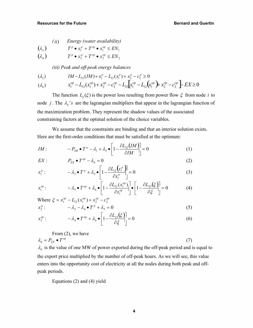
( )ii Energy (water availability) ( )3λ 111 ENxTxT opoppp ≤•+• ( )4λ 222 ENxTxT opoppp ≤•+•
(iii) Peak and off-peak energy balances
)( 5λ 0)()( 22112132 ≥−+−+− pppp cxxLxIMLIM
)( 6λ ( )[ ] 0)( 22112123221121 ≥−−+−−−+− EXcxxLxLcxxLx opopopopopopopop
The function )(ξijL is the power loss resulting from power flow ξ from node i to node j . The sk 'λ are the lagrangian multipliers that appear in the lagrangian function of
the maximization problem. They represent the shadow values of the associated constraining factors at the optimal solution of the choice variables.
We assume that the constraints are binding and that an interior solution exists. Here are the first-order conditions that must be satisfied at the optimum:
IM : ( )
01 3251 =
∂∂
−•+−•−IM
IMLTP p
IM λλ (1)
EX : 06 =−• λopEX TP (2)
px1 : ( )
011
1253 =
∂
∂−•+•− p
plp
xxL
T λλ (3)
opx1 : ( )
01)(1 23
1
11263 =
∂
∂−•
∂
∂−•+•−
ξξ
λλL
xxLT op
opop (4)
Where opopopop cxxLx 221121 )( −+−=ξ px2 : 0542 =+•−− λλλ pT (5)
opx2 : ( )
01 2364 =
∂
∂−•+•−
ξξ
λλL
T op (6)
From (2), we have op
EX TP •=6λ (7)
6λ is the value of one MW of power exported during the off-peak period and is equal to
the export price multiplied by the number of off-peak hours. As we will see, this value enters into the opportunity cost of electricity at all the nodes during both peak and off-peak periods.
Equations (2) and (4) yield
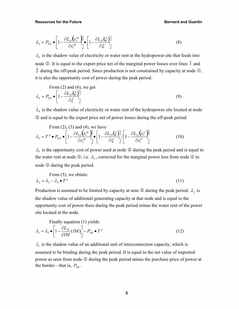
Resources for the Future Bernard and Guertin
5
( ) ( )
∂
∂−•
∂
∂−•=
ξξ
λ 23
1
1123 11
Lx
xLP op
op
EX (8)
3λ is the shadow value of electricity or water rent at the hydropower site that feeds into
node 1. It is equal to the export price net of the marginal power losses over lines 1r
and 2r
during the off-peak period. Since production is not constrained by capacity at node , it is also the opportunity cost of power during the peak period.
From (2) and (6), we get ( )
∂
∂−•=
ξξ
λ 234 1
LPEX (9)
4λ is the shadow value of electricity or water rent of the hydropower site located at node
and is equal to the export price net of power losses during the off-peak period.
From (2), (3) and (4), we have ( ) ( ) ( )
∂
∂−
∂
∂−•
∂
∂−••= p
p
op
op
EXp
xxLL
xxLPT
1
11223
1
1125 1/11
ξξ
λ (10)
5λ is the opportunity cost of power used at node during the peak period and is equal to the water rent at node 1, i.e. 3λ , corrected for the marginal power loss from node 1 to
node 2 during the peak period.
From (5), we obtain: pT•−= 452 λλλ (11)
Production is assumed to be limited by capacity at note 2 during the peak period. 2λ is
the shadow value of additional generating capacity at that node and is equal to the opportunity cost of power there during the peak period minus the water rent of the power site located at the node.
Finally equation (1) yields: p
IM TPIMIML
•−
∂∂
−•= )(1 3251 λλ (12)
1λ is the shadow value of an additional unit of interconnection capacity, which is
assumed to be binding during the peak period. It is equal to the net value of imported power as seen from node 2 during the peak period minus the purchase price of power at the border—that is, IMP .

Resources for the Future Bernard and Guertin
6
In this model, two factors contribute to the equalization of opportunity costs of electricity at each node during the peak and off-peak periods. First is the limited availability of hydropower. As seen from (8) and (9), the water rent associated with hydro production at each node is the same in peak and off-peak periods, and any difference between peak and off-peak opportunity costs at a node reflects the effects of some other constraint, such as generation or transmission capacity; these constraints are binding during the peak period. Second is the power exchange with the neighboring area, which increases supply in the peak period and increases demand in the off-peak period. Furthermore, if the interconnection with the neighbor is close to the main consumption center, as is assumed here, transmission losses tend to decrease in the peak period and increase in the off-peak period. An added benefit of the interconnection is thus the saving on transmission losses.
In the following section we will expand that simple model to build a representation of Hydro-Québec’s electric network in January 1997, when the U.S. wholesale market was opened to competition. The immediate purpose of the expanded applied model is to compute the opportunity costs of power at different nodes during peak and off-peak periods. The theoretical results from the simple three-node model will help us interpret the simulation results in the expanded model.
Section 2: A simulation model of Hydro-Québec
Although the economics literature on optimal nodal pricing is now well developed, only a small number of applications embodying its principles have been implemented so far.8 Very few studies have dealt with the empirical implications of different transmission pricing methods.9
In this paper we focus mainly on transmission losses, limited availability of water, and power exchanges with adjacent areas. We neglect some other elements that have been highlighted in previous studies on transmission pricing—namely, line congestion and loop flows. These two elements of electricity transmission are not so important for hydro-based electric networks when hydropower sites are located far from consumption centers.10
In this section, we first describe the broader context of the wholesale electricity market deregulation that is taking place in the United States and its effects on Canadian
Resources for the Future Bernard and Guertin
7
utilities. This is followed by the presentation of some basic facts about Hydro-Québec. Finally, we show how the available data were used to construct the simulation model.
2.1 The deregulation of the U.S. wholesale electricity market
The wholesale electricity market in the United States has been open to competition since January 1, 1997. Through its Order 888, the Federal Energy Regulatory Commission (FERC) allowed producers, local distribution utilities, and any FERC-licensed marketers to exchange electricity at market prices. This implies that transmission lines must be open to all interested parties in a nondiscriminatory fashion at agreed price schemes.
FERC did not dictate specific pricing schemes for transmission services; rather, it relied upon proposals from interested parties as long as the pricing schemes embodied the general principles of open access to third parties at nondiscriminatory rates. Thus far, three broad methods have been applied to determine transmission rates: flat rate or average cost pricing; zonal rates, which are simply flat rates albeit over small areas; and finally nodal prices, which reflect the marginal costs of producing electricity at various nodes over a network. It should be pointed out that transmission line losses have received little attention from regulatory agencies.
Hydro-Québec applied to FERC for a license to operate as a wholesale marketer in the U.S. market and won approval in late 1997.11 FERC has imposed some reciprocity conditions and requires foreign applicants to open their transmission networks along the lines adopted for the U.S. wholesale market. To satisfy these conditions, Hydro-Québec created a new division, TransÉnergie, which manages all its transmission assets, and the Québec government set the conditions and the rates for open access to the transmission network.12 The government chose one flat rate, which applies to the whole province and does not vary with time of use. The same approach is taken with line losses.
In December 1996, the Québec government created a public utility commission, la Régie de l’énergie, which now has the mandate to approve transmission rates along certain guidelines. Under the proposal of TransÉnergie, a single flat rate of 5.2% would be applied to account for transmission losses; that is, the supplier must provide 1.052 kWh for every kWh to be delivered.
Resources for the Future Bernard and Guertin
8
2.2 Hydro-Québec: An overview13
Hydro-Québec is a government-owned utility that provides electricity to most users in the province of Québec.14 In 1996,15 the vertically integrated utility sold 144.5 TWh to local customers and 19.0 TWh to utilities operating outside the province. Total generation, transmission, and distribution losses were 12.3 TWh. Peak demand reached 31,245 MW in winter because of electric heating; the summer months are part of the off-peak period. The available capacity was 36,679 MW at year’s end, and the hydro share (34,613 MW) was 94.4%.16 One nuclear plant (675 MW) and fuel oil power plants of various sizes (1,391 MW) account for the remaining capacity.
The Hydro-Québec network is interconnected with adjacent regions: Ontario (1,462 MW), New Brunswick (1,050 MW), New York (2,675 MW), and New England (2,300 MW), for a total of 7,487 MW. Because some equipment is used jointly by New York and Ontario, the simultaneous capacity is limited to 6,337 MW.17 Peak demands in New York and New England occur during the summer months. Except for a long-term contract (65 years) to purchase electricity from Labrador, Newfoundland, Hydro-Québec bought little electricity from producers outside the province; the interconnections were used mostly to export power through both long-term contracts (9.6 TWh) and short-term ones (9.4 TWh). On average, Hydro-Québec has been selling more than 10% of its production to its neighbors.
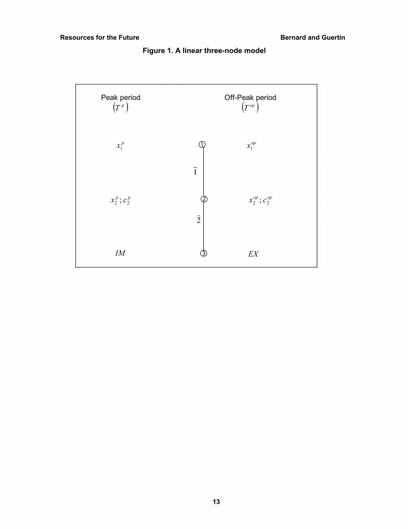
As Figure 2 shows, very large hydro power sites located in the northern part of the province provide the bulk of the hydro capacity: James Bay on the western side with 14,790 MW, and Churchill Falls–Manicouagan-Outardes on the eastern side, with 12,060 MW. Other significant albeit smaller hydro power plants are located in the Trois-Rivières district and on the St. Lawrence River upstream from Montréal. The bulk of the consumption, as well as exports, takes place in the southern part of the province, and high-voltage power lines link production in the North to consumption centers in the South. Some 11,000 kilometers of 735 kV power lines form the backbone of Hydro-Québec’s transmission network. Once power reaches the consumption centers, it is transmitted and distributed at lower voltage.
2.3 The simulation model
The hydro power network shown in Figure 2 is highly complex. To create a simplified model that nevertheless preserves the main characteristics of the network—
Resources for the Future Bernard and Guertin
9
long high-voltage power lines, line losses during peak and off-peak use, variations in the availability of water over the annual cycle, and interconnections with adjacent areas in the southern part of the province—we make several assumptions.18
From administrative districts to nodes
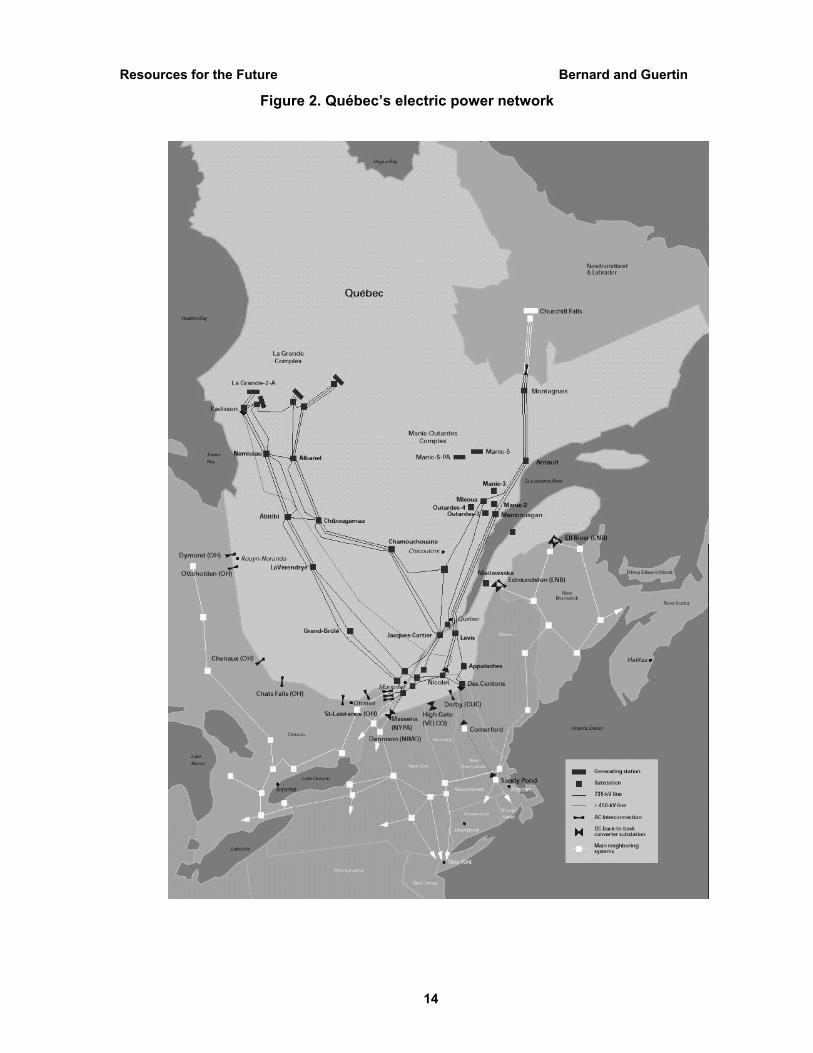
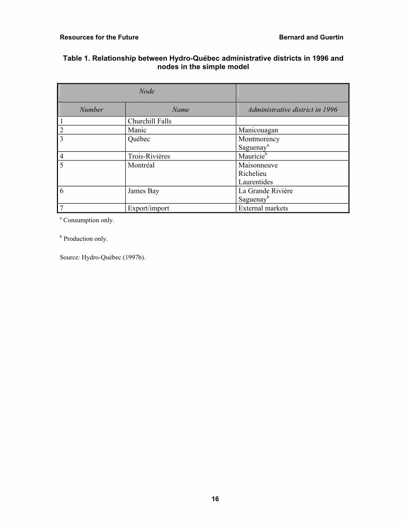
Hydro-Québec high-voltage transmission network is simplified in such a way that each node corresponds to an administrative district (or set of administrative districts) linked by power lines. In this way, the model represents power exchanges between the districts. Table 1 shows the relationships between Hydro-Québec administrative districts in 1996 and the nodes in the simplified model19; Figure 3 illustrates those nodes, the lines, and their length.20
Transmission network and power losses
We assume that there is no congestion over the whole network except at the border, and that all the lines have the same voltage, 735 kV. Power loss (MW) along the line i
r through heat dissipation is determined by the following function:
22)( iii D
VRL ξξ ••=
where
iξ = power input (MW) into line ir
;
R = line resistance per km (Ohms/km); V = voltage (kV);
iD = length of line ir
(km).
Since voltage and line length are given, R has been computed with the calculated power flows between districts during peak and off-peak periods in 1996 and with an average loss factor of 5.2% over total power availability. Our estimate of R is 0.00654.
Demand
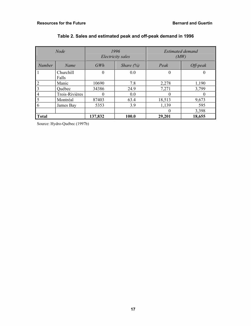
There are two time periods: peak, which lasts 300 hours, and off-peak, which lasts 8,460 hours. Demand is constant within each period. Given the peak demand in 1996, off-peak demand is adjusted so that Hydro-Québec’s annual sales match the sum of peak and off-peak demands. The district (node) shares of consumption within each period are

Resources for the Future Bernard and Guertin
10
the same as the annual shares. Table 2 shows the 1996 actual electricity sales by district21 and the corresponding estimates during peak and off-peak periods. Most of the electricity sales occur in the South: the Montréal district accounts for 63.4%, followed by the Québec district, with 24.9%.
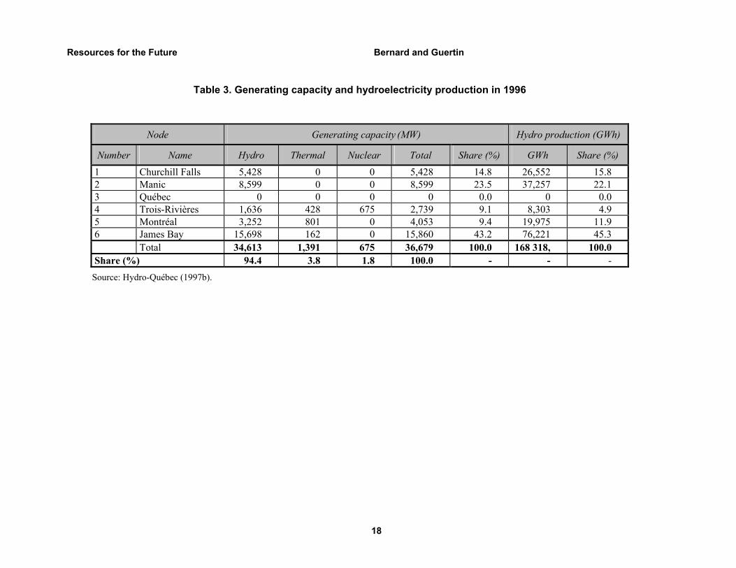
Generating capacity and hydropower output
Table 3 shows the installed generating capacity and hydropower output by district in 1996. Hydropower stations, which accounted for 94.4% of the installed capacity, produced 168,318 GWh in that year. The nuclear station (675 MW) is considered a must-run unit over the whole year.22 Reflecting their current use, the fuel oil power plants are assumed to operate at maximum capacity during the peak period and to be shut down during the off-peak period.
Import and export prices
On the basis of Hydro-Québec’s experience since the opening of the U.S. wholesale electricity market in 1997, the import price is taken to be $40 per MWh, and the export price is set at $50 per MWh.23
Section 3: Results
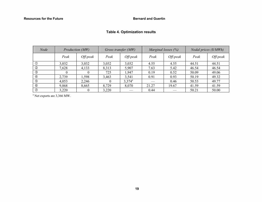
Hydro-Québec’s net profit from export and import is maximized subject to local consumption during peak and off-peak periods while taking into account the available hydroelectricity, generating capacity constraints, nuclear and thermal production, interconnection capacities, and power losses over the transmission lines. The decision variables are imports, exports, and hydropower generation at each node during peak and off-peak periods. The program MAPLE 7 is used to solve the maximization problem; the results appear in Table 4.
Output reaches the maximum capacity level at the Montréal node and at the Trois-Rivières node during the peak period, and imports reach the upper limit of the interconnection capacity at that time. Gross exports are 3,374 MW, less than the maximum. This implies that water used to produce electricity is a scarce resource. Total profit is $1.385 billion. We observe that the relative difference between peak and off-peak production is smaller at nodes located farther from the main consumption centers in the South than at nodes that are nearer. This result comes from the additional supply
Resources for the Future Bernard and Guertin
11
through imports during the peak period and the minimization of power losses over the transmission lines. It turns out that there is no difference between peak and off-peak production for Churchill Falls, which is node . The marginal power losses reveal the joint effects of distance and of power flows; they are small along lines 4,3
rr, and 6
r but
large along lines 2,1rr
, and 5r
.
Table 4 also shows the nodal prices that are set equal to the opportunity costs of power at each node. The export price and the marginal losses are the determining factors. When there are no capacity constraints on production, as at nodes , , and , there are no differences between peak and off-peak nodal prices because hydroelectricity can be moved freely from one period to the other. When production reaches the capacity limit, as at nodes and , however, a price discrepancy between peak and off-peak periods arises, and it shows the shadow value of additional production capacity at these nodes.24 Similarly, the difference between the nodal price of import ($50.21 per MWh) and the price paid to purchase imported power ($40 per MWh) is the shadow value of additional interconnection capacity.
Under the current regulatory regime, a single flat rate of 5.2% applies to all power that is injected into the transmission network to compensate for transmission losses. This means that the net export price is perceived by producers to be $47.53 per MWh. We can see from Table 4 that this price is too low relative to the nodal prices in the southern region, where most of the consumption takes place, and too high in the northern region. This provides an erroneous price signal to developers about where additional plants should be located.25, 26 There is no incentive to build new plants in the southern part of the province, where the opportunity costs are the highest.
If consumption and production of electricity at each node are valued at their respective opportunity costs—that is, at their nodal prices as presented in Table 4—the annual profit is $336 million. This amount falls short of the total revenue requirements of TransÉnergie, which were estimated by Gouvernement du Québec (1997) at $2.260 billion. Some other ways to pay for the capital and operational costs of the transmission network need to be implemented to supplement the income associated with nodal pricing.27
If hydroelectric production at each node is priced at its respective opportunity cost, the gross annual hydroelectric rent is estimated to be $7.372.4 billion, and the rent net of capital and operation costs is estimated to be $2.788.1 billion.28 This amount is
Resources for the Future Bernard and Guertin
12
larger than the net annual income of $1.078 billion realized by Hydro-Québec in 2000, which also includes the return on the book value of equity of $14.280 billion.29
Conclusion
The ongoing deregulation of electricity production has opened a new field of research focusing on ways to organize and price power transmission services. In this paper, we analyze a simple model that embodies the salient features of large hydro-based electric networks, with limited availability of water over the annual cycle, long lines from production to consumption, and imports and exports with neighboring areas to even out supply and demand. The model shows that the limited availability of water behind the dams tends to equalize nodal prices between peak and off-peak periods and that interconnections with adjacent regions further contribute to such an equalization. This simple model is then applied to the province of Québec, which gets most of its power from hydro resources. The profit maximization results show fairly significant nodal price differences between the southern region, where most of the consumption takes place, and the northern region, where hydro production occurs. Under the current regulation, power losses are taken into account through a fixed rate applied to all power injected into the system. This provides an erroneous price signal about desirable locations for new generation equipment. Siting new plants will become more important in the future because there are few hydro resources left to be developed in the province of Québec and natural gas–fired units are expected to make a growing contribution.30
Resources for the Future Bernard and Guertin
13
Figure 1. A linear three-node model
Peak period
( )pT px1
Off-Peak period
( )opT
opx1
pp cx 22 ;
opop cx 22 ;
IM EX
1r
2r
Resources for the Future Bernard and Guertin
14
Figure 2. Québec’s electric power network
Resources for the Future Bernard and Guertin
15
Figure 3. A simplified version of Québec’s electric power network
6 James Bay
5 4 3
7
Montréal
Import/ Export
2
1
Trois-Rivières Québec
Manic
Churchill Falls
node line
( ) line length in km
)1006(5r
)619(1r
)379(2r
)110(3r
)108(4r
)56(6r
Resources for the Future Bernard and Guertin
16
Table 1. Relationship between Hydro-Québec administrative districts in 1996 and nodes in the simple model
Node
Number Name Administrative district in 1996 1 Churchill Falls 2 Manic Manicouagan 3 Québec Montmorency
Saguenaya 4 Trois-Rivières Mauricieb 5 Montréal Maisonneuve
Richelieu Laurentides
6 James Bay La Grande Rivière Saguenayb
7 Export/import External markets a Consumption only.
b Production only.
Source: Hydro-Québec (1997b).
Resources for the Future Bernard and Guertin
17
Table 2. Sales and estimated peak and off-peak demand in 1996
Node 1996 Electricity sales
Estimated demand (MW)
Number Name GWh Share (%) Peak Off-peak 1 Churchill
Falls 0 0.0 0 0
2 Manic 10690 7.8 2,278 1,190 3 Québec 34386 24.9 7,271 3,799 4 Trois-Rivières 0 0.0 0 0 5 Montréal 87403 63.4 18,513 9,673 6 James Bay 5353 3.9 1,139 595 0 3,398 Total 137,832 100.0 29,201 18,655 Source: Hydro-Québec (1997b)
Resources for the Future Bernard and Guertin
18
Table 3. Generating capacity and hydroelectricity production in 1996
Node Generating capacity (MW) Hydro production (GWh)
Number Name Hydro Thermal Nuclear Total Share (%) GWh Share (%)
1 Churchill Falls 5,428 0 0 5,428 14.8 26,552 15.8 2 Manic 8,599 0 0 8,599 23.5 37,257 22.1 3 Québec 0 0 0 0 0.0 0 0.0 4 Trois-Rivières 1,636 428 675 2,739 9.1 8,303 4.9 5 Montréal 3,252 801 0 4,053 9.4 19,975 11.9 6 James Bay 15,698 162 0 15,860 43.2 76,221 45.3 Total 34,613 1,391 675 36,679 100.0 168 318, 100.0 Share (%) 94.4 3.8 1.8 100.0 - - -
Source: Hydro-Québec (1997b).
Resources for the Future Bernard and Guertin
19
Table 4. Optimization results
Node Production (MW) Gross transfer (MW) Marginal losses (%) Nodal prices ($/MWh)
Peak Off-peak Peak Off-peak Peak Off-peak Peak Off-peak
3,032 3,032 3,032 3,032 4.55 4.55 44.51 44.51 7,628 4,133 8,313 5,907 7.63 5.42 46.54 46.54 0 0 725 1,947 0.19 0.52 50.09 49.06 2,739 1,598 3,463 3,541 0.91 0.93 50.19 49.32 4,053 2,246 0 3,374a — 0.46 50.53 49.77 9,868 8,665 8,729 8,070 21.27 19.67 41.59 41.59 3,220 0 3,220 — 0.44 — 50.21 50.00
a Net exports are 3,366 MW.

Resources for the Future Bernard and Guertin
20
References
Bernard, J.-T., and J. Chatel. 1985. The application of marginal cost pricing principles to a hydroelectric system: The case of Hydro-Québec. Resources and Energy 7(4), December: 353–75.
Bernard, J.-T., and J.A. Doucet. 1999. L'ouverture du marché d'exportation d'électricité québécoise: Réalité ou mirage à l'horizon? Canadian Public Policy/Analyse de Politiques XXV(2), June: 247–58.
Bernard, J.-T., and M. Roland. 1997. Rent dissipation through electricity prices of publicly-owned utilities. Canadian Journal of Economics 30(4b), November: 1204–19.
Gilbert, R., and E.P. Kahn (eds.). 1996. International comparisons of electricity regulation. New York: Cambridge University Press.
Gouvernement du Québec. 1997. Conditions et tarifs des services de transport pour l'accessibilité à son réseau. Décret 276-97, Loi sur Hydro-Québec, L.R.Q., c. H-5, 5. Québec, Éditeur officiel du Québec, mars.
Green, R. 1998. Electricity transmission pricing: How much does it cost to get it wrong? Cambridge University, Department of Applied Economics, April.
Guertin, C. 2000. Prix spots et tarification du transport d'électricité: Une application au Québec. M.A. thesis, Université Laval.
Hogan, W.W. 1992. Contract networks for electric power transmission. Journal of Regulatory Economics 4(3), November: 211–42.
Hsu, M. 1997. An introduction to the pricing of electric power transmission. Utilities Policy 63, September: 257–70.
Hydro-Québec. 1997a. Rapport annuel 1996.
Hydro-Québec. 1997b. Historique financier et statistiques diverses 1992–1996. Montréal, Direction principale, Contrôle et comptabilité.
Hydro-Québec. 2001a. Rapport annuel 2000.
Hydro-Québec. 2001b. Plan stratégique 2002–2006.
Resources for the Future Bernard and Guertin
21
Joskow, P., and R.S. Schmalensee. 1983. Markets for power: An analysis of electric utility regulation. Cambridge, MA: MIT Press.
Journal of Regulatory Economics. 1996. Symposium on transmission access 10(1), July.
Schweppe, F.C., et al. 1988. Spot pricing of electricity. New York: Kluwer Academic Publishers.
Utilities Policy. 1997. Special issue on transmission pricing, 6(3), September.


Resources for the Future Bernard and Guertin
23
Notes
1 For an early investigation of the empirical evidence on the extent of economies of scale in electricity generation, see Joskow and Schmalensee (1983). 2 Although there were earlier experiments in, for example, Chile, the British policy change is considered the start of the new era of electricity market deregulation. See papers in Gilbert and Kahn (1996). 3 A node is a consumption center, a producer or set of producers, or a set of high voltage power lines that meet at one point. 4 Hsu (1997) presents a survey of the literature on transmission pricing. See also papers in the Journal of Regulatory Economics (1996) and Utilities Policy (1997). 5 The three-node triangular network provides the standard illustration. 6 More information on Hydro-Québec will be provided in section 2. 7 Import and export capacity limits do not have to be equal, since they depend on the state of the two neighboring electrical systems. If exports reached the capacity limit, this would imply that hydropower was a substitute for imports. Then the import price would determine the opportunity cost of hydroelectricity. 8 Exceptions are New Zealand and the Pennsylvania–New-Jersey–Maryland (PJM) area in the United States. More recently, New York and New England power pools have adopted regulatory regimes for the pricing of transmission services that encompass elements of optimal nodal pricing. 9 One exception is Green (1998), who applies the optimizing approach to the England and Wales electricity system while taking into account transmission capacity constraints and line losses under four pricing regimes of transmission services: nodal pricing, which is taken as the first best case; one uniform price for consumers and nodal prices for producers; nodal prices for consumers and one uniform price for producers; and finally, uniform prices for both consumers and producers. Congestion and transmission line losses are the major factors that lead to price differences between the northern area, which is a net supplier, and the southern area, where the bulk of the demand occurs. 10 Besides Hydro-Québec, British Columbia Hydro and Manitoba Hydro are two other Canadian utilities with transmission networks linking hydropower sites located far from consumption centers. 11 Until then, Hydro-Québec was selling electricity at border points. 12 Gouvernement du Québec (1997). 13 The information presented in this section comes from Hydro-Québec (1997a, 1997b). 14 There are nine municipal distribution utilities that purchase electricity from the Hydro-Québec; they service less than 4% of demand. Private producers, Alcan being the largest, generate another 2,864 MW (96% hydro), mostly for their own use. 15 The most recent year for which district consumption and production data are available is 1996. 16 This includes the 5,428 MW hydro power plant located at Churchill Falls in Labrador, Newfoundland. Through a long-term contract, Hydro-Québec gets nearly all the output from this plant. 17 According to information provided by TransÉnergie, the effective export capacity is approximately 5,500 MW, and the effective import capacity is approximately 3,220 MW. 18 Detailed information on the computation of consumption and production at each node appears in Guertin (2000).

Resources for the Future Bernard and Guertin
24
19 The Matapedia district is omitted because it includes the Gaspé Peninsula and a set of small, isolated networks outside the area served by the main network. It represents less than 0.5% of generation capacity and 4% of annual sales. 20 The approximate distances in kilometers between substations have been provided by TransÉnergie: line1
r,
Churchill-Manicouagan (619 km); line 2r
, Manicouagan–Lévis (379 km); line 3r
Lévis–Nicolet (110 km); line 4r
, Nicolet–Boucherville (Montréal) (108 km); line 5
r, LG2–Chénier (Montréal) (1,006 km); line 6
r, Châteauguay
(Montréal)–Massena (New York) (56 km). 21 There are no electricity sales in the Trois-Rivières district because in 1996 they were recorded in the Montréal and the Québec districts. 22 Its load factor was 94.4% in 1996. 23 All figures are in Canadian dollars. 24 Although no production takes place at node , prices also differ between the peak and off-peak periods through a ripple effect from the constrained nodes. 25 Bernard and Doucet (1999) argued that the average cost pricing of transmission services can lead to misleading price signals for large hydro-based power networks that have long high-voltage transmission lines between generation sites and consumption centers. However, they presented no information on the empirical significance of this effect. 26 The pricing of transmission losses is only one component of the prices associated with transmission services. Under the current regulation regime, average cost pricing is applied to take into account capital and operation costs. Again, location and time of use play no role. 27 Green (1998) arrives at the same conclusion. 28 With 8% as discount rate, the present value is $34.851 billion. 29 This rent is dissipated through low electricity rates to Hydro-Québec local customers. Bernard and Chatel (1985) measured the welfare losses associated with the method of dissipating rents, and Bernard and Roland (1997) explain how electricity provided by a government-owned enterprise, as is the case here, can result in social equilibrium. 30 Hydro-Québec (2001b).