NOISE BENEFITS IN JOINT DETECTION AND ESTIMATION SYSTEMS · NOISE BENEFITS IN JOINT DETECTION AND ESTIMATION SYSTEMS ... NOISE BENEFITS IN JOINT DETECTION AND ... 2.1 Joint detection

NOISE BENEFITS IN JOINT DETECTIONAND ESTIMATION SYSTEMS

a thesis

submitted to the department of electrical and

electronics engineering

and the graduate school of engineering and science

of bilkent university

in partial fulfillment of the requirements

for the degree of

master of science

By

Abdullah Basar Akbay

August, 2014

I certify that I have read this thesis and that in my opinion it is fully adequate,

in scope and in quality, as a thesis for the degree of Master of Science.

Assoc. Prof. Dr. Sinan Gezici (Advisor)



Prof. Dr. Tolga Mete Duman



Asst. Prof. Dr. Mehmet Burak Guldogan

Approved for the Graduate School of Engineering and Science:

Prof. Dr. Levent OnuralDirector of the Graduate School

ii

ABSTRACT

NOISE BENEFITS IN JOINT DETECTION ANDESTIMATION SYSTEMS


M.S. in Electrical and Electronics Engineering

Supervisor: Assoc. Prof. Dr. Sinan Gezici

August, 2014

Adding noise to inputs of some suboptimal detectors or estimators can improve

their performance under certain conditions. In the literature, noise benefits have

been studied for detection and estimation systems separately. In this thesis,

noise benefits are investigated for joint detection and estimation systems. The

analysis is performed under the Neyman-Pearson (NP) and Bayesian detection

frameworks and the Bayesian estimation framework. The maximization of the

system performance is formulated as an optimization problem. The optimal ad-

ditive noise is shown to have a specific form, which is derived under both NP and

Bayesian detection frameworks. In addition, the proposed optimization problem

is approximated as a linear programming (LP) problem, and conditions under

which the performance of the system cannot be improved via additive noise are

obtained. With an illustrative numerical example, performance comparison be-

tween the noise enhanced system and the original system is presented to support

the theoretical analysis.

Keywords: Detection, estimation, linear programming, noise benefits, joint de-

tection and estimation, stochastic resonance.

iii

OZET

BIRLIKTE SEZIM VE KESTIRIM SISTEMLERINDEGURULTUNUN FAYDALARI


Elektrik Elektronik Muhendisligi, Yuksek Lisans

Tez Yoneticisi: Doc. Dr. Sinan Gezici

Agustos, 2014

Belirli kosullar altında, optimal olmayan bazı sezici ve kestiricilerin performansını

girdilerine gurultu ekleyerek gelistirmek mumkundur. Literaturde, gurultunun

faydaları sezici ve kestirici sistemleri icin ayrı ayrı ele alınmıstır. Bu tezde,

birlikte sezim ve kestirim sistemleri icin gurultunun faydaları incelenmektedir.

Analiz, Neyman-Pearson (NP) ve Bayes sezim cerceveleri ve Bayes kestirim

cercevesi altında gerceklestirilmektedir. Sistem performansının en yuksek seviy-

eye cıkarılması, bir optimizasyon problemi olarak tanımlanmaktadır. Optimal

gurultu dagılımının belirli bir istatiksel sekle sahip oldugu gosterilmekte ve bu

optimal gurultu dagılım sekli NP ve Bayes sezim cerceveleri icin ayrı ayrı elde

edilmektedir. Ayrıca onerilen optimizasyon probleminin, bir dogrusal program-

lama (DP) problemi olarak yaklasımı sunulmakta ve sistem performansının DP

yaklasımı altında gurultu ile gelistirilemeyecegi kosullar elde edilmektedir. Bir

sayısal ornek uzerinde, kuramsal bulguları desteklemek amacıyla, gurultu ek-

lenmis sistem ile orijinal sistemin performansları karsılastırılmaktadır.

Anahtar sozcukler : Sezim, kestirim, dogrusal programlama, gurultunun faydaları,

birlikte sezim ve kestirim, stokastik rezonans.

iv

Acknowledgement

I would like to thank my supervisor Assoc. Prof. Dr. Sinan Gezici and express my

gratitude for his valuable guidance, suggestions and encouragement throughout

this work. He is a dignified, kind and considerate academician who is always

benevolent and thoughtful to his students. It is a precious privilege to work with

him. I would like to extend my special thanks to Prof. Dr. Tolga Mete Duman

and Asst. Prof. Dr. Mehmet Burak Guldogan for agreeing to join my thesis

committee with their valuable comments and suggestions on the thesis.

When I first set foot in this institution which instils the passion for learning

into its students, I was just a kid. I do owe every academic success I achieved

and hope to achieve to Bilkent University. I wish to thank Prof. Arıkan, Kozat,

Aktas, Akar and to all the faculty members, and the staff in the Department of

Electrical and Electronics Engineering at Bilkent University.

I wish to thank all my friends who I shared my youth with. It is not possible

to word my feelings, all I can do is expressing my gratitude for being marvellous.

I also extend my special thanks to Mehmet, Oguzhan, Mert, Volkan, Semih, Berk,

Enes, Mohammad, Serkan, Saeed, San and Ahmet for all the amazing memories

of the last two years at Bilkent University.

I also appreciate the value of the financial support from the Scientific and

Technical Research Council of Turkey (TUBITAK).

Finally, my deepest gratitude goes to my parents, my sister Pınar and the rest

of my family for their unconditional love, endless encouragement and continuous

support in every step of my life.

v

Contents

1 Introduction 1

1.1 Objectives and Contributions of the Thesis . . . . . . . . . . . . . 1

1.2 Organization of the Thesis . . . . . . . . . . . . . . . . . . . . . . 5

2 Background and Problem Definition 7

2.1 Background . . . . . . . . . . . . . . . . . . . . . . . . . . . . . . 7

2.1.1 Neyman-Pearson (NP) Hypothesis-Testing Framework . . 9

2.1.2 Bayesian Hypothesis Testing Framework . . . . . . . . . . 11

2.2 Problem Definition . . . . . . . . . . . . . . . . . . . . . . . . . . 12

2.2.1 NP Hypothesis-Testing Framework . . . . . . . . . . . . . 14

2.2.2 Bayesian Hypothesis-Testing Framework . . . . . . . . . . 15

3 Optimal Noise Distribution and Non-Improvability Conditions 17

3.1 Optimum Noise Distribution . . . . . . . . . . . . . . . . . . . . . 17

3.2 Linear Programming Approximation . . . . . . . . . . . . . . . . 20

3.3 Improvability and Non-improvability Conditions . . . . . . . . . . 22

vi

CONTENTS vii

4 Numerical Examples 26

4.1 Analysis of a Given Joint Detection Estimation System . . . . . . 26

4.1.1 Scalar Case, K = 1 . . . . . . . . . . . . . . . . . . . . . . 28

4.1.2 Vector Case, K > 1 . . . . . . . . . . . . . . . . . . . . . . 29

4.1.3 Asymptotic Behaviour of the System, Large K Values . . . 30

4.2 Numerical Results for the Joint Detection and Estimation System 30

5 Conclusion 42

A Derivation of Conditional Estimation Risks 52

B Derivation of Auxiliary Functions 54

C Derivation for Distribution of εK 56

List of Figures

2.1 Joint detection and estimation scheme: Observation signal X is

input to both the detector φ(X) and to the estimator θ(X). An

estimation is provided if the decision is H1. . . . . . . . . . . . . . 9

2.2 Joint detection and estimation scheme with noise enhancement:

The only modification on the original system depicted in Figure 2.1

is the introduction of the additive noise N . . . . . . . . . . . . . . 13

4.1 Noise enhancement effects for the minimization of the conditional

estimation risk, K = 1 (NP framework). . . . . . . . . . . . . . . 33


estimation risk, K = 4 (NP framework). . . . . . . . . . . . . . . 33

4.3 Probability density functions of εk and εK . . . . . . . . . . . . . . 34

4.4 Optimal solutions of the NP problem (3.4) and the solutions of the

linear fractional programming problem defined in (3.6) for K = 1

and σ = 0.3. . . . . . . . . . . . . . . . . . . . . . . . . . . . . . . 35



and σ = 0.3. . . . . . . . . . . . . . . . . . . . . . . . . . . . . . . 35

viii

LIST OF FIGURES ix



and σ = 0.4. . . . . . . . . . . . . . . . . . . . . . . . . . . . . . . 36

4.7 Noise enhancement effects for the minimization of the Bayes esti-

mation risk, K = 1 (Bayes detection framework). . . . . . . . . . 37



4.9 Optimal solutions of Bayes Detection Problem (3.5) and the solu-

tions of the linear programming problem defined in (3.9). K = 1.

σ = 0.5 . . . . . . . . . . . . . . . . . . . . . . . . . . . . . . . . . 38



σ = 0.5 . . . . . . . . . . . . . . . . . . . . . . . . . . . . . . . . . 38



σ = 0.75 . . . . . . . . . . . . . . . . . . . . . . . . . . . . . . . . 39


estimation risk, K = 1 (NP detection framework). . . . . . . . . . 41



List of Tables

4.1 Optimal solutions for the NP based problem (3.4) and the solutions

of the linear fractional programming problem defined in (3.6). . . 34

4.2 Optimal solutions of Bayes detection framework problem (3.5) and

the solutions of the linear programming problem defined in (3.9). 39

x

Chapter 1

Introduction

1.1 Objectives and Contributions of the Thesis

Although an increase in the noise power is generally associated with a perfor-

mance degradation, addition of noise to a system may introduce performance

improvements under certain arrangements and conditions in a number of electri-

cal engineering applications including neural signal processing, biomedical signal

processing, lasers, nano-electronics, digital audio and image processing, analog-

to-digital converters, control theory, statistical signal processing, and information

theory, as exemplified in [1] and references therein. In addition to the electrical

engineering applications, in a broader sense, the observation of benefits of in-

creasing the noise level for enhancing a given system is reported in a variety of

sciences including biology, climatology, chemistry, network science, mathematics,

ecology, finance, and physics [2] (and references therein).

In the literature, this phenomenon is also referred to as “stochastic resonance”

(SR) in some contexts. The term SR was firstly used in [3] within the context

of stochastically behaving dynamical systems. A detailed and concrete analysis

of the response of bistable systems subject to a weak periodic or random signal

is presented in [4]. In order to clarify the SR concept, it is valuable to present a

famous technique “dithering” which is defined as adding a random signal (which

1

can be regarded as noise) to the analog input signal prior to the quantization

operation [5]. In this particular application in digital signal processing, dithered

quantization systems demonstrate SR behaviors and perform superior (reduction

in the averaged quantization error and improvement in the dynamic range) in

comparison to the quantization systems without dithering [6, 7]. Dithering is a

commonly employed technique in audio and image processing, and stands as a

real life application example of noise-enhanced signal processing.

Noise-enhanced signal processing focuses on revealing and analyzing possible

practical benefits of SR phenomenon in the field of signal processing. SR is

initially observed in nonlinear bistable systems driven by a periodic input signal

in the presence of the noise in the form of maximizing the signal to noise ratio

[3, 4, 8, 9]. Later these results are extended into the analysis of the response to

arbitrary aperiodic input signals [10–15]. In addition to these single threshold

SR studies, array (a network of quantizers) noise benefits are explored in the

suprathreshold SR literature [16–22]. Recent studies indicate that noise benefits

can be observed in various detection and estimation theory problems in the signal

processing field [19–60].

Triggered by this aforementioned repertory, noise enhanced signal processing

is still an active area that invokes novel contributions. It is valuable to notice the

variety of these contributions by demonstrating some of the interesting results

from different fields. In [19], it is shown that an increase in the internal noise

levels of the components of a pooling network, which is composed of parallel and

independent threshold detectors, may result in improved performance. A recur-

sive systematic convolutional (RSC) coded and unity-rate convolutional (URC)

pre-coded SR system is introduced, where the SR phenomenon is observed as a

non-monotonicity in the maximum achievable rate curve with respect to the noise

power under Gaussian mixture distributed system noise [24]. A novel cooperative

spectrum sensing mechanism is introduced based on the network of SR detectors

which outperforms (have a larger detection probability under the constant false

alarm rate criterion) the conventional energy detection method [25]. A noise en-

hanced watermark decoding scheme is introduced and its properties are analyzed

under various quantizer noise distributions [26].

2

Some results from the literature of noise enhanced statistical signal processing

can be summarized as follows: In [27], it is shown that the detection probability

of the optimal detector for a described network with nonlinear elements driven by

a weak sinusoidal signal in white Gaussian noise is non-monotonic with respect

to the noise power and fixed false alarm probability. For an optimal Bayesian

estimator, in a given nonlinear setting, with examples of a quantizer [28] and

phase noise on a periodic wave [29], a non-monotonic behavior in the estimation

mean-square error is demonstrated as the intrinsic noise level increases. In [30],

the proposed simple suboptimal nonlinear detector scheme, in which the detec-

tor parameters are chosen according to the system noise level and distribution,

outperforms the matched filter under non-Gaussian noise in the Neyman-Pearson

(NP) framework. In [31], it is noted that the performance of some optimal de-

tection strategies display a non-monotonic behavior with respect to the noise

root-mean square amplitude in a binary hypothesis testing problem with a non-

linear setting, where non-Gaussian noise (two different distributions are examined

for numerical purposes: Gaussian mixture and uniform distributions) acts on the

phase of a periodic signal. Three very important keywords appear in this con-

text: nonlinear, non-Gaussian and non-monotone. Non-Gaussianity is not a sine

qua non; however, noise benefits are more effective and more likely to occur in

non-Gaussian background noise.

As mentioned above, the SR effect is marked by a non-monotonic curve of

the signal-to-noise ratio, detection probability (under fixed false alarm rate), or

estimation risk, which demonstrates a resonance peak with an increasing noise

power. However, adjustment of the current noise level of a given system is not

a straightforward operation. The control of the system noise process through

changing physical parameters may not be always a possibility. Also one cannot

simply increase the present system noise power by adding an independent random

process with the same statistical properties [34, 35]. To overcome this practical

disadvantage and to exploit the potential of stochastic resonance, alternative

approaches are proposed and examined in the literature. An important proposal

is the inducement of stochastic resonance by tuning the parameters of a nonlinear

system [35–39].

3

An alternative approach is the injection of a random process independent of

both the meaningful information signal (transmitted or hidden signal) and the

background noise (unwanted signal). It is firstly shown by Kay in [40] that addi-

tion of independent randomness may improve suboptimal detectors under certain

conditions. Later, it is proved that a suboptimal detector in the Bayesian frame-

work may be improved (i.e., the Bayes risk can be reduced) by adding a constant

signal to the observation signal; that is, the optimal probability density function is

a single Dirac delta function [41]. This intuition is extended in various directions

and it is demonstrated that injection of additive noise to the observation signal at

the input of an suboptimal detector can enhance the system performance [43–60].

In this thesis, performance improvements through noise benefits are addressed in

the context of joint detection and estimation systems by adding an independent

noise component to the observation signal at the input of a suboptimal system.

Notice that the most critical keyword in this approach is suboptimality. Under

non-Gaussian background noise, optimal detectors/estimators are often nonlin-

ear, difficult to implement, and complex systems [32, 61]. The main target is

to improve the performance of a fairly simple and practical system by adding

specific randomness at the input.

Chen et al revealed that the detection probability of a suboptimal detector

in the NP framework can be increased via additive independent noise [43]. They

examined the convex geometry of the problem and specified the nature of the

optimal probability distribution of additive noise as a probability mass function

with at most two point masses. This result is generalized for M -ary composite

hypothesis testing problems under NP, restricted NP and restricted Bayes criteria

[51,55,60]. In estimation problems, additive noise can also be utilized to improve

the performance of a given suboptimal estimator [29, 45, 56]. As an example

of noise benefits for an estimation system, it is shown that Bayesian estimator

performance can be enhanced by adding non-Gaussian noise to the system, and

this result is extended to the general parameter estimation problem in [45]. As an

alternative example of noise enhancement application, injection of noise to blind

multiple error rate estimators in wireless relay networks can also be given [56].

4

Noise benefits in a joint detection and estimation system, which is presented

in [62], are examined in this thesis. Without introducing any modification to

the structure of the system, the aim is to improve the performance of the joint

system by only adding noise to the observation signal at the input. Therefore,

the detector and estimator are assumed to be given and fixed. In [62], optimal

detectors and estimators are derived for this joint system. However, the optimal

structures may be overcomplicated for an implementation. In this thesis, it is

assumed that the given joint detection and estimation system is suboptimal,

and the purpose is defined as the examination of the performance improvements

through noise benefits under this assumption. If the given system is optimal, it

is not possible to improve its performance further with additive noise. Optimal

detection and estimation systems are constructed with the sufficient statistics

of the information to be revealed, and the addition of independent information

cannot further improve the performance [63,64]. A simplified and limited version

of this discussion is presented in [65].

1.2 Organization of the Thesis

The organization of the thesis is as follows. In Chapter 2, the properties of

the considered joint detection and estimation system are presented in Bayesian

and NP detection frameworks. The detection probability, false alarm probabil-

ity, and the conditional estimation risks of the noise enhanced joint system are

derived. Finally, the targeted performance improvement is defined as an opti-

mization problem.

In Chapter 3, the optimal additive noise probability density function is re-

vealed to correspond to a discrete probability mass function. In real life applica-

tions, additive noise values cannot have infinite precision due to the memory and

processor limitations. Restriction of the additive noise values to a finite sized set

leads to a linear programming problem, which is presented in Chapter 3. Also suf-

ficient conditions are derived for the improvability of the given system via noise.

For the linear programming approximated problem, a necessary and sufficient

5

condition for the improvability of the system via additive noise is obtained.

Finally, theoretical findings are also illustrated on a numerical example in

Chapter 4. The performance of a given joint system that is composed of a cor-

relator detector and a sample mean estimator (which are optimal for disjoint

detection and estimation problems in Gaussian background noise) is investigated

and the noise enhancement effects are analyzed. Also, the efficiency of the linear

programming approximation is discussed.

Conclusion chapter finalizes the thesis by highlighting the main contributions

of this study. Possible future research ideas are presented.

6

Chapter 2

Background and Problem

Definition

2.1 Background

In this study, possible noise benefits are investigated for a given joint detection

and estimation problem. The joint mechanism is presented in [62] and evaluated

in the NP detection and Bayesian estimation frameworks. In addition, the same

joint mechanism can also be analyzed in a Bayesian detection and estimation

framework. The aim of this study is to enhance the performance of a given

joint system by introducing additive noise at the input, without making any

modifications to the given detector or estimator. In this section, the structure

of the joint system is examined according to both NP and Bayesian criteria.

The former is already explained in [62] and is briefly summarized here. The

characteristics of the system in the Bayesian framework are derived and presented.

For both cases, the mechanism consists of a detector and an estimator subse-

quent to it. The detection is based on the following binary composite hypothesis

7

testing problem:

H0 : X ∼ fX0 (x)

H1 : X ∼ fX1 (x|Θ = θ), Θ ∼ π(θ) (2.1)

where X ∈ RK is the observation signal. Under hypothesis H0, the distribution

of the observation signal is completely known as fX0 (x). Under hypothesis H1,

the conditional distribution fX1 (x|θ) of the observation signal X is given. It is

also assumed that the prior distribution of the unknown parameter Θ is available

as π(θ) in the parameter space Λ.

As the detector, a generic decision rule φ(x) is considered. In this formula-

tion, the input of the detector is the observation and the output is the decision

probability in preference to hypothesis H1 with 0 ≤ φ(x) ≤ 1. Notice that if

the image of the detector φ(x) is restricted to {0, 1}, this forms a partition in

the observation space with two decision regions. Each observation x in the ob-

servation space RK belongs to one of these two decision regions and the decided

hypothesis can be deterministically known. By allowing φ(x) to take values from

the unit interval, a more general detector formulation is considered where it may

be possible to decide in favor of H0 or H1 for a given observation x.

In the composite hypothesis-testing problem definition (2.1), the unknown

parameter distribution is defined only under H1. It is assumed that the unknown

parameter value is a known value θ0 under H0 and this knowledge is already

included in fX0 (x). Following the decision, an estimate of parameter Θ is also

provided only if the decision is hypothesis H1 and it is assumed that estimation

function θ(x) is also given. In that mechanism, it is implicitly assumed that the

estimator output is θ0 if the decision is H0. The introduced mechanism is also

depicted on Figure 2.1.

With respect to the problem definition, different decision schemes such as

Bayesian or NP approaches and estimation functions can be regarded in this

context. If the prior probabilities of the hypotheses P (Hi) are unknown, an NP

type hypothesis-testing problem is defined. If the prior probabilities are given, the

Bayesian approach could be adopted [63]. The noise enhanced joint detection and

8

X φ(·) H0/H1

θ(·) θ(X)

Figure 2.1: Joint detection and estimation scheme: Observation signalX is inputto both the detector φ(X) and to the estimator θ(X). An estimation is providedif the decision is H1.

estimation system is analyzed in both of these frameworks in parallel throughout

the thesis.

2.1.1 Neyman-Pearson (NP) Hypothesis-Testing Frame-

work

In [62], it is assumed that the prior distributions of the hypotheses, P (Hi), are

unknown. As it has been explained, this calls for an NP type detection problem.

In this study, the common terminology of detection and estimation theory is used

to define events [63]. The “miss” event describes the case when H0 is decided

although the true hypothesis is H1. The “false alarm” event describes the case

when H1 is decided although the true hypothesis is H0. The “detection” event

term is used when both true and decided hypotheses are H1.

The detection probability, which is the probability of deciding in favor of

hypothesis H1 when true hypothesis is hypothesis H1, is expressed as

Px1 (H1) := P (H1|X=x,H1) . (2.2)

The detection probability is evaluated as the performance metric with respect to

the false alarm rate (probability) constraint. The false alarm rate is the proba-

bility of deciding H1 when hypothesis H0 is true, which is defined as

Px0 (H1) := P (H1|X=x,H0) . (2.3)

9

The miss probability is not additionally defined since it is equal to 1− Px1 (H1).

For the hypotheses in (2.1), the false alarm and detection probabilities can be

expressed as follows [62]:

P x0 (H1) =

∫RK

φ(x)fX0 (x) dx (2.4)

P x1 (H1) =

∫Λ

∫RK

φ(x)π(θ)fX1 (x|θ) dx dθ (2.5)

For a Bayesian type estimation problem in which the prior distribution of

the parameter is provided, Bayes estimation risk is employed as the performance

criterion. Bayes estimation risk is given by

rx(θ) = E{C[Θ, θ(X)]} , (2.6)

which is the expectation of the cost function C[Θ, θ(X)] over the distributions

of observation X and parameter Θ. Squared error (C[θ, θ(x)] = [θ − θ(x)]2),

absolute error (C[θ, θ(x)] = |θ − θ(x)|) or 0-1 loss functions (C[θ, θ(x)] =

1 if |θ − θ(x)| < ∆ for some ∆ > 0, and equal to zero otherwise) are three

most commonly used cost functions in the literature [63]. The choice may de-

pend on the application. For the binary hypothesis-testing problem in (2.1), the

Bayes risk in (2.6) can be expressed as

rx(θ) =1∑i=0

1∑j=0

P (Hi)Pxi (Hj)E{C(Θ, θ(X)|Hi, Hj} . (2.7)

In this mechanism, the estimation is dependent on the detection result; hence,

the overall Bayes estimation risk is not independent of the detection performance.

Due to this dependency, the calculation of the Bayes estimation risk requires the

evaluation of the conditional risks for different true hypothesis and decided hy-

pothesis pairs. As it is clear from (2.7), it is not possible to analytically evaluate

the overall Bayes estimation risk function rx(θ) in the NP framework since the

prior distributions of the hypotheses P (Hi) are unknown. To avoid this compli-

cation, the conditional Bayes estimation risk Jx(φ, θ) which is presented in [62]

as the Bayes estimation risk under the true hypothesis H1 and decision Hj is

10

adopted (2.8). Furthermore, it should be noted that if the decision is not correct,

it is expected the estimation error is relatively higher and and may be regarded

as useless for specific applications. Therefore, taking into consideration only the

estimation error when the decision is correct could be justified as a rational ar-

gument. Since a probability distribution for unknown parameter Θ is not defined

under true hypothesis H0, the estimation error conditioned on the true hypoth-

esis testing event is equivalent to the estimation error given true hypothesis H1

and decision Hj. The conditional Bayes estimation risk is expressed as [62]

Jx(φ, θ) = E{c(Θ, ˆθ(X))|H1, H1} =

∫Λ

∫RK

c(θ, θ(x))φ(x)fX1 (x|θ)π(θ) dxdθ

P x1 (H1). (2.8)

In [62], the problem is defined as the minimization of the conditional Bayes

risk with respect to the false alarm and detection probability constraints. In

this work, the problem and mechanism are altered as it is explained in the next

section.

2.1.2 Bayesian Hypothesis Testing Framework

If the prior probabilities of the hypotheses P (Hi) are known, the Bayesian decision

making approach in which the aim is the minimization of the Bayes estimation

risk could be undertaken. Bayes detection risk rx(φ) is the expectation of the

decision cost Cij over true hypothesis Hi and decision Hj [63].

rx(φ) = P (H0)1∑j=0

C0jPx0 (Hj) + P (H1)

1∑j=0

C1jPx1 (Hj) . (2.9)

Determining the values of the cost variables Cij generally depends on the

application. As a reasonable choice, Cij is chosen as zero when i = j and one

when i 6= j, which is called uniform cost assignment (UCA). The correct detection

cost is not included in the Bayes detection risk, and the same weights are given to

different incorrect decision probabilities. Then, Bayes detection risk is calculated

11

as

rx(φ) = P (H0)

∫RK

φ(x)fX0 (x) dx+ P (H1)

∫Λ

∫RK

(1−φ(x))π(θ)fX1 (x|θ) dxdθ . (2.10)

Since the prior probabilities of the true hypotheses are known, the overall

Bayes estimation risk function given in (2.7) can be evaluated. As it is explained,

Θ is assumed to have a deterministic value under H0 and is equal to θ0. If the

decision is H1, estimate θ(x) is produced for given observation x. If the decision

is H0, the trivial estimation result is θ0. Notice that if the decision is correct

when the true hypothesis is H0, the conditional estimation risk for this case is

equal to zero. With this remark, the Bayes estimation risk can be obtained as

rx(θ) = P (H1)

[ ∫Λ

∫RK

c(θ,θ0)(1−φ(x))fX1 (x|θ)π(θ) dxdθ +

∫Λ

∫RK

c(θ, θ(x))φ(x)fX1 (x|θ)π(θ) dxdθ

]+P (H0)

∫RK

c(θ0, θ(x))φ(x)fX0 (x)dx

(2.11)

For a Bayes type detection and estimation system, the aim is the minimization

of the Bayes estimation risk with respect to the Bayes detection risk as it has

been explained in the next section.

2.2 Problem Definition

In this study, possible improvements on the performance of the considered joint

detection and estimation system are investigated by adding noise N to the orig-

inal observation X.

Y = X +N (2.12)

The new observation Y in (2.12) is fed into the given joint detection and es-

timation system. The problem is defined as the determination of the optimum

distribution of the additive noise fN(n) without modifying the given joint detec-

tion and estimation system; that is, detector φ(·) and estimator θ(·) are fixed.

The additive noise N is independent of the observation signal X.

12

X +

N

Y φ(·) H0/H1

θ(·) θ(Y )

Figure 2.2: Joint detection and estimation scheme with noise enhancement: Theonly modification on the original system depicted in Figure 2.1 is the introductionof the additive noise N .

Notice that all of the introduced performance evaluation functions in Sec-

tion 2.1, detection probability P x1 (H1), false alarm rate P x

0 (H1), conditional Bayes

estimation risk Jx(φ, θ), Bayes detection risk rx(φ) and overall Bayes estimation

risk rx(θ), are written with a superscript x to emphasize that they are written

for the original system without noise enhancement. Introduction of the additive

noise at the input of the system will change these expressions. After this modifi-

cation, they are not notated with the x superscript. These updates are presented

in the next two subsections.

In general, the optimality of the detector and estimator to minimize the deci-

sion cost and estimation risk is an important goal in the detection and estimation

theory. Optimal detectors and estimators for this joint detection and estimation

scheme in the NP hypothesis-testing framework are already obtained in [62]. In

this work, it should be clarified that the detector and estimator are assumed to

be fixed, and are not altered. The only modification is the introduction of the

additive noise N .

In the literature, the performance criterion for the NP types of problems

is determined as the maximization of the detection probability with an upper

bound on the false alarm rate. The minimization of the Bayes risk is the main

objective in the Bayesian type detection (or estimation) problems where the prior

probabilities of the hypotheses (or the distribution of the unknown parameter)

are provided [63]. In this study, the aim is determined as the optimization of the

13

estimation performance without causing any detection performance degradation.

Depending upon the application, the problem can be defined differently. It is not

possible to cover all cases here, and the provided discussion can be considered to

construct and solve similar problems.

2.2.1 NP Hypothesis-Testing Framework

In Section 2.1.1, the false alarm rate (2.4), detection probability (2.5) and con-

ditional Bayes estimation risk (2.8) of the joint mechanism are presented. After

the introduction of the additive noise, these functions are updated as follows:

P0(H1) =

∫RK

fN(n)

∫RK

φ(y)fX0 (y−n) dydn (2.13)

P1(H1) =

∫RK

fN(n)

∫Λ

∫RK

φ(y)π(θ)fX1 (y−n|θ) dydθdn (2.14)

J(φ, θ) =

∫RK

fN(n)∫Λ

∫RK

c(θ, θ(y))φ(y)π(θ)fX1 (y−n|θ) dydθdn

P1(H1). (2.15)

After some manipulation, (2.13), (2.14) and (2.15) can be expressed as the

expectations of auxiliary functions over additive noise distribution:

P0(H1) = E{T (n)} where T (n) =

∫RK

φ(y)fX0 (y−n) dy (2.16)

P1(H1) = E{R(n)} where R(n) =

∫Λ

∫RK

φ(y)π(θ)fX1 (y−n|θ) dydθ (2.17)

J(φ, θ) =E{G11(n)}E{R(n)}

where G11(n) =

∫Λ

∫RK

c(θ, θ(y))φ(y)π(θ)fX1 (y−n|θ) dydθ.

(2.18)

Notice that R(n0),T (n0) and G11(n0)/R(n0) respectively correspond to the

detection probability, false alarm rate and estimation risks of the system when

the additive noise is equal to n0.

14

Minimization of the conditional estimation risk (2.15) subject to the false

alarm rate (2.13) and the detection probability (2.14) constraints is targeted. The

constraints are chosen as the detection probability P x1 (H1) and the false alarm

rate P x0 (H1) of the original system. In other words, no detection performance

degradation is allowed. Equivalently, these constraints can also be expressed as

R(0) and T (0). The optimization problem is defined as

minfN (n)

E{G11(n)}E{R(n)}

subject to E{T (n)} ≤ T (0) and E{R(n)} ≥ R(0). (2.19)

2.2.2 Bayesian Hypothesis-Testing Framework

In Section 2.1.2; the characteristics of the joint detection and estimation mecha-

nism are investigated in the Bayes framework. Similar to the NP problem defini-

tion, after the modification of the joint system by adding noise to the observation,

the Bayes detection risk (2.10) and the overall Bayes estimation risk (2.11) ex-

pressions need to be revised. Bayes detection risk [63] is given as the following,

where T (n) and R(n) functions are as defined in (2.16) and (2.17).

r(φ) =

∫RK

fN (n)

[P (H1)

∫Λ

∫RK

(1−φ(y))π(θ)fX1 (y−n|θ) dydθ +

P (H0)

∫RK

φ(y)fX0 (y−n)dy

]dn = P (H1) + E

{P (H0)T (n)−P (H1)R(n)

} (2.20)

The overall estimation risk of the joint detection and estimation system after

the introduction of additive noise is edited with the introduction of new auxiliary

functions G10(n) and G01(n):

r(θ) = E

{P (H0)G01(n) + P (H1)

[G11(n) +G10(n)

]}where

G01(n)=

∫Λ

∫RK

c(θ,θ0)(1−φ(y))fX1 (y−n|θ)π(θ) dydθ

G00(n)=

∫RK

c(θ0, θ(y))φ(y)fX0 (y−n)dy

(2.21)

15

As previously mentioned, the purpose is the minimization of the estimation

risk with respect to the detection risk. The Bayes detection risk constraint for the

noise added system is specified as the Bayes detection risk of the original system,

which is P (H1) + P (H0)T (0) − P (H1)R(0). Then, the optimization problem is

given by

minfN (n)

E

{P (H0)G01(n) + P (H1)

[G11(n) +G10(n)

]}subject to E

{P (H0)T (n)− P (H1)R(n)

}≤ P (H0)T (0)− P (H1)R(0) .

(2.22)

Stated optimization problems (2.19) and (2.22) require a search over all possi-

ble probability density distributions and not easy to solve. In the next section, the

form of the optimal probability density functions are specified and optimization

problems are restated accordingly.

16

Chapter 3

Optimal Noise Distribution and

Non-Improvability Conditions

3.1 Optimum Noise Distribution

The optimization problems in (2.19) and (2.22) require a search over all possible

probability density functions (PDFs). This complex problem can be simplified

by the specification of the optimum noise distribution structure. This problem is

solved in [43] using Caratheodory’s theorem for noise enhanced binary hypothesis

testing structure. It has been proven that the optimum additive noise distribu-

tion is a probability mass function (PMF) with at most two point masses under

certain conditions in the binary hypothesis testing problem, where the objective

function is the detection probability and the constraint function is the false alarm

probability. Using the primal-dual concept, [49] reaches PMFs with at most two

point masses under certain conditions for binary hypothesis testing problems.

In [55] and [51], the proof given in [43] is extended to hypothesis testing prob-

lems with (M − 1) constraint functions and the optimum noise distribution is

found to have M point masses.

In this study, the objective function is the Bayes estimation risk in both of

the defined optimization problems in (2.19) and (2.22), and constraint functions

17

are defined in terms of the detection probability. The structure of the defined

problem is again the same as the geometry of the hypothesis testing problems.

The same principles can be applied to both of the optimization problems in (2.19)

and (2.22) and the optimum noise distribution structure can be specified under

certain conditions.

Theorem 1. Define set Z as Z = {z = (z0, z1, ..., zK−1) : zi ∈ [ai, bi], i =

1, 2, ...K} where ai and bi are finite numbers, and define set U as U = {u =

(u0, u1, u2) : u0 = R(n), u1 = T (n), u2 = G11(n), for n ∈ Z}. Assume that the

support set of the additive noise random variable is set Z. If U is a compact set

in RK, the optimal solution of (2.19) can be represented by a discrete probability

distribution with at most three point masses; that is,

fNopt(n) =3∑i=1

λiδ(n− ni) (3.1)

Proof. U is the set of all possible detection probability, false alarm rate and

conditional estimation risk triples for a given additive noise value n where n ∈ Z.

U is a closed and bounded set by the assumption; hence, it is compact. (A subset

of RK is a closed and bounded set if and only if it is a compact set by Heine-

Borel theorem.). Define V as the convex hull of set U . In addition, define W as

the set of possible values of E{R(n)}, E{T (n)} and E{G11(n)} for all possible

expectation operators:

W = {(w0, w1, w2) : w0 = E{R(n)}, w1 = E{T (n)},

w2 = E{G11(n)}; ∀fN(n), n ∈ Z}. (3.2)

It is already asserted in the literature that set W (the values that the expectation

operator can possibly take) and set V (the convex hull of the sample space) are

equal [66]; that is, W = V . By the corollary of Caratheodory’s theorem, V

is also a compact set [67]. Since it is assumed that set U is a compact set in

the theorem definition; by the corollary, every point on the boundary of the set

V is an element of V and V is a bounded set. The optimal point lies on the

boundary of V . From Caratheodory’s theorem [67], it can be concluded that any

point on the boundary of V can be expressed as the convex combination of at

18

most three different points in U . The compactness assumption assures that the

set of optimal points constitutes a compact set as a subset of V . The convex

combination of three elements of U is equivalent to an expectation operation over

additive noise N , where its distribution is a probability mass function with three

point masses.

The same approach can be adopted to obtain the optimal solution of the

problem (2.22) and it is stated without a proof. Define U as the set of all possible

Bayes detection risk (2.20) and Bayes estimation risk (2.21) pairs for a given

additive noise value n ∈ Z, where Z is Z = {z = (z0, z1, ..., zK−1) : zi ∈ [ai, bi], i =

1, 2, ...K}, with ai and bi being finite numbers. Assume that the support set of

the additive noise random variable is set Z. If U is a compact set in RK , the

optimal solution of the (2.22) is given by a probability mass function with at

most two point masses; that is,

fNopt(n) =2∑i=1

λiδ(n− ni). (3.3)

The results in Theorem 1 and (3.3) can be applied to (2.19) and (2.22) and the

optimization problems can be restated as follows:

For the NP detection framework:

minλ1,λ2,λ3,n1,n2,n3

∑3i=1 λiG11(ni)∑3i=1 λiR(ni)

(3.4)

subject to3∑i=1

λiT (ni) ≤ T (0) ,3∑i=1

λiR(ni) ≥ R(0)

λ1, λ2, λ3 ≥ 0 and λ1 + λ2 + λ3 = 1.

For the Bayes detection framework:

minλ1,λ2,n1,n2

2∑i=1

λi

[P (H0)G01(ni) + P (H1)

[G11(ni) +G10(ni)

]](3.5)

subject to2∑i=1

λi

[P (H0)T (ni)− P (H1)R(ni)

]≤ P (H0)T (0)− P (H1)R(0)

λ1, λ2 ≥ 0 and λ1 + λ2 = 1.

19

3.2 Linear Programming Approximation

The characteristics of the optimization problems in (3.4) and (3.5) are related to

the given joint detection and estimation mechanism with the statistics of obser-

vation signal X and parameter Θ. The problems may not be convex in general.

Different evolutionary computational techniques such as particle swarm optimiza-

tion techniques can be carried out [68, 69]. Alternatively, the given optimization

problems can be approximated as linear programming (LP) problems. LP prob-

lems are a special case of convex problems and they have lower computational

load (solvable in polynomial time) than the possible global optimization tech-

niques [70].

In order to achieve the LP approximation of the problem (3.4), the support

of the additive noise is restricted to a finite set S = {n1,n2, · · · ,nM}. In real

life applications, it is not possible to generate an additive noise component which

can take infinitely many different values in an interval; hence, it is a reasonable

assumption that additive noise component can only have finite precision. With

this approach, the possible values of R(n), T (n) and G11(n) can be expressed as

M dimensional column vectors and the expectation operation reduces to a convex

combination of the elements of these column vectors with weights λ1, λ2, · · ·λM .

The optimal values of the LP approximated problems are worse than or equal to

the optimal values of the original optimization problems (3.4) and (3.5). And the

gap between these results is dependent upon the number of noise samples, which

is denoted by M in this study. For notational convenience, these column vectors

are defined as

tᵀ =[T (n1) T (n2) · · · T (nM)]

rᵀ =[R(n1) R(n2) · · · R(nM)]

gᵀ =[G11(n1) G11(n2) · · ·G11(nM)]

Then, the optimization problem in (3.4), which considers the minimization of the

conditional Bayes estimation risk, can be approximated as the following linear

20

fractional programming (LFP) problem:

minimizeλ

gᵀλ

rᵀλ

subject to rᵀλ ≥ R(0)

tᵀλ ≤ T (0)

1ᵀλ = 1

λ � 0 .

(3.6)

An example of transformation from a linear fractional programming (LFP) to

linear programming (LP) is presented in [70]. The same approach can be followed

to obtain an LP problem as explained in the following. The optimization variable

l in the LP problem, which is presented in (3.8), is expressed as

l =λ

rᵀλ. (3.7)

Notice that r and λ have non-negative components, and rᵀλ represents the de-

tection probability of the noise added mechanism. Therefore, it can be assumed

that rᵀλ is positive valued and less than or equal to 1. With this assumption, it is

straightforward to prove the equivalence of the LP and LFP problem by showing

that if λ is feasible in (3.6), then l is also feasible in (3.8) with the same objective

value, and vice versa. Hence, the following problem is obtained:

minimizel

gᵀl

subject to tᵀl ≤ T (0)(1T l)

1ᵀl ≤ 1/R(0)

rᵀl = 1

l � 0 .

(3.8)

The LP approximation of the optimization problem (3.5) is also obtained

through limiting the possible additive noise values to a finite set S′ =

21

{n1,n2, · · · ,nM ′}. With that restriction, the LP problem is given as

minimizeλ

qᵀλ

subject to pᵀλ ≤ P (H0)T (0)− P (H1)R(0)

1ᵀλ = 1

λ � 0 .

(3.9)

where

pᵀ = [p1 p2 · · · pnM′ ] , pi = P (H0)T (ni)− P (H1)R(ni)

qᵀ = [q1 q2 · · · qnM′ ] , qi = P (H0)G01(ni) + P (H1)[G11(ni) +G10(ni)

]

3.3 Improvability and Non-improvability Con-

ditions

Before attempting to solve the optimization problems in (3.4) and (3.5), or the

LP problems in (3.8) and (3.9); it is worthwhile to investigate the improvability

of these problems since the defined optimization problems can be complex in

general. Before moving on the proposed conditions, first the terms improvability

and non-improvability need to be clarified.

The joint detection and estimation system in the NP framework is called

improvable if there exists a probability distribution fN(n) for the addi-

tive noise N such that J(φ, θ) < Jx(φ, θ) satisfying the conditions P1(H1) ≥P x

1 (H1) and P0(H1) ≤ P x0 (H1), and non-improvable if there does not exist

such a distribution. Similarly, the joint system in the Bayes detection framework

is called improvable if there exists a probability distribution fN(n) such that

r(θ) < rx(θ) and r(φ) ≤ rx(φ), and non-improvable otherwise. Improvable and

non-improvable joint detection and estimation systems under the LP approxima-

tion can also be defined in a similar fashion for both detection frameworks.

Theorem 2. Let p∗ denotes the optimal basic feasible solution of the linear frac-

tional problem in (3.6), where the objective is to minimize the conditional Bayes

estimation risk with noise enhancement under the condition that the possible val-

ues of the additive noise are restricted to a finite set S = {n1,n2, · · · ,nM}. For

22

the LP approximation, the performance of the joint detection and estimation sys-

tem in the NP framework cannot be improved, that is, p∗ ≥ G11(0)/R(0), if and

only if there exist γ1, γ2, ν ∈ R; γ1, γ2 ≥ 0 and ν ≤ −[G11(0)+γ2]/R(0) satisfying

the following set of inequalities:

G11(ni) + γ1(T (ni)− T (0)) + γ2 + νR(ni) ≥ 0 , ∀i ∈ {1, 2, · · · ,M} . (3.10)

Proof. In equation (3.8), the equivalent LP problem of the linear fractional pro-

gramming (LFP) problem (3.6) is given. The dual problem of the LP problem is

found as the following:

maximizeν,γ1,γ2,u

− ν − γ2/R(0)

subject to G11(ni) + γ1(T (ni)− T (0)) + γ2 + νR(ni) = ui, ∀i ∈ {1, 2, · · · ,M}

γ1, γ2, u1, u2, · · · , uM ≥ 0.

(3.11)

where uᵀ = [u1 u2 · · · uM ].

Let P and D be the feasible sets of the primal (3.6) and dual (3.11) problems,

respectively. The objective functions of the primal and dual problems are denoted

as fPobj(p) and fDobj(d), where p ∈ P and d ∈ D. p∗ and d∗ are the optimal solutions

of the primal and dual problems. By the strong duality property of the linear

programming problems, p∗ = d∗ [70] .

Sufficient condition for non-improvability: Assume that ∃ γ1, γ2, ν ∈ R; u ∈RK such that γ1, γ2 ≥ 0; u � 0; ν ≤ −[G11(0)+γ2]/R(0), and γ1, γ2, ν,u satisfy

the following set of equations: G11(ni) + γ1(T (ni)− T (0)) + γ2 + νR(ni) = ui ≥0, ∀i ∈ {1, 2, · · · ,M}. These variables describe an element of the dual feasible

set do = (γ1, γ2, ν,u) ∈ D. fDobj(do) = −ν − γ2/R(0) ≥ G11(0)/R(0) by the

assumption. This implies that G11(0)/R(0) ≤ fDobj(do) ≤ d∗ = p∗, and therefore,

the conditional Bayes risk of the system in the NP framework cannot be reduced

from its original value.

Necessary condition for non-improvability: To prove the necessary condition,

it is equivalent to show that the system performance can be improved if

∀ γ1, γ2, ν ∈ R; u ∈ RK such that γ1, γ2 ≥ 0; u � 0; ν ≥ −[G11(0)+γ2]/R(0), the

23

following set of equations are satisfied: G11(ni)+γ1(T (ni)−T (0))+γ2+νR(ni) =

ui ≥ 0, ∀i ∈ {1, 2, · · · ,M}. Observe that γ2 or ν can always be picked arbitrarily

large to satisfy the equality constraints given in (3.11), since 1 ≥ R(ni) ≥ 0,

1 ≥ T (ni) ≥ 0 and G11(ni) ≥ 0. Therefore, the feasible set of the dual prob-

lem cannot be empty, D 6= ∅. Notice that the assumption implies ∀d ∈ D,

fDobj(d) < G11(0)/R(0). For this reason and with the strong duality property it

can be asserted that d∗ = p∗ < G11(0)/R(0) since d∗ = fDobj(dopt), dopt ∈ D.

Theorem 3. Let p∗ denote the optimal basic feasible solution of the linear pro-

gramming problem in (3.9), where the objective is to minimize the Bayes esti-

mation risk with noise enhancement under the condition that the possible val-

ues of the additive noise are restricted to a finite set S′ = {n1,n2, · · · ,n′M}.For the LP approximation, the performance of the joint detection and esti-

mation system in the Bayes detection framework cannot be improved, that is,

p∗ ≥ P (H0)G01(0) +P (H1)[G11(0) +G10(0)

], if and only if there exist γ, ν ∈ R;

γ ≥ 0 and satisfying the following set of inequalities:

P (H0)[γT (0) +G01(0)

]+ P (H1)

[G11(0) +G10(0)− γR(0)

]+ ν ≤ 0 , (3.12)

P (H0)[γT (ni) +G01(ni)

]+ P (H1)

[G11(ni) +G10(ni)− γR(ni)

]+ ν ≥ 0

∀i ∈ {1, 2, · · · ,M ′} . (3.13)

Notice that if 0 ∈ S′ = {n1,n2, · · · ,nM ′}, then the inequality (3.12) must be

satisfied with equality. With this, (3.13) can be expressed as

P (H1)[G11(ni) +G10(ni)− γR(ni)−G11(0)−G10(0) + γR(0)

]+ P (H0)

[G01(ni) + γT (ni)−G01(0)− γT (0)

]≥ 0 (3.14)

Notice that the LP approximation is based on sampling the objective and

constraint functions. Therefore, the presented sufficient and necessary conditions

in Theorems 2 and 3 demonstrate the convex geometry of the optimization prob-

lems in (2.19) and (2.22). For similar problem formulations, different necessary

or sufficient improvability or nonimprovability conditions are stated in the litera-

ture [43,49–51,54]. In [54], firstly, a necessary and sufficient condition is presented

for a similar single inequality constrained problem with a continuous support set.

24

It should be noted that (2.22) is a single inequality constrained problem and

its necessary and sufficient non-improvability condition under LP approximation

(3.14) share the same structure with the inequality (10) in [54] under a certain

condition. Theorem 2 extends this result to the problems with multiple inequality

constraints and finite noise random variable support set from a completely dif-

ferent perspective. The merit of this approach, which is presented in the proof of

Theorem 2, is that it is generic and can easily be adapted into different problems.

In this thesis, the main focus is on the justification of the LP approximation for

noise enhancement problems in joint detection and estimation systems. A natural

extension of Theorem 2 which is the formulation for a continuous support set is

omitted.

25

Chapter 4

Numerical Examples

4.1 Analysis of a Given Joint Detection Estima-

tion System

In this section, a binary hypothesis testing example is analyzed to demonstrate

the noise enhancement effect on the described joint detection and estimation

system.

In the hypothesis testing problem presented in (4.1), X is the observation

signal and X = [X1 X2 · · · XK ]ᵀ. Θ is the parameter signal and Θ = Θ 1, where

1 = [1 1 · · · 1]ᵀ. Θ is taken to be Gaussian distributed in this example and its

value is to be estimated. ε = [ε1 ε2 · · · εK ]ᵀ is the system noise. εk’s are identically

and independent distributed according to a known Gaussian mixture distribution.

It is assumed that both of these distributions are known. K signals (Xk = Θ+εk)

are employed for each decision and for each parameter (Θ) estimation.

H0 : X = ε

H1 : X = ε+ Θ (4.1)

Decision rule φ(x) is a threshold detector and it gives the probability of decid-

ing in favor of H1. The subscript PF is written under threshold τ to emphasize

26

that threshold τPF is determined according to the predetermined probability of

false alarm (false alarm rate). The decision rule is a simple and reasonable rule

which compares the sample mean of the observations against the threshold; that

is,

φ(x) =

1 if 1K

∑Ki=1 xi > τPF

0 if 1K

∑Ki=1 xi ≤ τPF

(4.2)

The estimation rule is a sample mean estimator, specified by

θ(x) =1

K

K∑i=1

xi . (4.3)

In addition, the estimation cost function, which is presented in (2.8), is a 0-1 loss

function:

c(θ, θ(x)) =

1 if |θ(x)− θ| > 4

0 otherwise(4.4)

The components of the system noise ε are identical, independent and Gaussian

mixture distributed:

fεk(ε) =Nm∑i=1

νi√2πσ2

exp{− (ε− µi)2

2σ2

}(4.5)

Notice that each element of the Gaussian mixture has different mean µi and

weight νi with the same standard deviation σ. The mixture background noise

is encountered in a variety of contexts [71] (and references therein) such as co-

channel interference [72], ultra-wideband synthetic aperture radar (UWB SAR)

imaging [73], and underwater noise modelling [74]. As discussed in Introduction

and Background chapters, noise benefits are commonly observed in nonlinear sys-

tems and/or under non-Gaussian noise. The standard deviation values are taken

equal for all the mixture components just to simplify the analytical evaluation of

this problem for K > 1. The standard deviation values can also be taken to be

different for each mixture component.

Notice that the introduced detector (4.2) is a matched filter and the opti-

mal detector for the NP type coherent detection problems, where the signal is

27

deterministic and the background noise is white Gaussian noise. For notational

simplicity, the deterministic signal is taken as all ones vector 1 = [1 1 · · · 1]ᵀ

in this problem and matched filtering is reduced to a sample mean operator.

Similarly, the introduced estimator (4.3) is the optimal maximum a-posteriori

probability (MAP) estimator under zero mean white Gaussian noise with all ones

signal vector [63].

Finally, the parameter Θ is taken as Gaussian distributed, Θ ∼ N (a, b2), that

is,

π(θ) =1√

2πb2exp

{− (θ − a)2

2b2

}(4.6)

4.1.1 Scalar Case, K = 1

For K = 1, with the inclusion of the additive noise N to the system, Y = X+N ;

the detector and estimator mechanisms become the following:

Detector φ(y) : yH1

RH0

τPF , Estimator θ(y) = y

For this specific example, the R(n), T (n) G01, G10 and G11(n) functions de-

fined in equations (2.16), (2.17), (2.18) and (2.21) are derived in the following,

where Q(·) and Φ(·) are respectively the tail probability function and the cumu-

lative distribution function of the standard Gaussian random variable.

T (n) =Nm∑i=1

νiQ(τ − µi − n

σi

)(4.7)

R(n) =Nm∑i=1

νiQ(τ − µi − a− n√

σ2i + b2

)(4.8)

G11(n) =

Nm∑i=1

νi

{Q(τ − µi − n− a√

b2 + σ2i

)−

τ+4∫τ−4

π(θ) Q(τ − µi − n− θ

σi

)dθ

+ Q(4− µi − n

σi

)Q(τ −4− a

b

)+ Q

(−4− µi − nσi

)Q(τ +4− a

b

) }(4.9)

28

G10(n) =Nm∑i=1

νi

{Φ(τ − µi − n− a√

b2 + σ2i

)−

4∫−4

π(θ) Φ(τ − µi − n− θ

σi

)dθ

}(4.10)

G01(n) =

∑Nm

i=1 νi

{Q( τ−µi−n

σi

)}if τ > 4,∑Nm

i=1 νi

{Q(4−µi−n

σi

)}if 4 ≥ τ > −4,∑Nm

i=1 νi

{Q( τ−µi−n

σi

)+ Q

(4−µi−nσi

)−Q

(−4−µi−nσi

)}if −4 ≥ τ.

(4.11)

4.1.2 Vector Case, K > 1

To evaluate the performance of this system (with and without noise enhance-

ment), the statistics of 1K

∑Ki=1 xi needs to be revealed. Additive noise and

modified observation signals, which are introduced in 2.2, are represented as

N = [N1 N2 · · · NK ]ᵀ and Y = [Y1 Y2 · · · YK ]ᵀ. Denote 1K

∑Ki=1 Ni with

N and 1K

∑Ki=1 εi with εK . Under H1 and with additive noise; this vector joint

detection and estimation problem can be reexpressed as a scalar problem (4.12).

Under H1 :1

K

K∑i=1

Yi =1

K

K∑i=1

(Θ +Ni + εi) = Θ + N + εK (4.12)

In Appendix C, it is shown that ε also has a Gaussian mixture distribution

(C.7). With this result, which is stated in (4.13) below, the vector case reduces

to the scalar case. The derived expressions in the K = 1 case for T (n) (4.7), R(n)

(4.8), G11(n) , G10 (4.10) and G01 (4.11) functions do also apply to the K > 1

case, where the only necessary modification is the usage of new mean µj, weight

νj and standard deviation σ values. With this approach, the optimal statistics

for the design of N random variable is revealed. The mapping from N to N is

left to the designer. A very straightforward choice can be N = [NK 0 · · · 0]ᵀ.

fεK (ε) =Nm∑j=1

νi√2πσ2

exp{− (ε− µi)2

2σ2

}, (4.13)

where

Nm =

(K +Nm − 1

Nm − 1

), σ2 =

σ2

K, νj =

(K!

l1! l2! · · · lNm !

)(Nm∏i=1

νlii

), µj =

1

K

Nm∑i=1

µili

29

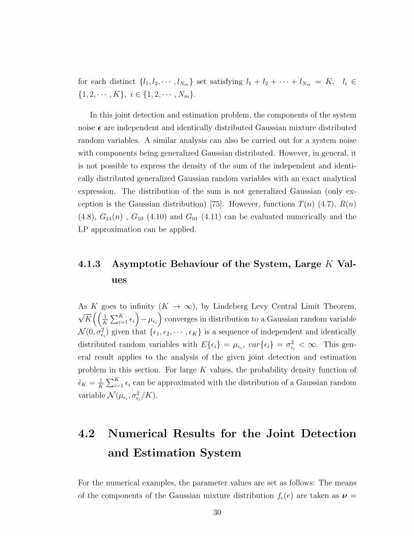
for each distinct {l1, l2, · · · , lNm} set satisfying l1 + l2 + · · · + lNm = K, li ∈{1, 2, · · · , K}, i ∈ {1, 2, · · · , Nm}.

In this joint detection and estimation problem, the components of the system

noise ε are independent and identically distributed Gaussian mixture distributed

random variables. A similar analysis can also be carried out for a system noise

with components being generalized Gaussian distributed. However, in general, it

is not possible to express the density of the sum of the independent and identi-

cally distributed generalized Gaussian random variables with an exact analytical

expression. The distribution of the sum is not generalized Gaussian (only ex-

ception is the Gaussian distribution) [75]. However, functions T (n) (4.7), R(n)

(4.8), G11(n) , G10 (4.10) and G01 (4.11) can be evaluated numerically and the

LP approximation can be applied.

4.1.3 Asymptotic Behaviour of the System, Large K Val-

ues

As K goes to infinity (K → ∞), by Lindeberg Levy Central Limit Theorem,√K((

1K

∑Ki=1 εi

)−µεi

)converges in distribution to a Gaussian random variable

N (0, σ2εi

) given that {ε1, ε2, · · · , εK} is a sequence of independent and identically

distributed random variables with E{εi} = µεi , var{εi} = σ2εi< ∞. This gen-

eral result applies to the analysis of the given joint detection and estimation

problem in this section. For large K values, the probability density function of

εK = 1K

∑Ki=1 εi can be approximated with the distribution of a Gaussian random

variable N (µεi , σ2εi/K).

4.2 Numerical Results for the Joint Detection

and Estimation System

For the numerical examples, the parameter values are set as follows: The means

of the components of the Gaussian mixture distribution fε(e) are taken as ν =

30

[0.40 0.15 0.45]. The weights of the components are µ = [5.25 −0.5 −4.5]. The

standard deviations of the components are equal to each other, and this value

is considered as the variable to evaluate the performance of noise enhancement

for different signal-to-noise (SNR) values. The defined decision rule (4.2) is a

threshold detector, where τPF is set for different standard deviation values such

that the false alarm rate of the given system is equal to 0.15 (constant false alarm

rate). Regarding (4.6), the mean parameter a is 4.5 and the standard deviation

b is 1.25. The estimator is unbiased for the considered scenario. 0-1 Estimation

Cost Function parameter 4 is taken as 0.75.

The optimization problem in (2.19) aims to minimize the conditional estima-

tion risk with respect to the false alarm rate and the detection probability. In this

example, the false alarm constraint α and the detection probability constraint β

are taken respectively as the false alarm rate and the detection probability of the

original system. The support of the additive noise is considered as [−10, 10]. In

this study, a closed form expression of this optimization problem cannot be pre-

sented. However, based on Theorem 1, numerical optimization tools can be used

to find the global solution. Similarly, the LP approximation is also applied on

this example and the results are displayed in the figures and tables. To solve the

global optimization problem and the LP problems, CVX (a package for specifying

and solving convex programs) is used [76,77].

The conditional estimation risk values are plotted versus σ in Figure 4.1 for

K = 1 and in Figure 4.2 for K = 4, in the absence (original) and in the presence

of additive noise. In these figures, it is observed that the system performance

improvement is reduced as the standard deviation σ increases. In other words, the

noise enhancement improvement effect is more effective in the high SNR region.

The improvement is mainly caused by the multimodal nature of the observation

statistics and increasing the standard deviation σ reduces this effect. In both

of the figures, the performances of the LP approximations are also illustrated in

comparison with the global solution of the optimization problem. Noise samples

are taken uniformly from the support of the additive noise with different step size

values.

31

As it is clearly observed from the figure, the accuracy of the LP approximation

is heavily dependent on the step size between the noise samples. The solutions of

the LP approximation (3.8) to the minimization of the conditional estimation risk

optimization problem (3.4) is sufficiently close to the global optimization solution

for step sizes 0.4 (K = 1) and 0.1 (K = 4), which are reasonable values. As it

is clear from Figure 4.2, the performance of the given joint detection system is

superior for K = 4 in comparison to the scalar observation case K = 1. In this

numerical example, the vector case corresponds to taking more samples and an

increase in the signal-to-noise ratio effectively. Similarly, the performances of the

LP approximations are depicted with the original curve and the global solution.

As the number of samples in the LP approximation increases (equivalently, as

the step size interval decreases), it is expected to observe that the LP solution

becomes more similar to the global optimal solution. This is the main intuition

behind the performance degradation in the LP approximation with higher step

size values. The numerical results presented in Figures 4.1 and 4.2 confirm this

assessment. Some numerical values of the conditional estimation risk, detection

probability and false alarm rate of this noise enhanced system are given in Ta-

ble 4.1.

In Figure 4.3, the probability density functions of εk and εK are drawn. As it

is indicated, εk has a Gaussian mixture density with three components. Also, εK

is the sample mean random variable of K independent and identically distributed

εk random variables and it is shown that it has a Gaussian mixture density. In

Figures 4.4, 4.5 and 4.6 the solutions of the optimization problem in (3.4) are

presented for the solutions of the LP problem in (3.8) with different step size

intervals, where the standard deviations of the components of the Gaussian mix-

ture system noise are equal to 0.3 and 0.4. According to Theorem 1, the optimal

solution to the optimization problems (2.19) is a probability mass function with

at most three point masses. The experimental results confirm this proposal. In

these figures, the locations and weights of these point masses are presented.

Notice that Theorem 1 only describes the form of the global optimum solution

to the optimization problem in (2.19). It does not directly apply to the LP prob-

lem in (3.8). Therefore, it can be expected that the optimal λ∗ solutions of the

32

0 0.5 1 1.5 2 2.5 30.55

0.6

0.65

0.7

0.75

0.8

0.85

0.9

0.95

1

Standard Deviation

Co

ndit

ional

Est

imat

ion

Ris

k

Original

Global Solution

LP Step Size = 2

LP Step Size = 1

LP Step Size = 0.2

Figure 4.1: Noise enhancement effects for the minimization of the conditionalestimation risk, K = 1 (NP framework).

0 0.5 1 1.5

0.58

0.6

0.62

0.64

0.66

0.68

0.7

0.72

0.74

Standard Deviation

Cond

itio

nal

Est

imat

ion

Ris

k

Original

Global Solution

LP Step Size = 0.5

LP Step Size = 0.2

LP Step Size = 0.1

Figure 4.2: Noise enhancement effects for the minimization of the conditionalestimation risk, K = 4 (NP framework).

33

−8 −6 −4 −2 0 2 4 6 80

0.1

0.2

0.3

0.4

0.5

0.6

0.7

ε

fǫK(ε)

(a) fεk(ε) density, K = 1

−8 −6 −4 −2 0 2 4 6 80

0.1

0.2

0.3

0.4

0.5

0.6

0.7

ε

fǫK(ε)

(b) fεK (ε) density, K = 4

Figure 4.3: Probability density functions of εk and εK .

σ=0.3, K=1 τPF E{T (0)} E{R(0)} E{G11(0)}E{R(0)} E{T (n)} E{R(n)} E{G11(n)}

E{R(n)}LP (2.0) 5.3456 0.1500 0.4220 0.9533 0.1500 0.4220 0.9376LP (1.0) 5.3456 0.1500 0.4220 0.9533 0.1500 0.4220 0.7796LP (0.2) 5.3456 0.1500 0.4220 0.9533 0.1500 0.4220 0.7694Opt. Sol. 5.3456 0.1500 0.4220 0.9533 0.1500 0.4220 0.7684





Table 4.1: Optimal solutions for the NP based problem (3.4) and the solutionsof the linear fractional programming problem defined in (3.6).

problem (3.8) can have non-zero components other than the three components

which are given in Figures 4.4 and 4.5. However, it is observed for this numerical

example that these non-zero elements are negligible in general and the LP solu-

tions reflect the three mass structure of the global solution. Theorem 1 expresses

that the optimal global solution PMF has at most three distinct point masses.

For this numerical example with K = 4 and σ = 0.4, the global optimal solution

for additive noise probability distribution is a PMF with two point masses and it

is depicted in Figure 4.6. The LP solutions yield similar distributions with two

or three point masses.

34

−6 −4 −2 0 2 4 60

0.05

0.1

0.15

0.2

0.25

0.3

0.35

0.4

0.45

0.5

Locations of the Masses

Wei

ghts

of

the

Mas

ses

LP Step Size = 2

LP Step Size = 1

LP Step Size = 0.2

Global Solution

Figure 4.4: Optimal solutions of the NP problem (3.4) and the solutions of thelinear fractional programming problem defined in (3.6) for K = 1 and σ = 0.3.

−1 −0.5 0 0.5 1 1.5 20

0.1

0.2

0.3

0.4

0.5

0.6

0.7


Wei

gh

ts o

f th

e M

asse

s

LP Step Size = 0.5

LP Step Size = 0.2

LP Step Size = 0.1

Global Solution


35

−1 −0.5 0 0.5 1 1.5 20

0.1

0.2

0.3

0.4

0.5

0.6

0.7


Wei

gh

ts o

f th

e M

asse

s

LP Step Size = 0.5

LP Step Size = 0.2

LP Step Size = 0.1

Global Solution


For the same system noise distribution fεk(ε), the problem in the Bayes de-

tection framework is also evaluated for P (H0) = 0.5 and τ = a/2 in the absence

(original) and presence of additive noise in Figures 4.7 and 4.8 . The Bayes es-

timation risk curves of the LP approximations are also illustrated in comparison

with the global solution. The behavior of the curves are very similar to the results

for the NP detection framework. The noise enhancement improvement effect is

again more effective in the high SNR region. Some numerical values of the Bayes

estimation and Bayes detection risks of both original given and noise enhanced

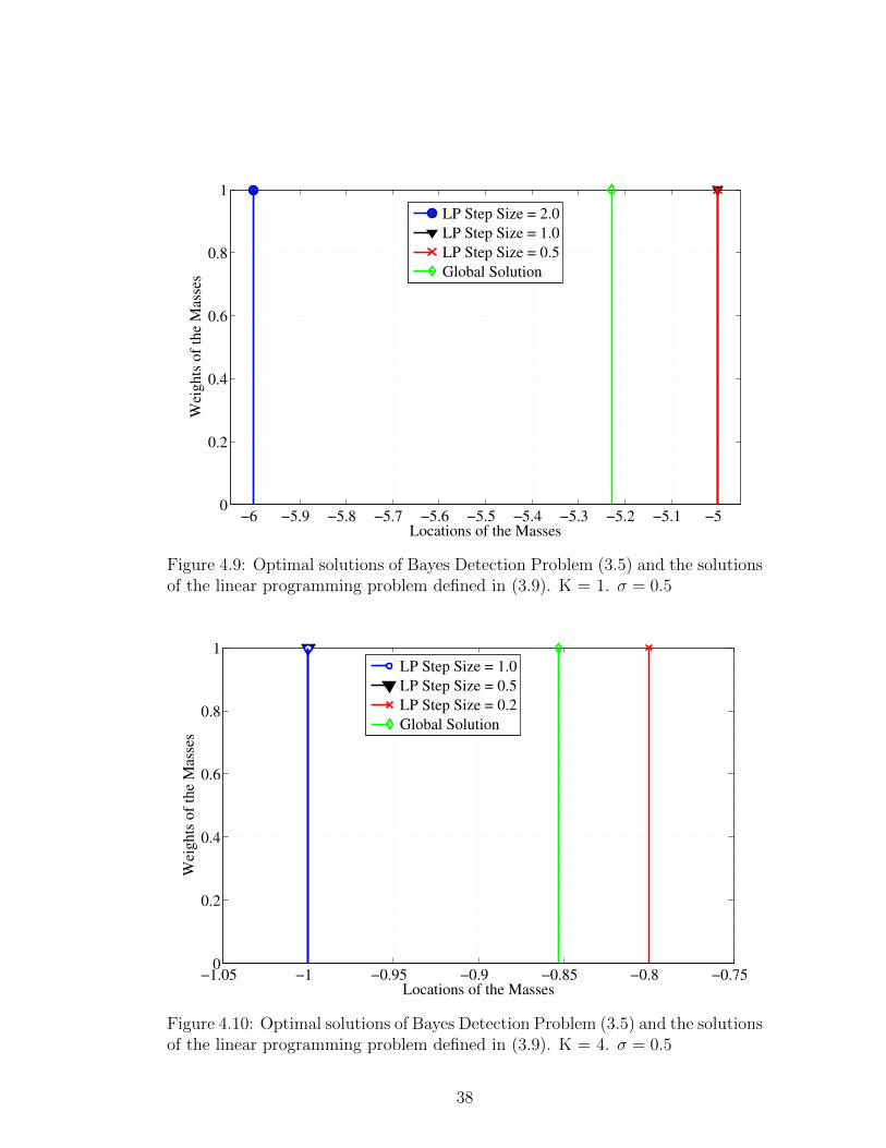
joint systems are given in Table 4.2. In Bayes problem, optimal noise probability

mass functions have one or two mass points. In Figures 4.9 and 4.10, global solu-

tion is a single mass point . In Figure 4.11, global solution has two mass points.

Notice that the LP solution with step size 1.0 is a single mass function at location

0 in this figure. As it can be observed from Table 4.2, LP problem with step size

1.0 is non-improvable and the LP solution is adding zero noise.

36

0 0.5 1 1.5 2 2.5 3 3.5 4 4.5

0.35

0.4

0.45

0.5

0.55

0.6

0.65

0.7

Standard Deviation

Bay

es R

isk

Original

Global Solution

LP Step Size = 2.0

LP Step Size = 1.0

LP Step Size = 0.5

Figure 4.7: Noise enhancement effects for the minimization of the Bayes estima-tion risk, K = 1 (Bayes detection framework).

0 0.2 0.4 0.6 0.8 1 1.2 1.4 1.6 1.8 20.35

0.4

0.45

0.5

Standard Deviation

Bay

es R

isk

Original

Global Solution

LP Step Size = 1.0

LP Step Size = 0.5

LP Step Size = 0.2


37

−6 −5.9 −5.8 −5.7 −5.6 −5.5 −5.4 −5.3 −5.2 −5.1 −50

0.2

0.4

0.6

0.8

1


Wei

ghts

of

the

Mas

ses

LP Step Size = 2.0

LP Step Size = 1.0

LP Step Size = 0.5

Global Solution

Figure 4.9: Optimal solutions of Bayes Detection Problem (3.5) and the solutionsof the linear programming problem defined in (3.9). K = 1. σ = 0.5

−1.05 −1 −0.95 −0.9 −0.85 −0.8 −0.750

0.2

0.4

0.6

0.8

1


Wei

gh

ts o

f th

e M

asse

s

LP Step Size = 1.0

LP Step Size = 0.5

LP Step Size = 0.2

Global Solution


38

−1 −0.5 0 0.50

0.2

0.4

0.6

0.8

1


Wei

ghts

of

the

Mas

ses

LP Step Size = 1.0

LP Step Size = 0.5

LP Step Size = 0.2

Global Solution


σ=0.5, K=1 rx(φ) rx(θ) ry(φ) ry(θ)LP (1.0) 0,1959 0,4757 0.3266 0,4061LP (0.5) 0.4216 0,6514 0.3057 0,3411LP (0.2) 0.4216 0,6514 0.3057 0,3411Opt. Sol. 0.4216 0,6514 0.3088 0,3333

σ=0.5, K=4 rx(φ) rx(θ) ry(φ) ry(θ)LP (1.0) 0,1959 0,4757 0.1956 0,4076LP (0.5) 0,1959 0,4757 0.1956 0,4076LP (0.2) 0,1959 0,4757 0.1899 0,4015Opt. Sol. 0,1959 0,4757 0.1906 0,4005

σ=0.75, K=4 rx(φ) rx(θ) ry(φ) ry(θ)LP (1.0) 0.1933 0,4734 0.1933 0,4734LP (0.5) 0.1933 0,4734 0.1933 0,4514LP (0.2) 0.1933 0,4734 0.1933 0,4372Opt. Sol. 0.1933 0,4734 0.1933 0,4357

Table 4.2: Optimal solutions of Bayes detection framework problem (3.5) and thesolutions of the linear programming problem defined in (3.9).

39

A different NP detection framework is also analyzed for µ = [−3.8 − 1.6 −0.54 0.50 2.42 4.3], ν = [0.33 0.13 0.08 0.07 0.11 0.28], a = 5, b = 1, 4 = 1,

and a constant false alarm rate of 0.1. The results are depicted in Figure 4.12.

Another different Bayes detection framework problem is also analyzed for ν =

[0.25 0.50 0.25], µ = [3 − 0.5 − 2], a = 3, b = 1, τ = a/2, 4 = 0.5, and

P (H0) = 0.5 in Figure 4.13 for K = 1.

40

0 0.2 0.4 0.6 0.8 1 1.2 1.4 1.60.55

0.6

0.65

0.7

0.75

0.8

0.85

0.9

Standard Deviation

Con

dit

ional

Est

imat

ion

Ris

k

Original

Global Solution

LP (Step Size = 1)

LP (Step Size = 0.5)


Figure 4.12: Noise enhancement effects for the minimization of the conditionalestimation risk, K = 1 (NP detection framework).

0 0.5 1 1.5

0.35

0.4

0.45

0.5

0.55

0.6

Standard Deviation

Bay

es R

isk

Original

Global Solution

LP (Step Size = 1)




41

Chapter 5

Conclusion

In this thesis, to improve the performance of a given joint detection and estima-

tion system, the injection of an independent random variable (additive noise) to

the system has been considered. The statistical properties of the joint detection

and estimation system have been analyzed in two different detection frameworks:

Bayesian and NP. In non-Gaussian environments, the optimal detection, estima-

tion, or joint detection-estimation systems are generally complicated (possibly

cannot be expressed in closed form). This may motivate the implementation of

suboptimal systems and performance loss. This study shows that noise benefits

in joint detection and estimation systems can be realized to improve the perfor-

mances of given suboptimal and relatively simple joint detection and estimation

systems, which are for example optimal in Gaussian background noise and expe-

rience heavy performance degradation in a non-Gaussian environment.

For both NP and Bayesian detection frameworks, the optimal additive noise

probability distributions have been found to be discrete (i.e., PMFs). With this

result, the search for the optimal additive noise has been considerably simpli-

fied and can be solved by using global optimization techniques. However, the

optimization problem is still not convex in general. In order to overcome possi-

ble complexities regarding the solution of the proposed problem, an LP problem

approximation has been proposed. This sampling operation in additive noise ran-

dom variable support set results in a performance degradation in comparison to

42

the global optimal solution. The evaluation of numerical examples has indicated

that this performance loss is negligible if the step size between the samples is

chosen adequately. With this observation, under both NP and Bayes detection

frameworks, it can be expressed that the LP approximation is well-suited for re-

alistic scenarios. This should be noted as an important observation to justify the

applicability of the noise enhanced systems in real life scenarios since it is less

complex than finding a global solution to the presented optimization problems.

The noise enhancement idea may draw some criticism as the solution of the

proposed optimization problems in (3.4) and (3.5) can require heavy computa-

tion. However, the LP approximation idea significantly reduces the computational

load. One can assume that when the probability distributions of the observations

are fixed, the LP solutions can be computed beforehand and stored. However,

pre-computation is not always efficient and an adaptive methodology is needed

especially if the background noise is time varying. Future work can focus on de-

veloping an adaptive algorithm to find a near optimal additive noise distribution

under LP approximation while the joint detection and estimation is running in

real time.

43

Bibliography

[1] M. D. McDonnell, “Is electrical noise useful? [point of view],” Proc. IEEE,

vol. 99, pp. 242–246, Feb. 2011.

[2] M. D. McDonnell and D. Abbott, “What is stochastic resonance? definitions,

misconceptions, debates, and its relevance to biology,” PLoS Comput Biol,

vol. 5, p. e1000348, 05 2009.

[3] R. Benzi, A. Sutera, and A. Vulpiani, “The mechanism of stochastic reso-

nance,” Journal of Physics A: Mathematical and General, vol. 14, no. 11,

p. L453, 1981.

[4] B. McNamara and K. Wiesenfeld, “Theory of stochastic resonance,” Phys.

Rev. A, vol. 39, pp. 4854–4869, May 1989.

[5] L. Schuchman, “Dither signals and their effect on quantization noise,” IEEE

Trans. Commun. Technol., vol. 12, pp. 162–165, December 1964.

[6] L. Gammaitoni, “Stochastic resonance and the dithering effect in threshold

physical systems,” Phys. Rev. E, vol. 52, pp. 4691 – 4698, 1995.

[7] R. A. Wannamaker, S. P. Lipshitz, and J. Vanderkooy, “Stochastic resonance

as dithering,” Phys. Rev. E, vol. 61, pp. 233–236, Jan 2000.

[8] A. Longtin, “Stochastic resonance in neuron models,” Journal of Statistical

Physics, vol. 70, no. 1-2, pp. 309–327, 1993.

[9] M. C. Mahato and S. R. Shenoy, “Hysteresis loss and stochastic resonance: A

numerical study of a double-well potential,” Phys. Rev. E, vol. 50, pp. 2503–

2512, Oct 1994.

44

[10] A. R. Bulsara and A. Zador, “Threshold detection of wideband signals: A

noise-induced maximum in the mutual information,” Phys. Rev. E, vol. 54,

pp. R2185–R2188, Sep 1996.

[11] C. Heneghan, C. C. Chow, J. J. Collins, T. T. Imhoff, S. B. Lowen, and M. C.

Teich, “Information measures quantifying aperiodic stochastic resonance,”

Phys. Rev. E, vol. 54, pp. R2228–R2231, Sep 1996.

[12] C. C. Chow, T. T. Imhoff, and J. J. Collins, “Enhancing aperiodic stochas-

tic resonance through noise modulation,” Chaos: An Interdisciplinary J. of

Nonlinear Sci., vol. 8, no. 3, 1998.

[13] A. Neiman, L. Schimansky-Geier, F. Moss, B. Shulgin, and J. J. Collins,

“Synchronization of noisy systems by stochastic signals,” Phys. Rev. E,

vol. 60, pp. 284–292, Jul 1999.

[14] G. C. Kember, G. A. Fenton, K. Collier, and J. A. Armour, “Aperiodic

stochastic resonance in a hysteretic population of cardiac neurons,” Phys.

Rev. E, vol. 61, pp. 1816–1824, Feb 2000.

[15] J. Li and L. Zeng, “Stochastic resonance in a bistable system subject to

multi-time-delayed feedback and aperiodic signal,” Journal of Physics A:

Mathematical and Theoretical, vol. 43, no. 49, p. 495002, 2010.

[16] N. G. Stocks, “Suprathreshold stochastic resonance in multilevel threshold

systems,” Phys. Rev. Lett., vol. 84, pp. 2310–2313, Mar 2000.

[17] N. G. Stocks, “Information transmission in parallel threshold arrays:

Suprathreshold stochastic resonance,” Phys. Rev. E, vol. 63, p. 041114, Mar

2001.

[18] D. Rousseau and F. Chapeau-Blondeau, “Suprathreshold stochastic res-

onance and signal-to-noise ratio improvement in arrays of comparators,”

Physics Letters A, vol. 321, no. 56, pp. 280 – 290, 2004.

[19] P.-O. Amblard, S. Zozor, M. D. McDonnell, and N. G. Stocks, “Pooling

networks for a discrimination task: noise-enhanced detection,” vol. 6602,

pp. 66020S–66020S–12, 2007.

45

[20] A. Patel and B. Kosko, “Optimal mean-square noise benefits in quantizer-

array linear estimation,” IEEE Sig. Process. Lett., vol. 17, pp. 1005–1009,

Dec 2010.

[21] Y. Guo and J. Tan, “Suprathreshold stochastic resonance in multilevel

threshold system driven by multiplicative and additive noises,” Commun.

Nonlinear Sci Numer Simulat, vol. 18, no. 10, pp. 2852 – 2858, 2013.

[22] Q. Li and Z. Li, “A novel sequential spectrum sensing method in cognitive

radio using suprathreshold stochastic resonance,” IEEE Trans. Veh. Tech.,

vol. 63, pp. 1717–1725, May 2014.

[23] F. Chapeau-Blondeau, “Stochastic resonance and optimal detection of pulse

trains by threshold devices,” Digit. Signal Process., vol. 9, no. 3, pp. 162 –

177, 1999.

[24] S. Sugiura, A. Ichiki, and Y. Tadokoro, “Stochastic-resonance based iterative

detection for serially-concatenated turbo codes,” IEEE Sig. Process. Lett.,

vol. 19, pp. 655–658, Oct 2012.

[25] D. He, “Chaotic stochastic resonance energy detection fusion used in coop-

erative spectrum sensing,” IEEE Trans. Veh. Tech., vol. 62, pp. 620–627,

Feb 2013.

[26] A. Patel and B. Kosko, “Noise benefits in quantizer-array correlation detec-

tion and watermark decoding,” IEEE Trans. Sig. Process., vol. 59, pp. 488–

505, Feb. 2011.

[27] M. E. Inchiosa and A. R. Bulsara, “Signal detection statistics of stochastic

resonators,” Phys. Rev. E, vol. 53, pp. R2021–R2024, Mar 1996.

[28] F. Chapeau-Blondeau, “Noise-aided nonlinear bayesian estimation,” Phys.

Rev. E, vol. 66, p. 032101, Sep 2002.

[29] F. Chapeau-Blondeau and D. Rousseau, “Noise-enhanced performance for an

optimal bayesian estimator,” IEEE Trans. Sig. Process., vol. 52, pp. 1327–

1334, May 2004.

46

[30] A. A. Saha and G. Anand, “Design of detectors based on stochastic reso-

nance,” Signal Process., vol. 83, no. 6, pp. 1193 – 1212, 2003.

[31] D. Rousseau and F. Chapeau-Blondeau, “Stochastic resonance and improve-

ment by noise in optimal detection strategies,” Digit. Signal Process., vol. 15,

pp. 19–32, Jan. 2005.

[32] D. Rousseau, G. Anand, and F. Chapeau-Blondeau, “Noise-enhanced non-

linear detector to improve signal detection in non-Gaussian noise,” Signal

Process., vol. 86, no. 11, pp. 3456 – 3465, 2006. Special Section: Distributed

Source Coding.

[33] Y. Wang, “Nonlinear statistics to improve signal detection in generalized

Gaussian noise,” Digit. Signal Process., vol. 18, no. 3, pp. 444 – 449, 2008.

[34] F. Chapeau-Blondeau and D. Rousseau, “Raising the noise to improve per-

formance in optimal processing,” J. Stat. Mech., vol. 2009, no. 01, p. P01003,

2009.

[35] F. Duan and B. Xu, “Parameter-induced stochastic resonance and baseband

binary PAM signals transmission over an AWGN channel,” Int. J.of Bifur-

cation and Chaos, vol. 13, no. 02, pp. 411–425, 2003.

[36] B. Xu, F. Duan, and F. m. c. Chapeau-Blondeau, “Comparison of aperiodic

stochastic resonance in a bistable system realized by adding noiseand by

tuning system parameters,” Phys. Rev. E, vol. 69, p. 061110, Jun 2004.

[37] S. Jiang, F. Guo, Y. Zhou, and T. Gu, “Parameter-induced stochastic reso-

nance in an over-damped linear system,” Physica A, vol. 375, no. 2, pp. 483

– 491, 2007.

[38] Q. He and J. Wang, “Effects of multiscale noise tuning on stochastic reso-

nance for weak signal detection,” Digit. Signal Process., vol. 22, no. 4, pp. 614

– 621, 2012.

[39] Y. Tadokoro and A. Ichiki, “A simple optimum nonlinear filter for stochastic-

resonance-based signal detection,” in Proc. IEEE Int. Conf. Acoust., Speech,

Signal Process. (ICASSP), pp. 5760–5764, May 2013.

47

[40] S. Kay, “Can detectability be improved by adding noise?,” IEEE Sig. Pro-

cess. Lett., vol. 7, pp. 8–10, Jan 2000.

[41] S. Kay, J. Michels, H. Chen, and P. Varshney, “Reducing probability of

decision error using stochastic resonance,” IEEE Sig. Process. Lett., vol. 13,

pp. 695–698, Nov 2006.

[42] O. Osoba, S. Mitaim, and B. Kosko, “The noisy expectation – maximization

algorithm,” Fluctuation and Noise Lett., vol. 12, no. 03, p. 1350012, 2013.

[43] H. Chen, P. K. Varshney, J. H. Michels, and S. M. Kay, “Theory of the

stochastic resonance effect in signal detection: Part I — Fixed detectors,”

IEEE Trans. Sig. Process., vol. 55, pp. 3172–3184, July 2007.

[44] S. Kay, “Noise enhanced detection as a special case of randomization,” IEEE

Sig. Process. Lett., Nov. 2008.

[45] H. Chen, P. K. Varshney, and J. H. Michels, “Noise enhanced parameter

estimation,” IEEE Trans. Sig. Process., vol. 56, pp. 5074–5081, Oct. 2008.

[46] H. Chen and P. Varshney, “Theory of the stochastic resonance effect in signal

detection: Part II — Variable Detectors,” IEEE Trans. Sig. Process., vol. 56,

pp. 5031–5041, Oct 2008.

[47] H. Chen, P. Varshney, and J. Michels, “Improving sequential detection

performance via stochastic resonance,” IEEE Sig. Process. Lett., vol. 15,

pp. 685–688, 2008.

[48] H. Chen, P. Varshney, S. Kay, and J. Michels, “Noise enhanced nonpara-

metric detection,” IEEE Trans. Inform. Theory, vol. 55, pp. 499–506, Feb

2009.

[49] A. Patel and B. Kosko, “Optimal noise benefits in neyman pearson and

inequality-constrained statistical signal detection,” IEEE Trans. Sig. Pro-

cess., May 2009.

[50] S. Bayram and S. Gezici, “On the improvability and nonimprovability of

detection via additional independent noise,” IEEE Sig. Process. Lett., vol. 16,

pp. 1001–1004, Nov 2009.

48

[51] S. Bayram, S. Gezici, and H. V. Poor, “Noise enhanced hypothesis-testing

in the restricted bayesian framework,” IEEE Trans. Sig. Process., vol. 58,

pp. 3972–3989, Aug. 2010.

[52] W. Chen, J. Wang, H. Li, and S. Li, “Stochastic resonance noise en-

hanced spectrum sensing in cognitive radio networks,” in Proc. IEEE Global

Telecommun. Conf. (GLOBECOM), pp. 1–6, Dec 2010.

[53] G. Balkan and S. Gezici, “CRLB based optimal noise enhanced parameter

estimation using quantized observations,” IEEE Sig. Process. Lett., vol. 17,

pp. 477–480, May 2010.

[54] S. Bayram, N. D. Vanli, B. Dulek, I. Sezer, and S. Gezici, “Optimum power

allocation for average power constrained jammers in the presence of non-

Gaussian noise,” IEEE Commun. Lett., vol. 16, pp. 1153–1156, August 2012.

[55] S. Bayram and S. Gezici, “Stochastic resonance in binary composite

hypothesis-testing problems in the neyman-pearson framework,” Digit. Sig-

nal Process., vol. 22, pp. 391–406, May 2012.

[56] J.-Y. Liu and Y.-T. Su, “Noise-enhanced blind multiple error rate estimators

in wireless relay networks,” IEEE Trans. Veh. Tech., vol. 61, pp. 1145–1161,

March 2012.

[57] A. Vempaty, V. Nadendla, and P. Varshney, “Further results on noise-

enhanced distributed inference in the presence of byzantines,” in Proc. 16th

International Symposium on Wireless Personal Multimedia Communications

(WPMC), pp. 1–5, June 2013.

[58] G. Guo, X. Yu, Y. Jing, and M. Mandal, “Optimal design of noise-enhanced

binary threshold detector under AUC measure,” IEEE Sig. Process. Lett.,

vol. 20, pp. 161–164, Feb 2013.

[59] S. Zhang, J. Wang, and S. Li, “Adaptive bistable stochastic resonance aided

spectrum sensing,” in Proc IEEE Int. Conf. on Commun. (ICC), pp. 2622–

2626, June 2013.

49

[60] S. Bayram, S. Gultekin, and S. Gezici, “Noise enhanced hypothesis-testing

according to restricted neymanpearson criterion,” Digit. Signal Process.,

vol. 25, pp. 17 – 27, Feb. 2014.

[61] S. Bayram and S. Gezici, “On the performance of single-threshold detectors

for binary communications in the presence of Gaussian mixture noise,” IEEE

Trans. Comm., vol. 58, pp. 3047–3053, November 2010.

[62] G. V. Moustakides, G. H. Jajamovich, A. Tajer, and X. Wang, “Joint detec-

tion and estimation: Optimum tests and applications,” IEEE Trans. Inform.

Theory, July 2012.

[63] H. V. Poor, An Introduction to Signal Detection and Estimation. New York:

Springer-Verlag, 1994.

[64] T. M. Cover and J. A. Thomas, Elements of information theory. John Wiley

& Sons, 2012.

[65] A. B. Akbay and S. Gezici, “Noise enhancement in joint detection and es-

timation systems,” in Proc. Signal Process. and Commun. Applicat. Conf.

(SIU), pp. 1059–1062, April 2014.

[66] P. Whittle, Probability Via Expectation. New York: Springer-Verlag, 1992.

[67] D. P. Bertsekas, A. Nedic, and A. E. Ozdaglar, Convex Analysis and Op-

timization. Athena Scientific optimization and computation series, Boston,

MA: Athena Scientific, 2003.

[68] K. E. Parsopoulos and M. N. Vrahatis, Particle swarm optimization method

for constrained optimization problems, pp. 214–220. IOS Press, 2002. in

Intelligent Technologies–Theory and Applications: New Trends in Intelligent

Technologies.

[69] A. I. F. Vaz and E. M. G. P. Fernandes, “Optimization of nonlinear con-

strained particle swarm,” Baltic Journal on Sustainability, vol. 12, no. 1,

pp. 30–36, 2006.

[70] S. P. Boyd and L. Vandenberghe, Convex Optimization. Cambridge, UK:

Cambridge University Press, 2004.

50

[71] V. Bhatia and B. Mulgrew, “Non-parametric likelihood based channel esti-

mator for Gaussian mixture noise,” Signal Process., vol. 87, no. 11, pp. 2569

– 2586, 2007.

[72] C. Luschi and B. Mulgrew, “Nonparametric trellis equalization in the pres-

ence of non-Gaussian interference,” IEEE Trans. Comm., vol. 51, pp. 229–

239, Feb 2003.

[73] A. Banerjee, P. Burlina, and R. Chellappa, “Adaptive target detection in

foliage-penetrating sar images using alpha-stable models,” IEEE Trans. Im-

age Process., vol. 8, pp. 1823–1831, Dec 1999.

[74] M. Bouvet and S. Schwartz, “Comparison of adaptive and robust receivers

for signal detection in ambient underwater noise,” IEEE Trans. Acoust.,

Speech, Signal Process., vol. 37, pp. 621–626, May 1989.

[75] Q. Zhao, H. wei Li, and Y. tong Shen, “On the sum of generalized Gaussian

random signals,” in Proc. Int. Conf. Signal Proc. (ICSP), vol. 1, pp. 50–53

vol.1, Aug 2004.

[76] I. CVX Research, “CVX: Matlab software for disciplined convex program-

ming, version 2.0.” http://cvxr.com/cvx, Aug. 2012.

[77] M. Grant and S. Boyd, “Graph implementations for nonsmooth convex pro-

grams,” in Recent Advances in Learning and Control (V. Blondel, S. Boyd,

and H. Kimura, eds.), Lecture Notes in Control and Information Sciences,

pp. 95–110, Springer-Verlag Limited, 2008. http://stanford.edu/~boyd/

graph_dcp.html.

[78] I. S. Gradshteyn and I. M. Ryzhik, Table of Integrals, Series, and Products

(7th Edition). Elsevier/Academic Press, Amsterdam, 2007.

[79] A. Leon-Garcia, Probability and Random Processes For EE’s (3rd Edition).

Upper Saddle River, NJ, USA: Prentice-Hall, Inc., 2007.

[80] M. Abramowitz and I. Stegun, Handbook of Mathematical Functions: with

Formulas, Graphs, and Mathematical Tables. Dover Books on Mathematics,

Dover Publications, 2012.

51

Appendix A

Derivation of Conditional

Estimation Risks

The equation (2.8) is already stated in [62] as the relation (7) without any deriva-

tion. In this section, it is demonstrated that the estimation performance criterion

is the average Bayes risk conditioned on true hypothesis H1 and decision H1. The

estimation performance criterion of the joint detection and estimation system is

proposed as

E{c(Θ, θ(X))|H1, H1} =

∫Λ

∫RK

c(θ, θ(x))fX(θ,x|H1, H1) dxdθ (A.1)

where f(θ,x|H1, H1) is the joint probability density function of the observation

X and estimated parameter Θ. It can be expressed as

f(θ,x|H1, H1) = f(x|θ,H1, H1)π(θ|H1, H1) (A.2)

Also,

fX(x|θ,H1, H1) =fX(x, H1|θ,H1)

P (H1|θ,H1)=P (H1|θ,H1,x)f(x|θ,H1)

P (H1|θ,H1)=φ(x)fX1 (x|θ)

P (H1|θ,H1)(A.3)

Note that fX(x|θ,H1) is previously denoted as fX1 (x|θ) in (2.1). The probabil-

ity of deciding in favor of H1 is the detector function when the observation is

52

given. Providing additional information does not change this probability; hence

P (H1|θ,H1,x) = φ(x). In addition,

π(θ|H1, H1) =π(θ, H1|H1)

P (H1|H1)=P (H1|θ,H1)π(θ|H1)

P (H1|H1). (A.4)

Inserting (A.2), (A.3), and (A.4) into (A.1) gives the conditional Bayes risk

(Equation (7) in [62]):

E{C(Θ, θ(X))|H1, H1} =

∫Λ

∫RK

C(θ, θ(x))φ(x)fX1 (x|θ)π(θ) dxdθ

P (H1|H1)(A.5)

Similarly, the derivation of the conditional estimation risk after noise addition

(2.15) is also presented below:

E{c(Θ, θ(Y ))|H1, H1} =

∫Λ

∫RK

c(θ, θ(y))fY (θ,y|H1, H1) dydθ. (A.6)

Applying the same approach, the probability density of Y conditioned on true

hypothesis H1, decision H1 and parameter Θ can be obtained as follows:

fY (y|θ,H1, H1) =φ(y)fY1 (y|θ)

P (H1|θ,H1). (A.7)

Since Y is the summation of two independent random variables, its probability

distribution conditioned on true hypothesis H1 and parameter Θ is given by

fY1 (y|θ) =

∫RK

fN(n)fX1 (y−n|θ) dn . (A.8)

Inserting equations (A.4), (A.7), and (A.8) into (A.6) gives the conditional

estimation risk (2.15) in the presence of additive noise:

J(φ, θ) =

∫RK

fN(n)∫Λ

∫RK

c(θ, θ(y))φ(y)π(θ)fX1 (y−n|θ) dydθdn∫RK

fN(n)∫Λ

∫RK

φ(y)π(θ)fX1 (y−n|θ) dydθdn. (A.9)

53

Appendix B

Derivation of Auxiliary Functions

In this chapter, the derivation of the auxiliary function G11(n) is presented for

the scalar case K = 1. G01 (4.11) can also be derived in a similar way, and

therefore its derivation is not included. As defined in Section 4.1, system noise

ε is Gaussian mixture distributed and parameter θ is Gaussian distributed. For

notational simplicity introduce fX1,i(y − n|θ) = 1√2πσ2

exp(− (y−n−µi−θ)2

2σ2

). Then,

G11(n) is calculated as follows:

G11(n) =

∫Λ

∫R

c(θ, θ(y))φ(y)π(θ)fX1 (y − n|θ) dydθ

=Nm∑i=1

νi

+∞∫−∞

+∞∫−∞

c(θ, θ(y))φ(y)π(θ)fX1,i(y − n|θ)dydθ

=Nm∑i=1

νi

{ τ−4∫−∞

π(θ)

+∞∫τ

fX1,i(y − n|θ)dydθ +

τ+4∫τ−4

π(θ)

+∞∫θ+4

fX1,i(y − n|θ)dydθ

+

+∞∫τ+4

π(θ)

θ−4∫τ

fX1,i(y − n|θ)dydθ +

+∞∫τ+4

π(θ)

+∞∫θ+4

fX1,i(y − n|θ)dydθ

}

54

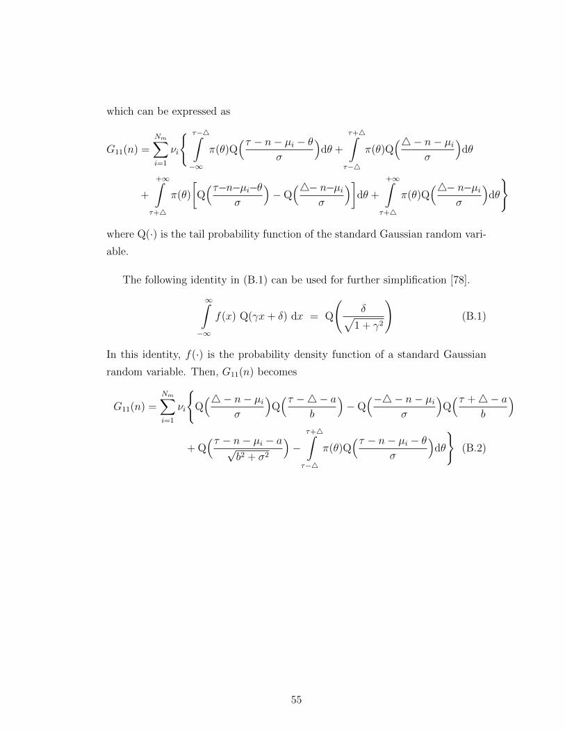
which can be expressed as

G11(n) =Nm∑i=1

νi

{ τ−4∫−∞

π(θ)Q(τ − n− µi − θ

σ

)dθ +

τ+4∫τ−4

π(θ)Q(4− n− µi

σ

)dθ

+

+∞∫τ+4

π(θ)

[Q(τ−n−µi−θ

σ

)−Q

(4− n−µiσ

)]dθ +

+∞∫τ+4

π(θ)Q(4− n−µi

σ

)dθ

}

where Q(·) is the tail probability function of the standard Gaussian random vari-

able.

The following identity in (B.1) can be used for further simplification [78].

∞∫−∞

f(x) Q(γx+ δ) dx = Q

(δ√

1 + γ2

)(B.1)

In this identity, f(·) is the probability density function of a standard Gaussian

random variable. Then, G11(n) becomes

G11(n) =Nm∑i=1

νi

{Q(4− n− µi

σ

)Q(τ −4− a

b

)−Q

(−4− n− µiσ

)Q(τ +4− a

b

)

+ Q(τ − n− µi − a√

b2 + σ2

)−

τ+4∫τ−4

π(θ)Q(τ − n− µi − θ

σ

)dθ

}(B.2)

55

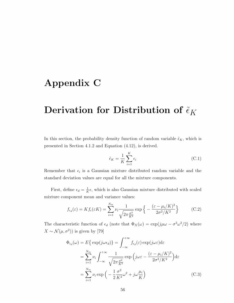
Appendix C

Derivation for Distribution of εK

In this section, the probability density function of random variable εK , which is

presented in Section 4.1.2 and Equation (4.12), is derived.

εK =1

K

K∑i=1

εi (C.1)

Remember that εi is a Gaussian mixture distributed random variable and the

standard deviation values are equal for all the mixture components.

First, define εd = 1Kε, which is also Gaussian mixture distributed with scaled

mixture component mean and variance values:

fεd(ε) = Kfε(εK) =Nm∑i=1

νi1√

2π σ2

K2

exp{− (ε− µi/K)2

2σ2/K2

}(C.2)

The characteristic function of εd (note that ΦX(ω) = exp(jµω − σ2ω2/2) where

X ∼ N (µ, σ2)) is given by [79]

Φεd(ω) = E{

exp(jωεd)} =

∫ +∞

−∞fεd(ε) exp(jωε)dε

=Nm∑i=1

νi

∫ +∞

−∞

1√2π σ2

K2

exp(jωε− (ε− µi/K)2

2σ2/K2

)dε

=Nm∑i=1

νi exp(− 1

2

σ2

K2ω2 + jω

µiK

)(C.3)

56

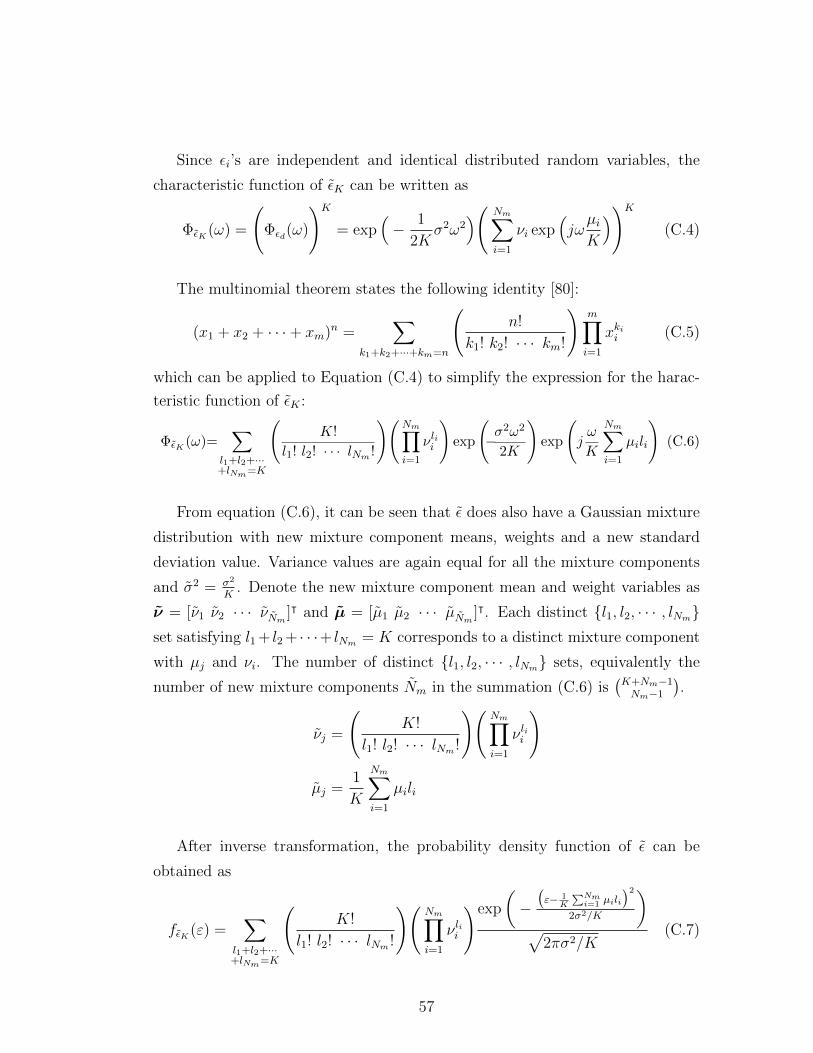
Since εi’s are independent and identical distributed random variables, the

characteristic function of εK can be written as

ΦεK (ω) =

(Φεd(ω)

)K

= exp(− 1

2Kσ2ω2

)( Nm∑i=1

νi exp(jωµiK

))K

(C.4)

The multinomial theorem states the following identity [80]:

(x1 + x2 + · · ·+ xm)n =∑

k1+k2+···+km=n

(n!

k1! k2! · · · km!

)m∏i=1

xkii (C.5)

which can be applied to Equation (C.4) to simplify the expression for the harac-

teristic function of εK :

ΦεK (ω)=∑

l1+l2+···+lNm=K

(K!

l1! l2! · · · lNm !

)(Nm∏i=1

νlii

)exp

(−σ

2ω2

2K

)exp

(jω

K

Nm∑i=1

µili

)(C.6)

From equation (C.6), it can be seen that ε does also have a Gaussian mixture

distribution with new mixture component means, weights and a new standard

deviation value. Variance values are again equal for all the mixture components

and σ2 = σ2

K. Denote the new mixture component mean and weight variables as

ν = [ν1 ν2 · · · νNm]ᵀ and µ = [µ1 µ2 · · · µNm

]ᵀ. Each distinct {l1, l2, · · · , lNm}set satisfying l1 + l2 + · · ·+ lNm = K corresponds to a distinct mixture component

with µj and νi. The number of distinct {l1, l2, · · · , lNm} sets, equivalently the

number of new mixture components Nm in the summation (C.6) is(K+Nm−1Nm−1

).

νj =

(K!

l1! l2! · · · lNm !

)(Nm∏i=1

νlii

)

µj =1

K

Nm∑i=1

µili

After inverse transformation, the probability density function of ε can be

obtained as

fεK (ε) =∑

l1+l2+···+lNm=K

(K!

l1! l2! · · · lNm !

)(Nm∏i=1

νlii

)exp

(−(ε− 1

K

∑Nmi=1 µili

)22σ2/K

)√

2πσ2/K(C.7)

57

Documents

NOISE BENEFITS IN JOINT DETECTION AND ESTIMATION SYSTEMS · NOISE BENEFITS IN JOINT DETECTION AND ESTIMATION SYSTEMS ... NOISE BENEFITS IN JOINT DETECTION AND ... 2.1 Joint detection