Noise Characteristics of MEMS Gyro's Null Drift and Temperature Compensation

Noise Characteristics of MEMS Gyro’s Null Drift and

Temperature Compensation

Jaw-Kuen Shiau*, Chen-Xuan Huang and Ming-Yu Chang

Department of Aerospace Engineering, Tamkang University,

Tamsui, Taiwan 251, R.O.C.

Abstract

Gyroscope is one of the primary sensors for air vehicle navigation and controls. This paper

investigates the noise characteristics of microelectromechanical systems (MEMS) gyroscope null drift

and temperature compensation. This study mainly focuses on temperature as a long-term error source.

An in-house-designed inertial measurement unit (IMU) is used to perform temperature effect testing in

the study. The IMU is placed into a temperature control chamber. The chamber temperature is

controlled to increase from 25 �C to 80 �C at approximately 0.8 degrees per minute. After that, the

temperature is decreased to -40 �C and then returns to 25 �C. The null voltage measurements clearly

demonstrate the rapidly changing short-term random drift and slowly changing long-term drift due to

temperature variations. The characteristics of the short-term random drifts are analyzed and

represented in probability density functions. A temperature calibration mechanism is established by

using an artificial neural network to compensate the long-term drift. With the temperature calibration,

the attitude computation problem due to gyro drifts can be improved significantly.

Key Words: MEMS Gyroscope, Null Drift, Inertial Measurement Unit, Temperature Compensation

1. Introduction

The effectiveness of navigation and controls of an

air vehicle are highly dependent on the degree of pre-

cision of the on-board inertial measurement unit (IMU).

A gyroscope is one of the primary sensors that comprises

the IMU. Traditional units, such as gimbaled gyroscopes,

laser gyroscopes, and fiber-optic gyroscopes provide

high-precision angular rate information for navigation

and control systems [1]. However, they are expensive

and bulky. With the maturation and advancement of

semi-conductor manufacturing technology, MEMS ap-

plication has shifted to non-military purposes in the re-

gular consumer market. As MEMS sensors become

cheaper, smaller, and consume less power, they are in-

creasingly used in flight attitude calculations of un-

manned aerial vehicles (UAVs) [2,3]. This study uses the

low-cost MEMS IMU unit as the basis of this research.

Due to manufacturing limitations, signal drift often

accompanies MEMS gyros. As the calculation of atti-

tude angles requires angular velocity measurements for

integral calculation, the error caused by MEMS gyro

drift increases with time, leading to decreased accuracy.

Thus, drift data processing is extremely important. Gyro

drift is caused by multiple factors and has complex non-

linear characteristics. Therefore, it cannot be clearly ex-

pressed through a single function. Due to various error

sources, the performance characteristics of low-cost gy-

roscopes cause usage limitations [4�7]. According to the

spectral signature, these errors can be categorized into

the more rapidly changing short-term noise and more

slowly changing long-term noise [7]. These error sources

cause basic limitations to solely using gyroscopes for

attitude determination [8,9].

Several methods may be used to process drift-signals

to remove short-term error. However, they are complex

Journal of Applied Science and Engineering, Vol. 15, No. 3, pp. 239�246 (2012) 239

*Corresponding author. E-mail: [email protected]

and time-consuming and thus cannot be easily applied to

real-time and on-line systems [7,10]. To obtain more ac-

curate attitude measurements, recent literature identified

a random drift model of MEMS gyroscope [11,12]. To

simplify its predicted error, the wavelet multi-scale an-

alysis method decomposes the gyroscope random drift

data and constructs a series of gyroscope drift data and

models with different scales. In [12] an adaptive Kalman

filter algorithm is proposed to perform compensation for

random drift noise of gyroscope. As artificial neural net-

works (ANNs) have the ability to approach complex

non-linear functions [13,14], it was used to model the

random drift or temperature drift of gyroscopes [15,16].

Modeling of the random drift of MEMS gyroscope with

neural network is presented in [15]. In [16], a grey radial

basis function neural network is used to model the tem-

perature drift of optical gyroscopes.

Gyro drift is the primary error source for air vehicle

attitude computation. An important factor of MEMS

gyro drift is the temperature effect. This study focuses on

the analysis of the characteristics of the gyro random

drifts and compensation of gyro drift due to temperature

variations. This study uses in-house-designed low cost

MEMS IMUs to conduct the temperature effect testing.

From the test results, the gyro null voltage appears to

contain rapidly changing short-term random drift and

slowly changing long-term drift. The main contribution

of the paper is that the gyro null voltage drift due to tem-

perature variations is carefully analyzed and presented in

the forms that can be easily used for further analysis and

signal processing. In particular, the characteristics of the

short-term random drifts are analyzed and represented in

probability density functions, which are the required

parameters in Kalman filtering for attitude determina-

tion. For the slowly changing long-term drift, a tempera-

ture calibration mechanism is established by using an

ANN to compensate for the long-term drift. With the

temperature calibration, the attitude computation pro-

blem due to gyro drifts can be improved significantly.

2. Gyro Null Voltage Drift

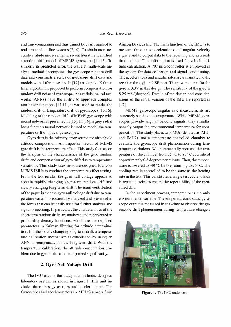
The IMU used in this study is an in-house designed

laboratory system, as shown in Figure 1. This unit in-

cludes three axes gyroscopes and accelerometers. The

Gyroscopes and accelerometers are MEMS sensors from

Analog Devices Inc. The main function of the IMU is to

measure three axes accelerations and angular velocity

signals and to output data to the receiving end in a real-

time manner. This information is used for vehicle atti-

tude calculation. A PIC microcontroller is employed in

the system for data collection and signal conditioning.

The accelerations and angular rates are transmitted to the

receiver through an USB port. The power source for the

gyro is 3.3V in this design. The sensitivity of the gyro is

8.25 mV/(deg/sec). Details of the design and consider-

ations of the initial version of the IMU are reported in

[17].

MEMS gyroscope angular rate measurements are

extremely sensitive to temperature. While MEMS gyro-

scopes provide angular velocity signals, they simulta-

neously output the environmental temperature for com-

pensation. This study places two IMUs (denoted as IMU1

and IMU2) into a temperature controlled chamber to

evaluate the gyroscope drift phenomenon during tem-

perature variations. We incrementally increase the tem-

perature of the chamber from 25 �C to 80 �C at a rate of

approximately 0.8 degrees per minute. Then, the temper-

ature is lowered to -40 �C before returning to 25 �C. The

cooling rate is controlled to be the same as the heating

rate in the test. This constitutes a single test cycle, which

is repeated twice to ensure the repeatability of the mea-

sured data.

In the experiment process, temperature is the only

environmental variable. The temperature and static gyro-

scope output is measured in real-time to observe the gy-

roscope drift phenomenon during temperature changes.

240 Jaw-Kuen Shiau et al.

Figure 1. The IMU under test.

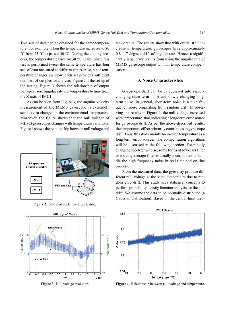
Two sets of data can be obtained for the same tempera-

ture. For example, when the temperature increases to 80

�C from 25 �C, it passes 30 �C. During the cooling pro-

cess, the temperature passes by 30 �C again. Since this

test is performed twice, the same temperature has four

sets of data measured at different times. Also, since tem-

perature changes are slow, each set provides sufficient

numbers of samples for analysis. Figure 2 is the set-up of

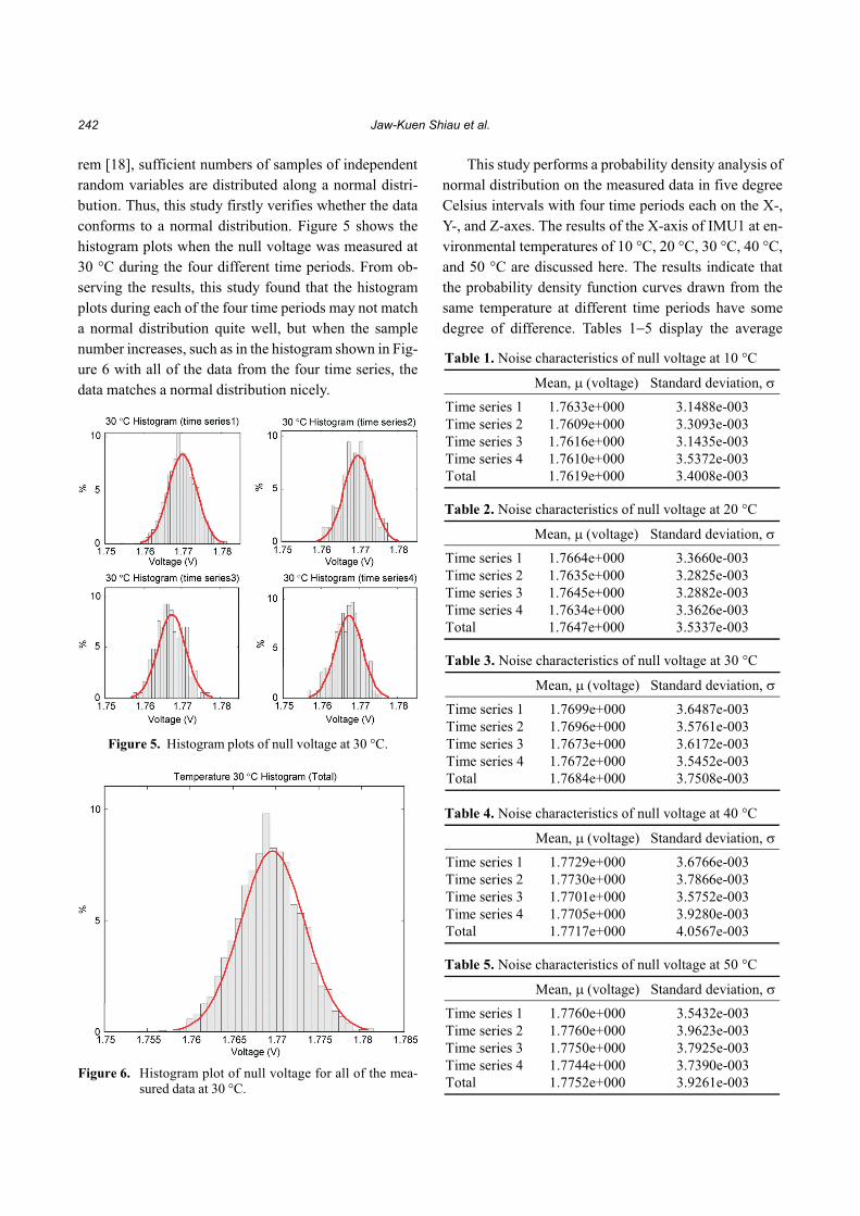
the testing. Figure 3 shows the relationship of output

voltage at zero angular rate and temperature to time from

the X-axis of IMU1.

As can be seen from Figure 3, the angular velocity

measurement of the MEMS gyroscope is extremely

sensitive to changes in the environmental temperature.

Moreover, the figure shows that the null voltage of

MEMS gyroscopes changes with temperature variations.

Figure 4 shows the relationship between null voltage and

temperature. The results show that with every 10 �C in-

crease in temperature, gyroscopes have approximately

0.8~1.7 deg/sec drift of angular rate. Hence, a signifi-

cantly large error results from using the angular rate of

MEMS gyroscope output without temperature compen-

sation.

3. Noise Characteristics

Gyroscope drift can be categorized into rapidly

changing short-term noise and slowly changing long-

term noise. In general, short-term noise is a high fre-

quency noise originating from random drift. In obser-

ving the results in Figure 4, the null voltage increased

with temperature, thus indicating a long-term error source

for gyroscope drift. As per the above-described results,

the temperature effect primarily contributes to gyroscope

drift. Thus, this study mainly focuses on temperature as a

long-term error source. The compensation algorithms

will be discussed in the following section. For rapidly

changing short-term noise, some forms of low-pass filter

or moving average filter is usually incorporated to han-

dle the high frequency noise in real-time and on-line

process.

From the measured data, the gyro may produce dif-

ferent null voltage at the same temperature due to ran-

dom gyro drift. This study uses statistical concepts to

perform probability density function analysis for the null

drift. We assume the data to be normally distributed (a

Gaussian distribution). Based on the central limit theo-

Noise Characteristics of MEMS Gyro’s Null Drift and Temperature Compensation 241

Figure 2. Set-up of the temperature testing.

Figure 3. Null voltage evolution. Figure 4. Relationship between null voltage and temperature.

rem [18], sufficient numbers of samples of independent

random variables are distributed along a normal distri-

bution. Thus, this study firstly verifies whether the data

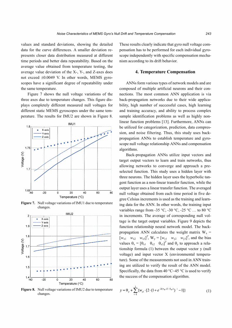
conforms to a normal distribution. Figure 5 shows the

histogram plots when the null voltage was measured at

30 �C during the four different time periods. From ob-

serving the results, this study found that the histogram

plots during each of the four time periods may not match

a normal distribution quite well, but when the sample

number increases, such as in the histogram shown in Fig-

ure 6 with all of the data from the four time series, the

data matches a normal distribution nicely.

This study performs a probability density analysis of

normal distribution on the measured data in five degree

Celsius intervals with four time periods each on the X-,

Y-, and Z-axes. The results of the X-axis of IMU1 at en-

vironmental temperatures of 10 �C, 20 �C, 30 �C, 40 �C,

and 50 �C are discussed here. The results indicate that

the probability density function curves drawn from the

same temperature at different time periods have some

degree of difference. Tables 1�5 display the average


Figure 5. Histogram plots of null voltage at 30 �C.

Figure 6. Histogram plot of null voltage for all of the mea-sured data at 30 �C.

Table 1. Noise characteristics of null voltage at 10 �C

Mean, � (voltage) Standard deviation, �

Time series 1 1.7633e+000 3.1488e-003

Time series 2 1.7609e+000 3.3093e-003

Time series 3 1.7616e+000 3.1435e-003

Time series 4 1.7610e+000 3.5372e-003

Total 1.7619e+000 3.4008e-003



Time series 1 1.7664e+000 3.3660e-003

Time series 2 1.7635e+000 3.2825e-003

Time series 3 1.7645e+000 3.2882e-003

Time series 4 1.7634e+000 3.3626e-003

Total 1.7647e+000 3.5337e-003



Time series 1 1.7699e+000 3.6487e-003

Time series 2 1.7696e+000 3.5761e-003

Time series 3 1.7673e+000 3.6172e-003

Time series 4 1.7672e+000 3.5452e-003

Total 1.7684e+000 3.7508e-003



Time series 1 1.7729e+000 3.6766e-003

Time series 2 1.7730e+000 3.7866e-003

Time series 3 1.7701e+000 3.5752e-003

Time series 4 1.7705e+000 3.9280e-003

Total 1.7717e+000 4.0567e-003



Time series 1 1.7760e+000 3.5432e-003

Time series 2 1.7760e+000 3.9623e-003

Time series 3 1.7750e+000 3.7925e-003

Time series 4 1.7744e+000 3.7390e-003

Total 1.7752e+000 3.9261e-003

values and standard deviations, showing the detailed

data for the curve differences. A smaller deviation re-

presents closer data distribution measured at different

time periods and better data repeatability. Based on the

average value obtained from temperature testing, the

average value deviation of the X-, Y-, and Z-axes does

not exceed �0.0049 V. In other words, MEMS gyro-

scopes have a significant degree of repeatability under

the same temperature.

Figure 7 shows the null voltage variations of the

three axes due to temperature changes. This figure dis-

plays completely different measured null voltages for

different static MEMS gyroscopes under the same tem-

perature. The results for IMU2 are shown in Figure 8.

These results clearly indicate that gyro null voltage com-

pensation has to be performed for each individual gyro-

scope independently with specific compensation mecha-

nism according to its drift behavior.

4. Temperature Compensation

ANNs form various types of network models and are

composed of multiple artificial neurons and their con-

nections. The most common ANN application is via

back-propagation networks due to their wide applica-

bility, high number of successful cases, high learning

and training accuracy, and ability to process complex

sample identification problems as well as highly non-

linear function problems [13]. Furthermore, ANNs can

be utilized for categorization, prediction, data compres-

sion, and noise filtering. Thus, this study uses back-

propagation ANNs to establish temperature and gyro-

scope null voltage relationship ANNs and compensation

algorithms.

Back-propagation ANNs utilize input vectors and

target output vectors to learn and train networks, thus

allowing networks to converge and approach a pre-

selected function. This study uses a hidden layer with

three neurons. The hidden layer uses the hyperbolic tan-

gent function as a non-linear transfer function, while the

output layer uses a linear transfer function. The averaged

null voltage obtained from each time period in five de-

gree Celsius increments is used as the training and learn-

ing data for the ANN. In other words, the training input

variables range from -35 �C, -30 �C, -25 �C … to 80 �C

in increments. The average of corresponding null vol-

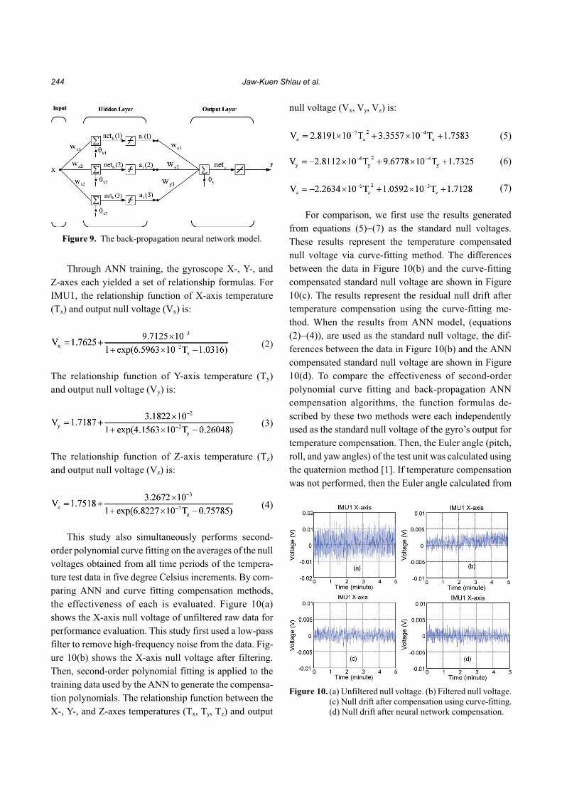
tage is the target output variables. Figure 9 depicts the

function relationship neural network model. The back-

propagation ANN calculates the weight matrix Wx =

[wx1 wx2 wx3]T, Wy = [wy1 wy2 wy3]

T, and the bias

values �x = [�x1 �x2 �x3]T and �y to approach a rela-

tionship formula (1) between the output vector y (null

voltage) and input vector X (environmental tempera-

ture). Some of the measurements not used in ANN train-

ing are utilized to verify the result of the ANN model.

Specifically, the data from 40 �C~45 �C is used to verify

the success of the compensation algorithm.

(1)


Figure 7. Null voltage variations of IMU1 due to temperaturechanges.

Figure 8. Null voltage variations of IMU2 due to temperaturechanges.

Through ANN training, the gyroscope X-, Y-, and

Z-axes each yielded a set of relationship formulas. For

IMU1, the relationship function of X-axis temperature

(Tx) and output null voltage (Vx) is:

(2)

The relationship function of Y-axis temperature (Ty)

and output null voltage (Vy) is:

(3)

The relationship function of Z-axis temperature (Tz)

and output null voltage (Vz) is:

(4)

This study also simultaneously performs second-

order polynomial curve fitting on the averages of the null

voltages obtained from all time periods of the tempera-

ture test data in five degree Celsius increments. By com-

paring ANN and curve fitting compensation methods,

the effectiveness of each is evaluated. Figure 10(a)

shows the X-axis null voltage of unfiltered raw data for

performance evaluation. This study first used a low-pass

filter to remove high-frequency noise from the data. Fig-

ure 10(b) shows the X-axis null voltage after filtering.

Then, second-order polynomial fitting is applied to the

training data used by the ANN to generate the compensa-

tion polynomials. The relationship function between the

X-, Y-, and Z-axes temperatures (Tx, Ty, Tz) and output

null voltage (Vx, Vy, Vz) is:

(5)

(6)

(7)

For comparison, we first use the results generated

from equations (5)�(7) as the standard null voltages.

These results represent the temperature compensated

null voltage via curve-fitting method. The differences

between the data in Figure 10(b) and the curve-fitting

compensated standard null voltage are shown in Figure

10(c). The results represent the residual null drift after

temperature compensation using the curve-fitting me-

thod. When the results from ANN model, (equations

(2)�(4)), are used as the standard null voltage, the dif-

ferences between the data in Figure 10(b) and the ANN

compensated standard null voltage are shown in Figure

10(d). To compare the effectiveness of second-order

polynomial curve fitting and back-propagation ANN

compensation algorithms, the function formulas de-

scribed by these two methods were each independently

used as the standard null voltage of the gyro’s output for

temperature compensation. Then, the Euler angle (pitch,

roll, and yaw angles) of the test unit was calculated using

the quaternion method [1]. If temperature compensation

was not performed, then the Euler angle calculated from


Figure 9. The back-propagation neural network model.

Figure 10. (a) Unfiltered null voltage. (b) Filtered null voltage.(c) Null drift after compensation using curve-fitting.(d) Null drift after neural network compensation.

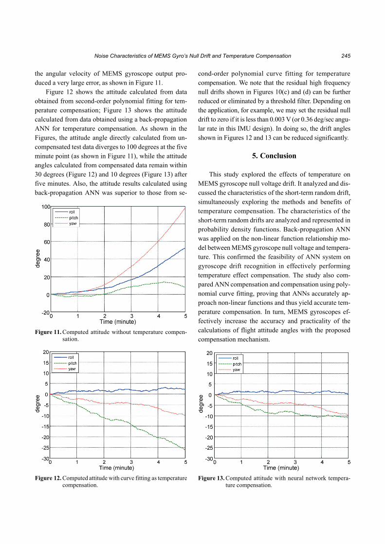
the angular velocity of MEMS gyroscope output pro-

duced a very large error, as shown in Figure 11.

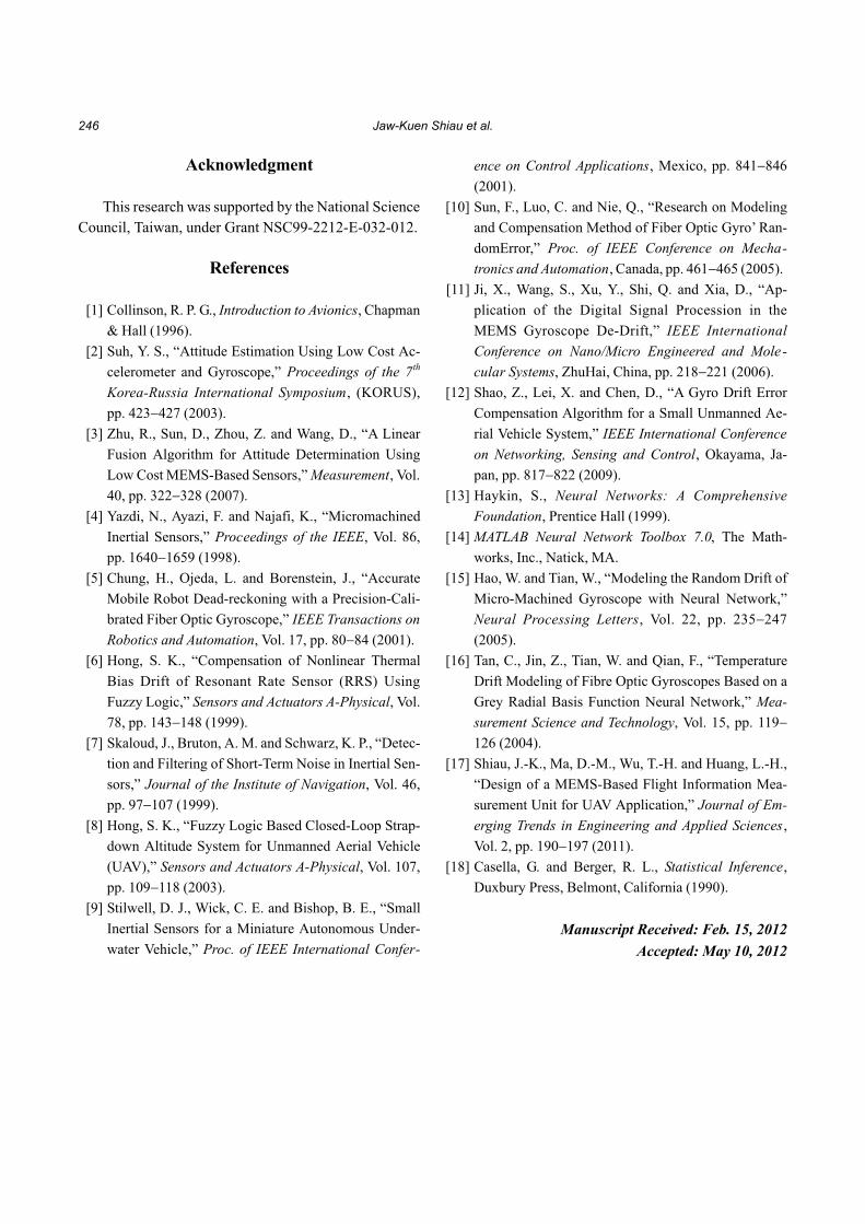
Figure 12 shows the attitude calculated from data

obtained from second-order polynomial fitting for tem-

perature compensation; Figure 13 shows the attitude

calculated from data obtained using a back-propagation

ANN for temperature compensation. As shown in the

Figures, the attitude angle directly calculated from un-

compensated test data diverges to 100 degrees at the five

minute point (as shown in Figure 11), while the attitude

angles calculated from compensated data remain within

30 degrees (Figure 12) and 10 degrees (Figure 13) after

five minutes. Also, the attitude results calculated using

back-propagation ANN was superior to those from se-

cond-order polynomial curve fitting for temperature

compensation. We note that the residual high frequency

null drifts shown in Figures 10(c) and (d) can be further

reduced or eliminated by a threshold filter. Depending on

the application, for example, we may set the residual null

drift to zero if it is less than 0.003 V (or 0.36 deg/sec angu-

lar rate in this IMU design). In doing so, the drift angles

shown in Figures 12 and 13 can be reduced significantly.

5. Conclusion

This study explored the effects of temperature on

MEMS gyroscope null voltage drift. It analyzed and dis-

cussed the characteristics of the short-term random drift,

simultaneously exploring the methods and benefits of

temperature compensation. The characteristics of the

short-term random drifts are analyzed and represented in

probability density functions. Back-propagation ANN

was applied on the non-linear function relationship mo-

del between MEMS gyroscope null voltage and tempera-

ture. This confirmed the feasibility of ANN system on

gyroscope drift recognition in effectively performing

temperature effect compensation. The study also com-

pared ANN compensation and compensation using poly-

nomial curve fitting, proving that ANNs accurately ap-

proach non-linear functions and thus yield accurate tem-

perature compensation. In turn, MEMS gyroscopes ef-

fectively increase the accuracy and practicality of the

calculations of flight attitude angles with the proposed

compensation mechanism.


Figure 11. Computed attitude without temperature compen-sation.

Figure 12. Computed attitude with curve fitting as temperaturecompensation.

Figure 13. Computed attitude with neural network tempera-ture compensation.

Acknowledgment

This research was supported by the National Science

Council, Taiwan, under Grant NSC99-2212-E-032-012.

References

[1] Collinson, R. P. G., Introduction to Avionics, Chapman

& Hall (1996).

[2] Suh, Y. S., “Attitude Estimation Using Low Cost Ac-

celerometer and Gyroscope,” Proceedings of the 7th

Korea-Russia International Symposium, (KORUS),

pp. 423�427 (2003).

[3] Zhu, R., Sun, D., Zhou, Z. and Wang, D., “A Linear

Fusion Algorithm for Attitude Determination Using

Low Cost MEMS-Based Sensors,” Measurement, Vol.

40, pp. 322�328 (2007).

[4] Yazdi, N., Ayazi, F. and Najafi, K., “Micromachined

Inertial Sensors,” Proceedings of the IEEE, Vol. 86,

pp. 1640�1659 (1998).

[5] Chung, H., Ojeda, L. and Borenstein, J., “Accurate

Mobile Robot Dead-reckoning with a Precision-Cali-

brated Fiber Optic Gyroscope,” IEEE Transactions on

Robotics and Automation, Vol. 17, pp. 80�84 (2001).

[6] Hong, S. K., “Compensation of Nonlinear Thermal

Bias Drift of Resonant Rate Sensor (RRS) Using

Fuzzy Logic,” Sensors and Actuators A-Physical, Vol.

78, pp. 143�148 (1999).

[7] Skaloud, J., Bruton, A. M. and Schwarz, K. P., “Detec-

tion and Filtering of Short-Term Noise in Inertial Sen-

sors,” Journal of the Institute of Navigation, Vol. 46,

pp. 97�107 (1999).

[8] Hong, S. K., “Fuzzy Logic Based Closed-Loop Strap-

down Altitude System for Unmanned Aerial Vehicle

(UAV),” Sensors and Actuators A-Physical, Vol. 107,

pp. 109�118 (2003).

[9] Stilwell, D. J., Wick, C. E. and Bishop, B. E., “Small

Inertial Sensors for a Miniature Autonomous Under-

water Vehicle,” Proc. of IEEE International Confer-

ence on Control Applications, Mexico, pp. 841�846

(2001).

[10] Sun, F., Luo, C. and Nie, Q., “Research on Modeling

and Compensation Method of Fiber Optic Gyro’ Ran-

domError,” Proc. of IEEE Conference on Mecha-

tronics and Automation, Canada, pp. 461�465 (2005).

[11] Ji, X., Wang, S., Xu, Y., Shi, Q. and Xia, D., “Ap-

plication of the Digital Signal Procession in the

MEMS Gyroscope De-Drift,” IEEE International

Conference on Nano/Micro Engineered and Mole-

cular Systems, ZhuHai, China, pp. 218�221 (2006).

[12] Shao, Z., Lei, X. and Chen, D., “A Gyro Drift Error

Compensation Algorithm for a Small Unmanned Ae-

rial Vehicle System,” IEEE International Conference

on Networking, Sensing and Control, Okayama, Ja-

pan, pp. 817�822 (2009).

[13] Haykin, S., Neural Networks: A Comprehensive

Foundation, Prentice Hall (1999).

[14] MATLAB Neural Network Toolbox 7.0, The Math-

works, Inc., Natick, MA.

[15] Hao, W. and Tian, W., “Modeling the Random Drift of

Micro-Machined Gyroscope with Neural Network,”

Neural Processing Letters, Vol. 22, pp. 235�247

(2005).

[16] Tan, C., Jin, Z., Tian, W. and Qian, F., “Temperature

Drift Modeling of Fibre Optic Gyroscopes Based on a

Grey Radial Basis Function Neural Network,” Mea-

surement Science and Technology, Vol. 15, pp. 119�

126 (2004).

[17] Shiau, J.-K., Ma, D.-M., Wu, T.-H. and Huang, L.-H.,

“Design of a MEMS-Based Flight Information Mea-

surement Unit for UAV Application,” Journal of Em-

erging Trends in Engineering and Applied Sciences,

Vol. 2, pp. 190�197 (2011).

[18] Casella, G. and Berger, R. L., Statistical Inference,

Duxbury Press, Belmont, California (1990).

Manuscript Received: Feb. 15, 2012

Accepted: May 10, 2012


Documents

Noise Characteristics of MEMS Gyro's Null Drift and Temperature Compensation