Noise Mapping in an Urban Environment: Comparing GIS-based

122 Full Paper

Journal of Digital Landscape Architecture, 5-2020, pp. 122-129. © Wichmann Verlag, VDE VERLAG GMBH ꞏ Berlin ꞏ Offenbach. ISBN 978-3-87907-690-1, ISSN 2367-4253, e-ISSN 2511-624X, doi:10.14627/537690013. This article is an open access article distributed under the terms and conditions of the Creative Commons Attribution license (http://creativecommons.org/licenses/by-nd/4.0/).

Noise Mapping in an Urban Environment: Comparing GIS-based Spatial Modelling and Parametric Approaches

Siqing Chen1, Zhizhen Wang2

1University of Melbourne, Melbourne/Australia ꞏ [email protected] 2University of Melbourne, Melbourne/Australia

Abstract: We conduct noise mapping for an inner-suburb precinct adjacent to Melbourne CBD using GIS geostatistical interpolation and parametric (Rhino and Grasshopper) approaches, based on traffic noise data collected using field measurement. We then compare the spatial and temporal patterns of noise dynamics based on measured noise data and modelled noise level outputs. Preliminary findings shed lights on understanding traffic flows and noise level, noise attenuation through landform and tree planting, etc. We discuss the effectiveness and compatibility of the two modelling approaches, and potential applications of the outcomes of this study in informing landscape planning and design to mit-igate noise pollution in the urban environment.

Keywords: Noise mapping, spatial modelling, parametric simulation

1 Introduction

Noise pollution is increasingly considered a critical threat to mental and physical health for urban populations worldwide (ROSENBERG 2016). Noise nuisance has been a major environ-mental complaint in urban residential areas as it impacts many areas with high population density and affects the inhabitants in their daily life. In some cities, resident petitions to re-duce noise pollution are more common than those for air pollution (DAS et al. 2019). WHO recommends that night sound levels outside of the living spaces should not exceed 45 dB, so that people may sleep with bedroom windows open (WHO 1999). In Australia, Noise is reg-ulated by the Environment Protection Act 1997 and the Environment Protection Regulation 2005, which aim to protect people from undue noise while facilitating business and social activities as well as state and municipal legislation and standards. In typical residential areas in ACT, noise can’t exceed 45 dB between 7am-10pm on weekdays (8am-10pm on Sunday and public holidays) or 35 dB between 10pm-7am on weekdays (10pm-8am on Sunday and public holidays), while the consequent levels of noise for business-related area should are 60 and 50 dB respectively (accesscanberra.act.gov.au).

Noise mapping is one of the best ways of understanding environmental noise. A noise map can be used to quantify main sources of noise; facilitate the development of policies for con-trolling noise and enforcing the control of noise and monitor noise reduction schemes and their effectiveness during the enforcement processes (TSAI et al. 2009). Since the musician R. M. Schafer raised the concern about noise pollution in the 1960s (SCHAFER 1969), many studies have been carried out for noise mapping (DAS et al. 2019, MEHDI et al. 2011, TSAI et al. 2009, WANG & KANG 2011) and recently soundscape design (LIU et al. 2019, PÉREZ-MARTÍNEZ et al. 2018). Both GIS-based spatial modelling and parametric approaches (e. g. Rhino, Grasshopper and other plugins) have been used for noise mapping. However, GIS-based approaches are more suitable for noise mapping in larger outdoor spaces (DAS et al.

S. Chen, Z. Wang: Noise Mapping in an Urban Environment 123

2019, TSAI et al. 2009) while the parametric approaches are used primarily for acoustic sim-ulation in architecture design workflows (PETERS 2015). There are very few studies on com-paring the two approaches’ strength and weakness in noise mapping in an urban environment.

Among all sources of noise, traffic noise is of the top concern according to a community noise survey in Victoria (STRAHAN RESEARCH 2007). In this study, we compare effectiveness and compatibility of the GIS-based spatial modelling and parametric approaches for noise mapping for an inner-city precinct suffering high traffic noise exposure from road, tram and train traffic in Melbourne, Australia, where increasing traffic density, growing population, infill development, construction and renovation works are causing increasing noise pollution and annoyance.

2 Data and Methods

2.1 Study Area

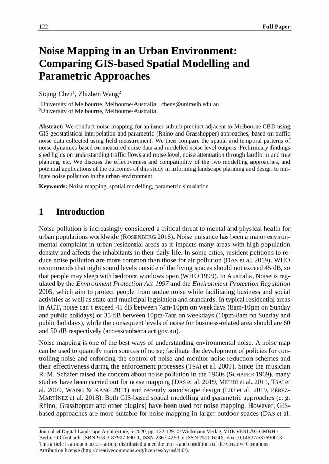
We use the public green space near Flemington Rd and the exterior area of the Royal Chil-dren’s Hospital (RCH) on the south side to measure the noise level and soundscape potential in the inner-suburb precinct. This triangle area is surrounded by Flemington Rd, Elliot Ave and Route 58 Tram Track (Fig. 1). The elevation is slightly higher in the north part of the site. There are a large numbers of tree groves, shrubs, maintained lawn, and other vegetation communities on this site. Walking tracks and bike paths on the site enable daily visits and other civic uses of the site.

Fig. 1: The study area: an inner suburb precinct adjacent to Melbourne CBD

124 Journal of Digital Landscape Architecture ꞏ 5-2020

Flemington Rd is one of the heaviest traffic thoroughfares in Melbourne, it serves the north-ern and western suburbs to quickly link to the Melbourne CBD. This 60-metre wide major road includes by 8 car lanes, three tram tracks (route 57, 58, 59), two bike lanes and two pedestrian paths. It connects CityLink (toll expressway) to Melbourne Airport and other ma-jor arterial roads to Melbourne CBD. The heavy traffic and traffic noise on this road have been exacerbated by the addition of Royal Children’s Hospital (largest specialist pediat-ric hospital in Victoria) on the southeast corner of the site. The location and its context make it an ideal site for this study.

2.2 Noise Data Collection

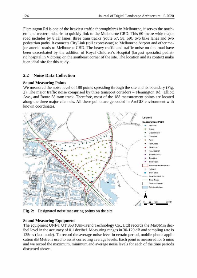
Sound Measuring Points We measured the noise level of 188 points spreading through the site and its boundary (Fig. 2). The major traffic noise comprised by three transport corridors – Flemington Rd., Elliott Ave., and Route 58 tram track. Therefore, most of the 188 measurement points are located along the three major channels. All these points are geocoded in ArcGIS environment with known coordinates.

Fig. 2: Designated noise measuring points on the site

Sound Measuring Equipment The equipment UNI-T UT 353 (Uni-Trend Technology Co., Ltd) records the Max/Min dec-ibel level in the accuracy of 0.1 decibel. Measuring ranges in 30-120 dB and sampling rate is 125ms (fast mode). To record the average noise level in certain period, mobile phone appli-cation dB Metre is used to assist correcting average levels. Each point is measured for 5 mins and we record the maximum, minimum and average noise levels for each of the time periods discussed above.


Nosie Measuring Periods Like many inner suburb sites, the traffic through the study area is polarised on weekday morn-ing and night, due to track to and from the adjacent CBD as the largest employment centre in Melbourne. Therefore, weekday measurements are split into morning, noon, and evening to capture the effects of daily traffic patterns on noise level. Maximum, average and minimum sound level were recorded for each of these times and weekend.

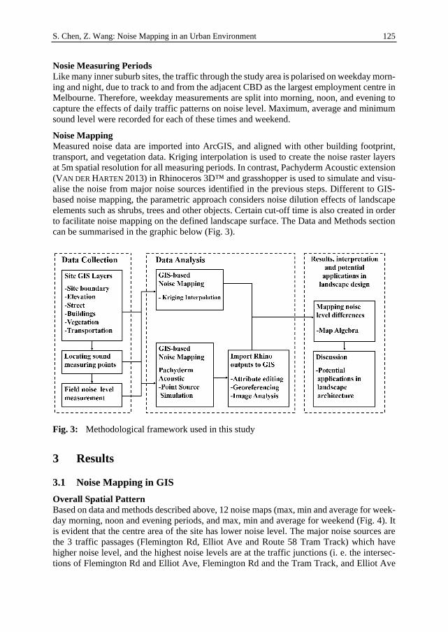
Noise Mapping Measured noise data are imported into ArcGIS, and aligned with other building footprint, transport, and vegetation data. Kriging interpolation is used to create the noise raster layers at 5m spatial resolution for all measuring periods. In contrast, Pachyderm Acoustic extension (VAN DER HARTEN 2013) in Rhinoceros 3D™ and grasshopper is used to simulate and visu-alise the noise from major noise sources identified in the previous steps. Different to GIS-based noise mapping, the parametric approach considers noise dilution effects of landscape elements such as shrubs, trees and other objects. Certain cut-off time is also created in order to facilitate noise mapping on the defined landscape surface. The Data and Methods section can be summarised in the graphic below (Fig. 3).

Fig. 3: Methodological framework used in this study

3 Results

3.1 Noise Mapping in GIS

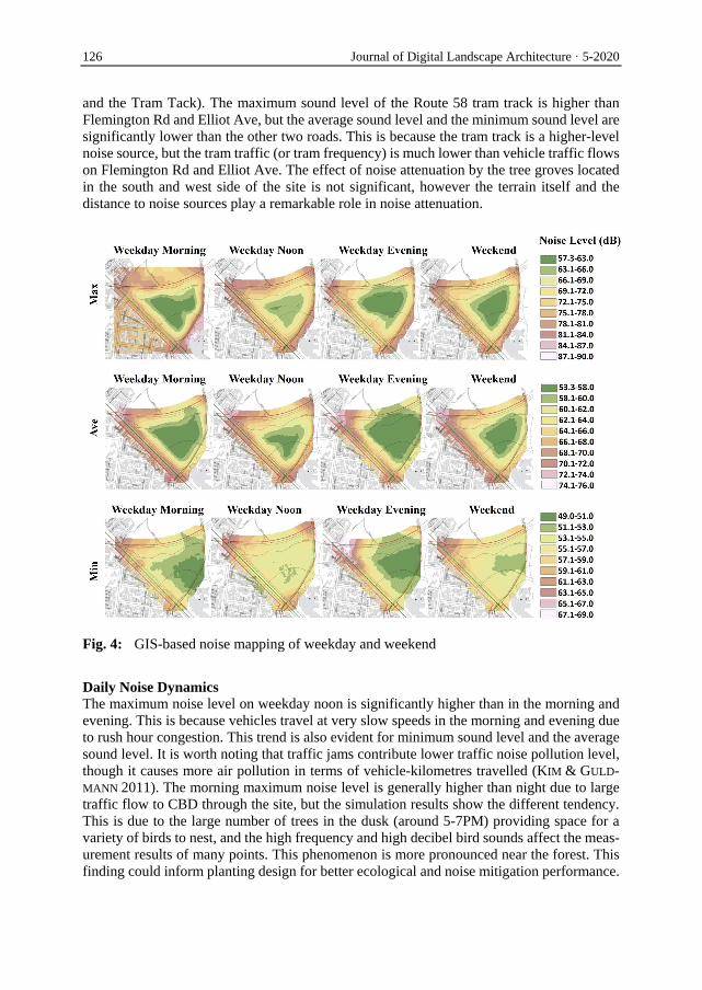
Overall Spatial Pattern Based on data and methods described above, 12 noise maps (max, min and average for week-day morning, noon and evening periods, and max, min and average for weekend (Fig. 4). It is evident that the centre area of the site has lower noise level. The major noise sources are the 3 traffic passages (Flemington Rd, Elliot Ave and Route 58 Tram Track) which have higher noise level, and the highest noise levels are at the traffic junctions (i. e. the intersec-tions of Flemington Rd and Elliot Ave, Flemington Rd and the Tram Track, and Elliot Ave


and the Tram Tack). The maximum sound level of the Route 58 tram track is higher than Flemington Rd and Elliot Ave, but the average sound level and the minimum sound level are significantly lower than the other two roads. This is because the tram track is a higher-level noise source, but the tram traffic (or tram frequency) is much lower than vehicle traffic flows on Flemington Rd and Elliot Ave. The effect of noise attenuation by the tree groves located in the south and west side of the site is not significant, however the terrain itself and the distance to noise sources play a remarkable role in noise attenuation.

Fig. 4: GIS-based noise mapping of weekday and weekend

Daily Noise Dynamics The maximum noise level on weekday noon is significantly higher than in the morning and evening. This is because vehicles travel at very slow speeds in the morning and evening due to rush hour congestion. This trend is also evident for minimum sound level and the average sound level. It is worth noting that traffic jams contribute lower traffic noise pollution level, though it causes more air pollution in terms of vehicle-kilometres travelled (KIM & GULD-MANN 2011). The morning maximum noise level is generally higher than night due to large traffic flow to CBD through the site, but the simulation results show the different tendency. This is due to the large number of trees in the dusk (around 5-7PM) providing space for a variety of birds to nest, and the high frequency and high decibel bird sounds affect the meas-urement results of many points. This phenomenon is more pronounced near the forest. This finding could inform planting design for better ecological and noise mitigation performance.


Weekly Noise Dynamics The maximum and average noise level on weekend display a more balanced and even ten-dency than on weekday, and there is no obvious tidal traffic on the three main traffic routes. However, the site on weekend have a higher minimum noise level. This is due to more activ-ities such as football, tennis and cycling, and the weekend traffic speed is also higher than the working day. Large noise ranges are evident based on the noise mapping results, which confirm the field measurement (Table 1). The maximum measured noise level is 90.1 dB on weekend on a pedestrian track (not due to traffic). The modelled maximum noise levels (88.4 dB for GIS-based interpolation and 84.2 for Rhino based simulation) are slightly lower than the measured noise level. However, these levels are far above the standards stipulated by governmental law, indicating that urgent actions to mitigate the noise pollution are necessary.

Table 1: Noise level on different time of weekday and weekend (average of 188 points)

Time

Noise Level (dB)_

Measured Modelled (GIS) Modelled (Rhino)

Max Min Ave Max Min Ave Max Min Ave

Weekday morning 86.8 46.0 64.7 88.4 64.4 74.3 82.9 51.4 66.3

Weekday noon 88.0 47.7 65.3 84.6 65.1 73 84.2 56.5 68.4

Weekday evening 89.2 46.5 63.4 86.1 68.6 75.1 80.0 50.8 64.1

Weekend 90.1 50.4 65.2 85.9 51.9 73.8 83.7 53.9 66.6

3.2 Sound Simulation Using Parametric Approaches

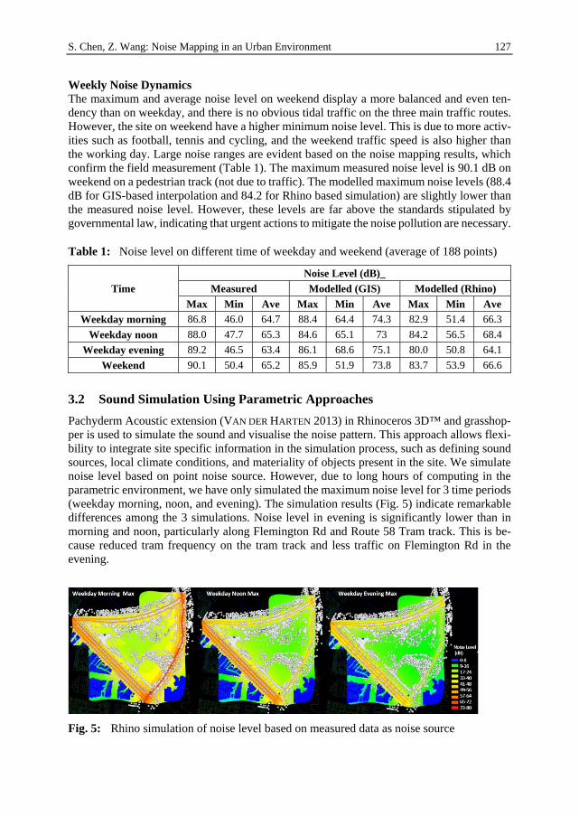
Pachyderm Acoustic extension (VAN DER HARTEN 2013) in Rhinoceros 3D™ and grasshop-per is used to simulate the sound and visualise the noise pattern. This approach allows flexi-bility to integrate site specific information in the simulation process, such as defining sound sources, local climate conditions, and materiality of objects present in the site. We simulate noise level based on point noise source. However, due to long hours of computing in the parametric environment, we have only simulated the maximum noise level for 3 time periods (weekday morning, noon, and evening). The simulation results (Fig. 5) indicate remarkable differences among the 3 simulations. Noise level in evening is significantly lower than in morning and noon, particularly along Flemington Rd and Route 58 Tram track. This is be-cause reduced tram frequency on the tram track and less traffic on Flemington Rd in the evening.

Fig. 5: Rhino simulation of noise level based on measured data as noise source


3.3 Differences between GIS- and Rhino-based Simulation Results

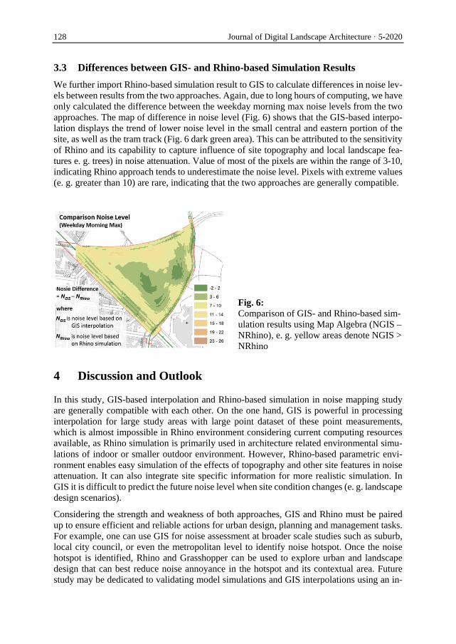
We further import Rhino-based simulation result to GIS to calculate differences in noise lev-els between results from the two approaches. Again, due to long hours of computing, we have only calculated the difference between the weekday morning max noise levels from the two approaches. The map of difference in noise level (Fig. 6) shows that the GIS-based interpo-lation displays the trend of lower noise level in the small central and eastern portion of the site, as well as the tram track (Fig. 6 dark green area). This can be attributed to the sensitivity of Rhino and its capability to capture influence of site topography and local landscape fea-tures e. g. trees) in noise attenuation. Value of most of the pixels are within the range of 3-10, indicating Rhino approach tends to underestimate the noise level. Pixels with extreme values (e. g. greater than 10) are rare, indicating that the two approaches are generally compatible.

Fig. 6: Comparison of GIS- and Rhino-based sim-ulation results using Map Algebra (NGIS – NRhino), e. g. yellow areas denote NGIS > NRhino

4 Discussion and Outlook

In this study, GIS-based interpolation and Rhino-based simulation in noise mapping study are generally compatible with each other. On the one hand, GIS is powerful in processing interpolation for large study areas with large point dataset of these point measurements, which is almost impossible in Rhino environment considering current computing resources available, as Rhino simulation is primarily used in architecture related environmental simu-lations of indoor or smaller outdoor environment. However, Rhino-based parametric envi-ronment enables easy simulation of the effects of topography and other site features in noise attenuation. It can also integrate site specific information for more realistic simulation. In GIS it is difficult to predict the future noise level when site condition changes (e. g. landscape design scenarios).

Considering the strength and weakness of both approaches, GIS and Rhino must be paired up to ensure efficient and reliable actions for urban design, planning and management tasks. For example, one can use GIS for noise assessment at broader scale studies such as suburb, local city council, or even the metropolitan level to identify noise hotspot. Once the noise hotspot is identified, Rhino and Grasshopper can be used to explore urban and landscape design that can best reduce noise annoyance in the hotspot and its contextual area. Future study may be dedicated to validating model simulations and GIS interpolations using an in-


dependent in-situ noise measurement dataset, such that the discrepancies in noise outputs based on the two approaches may be better understood. This study is one of the first attempts to explore the potential of comparing and pairing traditional GIS interpolation with paramet-ric approaches for noise mapping in a relatively large site. Despite its limitations, this study can still provide useful reference for pairing the two approaches for improved design out-comes in various relevant fields such as planting design in residential areas or public space for better soundscape outcomes.

References

DAS, P., TALUKDAR, S., ZIAUL, S., DAS, S. & PAL, S. (2019), Noise mapping and assessing vulnerability in meso level urban environment of Eastern India. Sustainable Cities and Society, 46, 101416. doi:10.1016/j.scs.2019.01.001.

KIM, Y. & GULDMANN, J.-M. (2011), Impact of traffic flows and wind directions on air pol-lution concentrations in Seoul, Korea. Atmospheric Environment, 45 (16), 2803-2810. doi:10.1016/j.atmosenv.2011.02.050.

LIU, J., WANG, Y., ZIMMER, C., KANG, J. & YU, T. (2019), Factors associated with soundscape experiences in urban green spaces: A case study in Rostock, Germany. Urban Forestry & Urban Greening, 37, 135-146. doi:10.1016/j.ufug.2017.11.003.

MEHDI, M. R., KIM, M., SEONG, J. C. & ARSALAN, M. H. (2011), Spatio-temporal patterns of road traffic noise pollution in Karachi, Pakistan. Environment International, 37 (1), 97-104. doi:10.1016/J.ENVINT.2010.08.003.

PÉREZ-MARTÍNEZ, G., TORIJA, A. J. & RUIZ, D. P. (2018), Soundscape assessment of a mon-umental place: A methodology based on the perception of dominant sounds. Landscape and Urban Planning, 169, 12-21. doi:10.1016/j.landurbplan.2017.07.022.

PETERS, B. (2015), Integrating acoustic simulation in architectural design workflows: the FabPod meeting room prototype. Simulation, 91 (9), 787-808. doi:10.1177/0037549715603480.

ROSENBERG, B. C. (2016), Shhh! Noisy cities, anti-noise groups and neoliberal citizenship. Journal of Sociology, 52, 190-203. doi:10.1177/1440783313507493.

SCHAFER, R. M. (1994), Our sonic environment and the soundscape: The tuning of the world. Destiny Books, Rochester, Vermont.

STRAHAN RESEARCH (2007), Report to EPA Victoria on community response to environmen-tal noise. Melbourne Victoria.

TSAI, K. T., LIN, M. D. & CHEN, Y. H. (2009), Noise mapping in urban environments: A Tai-wan study. Applied Acoustics, 70 (7), 964-972. doi:10.1016/j.apacoust.2008.11.001.

VAN DER HARTEN, A. (2013), Pachyderm Acoustical Simulation: Towards Open-Source Sound Analysis. Architectural Design, 83 (2), 138-139. doi:10.1002/ad.1570.

WANG, B. & KANG, J. (2011), Effects of urban morphology on the traffic noise distribution through noise mapping: A comparative study between UK and China. Applied Acoustics, 72 (8), 556-568. doi:10.1016/j.apacoust.2011.01.011.

WHO (1999), Guidelines for Community Noise. https://www.who.int/docstore/peh/noise/Comnoise-1.pdf (28.02.2020).

Documents

Noise Mapping in an Urban Environment: Comparing GIS-based