Embed Size (px)
Citation preview

Non-linear MagnetohydrodynamicInstabilities In Advanced Tokamak
Plasmas
Rachel McAdams
Doctor of Philosophy
University Of York
Physics
September 2014
Abstract
Dwindling fossil fuel resources, and the undesirable environmental effects associated with
their use in power generation, are a powerful impetus in the search for clean, reliable and
inexpensive methods of generating electricity. Fusion is a process wherein light nuclei are
able to fuse together, releasing large amounts of energy. Magnetic Confinement Fusion
is one concept for harnessing this energy for electricity production. The tokamak reactor
confines the plasma in a toroidal configuration using strong magnetic fields to minimise
particle and heat losses from the plasma. However, this plasma can become unstable,
resulting in loss of plasma confinement, or plasma disruption.
In particular, the instability known as the Resistive Wall Mode (RWM) is of concern for
operating scenarios which are designed to optimise the fusion process, yet lie close to
mode stability boundaries. The RWM is a global instability, which can cause plasma dis-
ruption. The mode is so named because it is only present when the plasma is surrounded
by a resistive wall. Theoretical and experimental studies have found that plasma rota-
tion is able to stabilise the RWM; yet in projected operating scenarios for ITER, the
plasma rotation will fall below the levels found in present tokamaks. Understanding the
stability of the RWM in ’advanced’ scenarios is crucial, and requires non-linear physics
to incorporate all the characteristics of the mode.
In this thesis, the Introduction describes the need for the development of fusion energy,
and why the RWM is an important consideration in planning for future experimental
programmes. The Literature Review summarises the current state of knowledge sur-
rounding the RWM and its stability in tokamak plasmas. In Chapter 3, an analytic
study of the RWM is presented. In this study, the mode is coupled to a different mode,
known as the Neoclassical Tearing Mode. A system of non-linear equations describing
the coupling of the modes in a rotating plasma is derived. In Chapter 4, these equations
are solved for limiting solutions, and solved numerically, to show how the RWM may
be responsible for an observed phenomenon called the triggerless NTM. Chapter 5 and
Chapter 6 focus on simulations of RWMs. Chapter 5 describes the implementation of a
resistive wall in the non-linear MHD code JOREK, carried out by M. Holzl. This imple-
mentation is benchmarked successfully against a linear analytic formula for the RWM
growth rate. In Chapter 6, initial simulations using the resistive wall in JOREK are
carried out. These simulations are carried out in ITER geometry, with the resistive wall
modelling the ITER first wall. Chapter 7 summarises the conclusions of the research
chapters and lays out future work which could be undertaken in both analytic modelling
and simulations.
Contents
Abstract i
Contents ii
List of Figures v
Acknowledgements vii
Declaration of Authorship viii
1 Introduction 1
1.1 Energy crisis and projections . . . . . . . . . . . . . . . . . . . . . . . . . 1
1.2 Fusion energy . . . . . . . . . . . . . . . . . . . . . . . . . . . . . . . . . . 3
1.2.1 The Fusion Reaction . . . . . . . . . . . . . . . . . . . . . . . . . . 3
1.2.1.1 Plasma Confinement . . . . . . . . . . . . . . . . . . . . . 5
1.3 Magnetic Confinement Fusion . . . . . . . . . . . . . . . . . . . . . . . . . 6
1.3.1 Flux Surfaces . . . . . . . . . . . . . . . . . . . . . . . . . . . . . . 6
1.4 Magnetohydrodynamics In Fusion Plasmas . . . . . . . . . . . . . . . . . 10
1.4.1 MHD Equations . . . . . . . . . . . . . . . . . . . . . . . . . . . . 10
1.4.2 MHD Instability . . . . . . . . . . . . . . . . . . . . . . . . . . . . 12
1.5 ITER . . . . . . . . . . . . . . . . . . . . . . . . . . . . . . . . . . . . . . 13
1.5.1 ITER Advanced Scenarios . . . . . . . . . . . . . . . . . . . . . . . 14
1.6 Scope Of The Thesis . . . . . . . . . . . . . . . . . . . . . . . . . . . . . . 18
2 Literature Review 20
2.1 Resistive Wall Modes In Tokamak Plasmas . . . . . . . . . . . . . . . . . 20
2.1.1 Resistive Walls . . . . . . . . . . . . . . . . . . . . . . . . . . . . . 20
2.2 RWM Dispersion Relation . . . . . . . . . . . . . . . . . . . . . . . . . . . 22
2.3 Experimental Resistive Wall Modes . . . . . . . . . . . . . . . . . . . . . . 23
2.3.1 Resistive Wall Modes And Plasma Rotation . . . . . . . . . . . . . 24
2.4 Resistive Wall Modes And Nonlinear Effects . . . . . . . . . . . . . . . . . 25
2.4.1 Plasma Rotation . . . . . . . . . . . . . . . . . . . . . . . . . . . . 25
2.4.2 Theoretical RWM Stabilisation Models . . . . . . . . . . . . . . . . 25
2.4.3 Torque Balance In A Tokamak . . . . . . . . . . . . . . . . . . . . 28
2.4.4 Rotation Threshold Experiments . . . . . . . . . . . . . . . . . . . 28
2.4.5 Torque Balance Models For The RWM . . . . . . . . . . . . . . . . 31
ii

Contents iii
2.4.6 Other Effects On Resistive Wall Modes . . . . . . . . . . . . . . . 32
2.5 RWM Control In ITER . . . . . . . . . . . . . . . . . . . . . . . . . . . . 33
3 Neoclassical Tearing Modes and Coupling to Resistive Wall Modes inRotating Plasmas 37
3.1 Theory Of Neoclassical Tearing Modes . . . . . . . . . . . . . . . . . . . . 37
3.1.1 Classical Tearing Modes . . . . . . . . . . . . . . . . . . . . . . . . 38
3.1.2 Neoclassical Effects On Tearing Mode Theory . . . . . . . . . . . . 39
3.2 Triggerless NTMs . . . . . . . . . . . . . . . . . . . . . . . . . . . . . . . . 42
3.3 Analytic Coupling Of Resistive Wall Mode To Neoclassical Tearing Mode 43
3.3.1 Evaluating Discontinuities Across Wall And Layer . . . . . . . . . 43
3.3.2 NTM Evolution . . . . . . . . . . . . . . . . . . . . . . . . . . . . . 46
3.4 Toroidal Torque Balance . . . . . . . . . . . . . . . . . . . . . . . . . . . . 49
3.5 Summary Of Results . . . . . . . . . . . . . . . . . . . . . . . . . . . . . . 50
4 Solutions For Coupled NTM-RWM In A Rotating Plasma 52
4.1 No Wall Solution . . . . . . . . . . . . . . . . . . . . . . . . . . . . . . . . 53
4.2 Limiting Solution For Small Islands . . . . . . . . . . . . . . . . . . . . . . 53
4.3 Numerical Solutions To Non-linear System . . . . . . . . . . . . . . . . . . 56
4.3.1 Dependence on β . . . . . . . . . . . . . . . . . . . . . . . . . . . . 58
4.3.2 Dependence on Ω0 . . . . . . . . . . . . . . . . . . . . . . . . . . . 60
4.3.3 Equilibrium Parameters . . . . . . . . . . . . . . . . . . . . . . . . 60
4.4 Summary of conclusions . . . . . . . . . . . . . . . . . . . . . . . . . . . . 62
4.4.1 Experimental Observations . . . . . . . . . . . . . . . . . . . . . . 62
4.4.2 Contrasting Interpretations Of Triggerless NTMs . . . . . . . . . . 66
4.5 Summary Of Results . . . . . . . . . . . . . . . . . . . . . . . . . . . . . . 67
5 Benchmarking Resistive Walls in JOREK 68
5.1 Nonlinear MHD Simulations With JOREK . . . . . . . . . . . . . . . . . 68
5.1.1 JOREK Equilibrium . . . . . . . . . . . . . . . . . . . . . . . . . . 68
5.1.2 Reduced MHD Equations . . . . . . . . . . . . . . . . . . . . . . . 69
5.2 Coupling JOREK And STARWALL . . . . . . . . . . . . . . . . . . . . . 70
5.2.1 STARWALL . . . . . . . . . . . . . . . . . . . . . . . . . . . . . . 71
5.2.2 Boundary Conditions . . . . . . . . . . . . . . . . . . . . . . . . . 71
5.2.3 Implementing The Boundary Integral . . . . . . . . . . . . . . . . 71
5.3 Benchmarking JOREK-STARWALL . . . . . . . . . . . . . . . . . . . . . 74
5.3.1 Linear Analysis Of RWM . . . . . . . . . . . . . . . . . . . . . . . 74
5.3.2 JOREK Equilibrium . . . . . . . . . . . . . . . . . . . . . . . . . . 77
5.4 Benchmarking Results . . . . . . . . . . . . . . . . . . . . . . . . . . . . . 78
5.4.1 Resistive Wall Benchmarking . . . . . . . . . . . . . . . . . . . . . 80
5.5 Summary Of Results . . . . . . . . . . . . . . . . . . . . . . . . . . . . . . 83
6 ITER simulations with JOREK and realistic wall 84
6.1 ITER Equilibrium . . . . . . . . . . . . . . . . . . . . . . . . . . . . . . . 84
6.1.1 Reducing The Edge Current . . . . . . . . . . . . . . . . . . . . . . 84
6.2 Features Of The Unstable Mode . . . . . . . . . . . . . . . . . . . . . . . 88
6.2.1 Plasma Resistivity Scan . . . . . . . . . . . . . . . . . . . . . . . . 90
6.2.2 Wall Resistivity Scan . . . . . . . . . . . . . . . . . . . . . . . . . . 93

Contents iv
6.2.3 βN Scan . . . . . . . . . . . . . . . . . . . . . . . . . . . . . . . . . 95
6.3 Adding Parallel Velocity Profile . . . . . . . . . . . . . . . . . . . . . . . . 95
6.3.1 Unspecified Velocity Profile . . . . . . . . . . . . . . . . . . . . . . 96
6.4 Summary Of Results . . . . . . . . . . . . . . . . . . . . . . . . . . . . . . 97
7 Conclusions And Outlook 100
A RWM Dispersion Relation Using Variational Principle 103
B Gimblett And Hastie RWM Model 107
Bibliography 111

List of Figures
1.1 Primary energy demand for 2035 . . . . . . . . . . . . . . . . . . . . . . . 1
1.2 Growth in total primary energy demand . . . . . . . . . . . . . . . . . . . 2
1.3 Carbon budget . . . . . . . . . . . . . . . . . . . . . . . . . . . . . . . . . 3
1.4 Fusion reaction cross-sections . . . . . . . . . . . . . . . . . . . . . . . . . 4
1.5 Charged particles in a magnetic field . . . . . . . . . . . . . . . . . . . . . 7
1.6 Magnetic fields in a tokamak . . . . . . . . . . . . . . . . . . . . . . . . . 7
1.7 Tokamak Geometry . . . . . . . . . . . . . . . . . . . . . . . . . . . . . . . 9
1.8 ITER . . . . . . . . . . . . . . . . . . . . . . . . . . . . . . . . . . . . . . 14
1.9 Progress in fusion experiments . . . . . . . . . . . . . . . . . . . . . . . . 15
1.10 Safety factor profiles . . . . . . . . . . . . . . . . . . . . . . . . . . . . . . 16
1.11 External kink mode in JET . . . . . . . . . . . . . . . . . . . . . . . . . . 17
1.12 Experimental progress in advanced scenarios . . . . . . . . . . . . . . . . 17
1.13 Pressure peaking in reversed shear scenarios . . . . . . . . . . . . . . . . . 18
2.1 Effect of walls on external modes . . . . . . . . . . . . . . . . . . . . . . . 21
2.2 Experimental β limit . . . . . . . . . . . . . . . . . . . . . . . . . . . . . . 21
2.3 Stability limits for external kink . . . . . . . . . . . . . . . . . . . . . . . 22
2.4 Spectral plots for RWM dispersion relation . . . . . . . . . . . . . . . . . 23
2.5 Resistive Wall Mode in DIII-D . . . . . . . . . . . . . . . . . . . . . . . . 24
2.6 Numerical study of RWM stability . . . . . . . . . . . . . . . . . . . . . . 26
2.7 DIII-D low NBI torque experiment . . . . . . . . . . . . . . . . . . . . . . 30
2.8 DIII-D high NBI torque experiment . . . . . . . . . . . . . . . . . . . . . 31
2.9 MHD driven RWM in JT-60U . . . . . . . . . . . . . . . . . . . . . . . . . 34
2.10 Non-linear MHD Coupling . . . . . . . . . . . . . . . . . . . . . . . . . . . 34
2.11 RWM eddy currents in ITER . . . . . . . . . . . . . . . . . . . . . . . . . 35
2.12 RWM stability in ITER . . . . . . . . . . . . . . . . . . . . . . . . . . . . 35
3.1 Tearing mode geometry . . . . . . . . . . . . . . . . . . . . . . . . . . . . 38
3.2 Pressure flattening at a magnetic island . . . . . . . . . . . . . . . . . . . 40
3.3 Characteristics of NTM Growth . . . . . . . . . . . . . . . . . . . . . . . . 41
3.4 Triggerless NTM experiments on DIII-D . . . . . . . . . . . . . . . . . . . 42
3.5 Plasma geometry . . . . . . . . . . . . . . . . . . . . . . . . . . . . . . . . 43
4.1 No wall solutions show NTM behaviour . . . . . . . . . . . . . . . . . . . 54
4.2 Comparison of analytic and numerical solutions . . . . . . . . . . . . . . . 57
4.3 Dependence of island growth on β . . . . . . . . . . . . . . . . . . . . . . 59
4.4 Dependence of island growth on Ω0 . . . . . . . . . . . . . . . . . . . . . . 61
4.5 Dependence of island growth on ε . . . . . . . . . . . . . . . . . . . . . . . 63
v
List of Figures vi
4.6 Stable equilibrium prevents island growth . . . . . . . . . . . . . . . . . . 64
4.7 Dependence of island growth on δ . . . . . . . . . . . . . . . . . . . . . . . 65
5.1 Current channel in JOREK equilibrium . . . . . . . . . . . . . . . . . . . 77
5.2 Safety factor profile in JOREK . . . . . . . . . . . . . . . . . . . . . . . . 78
5.3 Ideal wall benchmarking . . . . . . . . . . . . . . . . . . . . . . . . . . . . 79
5.4 Full benchmarking results . . . . . . . . . . . . . . . . . . . . . . . . . . . 80
5.5 Benchmarking results . . . . . . . . . . . . . . . . . . . . . . . . . . . . . 81
5.6 Benchmarking results . . . . . . . . . . . . . . . . . . . . . . . . . . . . . 81
5.7 Inertia Effects on RWM . . . . . . . . . . . . . . . . . . . . . . . . . . . . 82
6.1 STARWALL wall location . . . . . . . . . . . . . . . . . . . . . . . . . . . 85
6.2 Edge mode in JOREK . . . . . . . . . . . . . . . . . . . . . . . . . . . . . 86
6.3 FF′ and p′ profiles . . . . . . . . . . . . . . . . . . . . . . . . . . . . . . . 86
6.4 Edge current comparison . . . . . . . . . . . . . . . . . . . . . . . . . . . . 87
6.5 Safety factor profiles . . . . . . . . . . . . . . . . . . . . . . . . . . . . . . 88
6.6 Numerical instability in JOREK . . . . . . . . . . . . . . . . . . . . . . . 89
6.7 Comparison of saturated modes for different wall configurations . . . . . . 91
6.8 Plasma resistivity scan . . . . . . . . . . . . . . . . . . . . . . . . . . . . . 92
6.9 Plasma resistivity scan growth rates . . . . . . . . . . . . . . . . . . . . . 93
6.10 Wall resistivity scan . . . . . . . . . . . . . . . . . . . . . . . . . . . . . . 94
6.11 Scan over βN . . . . . . . . . . . . . . . . . . . . . . . . . . . . . . . . . . 96
6.12 Parallel velocity with no initial profile . . . . . . . . . . . . . . . . . . . . 98
6.13 Numerical instability for unstable mode . . . . . . . . . . . . . . . . . . . 99
B.1 RWM trajectories in parameter space . . . . . . . . . . . . . . . . . . . . 109
B.2 S curves for RWM growth . . . . . . . . . . . . . . . . . . . . . . . . . . . 109

Acknowledgements
I would like to thank my supervisors, Prof H. R. Wilson at the University of York, and
Dr I. T. Chapman at Culham Centre For Fusion Energy. I would also like to express my
gratitude to Matthias Holzl, Stanislas Pamela, and Guido Huysmans for their assistance
with JOREK: and also Yueqiang Liu for advice with linear RWM models. Thank you
also to Michael and my family.
vii

Declaration of Authorship
I, Rachel McAdams, declare that this thesis titled, ‘Non-linear Magnetohydrodynamic
Instabilities In Advanced Tokamak Plasmas’ and the work presented in it are my own.
I confirm that:
This work was done wholly or mainly while in candidature for a research degree
at this University.
Where any part of this thesis has previously been submitted for a degree or any
other qualification at this University or any other institution, this has been clearly
stated.
Where I have consulted the published work of others, this is always clearly at-
tributed.
Where I have quoted from the work of others, the source is always given. With
the exception of such quotations, this thesis is entirely my own work.
I have acknowledged all main sources of help.
Where the thesis is based on work done by myself jointly with others, I have made
clear exactly what was done by others and what I have contributed myself.
Work described in this thesis has previously been published or presented at conferences.
A presentation was given at the 2012 Annual Plasma Physics Conference, Institute
of Physics Conference (Oxford 2012). Posters were presented at the 39th European
Physical Society Conference on Plasma Physics, Stockholm 2012, and the 55th Annual
Meeting of the American Physical Society Division of Plasma Physics (Denver 2013).
Results from Chapters 3 and 4 were previously published as ”Resistive wall mode and
neoclassical tearing mode coupling in rotating tokamak plasmas” Rachel McAdams, H.
R. Wilson and I. T. Chapman, Nucl. Fusion 53(8) 083005, 2013. Results from Chapter
5 were published in ”Coupling JOREK and STARWALL Codes for Non-linear Resistive-
wall Simulations” M. Holzl et al, J. Phys.: Conf. Ser. 401 012010, 2012.
viii
Chapter 1
Introduction
1.1 Energy crisis and projections
The International Energy Agency (IEA) publishes the annual World Energy Outlook
(WEO), discussing the projections for energy demand and usage. The IEA analyses the
future of energy production and consumption, and the impact on the global climate of
these trends.
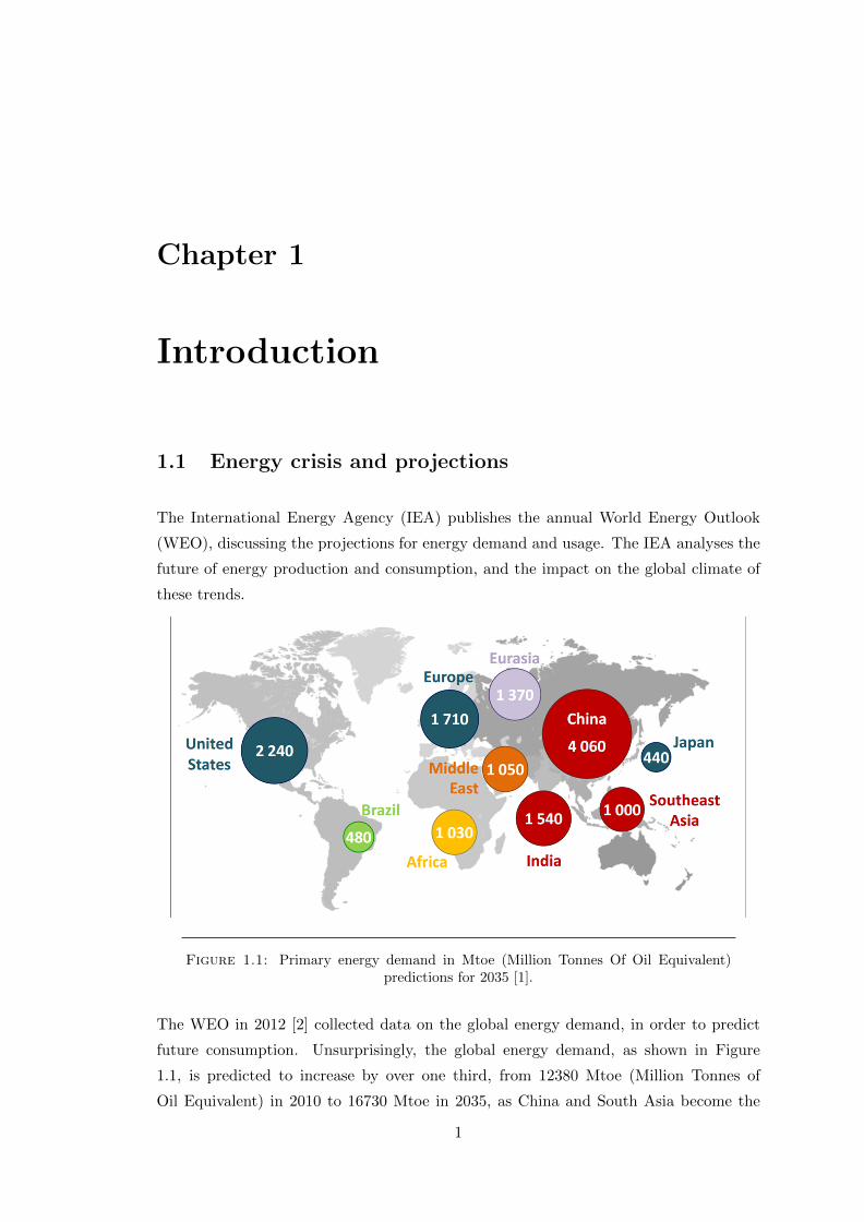
Figure 1.1: Primary energy demand in Mtoe (Million Tonnes Of Oil Equivalent)predictions for 2035 [1].
The WEO in 2012 [2] collected data on the global energy demand, in order to predict
future consumption. Unsurprisingly, the global energy demand, as shown in Figure
1.1, is predicted to increase by over one third, from 12380 Mtoe (Million Tonnes of
Oil Equivalent) in 2010 to 16730 Mtoe in 2035, as China and South Asia become the
1
Chapter 1. Introduction 2
main drivers of energy demand. This drastic increase in energy demand is necessary
for the continued development of many countries, but places increasing strain on global
resources.
With 82% of energy currently generated by burning fossil fuels, the necessity for gov-
ernments to secure diminishing supplies of fossil fuels - and to invest in unconventional
sources such as fracking for shale gas - is unavoidable. The proportion of energy gen-
erated by fossil fuels is the same as 25 years ago- and is projected to drop only as far
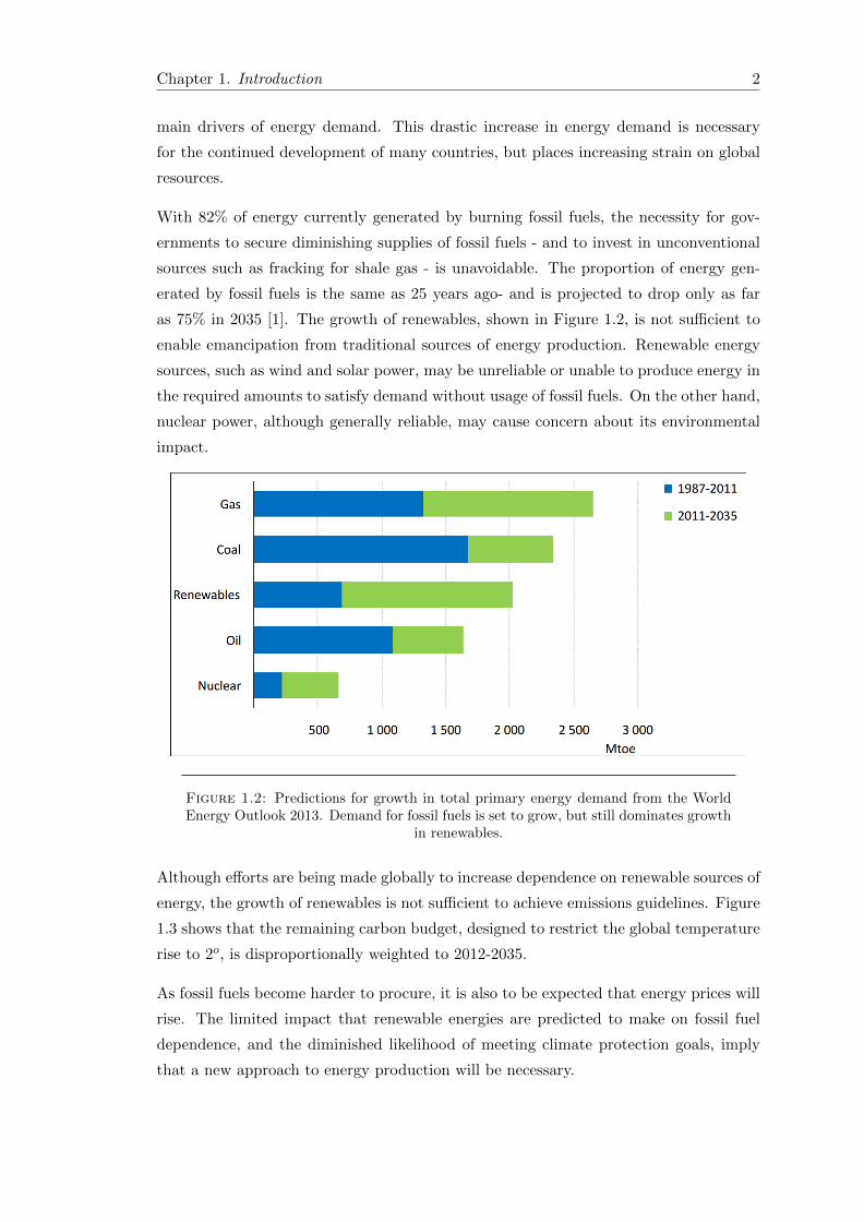
as 75% in 2035 [1]. The growth of renewables, shown in Figure 1.2, is not sufficient to
enable emancipation from traditional sources of energy production. Renewable energy
sources, such as wind and solar power, may be unreliable or unable to produce energy in
the required amounts to satisfy demand without usage of fossil fuels. On the other hand,
nuclear power, although generally reliable, may cause concern about its environmental
impact.
Figure 1.2: Predictions for growth in total primary energy demand from the WorldEnergy Outlook 2013. Demand for fossil fuels is set to grow, but still dominates growth
in renewables.
Although efforts are being made globally to increase dependence on renewable sources of
energy, the growth of renewables is not sufficient to achieve emissions guidelines. Figure
1.3 shows that the remaining carbon budget, designed to restrict the global temperature
rise to 2o, is disproportionally weighted to 2012-2035.
As fossil fuels become harder to procure, it is also to be expected that energy prices will
rise. The limited impact that renewable energies are predicted to make on fossil fuel
dependence, and the diminished likelihood of meeting climate protection goals, imply
that a new approach to energy production will be necessary.

Chapter 1. Introduction 3
Figure 1.3: The carbon budget [1] shows that efforts to minimise climate change havenot significantly impacted dependence on fossil fuels enough to prevent large global
temperature rises.
1.2 Fusion energy
Nuclear power currently uses the fission of heavy elements to generate electricity. How-
ever, at the other end of the binding energy curve, lighter elements which fuse together
release energy. The lighter the element, the more energy is released.
Fusion reactions with the lightest element, hydrogen, occur in the plasma core of the Sun,
producing 3.8× 1026W. The amount of energy released per hydrogen fusion reaction is
substantial, but fusion reactions must involve at least two hydrogen nuclei. These nuclei
must overcome the Coulomb barrier (or, enough of the barrier to increase the probability
of quantum tunnelling) in order to fuse together. Hence fusion reactions require the
involved nuclei to acquire sufficient energy to fuse- in the Sun, the temperature in the
core is over 15 million Kelvin. The fusion environment is one of the most extreme on
Earth.
1.2.1 The Fusion Reaction
To achieve fusion on Earth, it is sensible to choose the fusion reaction with the highest
cross-section, but at achievable energies.
Considering isotopes of hydrogen, there are several fusion reactions which are possible:

Chapter 1. Introduction 4
D2 + T3 → He4 + n1 + 17.6 MeV (1.1)
D2 + D2 → He4 + n1 + 3.27 MeV (1.2)
D2 + D2 → T3 + H1 + 4.03 MeV (1.3)
D2 + He3 → He4 + H1 + 18.3 MeV (1.4)
Deuterium (D2) consists of one proton and one neutron, tritium (T3) of one proton and
two neutrons. The fusion products generally consist of an isotope of helium. The energy
released in each reaction is divided between the velocities of the fusion products. The
cross-sections of these reactions are shown in Figure 1.4.
Figure 1.4: Cross-sections for various fusion reactions as a function of energy [3].Both D-D reaction cross-sections are combined.
The figure shows clearly that the D-T reaction has the highest cross-section, with the
peak around 100keV. The other reactions have comparable cross-sections only at much
higher energies, which would be even more difficult to obtain in any sort of reactor.
Deuterium is found in 0.014-0.015% of natural hydrogen compounds, and is plentiful.
Tritium, on the other hand, is rare and radioactive, with a short half-life of 12.3 years.
However, the neutron produced from the preferred fusion reaction Eq. 1.1 can be used
in a reaction with lithium
Li6 + n1 → He4 + T3 (1.5)
Chapter 1. Introduction 5
in order to produce tritium. Thus, in an operational fusion reactor, tritium can be
manufactured on site.
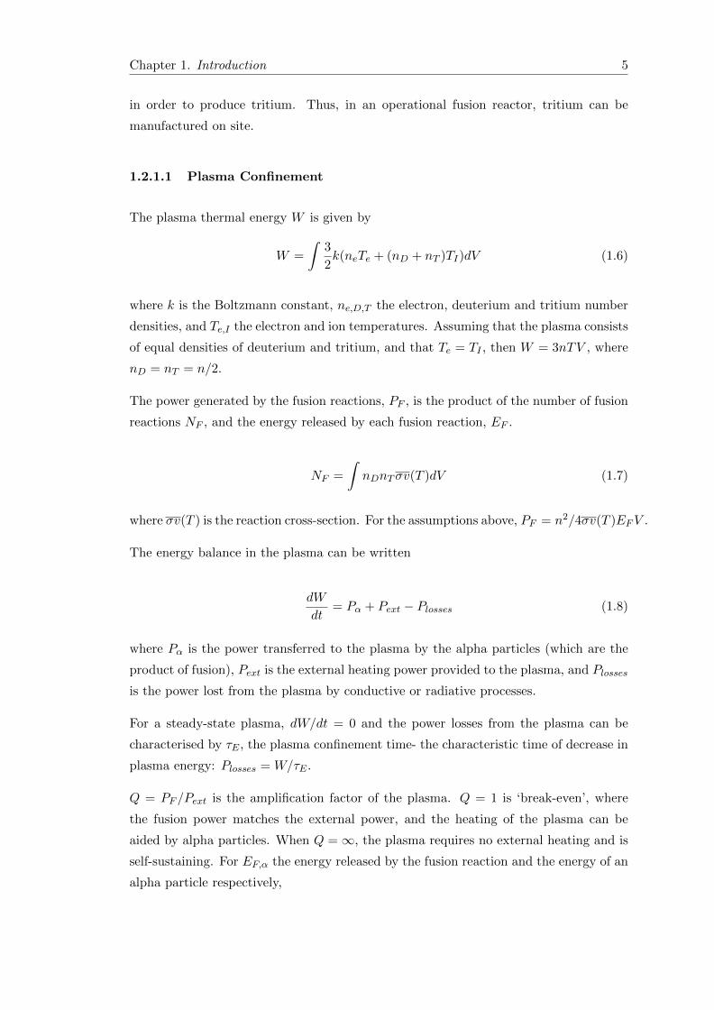
1.2.1.1 Plasma Confinement
The plasma thermal energy W is given by
W =
∫3
2k(neTe + (nD + nT )TI)dV (1.6)
where k is the Boltzmann constant, ne,D,T the electron, deuterium and tritium number
densities, and Te,I the electron and ion temperatures. Assuming that the plasma consists
of equal densities of deuterium and tritium, and that Te = TI , then W = 3nTV , where
nD = nT = n/2.
The power generated by the fusion reactions, PF , is the product of the number of fusion
reactions NF , and the energy released by each fusion reaction, EF .
NF =
∫nDnTσv(T )dV (1.7)
where σv(T ) is the reaction cross-section. For the assumptions above, PF = n2/4σv(T )EFV .
The energy balance in the plasma can be written
dW
dt= Pα + Pext − Plosses (1.8)
where Pα is the power transferred to the plasma by the alpha particles (which are the
product of fusion), Pext is the external heating power provided to the plasma, and Plosses
is the power lost from the plasma by conductive or radiative processes.
For a steady-state plasma, dW/dt = 0 and the power losses from the plasma can be
characterised by τE , the plasma confinement time- the characteristic time of decrease in
plasma energy: Plosses = W/τE .
Q = PF /Pext is the amplification factor of the plasma. Q = 1 is ‘break-even’, where
the fusion power matches the external power, and the heating of the plasma can be
aided by alpha particles. When Q =∞, the plasma requires no external heating and is
self-sustaining. For EF,α the energy released by the fusion reaction and the energy of an
alpha particle respectively,

Chapter 1. Introduction 6
nτE =12kT
σv(T )EF
(EαEF
+ 1Q
) (1.9)
Measuring energy and temperature in keV, EF = 17.6MeV, Eα = 3.6MeV and taking
with Q = ∞ for a self-sustaining plasma, the Lawson criteria [4] can be derived. The
cross section of the D-T fusion reaction between 10-20 keV is ∼ 1.1 × 10⁻²⁴T2m−3s−1.
Thus,
nTτE = 2.6× 10²¹keVm−3s−1 (1.10)
Achieving this value of the triple product nTτE is complicated by the fact that attempt-
ing to increase either n, T or τE may result in a deleterious effect on the other variables.
Progress in fusion research can be demonstrated by the value of nTτE achieved in vari-
ous fusion experiments. In magnetic confinement fusion, the research focus has been on
increasing the confinement time τE .
1.3 Magnetic Confinement Fusion
Due to the high temperatures required for the fusion reaction cross-section to reach
usable levels, the D-T gas will become ionised and the fusion reactions will take place
within a D-T plasma. Thus material walls would be ineffectual for confinement of the
plasma.
In a magnetic field, charged particles gyrate around the magnetic field line, as shown
in Figure 1.5. This provides a means of confinement for the plasma particles, which are
constrained (to first order) to follow the magnetic field lines.
1.3.1 Flux Surfaces
In a tokamak, the plasma is confined by the magnetic field structure. The tokamak is
shaped like a torus: the magnetic field lines loop around the torus in a helical manner.
The magnetic field topology is created by two field components: toroidal and poloidal.
In a conventional tokamak, the toroidal field is generated by toroidal field coils positioned
around the plasma. However, the toroidal field alone is not sufficient to confine the
plasma. The curvature of the tokamak, and the gradient in the magnetic field causes a
tokamak with purely toroidal magnetic field to lose particles (ions and electrons), which

Chapter 1. Introduction 7
Figure 1.5: Charged particles in a magnetic field gyrate around the field line whilstfollowing its trajectory. (Taken from www.efda.org)
drift out of the tokamak. By imposing a poloidal magnetic field, the drifts average to
zero over one poloidal circuit of the plasma. The poloidal magnetic field is generated by
a toroidal plasma current. The resultant magnetic field is shown in Figure 1.6.
Figure 1.6: The combination of toroidal and poloidal magnetic fields results in nestedtoroidal flux surfaces, with helical magnetic field lines confined to one surface.
The topology of the magnetic field in the tokamak is a set of nested toroidal flux surfaces.
The magnetic flux (and plasma pressure) is constant on each surface. Magnetic field
Chapter 1. Introduction 8
lines are confined to one flux surface, and trace a helical path around the tokamak on
that flux surface.
A flux surface can be characterised by the amount of twist a magnetic field line has in
its surface: a field line will migrate both poloidally and toroidally. The safety factor, q,
is a measure of this twist. For one poloidal circuit, a field line will have travelled ∆φ,
and q = ∆φ/2π. If the safety factor is a rational number, then the particles on that
flux surface will, after the requisite number of poloidal and toroidal circuits determined
by the safety factor, loop back to their starting points and retrace their paths. In this
case, the safety factor can be expressed as a ratio of the number of poloidal and toroidal
circuits required to return to the starting point: for example, on a flux surface where
q = 3/2, a particle on that flux surface will have returned to its starting point after
three toroidal and two poloidal circuits. A flux surface with a rational safety factor is
known as a rational surface.
The plasma equilibrium is determined by the Grad-Shafranov equation, which is derived
from the balance between the pressure gradient, and the cross product of the current
density and magnetic field:
R∂
∂R
[1
R
∂ψ
∂R
]+∂2ψ
∂Z2= −µ0R
2 dp
dψ− f df
dψ(1.11)
where ψ is the magnetic flux function, p = p(ψ) the plasma pressure, f = f(ψ) = RBφ
the toroidal field function. R (known as the the major radius, distinct from the minor
radius shown in Figure 1.7), Z and the toroidal angle φ are shown in the tokamak
geometry in Figure 1.7.
Both the plasma pressure p(ψ) and the function f(ψ), along with suitable boundary
conditions, are necessary for solving the Grad-Shafranov equation.
Tokamak Current Drive
The toroidal plasma current, which is necessary for particle confinement, can be gener-
ated inductively or non-inductively. Inductively, it is generated by changing magnetic
flux in the central column, or solenoid, which acts as a transformer. The plasma cur-
rent is also the method for plasma start-up, and provides initial Ohmic heating of the
plasma. However, this method cannot be sustained indefinitely, and is thus unsuited for
non-pulsed operation. But toroidal plasma current can be generated non-inductively.
Neutral beam injection (NBI) systems which fire energetic particles into the tokamak
can drive current, as well as provide heating power for the plasma. Radio-frequency

Chapter 1. Introduction 9
Figure 1.7: The geometry of the tokamak, showing the major (R) and minor (r) radii.The tokamak is often assumed to be symmetric in the toroidal direction.
radiation systems at different frequencies are also capable of driving current and heating
the plasma.
The most enticing method of driving plasma current is one where the plasma generates
its own currents, confining itself. The neoclassical bootstrap current [5, 6] is generated
by collisions between trapped and passing particles: passing particles are those particles
in the plasma which follow a helical path around the tokamak. Trapped particles have an
insufficiently high ratio of parallel to perpendicular components of velocity to traverse
magnetic field maxima caused by the toroidal geometry and cannot complete a full
orbit. These trapped particles follow so-called ‘banana’ orbits. The bootstrap current
is proportional to the radial pressure gradient, and the maximisation of its contribution
to the plasma current would reduce both cost and complexity of a fusion reactor.
Electricity Production
The neutron, as the lighter of the two fusion products, carries 80% of the energy produced
- 14.1 MeV. As the neutron is neutral, it is not held in the magnetic fields of the tokamak.
As it escapes the device, a ‘breeding blanket’ containing lithium is able to firstly, absorb
the neutron energy and create steam to drive turbines; and secondly, produce tritium
in the reaction with lithium. The alpha particle, He4, is confined in the magnetic fields,
and its energy can be used to heat the plasma.

Chapter 1. Introduction 10
1.4 Magnetohydrodynamics In Fusion Plasmas
A plasma, as a collective movement of individual charged particles, can be studied by
using kinetic theory. The distribution function of the particles can be used to investigate
the individual particle movement in the plasma. However, kinetic theory is unable to
capture the large scale collective behaviour of a tokamak plasma. Many of the insta-
bilities which substantially degrade the plasma confinement stem from this collective,
fluid-like behaviour.
In fact, the fluid equations are an obvious starting point for the fluid-like behaviour of a
plasma - the one main difference from the treatment of a neutral fluid being the addition
of a magnetic field term, and the treatment of different particle species. The magnetohy-
drodynamic (MHD) equations are derived from velocity moments of the Vlasov equation
(in the absence of any sources and neglecting collisions):
∂f
∂t+ (v · ∇)f +
1
m(F · ∇v)f = 0 (1.12)
f is the particle distribution function, v the particle velocity, and F the forces on the
particle [3].
1.4.1 MHD Equations
The zeroth moment of Eq. 1.12 is the continuity equation
∂nj∂t
+∇ · (njuj) = 0 (1.13)
j ∈ i, e for ion and electron species, respectively. uj is the flow velocity and nj the
particle density.
The first moment of the Vlasov equation is the force balance equation.
mjnj
[∂uj
∂t+ (uj · ∇)uj
]= −∇pj + njpj(E + uj ×B) (1.14)
for an electric field E, a magnetic field B, pressure pj , and mass mj .
It is possible to continue taking moments of the Vlasov equation indefinitely, but with
each moment, the next highest moment is involved. The zeroth moment involves u,
which is solved for in the first moment. However, the first moment then introduces
Chapter 1. Introduction 11
the pressure pj . The second moment is an equation for pressure, but then requires the
third moment, and so on. In order to close the system, an assumption about one of
the moments has to be made. Usually this assumption is about the pressure, which is
assumed to be adiabatic: for the ratio of specific heats γ, the system is closed by:
[∂
∂t+ (uj · ∇)
](pjn
−γj ) = 0 (1.15)
Combined with the Maxwell equations
∇ ·E =1
ε0(niqi + neqe)
∇×E = −∂B
∂t∇ ·B = 0
∇×B = µ0
[J + ε0
∂E
∂t
]
for species charge qj and current density J. A closed system for uj, pj , nj ,B,E is obtained
[3].
Ideal MHD
A simplification of the MHD equations can be made with several assumptions. These
assumptions may not be appropriate for all situations, but ‘ideal MHD’ is appropriate
for time-scales much larger than the ion cyclotron times, and length scales much larger
than the ion gyro-radius.
Ideal MHD assumes the plasma is a single fluid, combining electrons and ions, and
neglects all dissipative effects such as resistivity, viscosity, and any other collisional
effects.
With the addition of Ohm’s Law
E + u×B = 0 (1.16)
the ideal MHD equations are

Chapter 1. Introduction 12
∂ρ
∂t+∇ · (ρu) = 0
ρ
[∂u
∂t+ (u · ∇)u
]= −∇p+ J×B
∂p
∂t+ (u · ∇)p = −γp∇ · u
∇×B = µ0J∂B
∂t= −∇×E
1.4.2 MHD Instability
Ideal MHD can be used to analyse the (linear) stability of a plasma. The ideal MHD
equations are perturbed and linearised. The perturbation can be expressed as a dis-
placement ξ.
The stability of the plasma is found by examining the plasma energy ∂W . If ∂W > 0
for all displacements, then the plasma is stable. If ∂W < 0 for any displacement ξ, then
the plasma is unstable. Marginal stability corresponds to ∂W = 0.
∂W is comprised of three components: plasma, vacuum, and surface terms. The vacuum
component is always stabilising.
The plasma component ∂Wp can be further decomposed into five terms [3]:
∂Wp =1
2
∫d3x
[|B2
1 |µ0
+B2
µ0|∇·ξ⊥+2ξ⊥·κ|2+γp0|∇·ξ|2−2(ξ⊥·∇p)(κ·ξ∗⊥)−B1·(ξ⊥×b)j||
](1.17)
for κ the curvature vector, b the unit magnetic field vector. The equilibrium and per-
turbation quantities, are differentiated by the subscripts 0 and 1. Vector quantities are
decomposed perpendicular and parallel to the magnetic field lines.
The first three terms correspond to the field line bending, magnetic field compression
and plasma compression contributions. These are always stabilising. The field line
bending term is minimised around flux surfaces with a rational safety factor - hence
MHD instabilities are often localised around rational surfaces. The fourth term is the
driving term for pressure-driven instabilities, and the fifth term the driving term for
current-driven instabilities. The instabilities considered in this thesis are current-driven.

Chapter 1. Introduction 13
Ideal And Resistive Modes
In ideal MHD, the plasma is assumed to be ideal and have no resistivity. This assumption
leads to a significant conclusion: that the plasma and the magnetic field are ‘frozen’
together.
The magnetic field lines and the plasma must evolve in order to conserve flux. This
implies that a change of magnetic topology is not permitted. Magnetic field lines cannot
break and reconnect in an alternate configuration.
If the plasma is permitted to be resistive, then the magnetic field lines can break and
reconnect in a different topology. Additional MHD instabilities are then possible. Insta-
bilities in ideal MHD tend to be the fastest growing and most violent MHD instabilities,
but resistive MHD instabilities usually grow much more slowly and on timescales which
allow for active feedback and mitigation. Tearing modes are resistive MHD instabilities
localised at a rational flux surface.
Internal And External Modes
MHD instabilities can also be categorised by their effect on the plasma boundary. In-
ternal modes are only present inside the plasma, and the plasma boundary remains
stationary. External modes also affect the boundary of the plasma, which can be dis-
torted. For example, the external kink distorts the flux surfaces and requires motion of
the boundary.
1.5 ITER
The next-step international fusion device, ITER [7], being constructed in the south of
France aims to achieve a net output of fusion power. The success of ITER is vital for
the future of fusion power.
ITER will have a tokamak chamber volume eight times that of any previous tokamak,
a major radius R = 6.21m and a minor radius of r = 2.0m, and a schematic is shown
in Figure 1.8. ITER will make significant progress towards the necessary value of the
fusion triple product (Eq. 1.10), as in Figure 1.9.
The dual aims of ITER [8] are, firstly, to demonstrate an amplification factor of Q ≥ 10
for a range of operational scenarios, over a sufficiently long duration; and secondly, to
demonstrate steady-state scenarios with non-inductive current drive for Q ∼ 5. In order
to achieve these goals, ITER will have to produce plasma dominated by alpha particle
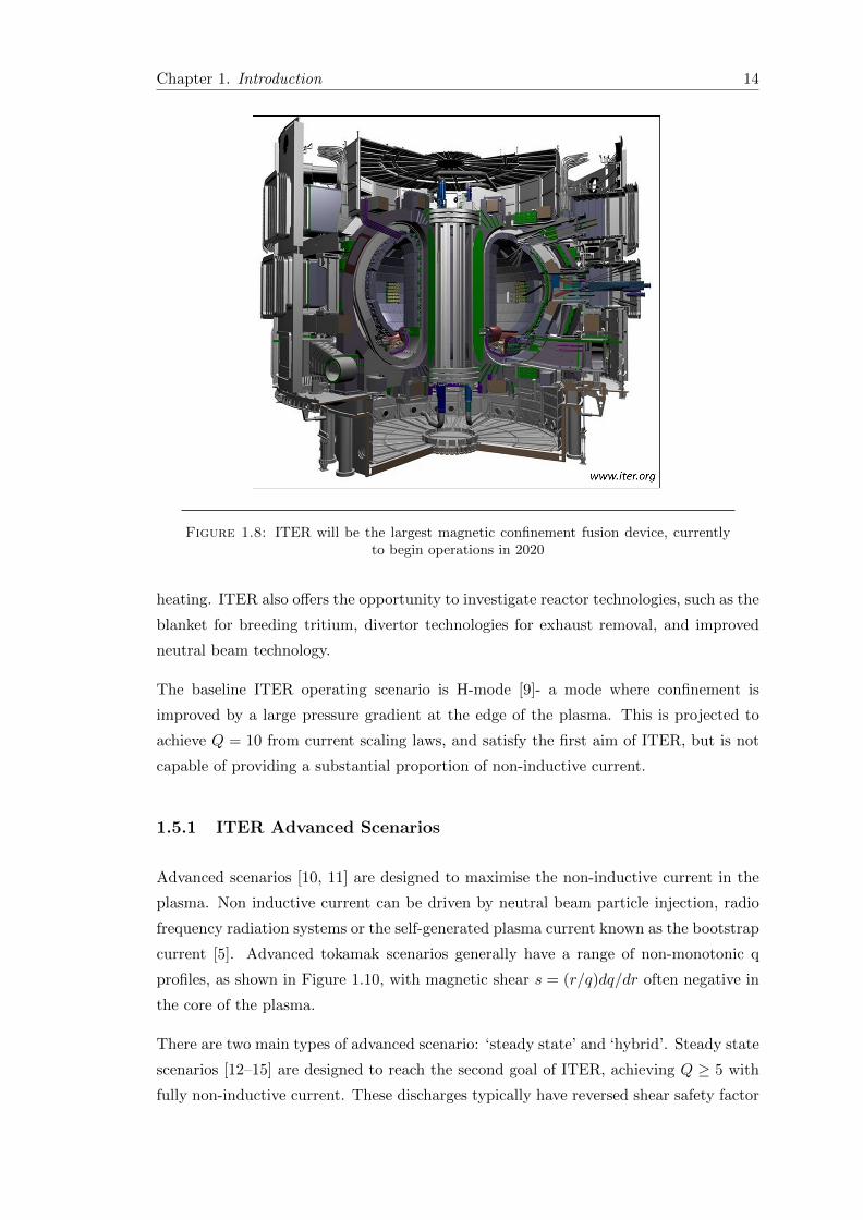
Chapter 1. Introduction 14
Figure 1.8: ITER will be the largest magnetic confinement fusion device, currentlyto begin operations in 2020
heating. ITER also offers the opportunity to investigate reactor technologies, such as the
blanket for breeding tritium, divertor technologies for exhaust removal, and improved
neutral beam technology.
The baseline ITER operating scenario is H-mode [9]- a mode where confinement is
improved by a large pressure gradient at the edge of the plasma. This is projected to
achieve Q = 10 from current scaling laws, and satisfy the first aim of ITER, but is not
capable of providing a substantial proportion of non-inductive current.
1.5.1 ITER Advanced Scenarios
Advanced scenarios [10, 11] are designed to maximise the non-inductive current in the
plasma. Non inductive current can be driven by neutral beam particle injection, radio
frequency radiation systems or the self-generated plasma current known as the bootstrap
current [5]. Advanced tokamak scenarios generally have a range of non-monotonic q
profiles, as shown in Figure 1.10, with magnetic shear s = (r/q)dq/dr often negative in
the core of the plasma.
There are two main types of advanced scenario: ‘steady state’ and ‘hybrid’. Steady state
scenarios [12–15] are designed to reach the second goal of ITER, achieving Q ≥ 5 with
fully non-inductive current. These discharges typically have reversed shear safety factor
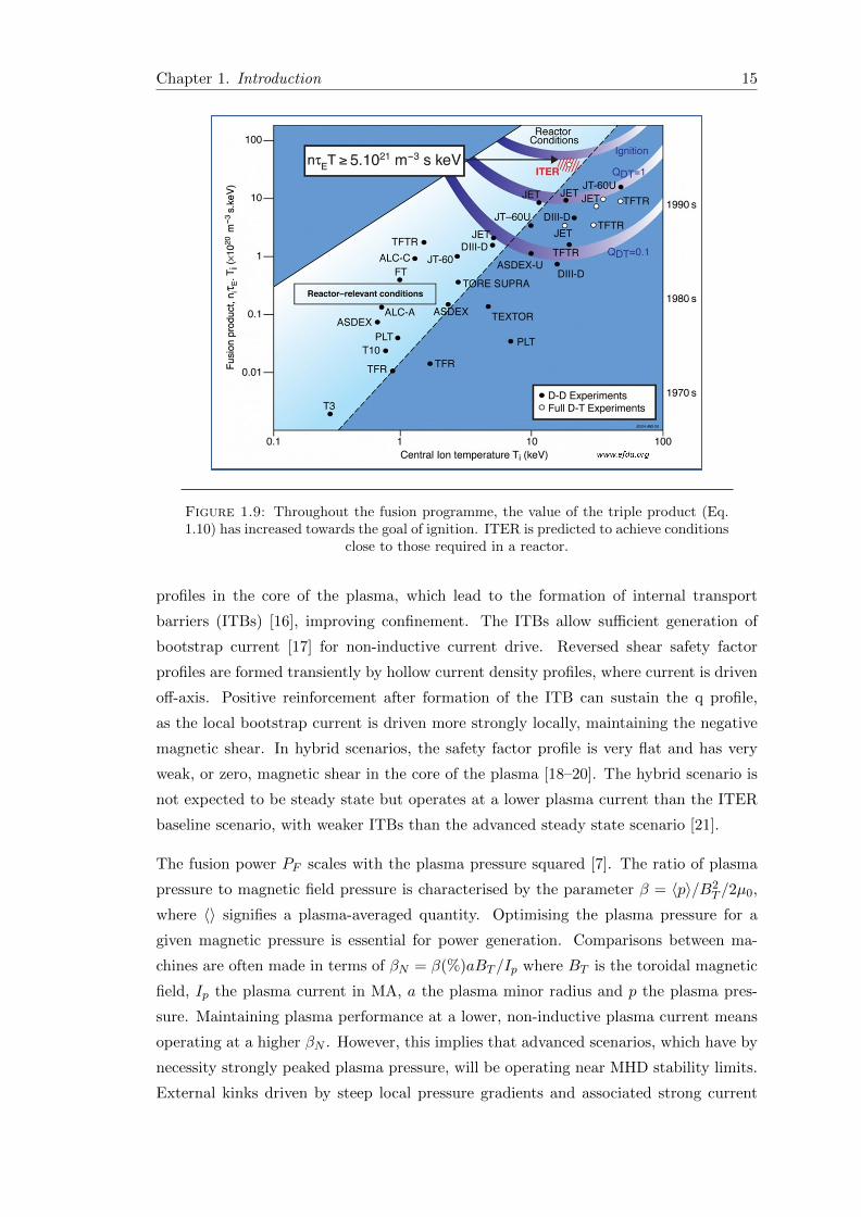
Chapter 1. Introduction 15
Figure 1.9: Throughout the fusion programme, the value of the triple product (Eq.1.10) has increased towards the goal of ignition. ITER is predicted to achieve conditions
close to those required in a reactor.
profiles in the core of the plasma, which lead to the formation of internal transport
barriers (ITBs) [16], improving confinement. The ITBs allow sufficient generation of
bootstrap current [17] for non-inductive current drive. Reversed shear safety factor
profiles are formed transiently by hollow current density profiles, where current is driven
off-axis. Positive reinforcement after formation of the ITB can sustain the q profile,
as the local bootstrap current is driven more strongly locally, maintaining the negative
magnetic shear. In hybrid scenarios, the safety factor profile is very flat and has very
weak, or zero, magnetic shear in the core of the plasma [18–20]. The hybrid scenario is
not expected to be steady state but operates at a lower plasma current than the ITER
baseline scenario, with weaker ITBs than the advanced steady state scenario [21].
The fusion power PF scales with the plasma pressure squared [7]. The ratio of plasma
pressure to magnetic field pressure is characterised by the parameter β = 〈p〉/B2T /2µ0,
where 〈〉 signifies a plasma-averaged quantity. Optimising the plasma pressure for a
given magnetic pressure is essential for power generation. Comparisons between ma-
chines are often made in terms of βN = β(%)aBT /Ip where BT is the toroidal magnetic
field, Ip the plasma current in MA, a the plasma minor radius and p the plasma pres-
sure. Maintaining plasma performance at a lower, non-inductive plasma current means
operating at a higher βN . However, this implies that advanced scenarios, which have by
necessity strongly peaked plasma pressure, will be operating near MHD stability limits.
External kinks driven by steep local pressure gradients and associated strong current

Chapter 1. Introduction 16
Figure 1.10: A wide range of q profiles can be obtained in the tokamak. Profileswith reversed magnetic shear in the core of the plasma are associated with advanced
scenarios of operation[11]
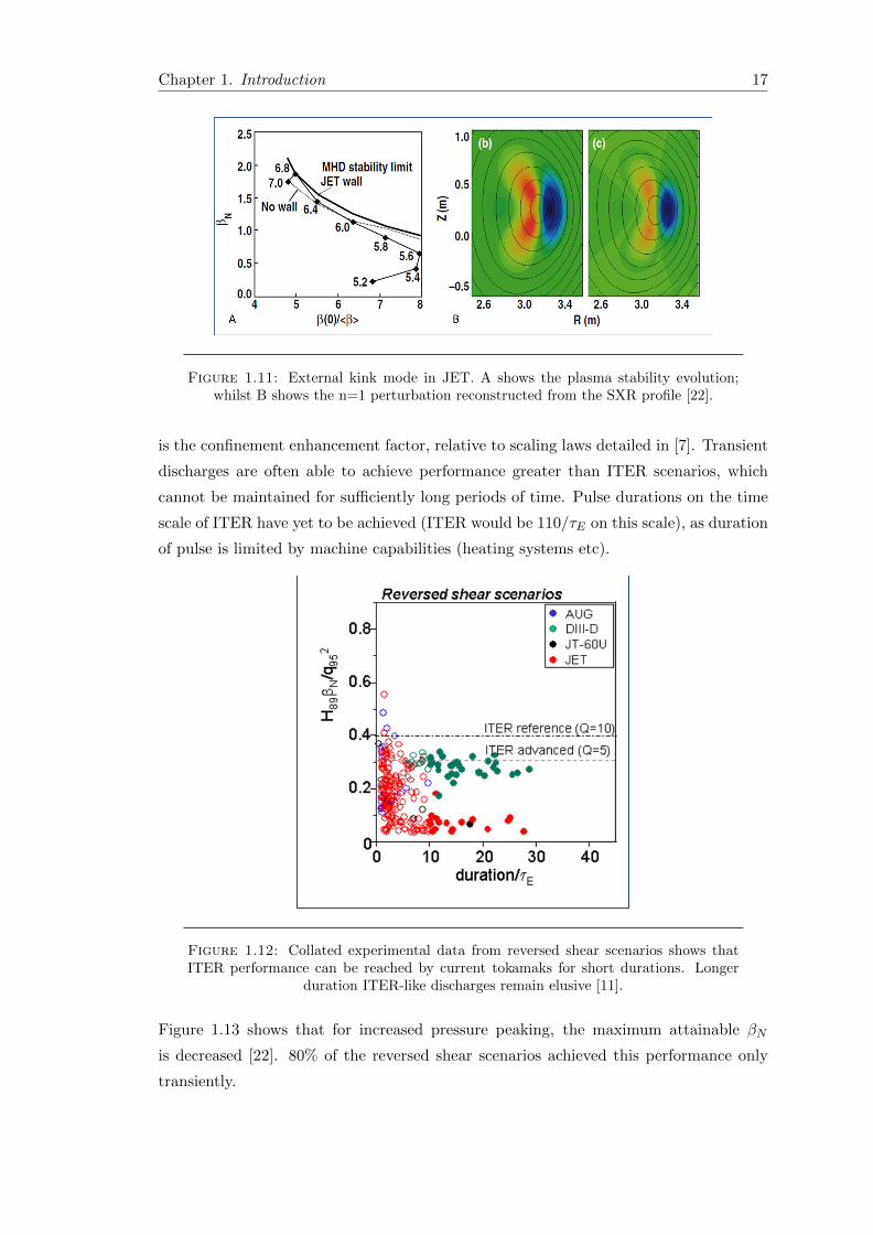
density can be destabilised. Kink stability limits achievable βN in a reactor, and hence
the fusion performance. Figure 1.11 shows an external kink mode in JET [22], mapped
by the soft x-ray signals. Figure 1.11a) shows the plasma discharge through phase space:
the plasma crosses the no-wall beta limit and moves towards the ideal wall-wall limit.
This destabilises the external kink mode, the reconstruction of the soft x-ray emissions
profile is in Figure 1.11b) compared to ideal MHD calculations in c).
The external kink is destabilised when βN > 4li, in the absence of a resistive wall, where
li is known as the plasma inductance, and 4lii is often used as an experimental proxy
for the external kink stability limit. The stability limit is measured by the plasma βN :
if a plasma has no surrounding wall, then the βN at which the external kink becomes
unstable is known as the no-wall limit. If the plasma is surrounded by a superconducting
wall, then the external kink can be stabilised over a wider range of βN by bringing the
superconducting wall sufficiently close to the plasma. This raises the stability limit to
the ideal-wall limit: βideal−wallN > βno−wallB . If the wall is resistive, then an unstable mode
is still present and is known as the Resistive Wall Mode [23]. The mode is unstable for
βN greater than the no-wall limit, but the presence of the resistive wall slows its growth
to a rate dependant on the resistivity of the wall. Reversed shear plasmas have a plasma
inductance of li ∼ 0.8, severely limiting the achievable βN .
Fig 1.12 shows experimental progress in reversed shear scenarios-H89βN/q295 is a measure
of plasma performance, with ITER reference scenarios’ performances indicated [11]. H89
Chapter 1. Introduction 17
Figure 1.11: External kink mode in JET. A shows the plasma stability evolution;whilst B shows the n=1 perturbation reconstructed from the SXR profile [22].
is the confinement enhancement factor, relative to scaling laws detailed in [7]. Transient
discharges are often able to achieve performance greater than ITER scenarios, which
cannot be maintained for sufficiently long periods of time. Pulse durations on the time
scale of ITER have yet to be achieved (ITER would be 110/τE on this scale), as duration
of pulse is limited by machine capabilities (heating systems etc).
Figure 1.12: Collated experimental data from reversed shear scenarios shows thatITER performance can be reached by current tokamaks for short durations. Longer
duration ITER-like discharges remain elusive [11].
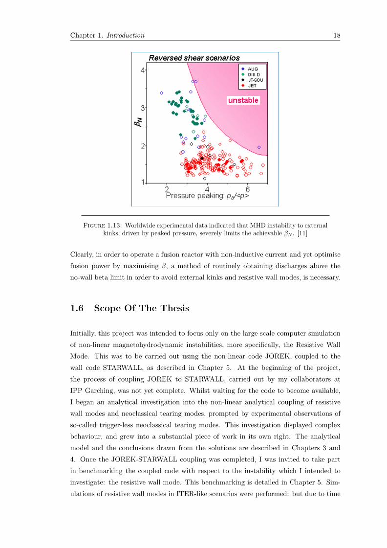
Figure 1.13 shows that for increased pressure peaking, the maximum attainable βN
is decreased [22]. 80% of the reversed shear scenarios achieved this performance only
transiently.
Chapter 1. Introduction 18
Figure 1.13: Worldwide experimental data indicated that MHD instability to externalkinks, driven by peaked pressure, severely limits the achievable βN . [11]
Clearly, in order to operate a fusion reactor with non-inductive current and yet optimise
fusion power by maximising β, a method of routinely obtaining discharges above the
no-wall beta limit in order to avoid external kinks and resistive wall modes, is necessary.
1.6 Scope Of The Thesis
Initially, this project was intended to focus only on the large scale computer simulation
of non-linear magnetohydrodynamic instabilities, more specifically, the Resistive Wall
Mode. This was to be carried out using the non-linear code JOREK, coupled to the
wall code STARWALL, as described in Chapter 5. At the beginning of the project,
the process of coupling JOREK to STARWALL, carried out by my collaborators at
IPP Garching, was not yet complete. Whilst waiting for the code to become available,
I began an analytical investigation into the non-linear analytical coupling of resistive
wall modes and neoclassical tearing modes, prompted by experimental observations of
so-called trigger-less neoclassical tearing modes. This investigation displayed complex
behaviour, and grew into a substantial piece of work in its own right. The analytical
model and the conclusions drawn from the solutions are described in Chapters 3 and
4. Once the JOREK-STARWALL coupling was completed, I was invited to take part
in benchmarking the coupled code with respect to the instability which I intended to
investigate: the resistive wall mode. This benchmarking is detailed in Chapter 5. Sim-
ulations of resistive wall modes in ITER-like scenarios were performed: but due to time
Chapter 1. Introduction 19
restrictions for the completion of this thesis, simulations which investigate the behaviour
of neoclassical tearing modes in the RWM-unstable plasma were not able to be included
in Chapter 6. Further work would investigate the inclusion of NTMs in these simulations
in order to expand the analytical work.

Chapter 2
Literature Review
2.1 Resistive Wall Modes In Tokamak Plasmas
One of the main magneto-hydrodynamic instabilities limiting the achievable β in toka-
mak plasmas - particularly advanced scenario plasmas - is the external n=1 kink mode,
with n the toroidal mode number [10]. The external kink is an ideal MHD mode with
global structure, which results in significant plasma displacement at the boundary of the
plasma.
2.1.1 Resistive Walls
For an external MHD mode, the plasma boundary is displaced. The flux perturbation
associated with the instability extends beyond the plasma boundary into the vacuum
region outside the plasma. The presence of an external wall thus has some effect on any
external flux perturbation intercepted by the wall.
For an ideal (superconducting) wall, the magnetic flux is unable to diffuse through the
wall. This has the effect of ‘pinning’ the flux perturbation to the wall boundary and
providing stabilisation for the mode, as shown in Figure 2.1.
However, tokamak plasmas are not surrounded by superconducting walls. Current walls
have finite resistivity. Resistive walls are somewhat stabilising, as some magnetic flux is
still able to permeate the wall. This change in boundary conditions causes the growth
rate, and the marginal stability of the mode, to change.
It has been found numerically [24] that the tokamak operational envelope was limited by
a value of βN = 2.8. Above this limit, the plasma was found to be unstable. This limiting
20

Chapter 2. Literature Review 21
Figure 2.1: An ideal wall prevents flux perturbations diffusing through it, providingstabilisation for the mode.
βN was calculated with the assumption of no external conducting wall. In a steady-
state reactor, any wall stabilisation would be ineffective over the discharge lifetime.
Experimentally, the βN limit, shown in Figure 2.2, was found to be βexpN ∼ 3.5 [25],
indicating that the external wall does exert a stabilising influence in current tokamak
discharges.
Figure 2.2: Comparison of experimental βT with normalised current. The operationalenvelope is bounded by βN = 3.5 [26]

Chapter 2. Literature Review 22
The radius of the wall location is also crucial in the mode stability. If the plasma,
subject to an external kink, is surrounded by a wall at infinity (or sufficiently far from
the plasma that it is perceived to be ‘at infinity’), then the external kink is unstable
for βN > βno−wallN . βno−wallN is the stability boundary for the external kink. If an ideal
wall is brought towards the plasma, then at a certain radius, the external kink will be
stabilised and the stability boundary is raised such that the plasma is additionally stable
for βno−wallN < βN < βidealN . The situation is illustrated in Figure 2.3.
Consider now a (non-rotating) plasma which has finite resistivity. It has been proven [27]
that any MHD unstable plasma configuration with dissipation-less plasma, surrounded
by a vacuum and possibly superconducting walls, cannot be stabilised by adding walls of
finite resistivity around the plasma. The growth rate of the mode can only be reduced to
τ−1w , where τw is the characteristic time scale for the magnetic flux to diffuse through the
wall. This time scale is derived in Section 3.3.1. In DII-D, τw is found experimentally
to be 5− 7ms [28]. Typically, the growth rate without a wall is on the time-scale of the
much faster Alfven time τA.
The Resistive Wall Mode (RWM) is the branch of the external kink instability which is
excited when the plasma is surrounded by a wall of finite resistivity, and is unstable for
βno−wallN < βN < βidealN . Like the external kink, it is a global mode, which additionally
has a low frequency. As discussed in Chapter 1, the RWM is likely to be destabilised for
advanced tokamak scenarios which need to operate at high βN , with peaked pressure
profiles.
Figure 2.3: [29] Stability limits for external kink.
2.2 RWM Dispersion Relation
A useful treatment of the Resistive Wall Mode is using the variational method to derive
the dispersion relation for the mode, which can be used to track the mode stability as
the boundary conditions are changed. This is demonstrated by Haney and Freidberg in
[30]. The derivation of the results is shown in more detail in Appendix A. The dispersion
relation
Chapter 2. Literature Review 23
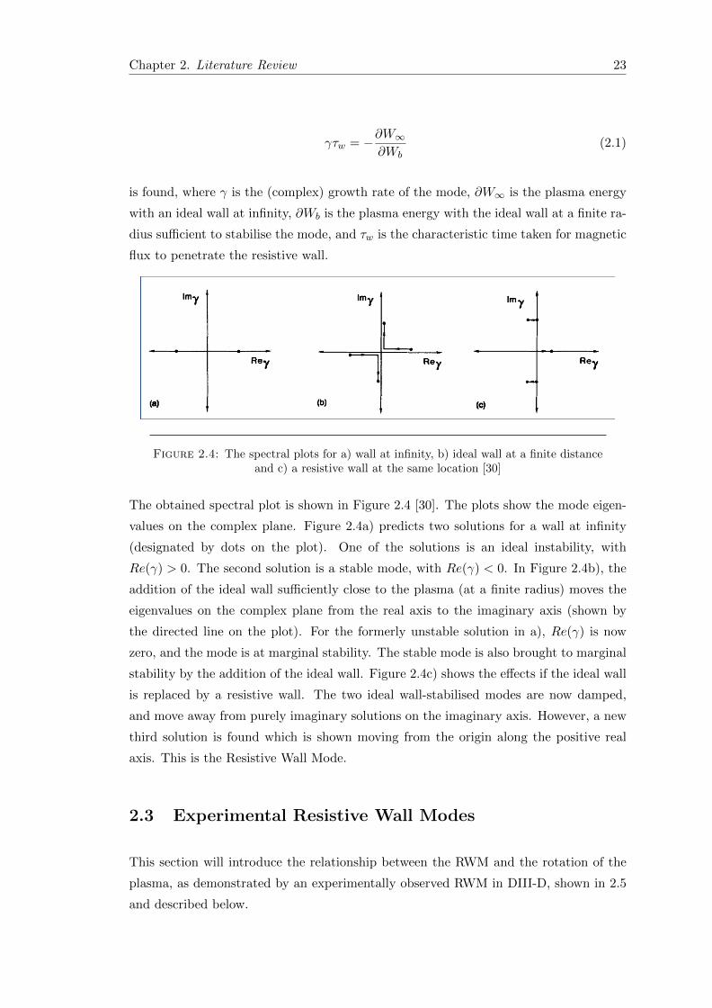
γτw = −∂W∞∂Wb
(2.1)
is found, where γ is the (complex) growth rate of the mode, ∂W∞ is the plasma energy
with an ideal wall at infinity, ∂Wb is the plasma energy with the ideal wall at a finite ra-
dius sufficient to stabilise the mode, and τw is the characteristic time taken for magnetic
flux to penetrate the resistive wall.
Figure 2.4: The spectral plots for a) wall at infinity, b) ideal wall at a finite distanceand c) a resistive wall at the same location [30]
The obtained spectral plot is shown in Figure 2.4 [30]. The plots show the mode eigen-
values on the complex plane. Figure 2.4a) predicts two solutions for a wall at infinity
(designated by dots on the plot). One of the solutions is an ideal instability, with
Re(γ) > 0. The second solution is a stable mode, with Re(γ) < 0. In Figure 2.4b), the
addition of the ideal wall sufficiently close to the plasma (at a finite radius) moves the
eigenvalues on the complex plane from the real axis to the imaginary axis (shown by
the directed line on the plot). For the formerly unstable solution in a), Re(γ) is now
zero, and the mode is at marginal stability. The stable mode is also brought to marginal
stability by the addition of the ideal wall. Figure 2.4c) shows the effects if the ideal wall
is replaced by a resistive wall. The two ideal wall-stabilised modes are now damped,
and move away from purely imaginary solutions on the imaginary axis. However, a new
third solution is found which is shown moving from the origin along the positive real
axis. This is the Resistive Wall Mode.
2.3 Experimental Resistive Wall Modes
This section will introduce the relationship between the RWM and the rotation of the
plasma, as demonstrated by an experimentally observed RWM in DIII-D, shown in 2.5
and described below.
Chapter 2. Literature Review 24
2.3.1 Resistive Wall Modes And Plasma Rotation
The RWM has a complex, non-linear relationship with the plasma rotation, and RWM
theory has centred around rotational stabilisation in dissipational plasmas in many mod-
els. If the wall surrounding the plasma is ideal, then due to the conservation of flux in
an ideal medium, the perturbed magnetic flux cannot penetrate the ideal wall. If the
wall is resistive, the flux is then able to penetrate the wall. However, if the plasma and
the resistive wall can be made to rotate relative to each other, any single location on the
wall will experience a constantly changing phase in the perturbed magnetic flux. The
magnetic flux does not have the opportunity to penetrate the wall. In the plasma frame
of reference, the wall appears to be ideal and is stabilising. Hence, in Figure 2.5, the
crucial destabilising factor is the loss of plasma rotation.
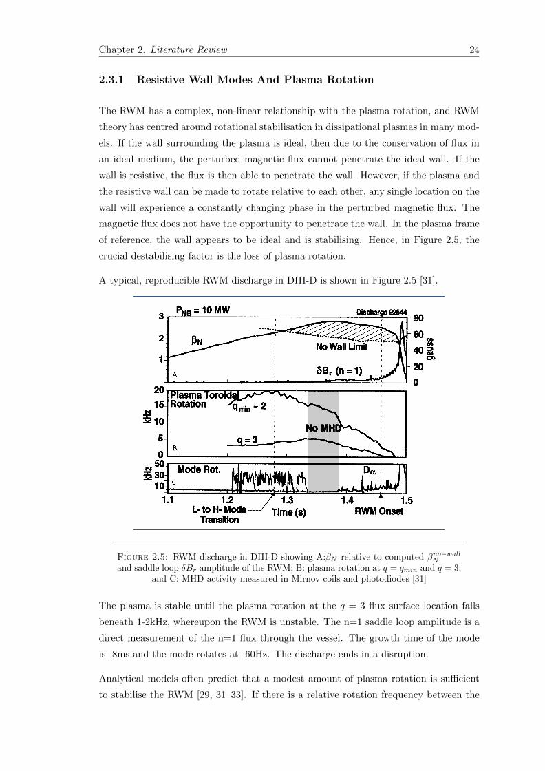
A typical, reproducible RWM discharge in DIII-D is shown in Figure 2.5 [31].
Figure 2.5: RWM discharge in DIII-D showing A:βN relative to computed βno−wallN
and saddle loop δBr amplitude of the RWM; B: plasma rotation at q = qmin and q = 3;and C: MHD activity measured in Mirnov coils and photodiodes [31]
The plasma is stable until the plasma rotation at the q = 3 flux surface location falls
beneath 1-2kHz, whereupon the RWM is unstable. The n=1 saddle loop amplitude is a
direct measurement of the n=1 flux through the vessel. The growth time of the mode
is 8ms and the mode rotates at 60Hz. The discharge ends in a disruption.
Analytical models often predict that a modest amount of plasma rotation is sufficient
to stabilise the RWM [29, 31–33]. If there is a relative rotation frequency between the
Chapter 2. Literature Review 25
mode and the wall, then in the frame of reference of the mode the wall appears as an
ideal wall. Thus the magnetic flux perturbations do not penetrate the wall. Conversely,
both experiment and theory show that drag associated with the RWM will damp plasma
rotation [31, 34]. This is due to the eddy currents induced in the resistive wall by the
magnetic perturbations.
2.4 Resistive Wall Modes And Nonlinear Effects
Although the RWM can be analysed linearly, as will be described in Chapter 5, it is the
non-linear contributions to RWM stability that are found to be extremely important.
The non-linear interaction with the toroidal plasma rotation is an important stabilisation
mechanism. Non-linear-coupling to other MHD modes is also a factor in RWM stability.
2.4.1 Plasma Rotation
In Resistive Wall Mode theory, RWM stabilisation by plasma rotation Ω relative to the
resistive wall is characterised in three ways by Gimblett and Hastie [35]
1. A stability window in plasma rotation, ∃Ω1,Ω2 such that the RWM is stable for
Ω1 < Ω < Ω2
2. A critical rotation Ωcrit such that the RWM is stable for Ω > Ωcrit
3. The RWM is never stabilised, only mitigated
Theoretical models which seek to calculate the stabilisation of the external kink provided
by resistive walls require a source of dissipation in the plasma.
2.4.2 Theoretical RWM Stabilisation Models
Numerical Study Of Bondeson And Ward
The first study of rotational stabilisation was Bondeson and Ward [36].
The numerical study proposed that low n, pressure driven external kink modes could
be fully stabilised when the plasma rotates at some fraction of the sound speed. The
mechanism for transferring momentum from the plasma to the mode is toroidal coupling
to sound waves, via ion Landau damping. Two modes were found, the plasma mode

Chapter 2. Literature Review 26
Figure 2.6: A stability window for a rotating plasma appears such that both the idealplasma mode and the resistive mode are stable [29, 36].
rotating with the plasma, and the resistive mode penetrating the wall and nearly locked
to it. A window of stability for both modes appears. The resistive mode is more stable
as the resistive shell moves further from the plasma boundary, whereas the plasma
mode is more stable if the shell approaches the plasma. The stability of the modes can
be seen in Figure 2.6 for a plasma pressure 30% above the no-wall limit, rotating at
Ω/ωA = 0.06, where Ω is the plasma rotation frequency, and ωA is the Alfven frequency.
When the frequency of the RWM with respect to the wall is large, the RWM is stabilised.
For the minor radius a, and wall radius d, the stability window for a resistive wall is
1.4 < d/a < 1.7.
[36] gives the following explanation for RWM stabilisation. If the plasma is rotating,
then the energy flux [37]
∂Wp =1
2
∫Sp
ξ∂ξ
∂xdS (2.2)
is complex. This means that the perturbed radial and poloidal magnetic field compo-
nents have a relative phase shift. The perturbed flux is proportional to the displacement,
so the idea of energy flux can be expressed in terms of the perturbed flux ψ. The magnetic
flux function ψ is defined by Br = − 1R∂ψ∂Z and BZ = 1
R∂ψ∂R . In linear stability analyses,
the necessary quantity is the logarithmic derivative of ψ. At the plasma boundary r = a,
[36] requires
ψ′
ψ
∣∣∣∣a
= −ma
(1 + x+ iy) (2.3)

Chapter 2. Literature Review 27
where m is the poloidal mode number. The real part, ∼ (1+x) means that the perturbed
magnetic field transfers energy through the plasma boundary, where 1 signifies marginal
stability, and x signifies an excess or a deficit of energy. The imaginary component
represents the angular momentum carried by the perturbed field through the boundary.
If the plasma is stationary, then ψ′/ψ →∞ at the ideal wall stability boundary. If the
plasma is rotating, then ψ′/ψ must remain finite and complex at any wall distance. The
rotation of the plasma separates the plasma and the resistive modes from each other. In
a rotating plasma, the perturbed plasma current Ip would force the perturbed induced
wall currents Iw to rotate with respect to the wall. Hence Ip and Iw cannot grow in
phase with each other, leading to stabilisation.
One limitation of this model is that the numerical code used to calculate the results
modelled a stationary plasma with a rotating resistive shell, so the effect of flow shear
could not be explored.
Analytical Studies For Cylindrical Plasmas
Analytical models for the stabilisation of RWMs were also proposed as a reaction to
[36]. Betti and Freidberg [38] utilised a cylindrical model where mode resonance with
the sound wave continuum opens up a stability window for the RWM, with a cubic
dispersion relation. Adding toroidal effects increases the dissipation in the model. These
results are able to explain the numerical work in [36].
[39] uses a simple cylindrical model with dissipation provided by edge plasma viscosity.
In both [38] and [39], the critical rotation was found to be of the order k||avA, where k||
is the parallel wave number of the RWM at the edge of the plasma, and vA the Alfven
speed. The external kink is unstable for k||a << 1 for low n kink modes, so the critical
rotation velocity is only a few percent of the Alfven speed - velocities regularly reached
by neutral beam injection in tokamaks.
The results in [39] agree well with those in [36, 38] despite the difference in dissipation
mechanism. Indeed, once the stability window in βT , where βT is the plasma parameter
β measured using only the toroidal magnetic field instead of the full magnetic field, is
sufficiently large, the dissipation mechanism is unimportant. As long as both plasma
rotation and a dissipation mechanism are both present, a stability window exists.
Finn also studied this problem [40], but with a different stabilisation mechanism. In
contrast to the previously discussed models, this study includes a resistive plasma. For a
cylindrical plasma with infinite aspect ratio, with resistive wall and rigid plasma rotation,
an external resonant ideal MHD mode with a rational surface in the plasma is considered.
Chapter 2. Literature Review 28
This ideal mode, unstable with a wall at infinity but stabilised by a conducting wall,
can be stabilised by becoming resistive modes, which allow a change in the magnetic
topology. The resistive modes can then be stabilised by the resistive wall and bulk
plasma rotation. Resistive modes imply the possible development of magnetic islands at
the rational surface, which can transfer momentum to the RWM. The critical rotation
frequency for stabilisation is lower than the previous models, at << 1% of the Alfven
frequency. The use of a resistive plasma was also examined in [41] for a circular plasma.
Confirming the results in [40], [42] looked at a single mode rational surface in the plasma
with the resistive kink dispersion relation [43]. The ideal mode can be stabilised by a
close wall and plasma rotation on similar time scales to those found in [40], in a small
parameter range.
2.4.3 Torque Balance In A Tokamak
The rotation profile in the tokamak plasma is determined by three factors
1. The natural rotation tendency of the plasma [44, 45]
2. External torque input (Neutral Beam Injection or EM interaction with external
wall and error fields)
3. Inter-flux surface viscosity
The torque induced by a resistive instability and an external resistive wall is examined
in [46]. The importance of the rotation of MHD modes and torque balance between
the plasma and the resistive wall in the stability of the plasma was pointed out by
Hender et al. [47]. Further studies [48–50] confirmed the importance of torque balance
as bifurcated states for the plasma equilibrium were discovered.
2.4.4 Rotation Threshold Experiments
The importance of the inclusion of torque balance in consideration of the rotation thresh-
old for RWM stabilisation can be seen in a series of experiments.
Initially, experiments on DIII-D and JT-60U [31, 51, 52] found relatively high values of
plasma rotation were needed to stabilise the resistive wall mode. The experiments are
carried out by using Neutral Beam Injection (NBI) to impart torque into the plasma, and
magnetic braking (applying an external resonant non-axisymmetric field) to decelerate

Chapter 2. Literature Review 29
the plasma. When the plasma rotation crosses the RWM stabilisation threshold, the
RWM begins to grow.
However, other experiments [53, 54] found a much lower rotation threshold. These
experiments used a different method to ascertain the rotation threshold, using much less
NBI. An example is shown in Figure 2.7. Controlling the NBI torque with a system
of co- and counter-rotation beams, non-axisymmetric magnetic braking fields are not
needed to brake the plasma. Non-axisymmetric fields are minimised while the initial
NBI torque is reduced until the q=2 rotation is at the level of ΩτA ∼ 0.3%. This is a
much lower threshold than found in previous experiments with braking fields and fixed
NBI injection. Varying the NBI also has a significant effect on the rotation profiles
in Figure 2.7d), such that rotation at just one rational surface may not be sufficient
information to analyse the stabilisation of the RWM.
The reconciliation of these different rotation thresholds lies in the torque balance of
the plasma. At the mode rational surface (q=2) in external braking experiments, it has
been noticed that firstly there was a slow deceleration in rotation with an increase in the
external field. After this initial slow phase, a rapid drop in rotation where the magnetic
perturbation transitions to a higher growth phase is noticed: the transition from slow
to fast RWM growth is illustrated in Figure 2.8.
The transition between slow and fast RWM growth was thought to be the RWM rotation
stabilisation threshold. In fact, it is due to a bifurcation in the torque balance equilibrium
where the rotation jumps from a high to a low value. The actual RWM threshold may
be in the intervening band of rotation values. The bifurcation phenomenon is explained
in [50]. The rotational drag caused by the applied field has a non-monotonic dependence
on the plasma rotation, due to electromagnetic shielding of the error field at the rational
surface as the rotation increases. This results in greater RWM stabilisation and a smaller
response from the applied field. If the plasma is subjected to high NBI torque, then there
is a high unperturbed plasma rotation value, and hence a higher value of rotation at
the upper entrance to the forbidden rotation band. At the bifurcation point, the eddy
currents on the rational surface no longer shield the plasma from the static applied field,
and there is a transition from the shielded to the fully penetrated braking field. The
rotation collapses to near locking values.
In plasma shots where there is a large initial plasma rotation, the plasma rotation will
undergo the bifurcation when the magnetic braking is applied. In DIII-D, the strong NBI
torque and the large unperturbed plasma rotation combined with the strong magnetic
braking causes the bifurcation in the torque balance. This leads to sudden decreases
in rotation and increases in RWM amplitude. With initially small NBI torque and no
magnetic braking, the plasma should be able to reach the true MHD stability boundary.

Chapter 2. Literature Review 30
Figure 2.7: [53]a) shows βN and ∂Br amplitude of the non-rotating n=1 RWM, b)NBI torque, c) toroidal velocity at several ρ = r/a locations and d) rotation profiles at
various discharge times.
Hence, there is a certain level of uncertainty in the exact value of the rotation threshold
for RWM growth, both experimentally and theoretically. Different models predict differ-
ent thresholds, and even different approaches to braking and reduction of plasma torque
in experiments yields different results. The threshold for rotational RWM stabilisation
is thus also very machine dependant, which makes predictions of performance in future
machines, such as ITER, challenging.

Chapter 2. Literature Review 31
Figure 2.8: [34] Two experimental discharges in DIII-D with differing initial NBItorque. The figure shows a)βN (solid curve), the no-wall limit approximation and thenumber of NBI sources, b) n=1 ∂Br amplitude at the sensor loops, c) plasma toroidalrotation at r/a ≈ 0.6 and d) rotation profiles at t=1.2s shows faster initial rotationfor the discharge with greater torque input, while in e) at the transition to fast RWMgrowth and slow plasma rotation (vertical lines in a,b,c) the profiles are identical inboth discharges. The discharge with greater initial torque survives longer before the
transition from slow to fast RWM growth.
2.4.5 Torque Balance Models For The RWM
It was noticed experimentally that reducing error fields could lengthen discharges, as
the drag on the plasma was reduced and rotation increased [31]. This (non-linear)
effect on the plasma can be captured analytically by including the torque balance of
the plasma. However, in the previous studies mentioned, the plasma rotation was not
included self-consistently in the models.
In [55], Gimblett and Hastie used the Finn model [40] to show the magnetic island
transferring momentum between the wall and the plasma: this provides a means to self
consistently include, in a non-linear way, the plasma rotation in the model. In terms of
RWM stability, the necessity of allowing the growth of the magnetic island is mitigated

Chapter 2. Literature Review 32
by a larger region in parameter space where the RWM is stable. Self-consistent torque
balance for external error fields was also studied by Fitzpatrick in [56].
In [35], torque balance was used to analyse a plasma affected by error fields (fields caused
by misaligned coils). A braking effect on the plasma rotation caused by the error field
is shown, and that reducing the error field amplitude will lengthen plasma discharges,
which agrees with the experimental work on DIII-D [31]. Variants of this model also
help understand the forbidden bands of rotation seen in [57].
The work described in [35, 55] is notable here because the structural mathematical
framework which is used is similar that used in 3. A short summary of the model is
included in Appendix B.
2.4.6 Other Effects On Resistive Wall Modes
External Fields
If the RWM is destabilised, it is possible to stabilise the plasma by implementing a
feedback system. This was initially suggested in [58]. The principle is to replenish the
magnetic flux lost through the wall using external coils. The feedback system tries to
mimic an ideal wall [58], or simulate a rotating wall [59, 60].
Codes which are suitable for studying the magnetic feedback problem include STAR-
WALL [61], which will be discussed in Chapter 5.
Kinetic Effects On The RWM
Although the Resistive Wall Mode is an MHD instability, kinetic effects can also alter
the dispersion relation. A numerical study [62] analysed the potential energy δWk as-
sociated with the MHD displacements of particles in a high temperature plasma [29].
In comparison to the purely MHD dispersion relation in 2.4, an extended dispersion
relation including these effects can be written as:
γτw = −∂W∞ + ∂Wk
∂Wb + ∂Wk(2.4)
Chapter 2. Literature Review 33
Effects considered included the bounce and transit resonances, and diamagnetic and
magnetic drift resonances of the particles. The diamagnetic and magnetic drift reso-
nances provide additional stabilisation for the mode, and trapped particle compressibil-
ity and resonance between the mode and precession drift frequency improves β stability
limits. Slow plasma rotation is predicted to stabilise the RWM up to the ideal β limit
in this model. These kinetic effects will not be considered in this thesis.
Nonlinear Coupling To Other Modes
In a low rotation regime, such as in ITER, resistive wall modes can be an issue. Even if
the rotation threshold is low for RWM stabilisation [53, 54, 63, 64], other high-β MHD
events can trigger RWM instability. Resistive wall modes have been observed which
have been triggered by ELMs [65] and fishbones [66]. Near the no wall stability limit,
the MHD modes and the RWM can couple together. The RWM driven by MHD events
can remain marginally stable yet have large amplitude. However its decay can last tens
of milliseconds, which is sufficiently long to cause βN to collapse.
The MHD-driven RWM has been studied in several tokamaks, such as JT-60U [66, 67],
DIII-D [68], and NSTX [69–71]. An example is shown in Figure 2.9. In this case,
the plasma rotation is kept large to avoid the RWM. Since βN is also large, additional
MHD instabilities are destabilised. These are identified as an n=1 bursting mode and
another slowly growing mode. The subsequent reduction of the rotation shear at q =
2 destabilises the RWM - the rotational shear at the rational surface is clearly also
important in RWM stability.
Linear MHD can only examine the location of stability boundaries: non-linear MHD
is needed to analyse mode amplitudes, saturation and mode coupling, as illustrated
in Figures 2.10. The added difficulty inherent in non-linear MHD is suited for large,
complex codes such as JOREK. JOREK is discussed in Chapter 5.
2.5 RWM Control In ITER
Since the baseline scenario for ITER is not an advanced tokamak scenario, avoidance and
control of the RWM was not a priority in the design of ITER. Control of Edge Localised
Modes is of higher importance, but it has been proposed that the ELM control coils
could be used as RWM (and error field) control coils [73].
Figure 2.11a) shows the preliminary ITER resistive wall design, and b) shows the pattern
of the eddy current caused by the RWM on the 3D resistive vessel [74].

Chapter 2. Literature Review 34
Figure 2.9: Details of an MHD driven RWM in JT-60U [66]. a) shows βN and dβN/dtb) shows the n=1 magnetic perturbation and c) shows the Dα emission. As a functionof minor radius, d) shows the safety factor profile and e) the toroidal rotation profile
at different times. The RWM drags the plasma rotation inside the q = 2 surface.
Figure 2.10: Nonlinear MHD is needed to examine interactions between differentMHD modes. In this figure [72], changes in the current profile at the q = 3/2 rational
surface due to the 2/1 RWM drive the 3/2 internal mode.

Chapter 2. Literature Review 35
Figure 2.11: a) shows the ITER wall design, and b) shows the eddy current patterngenerated by the RWM on the resistive wall [74].
Figure 2.12: RWM growth rates in ITER as a function of plasma rotation frequencyω0 and Cβ . Stable RWMs are shown by black dots [75].
The rotational stabilisation of the RWM in ITER has been analysed, and is shown in
Figure 2.12 [75]. The figure shows the real part of the RWM eigenvalue calculated
by self-consistent kinetic calculations. The growth rate is a function of plasma rotation
frequency ω0 and Cβ = (βN−βno−wallN )(βideal−wallN −βno−wallN ). Stabilisation of the mode
is predicted for slow plasma rotation and low pressure. For a plasma with ITER-like
parameters, only partial stabilisation is achieved. The level of rotation in ITER is not
expected to be large. This is due partly to the use of negative ion-based neutral beam
injection systems, which will impart less momentum to the plasma than systems using
positive ions: for a given power, higher energy beams will have less momentum than low

Chapter 2. Literature Review 36
energy beams.

Chapter 3
Neoclassical Tearing Modes and
Coupling to Resistive Wall Modes
in Rotating Plasmas
The Resistive Wall Mode is an ideal plasma instability, influenced by the external re-
sistive wall. However, other MHD instabilities are predicated upon resistive plasma. In
ideal MHD, the magnetic geometry is frozen into the plasma, whereas the presence of
the resistivity in the plasma allows magnetic reconnection, and thus the alteration of
the magnetic geometry. In terms of a tokamak plasma, the magnetic reconnection that
can occur alters the nested toroidal flux surfaces required for optimal confinement.
The tearing mode instability results in a chain of magnetic islands which break the ax-
isymmetric magnetic configuration, as seen in Figure 3.1. The increase in radial particle
and energy flux across the islands due to the large distance around the island travelled
by a magnetic field line degrades the overall confinement of the plasma. These magnetic
islands form at rational surfaces, where the plasma resistivity becomes important. The
first observations of Neoclassical Tearing Modes (described in Section 3.1.2) were made
[76] after their analytic prediction.
3.1 Theory Of Neoclassical Tearing Modes
Since the tearing mode is localised to the rational surface, the analytical treatment can
be simplified by two assumptions. Firstly, that the linear MHD equations are valid in
the plasma away from the rational surface where the magnetic island is located; and
37

Chapter 3. Nonlinear Coupling Between NTM and RWM 38
Figure 3.1: Magnetic islands form on a rational flux surface. The O- and X-points ofthe island are labelled.
secondly, that the plasma resistivity is only important at the rational surface, such that
ideal MHD can be used in the bulk of the plasma.
Solving the linear ideal MHD equations for the magnetic flux function ψ(r), integrated
from the centre of the plasma to the rational surface, and from the edge to the rational
surface, assuming continuity of the magnetic flux at the rational surface, results in a
discontinuity in the radial derivative of the magnetic flux across the rational surface.
This discontinuity is caused by the current sheet formed at the rational surface.
∆′
[77] is defined by
∆′
=1
ψ
[dψ
dr
∣∣∣∣r+s
− dψ
dr
∣∣∣∣r−s
](3.1)
where ψ is the magnetic flux function, and ∆′
parameterises this radial discontinuity. In
order to analytically explore the island evolution, the resistive MHD equations can then
be solved in a narrow region around the rational surface, and the layer solution matched
to the outer, ideal MHD solution at the edge of the layer domain. ∆′
is a property of
the global plasma equilibrium, and represents the free energy available in the current
density profile to drive island growth.
3.1.1 Classical Tearing Modes
The classical tearing mode [78] is driven by the free energy in the plasma current dis-
tribution, which is a property of the global plasma equilibrium. This free energy is
represented by the parameter ∆′, defined in Equation 3.5.
In the rational layer, Ampere’s Law describes the relation between the magnetic flux
function ψ and the current parallel to the magnetic field

Chapter 3. Nonlinear Coupling Between NTM and RWM 39
1
R
d2ψ
dr2= µ0J|| (3.2)
The simplest model for the current is that of an induced current only [78], such that the
current has a dependence on dψdt .
Integrating Equation 3.2 across the rational layer, we obtain the classical Rutherford
tearing mode equation [78]
a1τrdw
dt= r2
s∆′
(3.3)
where a1 = 0.82 is derived from the island geometry and τr = µ0r2s/η, where η is the
plasma resistivity and w is the half width of the magnetic island. The magnetic island
half width w is proportional to ψ1/2, which means that w ∝ B12R - B
12R is the perturbed
radial magnetic field. There is no contribution from ∇φ, where φ is the electrostatic
potential, to the parallel electric field- the term will average to zero over a flux surface
in the absence of perpendicular drifts due to the requirement that ∇ · J = 0.
Equation 3.3 shows that the island is expected to grow linearly with time if ∆′> 0.
However, additional effects which stem from the island region itself can also have an
effect on the island growth (recall that ∆′
is a property of the global equilibrium).
3.1.2 Neoclassical Effects On Tearing Mode Theory
The inclusion of only the induced current in the analysis of J|| is not sufficient to model
all the characteristics of tearing modes observed in tokamaks. Additional contributions
to J|| include threshold physics that describes more accurately the time evolution of the
magnetic islands.
The perturbation to the neoclassical bootstrap current, previously mentioned in the
Introduction chapter, is a key part of the neoclassical tearing mode physics. As discussed
previously, the bootstrap current is proportional to the pressure gradient, and flows
along magnetic field lines. The structure of the magnetic island, which increases the
radial energy flux, flattens the pressure profile at the island location, as in Figure 3.2.
The removal of the pressure gradient in the vicinity of the island further perturbs the
bootstrap current, which enhances the perturbation of the current density. This provides
a feedback mechanism for continued island growth.

Chapter 3. Nonlinear Coupling Between NTM and RWM 40
Figure 3.2: At the vicinity of a magnetic island, the pressure is flattened as the changein magnetic topology allows for increased radial fluxes. This results in a loss of pressure
in the core of the plasma.
In fact, the bootstrap drive is often larger than the classical ∆′
drive, such that even
if the tearing mode is classically stable, the bootstrap current drive can drive a tearing
mode- this is the neoclassical tearing mode.
The addition of the bootstrap drive to the neoclassical tearing mode theory leads to
a conclusion that islands will grow until they saturate at a large island width. This
saturated width can be comparable to the minor radius of the tokamak, and would thus
cause the plasma to terminate in a disruption. As discussed in Section 1.4.2, MHD
instabilities localise at rational surfaces. Rational surfaces are the flux surfaces in the
plasma where the safety factor is a rational number: that is, the safety factor as expressed
as the ratio of the number of toroidal turns to the number of poloidal turns necessary for
a particle following the magnetic field line to return to the same location in the plasma.
A neoclassical tearing mode will form a magnetic island on a rational surface. This
theory predicts that all NTMs with rational surfaces in the plasma are unstable, and
so the tokamak as a confinement device would be useless. However, since the tokamak
is indeed feasible, there must be further effects which need to be considered. These are
effects which are important at very small island widths.
Two effects which significantly alter NTM behaviour at small island widths are radial
diffusion [79, 80] and finite orbit width effects.
Since the presence of the magnetic island causes pressure flattening, this implies that
transport parallel to the magnetic field lines dominates. However, for small islands,

Chapter 3. Nonlinear Coupling Between NTM and RWM 41
perpendicular transport cannot be neglected, and the pressure gradient is not fully
removed from within the island. Thus the bootstrap current is only partially removed,
and the neoclassical drive is ineffective. Thus an expression for a critical island width,
below which the perpendicular transport is not negligible, can be derived.
Finite orbit width effects [81–86] lead to a different contribution to the current perturba-
tion. An electrostatic potential is associated with each small magnetic island (compara-
ble to the ion banana width), caused by the differing behaviour of ions and electrons at
the perturbed magnetic surfaces. This potential leads to a current flowing perpendicular
to the magnetic field lines: this is the neoclassical polarisation current. The divergence
of this current is not zero, so a parallel current must also flow [87].
The addition of radial diffusion and the parallel current existing due to the polarisation
current - which is generally supposed to be stabilising- leads to the introduction of an
additional equilibrium point in the NTM island evolution. A sketch of the characteristic
neoclassical island evolution is shown in Figure 3.3.
Figure 3.3: This sketch shows the NTM growth rate for varying island widths. Thegrowth rate is positive for island sizes wc < w < wsat.
As discussed above, as the island grows, it will saturate at a large island width, wsat.
Furthermore, only islands above a certain critical island width wc will have dw/dt > 0
and be able to grow [76, 79, 83]. Islands smaller than wc will shrink as dw/dt < 0.
This resolves the previous problem where all NTMs are found to be unstable, since
only sufficiently large islands are in fact able to grow. In addition, the plasma must
have sufficiently high poloidal beta βθ (which is the ratio of plasma pressure to poloidal
magnetic field pressure) in order to grow, otherwise dw/dt < 0 for all island widths.
If only sufficiently large islands are able to grow, the initial ‘seed’ island for an NTM
must be created by other magnetic activity [88, 89]. This can include Edge Localised
Modes [90], fishbones [91], and sawteeth [91–94].

Chapter 3. Nonlinear Coupling Between NTM and RWM 42
3.2 Triggerless NTMs
Although NTM theory tells us that an initial ‘seed’ island, of sufficient size, must be
created for the NTM to grow and saturate, experimental observations of NTMs which
do not seem to have been seeded in the manner described above, have been made [31,
91, 95, 96]. These are known as triggerless or spontaneous NTMs.
Figure 3.4: Triggerless NTM experiments in DIII-D [96] show magnetic islands grow-ing from extremely small magnetic islands.
Data from three experiments on DIII-D, designed to investigate triggerless NTMs, is
shown in Figure 3.4. Approaching the no-wall limit, which is approximated experimen-
tally by 4li (the plasma inductance), the amplitude of the islands increases. The island
width is interpolated from magnetic probe signals received from toroidally separated
probes. However, in these plasma discharges, there is no discernable seeding process.
Ordinarily, the seed island width would be expected to be around a centimetre [96] but
in this figure it can be clearly seen that the magnetic islands are found to grow from a
smaller size than the seed island width. For comparison, [96] also describes experiments
where an NTM is destabilised by MHD instabilties.
Understanding the processes which lead to the growth of these triggerless NTMs is the
motivation for both Chapter 3 and Chapter 4 of this thesis.
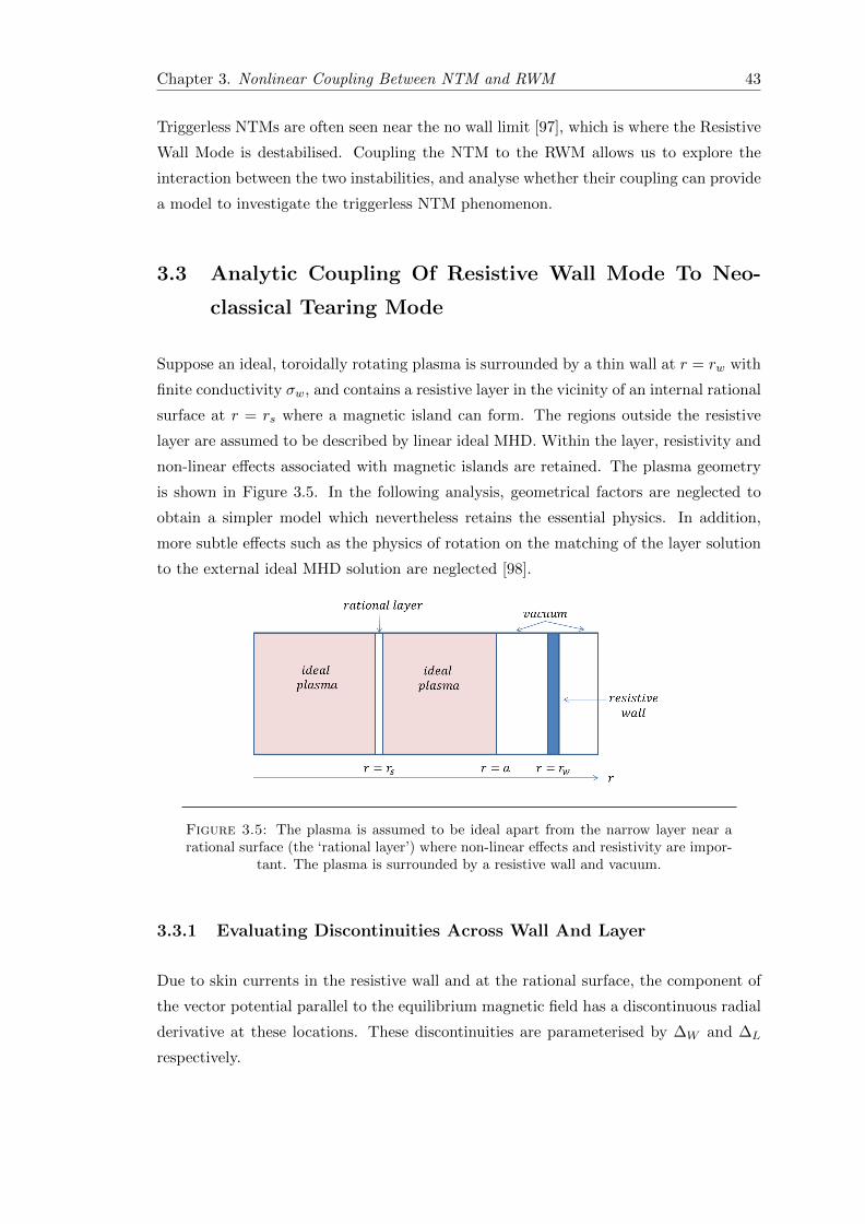
Chapter 3. Nonlinear Coupling Between NTM and RWM 43
Triggerless NTMs are often seen near the no wall limit [97], which is where the Resistive
Wall Mode is destabilised. Coupling the NTM to the RWM allows us to explore the
interaction between the two instabilities, and analyse whether their coupling can provide
a model to investigate the triggerless NTM phenomenon.
3.3 Analytic Coupling Of Resistive Wall Mode To Neo-
classical Tearing Mode
Suppose an ideal, toroidally rotating plasma is surrounded by a thin wall at r = rw with
finite conductivity σw, and contains a resistive layer in the vicinity of an internal rational
surface at r = rs where a magnetic island can form. The regions outside the resistive
layer are assumed to be described by linear ideal MHD. Within the layer, resistivity and
non-linear effects associated with magnetic islands are retained. The plasma geometry
is shown in Figure 3.5. In the following analysis, geometrical factors are neglected to
obtain a simpler model which nevertheless retains the essential physics. In addition,
more subtle effects such as the physics of rotation on the matching of the layer solution
to the external ideal MHD solution are neglected [98].
Figure 3.5: The plasma is assumed to be ideal apart from the narrow layer near arational surface (the ‘rational layer’) where non-linear effects and resistivity are impor-
tant. The plasma is surrounded by a resistive wall and vacuum.
3.3.1 Evaluating Discontinuities Across Wall And Layer
Due to skin currents in the resistive wall and at the rational surface, the component of
the vector potential parallel to the equilibrium magnetic field has a discontinuous radial
derivative at these locations. These discontinuities are parameterised by ∆W and ∆L
respectively.
Chapter 3. Nonlinear Coupling Between NTM and RWM 44
In a linear, ideal MHD cylindrical model using a complex representation of the perturbed
fields, ∆W and ∆L can be related in a simple way[35, 99]. This is because the MHD
eigenfunction in this situation is a second order differential equation [55].
∆L =1− δ∆W
−ε+ ∆W(3.4)
ε and δ depend on the equilibrium, and are related to the stability properties of the
plasma in the limit of no wall and a superconducting wall respectively. They can be
derived for a given equilibrium by solving ideal MHD equations outside the wall and
rational layer with appropriate boundary conditions at r = 0 and r = ∞, with the
(dimensionless) definition
∆L,W =rs,wψc
∂ψc∂r
∣∣∣∣r+s,wr−s,w
(3.5)
Here, ψc is the complex representation of the magnetic flux function derived from linear
ideal MHD. When no wall is present, ∆W = 0 and for an ideally unstable plasma (where
an inertial response for the layer is appropriate and ∆L < 0 corresponds to instability
to ideal MHD modes), ε is positive and small. For an ideal superconducting wall at
r = rw, ∆W → ∞ and δ > 0 provides stability to the internal kink mode, i.e. ∆L < 0.
Thus, equilibria with small ε, δ > 0 are susceptible to a RWM but avoid the internal
kink mode.
Whilst linear equations are solved in the outer region of the plasma, the need to an-
ticipate matching to the non-linear solution at the rational layer can be anticipated.
Assuming that the time dependence can be separated from the spatial dependence, the
outer region solution can be expressed
ψc(r, t) = ψeiξe∫ρdt (3.6)
where ρ(t) = γ(t)− iω(t), with γ the instantaneous growth rate, ω the mode frequency
relative to the wall, and ξ = mθ − nφ the helical angle defined in terms of the poloidal
(θ) and toroidal (φ) angles. It will be assumed that the toroidal mode number n = 1,
with m the poloidal mode number.
Resistive Wall Response
Using Ampere’s law in the thin resistive wall [100], the wall response can be calculated.

Chapter 3. Nonlinear Coupling Between NTM and RWM 45
For Faraday’s and Ohm’s Laws,
∂B
∂t= −∇×E = −∇× ηwJ (3.7)
where ηw = 1/σw is the wall resistivity (taken as a constant). Ampere’s Law implies
that
∇×∇×B = µ0∇× J (3.8)
Thus∂B
∂t=ηwµ0
(∇(∇ ·B)−∇2B) (3.9)
and it follows that, since ∇ ·B = 0,
∂B
∂t= −ηw
µ0∇2B (3.10)
Defining the complex magnetic flux function ψc as Br = − 1R∂ψc∂Z and BZ = 1
R∂ψc∂R , and
taking the radial component of Equation 3.10, we obtain
ηwµ0∇2ψc =
∂ψc∂t
(3.11)
Since the wall is assumed to be thin, ∇2 ∼ ∂2/∂r2.
∂2ψc∂r2
= µ0σw∂ψc∂t
(3.12)
Now consider the form of ψc, the complex magnetic flux function given in 3.6:
1
ψc
∂ψc∂t
= ρ (3.13)
Integrating across the thin wall and recalling the definition of ∆W given in 3.5, it is
possible to obtain
∆W = ρτ (3.14)

Chapter 3. Nonlinear Coupling Between NTM and RWM 46
where τ = τwτr
, and τw = µ0dσwrw is the wall diffusion time, with the wall thickness
d << rw, the minor radius at which the wall is located. The instantaneous complex
growth rate ρ is normalised to τr = σµ0ars, the resistive plasma diffusion time where σ
is the plasma conductivity at the rational surface. Combining these results, the linear
cylindrical dispersion relation [35] is obtained
∆L =1− δρτ−ε+ ρτ
(3.15)
3.3.2 NTM Evolution
In the linearised ideal MHD region of the plasma, a complex representation for the
magnetic flux is required to ensure that 3.4 holds [55]. The physical flux is denoted
ψL = Re[ψc]. In the rational layer where non-linear physics is retained, the complex
representation cannot be used, so the physical flux ψL is employed.
Assume a magnetic island exists at the rational surface. Transforming into the frame of
reference where the rational surface is at rest, the wall is rotating. Analogously to the
wall response, Ampere’s law describes the current perturbations at the rational surface
∂2ψL∂r2
= −µ0J|| (3.16)
where J|| is the component of current density perturbation parallel to the magnetic field.
There are two contributions to J|| considered: an inductive component proportional
to ∂ψL/∂t, and the perturbation in the bootstrap current Jbs caused by the pressure
flattening inside the island. For the induced current contribution, E|| can be expressed
as, firstly,
E|| = −∂A||
∂t(3.17)
due to the equivalences of
∂B
∂t=
∂
∂t(∇×A) = ∇× ∂A
∂t= −∇×E (3.18)
Then we consider that A|| is equal to ψL. Thus, J induced|| = σE|| = −σ ∂ψL∂t .
Assuming these current perturbations are localised within the layer, and integrating
across the layer, we obtain

Chapter 3. Nonlinear Coupling Between NTM and RWM 47
∂ψL∂r
∣∣∣∣r+sr−s
= 2σµ0w∂ψL∂t− 2µ0wJbs (3.19)
where w is the half-width of the magnetic island. The discontinuity on the left hand
side of 3.19, caused by the current sheet in the layer, can now be expressed in terms of
∆L.
ψL is assumed to be of the form ψL = ϕ cos(α + ζ), where α = ξ −∫ωdt, ζ(r) is a
phase factor. The mode frequency in this rotating frame is ω = ω − ΩL, where ΩL is
the toroidal plasma rotation frequency at r = rs relative to the stationary wall.
Evaluating ∂ψL∂r
∣∣∣∣r+sr−s
The left hand side of 3.19 is evaluated by matching to the ideal MHD solution in the
outer regions of the plasma.
The complex representation of the magnetic flux function 3.6 can be decomposed into
its real and imaginary parts:
Re[ψc] = e∫γdt(Re[ψ] cos α− Im[ψ] sin α) (3.20)
Im[ψc] = e∫γdt(Re[ψ] sin α+ Im[ψ cos α]) (3.21)
recalling that ψ is the amplitude of the magnetic flux function in 3.6.
If ψL = ϕ cos(α+ ζ), then
ψL = ϕ(cos α cos ζ − sin α sin ζ) (3.22)
Hence, if Re[ψc] = ψL, the coefficients of cos α and sin α can be matched between 3.20
and 3.22
Re[ψ]e∫γdt = ϕ cos ζ (3.23)
Im[ψ]e∫γdt = ϕ sin ζ (3.24)
Now, since ∆L is defined in terms of ψc,

Chapter 3. Nonlinear Coupling Between NTM and RWM 48
∂ψL∂r
∣∣∣∣r+sr−s
=1
rs(Re[∆L]Re[ψc]− Im[∆L]Im[ψc]) (3.25)
Substituting for Re[ψc] and Im[ψc] using 3.20, 3.21, and then using 3.23, 3.24
∂ψL∂r
∣∣∣∣r+sr−s
=ϕ
rs(Re[∆L] cos(α+ ζ)− Im[∆L] sin(α+ ζ)) (3.26)
Nonlinear Island Effects
Combining 3.26 with 3.19, and taking the time derivative of ψL yields
ϕ
rs(Re[∆L] cos(α+ζ)−Im[∆L] sin(α+ζ)) = 2σµ0w
(∂ϕ
∂tcos(α+ζ)+ωϕ sin(α+ζ)
)−2µ0wJbs
(3.27)
Multiplying by cos(α+ ζ) or sin(α+ ζ), and the integrating over α yields equations for
w and ∂ϕ/∂t. The island half-width w is related to ϕ by [3]:
w2 =4rsLsϕ
BθqR(3.28)
where Ls = Rq/s is the shear length scale, q is the safety factor, s is the magnetic shear,
R is the major radius, and Bθ is the poloidal magnetic field. Normalising the island
half-width to the minor radius a, and time t to τr, we obtain two equations
4w = Re[∆L] + βw
(1− w2
cw2
)(3.29)
2w(ω − ΩL) + Im[∆L] = 0 (3.30)
where w refers to time derivatives of w with respect to t = t/τr, and Jbs = (βθBθ√ε/Lpµ0) cos(α+
ζ), where βθ is the poloidal beta, ε the inverse aspect ratio, 1/Lp = (1/p)(dp/dr) the
pressure length scale and wc the seed island threshold width. This results in a definition
of β = (8√εβθrs/Lps).
It is important to note that γ = 2w/w, ω and ΩL have been normalised to τr also.
In addition to the bootstrap current Jbs, a heuristic threshold term (1 − w2c/w
2) has
been added. This introduces the essential non-linear seed island physics needed for

Chapter 3. Nonlinear Coupling Between NTM and RWM 49
studying the NTM. As discussed briefly above, the threshold term can be attributed to
the polarisation current effects [83].
Equation 4.1 is the same relation as found in [101] if the plasma toroidal rotation is not
considered. The full expression for ∆L in terms of γ, ω and ΩL is given by
∆L =(1− δτγ)(ε+ τγ)− δτ2ω2
(−ε+ τγ)2 + τ2ω2+ i
τω(1− εδ)(−ε+ τγ)2 + τ2ω2
(3.31)
3.4 Toroidal Torque Balance
The plasma toroidal rotation at the rational surface, ΩL, has so far not been dealt with.
In order to determine ΩL self-consistently, the torque balance in the plasma must be
calculated. Ideal plasma is torque-free [102], and so the torque exerted on the plasma is
a delta-function at the rational surface, δ(r − rs).
Consider the perturbed MHD momentum balance equation in the non-ideal layer, aver-
aged over the flux surface
〈δJ× δB〉+ ρµ∇2v = 0 (3.32)
where the angled brackets denote the average over a flux surface. Here ρ is the plasma
density and µ the plasma viscosity. It can be assumed that the processes under consid-
eration occur over many viscous diffusion times, and pressure is constant across the thin
layer. The pressure gradient is neglected as it will not contribute once 3.32 is integrated
across the layer (as follows).
Assume that v is continuous across the layer, but ∇v possesses a discontinuity at r = rs
due to the localised torque at that location. For a perturbation δB, ∇×δB = −∇2ψLb.
Only the toroidal component is required. Integrating 3.32 over the rational layer
⟨ϕ
Rµ0sin(α+ ζ)
∂ψL∂r
∣∣∣∣r+sr−s
⟩+ ρµ
∂vφ∂r
∣∣∣∣r+sr−s
= 0 (3.33)
The discontinuity in the radial derivative of ψL = Re[ψc] is evaluated as before. Inte-
grating over α, all terms containing Re[∆L] disappear.
If vφ = ΩR, then using the normalisations described above,
∂Ω
∂r
∣∣∣∣r+sr−s
=A
aw4Im[∆L] (3.34)

Chapter 3. Nonlinear Coupling Between NTM and RWM 50
such that A = s2ε2a3τvτr/512r3sq
2τ2A, with τv = a2/µ the momentum confinement time,
a the minor radius, and τA = (a√
(µ0ρ)/B) the Alfven time, and taking σ = T3/2e /1.65×
10−9 lnλ, with Te expressed in keV. The safety factor q at r = rs will be taken as q = 2.
The electromagnetic torque is finite when Im[∆L] 6= 0, and always acts to damp the
plasma rotation [56]. Im[∆L] is related to the discontinuity in the derivative of the phase
factor ζ [35]: the torque only acts on the plasma in the rational layer when ∂ζ∂r |
r+sr−s6= 0.
In the outer ideal plasma, the momentum equation is simply
d2Ω
dr2= 0 (3.35)
The linear rotation profile in the ideal plasma regions r < rs and rs < r < a is continuous
at r = rs, but has a discontinuity in the first radial derivative there, caused by the torque.
Imposing no-slip boundary conditions at the outer edge of the plasma r = a (viscous
drag effects) and a driving force at the inner edge at r = 0 that maintains dΩdr = −Ω0/a,
the toroidal rotation frequency profile can be constructed in the region of ideal plasma.
Ω(r) =
λ(a− rs) + Ω0
a (rs − r) 0 < r < rs
λ(a− r) rs < r < a
for constant λ > 0. The discontinuity in the radial derivative is calculated to be
−λ + Ω0/a. Hence, at r = rs, using 3.34, the damping of the toroidal plasma rota-
tion frequency is found to be given by
(Ω0 − fΩL) = Aw4Im[∆L] (3.36)
where f = a/(a− rs).
Appendix B describes the similar model constructed by Gimblett and Hastie in [55], and
its difference from this approach.
3.5 Summary Of Results
The theory of classical and neoclassical tearing modes was discussed, with particular
emphasis on the threshold properties of both the island width and the value of βθ. In
addition, the phenomenon of triggerless NTMs is introduced. A system where an NTM
is coupled to a RWM is derived. By coupling together the resistive wall and the rational
layer where the magnetic island is located (and the respective discontinuities in the
Chapter 3. Nonlinear Coupling Between NTM and RWM 51
magnetic flux function); and including a self consistent evaluation of the torque at the
rational surface, a non-linear system of equations can be found.
Chapter 4
Solutions For Coupled
NTM-RWM In A Rotating
Plasma
In the previous chapter, the derivation of a system of non-linear equations which de-
scribes the evolution of a coupled NTM-RWM system was explained. The first step
was to establish the coupling mechanism between the two modes- the link is provided
by the respective parameters, ∆L,W , for the rational layer where the magnetic island
is located, and the resistive wall surrounding the plasma. The island evolution in the
rational layer was evaluated, with the contribution from the bootstrap current of partic-
ular importance. To close the system, the torque at the rational layer is also determined
self-consistently. The resultant equations are shown below
4w = Re[∆L] + βw
(1− w2
cw2
)(4.1)
2w(ω − ΩL) + Im[∆L] = 0 (4.2)
(Ω0 − fΩL) = Aw4Im[∆L] (4.3)
where ∆L is a complex function of γ and ω.
For the following analysis, τ ∼ 10−2, corresponding to a choice of a = 1.0m, rs = 0.5m,
Te = 1keV, and Coulomb logarithm lnλ = 20. The equilibrium parameters will be taken
as ε = 0.1, and δ = 5, unless otherwise indicated.
52

Chapter 4. Solutions For Coupled NTM-RWM System 53
4.1 No Wall Solution
If there is no wall surrounding the plasma, then this implies that τ = 0. In this situation,
the RWM is not a solution of the system- instead, an infinite growth rate is obtained as
a solution, which can be interpreted as the ideal kink mode.
However, the NTM is still a solution in this limit, as shown in Figure 4.1. The NTM
solutions exhibit the important threshold characteristics which are fundamental to the
NTM, as described in Section 3.1.2. For a β below a critical value, dw/dt < 0 ∀w, and
so all islands will decay - and thus no islands exist in the plasma. For β greater than the
critical value, there are two solutions for dw/dt = 0. These are the equilibrium points
for the system. The first equilibrium point is unstable, in that any perturbations from
this point cause the island either to shrink or to grow larger (away from the equilibrium
point). This equilibrium point is a threshold for the island growth. The size of the island
at this equilibrium point will be referred to as the seed island width or the critical island
island. For an island larger than this threshold width, the island will grow because
dw/dt > 0. It will continue to grow until it reaches the second equilibrium point, which
is stable. This corresponds to a large, saturated NTM.
When τ is finite, both RWM and NTM branches are present. If the wall is thin, or has
low conductivity, then it can be assumed that τ << 1 and the equations can be solved
analytically.
4.2 Limiting Solution For Small Islands
The behaviour of the solutions when the island is small, w << wc, can be considered
first. For a traditional NTM, an island of this size would not grow, as it is smaller
than the threshold width required for a seed island, as discussed above. Terms can be
ordered: τω << τγ ∼ ε in order to analyse the small island limit.
The bootstrap term in Equation 4.1, which is ∼ β, is relatively large at w < wc, and
negative. This term must then be balanced by either a large w (ie, γ) on the left hand
side of Equation 4.1, or by a large value of Re[∆L].
Neglecting τω in Equation 4.1, the solution branch when γ is large and negative is the
stable NTM root of the equations- as shown in Figure 4.1. Specifically, in this limit,
Re[∆L] ∼ δ and γ < 0 for w < wc.

Chapter 4. Solutions For Coupled NTM-RWM System 54
Figure 4.1: No RWM exists when the resistive wall is removed: only the NTMsolution. The dependence of the island width evolution on β and w illustrates the
behaviour expected for a NTM. This is same behaviour as seen in Section 3.1.2.
Chapter 4. Solutions For Coupled NTM-RWM System 55
The alternative is the RWM solution branch, in which the denominator of Re[∆L] is
small. Neglecting the left hand side of Equation 4.1, and balancing Re[∆L] against the
bootstrap term, yields a RWM which grows at the rate
τγ = ε− w
β
(1− w2
c
w2
)−1
(4.4)
Thus, an island such that w < wc will have γ > 0 and will grow steadily despite being
below the NTM threshold width.
When w approaches wc, the growth rate is substantially enhanced by the coupling to
the bootstrap term. Indeed, as w → wc, τγ →∞, but this is unphysical. The ordering
breaks down.
Similarly, with the assumptions that ω << ΩL and τω << 1, the RWM frequency and
toroidal rotation frequency can be found.
τω = 2w3Ω0
(1−εδ)β2
(w2c
w2 − 1
)−2
(f + 2Aw5)−1 (4.5)
ΩL = Ω0f+2Aw5 (4.6)
Equation 4.6 shows that the plasma rotation at the rational surface, ΩL, decreases
steadily in time from its initial value of Ω0/f as the island grows. The mode is initially
locked to the wall (τω = 0 when w = 0), but as the island grows, the mode frequency
ω gradually increases. Nevertheless, it remains very small, much less than ΩL. This is
a consequence of Equation 4.4, which implies that Im[∆L] is very large. Since Im[∆L]
is directly proportional to the electromagnetic torque at the rational surface,, the elec-
tromagnetic torque at r = rs is very large. Hence there is no rotational stabilisation of
the RWM in Equation 4.4. This is different to the model presented in [99], where the
bootstrap term is not included. There, the RWM mode frequency rises faster with ΩL,
leading to a suppression of its growth rate as ΩL increases (the increased mode frequency
leads to a stabilising relative rotation between the wall and the mode).
It can be noted that ω is increasingly sensitive to the island width as w approaches wc.
This indicates an unlocking of the island and a dramatic spin-up. Again, as w → wc,
Equation 4.6 predicts τω →∞ and the assumed ordering is again broken.
In conclusion, for w < wc, a slowly growing mode which is locked to the wall is found.
This is the RWM solution branch. As the island width w approaches wc, there is a
Chapter 4. Solutions For Coupled NTM-RWM System 56
substantial increase in the growth of the island, and the mode begins to spin up. The
small τγ, small τω ordering fails. As τγ, τω grow, the full expansion of ∆L
∆L =(1− δτγ)(ε+ τγ)− δτ2ω2
(−ε+ τγ)2 + τ2ω2+ i
τω(1− εδ)(−ε+ τγ)2 + τ2ω2
(4.7)
implies that Im[∆L]→ 0. The electromagnetic torque which locks the mode to the wall
is reduced, and the mode will spin up to rotate with the plasma. Equation 4.3 then
indicates that this forces Ω0− fΩL ≈ 0, meaning that the plasma also spins up towards
the initial rotation frequency profile.
4.3 Numerical Solutions To Non-linear System
The non-linear system can be integrated numerically such that the island width w, the
mode frequency ω, and the toroidal rotation frequency at the rational surface ΩL are
functions of time. Since the island half width w is related to the mode growth rate by
γ = 2ww , the only variable with a time derivative in the non-linear system is w (there
is no ω term since inertia was neglected). Thus, the integration in time is carried out
on w only. At time step ti with the interval between time steps δt, the time integration
scheme is simply w(ti+1) = w(ti) + δt ∗ γ(ti).
Since the system is non-linear, it is solved numerically. The chosen method is by the
Newton-Raphson method. By rearranging the equations such that a vector function F
can be written as F(x), from an initial estimate of x0 = (t, w, ω,ΩL), an iteration of
the method will result in the accurate solution. The inverse Jacobian matrix J−1(x)
for F(x) is required, and the correction δx required at each iteration to improve the
estimate of x) is calculated by
J(x) · δx = −F(x) (4.8)
The initial guess for x needs to be chosen carefully for the Newton-Raphson method
to converge on the correct solution. This can be given by the limiting solution of the
system, which is described in detail in Section 4.2.
Figure 4.2 shows the comparison between the limiting analytical solutions (Equations
4.4, 4.6 and 4.6) to numerical solutions of the full system, given in Equations 4.1, 4.2
and 4.3. There is good agreement between the analytical and the numerical solutions
for small island widths, and then, as expected, the analytic theory fails. Nevertheless,

Chapter 4. Solutions For Coupled NTM-RWM System 57
Figure 4.2: The comparison of the analytic solutions valid for w < wc with thenumerical solutions of the full system: A and B show both τγ and τω increasingrapidly as w passes through wc. In C, the forced plasma spin-up observed in thenumerical solutions is not captured in the analytic approximation. Parameters are
fixed at Ω0 = 100, wc = 0.02 and β = 1.0.

Chapter 4. Solutions For Coupled NTM-RWM System 58
there is strong qualitative agreement, both approaches showing a stronger growth and
mode spin-up of the coupled RWM-NTM system as w passes through wc.
The dependence of the system behaviour on system parameters is also examined numer-
ically.
4.3.1 Dependence on β
If there is zero β, then the NTM has zero drive. In this case, the system finds a con-
ventional RWM as the solution. The mode rotates at a fraction of the plasma rotation,
but acting to slow the plasma. The mode eventually locks to the wall. Rotation is
expected to be stabilising in this situation [99]. This qualitative behaviour is shown in
Figure 4.3 for the lowest value of β: in this model, the RWM behaviour is prevalent for
a sufficiently small β.
At sufficiently large β, the RWM couples to a NTM, and takes on a different character.
Numerical solutions for a range of β values are shown in Figure 4.3. The seed island
is given a width wseed = wc/4, such that the NTM solution is stable. However, the
solutions show no threshold seed width for the coupled RWM-NTM mode: the mode
growth rate is positive for all island widths, however small. In Figure 4.3A, the seed
island grows steadily independent of β as expected for a ‘classic’ RWM, until it reaches
a width wc. This is consistent with the analytic solution in Equation 4.4, γ = ε/τ .
When w increases above wc, the island growth rate increases dramatically for high β as
the bootstrap term becomes destabilising, providing an additional drive for the mode.
This is not captured in the analytic results. If β is reduced, then the NTM drive
is reduced and its effect on the island growth is either reduced or insignificant. The
plasma rotation frequency at r = rs, ΩL, is damped by torque exerted by the unstable
RWM, until the island reaches wc, as shown in Figure 4.3D. The plasma then briefly
spins up as the RWM couples to the NTM drive, before again slowing to lock to the wall
at large w. Throughout the period for which w ≥ wc, the plasma and mode are locked-
the mode rotates with the plasma, which is a characteristic of NTMs.
The magnitude of the spin-up in plasma rotation is variable. It depends on the mag-
nitude of β. Since the NTM is driven by β, it is clear that increasing the NTM drive
affects the behaviour of the RWM branch. It is possible to remove the plasma spin-up
by decreasing β sufficiently - i.e. by removing drive for the NTM. This is consistent
with the picture that the NTM drive is the underlying physics. In Figure 4.3, it can
be observed that removing the NTM drive by reducing β causes the solution to behave

Chapter 4. Solutions For Coupled NTM-RWM System 59
Figure 4.3: The initial island, w(t = 0) = 0.005, which is considerably smaller thanthe critical seed island width wc = 0.02. The dependence of the island growth, growthrate γ, mode frequency and plasma rotation frequency at the rational surface on β isshown: increasing β increases the NTM drive and allows the island to grow faster and
to a larger size.
Chapter 4. Solutions For Coupled NTM-RWM System 60
more as a classic RWM. This would include features such as the wall locking of both the
mode and the plasma.
The transient spin-up is a particular feature of the coupled NTM-RWM mode which
would distinguish it from other interpretations of experimental observations. This spin-
up takes place over a time scale of 3-4 milliseconds for the chosen parameters, which
would be detectable: but the effects of including the plasma inertia (which has been ne-
glected in the formulation of the non-linear equations) may be important in determining
this time scale. Thus it may be that the actual time scale is rather different.
4.3.2 Dependence on Ω0
The island evolution is also influenced by the amount of momentum injected into the
plasma core, described here by the parameter Ω0. The effects of the variation of Ω0 is
shown in Figure 4.4.
It is important to note that in this model, the RWM is not sensitive to the plasma
rotation, as evidenced by the independence from Ω0 of the initial evolution of the island
width, until w = wc. This is consistent with the analytic solution in Equation 4.4, but
differs from models that do not include the NTM drive [99].
The coupling to the NTM is strongly influenced by torque, however. The dramatic
increase of island growth rates for w > wc is only observed at the lowest Ω0. At higher
Ω0 the mode evolves as a classic RWM which is locked to the wall, with a substantially
reduced growth rate compared to the low Ω0 cases when w > wc.
4.3.3 Equilibrium Parameters
The equilibrium parameters ε and δ are determined by the equilibrium of the plasma.
They are determined by the outer, ideal MHD region of the plasma. For an equilibrium
which is unstable to the RWM but avoids the internal kink, small ε and δ > 0 are chosen.
If the value of ε is changed, then the stability of the equilibrium to the RWM is altered.
Figure 4.5 shows that if ε is increased to ε = 0.3, then the NTM drive is not coupled to
the initial RWM-driven growth of the mode. The island saturates at the NTM threshold
width wc, and the plasma locks to the wall.
If the equilibrium is altered to be stable to ideal modes (ε = −0.1), then as expected
the initial island shrinks, and is no longer a solution, demonstrated in Figure 4.6. This
is because the unstable RWM is no longer present, and cannot drive the island growth.

Chapter 4. Solutions For Coupled NTM-RWM System 61
Figure 4.4: Initially, w(t = 0) = 0.005, and β = 1.0. A demonstrates that the initialplasma rotation frequency has a noticeable effect on the island evolution, whereas Band C contrast the mode growth rates and mode frequencies for differing values ofΩ0. D, E and F show the mode and rotation frequencies for the same values of Ω0.Ω0 = 104 corresponds to the plasma rotating at about 5 % of the plasma sound speed.
The spin-up of the plasma only occurs for very small plasma rotation frequencies.

Chapter 4. Solutions For Coupled NTM-RWM System 62
Since the island is below the NTM threshold width, the NTM drive is also inaccessible.
The rotation frequency remains unchanged from its initial value, and the mode is locked
to the wall.
The parameter δ can also be altered to change the plasma stability when it is surrounded
by an ideal wall at r = rw. The results are shown in Figure 4.7. According to Equation
4.4, δ doesn’t alter the island behaviour for w < wc, which can be clearly seen in Figure
4.7. The qualitative behaviour of the system for w > wc is similar, but the change in
δ alters the time of onset of the increased growth rate and plasma spin-up. The island
grows to its largest size when δ = −5.0, which corresponds to instability to internal kink
modes (∆L < 0).
4.4 Summary of conclusions
The system of equations 4.1, 4.2 and 4.3 have two solution branches: a NTM with the
characteristic thresholds in β and seed island width; and a coupled RWM-NTM branch
which has no threshold.
Whilst the RWM-NTM island width is small, below the NTM threshold width, the
mode is a ‘classic’ RWM. The mode grows slowly on a timescale characterised by the
wall resistive diffusion time, and is locked to the wall. The plasma rotation gradually
slows during this phase.
As the island width exceeds the NTM threshold width, there is a dramatic increase in
growth as the mode couples to the NTM drive. This is particularly noticeable at high β.
At the same time, the mode unlocks from the wall and instead rotates with the plasma.
The plasma rotation increases at this time. The island continues to grow, locked to the
plasma flow, which gradually slows to lock to the wall at large island width, This phase
has the characteristics of an NTM.
4.4.1 Experimental Observations
In order to be a worthwhile model, the behaviour predicted here should be experimen-
tally testable, as well as distinguishable from other models. Only tokamaks which have
a resistive wall and which are capable of demonstrating a resistive wall mode would be
able to test this model - for example, the design of spherical tokamaks places the wall
sufficiently far from the plasma as to be at infinity. Tokamaks such as DIII-D (Figure
2.8) and JT-60U (Figure 2.9) are capable of analysing RWM behaviour, and DIII-D

Chapter 4. Solutions For Coupled NTM-RWM System 63
Figure 4.5: Comparison of ε = 0.1 and ε = 0.3 for Ω0 = 100 and β = 1.0. Changingthe equilibrium stability to the RWM changes the island behaviour.
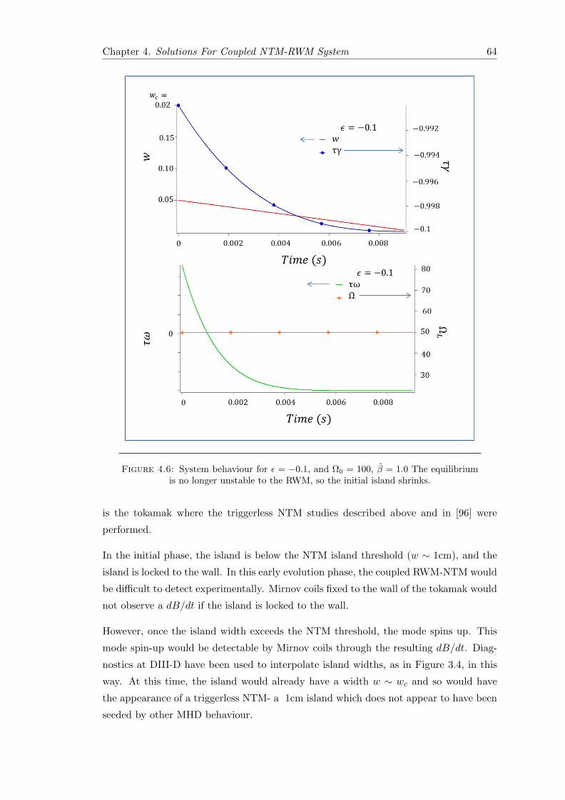
Chapter 4. Solutions For Coupled NTM-RWM System 64
Figure 4.6: System behaviour for ε = −0.1, and Ω0 = 100, β = 1.0 The equilibriumis no longer unstable to the RWM, so the initial island shrinks.
is the tokamak where the triggerless NTM studies described above and in [96] were
performed.
In the initial phase, the island is below the NTM island threshold (w ∼ 1cm), and the
island is locked to the wall. In this early evolution phase, the coupled RWM-NTM would
be difficult to detect experimentally. Mirnov coils fixed to the wall of the tokamak would
not observe a dB/dt if the island is locked to the wall.
However, once the island width exceeds the NTM threshold, the mode spins up. This
mode spin-up would be detectable by Mirnov coils through the resulting dB/dt. Diag-
nostics at DIII-D have been used to interpolate island widths, as in Figure 3.4, in this
way. At this time, the island would already have a width w ∼ wc and so would have
the appearance of a triggerless NTM- a 1cm island which does not appear to have been
seeded by other MHD behaviour.

Chapter 4. Solutions For Coupled NTM-RWM System 65
Figure 4.7: Scan of differing values of δ for Ω0 = 100 and β = 1.0. Qualitativebehaviour is unvaried but the onset of the NTM-like phase occurs at slightly different
times.
Chapter 4. Solutions For Coupled NTM-RWM System 66
One advantage of testing this model at DIII-D would be that existing experimental
protocols and expertise for studying triggerless NTMs would be already in place, which
would enable the difference between the model described in this thesis, and the model
described in [96], to be compared effectively. The plasma βN would increase towards the
no-wall limit, as in [96], avoiding destabilising sawtooth activity. This model predicts
that the destabilised RWM would drive island growth until the island width w ∼ wc,
when the neoclassical bootstrap current would begin to drive the island until saturation.
Observations of the island unlocking and subsequent locking would need to be combined
with detailed analysis of plasma rotation at the rational surface: although the plasma
spin-up may be too fast to be detected, since this model neglects plasma inertia. Control
of the plasma rotation in a sequence of experiments would also be beneficial in order to
capture any plasma spin-up behaviour.
4.4.2 Contrasting Interpretations Of Triggerless NTMs
The phenomenon of triggerless NTMs near βno−wallN , the ideal no-wall βN limit, can also
be explained by using the concept of ∆′. In particular, the behaviour of ∆
′near the
no-wall limit, where ∆′
is implemented here as ∆L/rs.
As βN → βno−wallN , then ∆′ →∞ (∆W = 0 since there is no wall, and ε→ 0). This can
cause an NTM to grow, either because a classical tearing mode is destabilised, which
in turn destabilises the neoclassical tearing mode when at sufficiently large amplitude;
or the threshold island width is lowered for non-linear NTM destabilisation, so that
smaller seed islands produced by forced magnetic reconnection at the rational surface
caused by other modes are able to grow [96]. This is because the growth rate of the
mode becomes very sensitive to equilibrium parameters when ∆′
becomes large, leading
to rapid changes in mode stability [103].
In the model derived in this thesis, this would be equivalent to allowing ∆w → 0 and
ε → 0, corresponding to the no-wall ideal MHD stability boundary. The RWM is
destabilised for βN > βno−wallN , but the pole in ∆L is resolved by a dependence on the
wall response. The physics interpretation is thus somewhat different to that given in
[96]. A distinguishing prediction is that, contrary to the model dependent on a pole
in ∆′, the plasma is expected to slow in the few tens of milliseconds before the island
width reaches the threshold width. Additionally, the plasma spin-up coincident with the
appearance of the mode on Mirnov coils, would manifest and last a few milliseconds.
However, if the plasma rotation is sufficiently fast, the characteristic mode spin-up does
not occur (Figure 4.4F).

Chapter 4. Solutions For Coupled NTM-RWM System 67
4.5 Summary Of Results
The system of non-linear equations found in Chapter 3 is solved for a variety of situations.
For a plasma surrounded by no wall, the NTM is found as a solution, and exhibits the
typical threshold physics expected of an NTM. If the magnetic island width is small,
the equations can be solved analytically. This provides an initial guess for solving the
system of equations numerically. In varying system parameters, the behaviour of the
coupled mode is seen to be similar to that of a triggerless NTM. Thus, a RWM coupled
to an NTM is a possible explanation for observations of triggerless NTMs in tokamak
experiments.
Chapter 5
Benchmarking Resistive Walls in
JOREK
5.1 Nonlinear MHD Simulations With JOREK
JOREK is a nonlinear code which solves the reduced MHD equations in toroidal ge-
ometry. It was developed by G. T. A. Huysmans [104] and originally intended to aid
the understanding of ELMs [105, 106]. In the poloidal plane, third order Bezier finite
elements are used as the spatial discretisation [107], whereas in the toroidal direction a
Fourier decomposition is employed. Thus a 3D model of the plasma can be simulated.
The code is OpenMP and MPI parallelised. The libraries needed include PASTIX [108],
Scotch [109] and MUMPS [110].
5.1.1 JOREK Equilibrium
JOREK incorporates the HELENA equilibrium solver [111]. The code requires primar-
ily the density, temperature and FF ′ profiles (where F = RBφ [3]) and the plasma
geometry as inputs. In addition to minor and major radii, the computational boundary
is defined by either (R,Z,Ψ) coordinates (Ψ is poloidal flux) or ellipticity, triangularities
and quadrangularities.
After initialisation, JOREK defines the computational boundary and the initial grid for
solving the equilibrium. JOREK then solves the Grad-Shafranov equation in weak form.
The weak form of Equation 5.1 is found my multiplying 5.1 by a test function (usually a
basis function to simplify integration) and integrated over the calculation domain. This
technique allows for higher order derivatives to be reduced by integration by parts, such
68

Chapter 5. Benchmarking JOREK 69
that the equation to be solved does not include any derivative of the function that is
being solved for. This allows solutions which may not be smooth to be found.
R∂
∂R
(1
R
∂Ψ
∂R
)+∂2ψ
∂Z2= −R2 ∂p
∂Ψ− F ∂F
∂Ψ(5.1)
where (R,Z) are coordinates in the poloidal plane and p is pressure.
When the flux surfaces have been calculated, the grid is adjusted to align with the flux
surfaces.
5.1.2 Reduced MHD Equations
JOREK evolves the equilibrium in time, solving the reduced MHD equations. The
reduced MHD equations are as follows:
• Poloidal Flux Equation,
1
R2
∂Ψ
∂t= η(T )∇ ·
(1
R2∇⊥Ψ
)=
1
R[u,Ψ]− F0
R2
∂u
∂φ
• Poloidal Momentum Equation,
eφ · ∇ ×(ρ∂v
∂t= −ρ(v · ∇)v −∇(ρT ) + J×B + µ∆v
)• Toroidal Current Equation,
j = ∆∗Ψ
• Vorticity Equation,
ω = ∇2⊥u
• Density Equation,
∂ρ
∂t= −∇ · (ρv) +∇ · (D⊥∇⊥ρ) + Sp
• Temperature Equation
ρ∂T
∂t= −ρv · ∇T − (κ− 1)ρT∇ · v +∇ · (K⊥∇⊥T +K‖∇‖T ) + ST

Chapter 5. Benchmarking JOREK 70
• Parallel Momentum (only if selected by choice of JOREK model)
B ·
(ρ∂v
∂t= −ρ(v · ∇)v −∇ρ+ J×B + µ∆v
)
where η is plasma resistivity, T is plasma temperature, u is the stream function, v is
velocity, ρ is density, J is current density, B is magnetic field, ∆∗ = R2∆ · (R−2∇), j
is toroidal current density, ω is vorticity, Sρ is a density source, κ the ratio of specific
heats, and ST is a temperature source. K is the transport coefficient, and D is particle
diffusivity.
The magnetic field is defined as
B =F0
Reφ +
1
R∇Ψ× eφ
and the flow as
v = −R∇u× eφ + v‖B
The weak form of each equation is calculated: as with Equation 5.1, test functions
equivalent to the JOREK basis functions - Bezier and Fourier basis functions [112]-
are chosen, and any higher derivatives can be reduced by partial integration. The
physical quantities are also expanded in the basis functions. Integrals are carried out
by Gauss quadrature in element-local coordinates in the poloidal plane and by Fast
Fourier Transform toroidally. This results in a linear system of equations, which can be
represented as a large sparse matrix. The time stepping is a Crank-Nicholson scheme.
5.2 Coupling JOREK And STARWALL
The default boundary conditions for simulations using JOREK are fixed: the JOREK
computational domain is surrounded by an ideally conducting wall. In the equations
solved by JOREK, the only place the boundary response is invoked is in the current
equation. Fixed boundary conditions cause the integral around the boundary in the
current equation to disappear. When implementing the free boundary conditions, this
boundary integral remains finite.

Chapter 5. Benchmarking JOREK 71
5.2.1 STARWALL
The STARWALL code [113] solves the magnetic field equation in a vacuum (as a
Neumann-like problem). The code can do this in the presence of 3D conducting struc-
tures (generally referred to collectively as the “wall”) which can include holes, coils and
other 3D structures. This allows the inclusion of realistic wall geometry, and modelling
MHD stability in machine-specific configurations.
The wall is modelled as infinitely thin triangles with the wall current potentials assumed
to be constant over each wall triangle. The wall is also characterised by its effective
resistance ηw/dw where ηw is the wall resistivity (JOREK-normalised) and dw the wall
thickness. Since the wall current potentials are assumed to be constant over a wall
triangle, they can be described by the wall current potentials Yk on the triangle nodes.
STARWALL has also been coupled to the CASTOR MHD code to perform linear sta-
bility studies with a resistive wall [114].
5.2.2 Boundary Conditions
In the coupling of STARWALL to JOREK, the boundary condition is given by the
component of the magnetic field normal to the boundary of the JOREK computational
domain in the poloidal plane. This boundary is often referred to as the interface [115].
STARWALL generates response matrices for the specified 3D wall structure which can
be used to express the magnetic field component tangential to the interface in terms of
the normal component.
5.2.3 Implementing The Boundary Integral
The implementation of the boundary integral in JOREK was carried out by M. Holzl.
The vacuum response provided by STARWALL is needed only when implementing the
current equation
j = ∆∗Ψ (5.2)
where the operator ∆∗ = R2∇ · (R−2∇). The equations are written in weak form,
with the basis functions acting as the test functions j∗. These basis functions are the
1D Bezier basis function in the poloidal direction on the interface, or the Fourier basis
function in the toroidal direction. From the weak form (Equation 5.3) of the current
equation,
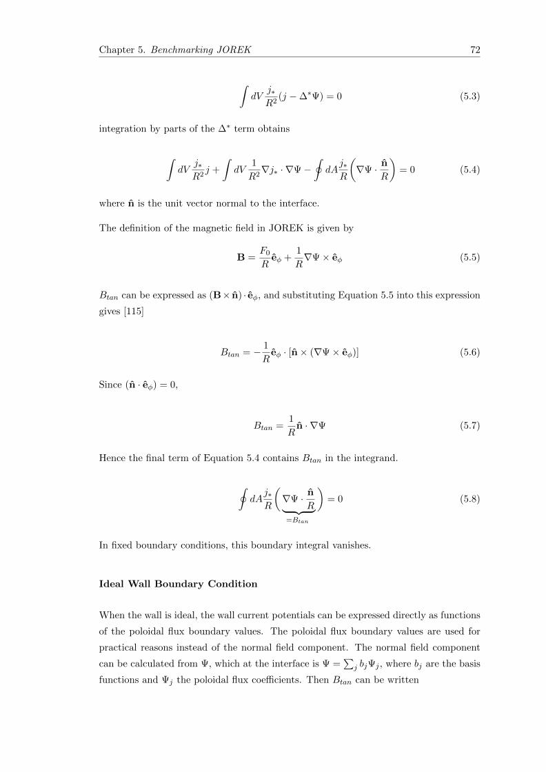
Chapter 5. Benchmarking JOREK 72
∫dV
j∗R2
(j −∆∗Ψ) = 0 (5.3)
integration by parts of the ∆∗ term obtains
∫dV
j∗R2
j +
∫dV
1
R2∇j∗ · ∇Ψ−
∮dA
j∗R
(∇Ψ · n
R
)= 0 (5.4)
where n is the unit vector normal to the interface.
The definition of the magnetic field in JOREK is given by
B =F0
Reφ +
1
R∇Ψ× eφ (5.5)
Btan can be expressed as (B× n) · eφ, and substituting Equation 5.5 into this expression
gives [115]
Btan = − 1
Reφ · [n× (∇Ψ× eφ)] (5.6)
Since (n · eφ) = 0,
Btan =1
Rn · ∇Ψ (5.7)
Hence the final term of Equation 5.4 contains Btan in the integrand.
∮dA
j∗R
(∇Ψ · n
R︸ ︷︷ ︸=Btan
)= 0 (5.8)
In fixed boundary conditions, this boundary integral vanishes.
Ideal Wall Boundary Condition
When the wall is ideal, the wall current potentials can be expressed directly as functions
of the poloidal flux boundary values. The poloidal flux boundary values are used for
practical reasons instead of the normal field component. The normal field component
can be calculated from Ψ, which at the interface is Ψ =∑
j bjΨj , where bj are the basis
functions and Ψj the poloidal flux coefficients. Then Btan can be written
Chapter 5. Benchmarking JOREK 73
Btan =∑i
biBtan,i =∑i
bi∑j
M idi,jΨi (5.9)
with M id the STARWALL-calculated ideal wall response matrix. The wall current po-
tentials Yk are not considered explicitly.
Resistive Wall Boundary Condition
For a resistive wall, the wall current potentials are considered.
Btan =∑i
bi
(∑j
M eei,jΨj +
∑k
M eyi,kYk
)(5.10)
M ee and M ey are the STARWALL resistive response matrices. The wall current poten-
tials also evolve in time,
Yk = −ηwdwMyyk,kYk −
∑j
M eyi,kΨj (5.11)
with Myy and M ey also STARWALL matrices.
By taking ηw → 0, it is clear that M idi,j ≡ M ee
i,j −∑
k Meyi,kM
yek,j . Similarly, by letting
Yk → 0, the no-wall response matrix Mnwi,j can be found to be identical to M ee
i,j .
Equations 5.10 and 5.11 are discretised in time to be evaluated at the next time step.
The boundary integral is integrated, as all the integrals, with Gauss quadrature.
Poloidal Field Coil Contribution
To incorporate poloidal coils, which is necessary for correctly assessing the n=0 compo-
nent, Equation 5.10 is replaced by
Btan =∑i
bi
(∑j
M eei,j(Ψj −Ψcoil
j ) +∑k
M eyi,kYk +Bcoil
tan,i
)(5.12)
where Ψcoilj and Bcoil
tan,i are time independent coil contributions to the poloidal flux and
Btan at the interface.

Chapter 5. Benchmarking JOREK 74
Free Boundary In The Grad-Shafranov Equation
A boundary integral similar to Equation 5.4 is found in the weak form of the Grad-
Shafranov equation. In solving the Grad-Shafranov equation to establish the plasma
equilibrium, only the n=0 component (poloidal field coil contribution) needs to be con-
sidered. This is due to the axisymmetric JOREK equilibrium. Also, no time discretisa-
tion is needed for this particular use of the STARWALL coupling.
5.3 Benchmarking JOREK-STARWALL
The implementation of the JOREK-STARWALL coupling necessitated rigourous bench-
marking of the treatment of the resistive wall [115]. Benchmarking against the linear
MHD code CEDRES++ [116], was carried out by Holzl et al. In order to validate the
n=0 component, the free boundary equilibrium of an ITER-like limiter plasma was com-
puted by JOREK and compared to the same equilibrium computed by CEDRES++. It
was found that the results agreed well, with small differences ascribed to the discretisa-
tion of the poloidal field coils.
Additionally, an n=2, m=1 tearing mode in a circular, large aspect ratio plasma with
uniform plasma resistivity and surrounded by an ideally conducting wall was investigated
[117]. Very good agreement between JOREK and CASTOR was observed. In addition,
treating the problem as a resistive wall with zero resistivity as opposed to an ideal
wall- the same problem but different implementation- achieved exactly the same results,
showing the consistency of the code coupling.
Benchmarking of the resistive wall implementation against an analytical treatment of
the Resistive Wall Mode was also carried out, and is described in the following sections.
5.3.1 Linear Analysis Of RWM
The growth rate of the ideal kink in a cylindrical plasma of circular cross section, can
be calculated analytically [118]. The calculation for ideal kink stability in a cylindrical
equilibrium with the following characteristics is fairly well known. It is a typical equi-
librium for studying RWMs: both the control of the mode as well as stability. The wall
is assumed to be resistive, of thickness d at radius rw > a, where a is the plasma minor
radius.
The plasma current is a channel, where J = Jz z. The step function is characterised by
the parameter r0 such that

Chapter 5. Benchmarking JOREK 75
Jz(r) =
J0 r ≤ r0
0 r > r0
where r0 < a is the width of the current channel. We also assume zero pressure in the
plasma, and a step function for the plasma density with the step located at the same r0
as the current density profile. From the expression of the current density, the poloidal
magnetic field and the safety factor profile can be calculated (with a constant toroidal
field Bz(r) = B0). The safety factor is constant at q0 = 2B0/(Rµ0J0) within the radius
of the current channel, and then increases parabolically to the edge of the plasma.
q(r) =
q0 r ≤ r0
q0r2
r20r > r0
Following the calculation found in [118], and assuming modes of the form
ψ(r, θ, z) = ψ(r) expimθ−inz/R
with m,n the poloidal and toroidal mode numbers respectively, and ψ the perturbed
flux. The torque balance equation can be calculated from the z component of the curl
of the perturbed momentum balance equation.
∇2⊥ψ −
µ0m
Bθ(m− nq)dJzdr
ψ = iγµ0r
Bθ(m− nq)∇× (ρv) · z (5.13)
where ρ is the plasma density and v the plasma velocity. Assuming an incompressible,
ideal plasma, and using Faraday’s law, it is possible to expand the right hand side of
Equation 5.13 to obtain
∇2⊥ψ −
µ0m
Bθ(m− nq)dJzdr
ψ = iγµ0r
Bθ(m− nq)ρ∇2⊥
[rψ
Bθ(m− nq)+dρ
dr
d
dr
(rψ
Bθ(m− nq)
)](5.14)
Equation 5.14 is reduced to ∇2⊥ψ = 0 for 0 ≤ r < r0 and r0 < r ≤ a: this is the vacuum
equation for ψ. The jump condition
rψ′
ψ
∣∣∣∣r0
+2m
m− nq0= (γτA)2 q2
0
(m− nq0)2
rψ′
ψ
∣∣∣∣r0−
(5.15)
Chapter 5. Benchmarking JOREK 76
is calculated by integrating Equation 5.14 across the jump at r = r0, where τa =√µ0ρ0R/B0, and ρ0 is the plasma density at the plasma centre.
For a resistive wall located at rw > a, the second jump condition is given by
rψ′
ψ
∣∣∣∣rw
= 2γτw (5.16)
where τw = µ0σrwd/2, σ the wall conductivity. τw is defined [118] as the field penetration
time for the m=1 mode.
Equations 5.14, 5.15, and 5.16 combine to give an equation for the growth rate of the
RWM [118]
ν
m− nq0− 1
1− γτw(γτw+µ)
(r0rw
)2µ =(γτA)2
2
q20
(m− nq0)2(5.17)
where ν =sgn(m), µ = |m|.
It is possible to neglect the effect of plasma inertia with the ordering γτA << 1, γτw ∼ 1.
However, the inertia contribution will be included in the benchmarking. The inertia
contribution is essential to capture the behaviour of the plasma when the wall radius is
large. Equation 5.17 is cubic, with one primary root corresponding to the RWM, and
two complex conjugate roots to the plasma mode.
No-Wall Limit
In the no-wall limit, τw = 0 (or rw → ∞). The ideal kink should be unstable, which
leads to the condition
m− ν < nq0 < m (5.18)
Ideal Wall Limit
In the ideal wall limit, τw →∞, with the wall location at r = rw. The wall radius ridealw
at which the ideal kink is found to be marginally stable (i.e. γ = 0) is given by
ridealw = r0
(1− (m− nq0)
ν
)− 12µ
(5.19)
For wall radii rw > ridealw , the ideal kink will be unstable. For these radii, the plasma
inertia contribution to Equation 5.17 is necessary.

Chapter 5. Benchmarking JOREK 77
The toroidal mode number will be taken as n = 1, and m = 2 was discovered to be the
most unstable poloidal mode number for this analytic equilibrium.
5.3.2 JOREK Equilibrium
The equilibrium used in the derivation of the dispersion relation 5.17 was reproduced in
JOREK. The linear growth rate is calculated by JOREK in JOREK-normalised units
during the linear growth phase of the simulation.
The plasma has a circular cross section, and an aspect ratio R/a = 10. The aspect ratio
is sufficiently large for a comparison to Equation 5.17, which was derived in a cylindrical
plasma.
As an input parameter profile, JOREK accepts the FF′
profile. To reproduce the
current channel, a stepped FF′
profile is used. The profile is not fully a step function
since the discontinuity at r = r0 would be difficult numerically. Thus, the step is slightly
smoothed to avoid this difficulty. The level of smoothing employed was tested, but the
simulations were found to be insensitive to the smoothing.
The poloidal cross section of the plasma, showing the current channel, is shown in Figure
5.1.
Figure 5.1: The poloidal cross section of the current density in the JOREK equilib-rium showing the current channel.
Similarly for the stepped density profile, the discontinuity in the simulated step function
is smoothed to avoid numerical problems. The temperature profile is very close to zero.
This is to approximate the zero pressure assumption used in the analytical analysis,
however the temperature profile is also stepped. The vacuum in the implementation of
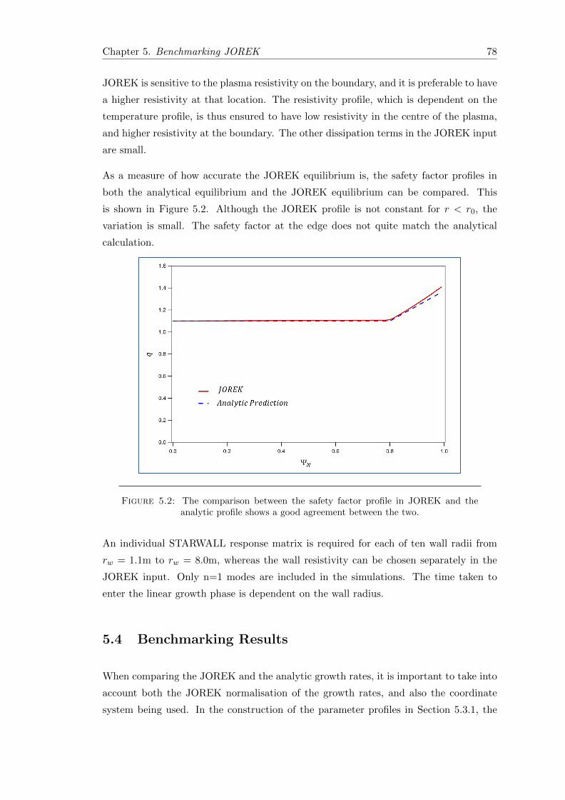
Chapter 5. Benchmarking JOREK 78
JOREK is sensitive to the plasma resistivity on the boundary, and it is preferable to have
a higher resistivity at that location. The resistivity profile, which is dependent on the
temperature profile, is thus ensured to have low resistivity in the centre of the plasma,
and higher resistivity at the boundary. The other dissipation terms in the JOREK input
are small.
As a measure of how accurate the JOREK equilibrium is, the safety factor profiles in
both the analytical equilibrium and the JOREK equilibrium can be compared. This
is shown in Figure 5.2. Although the JOREK profile is not constant for r < r0, the
variation is small. The safety factor at the edge does not quite match the analytical
calculation.
Figure 5.2: The comparison between the safety factor profile in JOREK and theanalytic profile shows a good agreement between the two.
An individual STARWALL response matrix is required for each of ten wall radii from
rw = 1.1m to rw = 8.0m, whereas the wall resistivity can be chosen separately in the
JOREK input. Only n=1 modes are included in the simulations. The time taken to
enter the linear growth phase is dependent on the wall radius.
5.4 Benchmarking Results
When comparing the JOREK and the analytic growth rates, it is important to take into
account both the JOREK normalisation of the growth rates, and also the coordinate
system being used. In the construction of the parameter profiles in Section 5.3.1, the

Chapter 5. Benchmarking JOREK 79
radial coordinate is r. However, in JOREK the parameter profiles are specified with
ψN , the normalised poloidal flux, as the radial coordinate. Thus a step in the current
at r = r0 in the analytic equilibrium needs to be matched to a step at the correct
ψN = ψN,0 in JOREK. In the following results, q0 = 1.1 and the current and density
steps are located at ψN,0 = 0.8.
Ideal Wall Benchmarking
The radius at which an ideal wall will stabilise the ideal kink for the choice of equilibrium
parameters used in the JOREK simulations can be calculated using Equation 5.19. This
radius is found to be ridealw ∼ 1.59. JOREK simulations with an ideal wall at varying
wall radii were performed: the results are shown in Figure 5.3.
Figure 5.3: Comparison of JOREK and analytic predictions for ideal kink growthrates. The marginal wall radius at which the ideal kink is stabilised is found in JOREK.
The marginal wall radius ridealw in JOREK is found to agree with Equation 5.19. The
JOREK simulations calculate a slightly lower growth rate than the analytic prediction
(especially at large wall radius), but exhibit the correct behaviour. This implies that
JOREK does not agree with the analytic results in the absence of the wall, but does
not imply that the implementation of the resistive wall in JOREK is incorrect. The
difference between analytic and JOREK growth rate is not constant, so normalisation
is not the issue here.

Chapter 5. Benchmarking JOREK 80
5.4.1 Resistive Wall Benchmarking
The ideal wall was replaced with a resistive wall, with resistivities ranging from 2.5 ×10⁻¹Ωm to 2.5× 10⁻⁶Ωm. Figure 5.4 shows the JOREK growth rates for the full range
of wall radii. The growth rates show the expected behaviour for a RWM as the resistive
wall is moved further from the plasma: the stabilising influence of the wall is reduced
and the growth rate increases, levelling out as the wall moves to infinity. Additionally,
the more resistive the wall is, the greater the stabilising influence it exerts on the plasma,
as the perturbed magnetic flux is increasingly unable to penetrate the wall.
Figure 5.4: Full benchmarking results over a range of wall resistivities and radii
The JOREK growth rates can be compared to the calculated growth rates, using Equa-
tion 5.17. A comparison between the analytical and JOREK growth rates can be seen
for two different wall resistivities in Figures 5.5 and 5.6. The agreement is reasonably
good: it can be noticed in Figure 5.6, at the lower wall resistivity, a lack of agreement
when the wall is located close to the plasma edge.
This deviation from the analytical growth rate calculation can be attributed to the
resolution of STARWALL. However, doubling the resolution of STARWALL from 16 to
32 poloidal grid points had no effect on the linear growth rate in JOREK, so we cannot
be sure this is the explanation.

Chapter 5. Benchmarking JOREK 81
Figure 5.5: The analytic and JOREK simulation growth rates are, for this wallresistivity, very good.
Figure 5.6: At smaller wall radii, JOREK finds larger growth rates than the analyticestimate, but only when the resistivity is low.

Chapter 5. Benchmarking JOREK 82
Figure 5.7: The inclusion of the inertia correction into the analytic growth rateequation is crucial for calculating the growth rate for larger wall radii.
Inclusion Of Plasma Inertia
When the resistive wall is located at rw > ridealw , the inertia contribution is necessary for
predicting the correct growth rate. The right hand side of Equation 5.17 describes the
inertia contribution to the mode growth rate. Neglecting the right hand side of Equation
5.17 will allow the growth rate of the RWM to be found when the inertia contribution
is negligible.
The inertia is important for larger wall radii, where rw > ridealw . The stability of the
resistive wall mode is determined by the wall eddy currents, not the plasma inertia;
the inertia term can be neglected for close-fitting walls. However, the plasma inertia
is important for ideal kink stability. The ideal kink is unstable when rw > ridealw , as
described above in Section 5.3.1.
Without the inertia contribution, the dispersion relation is linear, and thus straightfor-
ward to solve for the growth rate of the mode. With the inclusion of the inertia term,
the equation is cubic in γ. One solution will correspond to the RWM, and the two com-
plex conjugate solutions correspond to the plasma mode. The three roots of the cubic
Equation 5.17 can be found numerically. The initial guess for a solution is provided by
solving Equation 5.17 with the inertia contribution set to zero. Then, an iteration with
this value of γ as an initial guess is used to find the first root of the equation. Once the
first root is known, Equation 5.17 can be reduced to a quadratic and solved directly for
the remaining roots.
Figure 5.7 shows the results of including the inertia term for a range of wall radii. For
wall radii such that rw < ridealw , inertia is not a significant contribution to the calculation
of the growth rate of the mode. As shown by the dark blue markers, the JOREK growth

Chapter 5. Benchmarking JOREK 83
rate and the analytic calculation excluding the inertia term agree well. For larger wall
radii, the dark blue markers showing the analytic growth rate without inertia included
disagree substantially with the JOREK results. The inclusion of inertia resolves the
discrepancy.
5.5 Summary Of Results
In this chapter, the implementation of the resistive wall in JOREK was discussed. The
inclusion of the resistive wall is achieved by coupling JOREK to STARWALL. By using
a linear model for a RWM, the growth rates found in JOREK simulations could be
compared against calculated rates. This benchmark was successful. JOREK agreed
with the linear model as to the wall radius at which an ideal wall would stabilise the
ideal kink. There was also good agreement when the wall was resistive: though when the
wall resistivity is low, some disagreement was found which is as yet fully unaccounted
for. This benchmark supports the work described in [115].

Chapter 6
ITER simulations with JOREK
and realistic wall
6.1 ITER Equilibrium
The inclusion of the resistive wall is useful while investigating the non-linear MHD
physics in ITER advanced scenarios. The key features that need to be included in the
equilibrium are the reversed safety factor profile and a sufficiently high βN (above the no-
wall limit). The plasma current should be around 9MA, and βN projected to be ∼ 2.9.
Previous simulations of the advanced scenarios for ITER can be found in [119, 120].
The walls are modelled as thin shells. The first is an approximation to the ITER first
wall, whilst the second is closer-fitting than the ITER first wall. The two walls used are
shown in Figure 6.1. A no wall situation can be simulated by setting the wall resistivity
very high (∼ 109) - the JOREK default without STARWALL coupling is an ideal wall at
the plasma separatrix. The following simulations are carried out with the only toroidal
mode number as n=1. The STARWALL matrix is generated for a particular set of mode
numbers; changing the mode numbers requires a new STARWALL matrix.
6.1.1 Reducing The Edge Current
The initial equilibrium was set up with a reversed shear safety factor profile, with a
minimum safety factor value of 1.5, a current of ∼ 9 MA and βN = 2.2. When the time
stepping was implemented with the ITER-like wall, the eigenfunction of the unstable
mode, shown in Figure 6.2, is highly localised at the edge of the plasma. In contrast, the
RWM is a global mode and the displacement is expected to be across the whole plasma.
84

Chapter 6. JOREK Simulations 85
Figure 6.1: Location of the ITER-like wall in STARWALL (courtesy of M. Holzl).
When the wall is moved closer to the plasma (the second wall in Figure 6.1), the edge
mode has the same amplitude- the localisation of the displacement does not extend far
enough outside the plasma to be affected by the resistive wall. It is difficult to move the
wall even closer to the plasma, since the wall would interfere with the gridding process
in JOREK.
Since the location of the wall does not affect the unstable edge mode, the stability and
structure of the mode can be affected by altering its drive. The drive for the edge mode
is the edge current. The current profile across the plasma is shown in Figure 6.4a). The
current density is prescribed by two variables: the radial pressure gradient p′(ψ) and the
FF′(ψ) profile, where F (ψ) = RBφ. The FF′ profile is a direct JOREK input, however
the radial pressure gradient cannot be manually set, and must be manipulated via the
temperature and density input profiles. Altering the FF′ profile is ineffective in reducing
the edge current- the FF′ profile is shown in Figure 6.3 in blue. This is because here βθ
is close to unity.
The temperature pedestal at the edge is changed instead. This will then change the p′
at the edge, and thus the current density at that location. If the pedestal is sharpened,

Chapter 6. JOREK Simulations 86
Figure 6.2: The n = 1 flux displacement for the first simulations, with βN = 2.2.This unstable mode is located at the edge of the plasma. The RWM is, however, a
global mode.
Figure 6.3: FF′ and p′ profiles for the first simulations. Changing the p′ profile atedge is necessary to alter the mode structure at that location.
then the p′ profile is deeper and the edge current is reduced. The remainder of the
profile is unchanged. Figure 6.4A shows the difference between the two current profiles.
It can be noted in Figure 6.4B that the current profile is hollow. This is necessary to
form the reversed shear safety factor profile, and is a key feature of advanced tokamak
scenarios.
With the edge current reduced, the previous edge mode is stabilised and a global mode
can be found. However, the βN in this simulation is low, at βN = 2.2. The βN can be
raised by scaling the magnetic field. This also results in translating the safety factor
profile, as shown in Figure 6.5. It is crucial to keep the minimum safety factor greater
than 1, to avoid MHD instabilities at the q = 1 rational surface. Scaling the toroidal

Chapter 6. JOREK Simulations 87
Figure 6.4: Figures showing the current profiles in the simulations. a) The reductionin edge current is shown in this figure. This is sufficient to stabilise the edge modemanifesting in the simulations; and b)the poloidal cross section shows the hollow current
profile necessary for a reversed shear q profile.

Chapter 6. JOREK Simulations 88
magnetic field through the parameter F0 = RBφ changes βN to βN = 2.6. This is still
not as high as many advanced scenarios, but substantially closer to them.
Figure 6.5: Scaling the magnetic field increases βN to 2.6, but also translates thesafety factor profile. The poloidal β remains constant when the q profile is changed -
it is the toroidal β which is increased.
6.2 Features Of The Unstable Mode
After establishing an equilibrium with suitable parameters, the equilibrium can be
evolved in time. However, after a certain number of time steps, a numerical instability
prevents further evolution. Instead of entering a linear growth phase after an initial
period of energy oscillation, the energy contained by the n=1 perturbation is subject to
a numerical instability, which grows until it dominates the evolution. A discontinuity is
seen in the time evolution of the n=1 energy and no further time steps are possible -
JOREK is unable to converge on the next time step. This numerical instability is shown
in Figure 6.6, where the n = 1 component of the kinetic energy has been plotted.
JOREK calculates the magnetic and kinetic energies as a function of time, for each
Fourier harmonic. The energy can be used as an indication of the instability of the
mode: an exponential growth in the energy corresponds to a constant growth of the
mode. This growth rate can be calculated from the slope of the logarithm of the energy.
At time steps t1, t2 with energies E1, E2 respectively, the growth rate (in JOREK units)
is found by γJOREK = (ln(E2)− ln(E1))/(t2 − t1).
The energy is calculated as two components: magnetic and kinetic energies. These
are calculated respectively from the poloidal magnetic field Bθ, and the product of the
density ρ with the poloidal velocity vθ. Bθ is calculated from the poloidal magnetic
flux function, and vθ from the stream function u. The kinetic energy is the energy used
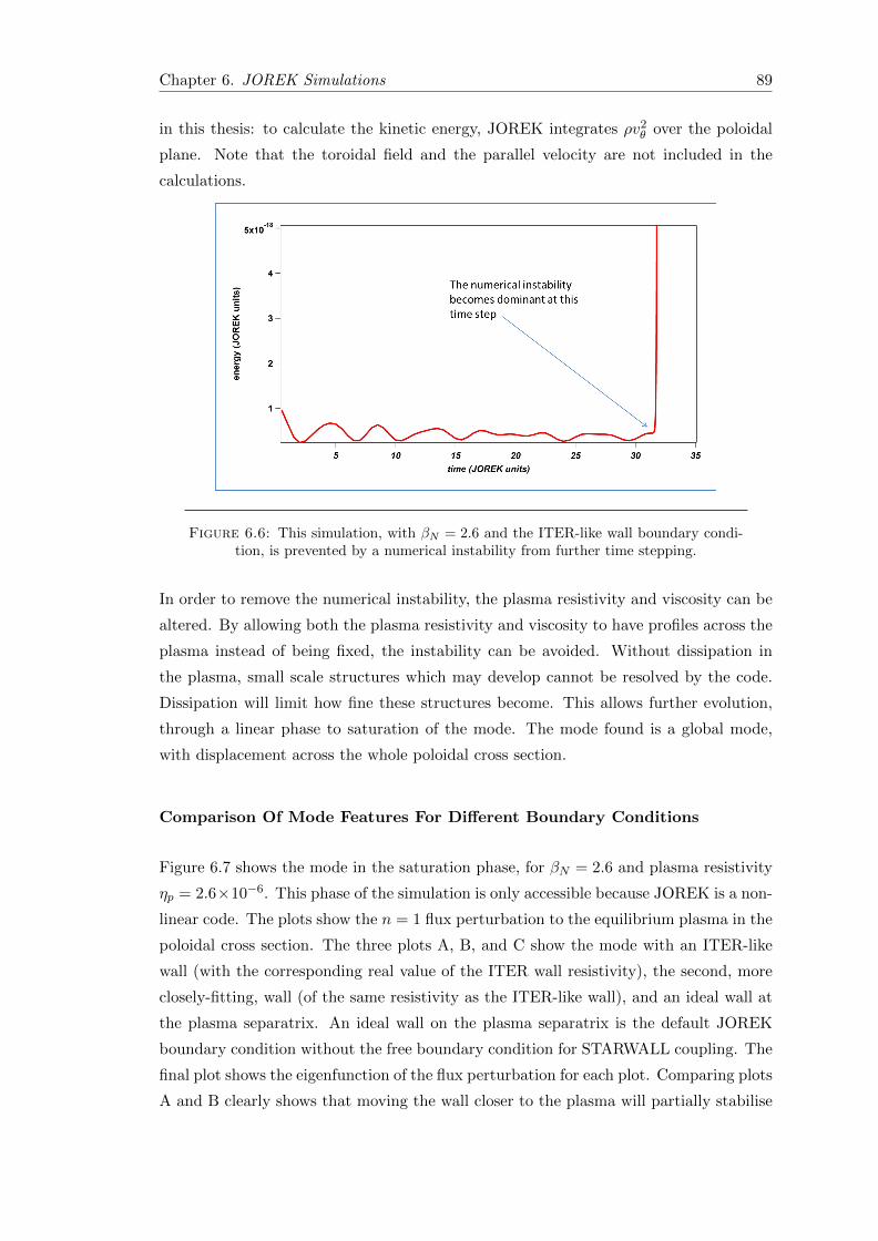
Chapter 6. JOREK Simulations 89
in this thesis: to calculate the kinetic energy, JOREK integrates ρv2θ over the poloidal
plane. Note that the toroidal field and the parallel velocity are not included in the
calculations.
Figure 6.6: This simulation, with βN = 2.6 and the ITER-like wall boundary condi-tion, is prevented by a numerical instability from further time stepping.
In order to remove the numerical instability, the plasma resistivity and viscosity can be
altered. By allowing both the plasma resistivity and viscosity to have profiles across the
plasma instead of being fixed, the instability can be avoided. Without dissipation in
the plasma, small scale structures which may develop cannot be resolved by the code.
Dissipation will limit how fine these structures become. This allows further evolution,
through a linear phase to saturation of the mode. The mode found is a global mode,
with displacement across the whole poloidal cross section.
Comparison Of Mode Features For Different Boundary Conditions
Figure 6.7 shows the mode in the saturation phase, for βN = 2.6 and plasma resistivity
ηp = 2.6×10⁻⁶. This phase of the simulation is only accessible because JOREK is a non-
linear code. The plots show the n = 1 flux perturbation to the equilibrium plasma in the
poloidal cross section. The three plots A, B, and C show the mode with an ITER-like
wall (with the corresponding real value of the ITER wall resistivity), the second, more
closely-fitting, wall (of the same resistivity as the ITER-like wall), and an ideal wall at
the plasma separatrix. An ideal wall on the plasma separatrix is the default JOREK
boundary condition without the free boundary condition for STARWALL coupling. The
final plot shows the eigenfunction of the flux perturbation for each plot. Comparing plots
A and B clearly shows that moving the wall closer to the plasma will partially stabilise

Chapter 6. JOREK Simulations 90
the mode: the eigenfunction amplitude is smaller and the poloidal cross sections show
that although the displacement has a similar structure, it has been reduced by the closer-
fitting wall. Comparison with the mode when an ideal wall is placed at the ITER wall
location in plot C of Figure 6.7 shows that the ideal wall stabilises the global mode,
with perturbations localised at the vertical extremes of the plasma. These structures
at the top and bottom of the plasma shown in Figure 6.7 for the ideal wall on the
separatrix are also seen in the linear phase of growth for the simulation. The flux
perturbation is again much smaller with this wall, as shown in the eigenfunction plot D.
These plots show that firstly, the mode is external as the wall boundary condition affects
its evolution; and secondly, that it is a global mode. This provides evidence that the
mode we are simulating is indeed a RWM. In addition, in Figure 6.7, Plot D contains
the n = 1 eigenfunction extracted from the poloidal flux perturbation plots A-C. The
flux eigenfunction is taken at the location of the horizontal lines in the poloidal plots -
the same location for each case. Plot D shows the relative magnitude and extent of the
eigenfunctions - the perturbation is shown to extend over the poloidal plane for Plots
A and B.), and the magnitude of the eigenfunction is smaller for the closer wall. The
growth rate of the mode for different wall resistivities is discussed below in Section 6.2.2.
6.2.1 Plasma Resistivity Scan
The plasma resistivity is an important parameter to bear in mind whilst performing
these large-scale MHD simulations, as can be seen in Section sec:featuresunstable where
altering the plasma resistivity can resolve the numerical difficulties associated with in-
appropriate dissipation levels in the simulation. Although the RWM is not a resistive
instability and its growth rate should not depend on the plasma resistivity, the use of
plasma resistivity should be investigated in order to find how the simulation will be
affected by it.
In order to investigate the mode stability, the plasma resistivity can be scanned while
keeping βN = 2.6 and using the ITER-like wall as the boundary condition. Previous
simulations were carried out at a plasma resistivity ηp = 2 × 10⁻⁶ (this is given in
JOREK-normalised units, which are given by ηSI = ηJOREK√µ0/ρ0 where ρ0 is the
central density of the plasma). This results in a range of growth rates. The point
where the plasma becomes stable can be seen in Figure 6.8. For plasma resistivities less
than ∼ ηp = 1.4 × 10⁻⁷, the plasma is stable, and the energy only oscillates instead of
entering the linear growth phase. For plasma resistivities greater than this value, the
plasma is unstable and the mode is able to grow. Figure 6.9 shows the growth rates
for the simulations which vary plasma resistivity. It can be seen that for small plasma

Chapter 6. JOREK Simulations 91
Figure 6.7: Comparison of saturated modes for βN = 2.6 and different wall configura-tions A, B, and C: ITER-like wall, closely-fitting wall and ideal wall on the separatrix,respectively. Plots A and B have the same wall resistivity.The poloidal plots show then = 1 flux perturbation. Moving the wall closer to the plasma partially stabilises themode, whilst the ideal wall seems to stabilise global perturbations. Plot D shows then = 1 flux eigenfunction plotted across the poloidal cross section (indicated by the
horizontal lines in Plots A, B and C).

Chapter 6. JOREK Simulations 92
resistivities, the growth rate is negative: increasing the plasma resistivity increases the
growth rate. For sufficiently large plasma resistivity, the growth rate becomes positive.
Figure 6.8: Energies for n = 1 (kinetic) for different plasma resistivities, with theITER-like wall as a boundary condition and βN = 2.6. Reducing the plasma resistivityreduces the mode drive and the results in a slower growth rate. The marginal stabilitypoint in plasma resistivity is an order of magnitude smaller than the value used in
preceding simulations.
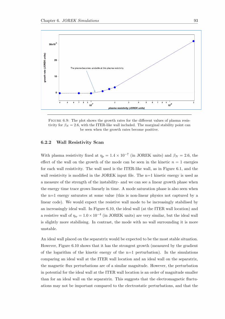
Chapter 6. JOREK Simulations 93
Figure 6.9: The plot shows the growth rates for the different values of plasma resis-tivity for βN = 2.6, with the ITER-like wall included. The marginal stability point can
be seen when the growth rates become positive.
6.2.2 Wall Resistivity Scan
With plasma resistivity fixed at ηp = 1.4 × 10⁻⁷ (in JOREK units) and βN = 2.6, the
effect of the wall on the growth of the mode can be seen in the kinetic n = 1 energies
for each wall resistivity. The wall used is the ITER-like wall, as in Figure 6.1, and the
wall resistivity is modified in the JOREK input file. The n=1 kinetic energy is used as
a measure of the strength of the instability- and we can see a linear growth phase when
the energy time trace grows linearly in time. A mode saturation phase is also seen when
the n=1 energy saturates at some value (this is non-linear physics not captured by a
linear code). We would expect the resistive wall mode to be increasingly stabilised by
an increasingly ideal wall. In Figure 6.10, the ideal wall (at the ITER wall location) and
a resistive wall of ηw = 1.0× 10⁻⁴ (in JOREK units) are very similar, but the ideal wall
is slightly more stabilising. In contrast, the mode with no wall surrounding it is more
unstable.
An ideal wall placed on the separatrix would be expected to be the most stable situation.
However, Figure 6.10 shows that it has the strongest growth (measured by the gradient
of the logarithm of the kinetic energy of the n=1 perturbation). In the simulations
comparing an ideal wall at the ITER wall location and an ideal wall on the separatrix,
the magnetic flux perturbations are of a similar magnitude. However, the perturbation
in potential for the ideal wall at the ITER wall location is an order of magnitude smaller
than for an ideal wall on the separatrix. This suggests that the electromagnetic fluctu-
ations may not be important compared to the electrostatic perturbations, and that the
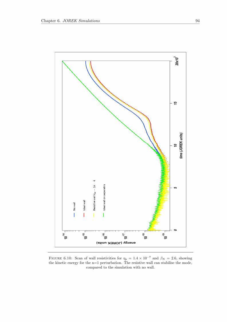
Chapter 6. JOREK Simulations 94
Figure 6.10: Scan of wall resistivities for ηp = 1.4 × 10⁻⁷ and βN = 2.6, showingthe kinetic energy for the n=1 perturbation. The resistive wall can stabilise the mode,
compared to the simulation with no wall.

Chapter 6. JOREK Simulations 95
mode found when the ideal wall is placed on the separatrix is not essentially an MHD
mode.
6.2.3 βN Scan
The mode stability can be also be explored by changing βN , and keeping the ITER-like
wall as the boundary condition. Increasing βN would be expected to increase the mode
growth rate, since it corresponds to increasing the pressure. As βN is not a direct JOREK
input parameter, but calculated by JOREK after solving the plasma equilibrium, βN
must be indirectly manipulated by varying the toroidal magnetic field in the plasma.
This changes the safety factor profile, which also affects the mode drive. The parameter
F0 = RBφ in the JOREK input file is used to scale the toroidal magnetic field.
The first attempt to scan βN was made only by scaling the magnetic field. This creates
a family of safety factor profiles, with identical shapes but with the minimum safety
factor value at different distances from q = 1. This alters the drive of the mode for
each value of βN found, which means the growth rates for each case were incomparable.
Instead, it proved to be more useful to scale the magnetic field by changing F0, and then
to scale the magnitude of the plasma pressure profile. Changing these two parameters
can together scale βN , and retain a constant minimum safety factor profile. Although
the safety factor profiles are not identical for each separate βN case, they are similar,
and vary over a small enough range, that the growth rates can be compared over a small
range of βN .
Figure 6.11 shows the JOREK growth rate for a range of βN with the same boundary
condition of the ITER-like wall. As expected, an increase in βN corresponds to an
increase in the growth rate of the mode. Thus, in tokamak operating regimes where
βN is ramped up in order to maximise power generation, the growth rate of the RWM
would be increased also. For βN = 3.5 (not shown in the figure), JOREK obtains a
growth rate of γJ = 4.6, which is 4 orders of magnitude higher than the growth rate for
βN = 2.6.
6.3 Adding Parallel Velocity Profile
JOREK is capable of modelling parallel (to magnetic field lines) velocity by changing
the physics model. The additional equation to be solved is Equation 5.1.2.
A key difference to using the parallel velocity model is the initial simulation of the
equilibrium. In previous simulations, the equilibrium is solved at time t = 0, and
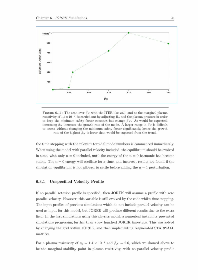
Chapter 6. JOREK Simulations 96
Figure 6.11: The scan over βN with the ITER-like wall, and at the marginal plasmaresistivity of 1.4×10⁻⁷, is carried out by adjusting Bφ and the plasma pressure in orderto keep the minimum safety factor constant but change βN . As would be expected,increasing βN increases the growth rate of the mode. A larger range in βN is difficultto access without changing the minimum safety factor significantly, hence the growth
rate of the highest βN is lower than would be expected from the trend.
the time stepping with the relevant toroidal mode numbers is commenced immediately.
When using the model with parallel velocity included, the equilibrium should be evolved
in time, with only n = 0 included, until the energy of the n = 0 harmonic has become
stable. The n = 0 energy will oscillate for a time, and incorrect results are found if the
simulation equilibrium is not allowed to settle before adding the n = 1 perturbation.
6.3.1 Unspecified Velocity Profile
If no parallel rotation profile is specified, then JOREK will assume a profile with zero
parallel velocity. However, this variable is still evolved by the code whilst time stepping.
The input profiles of previous simulations which do not include parallel velocity can be
used as input for this model, but JOREK will produce different results due to the extra
field. In the first simulations using this physics model, a numerical instability prevented
simulations progressing further than a few hundred JOREK timesteps. This was solved
by changing the grid within JOREK, and then implementing regenerated STARWALL
matrices.
For a plasma resistivity of ηp = 1.4 × 10⁻⁷ and βN = 2.6, which we showed above to
be the marginal stability point in plasma resistivity, with no parallel velocity profile

Chapter 6. JOREK Simulations 97
specified, JOREK now finds an instability that initially grows but then shrinks away.
This suggests that in this model where the parallel flow is evolved, the plasma resistivity
is not sufficiently large enough to observe the mode grow and saturate. The parallel
velocity perturbation plot is shown in Figure 6.12.
Increasing the plasma resistivity should increase the drive of the instability. If the plasma
resistivity is increased to ηp = 2.0×10⁻⁷, then the instability is again found. as shown in
Figure 6.13. After the initial simulation period, when only the n = 0 equilibrium com-
ponent is included to allow the equilibrium with parallel flow to establish, the instability
begins to grow. Instead of dying away as in Figure 6.12, the instability has sufficient
drive to begin to grow exponentially. Unfortunately, a numerical instability at the end
of the simulation prevents the simulation proceeding sufficiently far for the saturation
of the mode to be found. When a rotation profile is added, the numerical instability
ends the simulation in even fewer timesteps. Further work is required to remove this
numerical problem, and complete a simulation through to saturation of the mode.
6.4 Summary Of Results
JOREK is used to simulate advanced tokamak plasmas in an ITER geometry. Coupled
to STARWALL, the wall is modelled as the ITER first wall with the corresponding
resistivity. A plasma equilibrium is constructed which is unstable to the Resistive Wall
Mode. The effects of changing both the plasma resistivity and the wall resistivity are
shown. The βN of the plasma can also be varied by scanning the toroidal magnetic
field. Initial simulations with a physics model which includes parallel (to the magnetic
field line) velocity are carried out, which show that the different physics model affects
the mode stability boundaries. A slightly higher plasma resistivity is required to find
an unstable mode, but numerical problems during the linear growth phase prevent the
simulations entering the saturation phase.

Chapter 6. JOREK Simulations 98
Figure 6.12: Plot A shows the parallel velocity perturbation for a JOREK simulationwith ηp = 1.4 × 10⁻⁷ and no initial velocity profile chosen. For the previous physicsmodel, this value of plasma resistivity was at marginal stability. With parallel velocityincluded, the mode is not unstable and so does not enter a linear growth phase. Theenergy plot in B shows that the n = 1 mode does not enter a linear growth phase, and
in fact shrinks away.

Chapter 6. JOREK Simulations 99
Figure 6.13: The figure shows both the n = 0 and n = 1 kinetic energy componentsof the simulation, which has ηp = 2.0 × 10⁻⁷ and βN = 2.6. The simulation is runwith n = 0 only until the equilibrium becomes stable, then the n = 1 perturbationis included. The instability grows, and begins to enter the linear phase at t ∼ 1900.However, the numerical instability, seen most clearly in the n = 0 component, prevents
the simulation progressing.

Chapter 7
Conclusions And Outlook
Conclusions
In order for nuclear fusion to become a viable power generation method, the development
of cost-competitive and reliable reactors is necessary. A step towards this goal is the
conception of advanced tokamak scenarios. These operating scenarios aim to optimise
the non-inductive current, and achieve steady state tokamak operation.
However, the optimised profiles (such as current and density profiles) in advanced sce-
narios position the operating scenarios close to MHD stability boundaries; and it is
expected that without mitigation, MHD modes may become unstable. This would re-
sult in plasma degradation, and possibly costly disruptions. In addition, the use of
negative ion sources in the neutral beams (which is required to meet energy needs) will
result in high energy beams, with less momemtum in the beam for a given power than
current beams. This development in operating conditions from present to future toka-
maks presents a challenge to the fusion community. Thus, a better understanding of
the stability of modes whose stability is affected by the level of plasma rotation, such
as the Resistive Wall Mode, will be needed in order to understand the results of future
experiments, and to try to mitigate or stabilise the modes.
Non-linear effects are very important for studying MHD modes. The inclusion of non-
linearity is necessary for modelling mode saturation, as well as the coupling of MHD
modes. Non-linear modelling is also needed to understand the interaction of plasma
rotation with the growth of MHD modes. In this thesis, non-linear modelling is carried
out both analytically and with simulations.
In Chapters 3 and 4, the analytic model coupled two MHD instabilities: the Neoclassical
Tearing Mode and the Resistive Wall Mode. A set of coupled non-linear equations was
100

Chapter 7. Conclusions And Outlook 101
derived by considering three regions in the system: the ideal plasma regions, the resistive
wall, and the rational layer where the magnetic island is located. These equations were
solved, firstly by finding a limiting analytic solution for small islands, and secondly
numerically. The equations could also be integrated numerically in order to obtain
mode growth rates, frequencies, and plasma rotation frequencies as a function of time.
Chapters 5 and 6 describe non-linear simulations using JOREK. The inclusion of the
code STARWALL into JOREK allows for simulations of plasmas with resistive wall
boundary conditions. Chapter 5 describes the benchmarking carried out against a linear
RWM dispersion relation, which successfully shows the agreement between JOREK and
the linear model. Chapter 6 shows JOREK simulations in an ITER geometry using a
resistive wall which is based on the ITER first wall. An equilibrium is found which is
unstable to the RWM, and initial simulations are carried out showing the features of the
mode with respect to plasma resistivity, wall resistivity and βN . Attempts to include a
more complex physics model in JOREK, which incorporates plasma flow parallel to the
magnetic field lines, are also briefly included. These simulations for a plasma with flow
show that the plasma marginal stability is located at slightly different parameters when
the physics model is changed.
Future Work
Substantial scope for future work can be found in the work presented in this thesis, both
in the analytic modelling and JOREK simulations.
In the analytic modelling, it is possible to extend the model to include error field effects
on the NTM. Error fields are small variations in the magnetic field which are unintended,
but result from misaligned field coils. The misalignment could be caused by manufac-
turing or engineering issues. Error fields can be resonant with modes in the plasma,
and are known to exacerbate mode instability. They are also responsible for exerting
a drag on the plasma, slowing the plasma rotation. There are a number of theoretical
works which study the link between RWMs and error fields: including that of Gimblett
and Hastie detailed in Appendix B. In [35], it can be seen that the equivalent to ∆W
at the wall for the error field coil is ∆coil = −imI/ψE where ψE is the helical flux at
the coil location (and is a function of the plasma equilibrium), and I is the measure of
the helical current responsible for the error field. The system would be solved for the
amplitude and phase of ψE . Additionally, the relationship between the layer ∆L and
the error field coil ∆E is identical to that between ∆L and ∆W . The implemetation of
the coupling between rational layer and error field coil would be thus similar to that
of the coupling between rational layer and resistive wall. It could be expected that the
Chapter 7. Conclusions And Outlook 102
magnitude of the error field affects the NTM island threshold width, and it may provide
another explanation for the observation of triggerless NTMs.
The implementation of the JOREK-STARWALL coupling, and the ability to model 3D
resistive walls in a realistic geometry, is a foundation for simulating not only RWMs but
also other modes such as ELMs, and Vertical Displacement Events (discussed in [115]).
In terms of modelling Resistive Wall Modes, the addition of the wall is important for
understanding the interaction of resistive wall and rotating plasma. In particular, the
simulations with ideal walls on the separatrix, which produced growth rates much higher
than expected, should be investigated to understand the reasons why the simulations
are not as would be expected.
Using JOREK with a physics model that includes parallel (i.e. along magnetic field
lines) flow allows for exploring this interaction. Simulations of advanced tokamak plas-
mas (specifically for ITER scenarios) with plasma flow included, can assist with un-
derstanding the effects of the low rotation rate in these scenarios. Once the numerical
instability is removed from the simulations, further work would include modelling the
effects of varying the parallel rotation profile on the growth of the RWM; and conversely,
the effect of the growth of the RWM on the parallel rotation profile.
Furthermore, it could be possible to investigate the analytic model explored in Chapter
3 and Chapter 4. This could be achieved by seeding a magnetic island at a rational
surface using the FF′
input profile. A spike in this profile would result in an island
forming in the plasma, which would remain unstable to the RWM also. The effect of
plasma rotation could then be examined in JOREK with the resistive wall included.

Appendix A
RWM Dispersion Relation Using
Variational Principle
The following derivation is given in Haney and Freidberg [30]. Using the Energy Princi-
ple, Haney and Freidberg [30] derived a dispersion relation for the RWM, requiring only
knowledge of the behaviour of the system with the ideal wall.
The stability of a plasma is calculated by using the Energy Principle. A plasma is stable
if, for all plasma displacements ξ, the plasma energy ∂W > 0. The plasma is unstable
if there exists a physically allowed displacement such that ∂W < 0.
Ideal Wall At Infinity
Suppose an ideal wall is located at infinity: then the plasma energy can be expressed as
∂W∞ = ∂WF + ∂W∞V (A.1)
where ∂WF is the fluid energy integrated over the volume of the plasma, and ∂W∞V is
the vacuum energy integrated over the vacuum region surrounding the plasma.
∂WF = 12
∫Vp
(|∂B|2µ0− ξ · (J× ∂B) + γp|∇ · ξ|2 + (ξ · ∇p)∇ · ξ
)dV (A.2)
∂W∞V = 12
∫V∂B∞µ0
dV (A.3)
It has been assumed that no surface currents flow in the plasma boundary so there is
no contribution from the surface energy. ∂WF can be found easily given a trial function
ξ. To deal with ∂WV , the vacuum magnetic field is expressed as a vector potential:
103

Appendix A. RWM Dispersion Relation 104
∇× ∂A∞, with ∂A∞ satisfying ∇×∇× ∂A∞ = 0. The boundary conditions used are
∂A∞|∞ = 0 and, if en is the outward facing unit normal to the surface of the plasma,
Sp, en × ∂A∞|Sp = −(en · ξ)B|Sp . This is the linearised jump condition for the electric
field across the plasma surface. (The pressure jump condition is considered to be ‘as
good as’ satisfied as part of the variational method.)
Equation A.3 can be rewritten as
∂W∞V =1
2µ0
∫Sp
(en × ∂A∞) · en × (en ×∇× ∂A∞)dS (A.4)
Assume that the system is unstable with the wall at infinity: that it, ∂W∞ < 0.
Ideal Wall At Finite Radius
Now consider a closed, ideal wall of arbitrary shape, a finite distance from the plasma,
where the surface of the wall is Sb. The plasma displacement ξ (i.e. the trial function
in the variational method) is identical to the displacement with a wall at infinity.
The potential energy can now be written ∂Wb = ∂WF +∂W bV , where ∂WF has the same
value as when the wall is at infinity. Assume that the potential energy ∂Wb > 0, such
that the system is stabilised by the ideal wall at a finite distance from the plasma. In
addition,
∂W bV =
1
2µ0
∫Sp
(en × ∂Ab) · en × (en ×∇× ∂Ab)dS (A.5)
such that ∇×∇× ∂Ab = 0 with the analogous boundary conditions en × ∂A∞|Sb = 0,
and en × ∂A∞|Sp = −(en · ξ)B|Sp . The boundary conditions are slightly different due
to the presence of the ideal wall at finite radius.
Assume that the system is stable with the ideal wall at this finite radius: that is,
∂Wb > 0.
Resistive Wall At Finite Radius
The ideal wall at Sb is replaced by a resistive wall of conductivity σ and thickness d,whilst
keeping the same trial function ξ. Now ∂Wb = ∂WF + ∂W bV , where ∂WF has the same
value as above. The analysis hinges on the assumptions: firstly that the growth rate of
the RWM is comparable to the characteristic wall diffusion time τw = µ0σdb, where b is
the average radius of the vacuum chamber. Thus
γ << γMHD (A.6)

Appendix A. RWM Dispersion Relation 105
where γMHD = −∂W∞/K is the characteristic ideal MHD growth rate with the wall at
infinity. Additionally, the wall is assumed to be ‘thin’: d << b. These assumptions imply
that plasma inertia effects are negligible on relevant timescales. Thus the linearised ideal
MHD force operator as a function of the plasma displacement is F(ξ) = 0. This can be
used to write a Lagrangian for the plasma surrounded by a resistive wall:
L =
∫Vp
ξ · F(ξ)dV = 0 (A.7)
or
L = ∂WF +1
2
∫Sp
(en · ξ)(
B · ∂B
µ0
)dS (A.8)
By calculating jump conditions over the resistive wall, L can be written
∂WF + ∂W iV + ∂W o
V +σγd
2
∫Sb
|en × ∂A|2dS (A.9)
where A refers to vacuum quantities, and the subscripts i, o refer to the inner (between
wall and plasma) and outer (beyond wall) vacuum regions. In the limit of marginal
stability, γ → 0, the Lagrangian reduces the ideal MHD potential energy, with a wall at
infinity ∂W∞.
Using properties of the vacuum solutions, and the variational variable c, L is expressed
as [30]
L = ∂W∞ + c2(∂Wb − ∂W∞) +σγd(1− c)2
2
∫Sp
|en × A∞|2dS (A.10)
This is quadratic in c, which can be eliminated by solving ∂L/∂c = 0. Setting L = 0,
the dispersion relation
γτw = −∂W∞∂Wb
(A.11)
can be found, where τw = µ0σbd, such that b is the average radius of the vacuum
chamber.

Appendix A. RWM Dispersion Relation 106
Equation A.11 shows that, for a system unstable with the wall at infinity, but stable
with an ideal wall sufficiently close to the plasma, is always unstable to a slowly growing
mode (RWM) if the ideal wall is replaced by a resistive wall.

Appendix B
Gimblett And Hastie RWM
Model
The analytical model in [35, 55] is similar to that used in Chapters 3, 4. The technique of
linking resistive, rational layers together through ideal MHD regions is used extensively
in the literature (as in [121], for example).
In this case, the use of the rational layer, and the growth of a magnetic island there, is
necessary to allow the inclusion of the torque balance relation. Analogously to the model
developed in this thesis, the wall response is modelled as the thin wall approximation
[100]. However, in the Gimblett and Hastie model, the layer response differs that used
in this thesis. In this thesis, the growth of the magnetic island is determined by the
non-linear NTM physics, in [55] the layer response is visco-resistive [122].
∆′
= (pτL)54 (B.1)
where τL is the characteristic resistive layer time [77]. This response can be compared
to the layer response obtained in Chapter 3
4w = Re[∆L] + βw
(1− w2
cw2
)(B.2)
2w(ω − ΩL) + Im[∆L] = 0 (B.3)
which describes the NTM evolution.
107
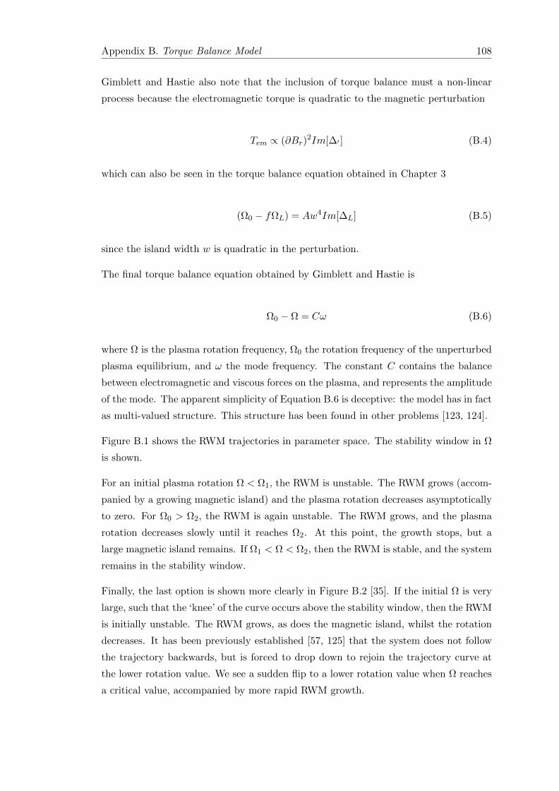
Appendix B. Torque Balance Model 108
Gimblett and Hastie also note that the inclusion of torque balance must a non-linear
process because the electromagnetic torque is quadratic to the magnetic perturbation
Tem ∝ (∂Br)2Im[∆′ ] (B.4)
which can also be seen in the torque balance equation obtained in Chapter 3
(Ω0 − fΩL) = Aw4Im[∆L] (B.5)
since the island width w is quadratic in the perturbation.
The final torque balance equation obtained by Gimblett and Hastie is
Ω0 − Ω = Cω (B.6)
where Ω is the plasma rotation frequency, Ω0 the rotation frequency of the unperturbed
plasma equilibrium, and ω the mode frequency. The constant C contains the balance
between electromagnetic and viscous forces on the plasma, and represents the amplitude
of the mode. The apparent simplicity of Equation B.6 is deceptive: the model has in fact
as multi-valued structure. This structure has been found in other problems [123, 124].
Figure B.1 shows the RWM trajectories in parameter space. The stability window in Ω
is shown.
For an initial plasma rotation Ω < Ω1, the RWM is unstable. The RWM grows (accom-
panied by a growing magnetic island) and the plasma rotation decreases asymptotically
to zero. For Ω0 > Ω2, the RWM is again unstable. The RWM grows, and the plasma
rotation decreases slowly until it reaches Ω2. At this point, the growth stops, but a
large magnetic island remains. If Ω1 < Ω < Ω2, then the RWM is stable, and the system
remains in the stability window.
Finally, the last option is shown more clearly in Figure B.2 [35]. If the initial Ω is very
large, such that the ‘knee’ of the curve occurs above the stability window, then the RWM
is initially unstable. The RWM grows, as does the magnetic island, whilst the rotation
decreases. It has been previously established [57, 125] that the system does not follow
the trajectory backwards, but is forced to drop down to rejoin the trajectory curve at
the lower rotation value. We see a sudden flip to a lower rotation value when Ω reaches
a critical value, accompanied by more rapid RWM growth.
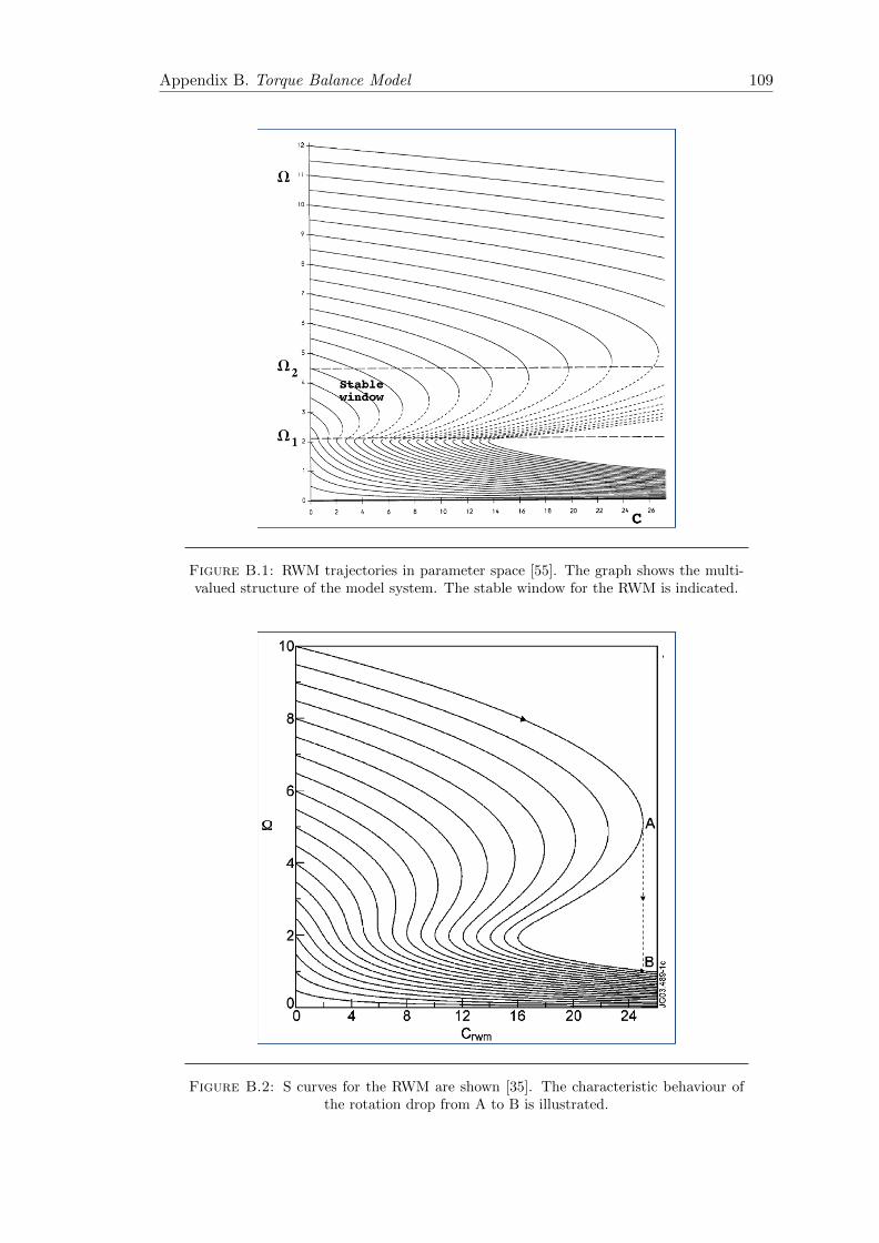
Appendix B. Torque Balance Model 109
Figure B.1: RWM trajectories in parameter space [55]. The graph shows the multi-valued structure of the model system. The stable window for the RWM is indicated.
Figure B.2: S curves for the RWM are shown [35]. The characteristic behaviour ofthe rotation drop from A to B is illustrated.

Appendix B. Torque Balance Model 110
The s-curve behaviour is not seen in the model developed in this thesis. As discussed in
Chapter 4, the resistive wall mode is not sensitive to the plasma rotation - the electro-
magnetic torque is very large at the rational surface.
Bibliography
[1] International Energy Agency. World Energy Outlook. 2013. URL
http://www.worldenergyoutlook.org/pressmedia/recentpresentations/
LondonNovember12.pdf.
[2] International Energy Agency. World Energy Outlook. 2012.
URL http://www.iea.org/newsroomandevents/speeches/
130326FutureEnergyTrendsWEO2012NZrev.pdf.
[3] J. Wesson. Tokamaks. Clarendon Press, 3rd edition. ISBN 978-0198509226.
[4] J. D. Lawson. Some criteria for a power producing thermonuclear reactor. Pro-
ceedings of the Physical Society. Section B, 70(1):6, 1957.
[5] R. J. Bickerton and et al. Nature Phys, Sci,, 229:110, 1971.
[6] C.E. Kessel. Bootstrap current in a tokamak. Nucl. Fusion, 34(9):1221, 1994.
[7] ITER physics basis. Nucl. Fusion, 39:2137, 1999.
[8] Summary of the ITER final design report. ITER EDA Documentation Series No
22 (Vienna: IAEA), 2001.
[9] F Wagner and et al. Regime of improved confinement and high beta in neutral-
beam-heated divertor discharges of the ASDEX tokamak. Phys. Rev. Lett, 49:
1408, 1982.
[10] C. Kessel, J. Manickam, G. Rewoldt, and W. M. Tang. Improved plasma perfor-
mance in tokamaks with negative magnetic shear. Phys. Rev. Lett., 72:1212–1215,
1994.
[11] A C C Sips, for the Steady State Operation, and the Transport Physics topical
groups of the International Tokamak Physics Activity. Advanced scenarios for
ITER operation. Plasma Phys. Contr. Fusion, 47(5A):A19, 2005.
[12] F. M. Levinson. Improved confinement with reversed magnetic shear in TFTR.
Phys. Rev. Lett, 75:4417, 995.
111
Bibliography 112
[13] E. J. Strait and et al. Enhanced confinement and stability in DIII-D discharges
with reversed magnetic shear. Phys. Rev. Lett, 75:4421, 1995.
[14] O. Gruber and et al. Stationary-mode discharges with internal transport barrier
on ASDEX Upgrade. 83:1787, 1999.
[15] T Fujita and the JT-60 Team. High-performance experiments towards steady-state
operation in JT-60U. Plasma Phys. Contr. Fusion, 39:B75, 1997.
[16] J. W. Connor. A review of internal transport barrier physics for steady-state
operation of tokamaks. Nucl. Fusion, 44:R1, 2004.
[17] M. Kikuchi. Steady state tokamak reactor based on the bootstrap current. Nucl.
Fusion, 30(2):265, 1990.
[18] R. C. Wolf and et al. Stationary advanced scenarios with internal transport barrier
on ASDEX Upgrade. Plasma Phys. Contr. Fusion, 41:B93, 1999.
[19] T. C. Luce and et al. Long pulse high performance discharges in the DIII-D
tokamak. Nucl. Fusion, 41:1585, 2001.
[20] A. C. C. Sips. Steady state advanced scenarios at ASDEX Upgrade. Plasma Phys.
COntr. Fusion, 44:B69, 2002.
[21] M. R. Wade and et al. Integrated, advanced tokamak operation on DIII-D. Nucl.
Fusion, 43:634, 2003.
[22] G. T. A. Huysmans and et al. Mhd stability of optimized shear discharges in JET.
Nucl. Fusion, 39:1489, 1999.
[23] Yueqiang Liu, A. Bondeson, Y. Gribov, and A. Polevoi. Stabilization of resistive
wall modes in ITER by active feedback and toroidal rotation. Nucl. Fusion, 44:
232, 2004.
[24] F. Troyon, R. Gruber, H¿ Saurenmann, S. Semenzato, and S. Succi. MHD-limits
to plasma confinement. Plasma Phys. Contr. Fusion, 26:209, 1984.
[25] R. D. Stamburgh and et al. Plasma Phys. Contr. Fusion Research Conf. (London
1984), 1:217, 1984.
[26] E. J. Strait. Stability of high beta tokamak plasmas. Phys. Plasmas, 1:1415, 1994.
[27] D. Pfirsch and H. Tasso. A theorem on MHD-instability of plasmas with resistive
walls. Nucl. Fusion, 11:259, 1971.
[28] A. M. Garofalo and et al. Stabilization of the external kink and control of the
resistive wall mode in tokamaks. Proc. 40th APS Conf. New Orleans, 1998.

Bibliography 113
[29] M. S. Chu and M. Okabayashi. Stabilization of the external kink and the resistive
wall mode. Plasma. Phys. Contr. Fusion, 52:123001, 2010.
[30] S. W. Haney and J. P. Freidberg. Variational methods for studying tokamak
stability in the presence of a thin resistive wall. Phys. Fluids B, 1:1637, 1989.
[31] A. M. Garofalo and et al. Direct observation of the resistive wall mode in a tokamak
and its interaction with plasma rotation. Phys. Rev. Lett., 82:3811, 1999.
[32] H. Reimerdes and et al. Cross-machine comparison of resonant field amplifica-
tion and resistive wall mode stabilization by plasma rotation. Phys. Plasmas, 13:
056107, 2006.
[33] A. C. Sontag and et al. Resistive wall mode stabilization of high-β plasmas in the
National Spherical Torus Experiment. Phys. Plasmas, 12:056112, 2005.
[34] A. M. Garofalo and et al. Resistive wall mode dynamics and active feedback
control in DIII-D. Nucl. Fusion, 41:1171, 2001.
[35] C. G. Gimblett and R. J. Hastie. The interaction of error fields and resistive wall
modes. Phys. Plasmas, 11(3):1019, 2004.
[36] A. Bondeson and D. J. Ward. Stabilization of external modes in tokamaks by
resistive walls and plasma rotation. Phys. Rev. Lett., 72:2709, 1994.
[37] V. D. Shafranov. Sov. Phys. Tech, 15:175, 1970.
[38] R. Betti and J. P. Freidberg. Stability analysis of resistive wall kink modes in
rotating plasmas. Phys. Rev. Lett, 74:2949, 1995.
[39] R. Fitzpatrick and A.Y. Aydemir. Stabilization of the resistive shell mode in
tokamaks. Nucl. Fusion, 36:11, 1996.
[40] J. M. Finn. Stabilization of ideal plasma resistive wall modes in cylindrical geom-
etry: the effect of resistive layers. Phys. Plasmas, 2:3782, 1995.
[41] R. Betti. Beta limits for the n=1 mode in rotating-toroidal-resistive plasmas
surrounded by a resistive wall. Phys. Plasmas, 5:3615, 1998.
[42] A. Bondeson and H. X. Xie. Stability of ideal and resistive modes in cylindrical
plasmas with resistive walls and plasma rotation. Phys. Plasmas, 4:2081, 1997.
[43] B. Coppi, R. Galvao, R. Pellat, M. N. Rosenbluth, and P. H. Rutherford. Sov. J.
Plasma Phys., 2:533, 1976.
[44] J. E. Rice and et al. Toroidal rotation and momentum transport in alcator c-mod
plasmas with no momentum input. Phys. Plasmas, 11:2427, 2004.

Bibliography 114
[45] J. S. deGrassie, J. E. Rice, K. H. Burrell, R. J. Groebner, and W. M. Solomon.
Intrinsic rotation in DIII-D. Phys. Plasmas, 14:056115, 2007.
[46] M. F. F. Nave and J. A. Wesson. Mode locking in tokamaks. Nucl. Fusion, 30:
2575, 1990.
[47] T. C. Hender and et al. Effect of resonant magnetic perturbations on COMPASS-C
tokamak discharges. Nucl. Fusion, 32:2091, 1992.
[48] T. H. Jensen, A. W. Leonard, and A. W. Hyatt. A simple model for driven islands
in tokamaks. Phys Fluids B, 5:1239, 1993.
[49] R. Fitzpatrick. Interaction of tearing modes with external structures in cylindrical
geometry (plasma). Nucl. Fusion, 33:1049, 1993.
[50] R. Fitzpatrick. Bifurcated states of a rotating tokamak plasma in the presence of
a static error-field. Phys. Plasmas, 5:3325, 1998.
[51] R. J. LaHaye and et al. Scaling of the critical plasma rotation for stabilization of
the n = 1 resistive wall mode (ideal kink) in the DIII-D tokamak. Nucl. Fusion,
44, 2004.
[52] E. J. Strait and et al. Wall stabilization of high beta tokamak discharges in DIII-D.
Phys. Rev. Lett., 74:2483, 1995.
[53] E. J. Strait and et al. Resistive wall mode stabilization by slow plasma rotation
in diii-d tokamak discharges with balanced neutral beam injection. Phys Plasmas,
14:056101, 2007.
[54] M. Takechi and et al. Identification of a low plasma-rotation threshold for stabi-
lization of the resistive-wall mode. Phys. Rev. Lett, 98:055002, 2007.
[55] C. G. Gimblett and R. J. Hastie. Theory of Fusion Plasmas. Editrice Compositori,
Bologna, 1999.
[56] R. Fitzpatrick. A simple model of the resistive wall mode in tokamaks. Phys.
Plasmas, 9:3459, 2002.
[57] D. A. Gates and T. C. Hender. Resistive wall induced forbidden bands of mode
rotation frequency on the COMPASS-D tokamak. Nucl. Fusion, 36:273, 1996.
[58] C. M. Bishop. An intelligent shell for the toroidal pinch. Plasma Phys. Contr.
Fusion, 31:1179, 1989.
[59] C. G. Gimblett. Stabilization of thin shell modes by a rotating secondary wall.
Plasma Phys. Contr. Fusion, 31:2183, 1989.
Bibliography 115
[60] R. Fitzpatrick and T. H. Jensen. Stabilization of the resistive wall mode using a
fake rotating shell. Phys. Plasmas, 3:2641, 1996.
[61] P. Merkel, C. Nuhrenburg, and E. Strumberger. vol 28G (European Physical
Society p-i208. Proc. 31st EPS Conf. on Plasma Phyics (London, UK 2004) Paper
EX/p9-8, 2004.
[62] B. Hu and R. Betti. Resistive wall mode in collisionless quasistationary plasmas.
Phys. Rev. Lett., 93:105002, 2004.
[63] A. M. Garofalo and et al. Stability and control of resistive wall modes in high
beta, low rotation DIII-D plasmas. Nucl. Fusion, 47:1121, 2007.
[64] H. Reimerdes and et al. Resistive wall mode stabilization in slowly rotating high
beta plasmas. Plasma Phys. Contr. Fusion, 49:B349, 2007.
[65] M. Okabayashi and et al. Comprehensive control of resistive wall modes in DIII-D
advanced tokamak plasmas. Nucl. Fusion, 49:125003, 2009.
[66] G. Matsunaga and et al. Dynamics and stability of resistive wall mode in the
JT-60U high-β plasmas. Proc. 22nd IAEA Fusion ENergy Conf. (Geneva Switzer-
land)(Vienna: IAEA) Paper EX/5-2, 2008. URL http://www-pub.iaea.org/
MTCD/Meetings/FEC2008/ex_5-2.pdf.
[67] G. Matsunaga and et al. Observation of an energetic-particle-driven instability in
the wall-stabilized high-β plasmas in the JT-60U tokamak. Phys. Rev. Lett, 103:
045001, 2009.
[68] H. Reimerdes and et al. Reduced critical rotation for resistive-wall mode stabi-
lization in a near-axisymmetric configuration. Phys. Rev. Lett., 98:055001, 2007.
[69] S. A. Sabbagh and et al. The resistive wall mode and feedback control physics
design in NSTX. Nucl. Fusion, 44:560, 2004.
[70] S. A. Sabbagh. Resistive wall stabilized operation in rotating high beta NSTX
plasmas. Nucl. Fusion, 46:635, 2006.
[71] S. A. Sabbagh and et al. Active stabilization of the resistive-wall mode in high-
beta, low-rotation plasmas. Phys. Rev. Lett, 97:045004, 2006.
[72] I. T. Chapman and et al. Proc. 36th EPS Conf. on Plasma Physics, Sofia, P-5.133,
2009.
[73] R. Hawryluk. Principle physics developments evaluated in the ITER design
review. Proc. 22nd IAEA Fusion Energy Conf. (Geneva Switzerland)(Vienna:

Bibliography 116
IAEA)Paper IT/1-2, 2008. URL http://www-pub.iaea.org/MTCD/Meetings/
FEC2008/it_1-2.pdf.
[74] E. Strumberger, P. Merkel, M. Sempf, and S. Gunter. On fully three-dimensional
resistive wall mode and feedback stabilization computations. Phys. Plasmas, 15:
056110, 2008.
[75] Yueqiang Liu and et al. Modelling resistive wall modes with self-consistent inclu-
sion of drift kinetic resonances. Proc. 22nd IAEA Fusion Energy Conf. (Geneva
Switzerland)(Vienna: IAEA)Paper TH/P9-26, 2008. URL http://www-pub.
iaea.org/MTCD/Meetings/FEC2008/th_p9-26.pdf.
[76] Z. Chang, J. D. Callen, E. D. Fredrickson, R. V. Budny, C. C. Hegna, K. M.
McGuire, M. C. Zarnstorff, and TFTR group. Observation of nonlinear neoclas-
sical pressure-gradient-driven tearing modes in TFTR. Phys Rev Lett, 74:4663,
1995.
[77] H. P. Furth, J. Killeen, , and M. N. Rosenbluth. Finite resistivity instabilities of
a sheet pinch. Phys Fluids, 6:459, 1963.
[78] P. H. Rutherford. Nonlinear growth of the tearing mode. Phys. Fluids, 16:1903,
1973.
[79] R. Fitzpatrick. Helical temperature perturbations associated with tearing modes
in tokamak plasmas. Phys. Plasmas, 2:825, 1995.
[80] R. D. Hazeltine, P. Helander, and P. J. Catto. Plasma transport near the separatrix
of a magnetic island. Phys. Plasmas, 4:2920, 1997.
[81] A. I. Smolyakov. Nonlinear evolution of tearing modes in inhomogeneous plasmas.
Plasma Phys. Contr. Fusion, 35:657, 1993.
[82] J. W. Connor, F. L. Waelbroeck, and H. R. Wilson. The role of polarization
current in magnetic island evolution. Phys Plasmas, 8:2835, 2001.
[83] H. R. Wilson, J. W. Connor, R. J. Hastie, and C. C. Hegna. Threshold for
neoclassical magnetic islands in a low collision frequency tokamak. Phys. Plasmas,
3:248, 1996.
[84] F. L. Waelbroeck, J. W. Connor, and H. R. Wilson. Finite Larmor raduis theory
of magnetic island evolution. Phys. Rev. Lett, 87:215003–1, 2001.
[85] A. Bergman, E. Poli, and A. G. Peters. Collisionality dependence of the polariza-
tion current. Phys. Plasmas, 12:072501, 2005.

Bibliography 117
[86] R. Fitzpatrick, F. L. Waelbroeck, and F. Militello. The influence of the ion polar-
ization current on magnetic island stability in a tokamak plasma. Phys. Plasmas,
13:122507, 2006.
[87] E. Lazzaro G. B. Re A. I. Smolyakov, A. Hirose and J. D. Callen. Rotating
nonlinear magnetic islands in a tokamak plasma. Phys. Plasmas, 2:1581, 1995.
[88] S. P. Gerhardt and et al. Relationship between onset thresholds, trigger types and
rotation shear for the m/n = 2/1 neoclassical tearing mode in a high-β spherical
torus. Nucl. Fusion, 49:032003, 2009.
[89] R. J. LaHaye. Neoclassical tearing modes and their control. 13:055501, 2006.
[90] R. J. LaHaye, B. W. Rice, and E. J. Strait. Increasing the beta limit due to
neoclassical tearing modes by raising the axial safety factor q(0) > 1. Nucl. Fusion,
40:53, 2000.
[91] A. Gude, S. Gunter, S. Sesnic, and ASDEX Upgrade Team. Seed island of neo-
classical tearing modes at ASDEX Upgrade. Nucl. Fusion, (39):127, 1999.
[92] O. Sauter and et al. Control of neoclassical tearing modes by sawtooth control.
Phys. Rev. Lett, 88:105001, 20002.
[93] Empirical scaling of sawtooth period for onset of neoclassical tearing modes. 50
(10):102001, 2010.
[94] R. J. LaHaye, R. J. Buttery, S. Guenter, G. T. A. Huysmans, M. Maraschek, and
H. R. Wilson. Dimensionless scaling of the critical beta for onset of a neoclassical
tearing mode. Phys. Plasmas, 7:3349, 2000.
[95] D.A. Kislov and et al. Beta limit due to resistive tearing modes in T-10. Nucl.
Fusion, (41):1619, 2001.
[96] D. P. Brennan and et al. A mechanism for tearing onset near ideal stability
boundaries. Phys. Plasmas, (10):1643, 2003.
[97] P. Maget and et al. Modelling of (2,1) NTM threshold in JET advanced scenarios.
Nucl. Fusion, 50:045004, 2010.
[98] J. Shiraishi and S. Tokuda. Analytic dispersion relation for resistive wall modes in
rotating plasmas by generalized matching theory. Nucl. Fusion, 51:053006, 2011.
[99] C. G. Gimblett and R. J. Hastie. Torque balance and rotational stabilisation of
the resistive wall mode. Phys. Plasmas, 7(1):258, 2000.
Bibliography 118
[100] C. G. Gimblett. On free boundary instabilities induced by a resistive wall. Nucl.
Fusion, (26):617, 1986.
[101] H. R. Wilson, J. W. Connor, C. G. Gimblett, R. J. Hastie, and F. L. Waelbroeck.
Theoretical understanding of tokamak pressure limits. Proc. 18th Int. Conf. Sor-
rento, IAEA, Vienna,, 2000. URL www.iaea.org/programmes/ripc/physics/
fec2000/html/node1.htm.
[102] J. B. Taylor. Torque on an ideal plasma. Phys. Rev. Lett, 11(91):115002, 2003.
[103] J. L. Luxon and L. G. Davis. Fusion Technol., 8:441, 1985.
[104] G. T. A Huysmans. Implementation of an iterative solver in the nonlinear MHD
code JOREK. 2006. URL http://aster.gforge.inria.fr/reports/huysmans_
report_aster_002.pdf.
[105] G. T. A Huysmans and O. Czarny. MHD stability in X-pomit geometry: simulation
of ELMs. Nucl. Fusion, 7(47):659–666, 2007.
[106] G. T. A. Huysmans, S. Pamela, E. van der Plas, and P Ramet. Plasma Phys.
Cont. Fusion, 12(51):124012, 2009.
[107] O. Czarny and G. T. A. Huysmans. Bezier surfaces and finite elements for MHD
simulations. J. Comp. Phys., 16(227):7423–7445, 2008.
[108] P. Henon, P. Ramet, , and J. Roman. PaStiX: a high-performance parallel direct
solver for sparse symmetric definite systems. Parallel Computing, 2(28):301–21,
2002.
[109] F. Pellegrini. Static mapping by dual recursive bipartitioning of process and ar-
chitecture graphs. Proceedings of SHPCC’94, Knoxville, Tennessee, IEEE Press,
pages 486–493, 1994.
[110] P. R. Amestoy, I. S. Duff, and J.-Y. L’Excellent. Multifrontal parallel distributed
symmetric and unsymmetric solvers. Comput. Methods in Appl. Mech. Eng., (184):
501–520, 2000.
[111] G. T. A. Huysmans and et al. in Proc. CP90 Conf. on Computational Physics
Proc. (World Scientific 1991), page 371.
[112] C. Hirsch. Numerical computation of internal and external flows., volume 1. J.
Wiley. ISBN 09780471924524.
[113] P. Merkel and M. Sempf. Feedback stabilization of resistive wall modes in the
presence of multiply connected wall structures. Proceedings of the 38th EPS

Bibliography 119
Conference On Plasma Physics (Strasbourg, France), page 5.082, 2006. URL
http://ocs.ciemat.es/EPS2011PAP/pdf/P5.082.pdf.
[114] E. Strumberger, P. Merkel, C. Tichmann, and S. Gunter. Linear stability studies
in the presence of 3D wall structures. Proceedings of the 21st IAEA Fusion Energy
Conference (Chengdu, China), TH/P3-8, 2011. URL http://www-naweb.iaea.
org/napc/physics/FEC/FEC2006/papers/th_p3-8.pdf.
[115] M. Holzl, P. Merkel, G. T. A. Huysmans, E. Nardon, E. Strumberger,
R. McAdams, I. T. Chapman, S. Gunter, and K. Lackner. Coupling JOREK
and STARWALL codes for non-linear resistive-wall simulations. J. Phys. Conf.
Ser., 401:012010, 2012.
[116] P. Hertout, C. Boulbe, E. Nardon, J. Blum, S. Bremond, J. Bucalossi, B. Faugeras,
V. Grandgirard, and P. Moreau. The CEDRES++ equilibrium code and its ap-
plication to ITER, JT-60SA and Tore Supra. Fusion Engineering and Design:
Proceedings of the 26th Symposium of Fusion Technology (SOFT-26), 86(6-8):
1045–1048, 2011.
[117] W Kerner, J.P Goedbloed, G.T.A Huysmans, S Poedts, and E Schwarz. CASTOR:
Normal-mode analysis of resistive MHD plasmas. J Comput Phys, 142(2):271–303,
1998.
[118] Yueqiang Liu, R. Albanese, A. Portone, G. Rubinacci, and F. Villone. An analyt-
ical demonstration of coupling schemes between magnetohydrodynamic codes and
eddy current codes. Phys. Plasmas, 15(7):072516, 2008.
[119] A. R. Polevoi and et al. J. Plasma Fusion Res. SERIES, v.5:82–87, 2002.
[120] S. H. Kim and et al. CORSICA simulations of ITER advanced operation scenarios.
Proc. 39th EPS Conf. Stockholm, P5.089, 2012.
[121] G. Urquijo, M. Persson, and E.K. Maschke. Wall interaction of tearing modes in
configurations with multiple rational surfaces. Nucl. Fusion, 34:1299, 1994.
[122] R. Fitzpatrick. Stability of coupled tearing and twisting modes in tokamaks. Phys.
Plasmas, 1:3308, 1994.
[123] M. Persson. Wall locking and multiple nonlinear states of magnetic islands. Plasma
Phys, Contr. Fusion, 36:1775, 1994.
[124] J. M. Finn and C. R. Sovinec. Nonlinear tearing modes in the presence of resistive
wall and rotation. Phys. Fluids, 5:461, 1998.
[125] C. G. Gimblett and R. S. Peckover. Proc. R. Soc. London, Ser. A, 368:75, 1979.


![Seeding and Evolution of Magnetohydrodynamic Instabilities · Ref: LLNL-POSTER-793884; LLNL -TR-801198. 5μm pert. uncoated simulations at 77 ns (Ares) Density [gcc] Density [gcc]](https://img.pdfslide.net/doc/110x75/5f6d7a1ac1d7306da54cef20/seeding-and-evolution-of-magnetohydrodynamic-instabilities-ref-llnl-poster-793884.jpg)
![Hall-magnetohydrodynamic ion acceleration model in a z ...martinel/ftp/ppcf9_7_075012.pdf · instabilities [14,15]. Recently, the acceleration of both electrons and ions in a plasma](https://img.pdfslide.net/doc/110x75/606c4181ccc1935850492c38/hall-magnetohydrodynamic-ion-acceleration-model-in-a-z-martinelftpppcf97075012pdf.jpg)