Draft version January 15, 2018Typeset using LATEX twocolumn style in AASTeX61

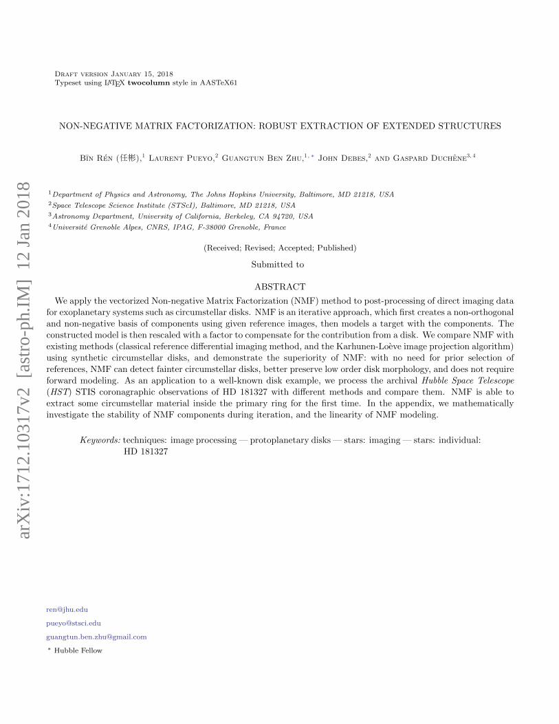
NON-NEGATIVE MATRIX FACTORIZATION: ROBUST EXTRACTION OF EXTENDED STRUCTURES

Bin Ren (任彬),1 Laurent Pueyo,2 Guangtun Ben Zhu,1, ∗ John Debes,2 and Gaspard Duchene3, 4

1Department of Physics and Astronomy, The Johns Hopkins University, Baltimore, MD 21218, USA2Space Telescope Science Institute (STScI), Baltimore, MD 21218, USA3Astronomy Department, University of California, Berkeley, CA 94720, USA4Universite Grenoble Alpes, CNRS, IPAG, F-38000 Grenoble, France

(Received; Revised; Accepted; Published)

Submitted to

ABSTRACT

We apply the vectorized Non-negative Matrix Factorization (NMF) method to post-processing of direct imaging data

for exoplanetary systems such as circumstellar disks. NMF is an iterative approach, which first creates a non-orthogonal

and non-negative basis of components using given reference images, then models a target with the components. The

constructed model is then rescaled with a factor to compensate for the contribution from a disk. We compare NMF with

existing methods (classical reference differential imaging method, and the Karhunen-Loeve image projection algorithm)

using synthetic circumstellar disks, and demonstrate the superiority of NMF: with no need for prior selection of

references, NMF can detect fainter circumstellar disks, better preserve low order disk morphology, and does not require

forward modeling. As an application to a well-known disk example, we process the archival Hubble Space Telescope

(HST) STIS coronagraphic observations of HD 181327 with different methods and compare them. NMF is able to

extract some circumstellar material inside the primary ring for the first time. In the appendix, we mathematically

investigate the stability of NMF components during iteration, and the linearity of NMF modeling.

Keywords: techniques: image processing — protoplanetary disks — stars: imaging — stars: individual:

HD 181327

ren@jhu.edu

pueyo@stsci.edu

guangtun.ben.zhu@gmail.com

∗ Hubble Fellow

arX

iv:1

712.

1031

7v2

[as

tro-

ph.I

M]

12

Jan

2018

2 Ren et al.

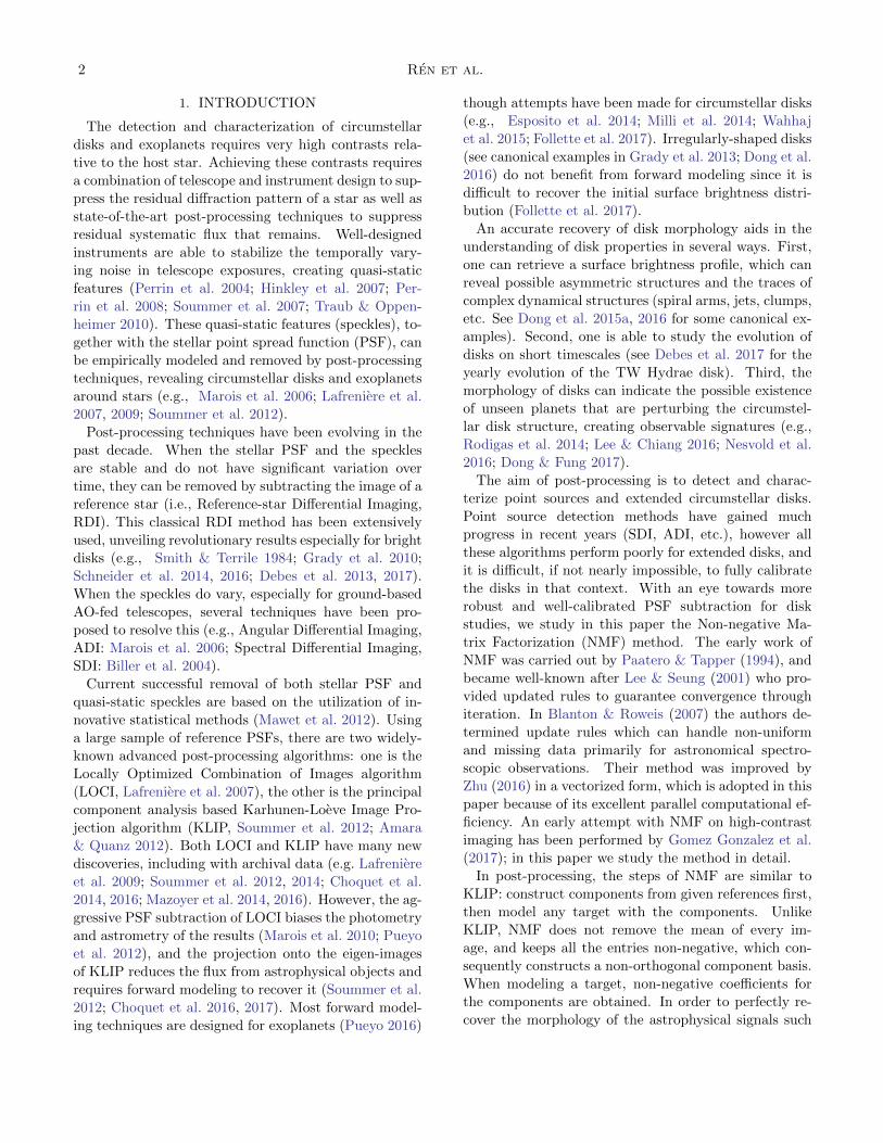
1. INTRODUCTION

The detection and characterization of circumstellar

disks and exoplanets requires very high contrasts rela-

tive to the host star. Achieving these contrasts requires

a combination of telescope and instrument design to sup-

press the residual diffraction pattern of a star as well as

state-of-the-art post-processing techniques to suppress

residual systematic flux that remains. Well-designed

instruments are able to stabilize the temporally vary-

ing noise in telescope exposures, creating quasi-static

features (Perrin et al. 2004; Hinkley et al. 2007; Per-

rin et al. 2008; Soummer et al. 2007; Traub & Oppen-

heimer 2010). These quasi-static features (speckles), to-

gether with the stellar point spread function (PSF), can

be empirically modeled and removed by post-processing

techniques, revealing circumstellar disks and exoplanets

around stars (e.g., Marois et al. 2006; Lafreniere et al.

2007, 2009; Soummer et al. 2012).

Post-processing techniques have been evolving in the

past decade. When the stellar PSF and the speckles

are stable and do not have significant variation over

time, they can be removed by subtracting the image of a

reference star (i.e., Reference-star Differential Imaging,

RDI). This classical RDI method has been extensively

used, unveiling revolutionary results especially for bright

disks (e.g., Smith & Terrile 1984; Grady et al. 2010;

Schneider et al. 2014, 2016; Debes et al. 2013, 2017).

When the speckles do vary, especially for ground-based

AO-fed telescopes, several techniques have been pro-

posed to resolve this (e.g., Angular Differential Imaging,

ADI: Marois et al. 2006; Spectral Differential Imaging,

SDI: Biller et al. 2004).

Current successful removal of both stellar PSF and

quasi-static speckles are based on the utilization of in-

novative statistical methods (Mawet et al. 2012). Using

a large sample of reference PSFs, there are two widely-

known advanced post-processing algorithms: one is the

Locally Optimized Combination of Images algorithm

(LOCI, Lafreniere et al. 2007), the other is the principal

component analysis based Karhunen-Loeve Image Pro-

jection algorithm (KLIP, Soummer et al. 2012; Amara

& Quanz 2012). Both LOCI and KLIP have many new

discoveries, including with archival data (e.g. Lafreniere

et al. 2009; Soummer et al. 2012, 2014; Choquet et al.

2014, 2016; Mazoyer et al. 2014, 2016). However, the ag-

gressive PSF subtraction of LOCI biases the photometry

and astrometry of the results (Marois et al. 2010; Pueyo

et al. 2012), and the projection onto the eigen-images

of KLIP reduces the flux from astrophysical objects and

requires forward modeling to recover it (Soummer et al.

2012; Choquet et al. 2016, 2017). Most forward model-

ing techniques are designed for exoplanets (Pueyo 2016)

though attempts have been made for circumstellar disks

(e.g., Esposito et al. 2014; Milli et al. 2014; Wahhaj

et al. 2015; Follette et al. 2017). Irregularly-shaped disks

(see canonical examples in Grady et al. 2013; Dong et al.

2016) do not benefit from forward modeling since it is

difficult to recover the initial surface brightness distri-

bution (Follette et al. 2017).

An accurate recovery of disk morphology aids in the

understanding of disk properties in several ways. First,

one can retrieve a surface brightness profile, which can

reveal possible asymmetric structures and the traces of

complex dynamical structures (spiral arms, jets, clumps,

etc. See Dong et al. 2015a, 2016 for some canonical ex-

amples). Second, one is able to study the evolution of

disks on short timescales (see Debes et al. 2017 for the

yearly evolution of the TW Hydrae disk). Third, the

morphology of disks can indicate the possible existence

of unseen planets that are perturbing the circumstel-

lar disk structure, creating observable signatures (e.g.,

Rodigas et al. 2014; Lee & Chiang 2016; Nesvold et al.

2016; Dong & Fung 2017).

The aim of post-processing is to detect and charac-

terize point sources and extended circumstellar disks.

Point source detection methods have gained much

progress in recent years (SDI, ADI, etc.), however all

these algorithms perform poorly for extended disks, and

it is difficult, if not nearly impossible, to fully calibrate

the disks in that context. With an eye towards more

robust and well-calibrated PSF subtraction for disk

studies, we study in this paper the Non-negative Ma-

trix Factorization (NMF) method. The early work of

NMF was carried out by Paatero & Tapper (1994), and

became well-known after Lee & Seung (2001) who pro-

vided updated rules to guarantee convergence through

iteration. In Blanton & Roweis (2007) the authors de-

termined update rules which can handle non-uniform

and missing data primarily for astronomical spectro-

scopic observations. Their method was improved by

Zhu (2016) in a vectorized form, which is adopted in this

paper because of its excellent parallel computational ef-

ficiency. An early attempt with NMF on high-contrast

imaging has been performed by Gomez Gonzalez et al.

(2017); in this paper we study the method in detail.

In post-processing, the steps of NMF are similar to

KLIP: construct components from given references first,

then model any target with the components. Unlike

KLIP, NMF does not remove the mean of every im-

age, and keeps all the entries non-negative, which con-

sequently constructs a non-orthogonal component basis.

When modeling a target, non-negative coefficients for

the components are obtained. In order to perfectly re-

cover the morphology of the astrophysical signals such

NMF in Direct Imaging 3

as circumstellar disks, the NMF subtraction results do

need forward modeling, however we are able to show

that, to the first order, this can be performed with a

simple search in a one-dimensional space.

The structure of this paper is as follows: §2 discusses

the limitation of current methods and explains the mech-

anism of NMF; §3 is composed of the post-processing

results of various methods with modeled disks, and the

application to a classical example of HD 181327, thus

making the NMF method standing out among current

ones; and §4 summarizes the general performance of

NMF, and discusses its significance to the field. In

the appendices, Appendix A is a list of symbols used

in this paper; Appendix B shows the update rules pro-

posed by Zhu (2016), as well as the adjustments made

for direct imaging data; Appendix C investigates the

stability of NMF components during their construction,

Appendix D presents how to model a target with the

NMF components, and Appendix E describes the our

procedure to correct for over-subtraction.

2. METHODS

To illustrate the limitation of current methods and

compare them with NMF, we took data from the HST

Space Telescope Imaging Spectrograph (STIS) corona-

graphic observations of HD 38393 (γ Leporis, Proposal

ID: 144261, PI: J. Debes), aligned the centers of the

stars using a Radon Transform-based center determina-

tion method described in Pueyo et al. (2015). We release

an improved center-determination code centerRadon2,

which is based on Radon Transform and performs line

integrals on specific parameter spaces and selected re-

gions. The code is at least 2 orders of magnitude faster

than classical Radon Transform algorithms for our STIS

data.

We cut the aligned exposures into 87×87 pixel arrays3,

corresponding with a 4.41 × 4.41 arcsec2 field of view.

The original data contains 810 0.2-second exposures of

HD 38393 at 9 different telescope orientations. In our

simulation, all the data are normalized to have flux units

of mJy arcsec−2; and to save computational time, we use

only 81 exposures by selecting just 9 exposures at each

orientation.

This section is organized as follows: §2.1 discusses the

limitation of current modeling methods, §2.2 explains

the NMF method in detail.

1 http://archive.stsci.edu/proposal_search.php?mission=

hst&id=144262 https://github.com/seawander/centerRadon.3 Note: the dimension of all the images in this paper is 87 × 87

pixels (4.41 × 4.41 arcsec2) unless otherwise specified.

2.1. Limitation of Current Methods

Current post-processing methods are excellent at find-

ing disks, but they can have disadvantages and particu-

lar limitations. We start our simulation with a synthetic

face-on disk generated by MCFOST, a radiative transfer

software to model circumstellar disks with particular

morphologies and compositions (Pinte et al. 2006, 2009).

For the exposures of HD 38393 at one orientation, the

synthetic disk was injected after being added with Pois-

son noise to simulate real observations, therefore creat-

ing the target images; while the exposures from the other

8 orientations are treated as the references.

The targets and references are then used for post-

processing. In order to perform the RDI technique, we

compute the pixel-wise median of the references, creat-

ing an empirical model of the stellar PSF and speckles,

and subtract the model from the disk-injected images.

For KLIP, we construct the components from the refer-

ences, and model the targets with the components, then

remove the KLIP model from the targets. This proce-

dure is then executed for all the 9 orientations, then the

final result is calculated from the pixel-wise median of

the 81 subtracted targets.

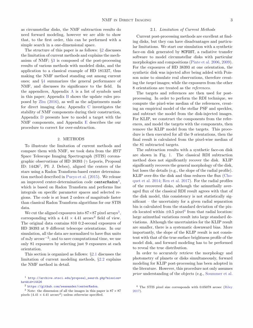
The subtraction results with a synthetic face-on disk

are shown in Fig. 1. The classical RDI subtraction

method does not significantly recover the disk. KLIP

significantly recovers the general morphology of the disk,

but loses the details (e.g., the slope of the radial profile).

KLIP over-fits the disk and thus reduces the flux (Cho-

quet et al. 2014; Ren et al. 2017). For the radial profiles

of the recovered disks, although the azimuthally aver-

aged flux of the classical RDI result agrees with that of

the disk model, this consistency is not statistically sig-

nificant – the uncertainty for a given radial separation

bin is calculated from the standard deviation of the pix-

els located within ±0.5 pixel4 from that radial location:

large azimuthal variations result into large standard de-

viations. Although the uncertainties for the KLIP result

are smaller, there is a systematic downward bias. More

importantly, the slope of the KLIP result is not consis-

tent with that of the true surface brightness profile of the

model disk, and forward modeling has to be performed

to reveal the true distribution.

In order to accurately retrieve the morphology and

photometry of planets or disks simultaneously, forward

modeling for KLIP post-processing has been adopted in

the literature. However, this procedure not only assumes

prior understanding of the objects (e.g., Soummer et al.

4 The STIS pixel size corresponds with 0.05078 arcsec (Riley2017).

4 Ren et al.

1 arcsec9 AU

Figure 1. Demonstration of limitations to current PSF sub-traction methods using a synthetic face-on circumstellar diskwith integrated flux ratio Fdisk/Fstar = 7.4× 10−6. (a) TheHST-STIS exposures of HD 38393 added with a syntheticface-on disk and no PSF subtraction. The disk is unseendue to its faintness relative to the wings of the stellar PSF,and the central dark region is the coronagraphic BAR5 maskof STIS. (b) Classical RDI subtraction result: the north-eastern region shows an over-luminosity which does not be-long to the disk. (c) Subtraction result with KLIP: the diskis seen but its flux is reduced and its morphology modified.(d) Radial surface brightness profiles of the subtraction re-sults and the disk model. While the profile with the classicalmethod agrees with the disk model, the disk is not signifi-cantly detected in this region due to large systematic PSFsubtraction residuals. KLIP is unable to recover the true ra-dial profile, introducing unphysically negative pixels to thesurface brightness distribution. See Fig. 8 for the disk model,and the subtraction result with NMF.

2012; Wahhaj et al. 2015; Pueyo 2016), it is also time-

consuming to iteratively recover the likely disk surface

brightness distribution (e.g., Choquet et al. 2016, 2017).

2.2. Non-negative Matrix Factorization (NMF)

The methods to faithfully recover astrophysical ob-

jects with high contrast imaging techniques has been

evolving. On one hand, new methods have been pro-

posed and studied to minimize over-subtraction: Pueyo

et al. (2012) focuses on the positive coefficients for the

LOCI method, and substantially improves the charac-

terization quality of point source spectra. On the other

hand, forward modeling is introduced as a correction

method for the reduced data: Wahhaj et al. (2015)

assumes a prior model of disks for LOCI subtraction.

Pueyo (2016) takes the instrumental PSF to character-

ize point sources with the KLIP method. Current for-

ward modeling attempts are best optimized for planet

characterization, while for extended and resolved objects

like circumstellar disks, assumptions of disk morphology

have to be made. These assumptions may not accurately

recover the true flux, particularly for disks that deviate

from simple morphologies. In this paper, we aim to

circumvent the forward modeling difficulties by study-

ing a new method – Non-negative Matrix Factorization

(NMF).

NMF decomposes a matrix into the product of two

non-negative ones (Paatero & Tapper 1994; Lee & Se-

ung 2001), a technique that has been used over the past

decade to account for astrophysical problems (Blanton

& Roweis 2007; Zhu 2016). Inspired by the Pueyo et al.

(2012) work of adopting positive coefficients, we study

NMF because of its non-negativity, which is well suited

for astrophysical direct imaging observations. The pre-

vious applications of NMF are to one-dimensional as-

trophysical spectra. Two-dimensional images have sig-

nificantly larger amounts of information and therefore

escalate the computational cost. In order to make this

problem computationally tractable we make the follow-

ing adjustments: we flatten every image into a one-

dimensional array to maximize the utilization of cur-

rently available tools and we adopt the vectorized NMF

technique (Zhu 2016, NonnegMFPy5) to implement par-

allel computation with multiple cores.

The NMF application to imaging data is comprised of

three steps: constructing the basis of components with

the reference images (§2.2.1), modeling any new target

with the component basis (§2.2.2), and correcting for the

over-fitting with a scaling factor (§2.2.3). We release ourversion of NMF 6, which is also available in the pyKLIP

package (Wang et al. 2015).

2.2.1. Component Construction

The first step of NMF is to approximate the refer-

ence matrix R, with the product of two non-negative

matrices: the coefficient matrix W , and the component

matrix H, i.e.,

R ≈WH, (1)

by minimizing their Euclidean distances, see Ap-

pendix A for detailed definition of symbols. The ap-

proximation of Eq. (1) is guaranteed to converge with

5 https://github.com/guangtunbenzhu/NonnegMFPy6 https://github.com/seawander/nmf_imaging

NMF in Direct Imaging 5

iteration rules in Zhu (2016) using:

W (k+1) = W (k) ◦ RH(k)T

W (k)H(k)H(k)T, (2)

H(k+1) = H(k) ◦ W (k)TR

W (k)TW (k)H(k), (3)

with random initializations. In the above equations, the

circle ◦ and fraction bar7 (··· )(··· ) denote element-wise mul-

tiplication and division for matrices, the superscripts

enclosed with (·) denote iteration steps, and the super-

script T stands for matrix transposition. For astronomi-

cal data, a weighting function V , which is usually the el-

ementwise variance (i.e., the square of the uncertainties)

of R, is applied to weigh the contribution from different

pixels and take care of heteroskedastic data (Blanton &

Roweis 2007; Zhu 2016), see Appendix B for the adap-

tation for our STIS imaging data.

The connection between NMF and previous statisti-

cal methods can be illustrated using Eq. (2): we can

cross out the W terms on the righthand side8, and get

W = RHT

HHT , which stands for the projection of vector R

onto vector H. This expression is in essence performing

least square estimation as in KLIP, where the inversion

of the covariance matrix of the components is required

(i.e., the inverse of HHT ), however the covariance ma-

trices are often poorly conditioned for inversion. Intu-

itively, NMF returns a non-negative approximation of

the matrix inverse through iteration.

In the KLIP method, the importance of the compo-

nents is ranked based on the magnitude of their corre-

sponding eigenvalues. For NMF we rank them by con-

structing the components sequentially: with n compo-

nents constructed we construct the (n + 1)-th compo-

nent using the n previously constructed ones. In our

construction we only randomize the initialization of the

(n+ 1)-th component, while the first n components are

initialized with their previously constructed values. See

Appendix C for detailed expression and derivation. This

construction method not only ranks the components,

but also is essential for the linearity in target modeling

in the next subsection.

2.2.2. Target Modeling (“Projection”)

The sequential construction of NMF components is

the foundation of this paper. First, as illustrated in Ap-

pendix C, the components remain stable in this setup.

Second, the stability of the components guarantees a lin-

ear separation of the disk signal from the stellar signals

7 Note: all the fraction bars in this paper are element-wisedivision of matrices unless otherwise specified

8 Note: this operation is for demonstration purpose only, it isnot mathematically practical.

(Appendix D). Third and most importantly, the linear-

ity of the target modeling process allows for our attempt

to circumvent forward modeling with a scaling factor, as

illustrated in Appendix E.

With the basis of NMF components constructed se-

quentially, the next step is to model the targets with

the components. For a flattened target T , we now min-

imize ||T − ωH||2 with an iteration rule9

ω(k+1) = ω(k) ◦ THT

ω(k)HHT, (4)

where ω is the 1 × n coefficient matrix for the target,

and H is the NMF components constructed in the previ-

ous paragraph. This expression is essentially performing

least square approximation as in KLIP, but the coeffi-

cients are smaller in magnitude (Appendix D). A more

detailed expression taking weighting function into ac-

count is given by Zhu (2016) and the adaptation to our

STIS data is shown in Appendix B. When the above

process converges, the NMF model of the target can be

represented by

TNMF = ωH. (5)

2.2.3. Disk Retrieval via “Forward Modelling”

With sequentially constructed components, the tar-

get modeling procedure is able to linearly separate the

circumstellar disk from the others, as illustrated in

Eq. (D42). To first order, we have

TNMF = DNMF + SNMF, (6)

where the subscript NMF means performing the NMF

modeling result for the stellar signal (S) or disk signal

(D) alone. In addition, when we sequentially model the

target, if the disk does not resemble any NMF compo-

nent, then the first component, which explains ∼ 90%

of the residual noise (shown in §3.1.1), will always dom-

inate the modeling for the disk – the captured morphol-

ogy of the disk is just another copy of the NMF model

of the stellar PSF and the speckles (shown in §3.1.2),

i.e.,

DNMF ≈ αSNMF, (7)

where α is a positive number.

The way to correct for the contribution from the disk

is to introduce a scaling factor f , which satisfies

fTNMF = SNMF, (8)

then when we subtract the scaled NMF model of the tar-

get from the raw exposure, we will have the disk image:

T − fTNMF = T − SNMF = D. (9)

9 This rule is the one dimensional case of Eq. (2).

6 Ren et al.

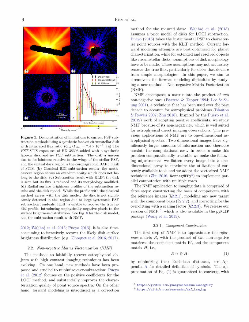
Ideally, we will solve for f = 1/(1 +α), however since α

is not known, we have to find f empirically.

9 AU1 arcsec

Figure 2. Illustration of the scaling factor for the disk modelin Fig. 5. (a): Face-on disk model created by MCFOST. (b):Scaled reduced disk with f = 0.930. There are PSF residualssince the scaling factor is smaller than the optimum one.(c): Scaled reduced disk with f = f = 0.982, the best diskcorresponding with the optimal scaling factor obtained fromthe BFF procedure. (d): Reduced disk with no correction(i.e., f = 1). The disk flux is reduced due to oversubtraction,and pixels beyond the outskirts of the disk are all negative.See Fig. 3 for a comparison of the radial profiles.

We introduce the Best Factor Finding (BFF) proce-

dure in Appendix E as our attempt to circumvent for-

ward modeling with a simple scaling factor that mini-

mizes the corresponding background noise. To illustrate

the efficiency of BFF, we show our results in the STIS

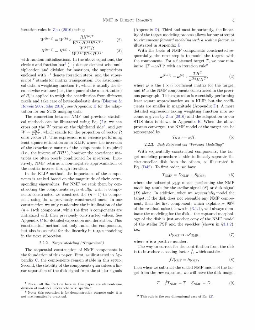
data with different scaling factors in Fig. 2 and Fig. 3.

When we do not know the existence of the astrophysical

signal (i.e., the disk) a priori, the residual variance de-

pendence on scaling factor agrees consistently with the

dependence of the Euclidean distances between the re-

duction results (Df ’s) and the true model (D) on the

scaling factor. This consistency has been observed for

synthetic disks at different inclination angles in our sim-

ulation, which is not shown in this paper to avoid re-

dundancy of figures.

We could use multiple scaling factors to rescale every

over-fitting component, and BFF will work for compo-

nents that are affecting the overall morphology. Given

0.90 0.92 0.94 0.96 0.98 1.00

Scaling Factor f

101

102

103

104

105

Valu

es

Noise Variance

Euclidean Distance

0.4 0.6 0.8 1.0 1.2 1.4

Radial Separation (arcsec)

100

0

100

200

300

400

Flux (

mJy

arc

sec−

2)

ModelD0. 93

D

D1

Figure 3. (a) The curve for Euclidean distance between thescaled disks and the MCFOST model in Figs. 5 and 2 (dash-dotted blue line) is consistent with the curve for the back-ground noise (dashed black line). This is the demonstrationof the effectiveness of the BFF procedure. (b) Radial profilesfor the model (black solid line), and scaled disks with threedifferent scaling levels. When f = 0.930 < f , the radial pro-file (black solid line) is moving upwards in relative to thatof the model; when f = 0.982 = f , its radial profile (dottedyellow line) agrees with that of the model; for f = 1 > f , thediskless pixels are all negative (blue dash-dotted line, com-pare with the gray dashed horizontal line of 0’s). See Fig. 6for the results from other methods.

the sparseness of the NMF coefficients (ωD, §3.1.2), this

is easily achievable with a grid search. However, we only

focus on the first component, since the BFF procedureis trying to optimize the whole field of view, while the

components of higher order usually do not have much

influence in our simulations.

3. COMPARISON AND APPLICATION

In the previous section we have demonstrated the lim-

itation of current methods and the mechanism of NMF.

In this section, we aim to demonstrate the ability of

NMF in direct imaging using specific examples: we first

compare the statistical properties of NMF and KLIP,

as well as the intermediate steps of them in §3.1, then

focus on the post-processing results. We compare the

NMF results with that of the classical RDI and KLIP

subtraction methods using synthetic disks in §3.2. In

§3.3 we focus on a well-known example as a sanity check

of NMF: applying the method to the HST -STIS coron-

agraphic imaging observations of HD 181327.

NMF in Direct Imaging 7

3.1. NMF vs KLIP: Statistical Properties &

Intermediate Steps

In this subsection, we aim to address the statistical

differences and intermediate steps between NMF and

KLIP, and investigate why the non-negativity of NMF

can yield better results. Noise and disk signal are the

two constituents in a target image. However, they are

always correlated with each other and separating them

is the goal of all post-processing efforts. In the target

modeling process, we aim to maximize noise removal and

minimize disk flux removal. We therefore compare NMF

with KLIP in these two aspects.

3.1.1. Noise Removal

Removing the quasi-static noise from the observations

is the most fundamental procedure in post-processing.

With the 81 STIS images of HD 38393, we calculate the

Fractional Residual Variance (FRV) curves in the fol-

lowing way (Fig. 1 of Soummer et al. 2012). For each

image we cumulatively increase the number of compo-

nents and model it with KLIP or NMF, then subtract

the model from the image to obtain the residual image.

Finally the FRV is calculated by dividing the variance

of the residual image by that of the original image. The

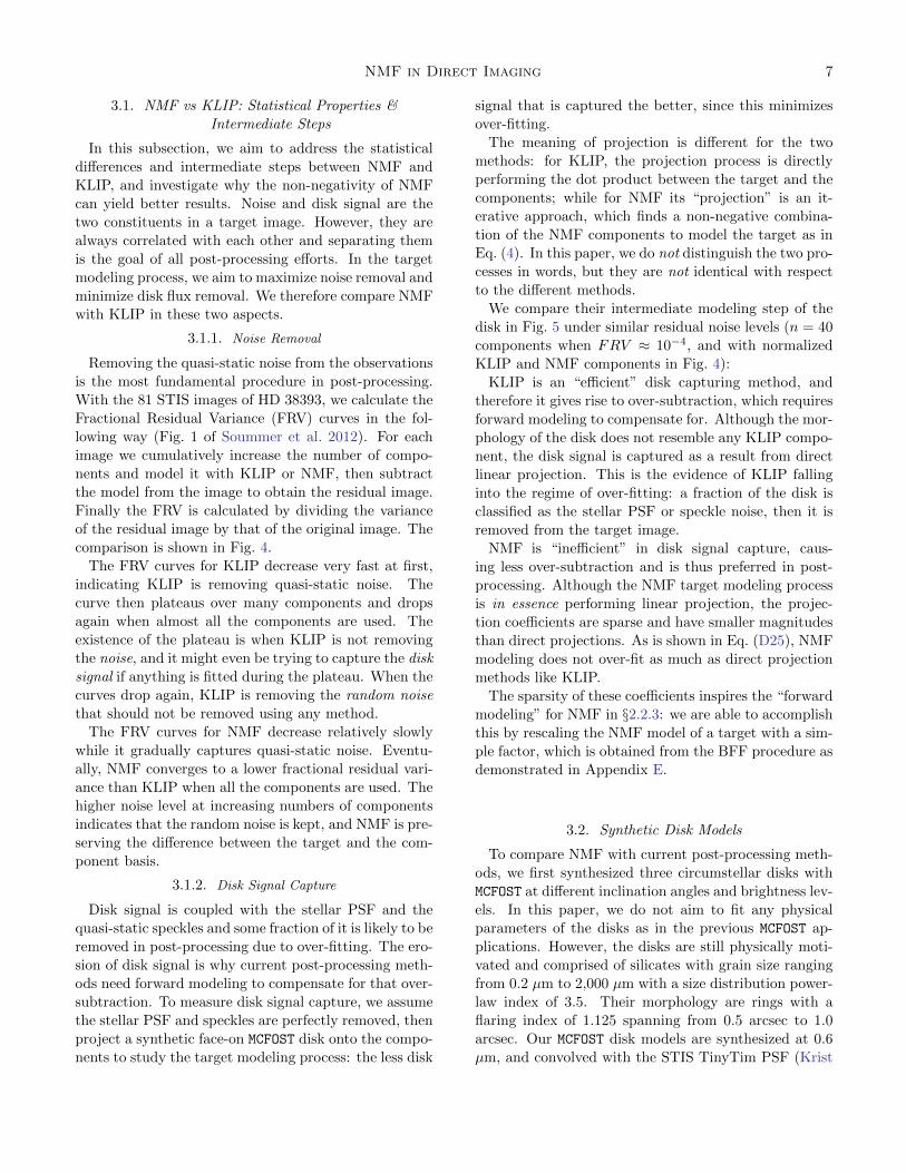
comparison is shown in Fig. 4.

The FRV curves for KLIP decrease very fast at first,

indicating KLIP is removing quasi-static noise. The

curve then plateaus over many components and drops

again when almost all the components are used. The

existence of the plateau is when KLIP is not removing

the noise, and it might even be trying to capture the disk

signal if anything is fitted during the plateau. When the

curves drop again, KLIP is removing the random noise

that should not be removed using any method.

The FRV curves for NMF decrease relatively slowly

while it gradually captures quasi-static noise. Eventu-

ally, NMF converges to a lower fractional residual vari-

ance than KLIP when all the components are used. The

higher noise level at increasing numbers of components

indicates that the random noise is kept, and NMF is pre-

serving the difference between the target and the com-

ponent basis.

3.1.2. Disk Signal Capture

Disk signal is coupled with the stellar PSF and the

quasi-static speckles and some fraction of it is likely to be

removed in post-processing due to over-fitting. The ero-

sion of disk signal is why current post-processing meth-

ods need forward modeling to compensate for that over-

subtraction. To measure disk signal capture, we assume

the stellar PSF and speckles are perfectly removed, then

project a synthetic face-on MCFOST disk onto the compo-

nents to study the target modeling process: the less disk

signal that is captured the better, since this minimizes

over-fitting.

The meaning of projection is different for the two

methods: for KLIP, the projection process is directly

performing the dot product between the target and the

components; while for NMF its “projection” is an it-

erative approach, which finds a non-negative combina-

tion of the NMF components to model the target as in

Eq. (4). In this paper, we do not distinguish the two pro-

cesses in words, but they are not identical with respect

to the different methods.

We compare their intermediate modeling step of the

disk in Fig. 5 under similar residual noise levels (n = 40

components when FRV ≈ 10−4, and with normalized

KLIP and NMF components in Fig. 4):

KLIP is an “efficient” disk capturing method, and

therefore it gives rise to over-subtraction, which requires

forward modeling to compensate for. Although the mor-

phology of the disk does not resemble any KLIP compo-

nent, the disk signal is captured as a result from direct

linear projection. This is the evidence of KLIP falling

into the regime of over-fitting: a fraction of the disk is

classified as the stellar PSF or speckle noise, then it is

removed from the target image.

NMF is “inefficient” in disk signal capture, caus-

ing less over-subtraction and is thus preferred in post-

processing. Although the NMF target modeling process

is in essence performing linear projection, the projec-

tion coefficients are sparse and have smaller magnitudes

than direct projections. As is shown in Eq. (D25), NMF

modeling does not over-fit as much as direct projection

methods like KLIP.

The sparsity of these coefficients inspires the “forward

modeling” for NMF in §2.2.3: we are able to accomplish

this by rescaling the NMF model of a target with a sim-

ple factor, which is obtained from the BFF procedure as

demonstrated in Appendix E.

3.2. Synthetic Disk Models

To compare NMF with current post-processing meth-

ods, we first synthesized three circumstellar disks with

MCFOST at different inclination angles and brightness lev-

els. In this paper, we do not aim to fit any physical

parameters of the disks as in the previous MCFOST ap-

plications. However, the disks are still physically moti-

vated and comprised of silicates with grain size ranging

from 0.2 µm to 2,000 µm with a size distribution power-

law index of 3.5. Their morphology are rings with a

flaring index of 1.125 spanning from 0.5 arcsec to 1.0

arcsec. Our MCFOST disk models are synthesized at 0.6

µm, and convolved with the STIS TinyTim PSF (Krist

8 Ren et al.

0 10 20 30 40 50 60 70 80

Number of Components

10-8

10-7

10-6

10-5

10-4

10-3

10-2

10-1

100

Fract

ional R

esi

dual V

ari

ance

KLIP

KLIP theory

0 10 20 30 40 50 60 70 80

Number of Components

10-8

10-7

10-6

10-5

10-4

10-3

10-2

10-1

100

Fract

ional R

esi

dual V

ari

ance

NMF

Figure 4. FRV as a function of the number of components. (a): FRV plots for KLIP, the gray solid lines are that for individualimages, the blue solid line is the theoretical curve (as in Fig. 1 of Soummer et al. 2012). The existence of the plateau fromn ≈ 10 to n ≈ 60 indicates that KLIP is not efficiently capturing noise over those components. (b): FRV plots for NMF, thegray dashed lines are for individual images. There is no plateau in the NMF reduction, indicating it continues capture noisewhen we increase the number of components. The comparison between KLIP and NMF projections at similar FRV levels isshown in Fig. 5. Note: The FRV trends of KLIP and NMF are not limited to the STIS data studied in this paper, and shouldbe applicable to all other instruments.

et al. 2011)10, to simulate the HST-STIS response: at

this wavelength, the incident photons from the host star

are scattered by the disks and then received by the tele-

scopes.

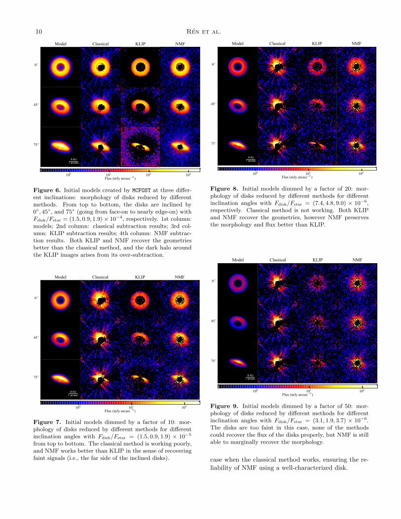
We reduced the synthetic disks in the same manner as

in §2.1 with the classical RDI, KLIP, and NMF meth-

ods. The face-on disk spanning from 0.5 arcsec to 1.0

arcsec in Fig. 5 is adopted as the initial model. We

then inclined the model disk at 45◦ and 75◦ to verify

performance for differing inclination angles. To investi-

gate the performance of the three methods at different

contrasts Fig. 6 shows comparisons for disks divided by

factors of 10, 20, and 50, which is equivalent to reducing

disk mass. The disks’ Fdisk/Fstar range from ∼ 10−4 to

∼ 10−6. The morphology results are shown in Figs. 6,

7, 8, and 9, respectively.

3.2.1. Morphology

Morphology probes the spatial distribution of the cir-

cumstellar material, which should be recovered as close

to the photon noise limit as possible. From the mor-

phology results for different disks and brightness levels

in Figs. 6 – 9, we compare the three methods as follows:

Classical subtraction is only able to recover the

morphology of the face-on disk in the brightest cases

10 http://www.stsci.edu/hst/observatory/focus/TinyTim

(Fdisk/Fstar ∼ 10−4), it cannot recover the dimmer

ones.

KLIP is able to recover the general morphology of the

disks in all cases, however the disk fluxes are reduced

due to its systematic over-fitting bias (§3.1.2), therefore

forward modeling is needed to recover the real morphol-

ogy of the disks. Moreover, for detailed structures, es-

pecially when the dynamic range is large, KLIP will lose

the relatively faint information due to mean-subtraction

(see the disappearance of the far side in the lower regions

of the inclined disks in Figs. 6 – 9).

NMF outperforms other methods not only in recover-

ing the morphology of the disks, but also in recovering

the faint structure: the faint far side of the inclined disks

is recovered in the results.

When the disks are too faint (Fig. 9), the reduced

results are dominated by random noise, and none of the

methods but NMF could marginally recover the mor-

phology of the disks.

For a quantitative comparison of the three methods,

we compute the χ2 values using the initial model and

the results in this subsection. To better illustrate the

relative goodness of recovery, we plot the χ2 ratios be-

tween different methods and the classical RDI method in

Fig. 10. NMF performs better than the classical method

in this way; when comparing with KLIP, NMF is able

NMF in Direct Imaging 9

Projection ontoKLIP components

Projection ontoNMF components

KLIP coefficients

NMF coefficients9 AU

1 arcsecsparse

Figure 5. Comparison between KLIP and NMF projections using a synthetic face-on MCFOST disk model. (a) The disk model.(b) The projection of the disk model onto the KLIP components, the central circularly-shaped structure is the result fromover-fitting. (c) The coefficients of each component in KLIP modeling. (d) The “projection” of the model onto the NMFcomponents. (e) The coefficients of each component in NMF modeling in (d): the fact that both the components and thecoefficients are non-negative reduces the likelihood of over-fitting, as shown in Eq. (D25). Note: the central dark regions in (b)and (d) are the coronagraphic occulting mask at the STIS BAR5 position; and the images are in the same scale.

reach lower or similar levels, demonstrating its compe-

tence in disk retrieval. In the cases when the NMF χ2

values are slightly larger than that of KLIP, it is from the

fact that KLIP is over-fitting the random noise, which

in principle should not be fitted by any method, rather

than KLIP has a better matching to the disk model.

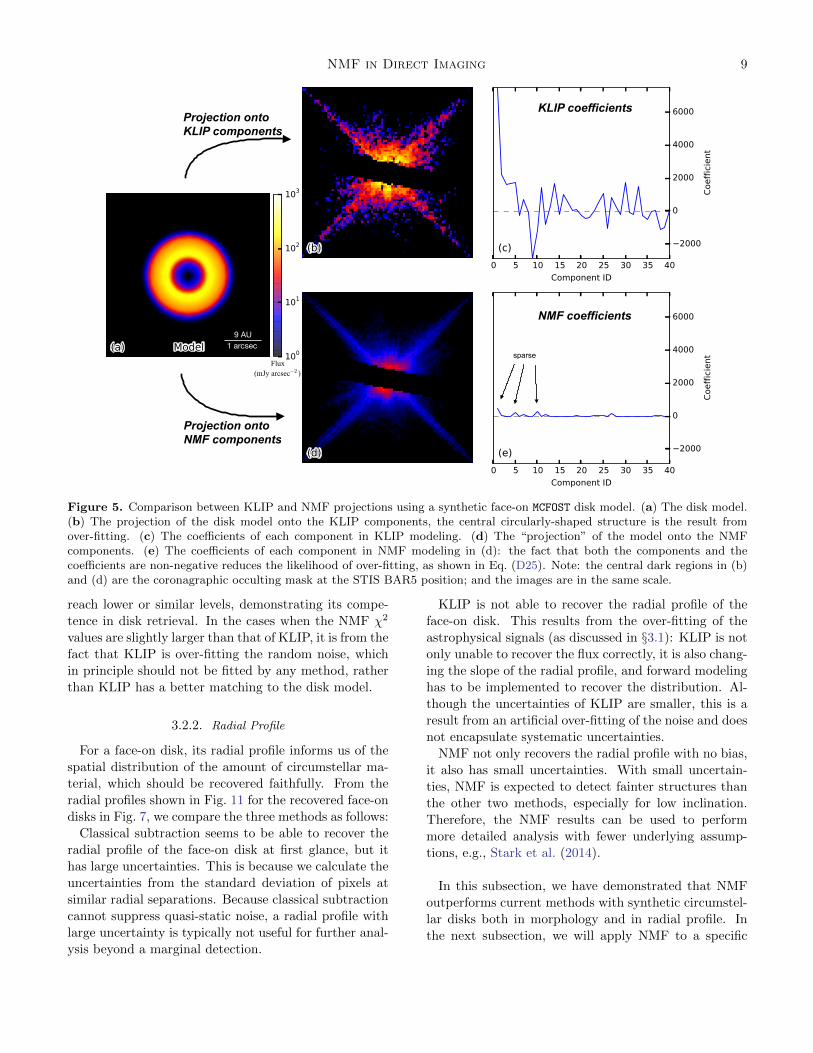
3.2.2. Radial Profile

For a face-on disk, its radial profile informs us of the

spatial distribution of the amount of circumstellar ma-

terial, which should be recovered faithfully. From the

radial profiles shown in Fig. 11 for the recovered face-on

disks in Fig. 7, we compare the three methods as follows:

Classical subtraction seems to be able to recover the

radial profile of the face-on disk at first glance, but it

has large uncertainties. This is because we calculate the

uncertainties from the standard deviation of pixels at

similar radial separations. Because classical subtraction

cannot suppress quasi-static noise, a radial profile with

large uncertainty is typically not useful for further anal-

ysis beyond a marginal detection.

KLIP is not able to recover the radial profile of the

face-on disk. This results from the over-fitting of the

astrophysical signals (as discussed in §3.1): KLIP is not

only unable to recover the flux correctly, it is also chang-

ing the slope of the radial profile, and forward modelinghas to be implemented to recover the distribution. Al-

though the uncertainties of KLIP are smaller, this is a

result from an artificial over-fitting of the noise and does

not encapsulate systematic uncertainties.

NMF not only recovers the radial profile with no bias,

it also has small uncertainties. With small uncertain-

ties, NMF is expected to detect fainter structures than

the other two methods, especially for low inclination.

Therefore, the NMF results can be used to perform

more detailed analysis with fewer underlying assump-

tions, e.g., Stark et al. (2014).

In this subsection, we have demonstrated that NMF

outperforms current methods with synthetic circumstel-

lar disks both in morphology and in radial profile. In

the next subsection, we will apply NMF to a specific

10 Ren et al.

9 AU1 arcsec

Figure 6. Initial models created by MCFOST at three differ-ent inclinations: morphology of disks reduced by differentmethods. From top to bottom, the disks are inclined by0◦, 45◦, and 75◦ (going from face-on to nearly edge-on) withFdisk/Fstar = (1.5, 0.9, 1.9)× 10−4, respectively. 1st column:models; 2nd column: classical subtraction results; 3rd col-umn: KLIP subtraction results; 4th column: NMF subtrac-tion results. Both KLIP and NMF recover the geometriesbetter than the classical method, and the dark halo aroundthe KLIP images arises from its over-subtraction.

9 AU1 arcsec

Figure 7. Initial models dimmed by a factor of 10: mor-phology of disks reduced by different methods for differentinclination angles with Fdisk/Fstar = (1.5, 0.9, 1.9) × 10−5

from top to bottom. The classical method is working poorly,and NMF works better than KLIP in the sense of recoveringfaint signals (i.e., the far side of the inclined disks).

9 AU1 arcsec

Figure 8. Initial models dimmed by a factor of 20: mor-phology of disks reduced by different methods for differentinclination angles with Fdisk/Fstar = (7.4, 4.8, 9.0) × 10−6,respectively. Classical method is not working. Both KLIPand NMF recover the geometries, however NMF preservesthe morphology and flux better than KLIP.

9 AU1 arcsec

Figure 9. Initial models dimmed by a factor of 50: mor-phology of disks reduced by different methods for differentinclination angles with Fdisk/Fstar = (3.1, 1.9, 3.7) × 10−6.The disks are too faint in this case, none of the methodscould recover the flux of the disks properly, but NMF is stillable to marginally recover the morphology.

case when the classical method works, ensuring the re-

liability of NMF using a well-characterized disk.

NMF in Direct Imaging 11

Classical KLIP NMF

10 2

10 1

100

101

2 Met

hod/

2 Clas

sical

dimming = 1dimming = 10dimming = 20dimming = 50

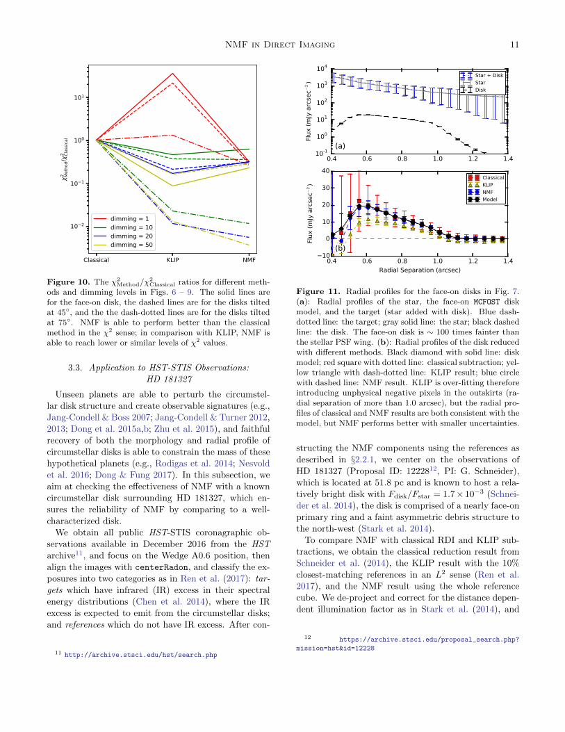
Figure 10. The χ2Method/χ

2Classical ratios for different meth-

ods and dimming levels in Figs. 6 – 9. The solid lines arefor the face-on disk, the dashed lines are for the disks tiltedat 45◦, and the the dash-dotted lines are for the disks tiltedat 75◦. NMF is able to perform better than the classicalmethod in the χ2 sense; in comparison with KLIP, NMF isable to reach lower or similar levels of χ2 values.

3.3. Application to HST-STIS Observations:

HD 181327

Unseen planets are able to perturb the circumstel-

lar disk structure and create observable signatures (e.g.,

Jang-Condell & Boss 2007; Jang-Condell & Turner 2012,

2013; Dong et al. 2015a,b; Zhu et al. 2015), and faithful

recovery of both the morphology and radial profile of

circumstellar disks is able to constrain the mass of these

hypothetical planets (e.g., Rodigas et al. 2014; Nesvoldet al. 2016; Dong & Fung 2017). In this subsection, we

aim at checking the effectiveness of NMF with a known

circumstellar disk surrounding HD 181327, which en-

sures the reliability of NMF by comparing to a well-

characterized disk.

We obtain all public HST-STIS coronagraphic ob-

servations available in December 2016 from the HST

archive11, and focus on the Wedge A0.6 position, then

align the images with centerRadon, and classify the ex-

posures into two categories as in Ren et al. (2017): tar-

gets which have infrared (IR) excess in their spectral

energy distributions (Chen et al. 2014), where the IR

excess is expected to emit from the circumstellar disks;

and references which do not have IR excess. After con-

11 http://archive.stsci.edu/hst/search.php

0.4 0.6 0.8 1.0 1.2 1.410-1

100

101

102

103

104

Flux (

mJy

arc

sec−

2)

Star + Disk

Star

Disk

0.4 0.6 0.8 1.0 1.2 1.4

Radial Separation (arcsec)

10

0

10

20

30

40

Flux (

mJy

arc

sec−

2)

Classical

KLIP

NMF

Model

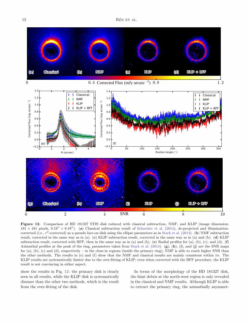
Figure 11. Radial profiles for the face-on disks in Fig. 7.(a): Radial profiles of the star, the face-on MCFOST diskmodel, and the target (star added with disk). Blue dash-dotted line: the target; gray solid line: the star; black dashedline: the disk. The face-on disk is ∼ 100 times fainter thanthe stellar PSF wing. (b): Radial profiles of the disk reducedwith different methods. Black diamond with solid line: diskmodel; red square with dotted line: classical subtraction; yel-low triangle with dash-dotted line: KLIP result; blue circlewith dashed line: NMF result. KLIP is over-fitting thereforeintroducing unphysical negative pixels in the outskirts (ra-dial separation of more than 1.0 arcsec), but the radial pro-files of classical and NMF results are both consistent with themodel, but NMF performs better with smaller uncertainties.

structing the NMF components using the references as

described in §2.2.1, we center on the observations of

HD 181327 (Proposal ID: 1222812, PI: G. Schneider),

which is located at 51.8 pc and is known to host a rela-

tively bright disk with Fdisk/Fstar = 1.7× 10−3 (Schnei-

der et al. 2014), the disk is comprised of a nearly face-on

primary ring and a faint asymmetric debris structure to

the north-west (Stark et al. 2014).

To compare NMF with classical RDI and KLIP sub-

tractions, we obtain the classical reduction result from

Schneider et al. (2014), the KLIP result with the 10%

closest-matching references in an L2 sense (Ren et al.

2017), and the NMF result using the whole reference

cube. We de-project and correct for the distance depen-

dent illumination factor as in Stark et al. (2014), and

12 https://archive.stsci.edu/proposal_search.php?

mission=hst&id=12228

12 Ren et al.

0 0. 4 0. 8 1. 2Corrected Flux (mJy arcsec−2)

0 1 2 3 4

R (arcsec)

0.2

0.0

0.2

0.4

0.6

0.8

1.0

1.2

1.4

Corr

ect

ed F

lux (

mJy

arc

sec−

2)

Classical

NMF

KLIP

KLIP + BFF

0 50 100 150 200 250 300 350

Position Angle ( ◦ )

0.2

0.0

0.2

0.4

0.6

0.8

1.0

1.2

1.4

Corr

ect

ed F

lux (

mJy

arc

sec−

2)

Classical

NMF

KLIP

KLIP + BFF

0 2 4 6 8 10SNR

Figure 12. Comparison of HD 181327 STIS disk reduced with classical subtraction, NMF, and KLIP (image dimension:181 × 181 pixels, 9.18′′ × 9.18′′). (a) Classical subtraction result of Schneider et al. (2014), de-projected and illumination-corrected (i.e., r2-corrected) as a pseudo face-on disk using the ellipse parameters as in Stark et al. (2014). (b) NMF subtractionresult, corrected in the same way as in (a). (c) KLIP subtraction result, corrected in the same way as in (a) and (b). (d) KLIPsubtraction result, corrected with BFF, then in the same way as in (a) and (b). (e) Radial profiles for (a), (b), (c), and (d). (f)Azimuthal profiles at the peak of the ring, parameters taken from Stark et al. (2014). (g), (h), (i), and (j) are the SNR mapsfor (a), (b), (c) and (d), respectively – in the close-in regions (inside the primary ring), NMF is able to reach higher SNR thanthe other methods. The results in (e) and (f) show that the NMF and classical results are mainly consistent within 1σ. TheKLIP results are systematically fainter due to the over-fitting of KLIP; even when corrected with the BFF procedure, the KLIPresult is not convincing in either aspect.

show the results in Fig. 12: the primary disk is clearly

seen in all results, while the KLIP disk is systematically

dimmer than the other two methods, which is the result

from the over-fitting of the disk.

In terms of the morphology of the HD 181327 disk,

the faint debris at the north-west region is only revealed

in the classical and NMF results. Although KLIP is able

to extract the primary ring, the azimuthally asymmet-

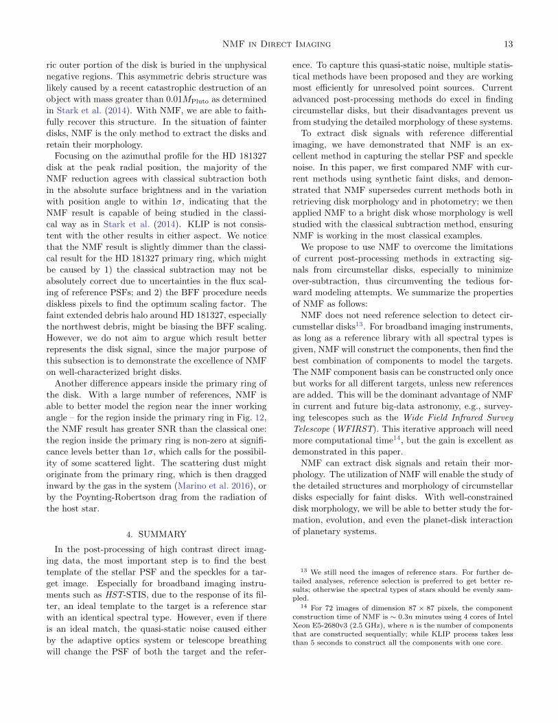
NMF in Direct Imaging 13

ric outer portion of the disk is buried in the unphysical

negative regions. This asymmetric debris structure was

likely caused by a recent catastrophic destruction of an

object with mass greater than 0.01MPluto as determined

in Stark et al. (2014). With NMF, we are able to faith-

fully recover this structure. In the situation of fainter

disks, NMF is the only method to extract the disks and

retain their morphology.

Focusing on the azimuthal profile for the HD 181327

disk at the peak radial position, the majority of the

NMF reduction agrees with classical subtraction both

in the absolute surface brightness and in the variation

with position angle to within 1σ, indicating that the

NMF result is capable of being studied in the classi-

cal way as in Stark et al. (2014). KLIP is not consis-

tent with the other results in either aspect. We notice

that the NMF result is slightly dimmer than the classi-

cal result for the HD 181327 primary ring, which might

be caused by 1) the classical subtraction may not be

absolutely correct due to uncertainties in the flux scal-

ing of reference PSFs; and 2) the BFF procedure needs

diskless pixels to find the optimum scaling factor. The

faint extended debris halo around HD 181327, especially

the northwest debris, might be biasing the BFF scaling.

However, we do not aim to argue which result better

represents the disk signal, since the major purpose of

this subsection is to demonstrate the excellence of NMF

on well-characterized bright disks.

Another difference appears inside the primary ring of

the disk. With a large number of references, NMF is

able to better model the region near the inner working

angle – for the region inside the primary ring in Fig. 12,

the NMF result has greater SNR than the classical one:

the region inside the primary ring is non-zero at signifi-

cance levels better than 1σ, which calls for the possibil-

ity of some scattered light. The scattering dust might

originate from the primary ring, which is then dragged

inward by the gas in the system (Marino et al. 2016), or

by the Poynting-Robertson drag from the radiation of

the host star.

4. SUMMARY

In the post-processing of high contrast direct imag-

ing data, the most important step is to find the best

template of the stellar PSF and the speckles for a tar-

get image. Especially for broadband imaging instru-

ments such as HST-STIS, due to the response of its fil-

ter, an ideal template to the target is a reference star

with an identical spectral type. However, even if there

is an ideal match, the quasi-static noise caused either

by the adaptive optics system or telescope breathing

will change the PSF of both the target and the refer-

ence. To capture this quasi-static noise, multiple statis-

tical methods have been proposed and they are working

most efficiently for unresolved point sources. Current

advanced post-processing methods do excel in finding

circumstellar disks, but their disadvantages prevent us

from studying the detailed morphology of these systems.

To extract disk signals with reference differential

imaging, we have demonstrated that NMF is an ex-

cellent method in capturing the stellar PSF and speckle

noise. In this paper, we first compared NMF with cur-

rent methods using synthetic faint disks, and demon-

strated that NMF supersedes current methods both in

retrieving disk morphology and in photometry; we then

applied NMF to a bright disk whose morphology is well

studied with the classical subtraction method, ensuring

NMF is working in the most classical examples.

We propose to use NMF to overcome the limitations

of current post-processing methods in extracting sig-

nals from circumstellar disks, especially to minimize

over-subtraction, thus circumventing the tedious for-

ward modeling attempts. We summarize the properties

of NMF as follows:

NMF does not need reference selection to detect cir-

cumstellar disks13. For broadband imaging instruments,

as long as a reference library with all spectral types is

given, NMF will construct the components, then find the

best combination of components to model the targets.

The NMF component basis can be constructed only once

but works for all different targets, unless new references

are added. This will be the dominant advantage of NMF

in current and future big-data astronomy, e.g., survey-

ing telescopes such as the Wide Field Infrared Survey

Telescope (WFIRST). This iterative approach will need

more computational time14, but the gain is excellent as

demonstrated in this paper.

NMF can extract disk signals and retain their mor-

phology. The utilization of NMF will enable the study of

the detailed structures and morphology of circumstellar

disks especially for faint disks. With well-constrained

disk morphology, we will be able to better study the for-

mation, evolution, and even the planet-disk interaction

of planetary systems.

13 We still need the images of reference stars. For further de-tailed analyses, reference selection is preferred to get better re-sults; otherwise the spectral types of stars should be evenly sam-pled.

14 For 72 images of dimension 87 × 87 pixels, the componentconstruction time of NMF is ∼ 0.3n minutes using 4 cores of IntelXeon E5-2680v3 (2.5 GHz), where n is the number of componentsthat are constructed sequentially; while KLIP process takes lessthan 5 seconds to construct all the components with one core.

14 Ren et al.

With NMF, we can accomplish two goals for extract-

ing circumstellar disks through post-processing of imag-

ing data in this paper: detecting faint signals scattered

from the disks, and recovering the morphology of them.

Although our paper utilizes space-based coronagraphic

observations for their excellent imaging stability, NMF is

capable of capturing the varying stellar PSF and speck-

les from ground-based exposures (Ren et al., submitted),

opening up a new way to better characterize circumstel-

lar disks.

The authors thank the anonymous referee for the use-

ful suggestions and comments. This work is based

on observations made with the NASA/ESA Hub-

ble Space Telescope, and obtained from the Hubble

Legacy Archive, which is a collaboration between the

Space Telescope Science Institute (STScI/NASA), the

Space Telescope European Coordinating Facility (ST-

ECF/ESA) and the Canadian Astronomy Data Centre

(CADC/NRC/CSA). B.R. thanks the useful discus-

sions with Christopher Stark, Cheng Zhang, and Jason

Wang; the comments and suggestions from Francois

Menard and Christophe Pinte; the classical subtraction

result of HD 181327 provided by Glenn Schneider; and

computational resources from the support of Colin Nor-

man and the Maryland Advanced Research Computing

Center (MARCC). MARCC is funded by a State of

Maryland grant to Johns Hopkins University through

the Institute for Data Intensive Engineering and Sci-

ence (IDIES). G.B.Z. acknowledges support provided

by NASA through Hubble Fellowship grant #HST-HF2-

51351 awarded by the Space Telescope Science Institute,

which is operated by the Association of Universities for

Research in Astronomy, Inc., for NASA, under contract

NAS 5-26555. G.D. acknowledges funding from the

European Commission’s seventh Framework Program

(contract PERG06-GA-2009-256513) and from Agence

Nationale pour la Recherche (ANR) of France under

contract ANR-2010-JCJC-0504-01.

Software:centerRadon: Center determination code for stellar im-

ages; MCFOST: Radiative transfer code for circumstel-

lar disk modeling; NonnegMFPy: Vectorized non-negative

matrix factorization code; nmf imaging: Application of

NonnegMFPy on high contrast imaging.

Facility: HST (STIS)

APPENDIX

NMF in Direct Imaging 15

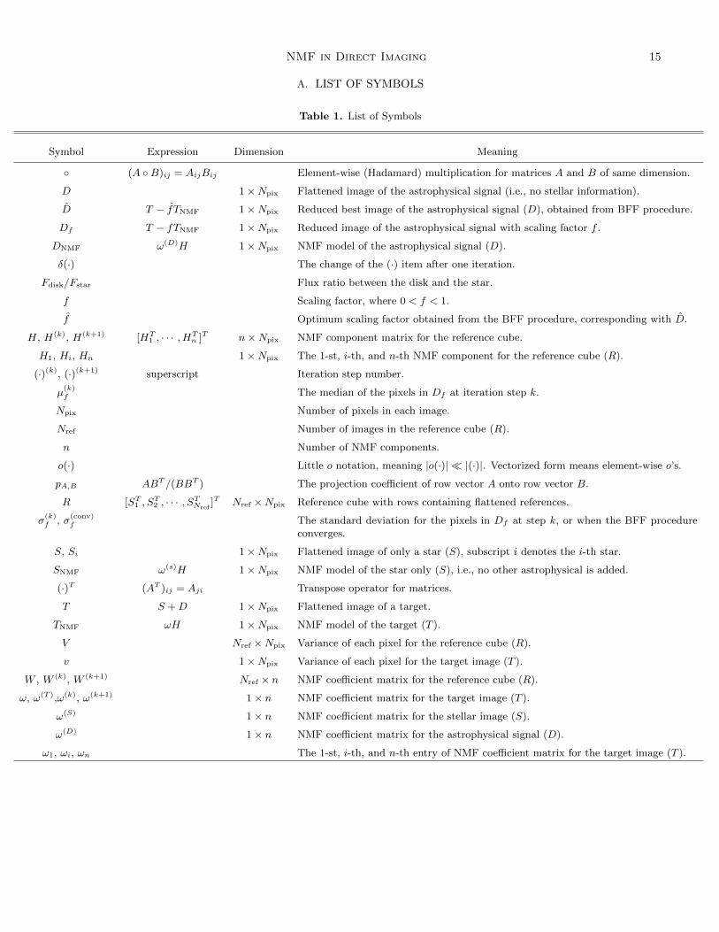
A. LIST OF SYMBOLS

Table 1. List of Symbols

Symbol Expression Dimension Meaning

◦ (A ◦B)ij = AijBij Element-wise (Hadamard) multiplication for matrices A and B of same dimension.

D 1×Npix Flattened image of the astrophysical signal (i.e., no stellar information).

D T − fTNMF 1×Npix Reduced best image of the astrophysical signal (D), obtained from BFF procedure.

Df T − fTNMF 1×Npix Reduced image of the astrophysical signal with scaling factor f .

DNMF ω(D)H 1×Npix NMF model of the astrophysical signal (D).

δ(·) The change of the (·) item after one iteration.

Fdisk/Fstar Flux ratio between the disk and the star.

f Scaling factor, where 0 < f < 1.

f Optimum scaling factor obtained from the BFF procedure, corresponding with D.

H, H(k), H(k+1) [HT1 , · · · , HT

n ]T n×Npix NMF component matrix for the reference cube.

H1, Hi, Hn 1×Npix The 1-st, i-th, and n-th NMF component for the reference cube (R).

(·)(k), (·)(k+1) superscript Iteration step number.

µ(k)f The median of the pixels in Df at iteration step k.

Npix Number of pixels in each image.

Nref Number of images in the reference cube (R).

n Number of NMF components.

o(·) Little o notation, meaning |o(·)| � |(·)|. Vectorized form means element-wise o’s.

pA,B ABT /(BBT ) The projection coefficient of row vector A onto row vector B.

R [ST1 , S

T2 , · · · , ST

Nref]T Nref ×Npix Reference cube with rows containing flattened references.

σ(k)f , σ

(conv)f The standard deviation for the pixels in Df at step k, or when the BFF procedure

converges.

S, Si 1×Npix Flattened image of only a star (S), subscript i denotes the i-th star.

SNMF ω(s)H 1×Npix NMF model of the star only (S), i.e., no other astrophysical is added.

(·)T (AT )ij = Aji Transpose operator for matrices.

T S +D 1×Npix Flattened image of a target.

TNMF ωH 1×Npix NMF model of the target (T ).

V Nref ×Npix Variance of each pixel for the reference cube (R).

v 1×Npix Variance of each pixel for the target image (T ).

W , W (k), W (k+1) Nref × n NMF coefficient matrix for the reference cube (R).

ω, ω(T ),ω(k), ω(k+1) 1× n NMF coefficient matrix for the target image (T ).

ω(S) 1× n NMF coefficient matrix for the stellar image (S).

ω(D) 1× n NMF coefficient matrix for the astrophysical signal (D).

ω1, ωi, ωn The 1-st, i-th, and n-th entry of NMF coefficient matrix for the target image (T ).

16 Ren et al.

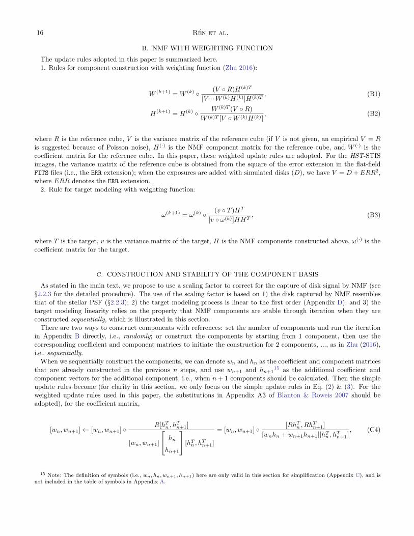
B. NMF WITH WEIGHTING FUNCTION

The update rules adopted in this paper is summarized here.

1. Rules for component construction with weighting function (Zhu 2016):

W (k+1) = W (k) ◦ (V ◦R)H(k)T

[V ◦W (k)H(k)]H(k)T, (B1)

H(k+1) = H(k) ◦ W (k)T (V ◦R)

W (k)T [V ◦W (k)H(k)], (B2)

where R is the reference cube, V is the variance matrix of the reference cube (if V is not given, an empirical V = R

is suggested because of Poisson noise), H(·) is the NMF component matrix for the reference cube, and W (·) is the

coefficient matrix for the reference cube. In this paper, these weighted update rules are adopted. For the HST-STIS

images, the variance matrix of the reference cube is obtained from the square of the error extension in the flat-field

FITS files (i.e., the ERR extension); when the exposures are added with simulated disks (D), we have V = D+ERR2,

where ERR denotes the ERR extension.

2. Rule for target modeling with weighting function:

ω(k+1) = ω(k) ◦ (v ◦ T )HT

[v ◦ ω(k)]HHT, (B3)

where T is the target, v is the variance matrix of the target, H is the NMF components constructed above, ω(·) is the

coefficient matrix for the target.

C. CONSTRUCTION AND STABILITY OF THE COMPONENT BASIS

As stated in the main text, we propose to use a scaling factor to correct for the capture of disk signal by NMF (see

§2.2.3 for the detailed procedure). The use of the scaling factor is based on 1) the disk captured by NMF resembles

that of the stellar PSF (§2.2.3); 2) the target modeling process is linear to the first order (Appendix D); and 3) the

target modeling linearity relies on the property that NMF components are stable through iteration when they are

constructed sequentially, which is illustrated in this section.

There are two ways to construct components with references: set the number of components and run the iteration

in Appendix B directly, i.e., randomly; or construct the components by starting from 1 component, then use the

corresponding coefficient and component matrices to initiate the construction for 2 components, ..., as in Zhu (2016),

i.e., sequentially.

When we sequentially construct the components, we can denote wn and hn as the coefficient and component matrices

that are already constructed in the previous n steps, and use wn+1 and hn+115 as the additional coefficient and

component vectors for the additional component, i.e., when n+ 1 components should be calculated. Then the simple

update rules become (for clarity in this section, we only focus on the simple update rules in Eq. (2) & (3). For the

weighted update rules used in this paper, the substitutions in Appendix A3 of Blanton & Roweis 2007 should be

adopted), for the coefficient matrix,

[wn, wn+1]← [wn, wn+1] ◦R[hTn , h

Tn+1]

[wn, wn+1]

hn

hn+1

[hTn , hTn+1]

= [wn, wn+1] ◦[RhTn , Rh

Tn+1]

[wnhn + wn+1hn+1][hTn , hTn+1]

, (C4)

15 Note: The definition of symbols (i.e., wn, hn, wn+1, hn+1) here are only valid in this section for simplification (Appendix C), and isnot included in the table of symbols in Appendix A.

NMF in Direct Imaging 17

where the left arrow (←) is a simplified notation of the updating procedure, where the left side is the result in the

(k + 1)-th step, and the right side contains the results from the (k)-th step. For the component matrix,

hn

hn+1

← hn

hn+1

◦ wT

n

wTn+1

R wT

n

wTn+1

[wn, wn+1]

hn

hn+1

=

hn

hn+1

◦ wT

nR

wTn+1R

wT

nwn wTnwn+1

wTn+1wn wT

n+1wn+1

hn

hn+1

. (C5)

Focusing on the individual matrices, we have

wn ← wn ◦RhTn

wnhnhTn + wn+1hn+1hTn= wn ◦

RhTnwnhnhTn

◦ 1

1 +wn+1hn+1hT

n

wnhnhTn

, (C6)

hn ← hn ◦wT

nR

wTnwnhn + wT

nwn+1hn+1= hn ◦

wTnR

wTnwnhn

◦ 1

1 +wT

nwn+1hn+1

wTnwnhn

, (C7)

wn+1 ← wn+1 ◦RhTn+1

wnhnhTn+1 + wn+1hn+1hTn+1

= wn+1 ◦RhTn+1

wnhnhTn+1

◦ 1

1 +wn+1hn+1hT

n+1

wnhnhTn+1

, (C8)

hn+1 ← hn+1 ◦wT

n+1R

wTn+1wnhn + wT

n+1wn+1hn+1= hn+1 ◦

wTn+1R

wTn+1wnhn

◦ 1

1 +wT

n+1wn+1hn+1

wTn+1wnhn

. (C9)

Given that

(a) when n = m, the coefficient matrix wn and component matrix hn already satisfy R ≈ wnhn, and

(b) the new coefficient and component vectors (wn+1 and hn+1) are randomly initialized (Zhu 2016): the elements

are drawn from a uniform distribution from 0 to 1,

the change of hn in the first iteration of in Eq. (C7) before (holdn ) and after (hnewn ) the inclusion of wn+1 and hn+1

gives

δhn = hnewn − holdn (C10)

=

1

1 +wT

nwn+1hn+1

wTnwnhn

− 1

◦ hn ◦ wTnR

wTnwnhn

(C11)

=

1

1 +wT

nwn+1hn+1

wTnwnhn

− 1

◦ holdn . (C12)

Lemma (Stability) : For the individual elements (R(·)j) in the reference cube, if the R(·)j ’s are sufficiently large

(for our purpose, they should have large signal-to-noise ratios), then the update has little impact on the constructed

components (i.e., hn) if we construct the components sequentially.

Proof: In high-contrast imaging, if the values of the pixels in the references are large, R(·)j can be represented by

R(·)j � 1, (C13)

which, when accompanied with an weighting function as adopted in our paper (see Appendix B, as well as Blanton &

Roweis 2007), the pixels should have large signal-to-noise ratios, i.e.,

SNR(·)j =R(·)j√V(·)j

� 1. (C14)

To simplify our derivation, the above representation of signal-to-noise ratio is represented by R(·)j in this section. This

simplification is in principle valid following the substitution as in Blanton & Roweis (2007).

18 Ren et al.

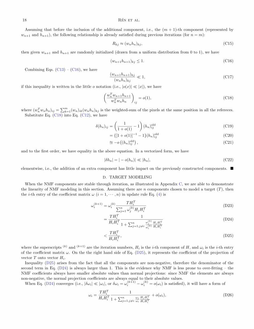
Assuming that before the inclusion of the additional component, i.e., the (m + 1)-th component (represented by

wn+1 and hn+1), the following relationship is already satisfied during previous iterations (for n = m):

Rkj ≈ (wnhn)kj , (C15)

then given wn+1 and hn+1 are randomly initialized (drawn from a uniform distribution from 0 to 1), we have

(wn+1hn+1)kj ≤ 1. (C16)

Combining Eqs. (C13) – (C16), we have(wn+1hn+1)kj

(wnhn)kj� 1, (C17)

if this inequality is written in the little o notation (i.e., |o(x)| � |x|), we have(wT

nwn+1hn+1

wTnwnhn

)ij

= o(1), (C18)

where (wTnwnhn)ij =

∑mk=1(wn)ik(wnhn)kj is the weighted-sum of the pixels at the same position in all the refereces.

Substitute Eq. (C18) into Eq. (C12), we have

δ(hn)ij =

(1

1 + o(1)− 1

)(hn)oldij (C19)

= {[1 + o(1)]−1 − 1}(hn)oldij (C20)

u −o((hn)oldij

), (C21)

and to the first order, we have equality in the above equation. In a vectorized form, we have

|δhn| = | − o(hn)| � |hn|, (C22)

elementwise, i.e., the addition of an extra component has little impact on the previously constructed components. �

D. TARGET MODELING

When the NMF components are stable through iteration, as illustrated in Appendix C, we are able to demonstrate

the linearity of NMF modeling in this section. Assuming there are n components chosen to model a target (T ), then

the i-th entry of the coefficient matrix ω (i = 1, · · · , n) in update rule Eq. (4) is

ω(k+1)i = ω

(k)i

THTi∑n

j=1 ω(k)j HjHT

i

(D23)

=THT

i

HiHTi

1

1 +∑n

j=1,j 6=i

ω(k)j

ω(k)i

HjHTi

HiHTi

(D24)

<THT

i

HiHTi

, (D25)

where the superscripts (k) and (k+1) are the iteration numbers, Hi is the i-th component of H, and ωi is the i-th entry

of the coefficient matrix ω. On the the right hand side of Eq. (D25), it represents the coefficient of the projection of

vector T onto vector Hi.

Inequality (D25) arises from the fact that all the components are non-negative, therefore the denominator of the

second term in Eq. (D24) is always larger than 1. This is the evidence why NMF is less prone to over-fitting – the

NMF coefficients always have smaller absolute values than normal projections: since NMF the elements are always

non-negative, the normal projection coefficients are always equal to their absolute values.

When Eq. (D24) converges (i.e., |δωi| � |ωi|, or δωi = ω(k+1)i − ω(k)

i = o(ωi) is satisfied), it will have a form of

ωi =THT

i

HiHTi

1

1 +∑n

j=1,j 6=iωj

ωi

HjHTi

HiHTi

+ o(ωi), (D26)

NMF in Direct Imaging 19

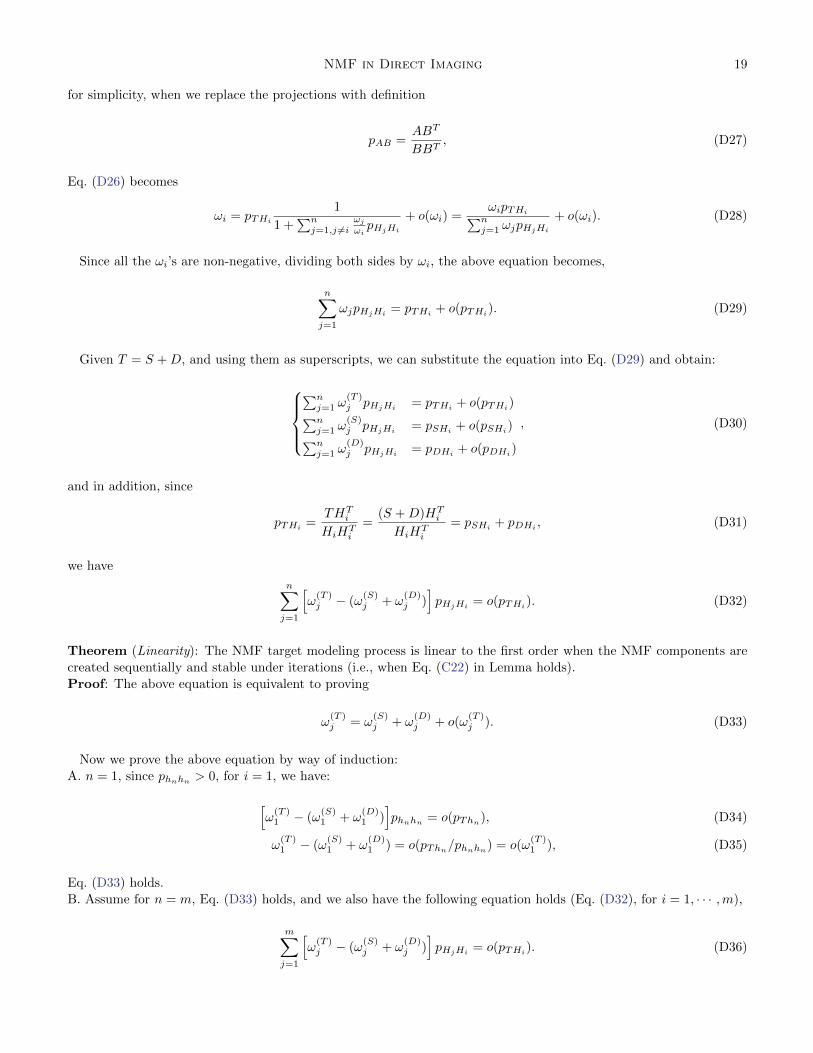
for simplicity, when we replace the projections with definition

pAB =ABT

BBT, (D27)

Eq. (D26) becomes

ωi = pTHi

1

1 +∑n

j=1,j 6=iωj

ωipHjHi

+ o(ωi) =ωipTHi∑n

j=1 ωjpHjHi

+ o(ωi). (D28)

Since all the ωi’s are non-negative, dividing both sides by ωi, the above equation becomes,

n∑j=1

ωjpHjHi= pTHi

+ o(pTHi). (D29)

Given T = S +D, and using them as superscripts, we can substitute the equation into Eq. (D29) and obtain:

∑n

j=1 ω(T )j pHjHi = pTHi + o(pTHi)∑n

j=1 ω(S)j pHjHi = pSHi + o(pSHi)∑n

j=1 ω(D)j pHjHi = pDHi + o(pDHi)

, (D30)

and in addition, since

pTHi=

THTi

HiHTi

=(S +D)HT

i

HiHTi

= pSHi + pDHi , (D31)

we have

n∑j=1

[ω(T )j − (ω

(S)j + ω

(D)j )

]pHjHi

= o(pTHi). (D32)

Theorem (Linearity): The NMF target modeling process is linear to the first order when the NMF components are

created sequentially and stable under iterations (i.e., when Eq. (C22) in Lemma holds).Proof: The above equation is equivalent to proving

ω(T )j = ω

(S)j + ω

(D)j + o(ω

(T )j ). (D33)

Now we prove the above equation by way of induction:

A. n = 1, since phnhn> 0, for i = 1, we have:

[ω(T )1 − (ω

(S)1 + ω

(D)1 )

]phnhn

= o(pThn), (D34)

ω(T )1 − (ω

(S)1 + ω

(D)1 ) = o(pThn/phnhn) = o(ω

(T )1 ), (D35)

Eq. (D33) holds.

B. Assume for n = m, Eq. (D33) holds, and we also have the following equation holds (Eq. (D32), for i = 1, · · · ,m),

m∑j=1

[ω(T )j − (ω

(S)j + ω

(D)j )

]pHjHi

= o(pTHi). (D36)

20 Ren et al.

C. For n = m+ 1, given the fact that the components do not vary to the first order when the number of components

increases (Appendix C Conclusion), for i = 1, · · · ,m, Eq. (D32) becomes,

o(pTHi) =

m+1∑j=1

{ω(T )j − [ω

(S)j + ω

(D)j ]

}p[Hj+o(Hj)][(Hi+o(Hi)]

=

m∑j=1

{ω(T )j − [ω

(S)j + ω

(D)j ]

}[pHjHi

+ 2o(pHjHi) + o2(pHjHi

)]

+{ω(T )m+1 − [ω

(S)m+1 + ω

(D)m+1]

}[pHm+1Hi

+ o(pHm+1Hi)]

=o(pTHi) +

m∑j=1

{ω(T )j − [ω

(S)j + ω

(D)j ]

}[2o(pHjHi

) + o2(pHjHi)]

+{ω(T )m+1 − [ω

(S)m+1 + ω

(D)m+1]

}[pHm+1Hi

+ o(pHm+1Hi)]

where Eq. (D36) is substituted into Eq. (D32) in the above derivation. Since pHm+1Hi is a simple number rather than

a vector, and Eq. (D33) holds, by keeping up to the first order, we have

ω(T )m+1 − [ω

(S)m+1 + ω

(D)m+1] =

o(pTHi)−

∑mj=1

{ω(T )j − [ω

(S)j + ω

(D)j ]

}[2o(pHjHi

) + o2(pHjHi)]

pHm+1Hi + o(pHm+1Hi)(D37)

=o(pTHi

)− 2o2(pTHi)− o3(pTHi

)

pHm+1Hi+ o(pHm+1Hi

)=

o(pTHi)

pHm+1Hi

(D38)

= o(ω(T )m+1), (D39)

which is also true when i = m+ 1, therefore the proof of Eq. (D33) is complete.

Rewrite Eq. (D33) in vector form, we have

ω(T ) = ω(S) + ω(D) + o(ω(T )), (D40)

and thus

TNMF = ω(T )H = ω(S)H + ω(D)H + o(ω(T )H) (D41)

= SNMF +DNMF + o(TNMF), (D42)

i.e., to the first order, we can linearly separate the stellar PSF and speckles from the circumstellar disk signal. �

E. THE BEST FACTOR FINDING (BFF) PROCEDURE

We notice that when the optimum scaling factor is in effect (§2.2.3), the diskless regions should be well modeled by

the NMF model of the target and therefore the values on these pixels should be small and have a histogram distribution

that is symmetric about 0. Consequently, the variation of the noise of the diskless region should be minimized. We

thus introduce the BFF procedure as follows to find this factor:

1. For each target (T ), construct its NMF model (TNMF) with the component basis (H), then vary the scaling factor

(f) from 0 to 1, creating several scaled reduced images (Df = T − fTNMF).

2. For each scaled reduced image (Df ),

(a) Identification of the background region iteratively: in each iteration (k), find the median (µ(k)f ) and standard

deviation (σ(k)f ) of Df , remove the pixels with values satisfying the condition:

value > µ(k)f + 3σ

(k)f or value < µ

(k)f − 10σ

(k)f .

These pixels are treated as non-background ones because of their large deviations from the median. Repeat this process

until the number of background pixels does not change.

(b) Calculation of the noise in the diskless region: calculate the standard deviation of the remaining pixels when

step (a) converges, and denote it by σ(conv)f .

NMF in Direct Imaging 21

3. The factor corresponding with the minimum standard deviation of Df of the diskless pixels will be taken as the

best one (f), i.e.,

f = arg minf

σ(conv)f .

The connection between BFF and the classical optimum scaling factor is that both of them are minimizing the

residual noise. In comparison, the classical method minimizes the residual noise along the major diffraction spikes

after PSF subtraction (e.g., Schneider et al. 2009). When the diffraction spikes are not stable, especially for ground-

based observations, BFF is able to focus on the entire field of view, and is more able to minimize the overall difference

between the PSF template and the target.

REFERENCES

Amara, A., & Quanz, S. P. 2012, MNRAS, 427, 948

Biller, B. A., Close, L., Lenzen, R., et al. 2004, in

Proc. SPIE, Vol. 5490, Advancements in Adaptive

Optics, ed. D. Bonaccini Calia, B. L. Ellerbroek, &

R. Ragazzoni, 389

Blanton, M. R., & Roweis, S. 2007, AJ, 133, 734

Chen, C. H., Mittal, T., Kuchner, M., et al. 2014, ApJS,

211, 25

Choquet, E., Pueyo, L., Hagan, J. B., et al. 2014, in

Proc. SPIE, Vol. 9143, Space Telescopes and

Instrumentation 2014: Optical, Infrared, and Millimeter

Wave, 914357

Choquet, E., Perrin, M. D., Chen, C. H., et al. 2016, ApJL,

817, L2

Choquet, E., Milli, J., Wahhaj, Z., et al. 2017, ApJL, 834,

L12

Debes, J. H., Jang-Condell, H., Weinberger, A. J., Roberge,

A., & Schneider, G. 2013, ApJ, 771, 45

Debes, J. H., Poteet, C. A., Jang-Condell, H., et al. 2017,

ApJ, 835, 205

Dong, R., & Fung, J. 2017, ApJ, 835, 146

Dong, R., Zhu, Z., Fung, J., et al. 2016, ApJL, 816, L12

Dong, R., Zhu, Z., Rafikov, R. R., & Stone, J. M. 2015a,

ApJL, 809, L5

Dong, R., Zhu, Z., & Whitney, B. 2015b, ApJ, 809, 93

Esposito, T. M., Fitzgerald, M. P., Graham, J. R., & Kalas,

P. 2014, ApJ, 780, 25

Follette, K. B., Rameau, J., Dong, R., et al. 2017, AJ, 153,

264

Gomez Gonzalez, C. A., Wertz, O., Absil, O., et al. 2017,

AJ, 154, 7

Grady, C. A., Hamaguchi, K., Schneider, G., et al. 2010,

ApJ, 719, 1565

Grady, C. A., Muto, T., Hashimoto, J., et al. 2013, ApJ,

762, 48

Hinkley, S., Oppenheimer, B. R., Soummer, R., et al. 2007,

ApJ, 654, 633

Jang-Condell, H., & Boss, A. P. 2007, ApJL, 659, L169

Jang-Condell, H., & Turner, N. J. 2012, ApJ, 749, 153

—. 2013, ApJ, 772, 34

Krist, J. E., Hook, R. N., & Stoehr, F. 2011, in Proc. SPIE,

Vol. 8127, Optical Modeling and Performance Predictions

V, 81270J

Lafreniere, D., Marois, C., Doyon, R., & Barman, T. 2009,

ApJL, 694, L148

Lafreniere, D., Marois, C., Doyon, R., Nadeau, D., &

Artigau, E. 2007, ApJ, 660, 770

Lee, D. D., & Seung, H. S. 2001, in Advances in Neural

Information Processing Systems 13, ed. T. K. Leen, T. G.

Dietterich, & V. Tresp (MIT Press), 556

Lee, E. J., & Chiang, E. 2016, ApJ, 827, 125

Marino, S., Matra, L., Stark, C., et al. 2016, MNRAS, 460,

2933

Marois, C., Lafreniere, D., Doyon, R., Macintosh, B., &

Nadeau, D. 2006, ApJ, 641, 556

Marois, C., Macintosh, B., & Veran, J.-P. 2010, in

Proc. SPIE, Vol. 7736, Adaptive Optics Systems II,

77361J

Mawet, D., Pueyo, L., Lawson, P., et al. 2012, in

Proc. SPIE, Vol. 8442, Space Telescopes and

Instrumentation 2012: Optical, Infrared, and Millimeter

Wave, 844204

Mazoyer, J., Boccaletti, A., Augereau, J.-C., et al. 2014,

A&A, 569, A29

Mazoyer, J., Boccaletti, A., Choquet, E., et al. 2016, ApJ,

818, 150

Milli, J., Lagrange, A.-M., Mawet, D., et al. 2014, A&A,

566, A91

Nesvold, E. R., Naoz, S., Vican, L., & Farr, W. M. 2016,

ApJ, 826, 19

Paatero, P., & Tapper, U. 1994, Environmetrics, 5, 111

Perrin, M. D., Graham, J. R., Kalas, P., et al. 2004,

Science, 303, 1345

Perrin, M. D., Graham, J. R., & Lloyd, J. P. 2008, PASP,

120, 555

22 Ren et al.

Pinte, C., Harries, T. J., Min, M., et al. 2009, A&A, 498,

967

Pinte, C., Menard, F., Duchene, G., & Bastien, P. 2006,

A&A, 459, 797

Pueyo, L. 2016, ApJ, 824, 117

Pueyo, L., Crepp, J. R., Vasisht, G., et al. 2012, ApJS, 199,

6

Pueyo, L., Soummer, R., Hoffmann, J., et al. 2015, ApJ,

803, 31

Ren, B., Pueyo, L., Perrin, M. D., Debes, J. H., & Choquet,

E. 2017, in Proc. SPIE, Vol. 10400, Techniques and

Instrumentation for Detection of Exoplanets VIII,

1040021

Riley, A. 2017, STIS Instrument Hanbook for Cycle 25,

Version 16.0

Rodigas, T. J., Malhotra, R., & Hinz, P. M. 2014, ApJ,

780, 65

Schneider, G., Weinberger, A. J., Becklin, E. E., Debes,

J. H., & Smith, B. A. 2009, AJ, 137, 53

Schneider, G., Grady, C. A., Hines, D. C., et al. 2014, AJ,

148, 59

Schneider, G., Grady, C. A., Stark, C. C., et al. 2016, AJ,

152, 64

Smith, B. A., & Terrile, R. J. 1984, Science, 226, 1421

Soummer, R., Ferrari, A., Aime, C., & Jolissaint, L. 2007,

ApJ, 669, 642

Soummer, R., Pueyo, L., & Larkin, J. 2012, ApJL, 755, L28

Soummer, R., Perrin, M. D., Pueyo, L., et al. 2014, ApJL,

786, L23

Stark, C. C., Schneider, G., Weinberger, A. J., et al. 2014,

ApJ, 789, 58

Traub, W. A., & Oppenheimer, B. R. 2010, Direct Imaging

of Exoplanets, ed. S. Seager, 111

Wahhaj, Z., Cieza, L. A., Mawet, D., et al. 2015, A&A,

581, A24

Wang, J. J., Ruffio, J.-B., De Rosa, R. J., et al. 2015,

pyKLIP: PSF Subtraction for Exoplanets and Disks,

Astrophysics Source Code Library, ascl:1506.001

Zhu, G. 2016, ArXiv e-prints, arXiv:1612.06037 [astro-ph.IM]

Zhu, Z., Dong, R., Stone, J. M., & Rafikov, R. R. 2015,

ApJ, 813, 88