TWO-DIMENSIONAL NON NEWTONIAN FLUID INJECTION MOULDING

FILLING IMPROVED WITH A CVFEM/VOF METHOD

C.H. Salinas1, D.A. Vasco

2, N.O. Moraga

3

1 Department of Mechanical Engineering, University of Bío-Bío (casali@ubiobio.cl)

2Department of Mechanical Engineering, University of Santiago de Chile

3Department of Mechanical Engineering, University of La Serena

Abstract. A new method based on volume of fluid (VOF) for interface tracking in the simula-

tion of injection molding is presented. The proposed method is comprised by two main stages:

accumulation and distribution of the volume fraction. In the first stage the equation for the

volume fraction with a non-interfacial flux condition is solved meanwhile in the second stage

the accumulated volume of fluid that arises as a consequence of the application of the first

one is dispersed. This procedure guarantees that the fluid fills the available space without

dispersion of the interface. The mathematical model is based on two-phase transport equa-

tions which are numerically integrated through the Control Volume Finite Element Method

(CVFEM). The numerical results for the interface position are validated with experimental

results and numerical data available in the literature. The transient position of the advance

fronts showed an effective and consistent simulation of an injection molding process. The

non-dispersive VOF method here proposed will be implemented for the simulation of non-

isothermal injection molding in two-dimensional cavities.

Keywords: Free surface, Eulerian, Finite volume, Navier-Stokes, Laminar flow.

1. INTRODUCTION

Several studies have been focused on the development of efficient methods and algo-

rithms for the accurate prediction of the position of an interface in biphasic fluid flow. Alt-

hough the applications may be numerous, the reported results mainly deal with industrial pro-

cesses such as polymer injection molding [9, 14, 7] and metal casting [6, 12, 13].

The methods employed for interface tracking are classified according to the domain

discretization. In the variable grid methods, known as well as Lagrangian methods, the inter-

face coincides with the front of the moving grid, which has to be redefined after each time

step [3, 10]. For the fixed grid or Eulerian methods [11, 21], the grid is unique and remains

constant during the whole calculation process.

The volume of fluid (VOF) method proposed by Hirt and Nichols [8] is a commonly

used fixed grid technique mainly due to the simplicity of its formulation. Broadly speaking,

Blucher Mechanical Engineering ProceedingsMay 2014, vol. 1 , num. 1www.proceedings.blucher.com.br/evento/10wccm

the VOF formulation is a conservation equation which describes the convective transport of

the volume of fluid fraction or simply the volume fraction. The numerical solution of the VOF

differential equation leads to the numerical dispersion of the interface, normally known as

numerical smearing.

Several pioneering works have implemented alternatives in order to avoid the disper-

sion of the interface. Estacio and Mangiavacchi [5] proposed an approach for the numerical

solution of the VOF convective equation that restricts the fluid flow only from the completely

filled control volumes. The effect of numerical smearing of the interface is diminished by

calculation of a variable time step which assures that the control volumes next to the interface

will be completely filled.

Kim and Lee [10] implemented an explicit formulation of the VOF equation on terms

of the actual fractional volume of fluid which is a measure of the wetted area of the boundary

of a control volume. In this method, the effective volume of a cell is calculated as a function

of the orientation vector of the free surface and the value of the volume fraction in such a cell.

On the other hand, the fluid flow through the boundary of a cell is calculated as a function of

the fractional volume of fluid instead of the volume fraction.

Cruchaga et al. [3] proposed that the discontinuous function which represents the in-

terface position could be approximated through a continuous derivable function. Neverthe-

less, in their work the authors emphasized that the discontinuous function which represents

the position of the interface should be recovered from the continuous function by means of

minimum squares projection. The calculation of the mixture properties, for instance is made

by using the discontinuous function.

A modification of the VOF equation was proposed by Swaminathan and Voller [19]

through the implementation of a variable (G) instead of the volume fraction (F) in the convec-

tive term. The transport properties for each phase are calculated according to the F and G val-

ues obtained in the domain in such a way that the flow of the liquid phase takes place only

from the completely filled control volumes.

The control volume finite element method (CVFEM) was developed by Baliga and

Patankar [1]. This method may be considered as a hybrid method made up from combining

the finite-element method (FEM) and finite-volume method (FVM). CVFEM possess the var-

iational analysis advantages of FEM and the conservativeness properties of FVM.

In the present work the CVFEM method is used for the numerical integration of the

coupled continuity, Navier-Stokes equations, with a new model based on VOF, for the simu-

lation of the filling process in two-dimensional cavities. The dispersion of the interface is nul-

lified through the implementation of a new scheme, performed in two main stages denominat-

ed accumulation and distribution. In the first stage, the VOF equation with a non-interfacial

flux condition is numerically solved, meanwhile in the second stage the accumulated volume

of fluid is dispersed. The implementation of this method is conditioned to a non-smear dis-

placement of the interface. The CVFEM method is implemented with an Euler implicit for-

mulation to advance in time while central differences and an exponential interpolation scheme

for the diffusive and convective terms, respectively. The implemented method is verified

through reported experimental [18] and numerical data [3].

2. MATHEMATICAL AND NUMERICAL MODELING

The mathematical model consists of a set of second order non-linear partial differential

equations which represents mass conservation (1), Navier-Stokes and volume fraction (3).

This set of equations, settled for a two-dimensional two-phase space xi (i=1, 2) describes the

transient behavior of the pressure, and the volume fraction (F). An incompressible Newtonian

fluid of viscosity (µ) and constant density () is considered.

. (1)

(2)

. (3)

The mathematical model expressed by Equations (1)-(3) can be represented by a gen-

eral convective-diffusive transport Equation (4).

. (4)

The integration of Equation (4) in a two-dimensional space of volume V discretized by

finite volumes (FV) of volume Vn

and surface Sn, with n=1...N, using the Green’s Theorem

gives:

(5)

where each FV of volume Vn consists of the partial contributions Ve (e=1,..,E) of FE

(Figure 1), according to:

(6)

and the segments Sn are defined as

(7a)

Each segment is comprised by two line segments. The FV is centered in the local

vertex 1:

(7b)

with the vectors (na, nb) normal to the line segments drawn from side midpoints (a, c)

to the centroid (G) of the FE, as it is shown in Figure 2.

Figure 1. Discretized representation of a two-dimensional domain by CVFEM.

Figure 2. Local system of coordinates (Y, Z) represented on a finite element.

Integration of the convective and diffusive terms of Equation (5) requires a function

that represents the variation of the variable in each FE. A linear function (8a) is adopted for

the diffusive term in order to represent the -variation meanwhile an exponential function

(8b) is adopted for the convective term:

(8a)

(8b)

where the coefficients A, B and C are defined as a function of the nodal values of the

dependent variable and the coordinates of the vertices of the FE. The interpolated -value

in Equation (8a) is evaluated as a function of the global coordinate values (x, y).

For the linear interpolation of the Equation (8b), the coordinates of the vertices of each

FE are defined according to a local system of coordinates (Z, Y), where the Z-axis is parallel

to the vector velocity Vi with module U (Figure 2). Z is expressed as an exponential function

of the global coordinate x and the Peclet number (9):

3

2 a

Finite volumen FV

Finite element FE

a, b and c midpoints (sides of the FE)

G 1,2,3 Local numering of the vertices b

c

1

bn cn

an

3

2 1

c

a

b

G

an

bn cn Z

Y U

(9)

An implicit Euler scheme, added to the previous description for the spatial integration,

is used in order to integrate the transient term of Equation (4). In this way a linear system of

algebraic equations is generated and then solved through the SOR Gauss-Seidel iterative

method. More details about the computational implementation can be found in the work of

Salinas et al. [17].

3. PROPOSED VOF MODEL

In this section the proposed VOF model is described. First, a variable (G) is introduced

in the convective term of the VOF equation. This variable gathers the discontinuous nature of

the function that describes the position of the interface. The implemented G-variable has

mainly a restrictive role of the fluid flow through the boundaries of the FV´s adjacent to the

interface. Unlike the method of Swaminathan and Voller [19], an advantage of the implemen-

tation of this new variable in the VOF equation is that an iterative process for the determina-

tion of the interface position is not required.

The calculation of the volume fraction and therefore the position of the interface are

obtained through the implementation of two main stages denominated accumulation and dis-

tribution. In the first stage, the VOF equation with a non-interfacial flux condition is solved.

As a consequence, for a set of FV the condition that F>1 will be obtained. In the second stage

the accumulated volume of fluid is dispersed between the adjacent FV´s with F<1. The intrin-

sic discontinuous nature of the function that describes the position of the interface is met by

the distribution stage; therefore the numerical smearing of the interface is avoided. Both stag-

es will be better described through their implementation in the following formulations.

2.1. One-dimensional Formulation

An initially empty duct of length L and constant transversal section is considered. The

duct is being filled with a fluid that enters at a constant velocity U in x=0 (Figure 3). In this

formulation, the VOF equation is modified with the parameter (G) as:

(10)

The convective term of the Equation (10) is integrated according to CVFEM for the

domain of length L discretized by FV (Vn with n=1…N) introducing the upwind interpolation.

Meanwhile the transient term is integrated through an explicit Euler scheme. In this way, for a

FV centered on P the following equation is obtained:

(11)

where Cr is the non-dimensional Courant number and the subscript W refers to the G-value of

the FV centered on a node at the right of the FV centered on P.

Figure 3. Filling process scheme for one-dimensional duct.

The following three steps procedure allows the solution of the filling process for the

described one-dimensional duct from the initial time t=t0

to t=t0+dt. Initially, the values of F

and G are considered null in the entire domain but in the inlet position where F=G=1.

Step 1: Calculation of the present value of F according to:

(12)

where the values of G are obtained through:

(13)

This step is considered the accumulation stage since it will be found that there is a FV

with F>1.

Step 2: Calculation of the correction factor of the Courant number ( ) according to the

corresponding F-value:

(14)

This factor modifies Cr allowing for the distribution of the excess volume of fluid to

the adjacent FV located at the right. The Courant number is now defined as:

oCr Cr (15)

The calculations (12) and (14) are performed for each FV of volume Vn with n=1,…,N.

Step 3: In the last step, previously to the next time step, the values of F are updated

according to:

FW=1 0<FP<1 FE=0

U

G=1; F=1 X

1 2 3 p P+1 P-1

(16a)

(16b)

Through the implementation of the described algorithm for a duct of unit length and

Cr=1.2, the results for the volume fraction shown in the Table 1 are calculated. These results

are exactly the same as those obtained by Swaminathan and Voller [19], by using an iterative

algorithm. It is evident that the proposed method avoids the dispersion of the interface noticed

when the classic VOF method is implemented.

Table 2. Transient results of the volume fraction for the filling process of the unit length one-

dimensional duct with Cr = 1.2 described in Figure 3.

node/t 0.12 0.24 0.36 0.48

0 1.0 1.0 1.0 1.0

1 1.0 1.0 1.0 1.0

2 0.2 1.0 1.0 1.0

3 0.0 0.4 1.0 1.0

4 0.0 0.0 0.6 1.0

5 0.0 0.0 0.0 0.8

2.2. Two-dimensional formulation

Here, a 2D discretized domain according to the formulation of the CVFEM method is

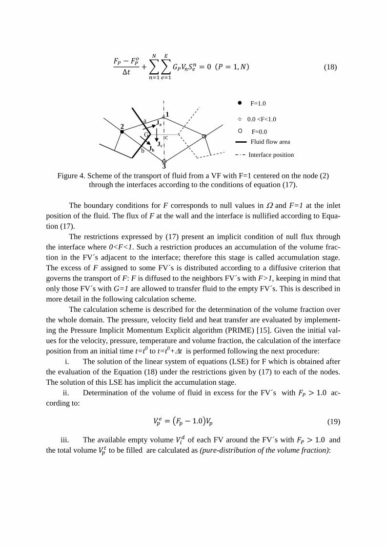
treated. In Figure 4 a part of a FV conformed by a FE which represents the three possible F-

values is shown. Let , and be the fluxes of F through the line segments drawn from the

midpoints of the sides of the FE (a, b and c) to the centroid G. The condition that only the

fluid flows from filled FV is accomplished by the implementation of the conditions in Equa-

tion (17). According to this condition, in the Figure 4 only and would be non-null fluxes

of F

(17)

with G=0 if F<1 or G=1 if F1.

The discretized form of Equation 4 modified with the parameter G, considering an im-

plicit Euler scheme to calculate the transient term and the upwind scheme for the evaluation

of the fluxes of the fraction of volume, is given by:

(18)

Figure 4. Scheme of the transport of fluid from a VF with F=1 centered on the node (2)

through the interfaces according to the conditions of equation (17).

The boundary conditions for F corresponds to null values in and F=1 at the inlet

position of the fluid. The flux of F at the wall and the interface is nullified according to Equa-

tion (17).

The restrictions expressed by (17) present an implicit condition of null flux through

the interface where 0<F<1. Such a restriction produces an accumulation of the volume frac-

tion in the FV´s adjacent to the interface; therefore this stage is called accumulation stage.

The excess of F assigned to some FV´s is distributed according to a diffusive criterion that

governs the transport of F: F is diffused to the neighbors FV´s with F>1, keeping in mind that

only those FV´s with G=1 are allowed to transfer fluid to the empty FV´s. This is described in

more detail in the following calculation scheme.

The calculation scheme is described for the determination of the volume fraction over

the whole domain. The pressure, velocity field and heat transfer are evaluated by implement-

ing the Pressure Implicit Momentum Explicit algorithm (PRIME) [15]. Given the initial val-

ues for the velocity, pressure, temperature and volume fraction, the calculation of the interface

position from an initial time t=t0 to t=t

0+t is performed following the next procedure:

i. The solution of the linear system of equations (LSE) for F which is obtained after

the evaluation of the Equation (18) under the restrictions given by (17) to each of the nodes.

The solution of this LSE has implicit the accumulation stage.

ii. Determination of the volume of fluid in excess for the FV´s with ac-

cording to:

(19)

iii. The available empty volume of each FV around the FV´s with and

the total volume to be filled are calculated as (pure-distribution of the volume fraction):

Jb

F=1.0

0.0 <F<1.0

F=0.0

Fluid flow area

Interface position

c

2

1

3

Ja

b

a

Jc

G

(20)

or according to the fluxes calculated at the interface (flux-based distribution of the volume

fraction). For instance for F2 > 1.0 (see Figure 4), Ja ( ) and Jb (

) are calculated as:

(21)

meanwhile the total flux from the nodes with FP > 1.0 is calculated as the summa-

tion of the nodal fluxes.

iv. The distribution of could be carried out proportionately to the available empty

volume of each neighbor FV i (pure-distribution of the volume fraction approach):

(22)

or through the flux-based distribution approach:

(23)

v. The steps (ii) to (iv) are repeated in such a way that the condition will be

fulfilled for all nodes.

vi. A macroscopic correction of the mass conservation is made in order to avoid nu-

merical errors that could arise because of the raised algorithm. This step is equivalent to the

determination of the macroscopic divergence of F (DF) and its distribution between FV´s ad-

jacent to the interface in a similar way to the performed in the step iv:

0ˆF

S V

D F F F dV n ds (24)

vii. Updating the G values according to:

(25)

2.3. Fluid injection in a rectangular duct

The proposed algorithm for the calculation of the position of the interface is performed

in the injection of an isothermal Newtonian fluid at constant velocity ( ), to a

duct of constant transversal section (0.03m). The dimensions of the duct allow that the wall

effects in the z-direction could be assumed to be negligible, for this reason a two-dimensional

model is appropriate.

Frictionless conditions at the walls are considered as well as fully developed flow at

the outlet. The physical properties of the inlet fluid:

and the air:

are considered constant. In the region where F=0 the pressure is considered null, which is

equivalent to a null traction boundary condition at the interface. The physical properties at

the interface are calculated using the mixture rule using the F-values.

According to the conditions of the problem, the macroscopic mass balance requires

that for each time step Δt the interface moves a length Δx such that Δt=Δx, the same proof was

done by Usnami et al. [20]. The transient position of the interface according to the F and G

values is shown in Figure 5. It can be noticed how the dispersion of the interface is practically

nullified, therefore the interface is located in a narrow region where 0<F<1.

Figure 5. Transient (t=0.05, 0.1 and 0.15s) interface location for the problem of a fluid that

enters at constant velocity to a duct of rectangular constant region (G, continue lines; F

dashed lines).

3. VERIFICATION: FILLING OF A STEP CAVITY

In order to verify the proposed scheme and the implemented numerical code, the fill-

ing process proposed by Dhatt et al. [4] is replicated. In this process, a fluid subjected to grav-

ity enters to a step cavity with a constant velocity (0.1 m/s). Initially the front of the filling

fluid (fluid 1) is located at x=0.02m and the rest of the cavity is occupied by the displaced

fluid (fluid 2). Both fluids are considered Newtonian with constant physical properties. The

F=G=0 F=G=1 F=G=1 G=0

F=0 F=G=1 F=G=0

physical properties of the fluids as well as details of the physical domain are depicted in Fig-

ure 6a.

Free slip condition at the walls of the cavity and fully developed flow at the outlet are

considered as boundary conditions for the velocities. Meanwhile a null traction condition at

the interface is the adopted boundary condition for the pressure.

The discretization of the domain was performed through the implementation of an

open code program EASYMESH, which generates unstructured two-dimensional meshes

based on Delaunay triangulation [2]. A uniform mesh of 1566 nodes shown in Figure 6b is

generated in order to verify the present numerical results and a time step of 0.01s was used in

the calculations.

This physical situation was chosen as well in order to evaluate the ETILT algorithm

developed by Cruchaga et al. [3]. In their work, the finite element method was implemented

and the domain was discretized by an uniform mesh composed of 700 isoparametric four-

noded elements and the use of the time step of 0.01s was reported. The Navier-Stokes equa-

tions were solved through a generalized streamline operator technique.

Figure 6. Physical domain (a) for the filling process of a two-dimensional step cavity and (b)

the mesh used with 1566 nodes and 2888 elements.

The predicted transient position of the interface is in good agreement with those re-

ported in the literature (Figure 7). In this study both approaches previously described for vol-

ume fraction distribution were implemented. Noticeable differences between results are not

observed; in both cases the predicted particular characteristics of the interface are preserved.

Despite of being a filling process influenced by gravity, the way in which the distribution

stage is performed does not affect the shape of the interface, therefore the position of the in-

terface is mainly dependent on the a priori way that the velocity field is calculated.

1 = 100 3 1 = 0.2 2 = 0.1 3 2 = 0.02

0.08m 0.06m

0.03m

0.03m g=10m/s

2

1 2 x

y

a

b

4. VALIDATION: INJECTION MOLDING OF A NEWTONIAN FLUID IN A 2D

CAVITY

In order to validate the proposed scheme and the implemented numerical code, the ex-

perimental filling process studied by Subbiah et al. [18] is replicated. In this experiment, corn

syrup enters to a cavity (0.303m x 0.20 m) with a constant velocity (0.031 m/s) through an

opening (0.02 m), in the upper left side. Both fluids are considered Newtonian, with the same

physical properties used in the duct example. A non-slippery condition at the walls of the cav-

ity and fully developed flow at the outlet are considered as boundary conditions for the ve-

locities. Meanwhile a null traction condition at the interface is the adopted boundary condition

for the pressure.

The mesh study was based on the predicted position of the interface and its difference

respect to the experimental interface position (Figure 8a). The results shows that a better ap-

proximation to the real interface position is achieved with the finer non uniform mesh (5056

nodes, 2661 elements), as it is shown in figure 8b.

t (s) Pure Distribution of F Fluxed-based distribution of F Cruchaga et al.

0.2

0.4

0.8

1.6

2.0

Figure 7. Transient front positions during the filling process of a two-dimensional step cavity

with a Newtonian fluid. Obtained front positions in the present study (columns 1 and 2) and

reference front positions [19] (column 3).

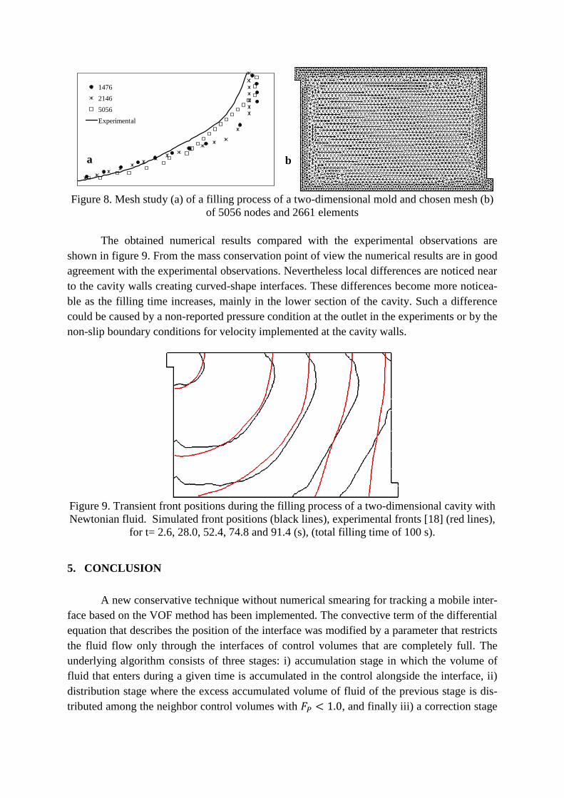
Figure 8. Mesh study (a) of a filling process of a two-dimensional mold and chosen mesh (b)

of 5056 nodes and 2661 elements

The obtained numerical results compared with the experimental observations are

shown in figure 9. From the mass conservation point of view the numerical results are in good

agreement with the experimental observations. Nevertheless local differences are noticed near

to the cavity walls creating curved-shape interfaces. These differences become more noticea-

ble as the filling time increases, mainly in the lower section of the cavity. Such a difference

could be caused by a non-reported pressure condition at the outlet in the experiments or by the

non-slip boundary conditions for velocity implemented at the cavity walls.

Figure 9. Transient front positions during the filling process of a two-dimensional cavity with

Newtonian fluid. Simulated front positions (black lines), experimental fronts [18] (red lines),

for t= 2.6, 28.0, 52.4, 74.8 and 91.4 (s), (total filling time of 100 s).

5. CONCLUSION

A new conservative technique without numerical smearing for tracking a mobile inter-

face based on the VOF method has been implemented. The convective term of the differential

equation that describes the position of the interface was modified by a parameter that restricts

the fluid flow only through the interfaces of control volumes that are completely full. The

underlying algorithm consists of three stages: i) accumulation stage in which the volume of

fluid that enters during a given time is accumulated in the control alongside the interface, ii)

distribution stage where the excess accumulated volume of fluid of the previous stage is dis-

tributed among the neighbor control volumes with , and finally iii) a correction stage

1476

2146

5056

Experimental

a b

during which the excess of volume of fluid occasionally confined in a finite volume is re-

distributed in the interface and an overall correction mass balance is performed.

The numerical code and the implemented scheme has been verified and validated with

available numerical and experimental data for the interface position during mould filling in

one-dimensional and two-dimensional cavities.

Acknowledgements

The authors acknowledge CONICYT-Chile for support received in the FONDECYT

project 1111067. Diego A. Vasco acknowledges the financial support given by the Doctoral

Fellowship of the Advanced Human Capital Program CONICYT-Chile.

6. REFERENCES

[1] Baliga B.R., Patankar S.V., “A new finite element formulation for convection diffusion

problems”. Numer. Heat Transfer, Part B. 3, 393-409, 1980.

[2] Cavendish J.C., Field D.A., Frey W.H., “An Approach to Automatic Three-Dimensional

Finite Element Mesh Generation”. Int. J. Numer. Methods Eng. 21, 329-347, 1985.

[3] Cruchaga M., Celentano D., Tezduyar T.E., “Moving-interface computations with the

edge-tracked interface locator technique (ETILT)”. Int. J. Numer. Methods Fluids. 47,

451–469, 2005.

[4] Dhatt G., Gao D.M., Cheick A.B., “A Finite element simulation of metal flow in moulds”.

Int. J. Numer. Methods Eng. 30, 821-831, 1990.

[5] Estacio K.C., Mangiavacchi N., “Simplified model for mould filling using CVFEM and

unstructured meshes”. Commun. Numer. Methods Eng. 23, 345-361, 2007.

[6] Gao D.M., “A three-dimensional hybrid finite element-volume tracking model for mould

filling in casting processes”. Int. J. Numer. Methods Fluids. 29, 877-895, 1999.

[7] Hieber C.A., Shen S.F., “A finite element/finite difference simulation of the injection

molding filling process”. J. Non-Newtonian Fluid Mech. 7, 1-32, 1980.

[8] Hirt C.W., Nichols B.D., “Volume of Fluid (VOF) method for the dynamics of free

boundaries”. J. Comput. Phys. 39, 201-225, 1981.

[9] Khor C.Y., Ariff Z.M., Ani F.C., Mujeebu M.A., Abdullah M.K., Abdullah M.Z., Joseph

M.A., “Three-dimensional numerical and experimental investigations on polymer rheolo-

gy in meso-scale injection molding”. Int. Commun. Heat Mass Transfer. 37, 131-139,

2010.

[10] Kim M.S., Lee W.I., “A new VOF-based numerical scheme for the simulation of fluid

flow with free surface. Part I: New free surface-tracking algorithm and its verification”.

Int. J. Numer. Methods Fluids. 42, 765–790, 2003.

[11] Lakehai D., Meier M., Fulgosi M., “Interface tracking towards the direct simulation of

heat and mass transfer in multiphase flows”. Int. J. Heat Fluid Flow. 23, 242-257, 2002.

[12] Lewis R.W., Ravindran K., “Finite element simulation of metal casting”. Int. J. Numer.

Methods Eng. 47, 29-59, 2000.

[13] Lewis R.W., Usmani A.S., Cross J.T., “Efficient mould filling simulation in castings by

an explicit finite element method”. Int. J. Numer. Methods Fluids. 20, 493–506, 1995.

[14] Maier R.S., Rohaly T.F., Advani S.G., Fickie K.D., “A fast numerical method for iso-

thermal resin transfer mold filling”. Int. J. Numer. Methods Eng. 39, 1405-1417, 1996.

[15] Maliska C.R., Raithby G.D., “Calculating 3D fluid flows using orthogonal grids”, in:

Proceedings of the Third International Conference on Numerical Methods in Laminar and

Turbulent Flows, Seattle, WA, 1986.

[16] Maliska C.R., de Vasconcellos J.F.V., “An unstructured finite volume procedure for

simulating flows with moving fronts”. Comput. Meth. Appl. Mech. Eng. 182, 401-420,

2000.

[17] Salinas C.H., Chavez, C.A., Gatica Y., Ananias R.A., “Simulation of wood drying

stresses using CVFEM”. Lat. Am. Appl. Res. 41, 23-30, 2011.

[18] Subbiah S., Trafford D.L., Güceri S.I., “Non-isothermal flow of polymers into two di-

mensional, thin cavity molds: a numerical grid approach”. Int. J. Heat Mass Tran. 32,

415-439, 1989.

[19] Swaminathan C.R., Voller V.R., “A time-implicit filling algorithm”. Appl. Math. Mod-

ell. 18, 101-108, 1994.

[20] Usmani A.S., Cross J.T., Lewis R.W., “A finite element model for the simulation of

mould filling in metal casting and the associated heat transfer”. Int. J. Numer. Methods

Eng. 35, 787-806, 1992.

[21] Van Wachem B.G.M., Almstedt A.E., “Methods for multiphase computational fluid

dynamics”. Chem. Eng. J. 96, 81-98, 2003.