1

“Non-Reflective” Boundary Design via Remote Sensing and

PID Control Valve

Katherine Qinfen Zhang1, Bryan Karney2 ASCE member, Stanislav Pejovic 3

Abstract: In this paper, “Non-reflective” (or “semi-reflective”) boundary condition is

established using the combination of a remote sensor and a control system to operate a

modulated relief valve. In essence, the idea is to sense the pressure change at a remote

location and then to use the measured data to adjust the opening of an active control

valve at the end of the line so as to eliminate or attenuate the wave reflections at the

valve and thus to control system transient pressures. This novel idea is explored here

initially by the means of numerical simulation and shows considerable potential for

transient protection, as demonstrated in examples. Using this model, wave reflections

and resonance can be effectively eliminated for frictionless pipelines or initially no-flow

conditions and better controlled in more realistic pipelines for a range of transient

disturbances. In addition, the feature of even order of harmonics as well as “non-

reflective” boundary conditions during steady oscillation, obtained through time domain

transient analysis, are verified by hydraulic impedance analysis in the frequency domain.

CE Database subject headings: Non-reflective boundary, PID control valve, remote

sensor, wave reflection, resonance, time domain analysis, frequency domain analysis.

1 Ph.D., P. Eng., Riverbank Power Corp., Royal Bank Plaza, South Tower, Box 166, 200 Bay Street, Suite 3230, Toronto, Ontario, Canada M5J 2J4, Katherine.zhang@riverbankpower.com (to whom correspondence should be addressed). 2 Professor, Dept. of Civil Engrg., Univ. of Toronto, 35 St. George St., Toronto, ON, Canada. M5S 1A4. karney@ecf.utoronto.ca. 3 Prof. Dept. of Civil Engrg., Univ. of Toronto, 35 St. George St., Toronto, ON, Canada, M5S 1A4

2

1. Introduction to “Non-Reflective” Boundaries

One of the most interesting aspects of transient phenomenon is that they are primarily

created and controlled by the action of boundary devices in the system. The actions of, or

changes to, these boundaries both initiate the transient event and largely control its

severity, creating by these actions a sequence of velocity and pressure fluctuations that

then propagate throughout the pipe system. The action or response of other devices and

components, either by design or by their intrinsic nature, then reflects, refracts, amplifies

or attenuates the primary pressure and velocity waves.

There is an intriguing connection between waterhammer control and the use of

“tailored” or active boundary conditions that control wave reflections. Certainly such

“non-reflective” boundary conditions have been partially explored before and used in the

past to represent certain network junctions and components (Almeida and Koelle 1992;

Pejović-Milić et al. 2003). Indeed in a conventional sense, various “semi-reflective”

boundaries are the basis of waterhammer protection, and their role as general energy

dissipation device in systems with dead-ends is extended and explained in the following

sections; however, as some devices can be sources of resonance, special consideration

must be given to the frequency domain. Moreover, the physical, mathematical and

numerical aspects of such boundaries are considered and developed along with possible

applications that move these boundary conditions toward use and application in systems

and devices.

However, to be effective the boundary actions must be controlled and a wider

range of approaches is now possible. In particular, with the development of electronic

3

and computer technologies, dynamic PID (proportional, integral and derivative)

controllers are now being used more frequently to maintain a desired performance in a

water system; the variable to be controlled may be turbine speed, turbine power output,

pump speed, pump torque, pump discharge flow, water level in tanks, upstream or

downstream pressure at valve, and so on. This developed control capability also

provides an alternative arrangement for suppression of hydraulic transients in pipe

systems. In fact, local/conventional PID control valves, even when modulating, have

implications for transient control by maintaining a desired pressure or flow in the system.

However, the combination of remote sensing and PID control valve could provide a

broad range of waterhammer protection through designing of “non-reflective”

boundaries into a pipe system. Yet, the relevant literature to date has mainly focused on

the responses of transient flow to the action of PID control valves by coupling hydraulic

transient analysis and control theory (Koelle 1992; Koelle and Poll 1992; Lauria and

Koelle 1996; Bounce and Morelli 1999; and Poll 2002), it is an innovation to study how

to actively control a valve in response to the remotely sensed pressure for system

waterhammer protection.

The goal of this study is to explore how “non-reflective” boundaries can be

designed and applied for transient protection, particularly at problematic locations like

dead-ends or cul-de-sacs in a distribution system. Though having the same role to limit

the transient pressure in pipe systems, this approach is different from the operation of a

pressure relief valve (PRV) that opens a by-pass line to release excessive flow when the

pressure in pipeline exceeds the set point. Such as an arrangement is also quite distinct

from a local/conventional pressure sustaining valve or backpressure valve (holding the

4

pressure at valve inlet or outlet) that modulates the valve opening to maintain the set

point corresponding to the locally sensed pressure (Hopkins 1998). The key issue in the

remote control is the transformation of transient pressure waves between the remote

sensor and active control valve. Since a fully non-reflective valve is likely to be mostly a

theoretical concept and will be difficult to fully achieve in practice (though we maintain

the idea is still conceptually beneficial), we use in this paper the term “non-reflective”

(with quotation marks) to continually remind the reader of this theory-reality tension.

In this paper, an example is first presented to demonstrate the possibility of

dangerous waterhammer occurring in the system due to reflections at dead-ends. The role

of a control valve to dissipate the transient energy and thus protect the system from

excessive transient pressures is illustrated. Then, the mathematical model for the

local/conventional PID control valves is addressed as a prerequisite to the solution of

remote sensing and “non-reflective” valve opening, and the key novel features in the

remote control model are discussed. After that, examples involving a successful

numerical application of the remote control model are presented. Theses examples show

the ability of “non-reflective” boundary to control the reflection of pressure wave and

potential resonance within the pipeline. Moreover, the developed “non-reflective”

boundary condition during the steady oscillation is verified using hydraulic impedance

analysis in frequency domain. Finally, using the developed simulation tool, the selection

and tuning of PID controller parameters are discussed based on sensitivity analyses.

5

2. Transient Performances with Dead-ends and Valve Control

A dead-end is often a tricky arrangement in a pipe system. Such an arrangement includes

a closed valve, which carries no discharge and can cause unexpected high pressure in the

system. When a pressure wave is transmitted into the dead-end pipe, no flow or further

wave transmission is physically permitted at the line’s termination, which induces a

doubling in the local pressure and creates a reflected pressure wave that returns into the

system. This is the so-called dead-end reflection. By contrast, a pressure wave would be

fully reflected with reverse sign from a constant head reservoir. Interestingly, then,

neither a reservoir nor a dead-end is intrinsically dissipative; they may reflect waves but

they conserve the transient energy. By contrast, a partially open valve, say at a reservoir,

dissipates energy and acts between a dead-end and a reservoir, typically reflecting some

of the pressure and some of the flow. If the size of the valve opening is systematically

adjusted, a value can be found for a given system so that the disturbance/excitation does

not reflect at all. This setting thus produces a “non-reflective” boundary with a maximum

rate of transient/oscillation energy dissipation.

Consider a pipeline system with its initial conditions described in Figure 1. If

the initial pressure condition is released, two pressure waves, both 15 m in amplitude, are

created and propagate into the system. The response to the traveling pulse waves are

simulated and shown in Figure 2, representing the envelope of maximum and minimum

transient pressures along the pipe length from A to C and then from C to F. More

specifically, in Figure 2 (a), the terminal valves keep fully closed, and we see that the

wave is reflected and magnified by the dead-end due to the overlapping of incident and

6

reflected pressure waves. In Figure 2 (b), the terminal valves now are opened to 10% of

the full size in 1 second when the pulse waves start to travel, which reduces the

maximum pressure but causes the unacceptable negative pressure. Figure 2 (c)

represents the condition that the terminal valves are opened to 0.35% of full size in 1

second, and in this case the wave energy is largely dissipated when it arrives at this small

orifice. These differences in system response can be exploited. Indeed, even when the

valve opening is chosen somewhat arbitrarily, the transient pressures are likely to be at

least partly mitigated. So, what if the valve opening is systematically refined to eliminate

the wave reflection?

Further insight is obtained by comparing the responses for different sizes of

valve opening in a single pipeline system, that is, a uniform pipeline links two reservoirs

with the same constant head, which is a similar system as sketched in Figure 1. But, in

this case, there are no branched pipes, and a control valve is installed at the right hand

reservoir. A traveling pulse wave is initially created within the middle section as

described in Boulos et al. (2006). Figure 3 shows the transient pressure head along the

pipeline after reflections from both ends. The sign of wave reflection shifts as the right

hand boundary shifts with the valve opening increasing from fully closed (i.e., dead-end)

to fully opened (i.e., constant-head reservoir). By systematic adjustment, a valve

opening of about 30% is found in this system to eliminate all wave reflections.

In practice, such “non-reflective” boundary would and could only be “tailored”

by an automatic control valve, which measures and dynamically adjusts in response to

the incoming pressure waves.

7

3. Mathematical Model for Local/Conventional PID Control Valve

PID control valves are usually installed at the connection of subsystems to maintain the

desired operating condition in hydraulic networks. Most probably, the subsystems were

originally designed for separate operation and then have been connected or expanded due

to the urbanization and development of water distribution networks (Bounce and Morelli

1999). For instance, to ensure the minimum flow demand in downstream subsystem, an

accurate and continuous control of the pressure or flow rate in the connection pipeline is

needed.

The mathematical model and numerical simulation of PID control valves

provides a tool to better understand the system hydraulics. Usually, there is a built-in

PID controller and sensor at a control valve. For different control variables, the

mathematical models are largely the same except for a slight difference in the PID

controller equation.

3.1 Extended MOC Equations

To simulate a PID control valve in a pipe network (such as that in Fig. 4), the extended

Method of Characteristics (MOC) is used to relate nodal heads to flow (Karney and

McInnis 1992). Although the values of the characteristic constants are obviously crucial

in practice, the key of the MOC equations for a fixed rectilinear grid are a linear relation

between the instantaneous flow and pressure:

(1) 111 QBCH ′−′=

(2) 222 QBCH ′+′=

8

3.2 Valve Discharge Equation

Valve discharge equation defines the relationship between the flow passing through a

valve and the head difference across the valve. The commonly used valve discharge

equation is as follows:

)3( 21 HHEQ S −=τ

in which ES is a valve conductance parameter determined by the energy dissipation

potential of the valve, and τ is the dimensionless valve opening. For the steady flow Q0

and the corresponding head loss of H0, 2010

0 and 1HH

QES

−==τ ; and for no flow case

with the valve closed, 0=τ (Wylie et al. 1993).

Instead of the predefined opening or closing motion of a conventional valve, the

opening of a PID control valve is adjustable in response to the sensed pressure or

pressure difference, which is desired to be controlled. That is, )(tτ is unknown for a PID

control valve and needs to be dynamically determined by the characteristics of the PID

controller.

The valve relationship, equation (3), is suitable for quasi-steady flow only and

might not be valid for rapid transient flow, because during transient state it may occur

that the flow direction is inconsistent with the head difference across the valve when

valve opening is significantly small. This phenomenon has similar influence as the

backlash or dead time of the valve. Future research should consider this inconsistency in

9

the model, but the challenge is that there is a little data on transient behavior of valves

and other components of the hydraulic system.

3.3 PID Controller Equations

The output signal or response of a typical parallel-structured PID controller, r(t), is given

as (Tan et al. 1999),

(4) )1()(0 dt

deTedtT

eKtr d

t

iC ++= ∫

where KC, Ti and Td are, respectively, the proportional gain, integral time and derivative

time constants of a PID-controller; they represent the characteristics of the controller. e is

the controller error, that is the deviation of the process variable u(t) from its set point u*.

And r(t) is actually the error signal amplified by the PID controller. Usually, the desired

set point u* is a given constant and the dimensionless error is defined as *)(1

utue −= .

For a control valve, u(t) could be either of the inlet pressure head H1(t), outlet pressure

head H2(t), or the flow passing through the valve Q(t). In a physical system, the values

of these control variables are being continuously measured by sensors; while in

numerical counterpart, the values of these variables are simulated step by step.

The control law expressed by equation (4) is general for all types of PID-

controllers. It is straightforward to set the parameter Td to zero for a PI-controller;

furthermore, for a controller that has proportional part only (i.e., a P-controller), Ti is

given a large value. Besides, for a series-structured controller with given parameters, the

parameters for corresponding parallel type can always be obtained by the relationships

10

between these two controller structures. On the other hand, given the parameters for a

parallel type controller, it is not always possible to obtain the corresponding parameters

for the series type (Tan. et al. 1999). Therefore, equation (4) for parallel type PID

controllers will work for series type as well by transforming the given parameters to

those for the corresponding parallel type.

Depending on the power source of the actuator (pneumatic, electric or

hydraulic) and the internal design of the valve and controller, the operational equation of

the PID controller could be established corresponding for each specified process

variable. For the control of pressure at the valve inlet, H1, the output signal (the

amplified error) of the controller is set equal to the rate of valve flow reduction

(Hopkins 1998); that is,

(5) )1()(0 dt

dQdtdeTedt

TeKtr d

t

iC −=++= ∫

here *)(1

1

1

HtHe −= . The hydraulic implication of the above control action can be

explained as follows: when pressure H1(t) at the inlet of the valve begins to exceed the

set point H1* ( 0<e ), the valve would open slightly to discharge the excess water

volume ( 0>dtdQ ). By contrast, if the pressure H1(t) at the valve inlet begins to decay

below the set point H1* ( 0>e ), the valve would throttle and reduce the discharge

( 0<dtdQ ). With a PID controller, the automatic adjustment of the valve opening would

be smooth and continuous.

11

Similarly, for the pressure control at the outlet of the valve H2, the output signal

of the controller would be set equal to the rate of valve flow increase (dtdQ

+ ). That is,

the minus sign is removed from the right-hand side of equation (5) and one would use

*)(1

2

2

HtHe −= instead.

For the control of valve flow rate Q, the signal of control error is set equal to the

change of the head difference across the valve, H, and this change is based on the initial

steady state, that is,

(6) ] )()([][

)()1()(

212010

00

tHtHHH

tHHdtdeTedt

TeKtr d

t

iC

−−−=

−=++= ∫

here *)(1

QtQe −= .

In sum, for a local/conventional PID control valve, two MOC equations, the

valve discharge equation and the PID controller equation constitute the mathematical

model of the boundary condition in the pipe network. Therefore, the four unknown

variables at valve boundary (τ , H1, H2, Q) can be numerically resolved using the finite

difference method.

12

4. Consideration and Model of “Non-Reflective” Valve Opening

Based on the developed mathematical model for a local PID control valve, the physical

consideration and mathematical model to search for a “non-reflective” boundary by

using remote sensing and PID control valve is elucidated in this section.

Theoretically, a remote sensor could be located either upstream or downstream

of the control valve wherever an incident pressure surge occurs, since the pressure surge

will usually propagate towards both directions. However, this research focuses on the

case of upstream incident surge, and the main idea is illustrated by a simple system

shown in Figure 5.

In this system, it is assumed that a series of pressure surges, HR(t), (say, that

represent periodic waves following a sinusoidal law) occur at an upstream reservoir due

to a certain disturbance, where a sensor is installed and linked to a PID control valve at

downstream reservoir. The pressure waves would then propagate at speed a towards the

downstream end along the pipeline. The wave would arrive at the valve inlet within L/a

seconds. To limit the wave reflection from the valve, the PID controller adjusts the valve

opening continuously and accurately to "absorb" the upcoming incident wave when it

passing through the valve (i.e., to dissipate the wave energy at the valve). As a result, at

any instant time t, the pressure at the valve inlet H1(t) should maintain the same

magnitude as the upcoming wave when it reaches the valve. In other words, the set point

of valve inlet pressure, H1*, would be equivalent to the “successor” of the upstream

reservoir pressure at a L/a time ahead, i.e., HR(t-L/a). Since the upcoming pressure

13

changes with time, the set point, H1*, must change with time as well, which is so-called

time-variable or dynamic set point, H1*(t).

The pressure at the valve inlet H1(t) will be tracked in this “non-reflective”

boundary model, correspondingly, the mathematical model for the local PID control

valve with H1 control case, including the extended MOC equations (1) and (2), the valve

discharge equation (3) and the PID controller equation (5), is applicable. However, there

is a key difference in the controller equation; in particular, the control error e in “non-

reflective” boundary model is the deviation of instant pressure head H1(t) from its

dynamic set point H1*(t), that is, )(*

)(11

1

tHtHe −= . Instead of a given constant for the set

point in the local control valve, the set point H1*(t) in this case is an unknown variable

(transmission of HR), dependent of the remote pressure waves and pipe system features,

which could significantly complicate the discretization of the governing equations and

their numerical solution. Yet, if H1*(t) could be predicted at any instant time t, then the

PID controller will send the actuator a series of “commands” (the error signals) to adjust

the valve opening continuously to achieve H1(t) = H1*(t). Therefore, the only remaining

issue is how to determine the dynamic set point, H1*(t), according to the remotely sensed

pressure HR(t)?

For a frictionless pipeline without reflections from the downstream boundary,

the upstream pressure wave HR(t) would have no change when it propagates to the front

of valve in L/a seconds. Thus, at any instant, the set point for the pressure at the valve

inlet is equivalent to the pressure at the remote sensor that has been recorded at prior

time of L/a. Mathematically, we have:

14

(7) )/()(*1 aLtHtH R −=

However, for a more realistic pipeline having friction resistance, the

magnitude of a pressure wave decays somewhat as it propagates downstream. The key

and challenging question is how to transform transient pressures between the two ends of

the pipeline with friction. Since no analytic solutions are available, the set point must be

estimated based on the remotely measured pressure waves and pipe system features. In

this research, a relative Friction Decay Rate (FDR) is introduced based on the hydraulic

grade line at initial steady state, which is defined as the ratio of pressure heads at the

valve inlet (H10) and at the remote sensor (HR0):

(8) 0

10

RDR H

HF =

Certainly, FDR is system specific but constant for a particular system with certain initial

hydraulic condition. Using the FDR defined in equation (8), the magnitude of pressure

wave when it arrives at the valve could be largely estimated:

(9) )/()(*1 aLtHFtH RDR −×=

Note that equations (8) and (9) are consistent with and valid for frictionless

pipelines as well. When the pipeline friction is negligible we have HR0 = H10 and FDR = 1,

and thus equation (9) reduces to equation (7). Therefore, for both frictional and

frictionless pipelines, the set point in controller equation (5) could be dynamically

estimated using equations (8) and (9). Interestingly, for those cases with an initially

static state (i.e., the initial flow Q0 = 0 in the system), there is no initial headloss along

15

the pipeline no matter the pipeline is frictional or frictionless, so we also have HR0 = H10

and FDR = 1, and equation (9) still reduces to equation (7).

Through this FDR compromise, we are actually using the steady state FDR to

estimate the frictional decay under transient states. Fortunately, the examples using this

model have sufficiently shown the potential of PID control valve with remote pressure

sensor in limiting the pressure oscillations and resonance. As better pressure control

would arise from a better estimate for the dynamic set point, H1*(t); but this value is

challenging to find since there is no universally appropriate estimate for transient

pressure decay rate. These difficulties arise from the complexity of the friction term and

wave interference in the momentum equation of transient flow, which is not only

dependent of the pipe roughness, other system properties and the hydraulic conditions,

but also relevant to the direction and frequency of the propagating waves (Suzuki et al.

1991; Tirkha 1975; Vardy et al. 1993; Vardy and Brown 2003; Vardy and Brown 1995;

and Zielke 1986).

Furthermore, it is understood that the pressure at the remote location for the L/a

second earlier, HR (t-L/a), could be always retrieved at any instant time t in both physical

and numerical systems. In the physical system, the value of HR (t-L/a) was measured and

recorded at the remote sensor, and then sent instantly to the controller by wireless or

cable transmission at any time t. Thus, at least two pressure sensors are required in the

system, one is to measure the control variable H1(t) at the valve and another is to

measure remotely to obtain the dynamic set point H1*(t). While in the numerical

counterpart, the pressure at the remote sensor node for L/a second time ahead, HR (t-L/a),

was already simulated and stored, which could obviously be retrieved at any instant time.

16

Finally, it is noticed that the entrapped air will significantly lower the wave

speed, which, in turn, will affect on the value of dynamic set point H1*(t) according to

Equation (9). The simulation results may be thus deteriorated by the incorrectly assumed

wavespeed and time delay L/a. Therefore, the system to simulate must be carefully

calibrated in advance by the measurements in the real system, air entry needs to be

monitored and prevented during the wave travelling, and thus the wavespeed is able to

largely determined beforehand for the specific system. As it so often does, the presence

of air in an otherwise liquid pipeline threatens to cause much mischief to both operators

and designers.

5. Simulations and Examples

5.1 Examples with Non-Zero Initial Flow

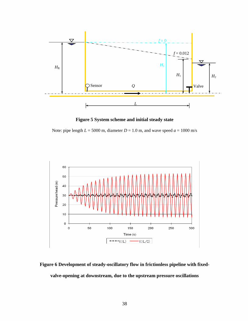
The same system, as shown in Figure 5, is studied to illustrate the application of current

mathematical model. In this system, a long horizontal pipeline links two constant head

reservoirs. At the entrance of downstream reservoir, there is a valve with constant ES = 7

m2.5/s and initial opening 0τ = 0.1. The upstream reservoir has 30 m water head initially

(HR0 = 30 m) and downstream reservoir has a constant head of 15 m. The water level at

upstream reservoir starts to fluctuate sinusoidally, which induces transient events in the

system. The amplitude of oscillatory wave is 2 m; the cyclic period is 10 s, which equals

2L/a, so that resonance would be expected to take place. The instant pressure at the

upstream reservoir can be described as:

)10/2sin(2)( 0 tHtH RR π+= (10)

17

In the first example, it is assumed the pipeline is frictionless, i.e., the Darcy-

Weisbach friction factor f = 0. At initial steady state, the hydraulic head at the valve inlet

equals the reservoir head, that is, H10 = HR0 = 30 m, and the flow rate in the system and

passing through the valve is Q0 = 2.71 m3/s.

If the downstream valve remains at its initial opening 0τ = 0.1 (i.e., fixed orifice),

the oscillations of upstream pressure (i.e., incidental pressure wave, or forced vibration)

will cause hydraulic resonance and pressure amplification in the middle part of the

pipeline. Figure 6 shows the development of the steady-oscillatory flow in the pipeline;

the red/solid line represents the pressure oscillations at the middle-point of the pipeline

and the black/dashed line represents the pressure oscillations at the valve inlet. There is a

L/2a time difference (i.e., 1/8 phase difference) between these two pressure waves, and

the amplitudes of both waves are initially small and grow gradually until they finally

stabilize at a resonance condition (within 300 s). This mode shape of the pressure waves

can be understood and explained as follows: in this system, the upstream incidental wave

will propagate along the pipeline and reach the valve inlet in 5 s (L/a = 5 s), and thus it

will take 7.5 s for the first peak of the sinusoidal wave (with the oscillatory period 10 s)

to arrive at the valve inlet. During the time period 5 to 7.5 s, the pressure at the valve

inlet, indeed at any internal pipe node, is the superposition of the incident wave and the

reflected wave from the fixed valve at downstream reservoir. Since the reflection at

downstream boundary in this case is negative, the first wave peak is reduced when it

arrives at downstream valve. However, the pressure waves with different amplitudes

would continuously proceed and be reflected. The result of superposition increases until

the maximum amplitude reached and the steady-oscillatory flow condition developed in

18

the system. This simulation result with fixed valve opening is also represented by the

red/dashed lines in Figure 7. The value of the steady amplitude at each position of

pipeline depends on the system frequency and resistance characteristics. As matter of

fact, this phenomenon resulting from the forced vibration of upstream pressure (with

fixed downstream valve opening) is equivalent to the responses caused by the periodic

valve motion at downstream end (while keeping the upstream reservoir head constant),

as summarized in Figure 8.2 on page 204 of Chaudhry (1979).

To eliminate or limit the reflection and superposition of pressure waves in the

pipeline, a sensor is installed at the upstream node, and a PID controller positioned at the

downstream valve. The constants of PID controller are taken as KC = 250, Ti = 0.002 s

and Td = 0.5 s. The total simulation time is run for 800 s, and the time step is 1/100 s that

is sufficiently small to look into the detailed valve responses.

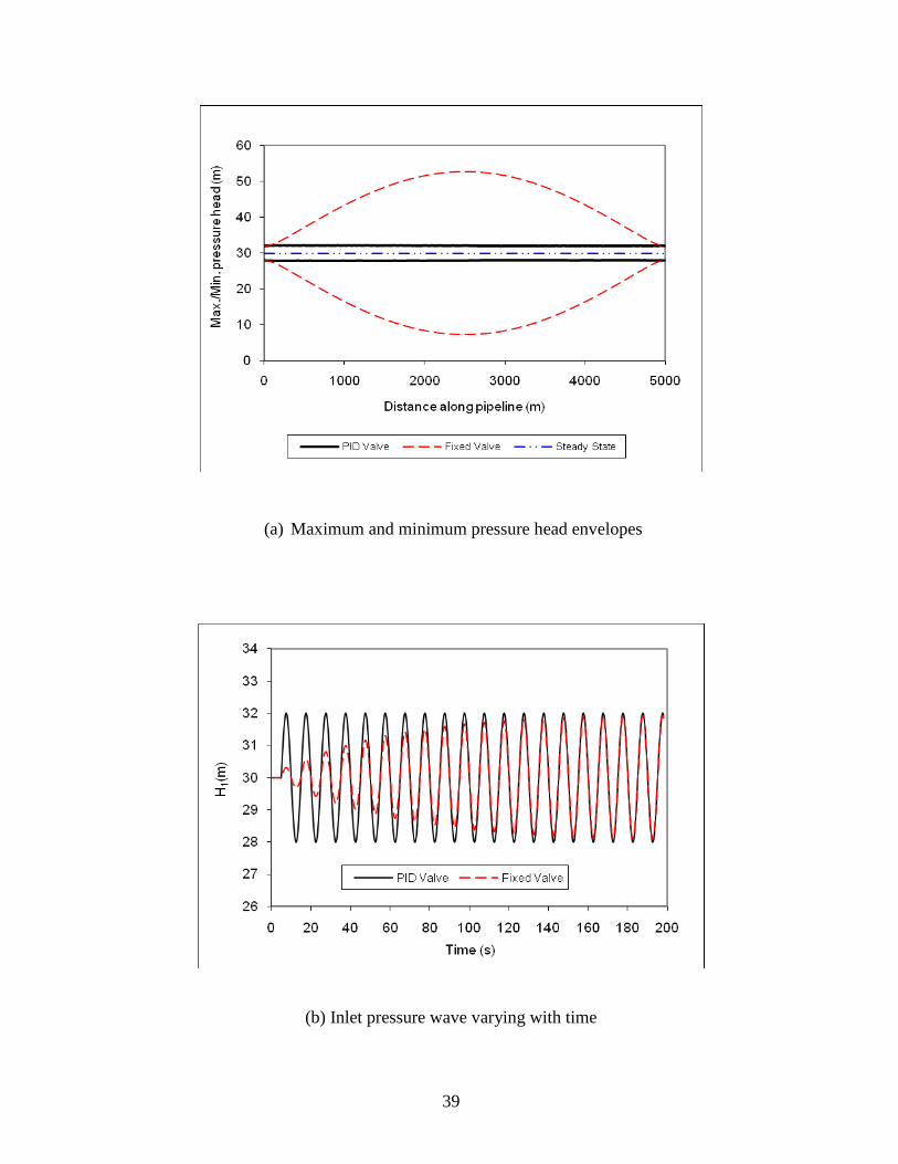
The developed remote control model for frictionless pipeline is used in this

example to simulate the system responses to the oscillations of pressure head at the

upstream reservoir. Figure 7 compares the system responses for the responsive PID

control valve (black/solid lines) and the conventional valve with fixed orifice (red/dashed

lines). The black/solid lines in Figure 7 (a) show that the maximum and minimum

pressures along the pipeline remain the same as those introduced at upstream reservoir,

demonstrating no wave reflection or resonance ever occurred in the system by using

remote sensor and PID control valve. In Figure 7 (c), the black/solid curve shows that

the opening of PID control valve is adjusted periodically in response to the oscillating

incident pressure waves, as expected, which exactly eliminates the wave reflections at

19

the valve (by exciting a contrary wave) and thus remains the same mode shape of

pressure oscillation as of the upstream incident wave, see the black/solid H1 waves in

Figure 7 (b).

By contrast, if the valve opening is fixed at the initial size ( 1.0=τ ) as the

straight red/dashed line in Figure 7 (c), the amplitude of pressure waves at the inlet of

fixed orifice reduces at the beginning and grows gradually until finally stabilized at

certain value because of resistance of the valve, as shown in the red/dashed H1 wave in

Figure 7 (b). Correspondingly, the pressure waves are reflected and superposed in the

pipeline, resulting in the increased envelope of maximum and minimum pressures along

the pipeline, see the red/dashed curves in Figure 7 (a).

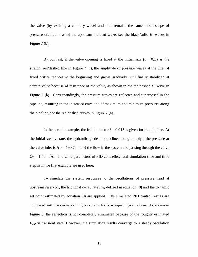
In the second example, the friction factor f = 0.012 is given for the pipeline. At

the initial steady state, the hydraulic grade line declines along the pipe, the pressure at

the valve inlet is H10 = 19.37 m, and the flow in the system and passing through the valve

Q0 = 1.46 m3/s. The same parameters of PID controller, total simulation time and time

step as in the first example are used here.

To simulate the system responses to the oscillations of pressure head at

upstream reservoir, the frictional decay rate FDR defined in equation (8) and the dynamic

set point estimated by equation (9) are applied. The simulated PID control results are

compared with the corresponding conditions for fixed-opening-valve case. As shown in

Figure 8, the reflection is not completely eliminated because of the roughly estimated

FDR in transient state. However, the simulation results converge to a steady oscillation

20

flow within 400 s, and the comparison in Figure 8 (a) shows that the maximum and

minimum pressure envelope using the PID control (solid/black curves) is smaller than

the case of fixed-opening-valve (dashed/red curves), which demonstrates the reflections

and resonance of pressure waves are constrained by using the remote sensor and PID

control valve. The smaller the initial flow in the system, the more reduction in the

magnitude of pressure amplitude envelopes, and this point can be demonstrated by the

following example with zero initial flow. Figure 8 (c) shows that the opening of the PID

control valve is adjusted periodically in response to the proceeding waves, which, as

shown in Figure 8 (b), creates a steady oscillation at the valve inlet with the same

decayed amplitude as initial steady state. Yet, for the case of fixed-opening-valve, the

amplitude of pressure waves at the valve inlet varies with time, reduced at the beginning

and increasing gradually until a steady-oscillatory flow developed over about 300 s.

5.2 Examples with Zero Initial Flow (Static Initial State)

In the system sketched in Figure 5, there is no flow in the system and the initial valve

opening is of no consequence if the constant heads (30 m) are remained at both upstream

and downstream reservoirs. Yet, if a sinusoidal oscillation of head at the upstream

reservoir is initiated, a flow in the pipeline will be created, and the flow direction shifts

as the head oscillates around the original constant level. At any specific point of the

pipeline (e.g., at the valve), the magnitude of oscillatory flow is small and the average

value with time is zero. The f value by itself seems hardly influence the wave reflection.

Therefore, for both cases with frictionless and frictional pipeline, the wave reflection and

resonance can be completely eliminated and the “non-reflective” boundary achieved at

21

the downstream valve, if the remote sensing and PID controlled valve are implemented

in the system.

Figure 9 shows the simulation results including the friction factor of 0.012.

Without the flow (and thus without resistance from flow), the resonance would be

stabilized in around 600 s for the fixed valve opening case and the range of the max./min.

pressures are much larger than that with non-zero flow case. While with responsive PID

control valve, there is no wave reflection and resonance at all in the system, and the

oscillations remain steady at any point and at any time, as the same as the upstream

incident pressure oscillations.

6. Frequency Analysis and “Non-Reflective” Boundary Verification

Based on the time domain transient analysis using method of characteristics (MOC), the

numerical model for “non-reflective” boundary design has been developed in previous

sections. However, for a periodic oscillation originating at a remote location, transient

analysis in the frequency domain is a more practical and efficient way to reveal the

oscillatory conditions in the fluid system.

In this section, oscillation is introduced through various harmonics that might

occur in the pipe system. Then, the system responses to the forced vibrations (upstream

pressure oscillations) with different frequencies and the applicability of developed “non-

reflective” model are checked. After that, the steady “non-reflective” boundary

conditions for the frictionless pipeline system, obtained by the traditional MOC, would

be verified using the method of hydraulic impedance in the frequency domain.

22

6.1 System Responses to Pressure Oscillations with Various Frequencies

Unexpected resonance could be destructive in practical hydraulic systems. The

consequences of resonance in fluid systems range from objectionable operating

conditions, such as instability, noise, and vibration, to fatal damage of system elements

overstressed during severe pressure oscillations. Thus, the phenomenon of hydraulic

resonance should be predicted and prevented.

In the example discussed in previous section, the incident pressure oscillation at

upstream reservoir is one type of forced excitation. The fundamental period of pipeline

system T0 = 4L/a = 20 s (i.e., natural frequency is 1/20 Hz) and the given period of forced

excitation T = 10 s (the forcing frequency is 1/10 Hz), and the system responses to this

forced excitation are shown in Figure 7 (a) and Figure 8 (a) for frictionless and frictional

pipeline, respectively. For a fixed orifice at downstream reservoir, the system responses

demonstrate the characters of second harmonics, and the maximum amplitude of

pressure oscillation, occurred at the middle point of the pipeline, is about 12 and 9 times

as large as the incident pressure oscillation, respectively, for frictionless and frictional

cases. Now, what if we change the frequency of the forced excitation? Could we adjust

downstream valve opening to eliminate the potential resonance in the system using the

developed “non-reflective” boundary design?

Frictionless pipeline system with non-zero initial flow. In the system with the

fixed valve opening at downstream reservoir (Figure 5), even order of harmonics exist,

as shown in Figure 10 (b), (d) and (f). The even harmonics indicates that the reflective

characteristic at downstream orifice is similar to a reservoir (negative reflection) (Wylie

23

et al. 1993 and Chaudhry 1987). This can be verified by comparing the hydraulic

impedance of the fixed valve with the characteristic impedance of the system. Hydraulic

impedance in a fluid system is defined as the ratio of the complex head to the complex

discharge at a particular point in the system (Wylie et al. 1993).

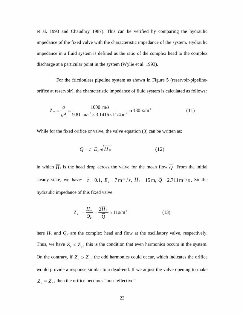
For the frictionless pipeline system as shown in Figure 5 (reservoir-pipeline-

orifice at reservoir), the characteristic impedance of fluid system is calculated as follows:

11) ( s/m 130m /411416.3m/s 9.81

m/s 1000 2222 ≈

××==

gAaZC

While for the fixed orifice or valve, the valve equation (3) can be written as:

(12) 0HEQ Sτ=

in which 0H is the head drop across the valve for the mean flow Q . From the initial

steady state, we have: . /m 711.2 m, 15 ,/m 7 0.1, 30

2.5 sQHsES ====τ So the

hydraulic impedance of this fixed valve:

(13) s/m 112 20 ≈==QH

QH

ZV

VV

here HV and QV are the complex head and flow at the oscillatory valve, respectively.

Thus, we have CV ZZ < , this is the condition that even harmonics occurs in the system.

On the contrary, if CV ZZ > , the odd harmonics could occur, which indicates the orifice

would provide a response similar to a dead-end. If we adjust the valve opening to make

CV ZZ = , then the orifice becomes “non-reflective”.

24

When the cyclic period of the forced vibration is given as fractional part of the

fundamental period (T0 = 4L/a =20 s), the different orders of harmonics and different

mode shapes of pressure waves would occur in the pipe system. However, the frequency

change doesn’t affect the amplitude of each harmonics if the amplitude of incidental

pressure oscillation remains the same. The order of harmonics equals the system

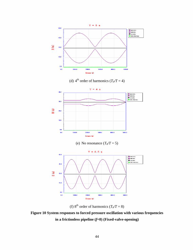
fundamental period T0 divided by the period of forced vibration T. If we give even

number of T0/T (i.e., T = 10 s, 5 s, 3.3 s, 2.5 s, ….), the excessive energy influx to the

system during oscillatory flow leads to resonance, as shown in Figure 10 (b), (d) and (f).

In an ideal lossless system (for this frictionless pipeline system the only energy

dissipation occurs at the downstream valve), there is generally no energy transmission in

steady-oscillatory flow, although alternating energy conversion between kinetic energy

and pressure energy may occur. With terminal wave reflection, steady-oscillatory motion

shows a combination of forward and reflected waves which results in a standing wave.

Within the standing-wave pattern, energy is converted from pressure energy to kinetic

energy, then back to pressure energy, and so on. If we give odd number of T0 /T (i.e., T

= 20 s, 6.67 s and 4 s,…), as shown in Figure 10 (a), (c) and (e), the mode shape of the

pressure waves is quite different from the even harmonics, the energy dissipated

gradually and resonance does not occur in the system.

It is not surprising to find that the resonance with different orders of harmonics

and amplification of pressure head can be completely eliminated in frictionless pipeline

by designing a “non-reflective” boundary. The simulated results are all the same as the

black/dotted line in Figure 7 (a), no matter how the period of the forced vibration T

changes. However, it is noticed that for the higher frequency forced oscillations (smaller

25

T), the PID integral and derivative parameters (Ti and Td) require smaller values to obtain

the precise adjustment of “non-reflective” valve opening.

Frictional pipeline system with non-zero initial flow. For the frictional

pipeline case, we have a similar finding regarding even harmonics when we change the

period of the forced vibration. The application of remote sensor and PID control valve

cannot completely eliminate the reflections and resonance if the initial flow is not zero,

but the amplitude of the pressure waves is significantly reduced for each harmonics, as

shown Figure 11. In this Figure, the different responses to the forced oscillations at the

upstream end are compared for the system with a fixed-opening-valve and responsive

PID valve at the downstream end of pipeline.

6.2 “Non-Reflective” Boundary Verification using Hydraulic Impedance Method

From the viewpoint of frequency domain, the automatically adjustable PID valve creates

an artificial excitation and the consequence of this designed valve-oscillation would

exactly cancel out the effect of incidental pressure oscillation at the upstream reservoir.

For the frictionless pipeline system, we have verified the condition of a “non-reflective”

boundary, that is, CV ZZ = , for the developed steady-oscillatory flow (i.e., after 300 s of

PID valve adjustment when the amplitude of the pressure waves in the pipeline

stabilized). This steady valve-oscillating condition has been obtained from the numerical

simulation in the time domain, which uses the “non-reflective” boundary model

developed in the previous section.

26

For the frictionless pipeline system, the characteristic impedance has been

calculated as equation (11). For an oscillating valve, the hydraulic impedance at the

upstream side of the valve can be calculated by (Wylie et al. 1993)

(14) 22 00

V

V

V

VV Q

THQH

QH Z

τ−==

We already know /m 711.2 m, 15 0.1, 30 sQH ===τ , and here HV, QV and VT are the

complex head, flow and opening at the oscillatory valve, respectively.

From numerical simulation in the time domain, as the results shown in Figure

7, we found the maximum valve opening 107.0( max =τ ) corresponding to the minimum

valve flow (Qmin = 2.695 m3/s), and minimum valve inlet head (H1min = 28.0 m). On the

contrary, the minimum valve opening 094.0 ( min =τ ), corresponds to the maximum flow

(Qmax = 2.726 m3/s) and maximum valve inlet head (H1max = 32.0 m). Here, the interesting

parts of pressure, flow and valve opening time-histories are the pure oscillatory parts of

them; and a half of the difference between the maximum and minimum values is used as

the amplitude in the following calculations. In other words, we have complex hydraulic

values:

10

2sin 2.0 10

)/( 2sin 0.2

+=

+

= πππ taLtHV (15)

10

2sin 0155.0 10

)/( 2sin 0155.0

+=

+

= πππ taLtQV (16)

27

10

2sin 0065.0

=

tTVπ (17)

It is noticed that there is a phase difference of 10/)/2( aLπ between the oscillation of

valve opening (TV) and the oscillations of valve flow (QV) and inlet head (HV). So, we

can also calculate 129≈=V

VV Q

HZ s/m2, or 13722 00 ≈−=

V

VV Q

THQH Z

τ s/m2 (from

equations (16) and (17), we know TV and QV have opposite sign; the numerical error is

acceptable due to only 3 digitals of the simulation results recorded). Therefore, the “non-

reflective” boundary condition CV ZZ ≈ =130 s/m2 has been verified.

In the case without initial flow but the pipeline with friction, as shown in

Figure 8, we obtained the same pressure and flow oscillations at the valve as described in

equations (15) and (16), and thus V

VV Q

HZ = ≈ ZC =130 s/m2 can be verified. Moreover,

by changing the amplitude of the incident pressure waves at the upstream reservoir, the

amplitude of induced flow oscillations would change proportionally, so the value of

V

VV Q

HZ = remains near 130 and “non-reflective” boundary condition would be always

achieved for static initial state cases.

To further verify this law of “non-reflective” boundary condition, the wave

speed of pipeline is reduced to 500 m/s, so the system characteristic impedance also

reduces to s/m 65 2≈=gAaZC . The “non-reflective” boundary condition, CV ZZ = , could

be verified as well by the corresponding numerical simulation results in the time domain.

28

7. Tuning PID Controller

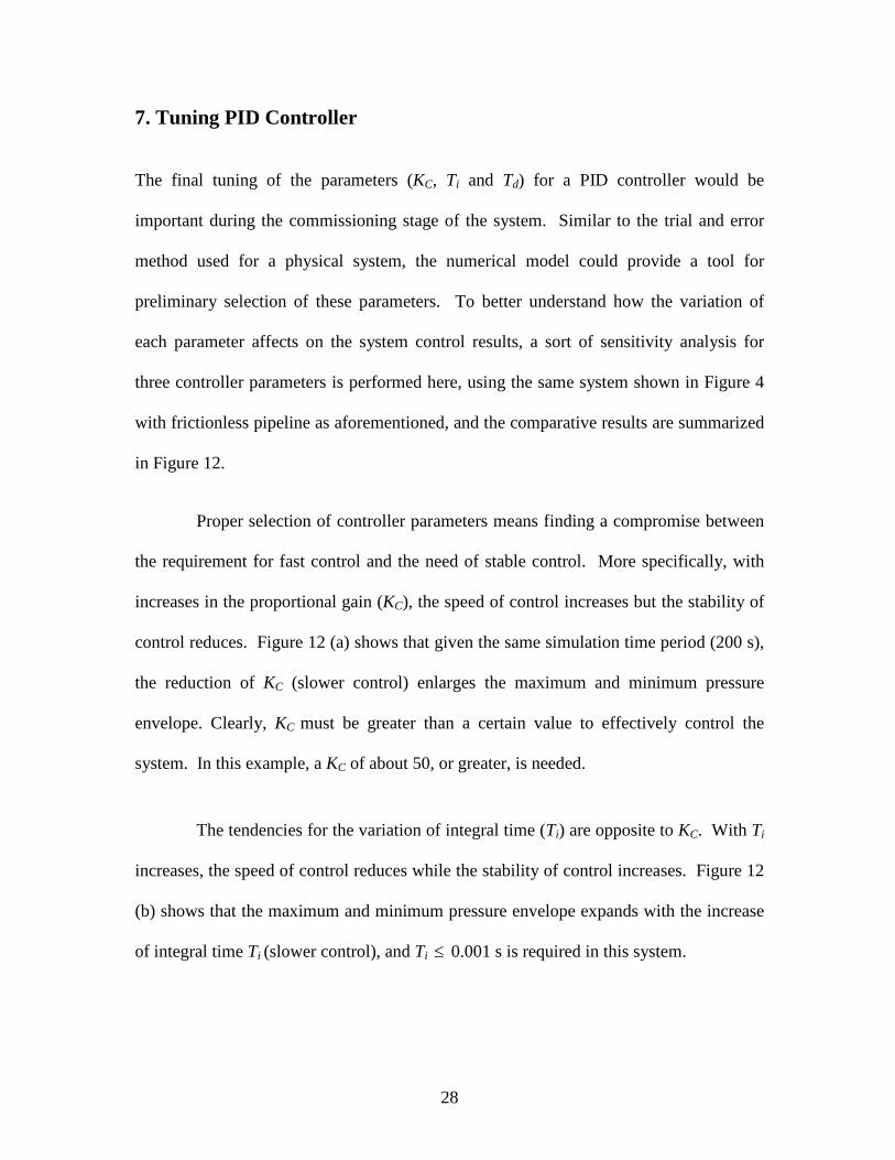
The final tuning of the parameters (KC, Ti and Td) for a PID controller would be

important during the commissioning stage of the system. Similar to the trial and error

method used for a physical system, the numerical model could provide a tool for

preliminary selection of these parameters. To better understand how the variation of

each parameter affects on the system control results, a sort of sensitivity analysis for

three controller parameters is performed here, using the same system shown in Figure 4

with frictionless pipeline as aforementioned, and the comparative results are summarized

in Figure 12.

Proper selection of controller parameters means finding a compromise between

the requirement for fast control and the need of stable control. More specifically, with

increases in the proportional gain (KC), the speed of control increases but the stability of

control reduces. Figure 12 (a) shows that given the same simulation time period (200 s),

the reduction of KC (slower control) enlarges the maximum and minimum pressure

envelope. Clearly, KC must be greater than a certain value to effectively control the

system. In this example, a KC of about 50, or greater, is needed.

The tendencies for the variation of integral time (Ti) are opposite to KC. With Ti

increases, the speed of control reduces while the stability of control increases. Figure 12

(b) shows that the maximum and minimum pressure envelope expands with the increase

of integral time Ti (slower control), and Ti ≤ 0.001 s is required in this system.

29

The derivative part produces both faster and more stable control when Td

increases. However, this is only true up to a certain limit and if the signal is sufficiently

free of noise (calculation error is a kind of noise in numerical system). If Td rises above

this limit it will result in reduced stability of control. As we know that the function of the

derivative part is to estimate the change in the control a time Td ahead. This estimate will

naturally be poor for large values of Td. Another consideration is the noise and other

disturbances. The noise is amplified to a greater extent when Td increases, and thus it is

often the noise that sets the upper limit for the magnitude of Td. The above theoretical

analysis could be verified by the numerical simulations in Figure 12 (c), which shows

that the control stability is better when Td = 0.5 s (dashed lines) than that when Td =

0.005 s (dot-dash lines). However, when Td = 5 s the stability of control is poor.

In addition, the simulations also show that for high frequency oscillatory flow

(e.g., 1 s of the period of incidental pressure wave), the smaller values for both the

integral time constant Ti and derivative time constant Td are required.

The stability and speed of control process are associated with the parameters of

controller. The mathematical model and numerical simulation are useful for selection

and tuning of the controller parameters, which could save time and cost in

commissioning of the physical system.

8. Conclusion and Discussion

The creation of “non-reflective” (or “semi-reflective”) boundaries through remote

sensing and PID control valve is a new concept to more accurately limit dead-end

30

reflection and resonance in pipelines. This idea is explored here by the means of

numerical simulation, and a considerable potential for transient protection has been

demonstrated in the numerical examples. As shown, wave reflection and resonance can

possibly be eliminated for frictionless pipelines or the pipelines with static initial states;

while for the pipeline with some friction, the pressure waves’ reflection at the valve and

superposition within the pipeline can be effectively limited. Moreover, the feature of

even order of harmonics as well as “non-reflective” boundary conditions during steady

oscillation, obtained through time domain transient analysis, are verified by hydraulic

impedance analysis in the frequency domain. Certainly dead-end branches are a common

component in pipe networks; at such locations, dead-end reflection may cause

unexpected high pressures when system experiences transients, and such locations might

readily be improved with appropriate thought to tailored wave reflections such as those

described in this paper.

However, complications and challenges will inevitably arise when the model

of “non-reflective” boundary is applied in practice. First, the model is developed based

on a single pipeline system with the remote sensor at upstream end and PID control valve

at downstream end. It is feasible to apply the model for a branched pipeline in a complex

system with remote sensor at the junction and a terminal valve at the branch-end, but

further application to a pipe loop or an arbitrary pipeline with other components between

the two ends would be significantly challenging, since the primary pressure wave would

be reflected, refracted, or attenuated by those components and thus the theoretical

estimate of pressure set point become almost impossible. Besides, in real systems, the

uncertainties (including entrapped air effect or frequency-relevance) in the magnitudes of

31

waves speed, pipe friction factor and pressure decay rate at transient state may cause

significant over- or under-estimate of pressure set point and thus require for careful

system calibrations in advance. The upstream pressure disturbance may not be a steady

oscillation as in the real systems, and then the reflections at the upstream reservoir would

further complicate the “non-reflective” valve opening control. Thus, at present the design

of “non-reflective” boundary, though promising, calls for considerable further research

as and likely will require cooperation with device manufacturers.

References

Almeida A. B. de and Koelle E. (1992). “Fluid Transients in Pipe Networks. ” Co-

published by Computational Mechanics Publications, Southampton Boston and

Elsevier Science Publishers Ltd., London New York, 111-112.

Bounce B. and Morelli L. (1999). “Automatic control valve-induced transients in

operative pipe system.” J. of Hydraulic Engineering, ASCE, 125(5), 543-542.

Chaudhry M. Hanif (1979). “Applied Hydraulic Transients.” Van Nostrand Reinhold

Company, New York.

Hopkins John P. (1998). “Valves for controlling pressure, flow and level.” J. of Water

Engineering & Management, 135(8), 42.

Karney B.W. and McInnis D.A. (1992). “Efficient calculation of transient flow in simple

pipe networks.” J. of Hydr. Engrg., ASCE, 118(7), 1014-1030.

32

Koelle E. (1992). “Control valves inducing oscillatory flow in hydraulic networks.”

Proc., International Conference on Unsteady Flow and Fluid Transients, Durham,

United Kingdom, 343-352.

Koelle E. and Poll H. (1992). “Dynamic behavior of automatic control valves (ACV) in

hydraulic networks.” Proc., 16th Symposium of the IAHR – Section on Hydraulic

Machinery and Cavitation, Sao Paulo, Brazil, 127-139.

Lauria J. and Koelle E. (1996). “Model-based analysis of active PID-control of transient

flow in hydraulic networks.” Hydraulic Machinery and Cavitation, Kluwer

Academic Publishers, printed in the Netherlands, 749-758

Poll H. (2002). “The importance of the unsteady friction term of the momentum equation

for hydraulic transients.” Proc., 21st IAHR Symposium on Hydraulic Machinery

and Systems, Lausanne, Switzerland.

Suzuki, K., Taketomi, T., and Sato, S. (1991). “Improving Zielke’s Method of

Simulating Frequency-Dependent Friction in Laminar Liquid Pipe Flow.” Journal

of Fluids Engineering, Transaction of the ASME, Vol. 113, 569-573.

Tan Kok Kiong, Wang Quing-Guo, Hang Chang Chieh and Tore J. Hagglund (1999).

“Advances in PID Control.” Springer-Verlag London Ltd., London, UK.

Tirkha, A. K. (1975). “An efficient method for simulating frequency-dependent friction

in transient liquid flow.” Journal of Fluids Engineering, Transactions of the

ASME, March, 97-105.

33

Vardy, A. E., Hwang, K., and Brown, J. M. B. (1993). “A weighting function model of

transient turbulent pipe friction.” Journal of Hydraulic Research, Vol. 31 (4), 533-

548.

Vardy, A. E. and Brown, J. M. B. (1995). “Transient, Turbulent, Smooth Pipe Friction.”

Journal of Hydraulic Research, Vol. 33 (4), 435-456.

Vardy, A. E. and Brown, J. M. B. (2003). “Transient Turbulent Friction in Smooth Pipe

Flows.” Journal of Sound and Vibration, Vol. 259 (5), 1011-1036.

Wylie E. B., Streeter V. L. and Suo L. (1993). “Fluid Transients in Systems.” Prentice-

Hall Inc., Englewood Cliffs, New Jersey.

Zielke, W. (1986). “Frequency-dependent friction in transient pipe flow.” Journal of

Basic Engineering, Transactions of the ASME, Vol. 90 (1), 109-115.

34

Figure 1 Scheme of a branched system and initial pressure head

Note: Pipe length AB = BC = CD = DE = CF = DG = 1000 m, friction factor f = 0.012, the

diameter of main pipeline D = 1 m, and the diameter of branches d = 0.5 m. Initially, the terminal

control valves at the end of branches are fully closed. If the pipes do not leak and have been open

to the reservoirs for some time, no flow will occur in the system and the head will be uniformly

100 m as found in the reservoirs. Following Boulos et al. (2006), suppose the second section of

the main pipeline (from B to C) is pressurized to a uniform value of 130 m.

100 m 100 m

80

130 m

A B C D

F G

35

(a) Transient response in the system with dead-end branches

(b) Transient response in the system with 10% orifices at branch ends

(c) Transient response in the system with 0.35% orifices at branch ends

Figure 2 Comparison of transient responses to dead-ends and small orifices

Max. H

Min. H

Initial H Pipeline

A B C F

Max. H

Min. H

Initial H

Pipeline

A B C F

Max. H

Min. H

Initial H

Pipeline

A B C F

36

Figure 3 Traveling pulse waves and “tailored” valve reflections

Valve Opening=10% Valve Opening=20%

Valve Opening=30% Valve Opening=60%

Valve Opening=0%

Valve Opening=100%

37

Figure 4 PID-controlled valve in a pipe network

Q Node2 Node1 Pipe

Pipe

Q

Pipe

Pipe

H1

H2

H

38

HR

Valve Sensor Q

L

H1 H2

f = 0

f = 0.012

H1

Figure 5 System scheme and initial steady state

Note: pipe length L = 5000 m, diameter D = 1.0 m, and wave speed a = 1000 m/s

Figure 6 Development of steady-oscillatory flow in frictionless pipeline with fixed-

valve-opening at downstream, due to the upstream pressure oscillations

39

(a) Maximum and minimum pressure head envelopes

(b) Inlet pressure wave varying with time

40

(c) Valve opening varying with time

Figure 7 Responsive PID control valve vs. fixed-opening-valve in frictionless pipeline (f=0)

(a) Maximum and minimum pressure head envelopes

41

(b) Inlet pressure wave varying with time

(c) Valve opening varying with time

Figure 8 Responsive PID control valve vs. fixed-opening-valve

in frictional pipeline (f=0.012)

42

(a) Maximum and minimum pressure head envelopes

(b) Inlet pressure wave and flow at the PID valve varying with time

Figure 9 Responsive PID control valve vs. fixed-opening-valve for static initial states

with frictional pipeline (f=0.012)

H1

Q

43

(a) No resonance (T0/T = 1)

(b) 2nd order of harmonics (T0/T = 2)

(c) No resonance (T0/T = 3)

44

(d) 4th order of harmonics (T0/T = 4)

(e) No resonance (T0/T = 5)

(f) 8th order of harmonics (T0/T = 8)

Figure 10 System responses to forced pressure oscillation with various frequencies

in a frictionless pipeline (f=0) (Fixed-valve-opening)

45

(a) t=10 s

(b) t=5 s

46

(c) t=2 s

(d) t=1 s

Figure 11 System responses to forced pressure oscillation with various frequencies

in a frictional pipeline (f=0.012) (Fixed valve vs. responsive PID valve)

47

(a) Max./Min. pressure envelopes expanding with reduction of proportional gain KC

(Ti = 0.001 s, Td = 0.5 s)

(b) Max./Min. pressure envelopes expanding with increase of integral time Ti

(KC = 250, Td = 0.5 s)

Max. H

Min. H

S. S. H

Max. H

Min. H

S. S. H

48

(c) Max./Min. pressure envelopes varying with different derivative time Td

(KC = 250, Ti = 0.02 s)

Figure 12 Effect of controller parameters on system pressure control

Max. H

Min. H

S. S. H

49

Figure Captions

Figure 1 Scheme of a branched system and initial pressure head

Figure 2 Comparison of transient responses to dead-ends and small orifices

Figure 3 Traveling pulse waves and “tailored” valve reflections

Figure 4 PID-controlled valve in a pipe network

Figure 5 Examples: System scheme and initial steady state

Figure 6 Development of steady-oscillatory flow in frictionless pipeline with fixed-

valve-opening at downstream, due to the upstream pressure oscillations

Figure 7 Responsive PID control valve vs. fixed-opening-valve in frictionless pipeline

(f=0)

Figure 8 Responsive PID control valve vs. fixed-opening-valve in frictional pipeline

(f=0.012)

Figure 9 Responsive PID control valve vs. fixed-opening-valve for static initial states

with frictional pipeline (f=0.012)

Figure 10 System responses to forced pressure oscillation with various frequencies in a

frictionless pipeline (f=0)

Figure 11 System responses to forced pressure oscillation with various frequencies in a

frictional pipeline (f=0.012) (Fixed valve vs. responsive PID control valve)

Figure 12 Effect of controller parameters on system pressure control

50

Notation

a – wave speed

D – diameter of pipe cross section

e – control error or deviation of the process variable u(t) from its set point u*;

dimensionless error is defined as *)(1

utue −= .

ES – a valve size parameter determined by the energy dissipation potential of the valve.

0

0

HQ

ES∆

= (in SI unit of m2.5/s, but valve manufacturers typically report ES in units of

psiUSgpm ).

f – Darcy-Weisbach friction factor

FDR –Relative Friction Decay Rate, which is defined as the ratio of pressure heads at the

valve inlet (H10) and at the remote sensor (HR0):0

10

RDR H

HF =

H or H(t) – instant pressure head

H1 or H 1(t) – instant pressure head at valve inlet

H10 – the initial pressure head at valve inlet

H1*(t) – the dynamic set point of the pressure head at valve inlet H1(t) H2 or H2(t) – instant pressure head at valve outlet

HR or HR(t)– instant pressure head at reservoir

HR0 – the initial pressure head at reservoir

KC – the proportional gain of controller

L – pipe length

Q or Q(t) – instant flow in pipeline or passing through a valve Q0 – initial steady state flow in pipe system or passing through a valve

∆H0 – pressure head difference across a valve at initial steady state

∆H or ∆H(t) – instant pressure head difference across a valve

t – time

Ti –integral time constant of controller

Td – derivative time constant of controller

u(t) – process variable to be controlled

u* – set point or desired value of process variable

τ – Dimensionless valve opening