Embed Size (px)
DESCRIPTION
scia engineer Nonlinear and Stability 2013
Citation preview

7/18/2019 Nonlinear and Stability 2013
http://slidepdf.com/reader/full/nonlinear-and-stability-2013 1/106
Advanced Concept trainingNon Linear and Stabil ity

7/18/2019 Nonlinear and Stability 2013
http://slidepdf.com/reader/full/nonlinear-and-stability-2013 2/106
7/18/2019 Nonlinear and Stability 2013
http://slidepdf.com/reader/full/nonlinear-and-stability-2013 3/106
Table of contents
3
Contents 1. Introduction ........................................................................................................................ 1
1.1. Professional training ............................................................................................................... 1 1.2. Introduction to non linear and stability ................................................................................. 1
2.
Non-Linear behaviour of Structures ................................................................................ 2
2.1. Type of Non Linearity ................................................................................................................. 2 2.2. Non Linear Combinations .......................................................................................................... 2
3. Geometrical Non-Linearity – also possible with Concept edition ................................ 4 3.1. Overview ...................................................................................................................................... 5 3.2. Alpha critical ............................................................................................................................... 7 3.3. Imperfections .............................................................................................................................. 8
3.3.1. Global frame imperfection ϕ ................................................................................................. 9 3.3.2 Initial bow imperfection e0 .................................................................................................... 14 3.3.3. Example Global + Bow imperfection .................................................................................. 19
3.4. The second order calculation .................................................................................................. 22 3.4.1. Timoshenko ........................................................................................................................ 22 3.4.2. Newton-Raphson ................................................................................................................ 27
4. Physical Non-Linearity .................................................................................................... 33 4.1 Plastic Hinges for Steel Structures .......................................................................................... 33 4.2 Physical Non-Linear analysis for Concrete Structures ......................................................... 35
5. Local Non-Linearity ......................................................................................................... 36 5.1. Beam Local Nonlinearity – also available in the concept edition ........................................ 36
5.1.1 Members defined as Pressure only / Tension only ............................................................. 37 5.1.2 Members with Limit Force ................................................................................................... 40 5.1.3 Members with gaps.............................................................................................................. 42
5.2. Beam Local Nonlinearity including Initial Stress .................................................................. 42 5.2.1 Members with Initial Stress .................................................................................................. 44 5.2.2 Cable Elements – Not available in the Professional edition ................................................ 46
5.3. Non-Linear Member Connections ........................................................................................... 55 5.4. Support Nonlinearity ................................................................................................................ 58
5.4.1. Tension only / Pressure only Supports ............................................................................... 59 5.4.2 Nonlinear Springs for Supports ........................................................................................... 61 5.4.3 Friction Supports .................................................................................................................. 66
5.5 2D Elements ............................................................................................................................... 70 5.5.1 2D Membrane Elements – Not in Professional Edition ....................................................... 70 5.5.2. Pressure only ...................................................................................................................... 74
6. Stability Calculations ...................................................................................................... 78 6.1 Stability Combinations ............................................................................................................ 78 6.2 Linear Stability ........................................................................................................................ 78 6.3 Non-Linear Stability ................................................................................................................ 94
7. Troubleshooting ..................................................................................................................... 99 7.1 Singularity ............................................................................................................................... 99 7.2 Convergence .......................................................................................................................... 99
8. References ..................................................................................................................... 101

7/18/2019 Nonlinear and Stability 2013
http://slidepdf.com/reader/full/nonlinear-and-stability-2013 4/106
7/18/2019 Nonlinear and Stability 2013
http://slidepdf.com/reader/full/nonlinear-and-stability-2013 5/106
Advanced Training
1
1. Introduction
1.1. Professional training
This course will explain the non linear and stability calculations in Scia Engineer. Most of the modules
necessary for this calculation are included in the Professional edition.For some options a concept edition is sufficient or for other options an expert edition or an extramodule is required. This will always be indicated in the corresponding paragraph.
1.2. Introduction to non linear and stability
In general, when modelling structures, a linear approach is followed. It can however be that certainparts of the structure do not behave linearly. Examples include supports or members which only act incompression or tension. This is where non-linear analysis is required.
Another example is when performing structural analysis following the latest codes (i.e. Eurocode 3).When performing manual calculations, in most cases a linear 1st Order analysis is carried out.
However, the assumptions of such analysis are not always valid and the codes then advise the use of2nd
Order analysis, imperfections, etc.
Scia Engineer contains specialized modules covering non-linear and stability related issues. In thiscourse, the different aspects of these modules are regarded in detail.
In the first part of the course, the non-linear modules are looked upon. First the 2nd
Order calculationmethods are explained and integrated with Eurocode 3. Next the local nonlinearities are examinedincluding tension-only members, pressure-only supports, cable analysis, friction supports, etc.
The non-linear part of the course is finished with an insight on how to apply imperfections according toEurocode 3 using Scia Engineer.
The second part of the course examines Stability calculations: the determination of the elastic criticalbuckling load of a structure. This analysis can be used to calculate the buckling length of a part of thestructure or to determine if a 1
st Order analysis may be carried out.
The final chapter provides some common failure messages which occur during a non-linear analysis.This chapter points out the most likely causes of singularities and convergence failures.
7/18/2019 Nonlinear and Stability 2013
http://slidepdf.com/reader/full/nonlinear-and-stability-2013 6/106
Non linear and Stability
2
2. Non-Linear behaviour of Structures
2.1. Type of Non Linearity
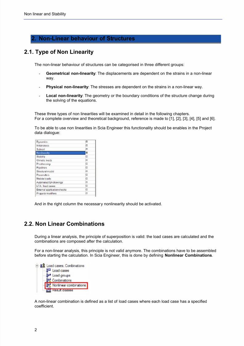
The non-linear behaviour of structures can be categorised in three different groups:
- Geometrical non-linearity: The displacements are dependent on the strains in a non-linearway.
- Physical non-linearity: The stresses are dependent on the strains in a non-linear way.
- Local non-linearity: The geometry or the boundary conditions of the structure change duringthe solving of the equations.
These three types of non linearities will be examined in detail in the following chapters.For a complete overview and theoretical background, reference is made to [1], [2], [3], [4], [5] and [6].
To be able to use non linearities in Scia Engineer this functionality should be enables in the Projectdata dialogue:
And in the right column the necessary nonlinearity should be activated.
2.2. Non Linear Combinations
During a linear analysis, the principle of superposition is valid: the load cases are calculated and the
combinations are composed after the calculation.
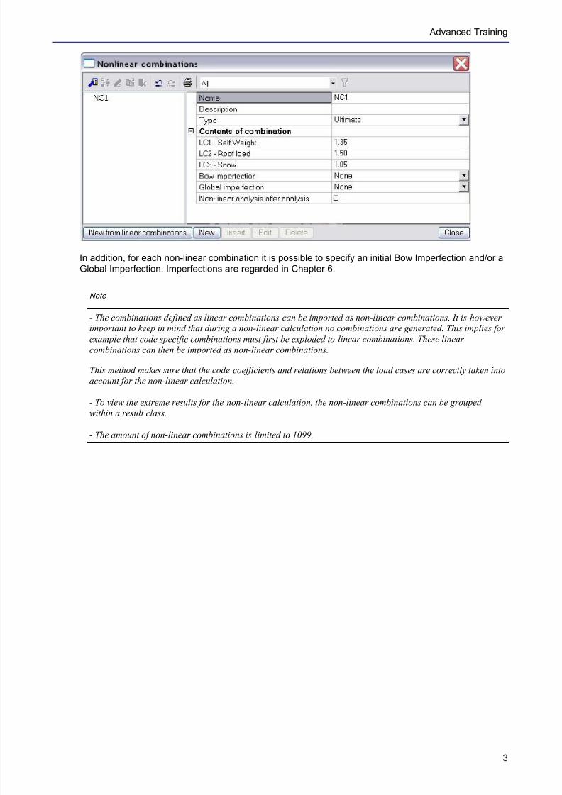
For a non-linear analysis, this principle is not valid anymore. The combinations have to be assembledbefore starting the calculation. In Scia Engineer, this is done by defining Nonlinear Combinations.
A non-linear combination is defined as a list of load cases where each load case has a specifiedcoefficient.
7/18/2019 Nonlinear and Stability 2013
http://slidepdf.com/reader/full/nonlinear-and-stability-2013 7/106
Advanced Training
3
In addition, for each non-linear combination it is possible to specify an initial Bow Imperfection and/or aGlobal Imperfection. Imperfections are regarded in Chapter 6.
Note
- The combinations defined as linear combinations can be imported as non-linear combinations. It is howeverimportant to keep in mind that during a non-linear calculation no combinations are generated. This implies for
example that code specific combinations must first be exploded to linear combinations. These linear
combinations can then be imported as non-linear combinations.
This method makes sure that the code coefficients and relations between the load cases are correctly taken intoaccount for the non-linear calculation.
- To view the extreme results for the non-linear calculation, the non-linear combinations can be grouped
within a result class.
- The amount of non-linear combinations is limited to 1099.

7/18/2019 Nonlinear and Stability 2013
http://slidepdf.com/reader/full/nonlinear-and-stability-2013 8/106
Non linear and Stability
4
3. Geometrical Non-Linearity – also possible with Concept edition
The options described here for the geometrical non linearities are also possible with a Conceptedition. So the Professional edition is not required for this chapter, except for the stability calculation
(and the calculation of αcr as explained shortly in this chapter).
The non-linear behaviour is caused by the magnitude of the deformations.
Take for example a simple beam: during a linear analysis, the relative deformation of the end nodes, inthe direction of the beam axis is dependent on the strain of the beam.
Due to a curvature of the beam, the distance between the end nodes is changed also. This implicatesthat the total strain is now not solely dependent on the displacement.
This relation can now be looked upon for different cases:
a) Small displacements, small rotations and small strains;
b) Large displacements, Large rotations and small strains;
c) Large displacements, Large rotations and Large strains;
In Scia Engineer, methods a) and b) have been implemented for the analysis of geometrical non-linearstructures. Method c) is less common in structural applications (for example rubber).
Method a) is called the Timoshenko method; method b) is called the Newton-Raphson method.
To activate the Geometrical Non-Linearity, the functionality Nonlinearity > 2nd
Order – Geometricalnonlinearity must be activated.
7/18/2019 Nonlinear and Stability 2013
http://slidepdf.com/reader/full/nonlinear-and-stability-2013 9/106
Advanced Training
5
3.1. Overview
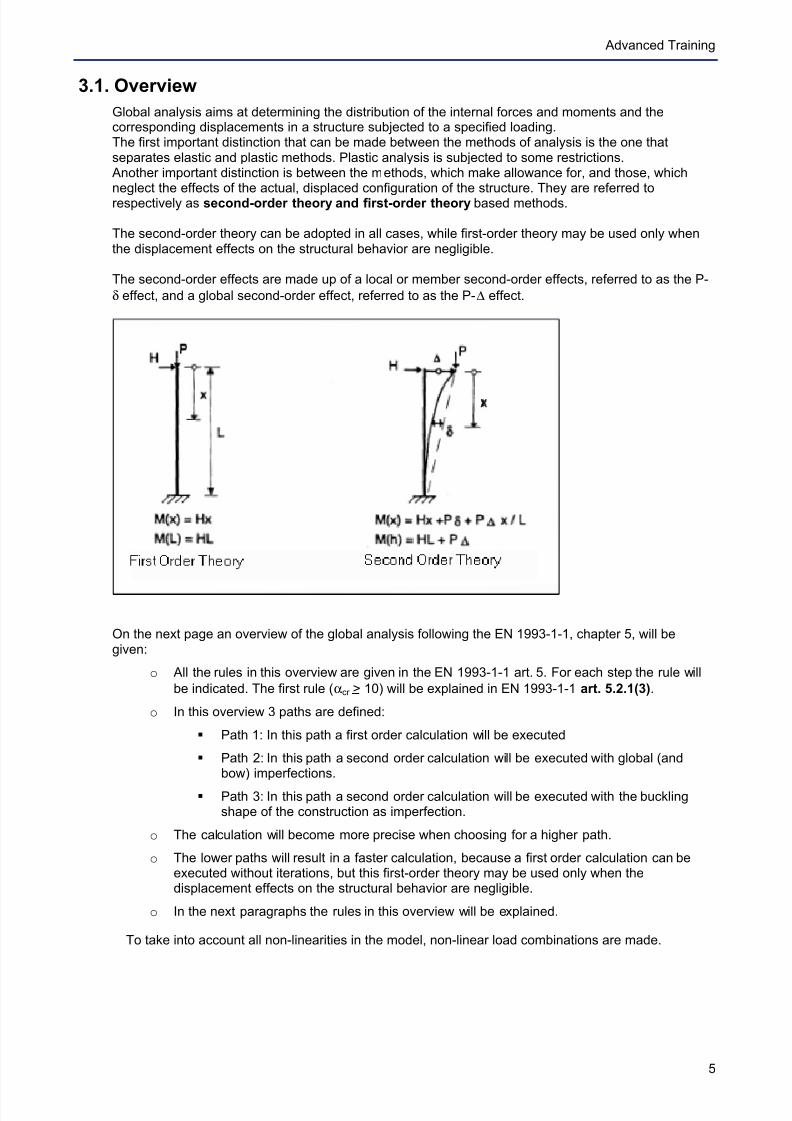
Global analysis aims at determining the distribution of the internal forces and moments and thecorresponding displacements in a structure subjected to a specified loading.The first important distinction that can be made between the methods of analysis is the one thatseparates elastic and plastic methods. Plastic analysis is subjected to some restrictions.
Another important distinction is between the methods, which make allowance for, and those, whichneglect the effects of the actual, displaced configuration of the structure. They are referred torespectively as second-order theory and first-order theory based methods.
The second-order theory can be adopted in all cases, while first-order theory may be used only whenthe displacement effects on the structural behavior are negligible.
The second-order effects are made up of a local or member second-order effects, referred to as the P-
δ effect, and a global second-order effect, referred to as the P-∆ effect.
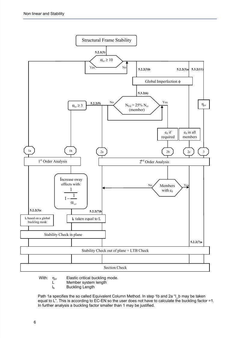
On the next page an overview of the global analysis following the EN 1993-1-1, chapter 5, will begiven:
o All the rules in this overview are given in the EN 1993-1-1 art. 5. For each step the rule will
be indicated. The first rule (αcr > 10) will be explained in EN 1993-1-1 art. 5.2.1(3).
o In this overview 3 paths are defined:
§ Path 1: In this path a first order calculation will be executed
§ Path 2: In this path a second order calculation will be executed with global (andbow) imperfections.
§ Path 3: In this path a second order calculation will be executed with the bucklingshape of the construction as imperfection.
o The calculation will become more precise when choosing for a higher path.
o The lower paths will result in a faster calculation, because a first order calculation can beexecuted without iterations, but this first-order theory may be used only when thedisplacement effects on the structural behavior are negligible.
o In the next paragraphs the rules in this overview will be explained.
To take into account all non-linearities in the model, non-linear load combinations are made.
7/18/2019 Nonlinear and Stability 2013
http://slidepdf.com/reader/full/nonlinear-and-stability-2013 10/106
Non linear and Stability
6
5.2.2(3)c
5.2.2(3)b
5.2.2(5)
5.2.2(7)b
5.3.2(11)
5.2.2(7)a
5.2.2(3)a
5.3.2(6)
5.2.1(3)
No Yes
No Yes
e0 if
required
e0 in all
members
Yes No
αcr ≥ 10
NEd > 25% Ncr
(member)
Members
with e0
αcr ≥ 3
Increase sway
effects with:
cr α
11
1
−
ηcr
1b 2b 2c 3
Global Imperfection φ
2a1a
1st Order Analysis 2
d Order Analysis
l taken equal to L
Structural Frame Stability
Section Check
Stability Check in plane
Stability Check out of plane + LTB Check
l b based on a global
buckling mode
With: ηcr Elastic critical buckling mode.L Member system lengthlb Buckling Length
Path 1a specifies the so called Equivalent Column Method. In step 1b and 2a “l_b may be takenequal to L”. This is according to EC-EN so the user does not have to calculate the buckling factor =1.In further analysis a buckling factor smaller than 1 may be justified.
7/18/2019 Nonlinear and Stability 2013
http://slidepdf.com/reader/full/nonlinear-and-stability-2013 11/106
Advanced Training
7
3.2. Alpha critical
The calculation of alpha critical is done by a stability calculation in Scia Engineer. For this calculation aProfessional or an Expert edition is necessary, so with the concept edition is this not possible. Thestability calculation has been inputted in module esas.13.
According to the EN 1993-1-1, 1st Order analysis may be used for a structure, if the increase of therelevant internal forces or moments or any other change of structural behaviour caused bydeformations can be neglected. This condition may be assumed to be fulfilled, if the following criterionis satisfied:!" =
#$%&'( ) 10 for elastic analysis
With: cr : the factor by which the design loading has to be increasedto cause elastic instability in a global mode.
FEd: the design loading on the structure.Fcr : the elastic critical buckling load for global instability,
based on initial elastic stiffnesses.
If cr has a value lower then 10, a 2nd Order calculation needs to be executed. Depending on the typeof analysis, both Global and Local imperfections need to be considered.
EN1993-1-1 prescribes that 2nd
Order effects and imperfections may be accounted for both by theglobal analysis or partially by the global analysis and partially through individual stability checks ofmembers.
The calculation of Alpha critical and also Path 3 from the diagram of the previous paragraph will beexplained in the chapter “Stability”.
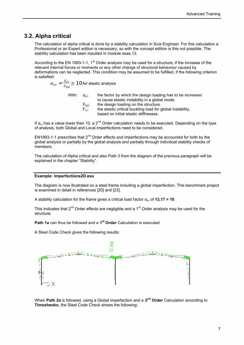
Example: Imperfections2D.esa
The diagram is now illustrated on a steel frame including a global imperfection. This benchmark projectis examined in detail in references [20] and [23].
A stability calculation for the frame gives a critical load factor cr of 13,17 > 10
This indicates that 2nd
Order effects are negligible and a 1st Order analysis may be used for the
structure.
Path 1a can thus be followed and a 1st
Order Calculation is executed.
A Steel Code Check gives the following results:
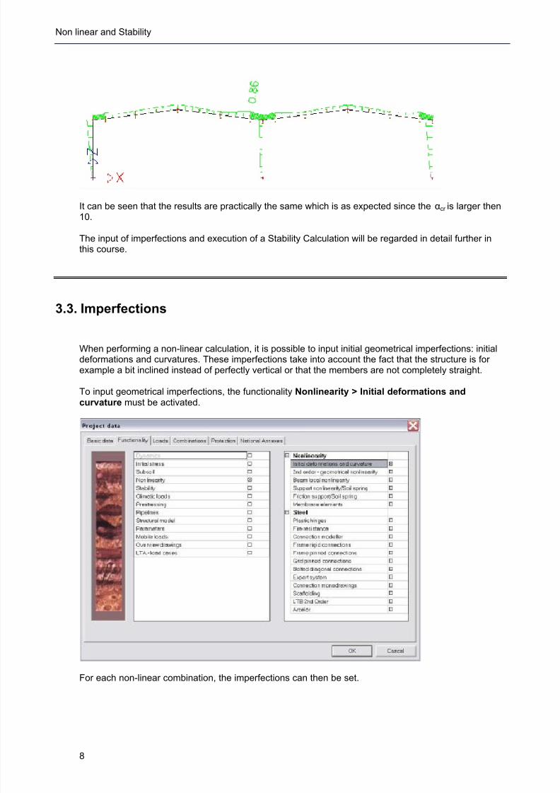
When Path 2a is followed, using a Global imperfection and a 2
nd
Order Calculation according toTimoshenko, the Steel Code Check shows the following:
7/18/2019 Nonlinear and Stability 2013
http://slidepdf.com/reader/full/nonlinear-and-stability-2013 12/106
Non linear and Stability
8
It can be seen that the results are practically the same which is as expected since the cr is larger then10.
The input of imperfections and execution of a Stability Calculation will be regarded in detail further inthis course.
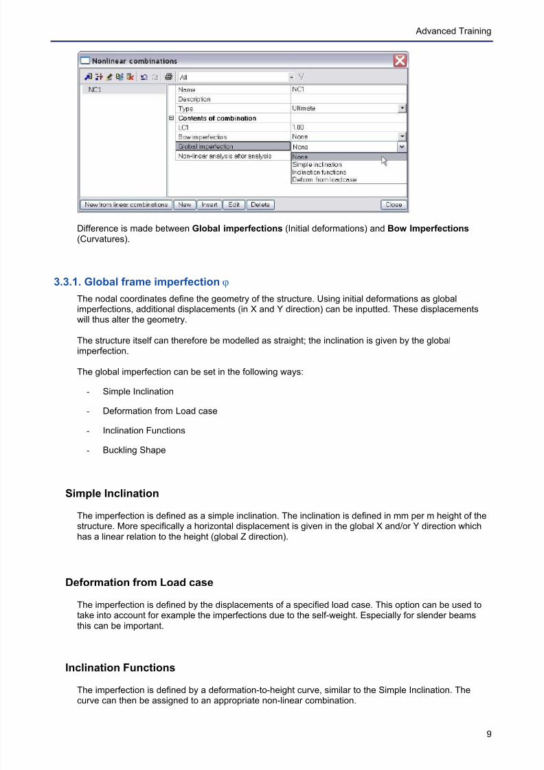
3.3. Imperfections
When performing a non-linear calculation, it is possible to input initial geometrical imperfections: initialdeformations and curvatures. These imperfections take into account the fact that the structure is forexample a bit inclined instead of perfectly vertical or that the members are not completely straight.
To input geometrical imperfections, the functionality Nonlinearity > Initial deformations andcurvature must be activated.
For each non-linear combination, the imperfections can then be set.
7/18/2019 Nonlinear and Stability 2013
http://slidepdf.com/reader/full/nonlinear-and-stability-2013 13/106
Advanced Training
9
Difference is made between Global imperfections (Initial deformations) and Bow Imperfections (Curvatures).
3.3.1. Global frame imperfection ϕ
The nodal coordinates define the geometry of the structure. Using initial deformations as globalimperfections, additional displacements (in X and Y direction) can be inputted. These displacementswill thus alter the geometry.
The structure itself can therefore be modelled as straight; the inclination is given by the globalimperfection.
The global imperfection can be set in the following ways:
- Simple Inclination
- Deformation from Load case
- Inclination Functions
- Buckling Shape
Simple Inclination
The imperfection is defined as a simple inclination. The inclination is defined in mm per m height of thestructure. More specifically a horizontal displacement is given in the global X and/or Y direction which
has a linear relation to the height (global Z direction).
Deformation from Load case
The imperfection is defined by the displacements of a specified load case. This option can be used totake into account for example the imperfections due to the self-weight. Especially for slender beamsthis can be important.
Inclination Functions
The imperfection is defined by a deformation-to-height curve, similar to the Simple Inclination. Thecurve can then be assigned to an appropriate non-linear combination.
7/18/2019 Nonlinear and Stability 2013
http://slidepdf.com/reader/full/nonlinear-and-stability-2013 14/106
Non linear and Stability
10
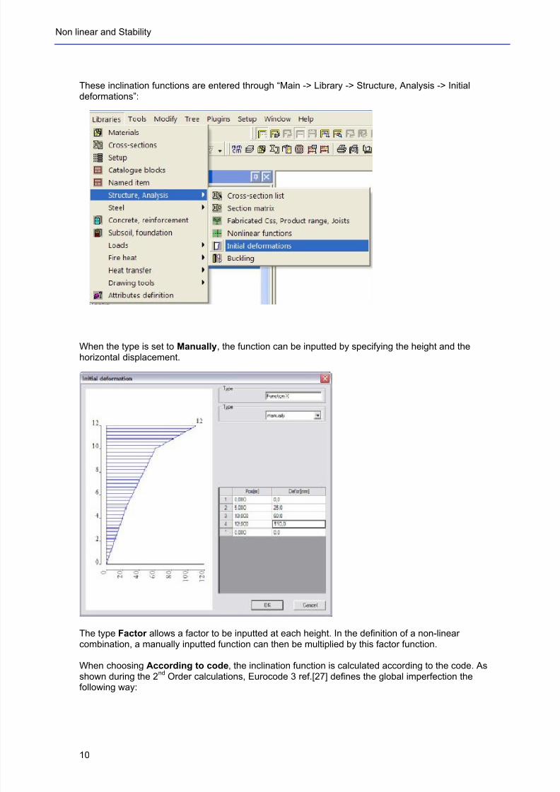
These inclination functions are entered through “Main -> Library -> Structure, Analysis -> Initialdeformations”:
When the type is set to Manually, the function can be inputted by specifying the height and thehorizontal displacement.
The type Factor allows a factor to be inputted at each height. In the definition of a non-linearcombination, a manually inputted function can then be multiplied by this factor function.
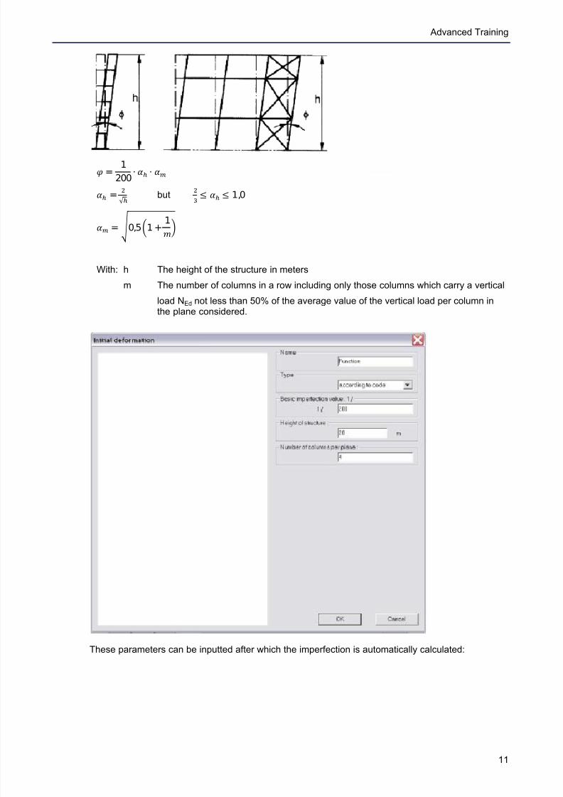
When choosing According to code, the inclination function is calculated according to the code. Asshown during the 2
nd Order calculations, Eurocode 3 ref.[27] defines the global imperfection the
following way:
7/18/2019 Nonlinear and Stability 2013
http://slidepdf.com/reader/full/nonlinear-and-stability-2013 15/106
Advanced Training
11
* =1
200+ ,- + ./
01 = 23 4 but
56 7 89 7 1,0
:; = < 0,5=1 +1>?
With: h The height of the structure in meters
m The number of columns in a row including only those columns which carry a vertical
load NEd not less than 50% of the average value of the vertical load per column inthe plane considered.
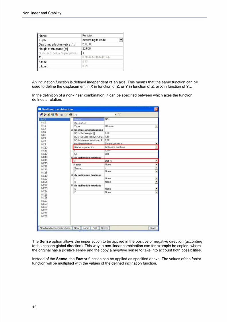
These parameters can be inputted after which the imperfection is automatically calculated:
7/18/2019 Nonlinear and Stability 2013
http://slidepdf.com/reader/full/nonlinear-and-stability-2013 16/106
Non linear and Stability
12
An inclination function is defined independent of an axis. This means that the same function can beused to define the displacement in X in function of Z, or Y in function of Z, or X in function of Y,…
In the definition of a non-linear combination, it can be specified between which axes the functiondefines a relation.
The Sense option allows the imperfection to be applied in the positive or negative direction (accordingto the chosen global direction). This way, a non-linear combination can for example be copied, wherethe original has a positive sense and the copy a negative sense to take into account both possibilities.
Instead of the Sense, the Factor function can be applied as specified above. The values of the factorfunction will be multiplied with the values of the defined inclination function.
7/18/2019 Nonlinear and Stability 2013
http://slidepdf.com/reader/full/nonlinear-and-stability-2013 17/106
Advanced Training
13
Buckling Shape
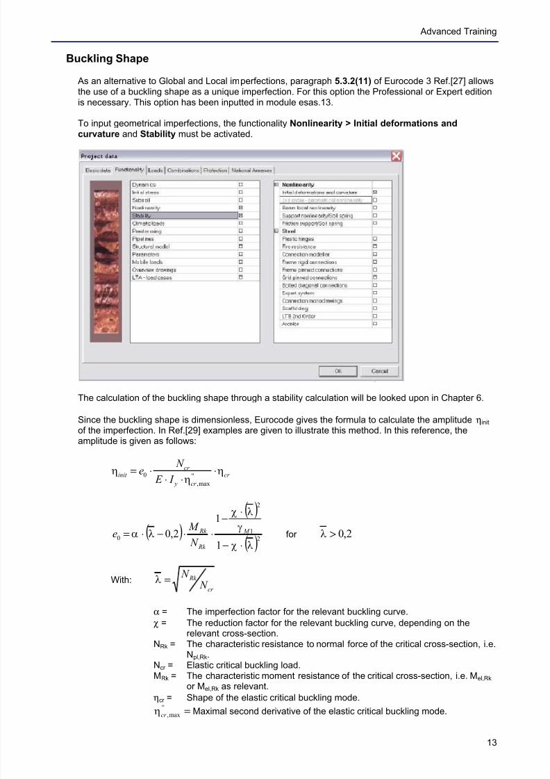
As an alternative to Global and Local imperfections, paragraph 5.3.2(11) of Eurocode 3 Ref.[27] allowsthe use of a buckling shape as a unique imperfection. For this option the Professional or Expert editionis necessary. This option has been inputted in module esas.13.
To input geometrical imperfections, the functionality Nonlinearity > Initial deformations and
curvature and Stability must be activated.
The calculation of the buckling shape through a stability calculation will be looked upon in Chapter 6.
Since the buckling shape is dimensionless, Eurocode gives the formula to calculate the amplitude ηinit of the imperfection. In Ref.[29] examples are given to illustrate this method. In this reference, theamplitude is given as follows:
cr
cr y
cr init
I E
N e η
ηη ⋅
⋅⋅⋅=
''
max,
0
( )
( )
( )2
1
2
0
1
1
2,0
λχ
γ
λχ
λα
⋅−
⋅−
⋅⋅−⋅= M
Rk
Rk
N
M e for 2,0>λ
With:cr
Rk
N N
=λ
α = The imperfection factor for the relevant buckling curve.
χ = The reduction factor for the relevant buckling curve, depending on therelevant cross-section.
NRk = The characteristic resistance to normal force of the critical cross-section, i.e.Npl,Rk.
Ncr = Elastic critical buckling load.MRk = The characteristic moment resistance of the critical cross-section, i.e. Mel,Rk
or Mel,Rk as relevant.
ηcr = Shape of the elastic critical buckling mode.
=''
max,cr η Maximal second derivative of the elastic critical buckling mode.
7/18/2019 Nonlinear and Stability 2013
http://slidepdf.com/reader/full/nonlinear-and-stability-2013 18/106
Non linear and Stability
14
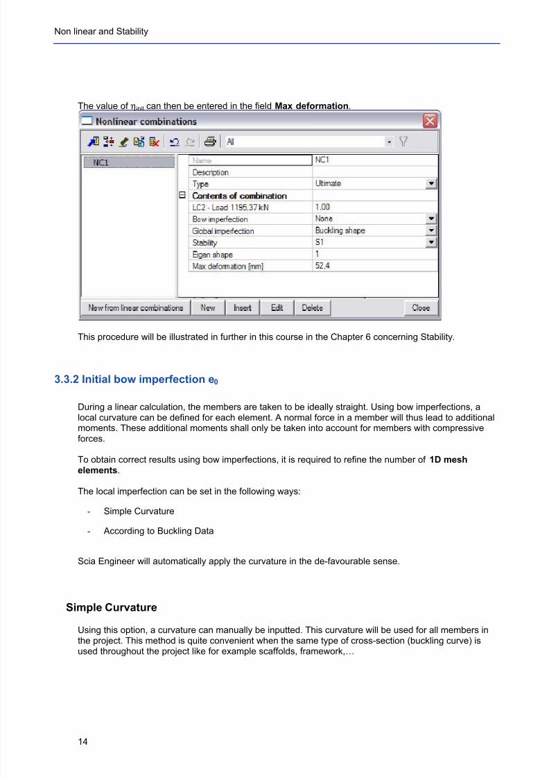
The value of ηinit can then be entered in the field Max deformation.
This procedure will be illustrated in further in this course in the Chapter 6 concerning Stability.
3.3.2 Initial bow imperfection e0
During a linear calculation, the members are taken to be ideally straight. Using bow imperfections, alocal curvature can be defined for each element. A normal force in a member will thus lead to additionalmoments. These additional moments shall only be taken into account for members with compressiveforces.
To obtain correct results using bow imperfections, it is required to refine the number of 1D meshelements.
The local imperfection can be set in the following ways:
- Simple Curvature
- According to Buckling Data
Scia Engineer will automatically apply the curvature in the de-favourable sense.
Simple Curvature
Using this option, a curvature can manually be inputted. This curvature will be used for all members inthe project. This method is quite convenient when the same type of cross-section (buckling curve) isused throughout the project like for example scaffolds, framework,…
7/18/2019 Nonlinear and Stability 2013
http://slidepdf.com/reader/full/nonlinear-and-stability-2013 19/106
Advanced Training
15
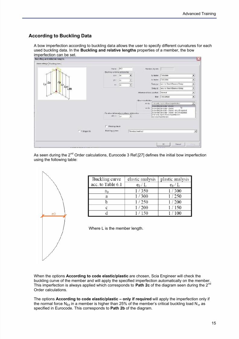
According to Buckling Data
A bow imperfection according to buckling data allows the user to specify different curvatures for eachused buckling data. In the Buckling and relative lengths properties of a member, the bowimperfection can be set.
As seen during the 2nd
Order calculations, Eurocode 3 Ref.[27] defines the initial bow imperfectionusing the following table:
Where L is the member length.
When the options According to code elastic/plastic are chosen, Scia Engineer will check thebuckling curve of the member and will apply the specified imperfection automatically on the member.This imperfection is always applied which corresponds to Path 2c of the diagram seen during the 2
nd
Order calculations.
The options According to code elastic/plastic – only if required will apply the imperfection only if
the normal force NEd in a member is higher than 25% of the member’s critical buckling load Ncr asspecified in Eurocode. This corresponds to Path 2b of the diagram.
7/18/2019 Nonlinear and Stability 2013
http://slidepdf.com/reader/full/nonlinear-and-stability-2013 20/106
7/18/2019 Nonlinear and Stability 2013
http://slidepdf.com/reader/full/nonlinear-and-stability-2013 21/106
Advanced Training
17
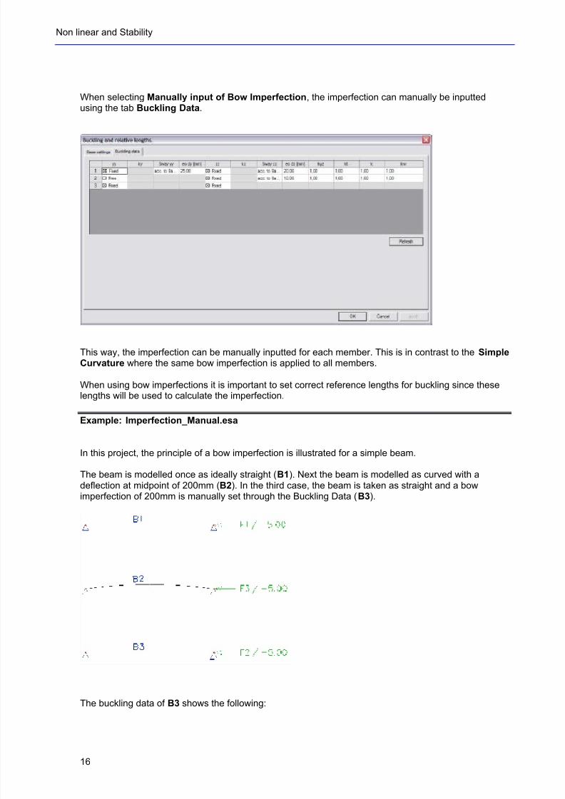
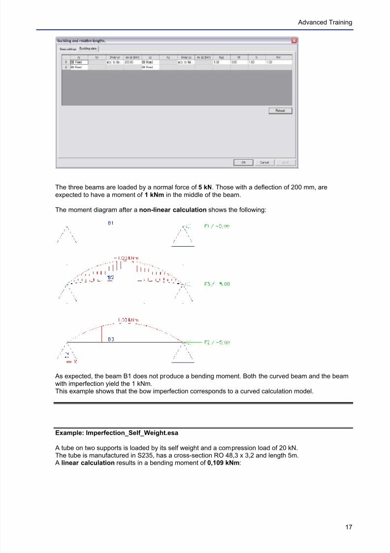
The three beams are loaded by a normal force of 5 kN. Those with a deflection of 200 mm, are
expected to have a moment of 1 kNm in the middle of the beam.
The moment diagram after a non-linear calculation shows the following:
As expected, the beam B1 does not produce a bending moment. Both the curved beam and the beamwith imperfection yield the 1 kNm.This example shows that the bow imperfection corresponds to a curved calculation model.
Example: Imperfection_Self_Weight.esa
A tube on two supports is loaded by its self weight and a compression load of 20 kN.The tube is manufactured in S235, has a cross-section RO 48,3 x 3,2 and length 5m.
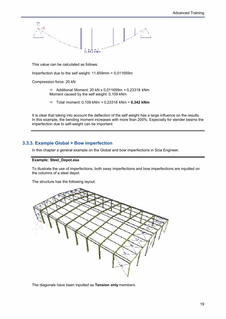
A linear calculation results in a bending moment of 0,109 kNm:
7/18/2019 Nonlinear and Stability 2013
http://slidepdf.com/reader/full/nonlinear-and-stability-2013 22/106
7/18/2019 Nonlinear and Stability 2013
http://slidepdf.com/reader/full/nonlinear-and-stability-2013 23/106
Advanced Training
19
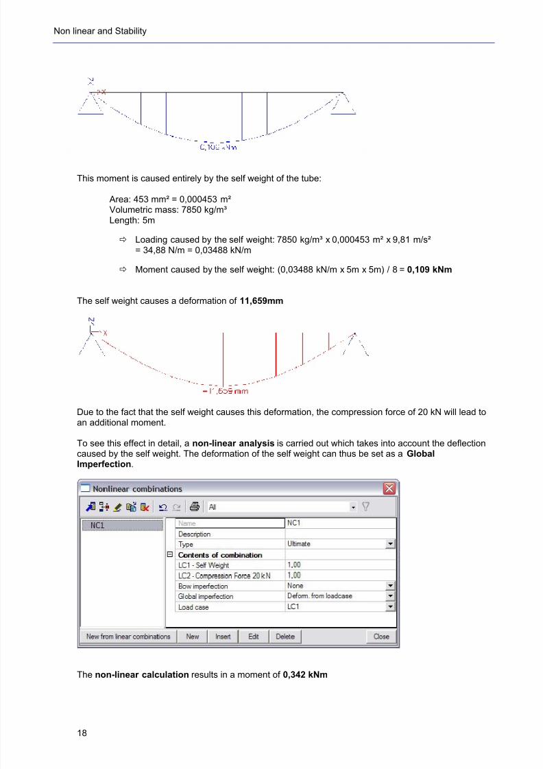
This value can be calculated as follows:
Imperfection due to the self weight: 11,659mm = 0,011659m
Compression force: 20 kN
ð Additional Moment: 20 kN x 0,011659m = 0,23318 kNmMoment caused by the self weight: 0,109 kNm
ð Total moment: 0,109 kNm + 0,23318 kNm = 0,342 kNm
It is clear that taking into account the deflection of the self weight has a large influence on the results.In this example, the bending moment increases with more than 200%. Especially for slender beams theimperfection due to self-weight can be important.
3.3.3. Example Global + Bow imperfection
In this chapter a general example on the Global and bow imperfections in Scia Engineer.
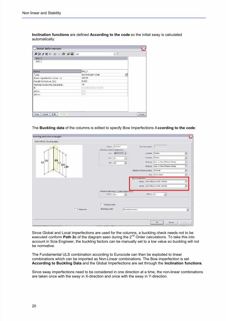
Example: Steel_Depot.esa
To illustrate the use of imperfections, both sway imperfections and bow imperfections are inputted onthe columns of a steel depot.
The structure has the following layout:
The diagonals have been inputted as Tension only members.
7/18/2019 Nonlinear and Stability 2013
http://slidepdf.com/reader/full/nonlinear-and-stability-2013 24/106
Non linear and Stability
20
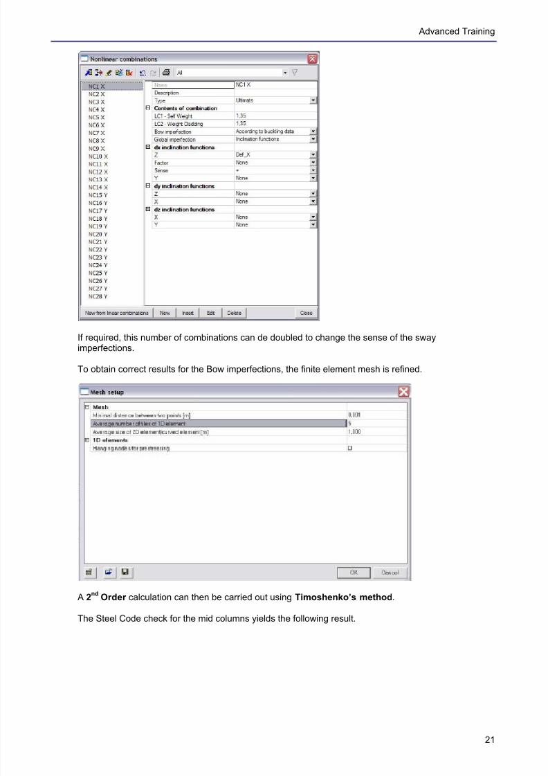
Inclination functions are defined According to the code so the initial sway is calculatedautomatically:
The Buckling data of the columns is edited to specify Bow Imperfections According to the code:
Since Global and Local imperfections are used for the columns, a buckling check needs not to beexecuted conform Path 2c of the diagram seen during the 2
nd Order calculations. To take this into
account in Scia Engineer, the buckling factors can be manually set to a low value so buckling will notbe normative.
The Fundamental ULS combination according to Eurocode can then be exploded to linearcombinations which can be imported as Non-Linear combinations. The Bow imperfection is setAccording to Buckling Data and the Global Imperfections are set through the Inclination functions.
Since sway imperfections need to be considered in one direction at a time, the non-linear combinationsare taken once with the sway in X-direction and once with the sway in Y-direction.
7/18/2019 Nonlinear and Stability 2013
http://slidepdf.com/reader/full/nonlinear-and-stability-2013 25/106
Advanced Training
21
If required, this number of combinations can de doubled to change the sense of the swayimperfections.
To obtain correct results for the Bow imperfections, the finite element mesh is refined.
A 2nd
Order calculation can then be carried out using Timoshenko’s method.
The Steel Code check for the mid columns yields the following result.
7/18/2019 Nonlinear and Stability 2013
http://slidepdf.com/reader/full/nonlinear-and-stability-2013 26/106
Non linear and Stability
22
Since both global and local imperfections have been inputted, only the Section check and the LateralTorsional Buckling check are relevant. In this example, member B9 produces the largest check on the
compression and bending check.
3.4. The second order calculation
3.4.1. Timoshenko
The first method is the so called Timoshenko method (Th.II.O) which is based on the exactTimoshenko solution for members with known normal force. It is a 2
nd order theory with equilibrium on
the deformed structure which assumes small displacements, small rotations and small strains.
When the normal force in a member is smaller than the critical buckling load, this method is very solid.The axial force is assumed constant during the deformation. Therefore, the method is applicable whenthe normal forces (or membrane forces) do not alter substantially after the first iteration. This is truemainly for frames, buildings, etc. for which the method is the most effective option.
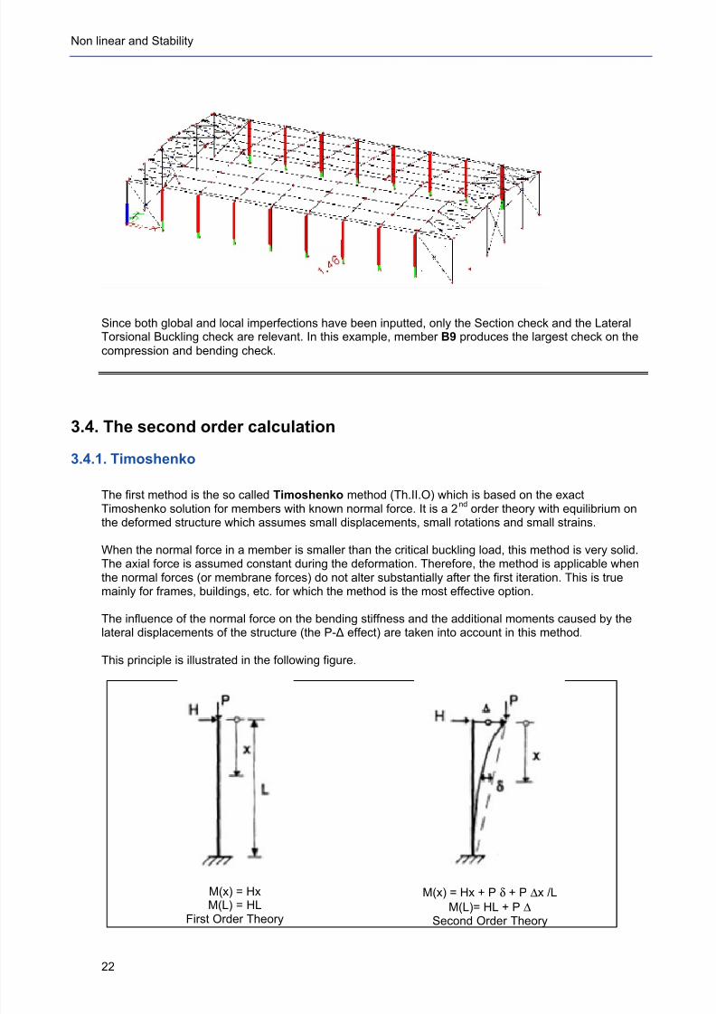
The influence of the normal force on the bending stiffness and the additional moments caused by thelateral displacements of the structure (the P- ! effect) are taken into account in this method.
This principle is illustrated in the following figure.
M(x) = HxM(L) = HL
First Order Theory
M(x) = Hx + P δ + P ∆x /LM(L)= HL + P ∆
Second Order Theory

7/18/2019 Nonlinear and Stability 2013
http://slidepdf.com/reader/full/nonlinear-and-stability-2013 27/106
7/18/2019 Nonlinear and Stability 2013
http://slidepdf.com/reader/full/nonlinear-and-stability-2013 28/106
Non linear and Stability
24
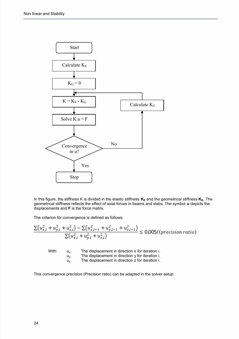
In this figure, the stiffness K is divided in the elastic stiffness KE and the geometrical stiffness KG. Thegeometrical stiffness reflects the effect of axial forces in beams and slabs. The symbol u depicts thedisplacements and F is the force matrix.
The criterion for convergence is defined as follows:
@ABC,DE + FG,HI + JK,LM N O @PQR,STUV + WX,YZ[\ + ]^,_`ab c@def,gh + ij,kl + mn,op q 7
0,005/ (
rstuvwxyz |}~•!)
With: ux,i The displacement in direction x for iteration i.uy,i The displacement in direction y for iteration i.uz,i The displacement in direction z for iteration i.
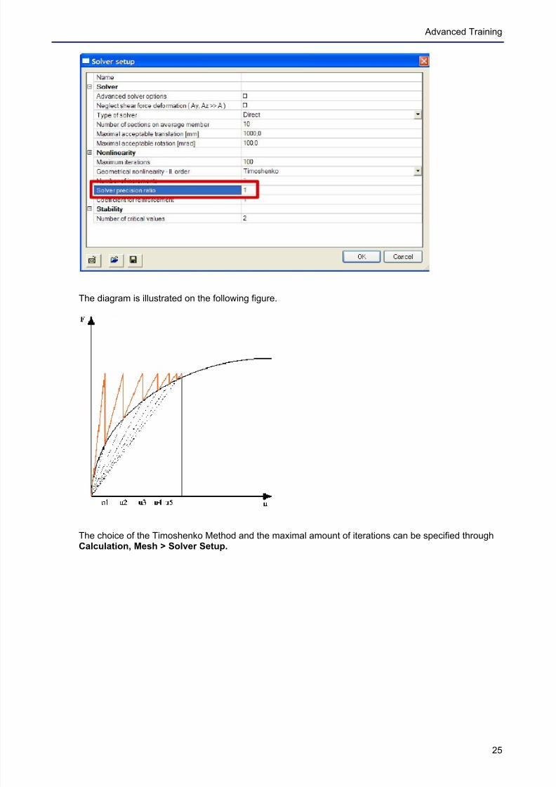
This convergence precision (Precision ratio) can be adapted in the solver setup:
Start
Stop
Calculate K E
K G = 0
K = K E - K G
Solve K.u = F
Convergence
in u?
Calculate K G
No
Yes
7/18/2019 Nonlinear and Stability 2013
http://slidepdf.com/reader/full/nonlinear-and-stability-2013 29/106
Advanced Training
25
The diagram is illustrated on the following figure.
The choice of the Timoshenko Method and the maximal amount of iterations can be specified throughCalculation, Mesh > Solver Setup.
7/18/2019 Nonlinear and Stability 2013
http://slidepdf.com/reader/full/nonlinear-and-stability-2013 30/106
Non linear and Stability
26
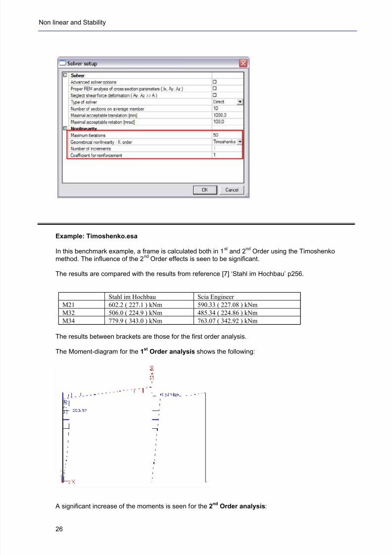
Example: Timoshenko.esa
In this benchmark example, a frame is calculated both in 1st and 2
nd Order using the Timoshenko
method. The influence of the 2nd
Order effects is seen to be significant.
The results are compared with the results from reference [7] ‘Stahl im Hochbau’ p256.
Stahl im Hochbau Scia Engineer
M21 602.2 ( 227.1 ) kNm 590.33 ( 227.08 ) kNm
M32 506.0 ( 224.9 ) kNm 485.34 ( 224.86 ) kNm
M34 779.9 ( 343.0 ) kNm 763.07 ( 342.92 ) kNm
The results between brackets are those for the first order analysis.
The Moment-diagram for the 1st
Order analysis shows the following:
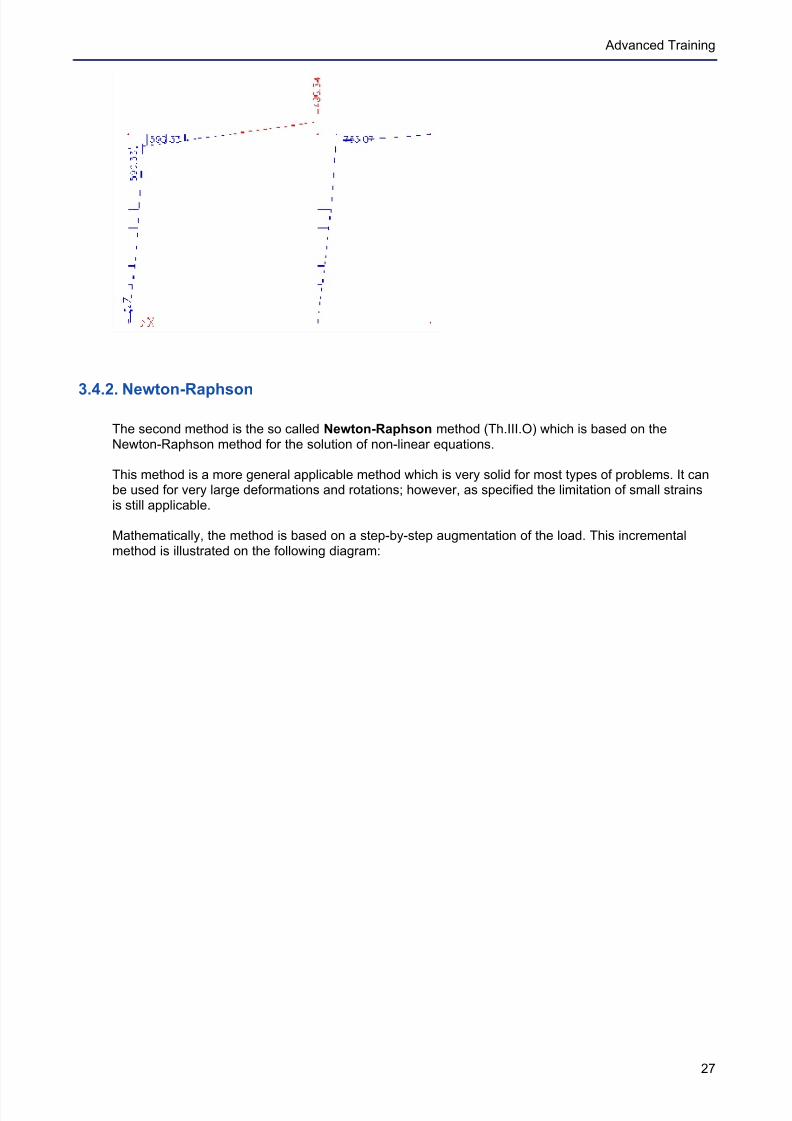
A significant increase of the moments is seen for the 2nd
Order analysis:
7/18/2019 Nonlinear and Stability 2013
http://slidepdf.com/reader/full/nonlinear-and-stability-2013 31/106
Advanced Training
27
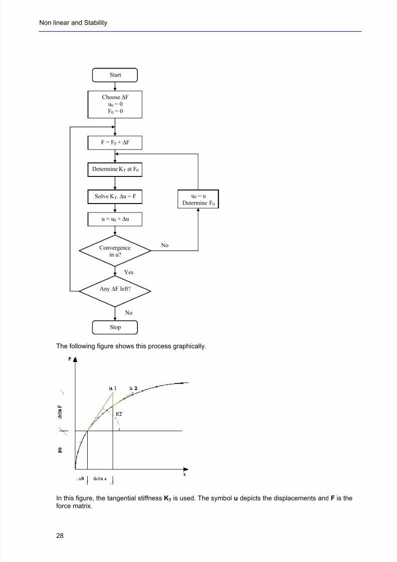
3.4.2. Newton-Raphson
The second method is the so called Newton-Raphson method (Th.III.O) which is based on theNewton-Raphson method for the solution of non-linear equations.
This method is a more general applicable method which is very solid for most types of problems. It canbe used for very large deformations and rotations; however, as specified the limitation of small strainsis still applicable.
Mathematically, the method is based on a step-by-step augmentation of the load. This incrementalmethod is illustrated on the following diagram:
7/18/2019 Nonlinear and Stability 2013
http://slidepdf.com/reader/full/nonlinear-and-stability-2013 32/106
7/18/2019 Nonlinear and Stability 2013
http://slidepdf.com/reader/full/nonlinear-and-stability-2013 33/106
Advanced Training
29
The original Newton-Raphson method changes the tangential stiffness in each iteration. There are alsoadapted procedures which keep the stiffness constant in certain zones during for example oneincrement. Scia Engineer uses the original method.
As a limitation, the rotation achieved in one increment should not exceed 5°.
The accuracy of the method can be increased through refinement of the finite element mesh and byincreasing the number of increments. By default, when the Newton-Raphson method is used, thenumber of 1D elements is set to 4 and the Number of increments is set to 5.
In some cases, a high number of increments may even solve problems that tend to a singular solutionwhich is typical for the analysis of post-critical states. However, in most cases, such a state ischaracterized by extreme deformations, which is not interesting for design purposes.
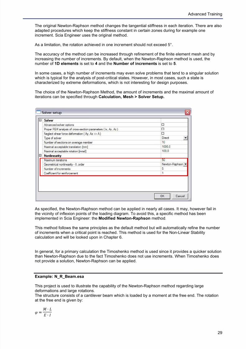
The choice of the Newton-Raphson Method, the amount of increments and the maximal amount ofiterations can be specified through Calculation, Mesh > Solver Setup.
As specified, the Newton-Raphson method can be applied in nearly all cases. It may, however fail inthe vicinity of inflexion points of the loading diagram. To avoid this, a specific method has beenimplemented in Scia Engineer: the Modified Newton-Raphson method.
This method follows the same principles as the default method but will automatically refine the numberof increments when a critical point is reached. This method is used for the Non-Linear Stabilitycalculation and will be looked upon in Chapter 6.
In general, for a primary calculation the Timoshenko method is used since it provides a quicker solutionthan Newton-Raphson due to the fact Timoshenko does not use increments. When Timoshenko doesnot provide a solution, Newton-Raphson can be applied.
Example: N_R_Beam.esa
This project is used to illustrate the capability of the Newton-Raphson method regarding largedeformations and large rotations.The structure consists of a cantilever beam which is loaded by a moment at the free end. The rotationat the free end is given by:
" = # + $% + &
7/18/2019 Nonlinear and Stability 2013
http://slidepdf.com/reader/full/nonlinear-and-stability-2013 34/106
Non linear and Stability
30
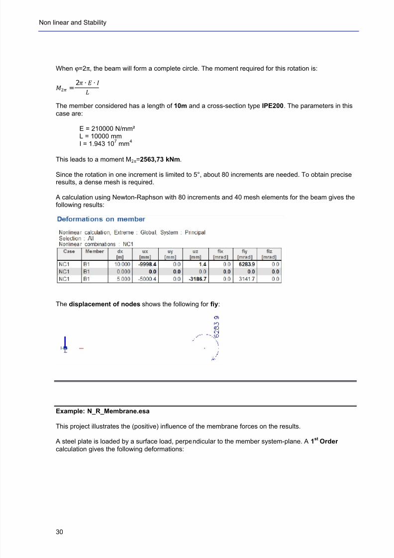
When ϕ=2π, the beam will form a complete circle. The moment required for this rotation is:
'() =
2* + + + ,-
The member considered has a length of 10m and a cross-section type IPE200. The parameters in this
case are:
E = 210000 N/mm²L = 10000 mmI = 1.943 10
7 mm
4
This leads to a moment M2π=2563,73 kNm.
Since the rotation in one increment is limited to 5°, about 80 increments are needed. To obtain preciseresults, a dense mesh is required.
A calculation using Newton-Raphson with 80 increments and 40 mesh elements for the beam gives thefollowing results:
The displacement of nodes shows the following for fiy:
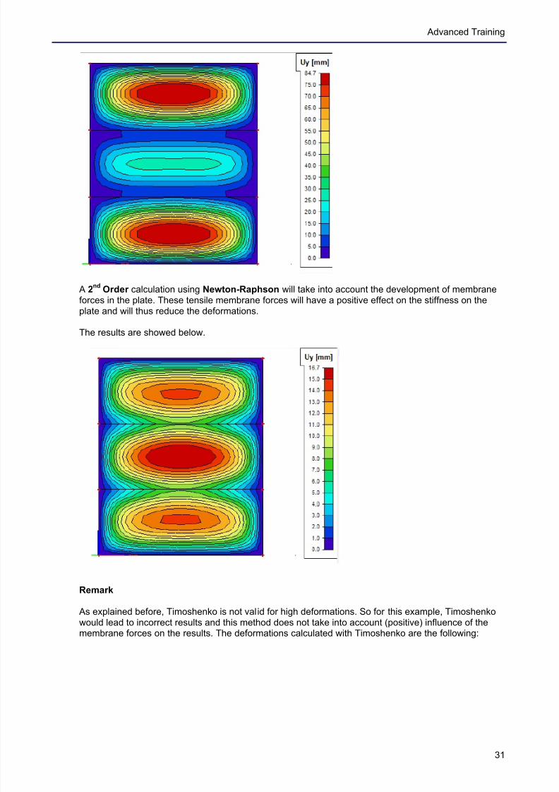
Example: N_R_Membrane.esa
This project illustrates the (positive) influence of the membrane forces on the results.
A steel plate is loaded by a surface load, perpendicular to the member system-plane. A 1st
Order
calculation gives the following deformations:
7/18/2019 Nonlinear and Stability 2013
http://slidepdf.com/reader/full/nonlinear-and-stability-2013 35/106
Advanced Training
31
A 2nd
Order calculation using Newton-Raphson will take into account the development of membraneforces in the plate. These tensile membrane forces will have a positive effect on the stiffness on theplate and will thus reduce the deformations.
The results are showed below.
Remark
As explained before, Timoshenko is not valid for high deformations. So for this example, Timoshenkowould lead to incorrect results and this method does not take into account (positive) influence of themembrane forces on the results. The deformations calculated with Timoshenko are the following:
7/18/2019 Nonlinear and Stability 2013
http://slidepdf.com/reader/full/nonlinear-and-stability-2013 36/106
Non linear and Stability
32
7/18/2019 Nonlinear and Stability 2013
http://slidepdf.com/reader/full/nonlinear-and-stability-2013 37/106
Advanced Training
33
4. Physical Non-Linearity
When the stresses are dependent on the strains in a non linear way, the non linearity is called aphysical non linearity.
In Scia Engineer, the following types of physical non linearities have been implemented:
- Plastic Hinges for Steel Structures
- Physical Non-Linear analysis for Concrete Structures
4.1 Plastic Hinges for Steel Structures
When a normal linear calculation is performed and limit stress is achieved in any part of the structure,the dimension of critical elements must be increased. If however, plastic hinges are taken into account,the achievement of limit stress causes the formation of plastic hinges at appropriate joints and thecalculation can continue with another iteration step. The stress is redistributed to other parts of thestructure and better utilization of overall load bearing capacity of the structure is obtained.
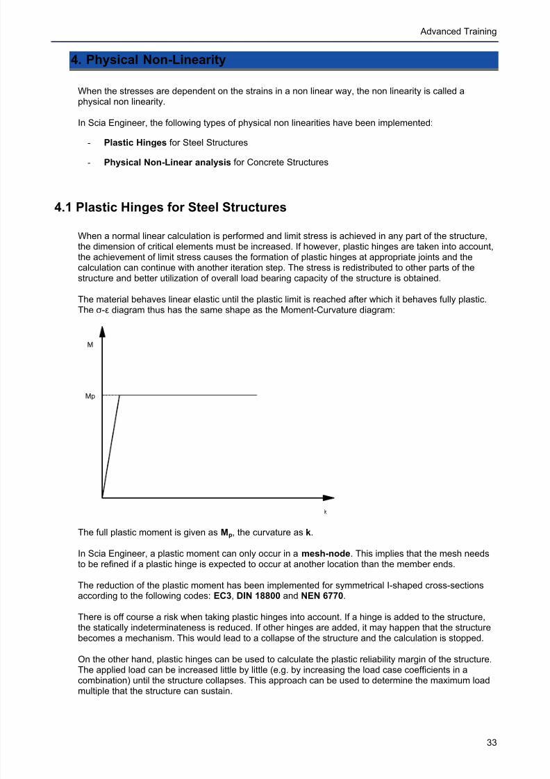
The material behaves linear elastic until the plastic limit is reached after which it behaves fully plastic.The "-# diagram thus has the same shape as the Moment-Curvature diagram:
M
k
Mp
The full plastic moment is given as Mp, the curvature as k.
In Scia Engineer, a plastic moment can only occur in a mesh-node. This implies that the mesh needsto be refined if a plastic hinge is expected to occur at another location than the member ends.
The reduction of the plastic moment has been implemented for symmetrical I-shaped cross-sectionsaccording to the following codes: EC3, DIN 18800 and NEN 6770.
There is off course a risk when taking plastic hinges into account. If a hinge is added to the structure,the statically indeterminateness is reduced. If other hinges are added, it may happen that the structurebecomes a mechanism. This would lead to a collapse of the structure and the calculation is stopped.
On the other hand, plastic hinges can be used to calculate the plastic reliability margin of the structure.The applied load can be increased little by little (e.g. by increasing the load case coefficients in a
combination) until the structure collapses. This approach can be used to determine the maximum loadmultiple that the structure can sustain.
7/18/2019 Nonlinear and Stability 2013
http://slidepdf.com/reader/full/nonlinear-and-stability-2013 38/106
Non linear and Stability
34
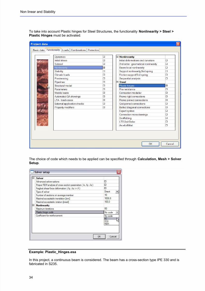
To take into account Plastic hinges for Steel Structures, the functionality Nonlinearity > Steel >Plastic Hinges must be activated.
The choice of code which needs to be applied can be specified through Calculation, Mesh > SolverSetup.
Example: Plastic_Hinges.esa
In this project, a continuous beam is considered. The beam has a cross-section type IPE 330 and isfabricated in S235.
7/18/2019 Nonlinear and Stability 2013
http://slidepdf.com/reader/full/nonlinear-and-stability-2013 39/106
Advanced Training
35
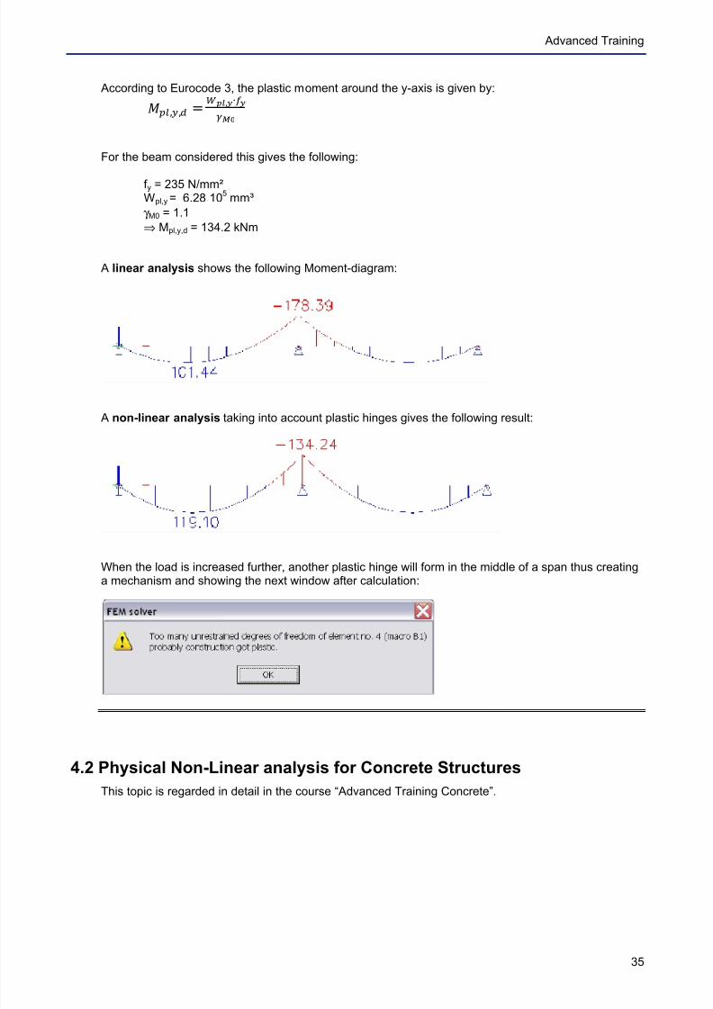
According to Eurocode 3, the plastic moment around the y-axis is given by:./0,1,2 =345,6+789:;
For the beam considered this gives the following:
f y = 235 N/mm²Wpl,y = 6.28 10
5 mm³
γ M0 = 1.1
⇒ Mpl,y,d = 134.2 kNm
A linear analysis shows the following Moment-diagram:
A non-linear analysis taking into account plastic hinges gives the following result:
When the load is increased further, another plastic hinge will form in the middle of a span thus creatinga mechanism and showing the next window after calculation:
4.2 Physical Non-Linear analysis for Concrete Structures
This topic is regarded in detail in the course “Advanced Training Concrete”.
7/18/2019 Nonlinear and Stability 2013
http://slidepdf.com/reader/full/nonlinear-and-stability-2013 40/106
Non linear and Stability
36
5. Local Non-Linearity
The local non linearities can be defined for 1D members, connections between 1D members, 2Dmembers and supports.
The following types have been implemented in Scia Engineer:
- Beam local nonlinearity
- Beam local nonlinearity including initial Stress
- Non-linear member connections
- Support nonlinearity
- Pressure only elements
- 2D Membrane Elements
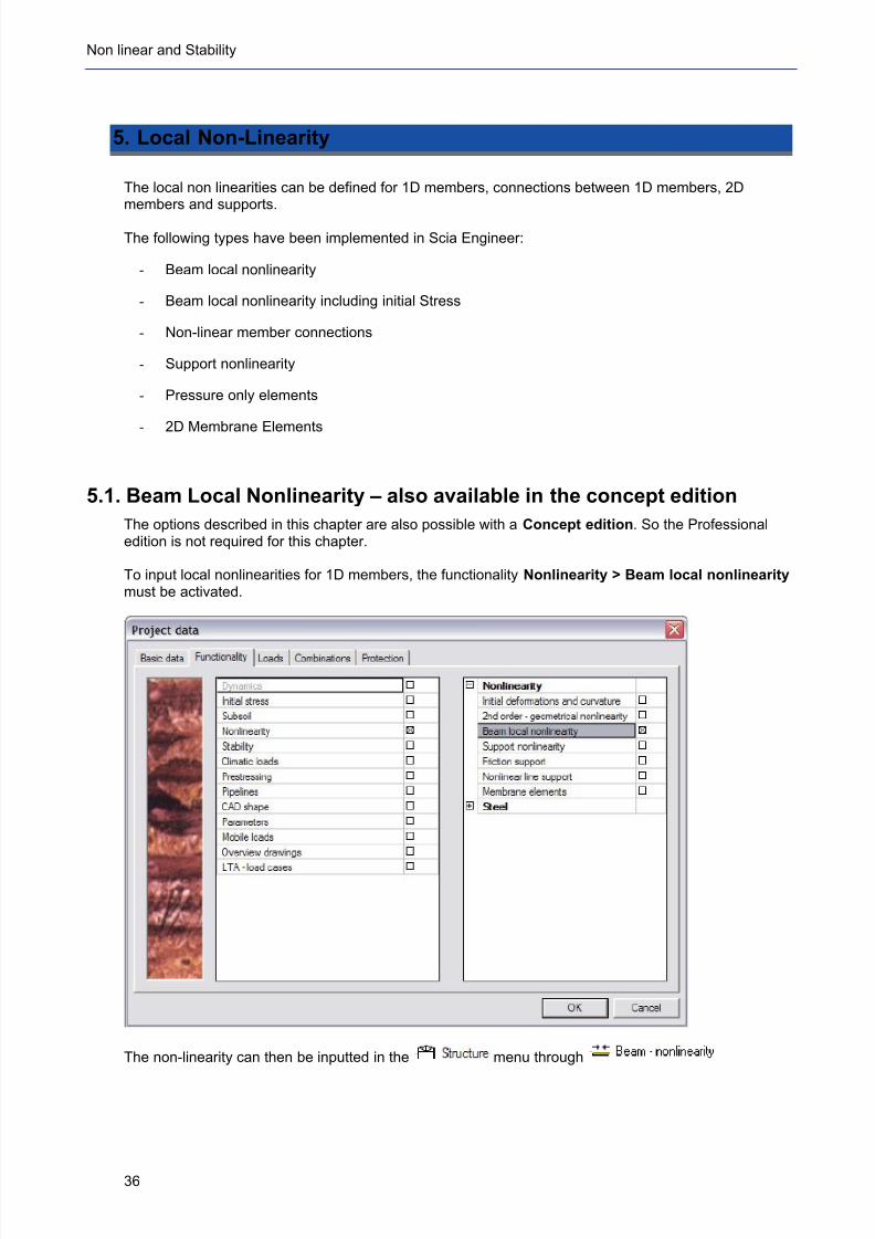
5.1. Beam Local Nonlinearity – also available in the concept edition
The options described in this chapter are also possible with a Concept edition. So the Professionaledition is not required for this chapter.
To input local nonlinearities for 1D members, the functionality Nonlinearity > Beam local nonlinearity must be activated.
The non-linearity can then be inputted in the menu through
7/18/2019 Nonlinear and Stability 2013
http://slidepdf.com/reader/full/nonlinear-and-stability-2013 41/106
Advanced Training
37
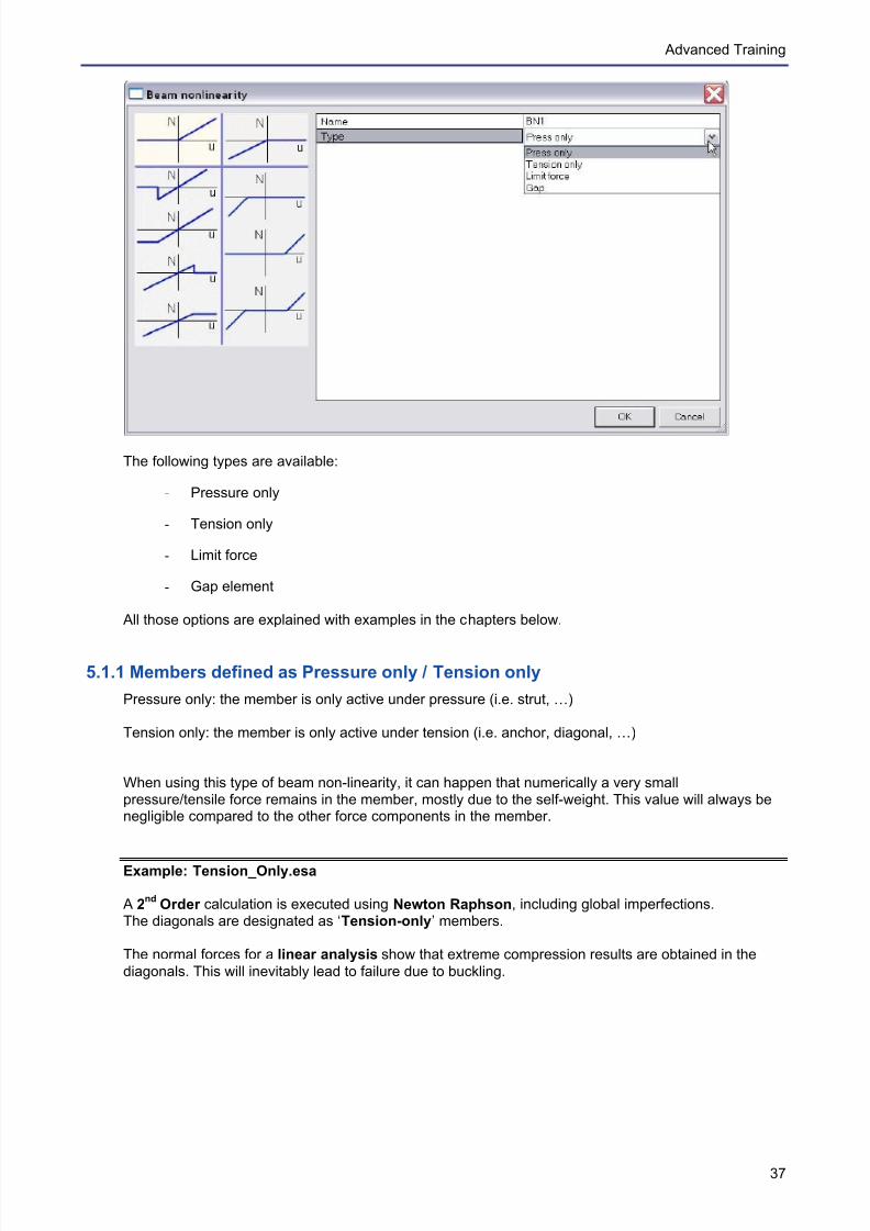
The following types are available:
- Pressure only
- Tension only
- Limit force
- Gap element
All those options are explained with examples in the chapters below.
5.1.1 Members defined as Pressure only / Tension only
Pressure only: the member is only active under pressure (i.e. strut, …)
Tension only: the member is only active under tension (i.e. anchor, diagonal, …)
When using this type of beam non-linearity, it can happen that numerically a very smallpressure/tensile force remains in the member, mostly due to the self-weight. This value will always benegligible compared to the other force components in the member.
Example: Tension_Only.esa
A 2nd
Order calculation is executed using Newton Raphson, including global imperfections.The diagonals are designated as ‘Tension-only’ members.
The normal forces for a linear analysis show that extreme compression results are obtained in the
diagonals. This will inevitably lead to failure due to buckling.
7/18/2019 Nonlinear and Stability 2013
http://slidepdf.com/reader/full/nonlinear-and-stability-2013 42/106
Non linear and Stability
38
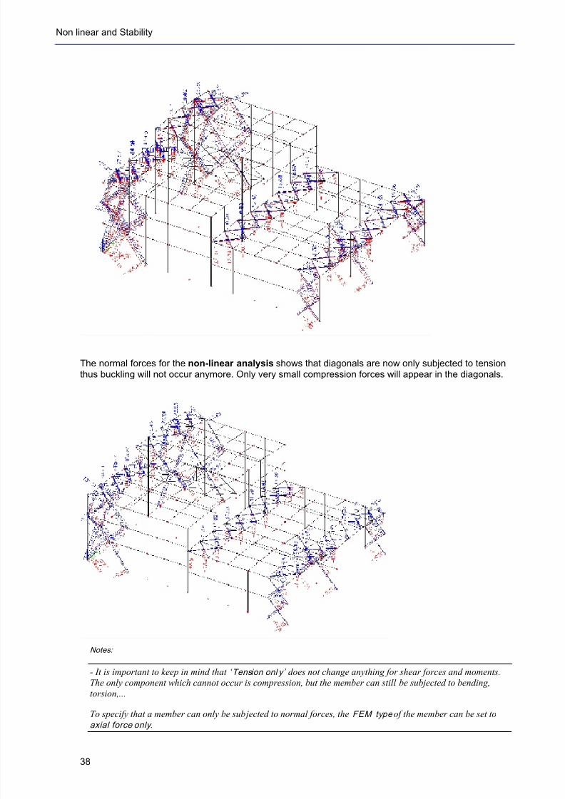
The normal forces for the non-linear analysis shows that diagonals are now only subjected to tensionthus buckling will not occur anymore. Only very small compression forces will appear in the diagonals.
Notes:
- It is important to keep in mind that ‘ Tension onl y ’ does not change anything for shear forces and moments.
The only component which cannot occur is compression, but the member can still be subjected to bending,
torsion,...
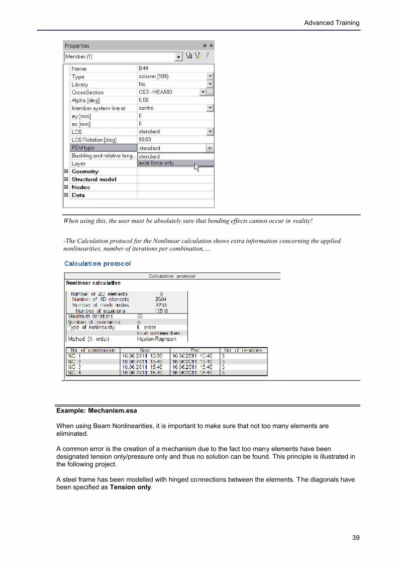
To specify that a member can only be subjected to normal forces, the FEM type of the member can be set to
axial force only .
7/18/2019 Nonlinear and Stability 2013
http://slidepdf.com/reader/full/nonlinear-and-stability-2013 43/106
Advanced Training
39
When using this, the user must be absolutely sure that bending effects cannot occur in reality!
-The Calculation protocol for the Nonlinear calculation shows extra information concerning the applied
nonlinearities, number of iterations per combination,…
Example: Mechanism.esa
When using Beam Nonlinearities, it is important to make sure that not too many elements areeliminated.
A common error is the creation of a mechanism due to the fact too many elements have beendesignated tension only/pressure only and thus no solution can be found. This principle is illustrated inthe following project.
A steel frame has been modelled with hinged connections between the elements. The diagonals havebeen specified as Tension only.
7/18/2019 Nonlinear and Stability 2013
http://slidepdf.com/reader/full/nonlinear-and-stability-2013 44/106
Non linear and Stability
40
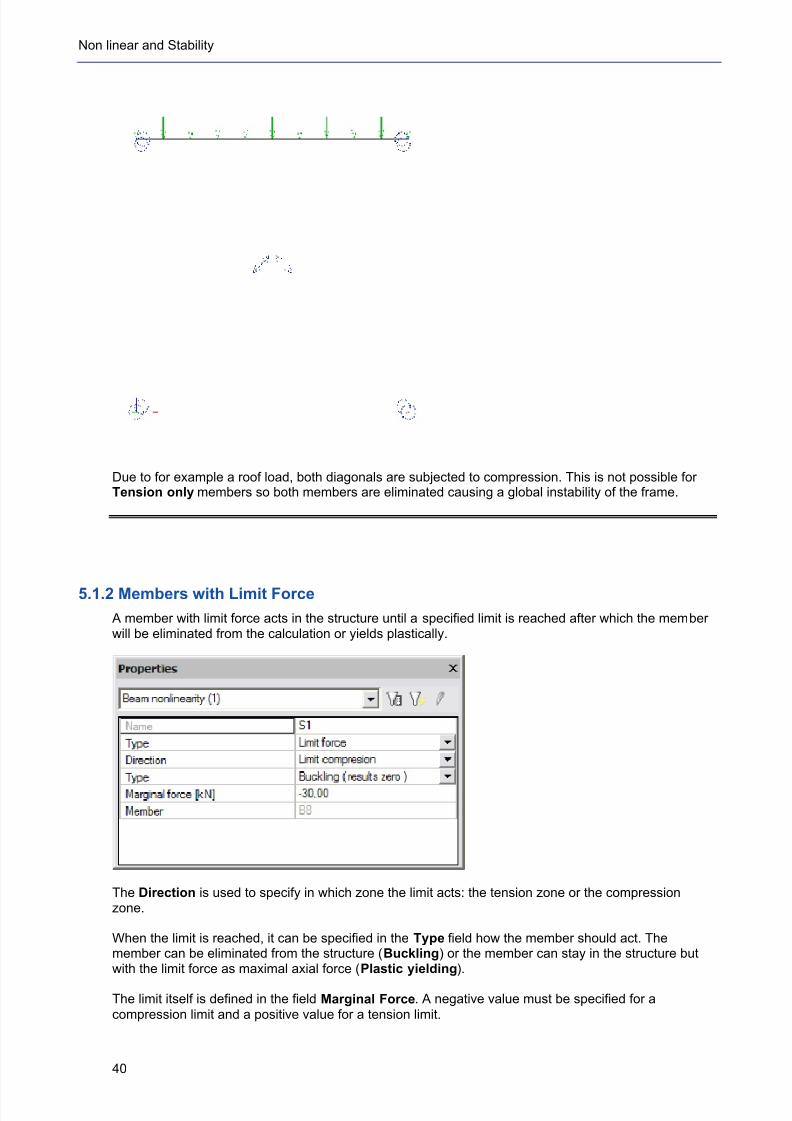
Due to for example a roof load, both diagonals are subjected to compression. This is not possible forTension only members so both members are eliminated causing a global instability of the frame.
5.1.2 Members with Limit Force
A member with limit force acts in the structure until a specified limit is reached after which the memberwill be eliminated from the calculation or yields plastically.
The Direction is used to specify in which zone the limit acts: the tension zone or the compressionzone.
When the limit is reached, it can be specified in the Type field how the member should act. Themember can be eliminated from the structure (Buckling) or the member can stay in the structure butwith the limit force as maximal axial force (Plastic yielding).
The limit itself is defined in the field Marginal Force. A negative value must be specified for a
compression limit and a positive value for a tension limit.
7/18/2019 Nonlinear and Stability 2013
http://slidepdf.com/reader/full/nonlinear-and-stability-2013 45/106
Advanced Training
41
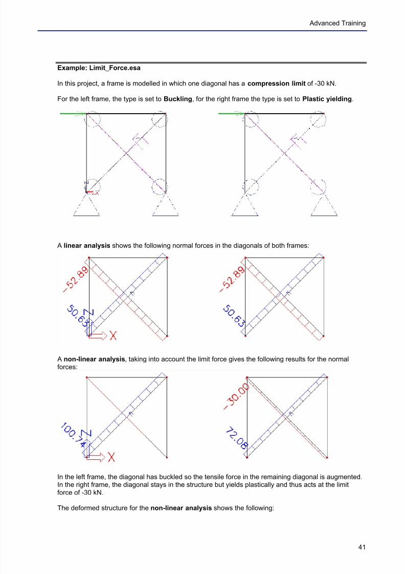
Example: Limit_Force.esa
In this project, a frame is modelled in which one diagonal has a compression limit of -30 kN.
For the left frame, the type is set to Buckling, for the right frame the type is set to Plastic yielding.
A linear analysis shows the following normal forces in the diagonals of both frames:
A non-linear analysis, taking into account the limit force gives the following results for the normalforces:
In the left frame, the diagonal has buckled so the tensile force in the remaining diagonal is augmented.In the right frame, the diagonal stays in the structure but yields plastically and thus acts at the limitforce of -30 kN.
The deformed structure for the non-linear analysis shows the following:
7/18/2019 Nonlinear and Stability 2013
http://slidepdf.com/reader/full/nonlinear-and-stability-2013 46/106
Non linear and Stability
42
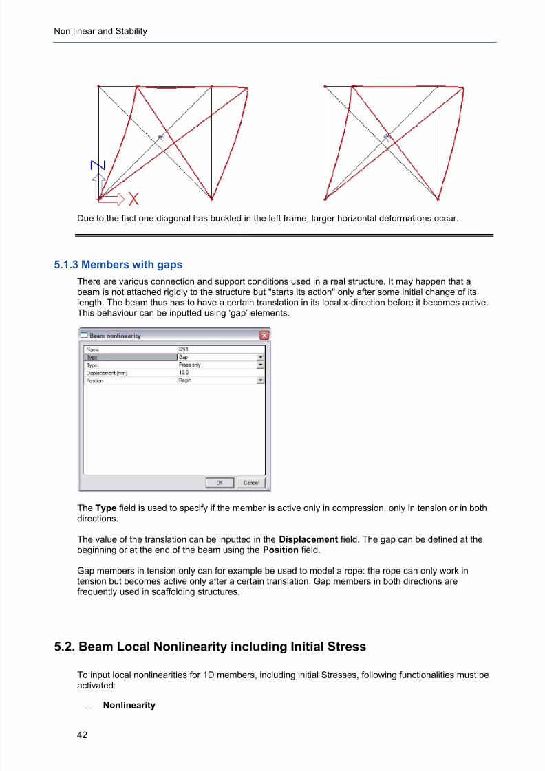
Due to the fact one diagonal has buckled in the left frame, larger horizontal deformations occur.
5.1.3 Members with gapsThere are various connection and support conditions used in a real structure. It may happen that abeam is not attached rigidly to the structure but "starts its action" only after some initial change of itslength. The beam thus has to have a certain translation in its local x-direction before it becomes active.This behaviour can be inputted using ‘gap’ elements.
The Type field is used to specify if the member is active only in compression, only in tension or in bothdirections.
The value of the translation can be inputted in the Displacement field. The gap can be defined at thebeginning or at the end of the beam using the Position field.
Gap members in tension only can for example be used to model a rope: the rope can only work intension but becomes active only after a certain translation. Gap members in both directions arefrequently used in scaffolding structures.
5.2. Beam Local Nonlinearity including Initial Stress
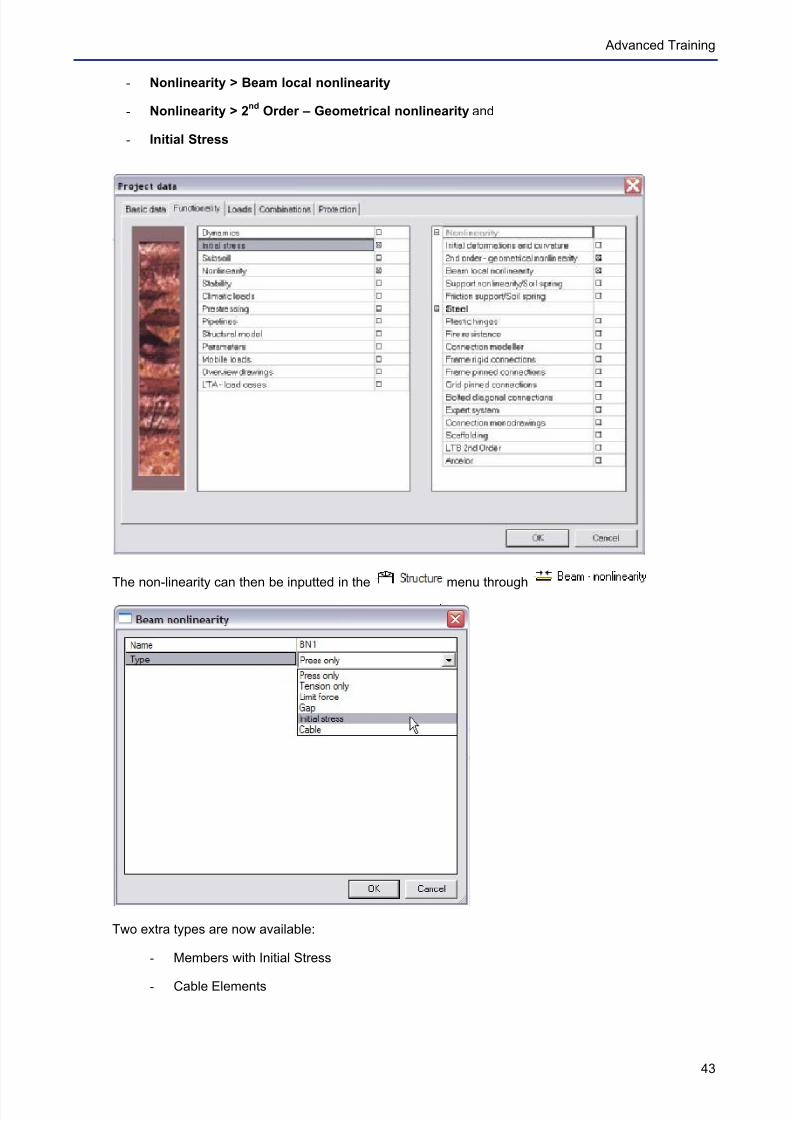
To input local nonlinearities for 1D members, including initial Stresses, following functionalities must beactivated:
- Nonlinearity
7/18/2019 Nonlinear and Stability 2013
http://slidepdf.com/reader/full/nonlinear-and-stability-2013 47/106
Advanced Training
43
- Nonlinearity > Beam local nonlinearity
- Nonlinearity > 2nd
Order – Geometrical nonlinearity and
- Initial Stress
The non-linearity can then be inputted in the menu through
Two extra types are now available:
- Members with Initial Stress
- Cable Elements

7/18/2019 Nonlinear and Stability 2013
http://slidepdf.com/reader/full/nonlinear-and-stability-2013 48/106
Non linear and Stability
44
5.2.1 Members with Initial Stress
Tensile forces in elements augment the stiffness of the structure. Compression forces reduce thestiffness.
Initial Stress is regarded as follows:
- The element in question is taken from the structure.
- The initial Stress is put on the element through the defined axial force.
- The element is put back into the structure.It is clear that, when the element is inserted into the structure, the initial stress will partly be given toother members thus the inputted force will not stay entirely in the member in question.
Notes:
- A positive axial force signifies a tensile force; a negative axial force signifies a compression force.
- Initial Stress is mostly used in conjunction with a 2nd
Order analysis.
- Initial Stress is the only local non-linearity taken into account in a Linear Stability Calculation. This type of
calculation will be regarded in Chapter 6 .
To take the inputted Initial Stresses into account for the calculation, the options Initial Stress andInitial Stress as input must be activated through Calculation, Mesh > Solver Setup.
Example: Initial_Stress.esa
In this project, a simple frame is modelled. The diagonal has a RD30 section and is given an InitialStress by means of a tensile force of 500 kN.
7/18/2019 Nonlinear and Stability 2013
http://slidepdf.com/reader/full/nonlinear-and-stability-2013 49/106
Advanced Training
45
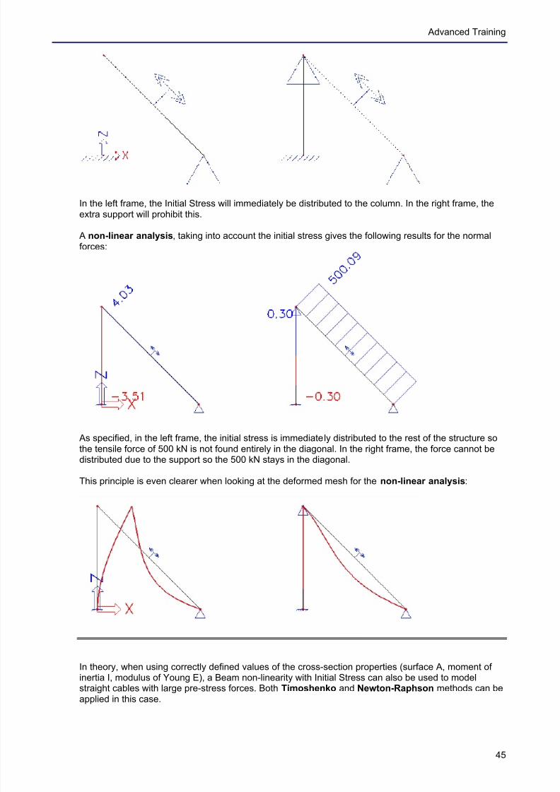
In the left frame, the Initial Stress will immediately be distributed to the column. In the right frame, theextra support will prohibit this.
A non-linear analysis, taking into account the initial stress gives the following results for the normalforces:
As specified, in the left frame, the initial stress is immediately distributed to the rest of the structure sothe tensile force of 500 kN is not found entirely in the diagonal. In the right frame, the force cannot bedistributed due to the support so the 500 kN stays in the diagonal.
This principle is even clearer when looking at the deformed mesh for the non-linear analysis:
In theory, when using correctly defined values of the cross-section properties (surface A, moment ofinertia I, modulus of Young E), a Beam non-linearity with Initial Stress can also be used to modelstraight cables with large pre-stress forces. Both Timoshenko and Newton-Raphson methods can beapplied in this case.
7/18/2019 Nonlinear and Stability 2013
http://slidepdf.com/reader/full/nonlinear-and-stability-2013 50/106
Non linear and Stability
46
In general however, for cables the use of the specific Cable element is advised in conjunction with theNewton-Raphson method.
5.2.2 Cable Elements – Not available in the Professional edition
This options needs module esas.12 and this module is included in the expert edition.
A Cable element is an element without bending stiffness (Iy and Iz ≅ 0). During the solving of theequations this is taken into account so no bending moment will occur in the element. Thedisplacements (in the intermediate nodes) have thus been calculated without bending stiffness.
A Cable element allows a precise analysis of cables. For slack cables, Scia Engineer allows thedefinition of the initial curved shape of the cable.
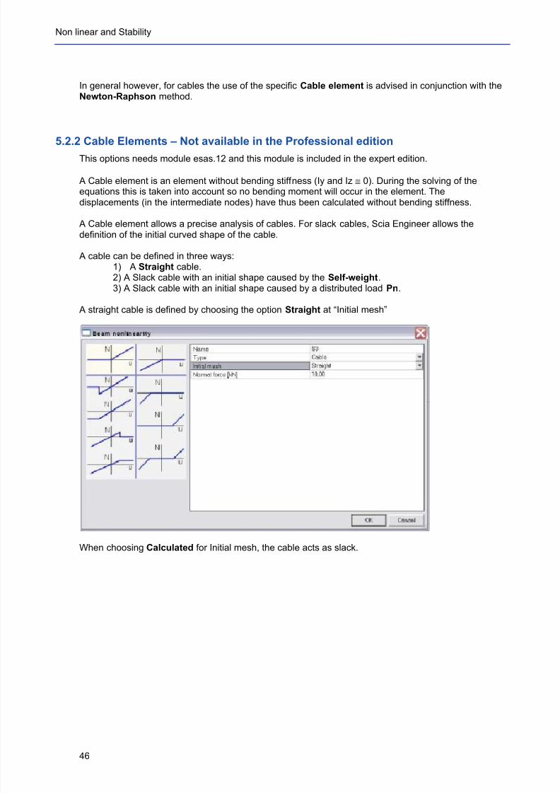
A cable can be defined in three ways:1) A Straight cable.
2) A Slack cable with an initial shape caused by the Self-weight.3) A Slack cable with an initial shape caused by a distributed load Pn.
A straight cable is defined by choosing the option Straight at “Initial mesh”
When choosing Calculated for Initial mesh, the cable acts as slack.
7/18/2019 Nonlinear and Stability 2013
http://slidepdf.com/reader/full/nonlinear-and-stability-2013 51/106
Advanced Training
47
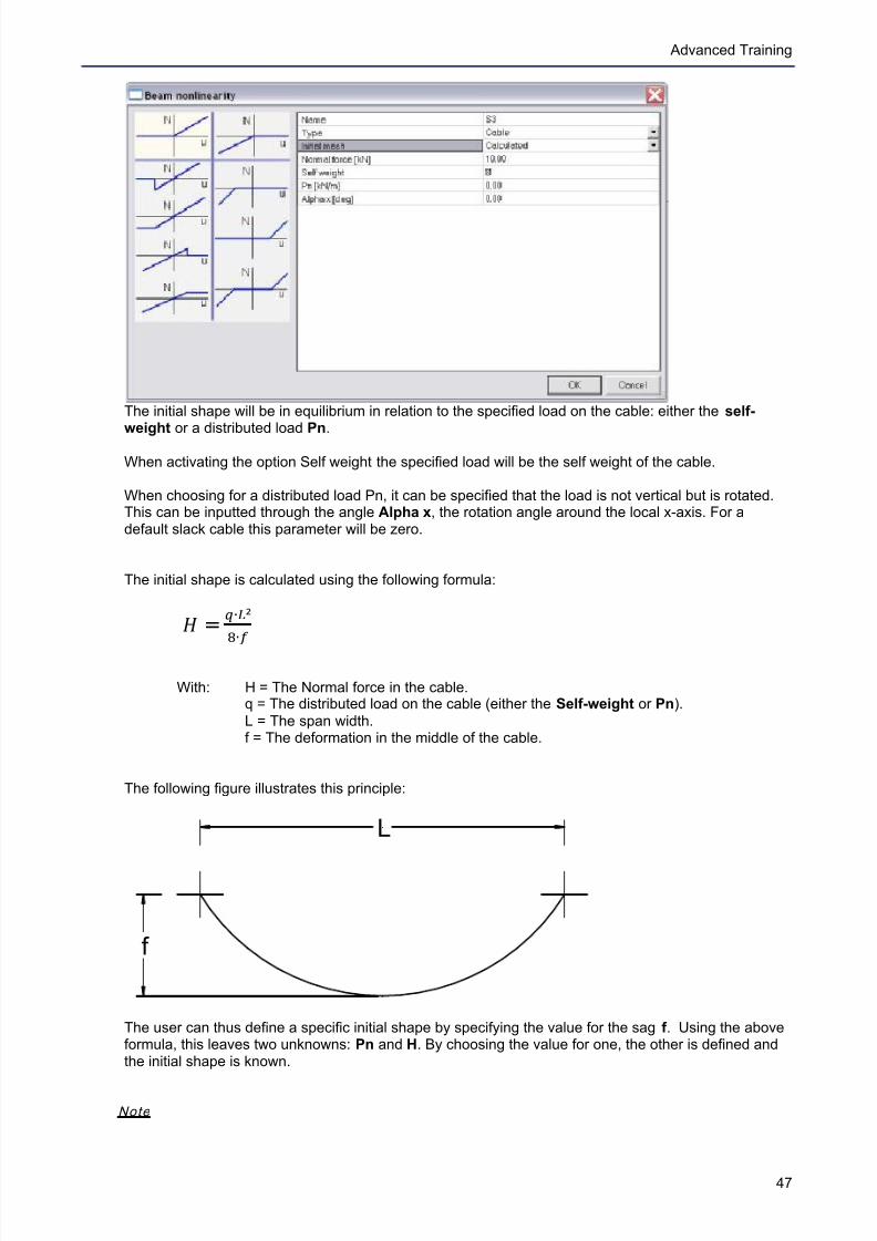
The initial shape will be in equilibrium in relation to the specified load on the cable: either the self-
weight or a distributed load Pn.
When activating the option Self weight the specified load will be the self weight of the cable.
When choosing for a distributed load Pn, it can be specified that the load is not vertical but is rotated.This can be inputted through the angle Alpha x, the rotation angle around the local x-axis. For adefault slack cable this parameter will be zero.
The initial shape is calculated using the following formula:
< =
=+>²
?+@
With: H = The Normal force in the cable.q = The distributed load on the cable (either the Self-weight or Pn).
L = The span width.f = The deformation in the middle of the cable.
The following figure illustrates this principle:
L
f
The user can thus define a specific initial shape by specifying the value for the sag f . Using the aboveformula, this leaves two unknowns: Pn and H. By choosing the value for one, the other is defined andthe initial shape is known.
Note
7/18/2019 Nonlinear and Stability 2013
http://slidepdf.com/reader/full/nonlinear-and-stability-2013 52/106
Non linear and Stability
48
- The input of the cable element only defines the initial shape. Afterwards the cable can beloaded by real loads.
- The calculations are executed on the deformed shape. This indicates that the eventualdeformation of a cable is calculated from the slack shape and not from the initial straight
shape.- The deformed mesh can be used to show the true deformation of the cable.
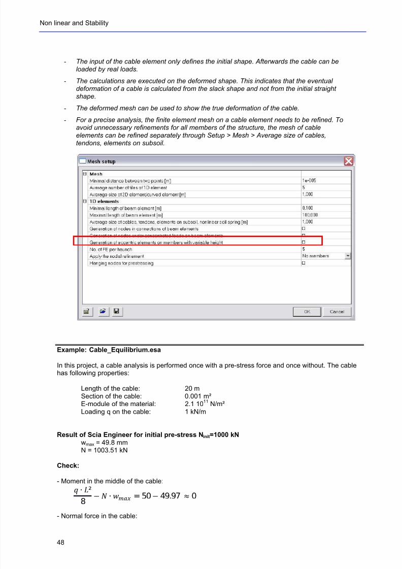
- For a precise analysis, the finite element mesh on a cable element needs to be refined. Toavoid unnecessary refinements for all members of the structure, the mesh of cableelements can be refined separately through Setup > Mesh > Average size of cables,tendons, elements on subsoil.
Example: Cable_Equilibrium.esa
In this project, a cable analysis is performed once with a pre-stress force and once without. The cablehas following properties:
Length of the cable: 20 m
Section of the cable: 0.001 m²E-module of the material: 2.1 1011
N/m²Loading q on the cable: 1 kN/m
Result of Scia Engineer for initial pre-stress Ninit=1000 kNwmax = 49.8 mmN = 1003.51 kN
Check:
- Moment in the middle of the cable:
A + B²
8 O C + DEFG = 50 O 49.97 H 0
- Normal force in the cable:
7/18/2019 Nonlinear and Stability 2013
http://slidepdf.com/reader/full/nonlinear-and-stability-2013 53/106
Advanced Training
49
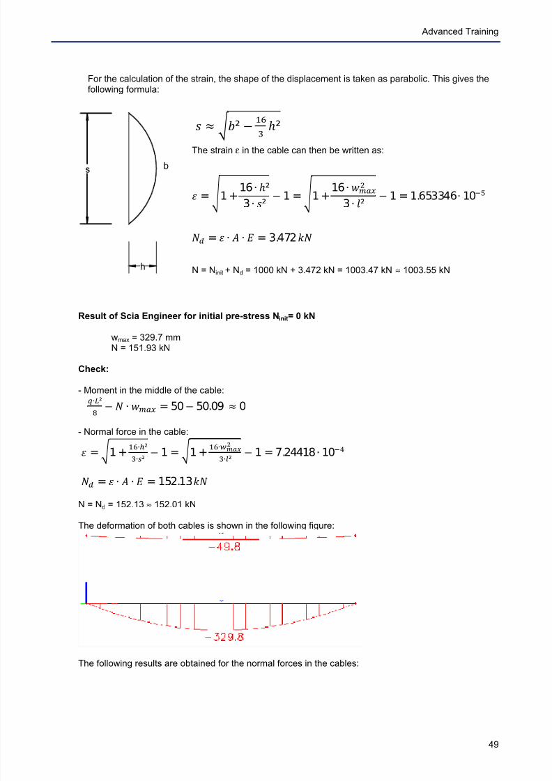
For the calculation of the strain, the shape of the displacement is taken as parabolic. This gives thefollowing formula:
s
h
b
I H J K²
OLMN O
²
The strain ε in the cable can then be written as:
P =Q 1 +16 + O²
3 + R² O 1 =S 1 +
16 + TUVWX3 + Y² O 1 = 1.653346 + 10Z[
\] = ^ + _ + ` = 3.472 bc
N = Ninit + Nd = 1000 kN + 3.472 kN = 1003.47 kN ≈ 1003.55 kN
Result of Scia Engineer for initial pre-stress Ninit= 0 kN
wmax = 329.7 mmN = 151.93 kN
Check:
- Moment in the middle of the cable:
d+e²
f O g + hijk = 50 O 50.09 H 0
- Normal force in the cable:
l =m 1 +no+p²q+r²
O 1 =s 1 +tu+vwxyz{+|² O 1 = 7.24418 + 10}~
• = ! + " + # = 152.13 %&
N = Nd = 152.13 ≈ 152.01 kN
The deformation of both cables is shown in the following figure:
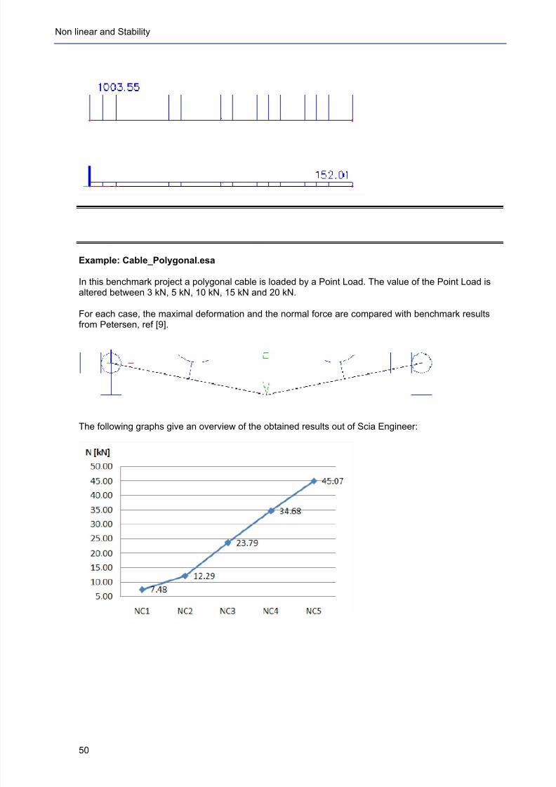
The following results are obtained for the normal forces in the cables:
7/18/2019 Nonlinear and Stability 2013
http://slidepdf.com/reader/full/nonlinear-and-stability-2013 54/106
Non linear and Stability
50
Example: Cable_Polygonal.esa
In this benchmark project a polygonal cable is loaded by a Point Load. The value of the Point Load isaltered between 3 kN, 5 kN, 10 kN, 15 kN and 20 kN.
For each case, the maximal deformation and the normal force are compared with benchmark resultsfrom Petersen, ref [9].
The following graphs give an overview of the obtained results out of Scia Engineer:
7/18/2019 Nonlinear and Stability 2013
http://slidepdf.com/reader/full/nonlinear-and-stability-2013 55/106
Advanced Training
51
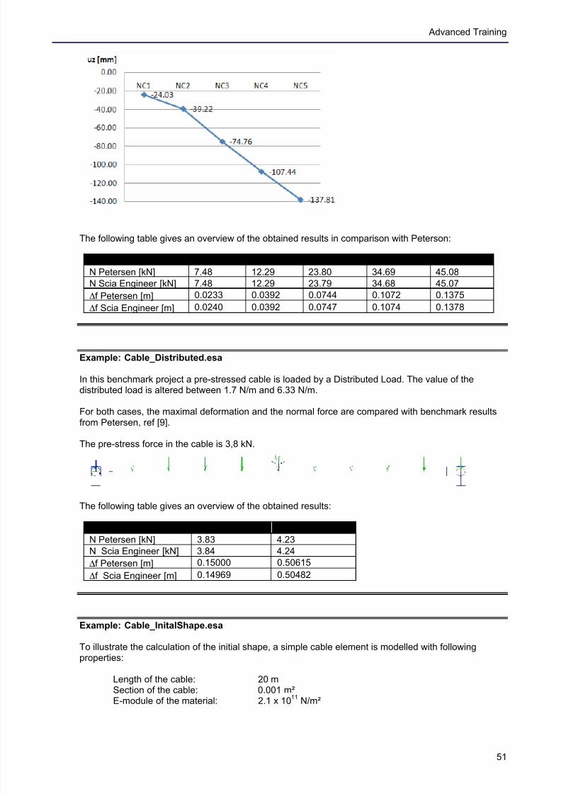
The following table gives an overview of the obtained results in comparison with Peterson:
F 3.0 kN 5.0 kN 10.0 kN 15.0 kN 20.0 kN
N Petersen [kN] 7.48 12.29 23.80 34.69 45.08
N Scia Engineer [kN] 7.48 12.29 23.79 34.68 45.07
∆f Petersen [m] 0.0233 0.0392 0.0744 0.1072 0.1375
∆f Scia Engineer [m] 0.0240 0.0392 0.0747 0.1074 0.1378
Example: Cable_Distributed.esa
In this benchmark project a pre-stressed cable is loaded by a Distributed Load. The value of thedistributed load is altered between 1.7 N/m and 6.33 N/m.
For both cases, the maximal deformation and the normal force are compared with benchmark resultsfrom Petersen, ref [9].
The pre-stress force in the cable is 3,8 kN.
The following table gives an overview of the obtained results:
q 1.7 N/m 6.33 N/m
N Petersen [kN] 3.83 4.23
N Scia Engineer [kN] 3.84 4.24
∆f Petersen [m] 0.15000 0.50615
∆f Scia Engineer [m] 0.14969 0.50482
Example: Cable_InitalShape.esa
To illustrate the calculation of the initial shape, a simple cable element is modelled with followingproperties:
Length of the cable: 20 mSection of the cable: 0.001 m²E-module of the material: 2.1 x 10¹¹ N/m²
7/18/2019 Nonlinear and Stability 2013
http://slidepdf.com/reader/full/nonlinear-and-stability-2013 56/106
Non linear and Stability
52
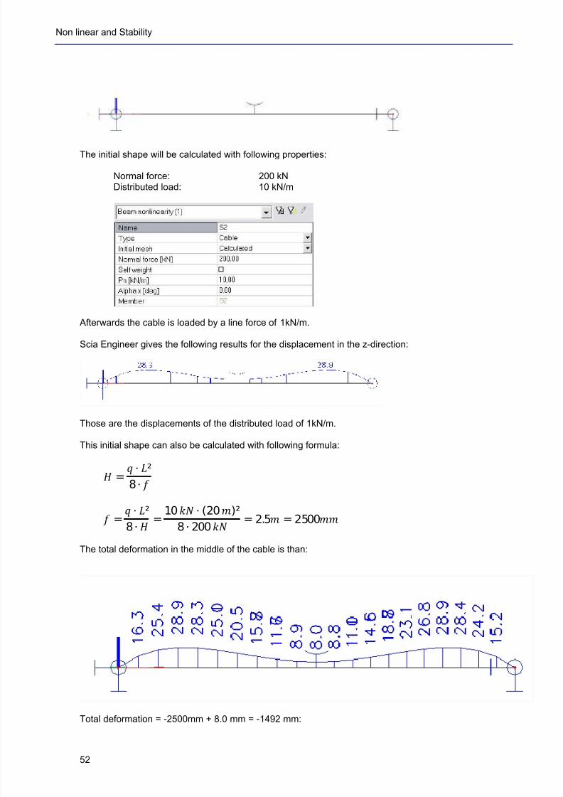
The initial shape will be calculated with following properties:
Normal force: 200 kNDistributed load: 10 kN/m
Afterwards the cable is loaded by a line force of 1kN/m.
Scia Engineer gives the following results for the displacement in the z-direction:
Those are the displacements of the distributed load of 1kN/m.
This initial shape can also be calculated with following formula:
' =( + )²
8 + *
+ =, + -²
8 + . =10 01 + (20 3)²
8 + 200 56 = 2.57 = 250089
The total deformation in the middle of the cable is than:
Total deformation = -2500mm + 8.0 mm = -1492 mm:
7/18/2019 Nonlinear and Stability 2013
http://slidepdf.com/reader/full/nonlinear-and-stability-2013 57/106
Advanced Training
53
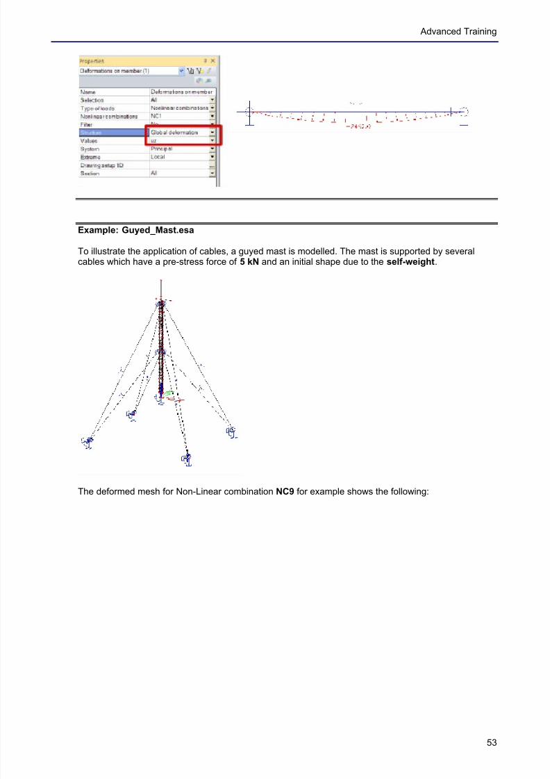
Example: Guyed_Mast.esa
To illustrate the application of cables, a guyed mast is modelled. The mast is supported by severalcables which have a pre-stress force of 5 kN and an initial shape due to the self-weight.
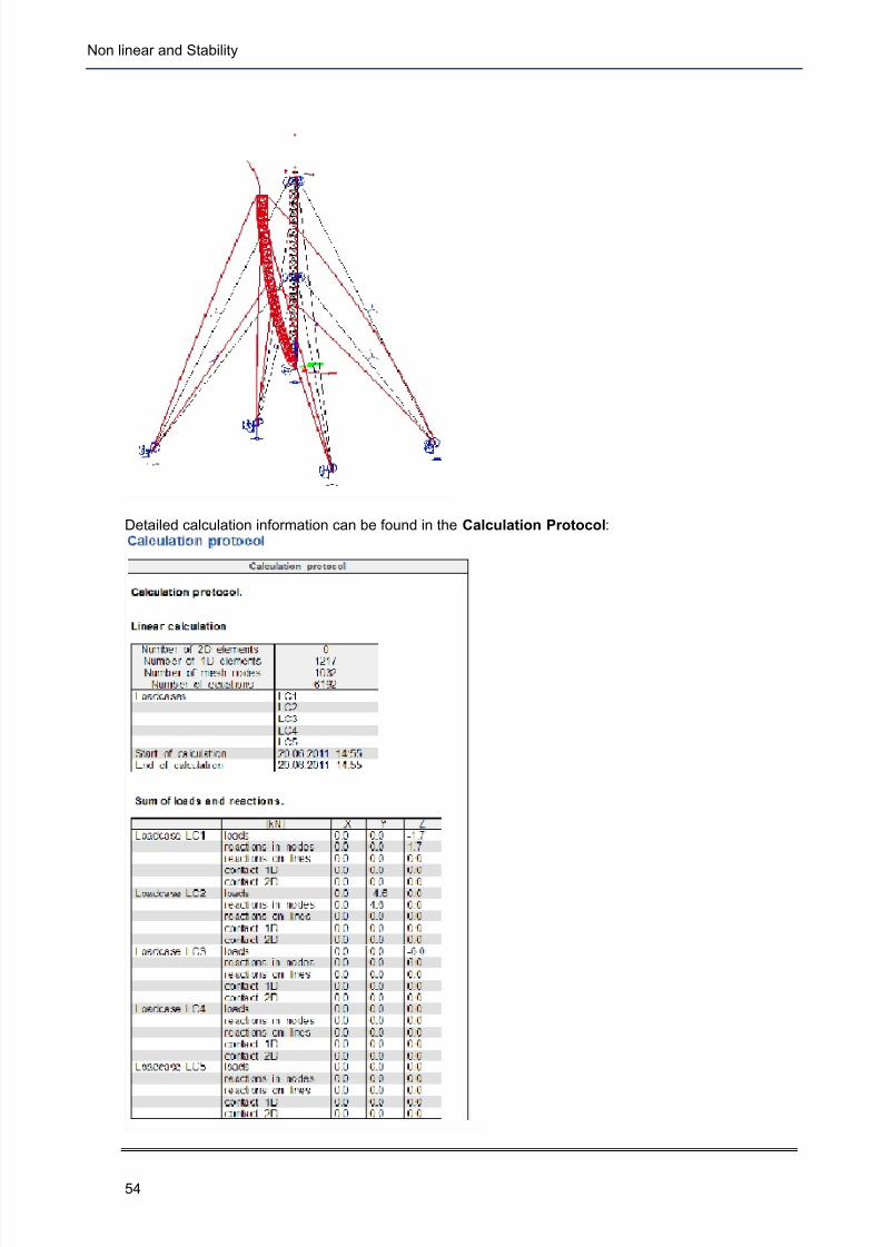
The deformed mesh for Non-Linear combination NC9 for example shows the following:
7/18/2019 Nonlinear and Stability 2013
http://slidepdf.com/reader/full/nonlinear-and-stability-2013 58/106
Non linear and Stability
54
Detailed calculation information can be found in the Calculation Protocol:
7/18/2019 Nonlinear and Stability 2013
http://slidepdf.com/reader/full/nonlinear-and-stability-2013 59/106
Advanced Training
55
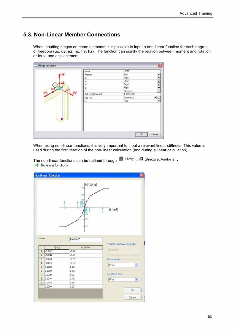
5.3. Non-Linear Member Connections
When inputting hinges on beam elements, it is possible to input a non-linear function for each degreeof freedom (ux, uy, uz, fix, fiy, fiz). The function can signify the relation between moment and rotationor force and displacement.
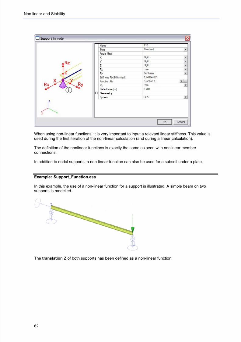
When using non-linear functions, it is very important to input a relevant linear stiffness. This value isused during the first iteration of the non-linear calculation (and during a linear calculation).
The non-linear functions can be defined through > >
7/18/2019 Nonlinear and Stability 2013
http://slidepdf.com/reader/full/nonlinear-and-stability-2013 60/106
Non linear and Stability
56
For member connections, the non-linear functions can be defined for translation or rotation. Whendefining a function, it is very important to check the signs of the function values. The definingmagnitudes for non-linear rotation functions are the internal forces, for non-linear translation functionsthe displacements.This implies that these functions are inputted in the first and third quadrant.
For the end of the function, it is possible to select one of three options:
- Free: When the maximal force is reached, it stays at that value and the deformation will riseuncontrolled.
- Fixed: When the maximal deformation is reached, it stays at that value and the force componentwill rise.
- Flexible: The relation between force component and deformation is linear.
Scia Engineer also allows creating a new function from the already defined functions to provide an
easy input of complex functions.
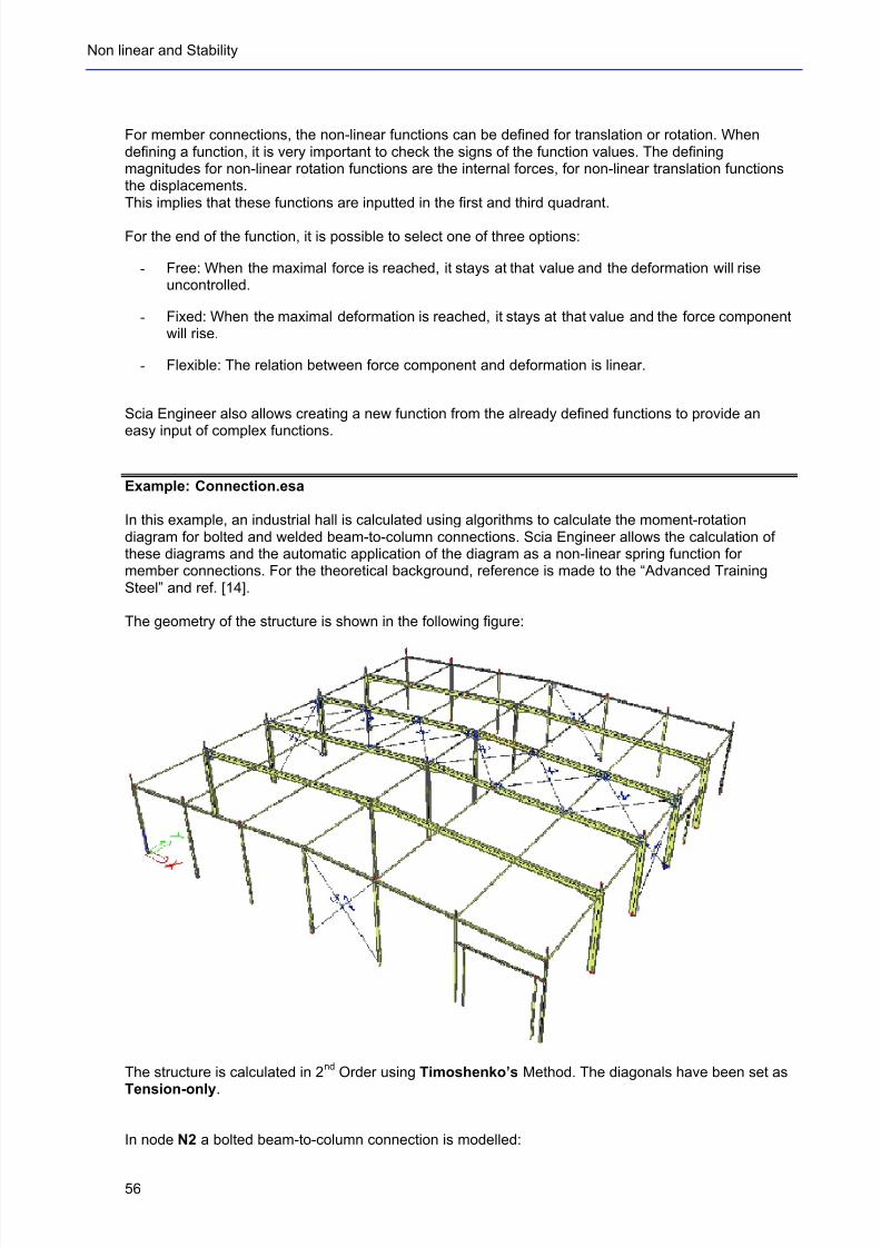
Example: Connection.esa
In this example, an industrial hall is calculated using algorithms to calculate the moment-rotationdiagram for bolted and welded beam-to-column connections. Scia Engineer allows the calculation ofthese diagrams and the automatic application of the diagram as a non-linear spring function formember connections. For the theoretical background, reference is made to the “Advanced TrainingSteel” and ref. [14].
The geometry of the structure is shown in the following figure:
The structure is calculated in 2nd
Order using Timoshenko’s Method. The diagonals have been set as
Tension-only.
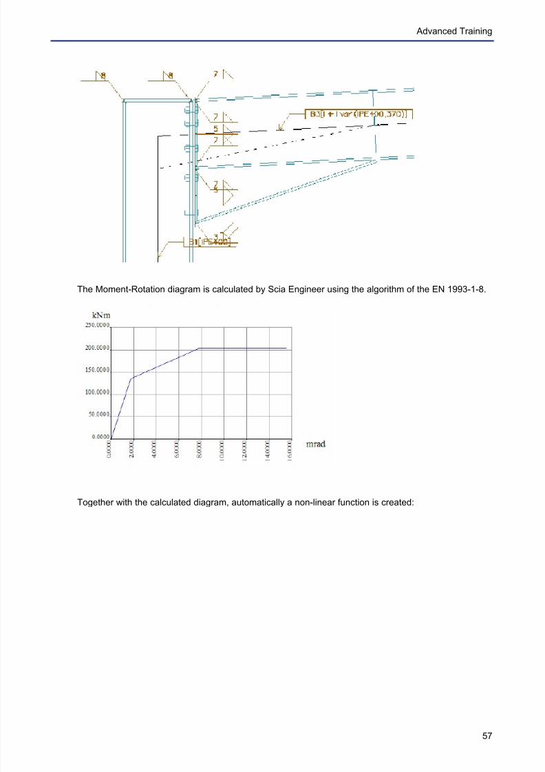
In node N2 a bolted beam-to-column connection is modelled:
7/18/2019 Nonlinear and Stability 2013
http://slidepdf.com/reader/full/nonlinear-and-stability-2013 61/106
Advanced Training
57
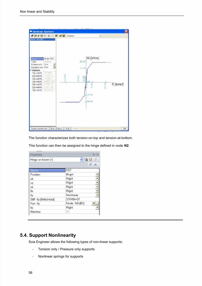
The Moment-Rotation diagram is calculated by Scia Engineer using the algorithm of the EN 1993-1-8.
Together with the calculated diagram, automatically a non-linear function is created:
7/18/2019 Nonlinear and Stability 2013
http://slidepdf.com/reader/full/nonlinear-and-stability-2013 62/106
Non linear and Stability
58
The function characterizes both tension-on-top and tension-at-bottom.
This function can then be assigned to the hinge defined in node N2:
5.4. Support Nonlinearity
Scia Engineer allows the following types of non-linear supports:
- Tension only / Pressure only supports
- Nonlinear springs for supports

7/18/2019 Nonlinear and Stability 2013
http://slidepdf.com/reader/full/nonlinear-and-stability-2013 63/106
Advanced Training
59
- Friction supports
5.4.1. Tension only / Pressure only Supports
To input nonlinearities for supports, the functionality Nonlinearity > Support nonlinearity must beactivated.
Supports with tension can be automatically eliminated. This is mostly used for slabs on subsoil, columnbases of for example scaffoldings, struts, …
The following types of supports can be eliminated if tension occurs:
- Nodal Support
- Line Support
- Subsoil
For Nodal Supports or Line Supports it is possible to specify a translation degree of freedom as ‘Rigidpressure only’ or ‘Flexible Pressure only’.
To eliminate supports in pressure (and obtain a Tension-only support), the nodal support can be
rotated 180°.
Subsoils are always regarded as Pressure-only for a non-linear calculation. No specific input has to
be made.
7/18/2019 Nonlinear and Stability 2013
http://slidepdf.com/reader/full/nonlinear-and-stability-2013 64/106
Non linear and Stability
60
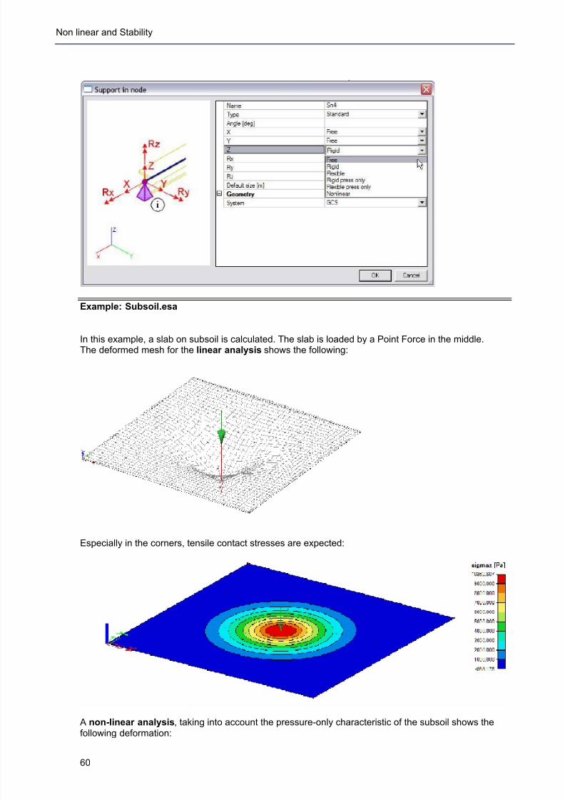
Example: Subsoil.esa
In this example, a slab on subsoil is calculated. The slab is loaded by a Point Force in the middle.The deformed mesh for the linear analysis shows the following:
Especially in the corners, tensile contact stresses are expected:
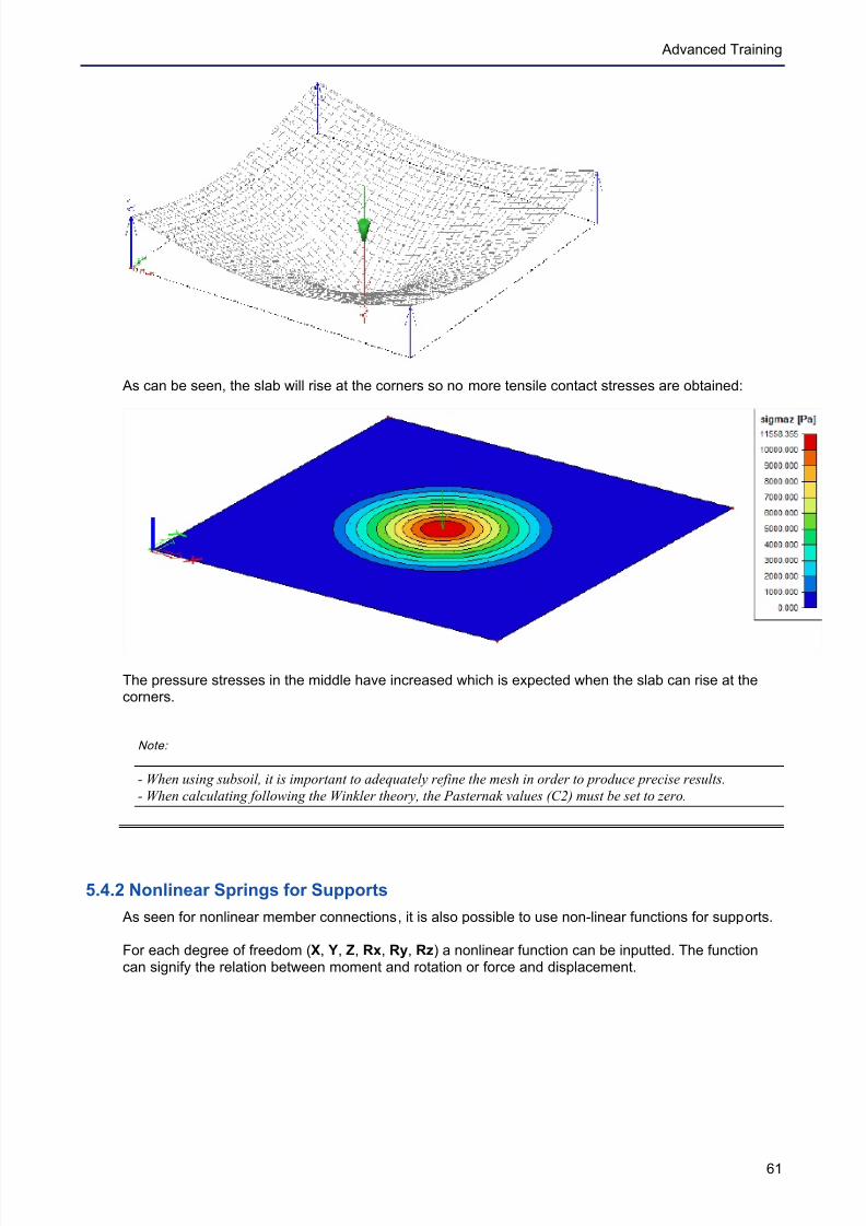
A non-linear analysis, taking into account the pressure-only characteristic of the subsoil shows thefollowing deformation:
7/18/2019 Nonlinear and Stability 2013
http://slidepdf.com/reader/full/nonlinear-and-stability-2013 65/106
Advanced Training
61
As can be seen, the slab will rise at the corners so no more tensile contact stresses are obtained:
The pressure stresses in the middle have increased which is expected when the slab can rise at thecorners.
Note:
- When using subsoil, it is important to adequately refine the mesh in order to produce precise results.
- When calculating following the Winkler theory, the Pasternak values (C2) must be set to zero.
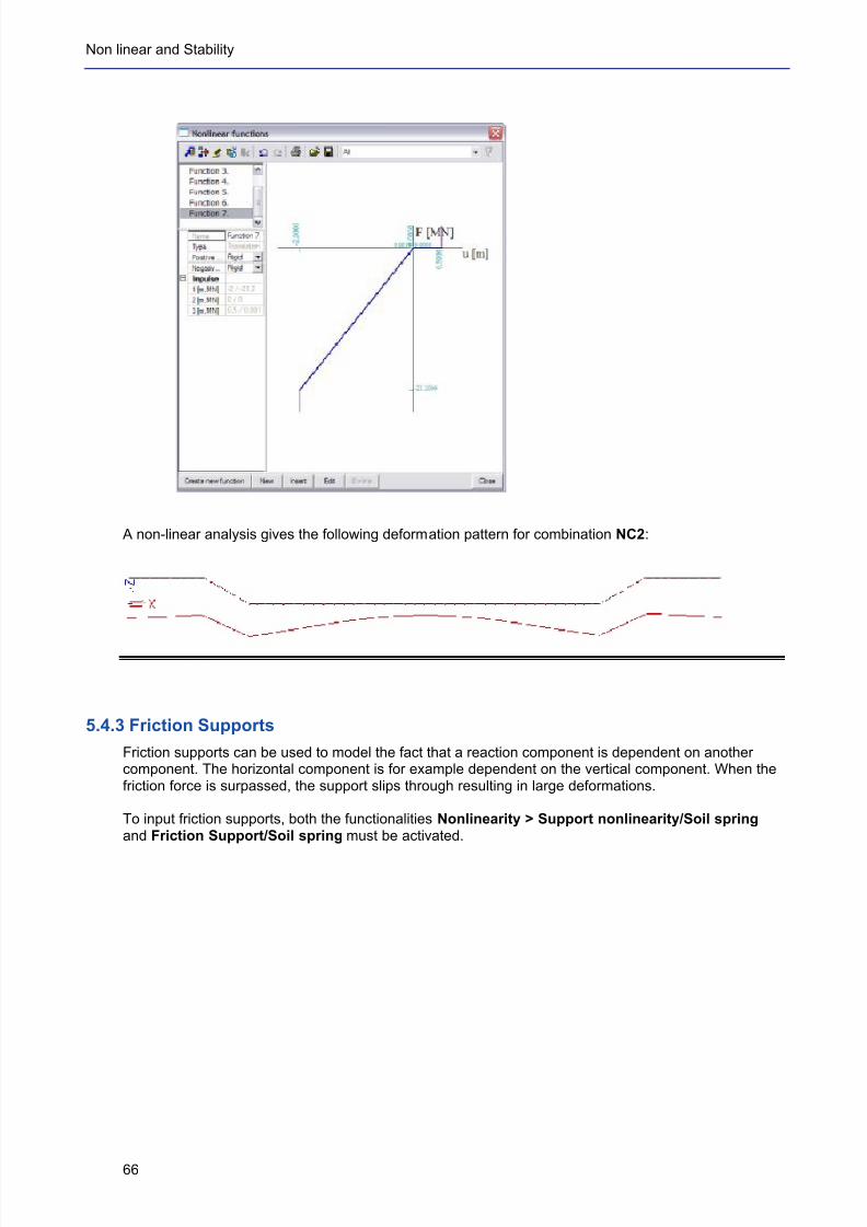
5.4.2 Nonlinear Springs for Supports
As seen for nonlinear member connections, it is also possible to use non-linear functions for supports.
For each degree of freedom (X, Y, Z, Rx, Ry, Rz) a nonlinear function can be inputted. The functioncan signify the relation between moment and rotation or force and displacement.
7/18/2019 Nonlinear and Stability 2013
http://slidepdf.com/reader/full/nonlinear-and-stability-2013 66/106
7/18/2019 Nonlinear and Stability 2013
http://slidepdf.com/reader/full/nonlinear-and-stability-2013 67/106
Advanced Training
63
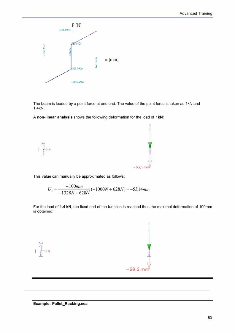
The beam is loaded by a point force at one end. The value of the point force is taken as 1kN and1.4kN.
A non-linear analysis shows the following deformation for the load of 1kN:
This value can manually be approximated as follows:
mm N N N
mmU z 14,53)6281000(
6281328
100−=+−
+−
−=
For the load of 1.4 kN, the fixed end of the function is reached thus the maximal deformation of 100mmis obtained:
Example: Pallet_Racking.esa
7/18/2019 Nonlinear and Stability 2013
http://slidepdf.com/reader/full/nonlinear-and-stability-2013 68/106
Non linear and Stability
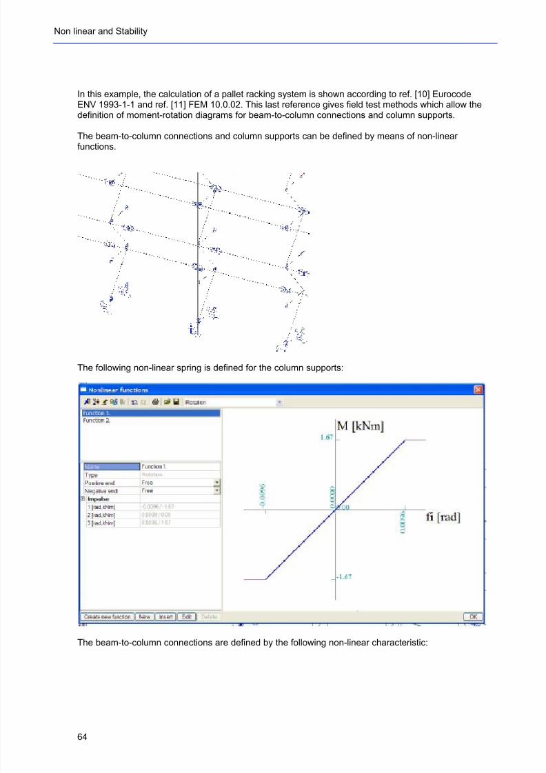
64
In this example, the calculation of a pallet racking system is shown according to ref. [10] EurocodeENV 1993-1-1 and ref. [11] FEM 10.0.02. This last reference gives field test methods which allow thedefinition of moment-rotation diagrams for beam-to-column connections and column supports.
The beam-to-column connections and column supports can be defined by means of non-linearfunctions.
The following non-linear spring is defined for the column supports:
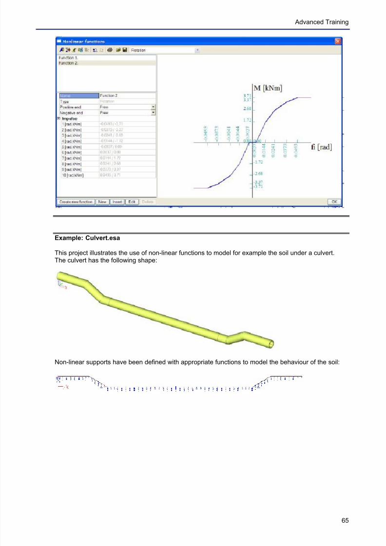
The beam-to-column connections are defined by the following non-linear characteristic:
7/18/2019 Nonlinear and Stability 2013
http://slidepdf.com/reader/full/nonlinear-and-stability-2013 69/106
Advanced Training
65
Example: Culvert.esa
This project illustrates the use of non-linear functions to model for example the soil under a culvert.The culvert has the following shape:
Non-linear supports have been defined with appropriate functions to model the behaviour of the soil:
7/18/2019 Nonlinear and Stability 2013
http://slidepdf.com/reader/full/nonlinear-and-stability-2013 70/106
Non linear and Stability
66
A non-linear analysis gives the following deformation pattern for combination NC2:
5.4.3 Friction Supports
Friction supports can be used to model the fact that a reaction component is dependent on anothercomponent. The horizontal component is for example dependent on the vertical component. When thefriction force is surpassed, the support slips through resulting in large deformations.
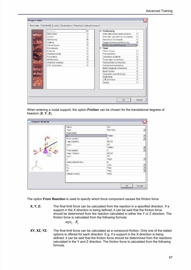
To input friction supports, both the functionalities Nonlinearity > Support nonlinearity/Soil springand Friction Support/Soil spring must be activated.
7/18/2019 Nonlinear and Stability 2013
http://slidepdf.com/reader/full/nonlinear-and-stability-2013 71/106
Advanced Training
67
When entering a nodal support, the option Friction can be chosen for the translational degrees offreedom (X, Y, Z).
The option From Reaction is used to specify which force component causes the friction force.
X, Y, Z: The final limit force can be calculated from the reaction in a specified direction. If asupport in the X-direction is being defined, it can be said that the friction forceshould be determined from the reaction calculated in either the Y or Z direction. Thefriction force is calculated from the following formula:
z x Rmju ⋅
XY, XZ, YZ: The final limit force can be calculated as a compound friction. Only one of the statedoptions is offered for each direction. E.g. if a support in the X-direction is beingdefined, it can be said that the friction force should be determined from the reactionscalculated in the Y and Z direction. The friction force is calculated from the followingformula:
7/18/2019 Nonlinear and Stability 2013
http://slidepdf.com/reader/full/nonlinear-and-stability-2013 72/106
Non linear and Stability
68
22
z y x R Rmju +⋅
X+Y, X+Z, Y+Z: The same as above applies here. A different procedure is however used tocalculate the limit force. E.g. for a friction support in the X-direction the following
formula is employed:
z x y x Rmju Rmju ⋅+⋅
In these formulas, mju specifies the coefficient of friction.
In the field C flex, the stiffness of the support can be inputted.
Note:
- Friction can be inputted in one or two directions. It is not possible to define friction in all three directions since otherwise the "thrust" cannot be determined.
- When simple friction (X, Y, Z) is defined in two directions, the option Independent is available. This specifiesthat the friction in one direction is independent on the friction in the other direction.
- Composed friction (e.g. YZ or Y+Z) can be specified only in one direction.
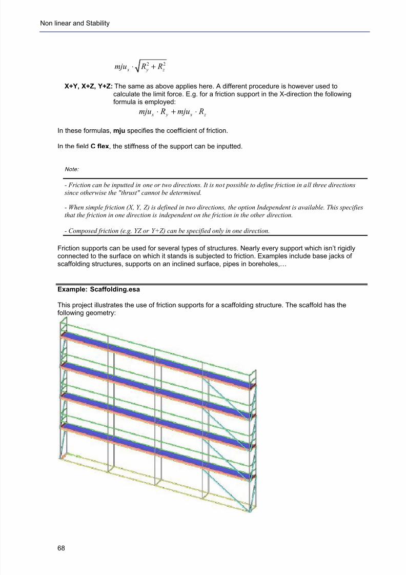
Friction supports can be used for several types of structures. Nearly every support which isn’t rigidlyconnected to the surface on which it stands is subjected to friction. Examples include base jacks ofscaffolding structures, supports on an inclined surface, pipes in boreholes,…
Example: Scaffolding.esa
This project illustrates the use of friction supports for a scaffolding structure. The scaffold has thefollowing geometry:
7/18/2019 Nonlinear and Stability 2013
http://slidepdf.com/reader/full/nonlinear-and-stability-2013 73/106
Advanced Training
69
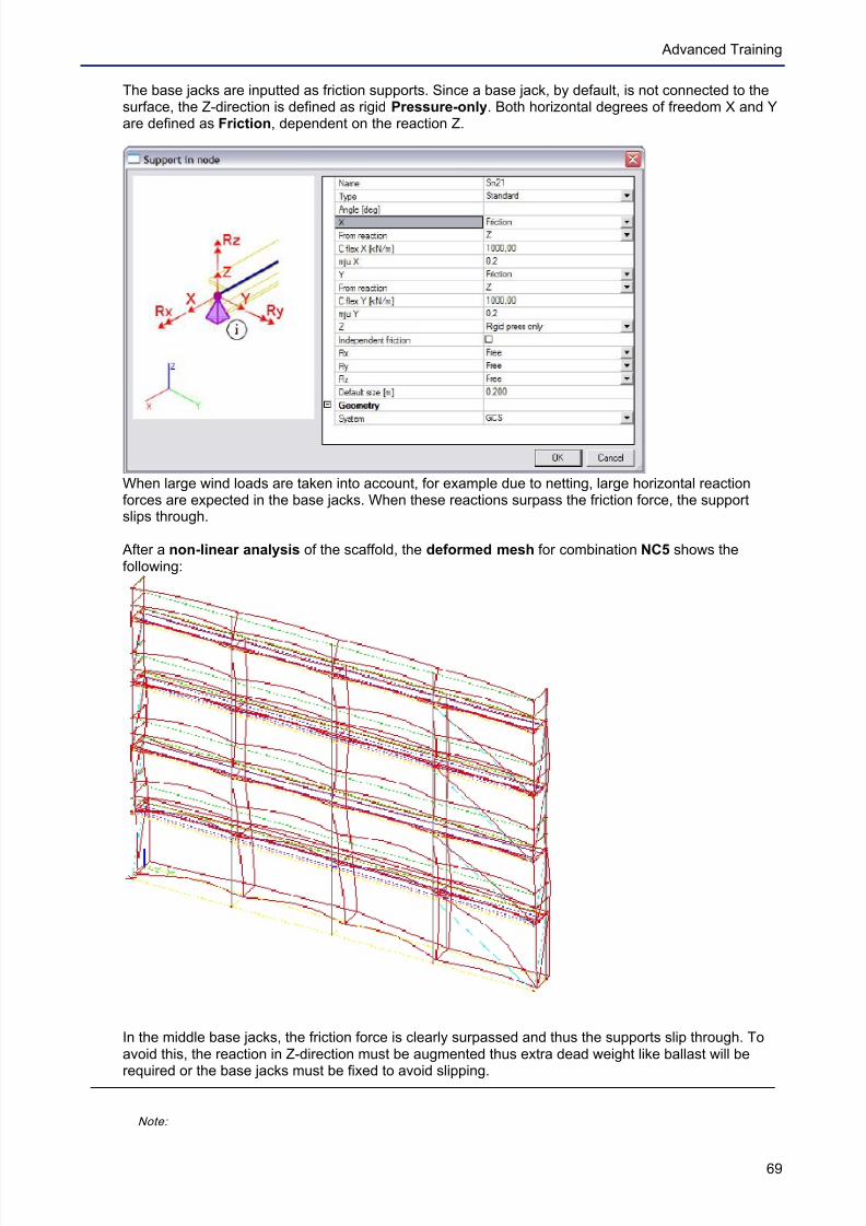
The base jacks are inputted as friction supports. Since a base jack, by default, is not connected to thesurface, the Z-direction is defined as rigid Pressure-only. Both horizontal degrees of freedom X and Yare defined as Friction, dependent on the reaction Z.
When large wind loads are taken into account, for example due to netting, large horizontal reactionforces are expected in the base jacks. When these reactions surpass the friction force, the supportslips through.
After a non-linear analysis of the scaffold, the deformed mesh for combination NC5 shows thefollowing:
In the middle base jacks, the friction force is clearly surpassed and thus the supports slip through. Toavoid this, the reaction in Z-direction must be augmented thus extra dead weight like ballast will be
required or the base jacks must be fixed to avoid slipping.
Note:
7/18/2019 Nonlinear and Stability 2013
http://slidepdf.com/reader/full/nonlinear-and-stability-2013 74/106
Non linear and Stability
70
The functionality ‘Nonlinear Line Support’ defines a specific type of soil spring developed for the Pipfas
project (Buried Pipe Design).
5.5 2D Elements
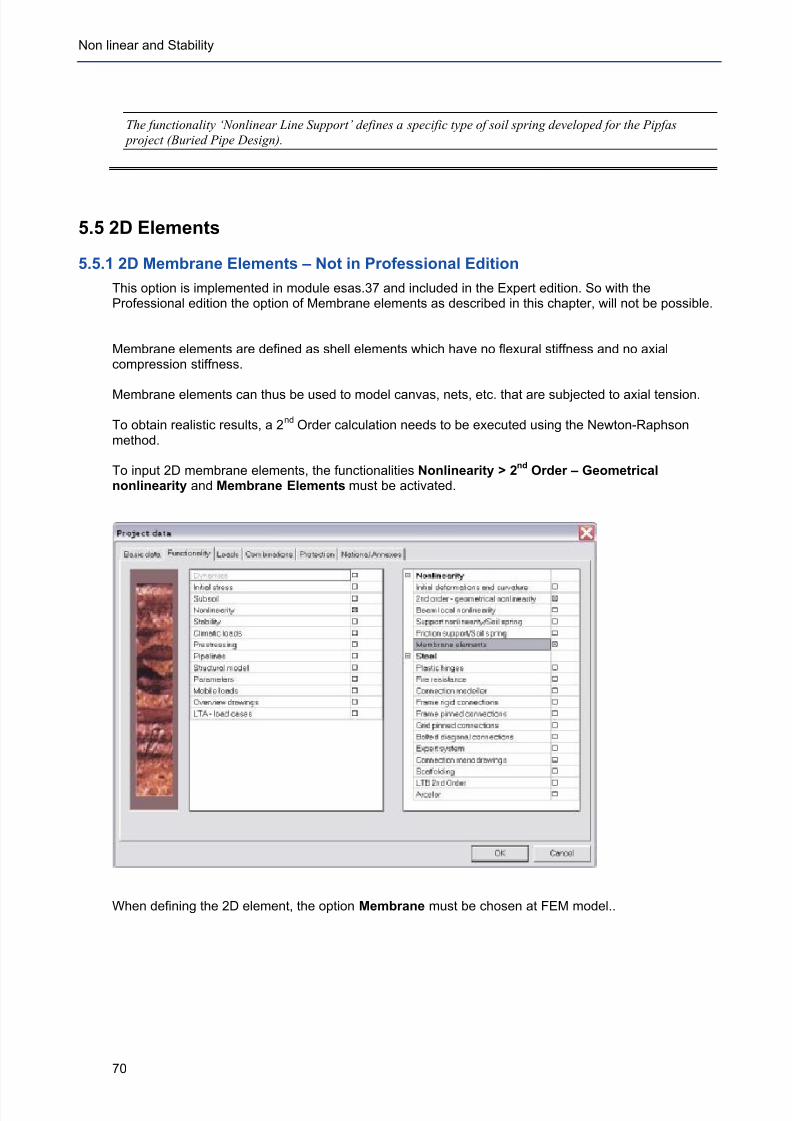
5.5.1 2D Membrane Elements – Not in Professional Edition
This option is implemented in module esas.37 and included in the Expert edition. So with theProfessional edition the option of Membrane elements as described in this chapter, will not be possible.
Membrane elements are defined as shell elements which have no flexural stiffness and no axialcompression stiffness.
Membrane elements can thus be used to model canvas, nets, etc. that are subjected to axial tension.
To obtain realistic results, a 2nd
Order calculation needs to be executed using the Newton-Raphsonmethod.
To input 2D membrane elements, the functionalities Nonlinearity > 2nd
Order – Geometricalnonlinearity and Membrane Elements must be activated.
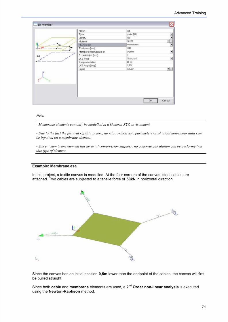
When defining the 2D element, the option Membrane must be chosen at FEM model..
7/18/2019 Nonlinear and Stability 2013
http://slidepdf.com/reader/full/nonlinear-and-stability-2013 75/106
Advanced Training
71
Note:
- Membrane elements can only be modelled in a General XYZ environment.
- Due to the fact the flexural rigidity is zero, no ribs, orthotropic parameters or physical non-linear data can
be inputted on a membrane element.
- Since a membrane element has no axial compression stiffness, no concrete calculation can be performed on
this type of element.
Example: Membrane.esa
In this project, a textile canvas is modelled. At the four corners of the canvas, steel cables areattached. Two cables are subjected to a tensile force of 50kN in horizontal direction.
Since the canvas has an initial position 0,5m lower than the endpoint of the cables, the canvas will first
be pulled straight.
Since both cable and membrane elements are used, a 2nd
Order non-linear analysis is executedusing the Newton-Raphson method.
7/18/2019 Nonlinear and Stability 2013
http://slidepdf.com/reader/full/nonlinear-and-stability-2013 76/106
Non linear and Stability
72
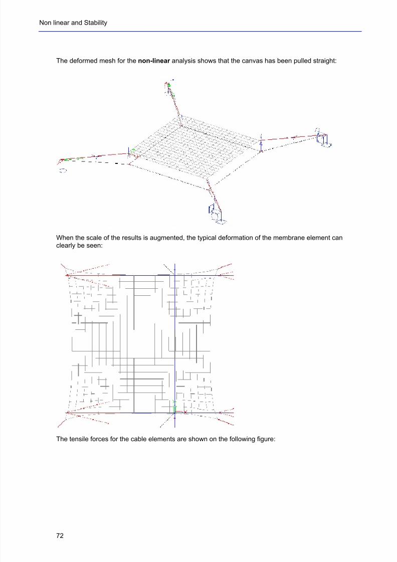
The deformed mesh for the non-linear analysis shows that the canvas has been pulled straight:
When the scale of the results is augmented, the typical deformation of the membrane element canclearly be seen:
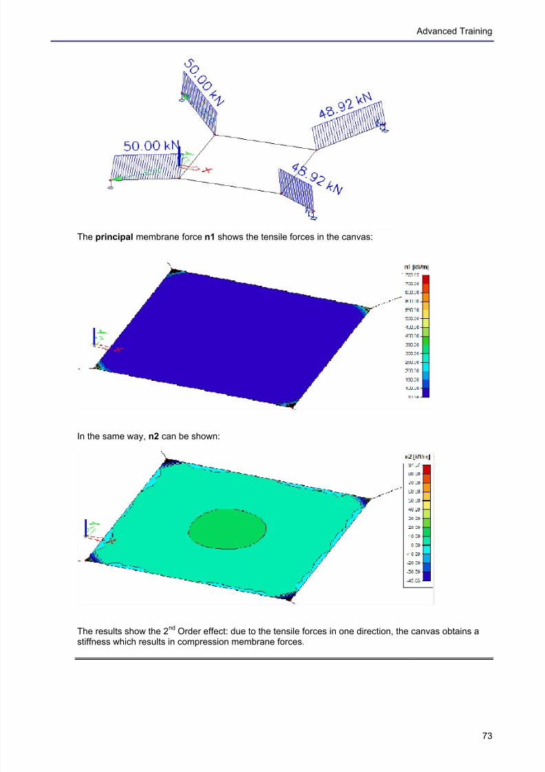
The tensile forces for the cable elements are shown on the following figure:
7/18/2019 Nonlinear and Stability 2013
http://slidepdf.com/reader/full/nonlinear-and-stability-2013 77/106
Advanced Training
73
The principal membrane force n1 shows the tensile forces in the canvas:
In the same way, n2 can be shown:
The results show the 2nd
Order effect: due to the tensile forces in one direction, the canvas obtains astiffness which results in compression membrane forces.
7/18/2019 Nonlinear and Stability 2013
http://slidepdf.com/reader/full/nonlinear-and-stability-2013 78/106
Non linear and Stability
74
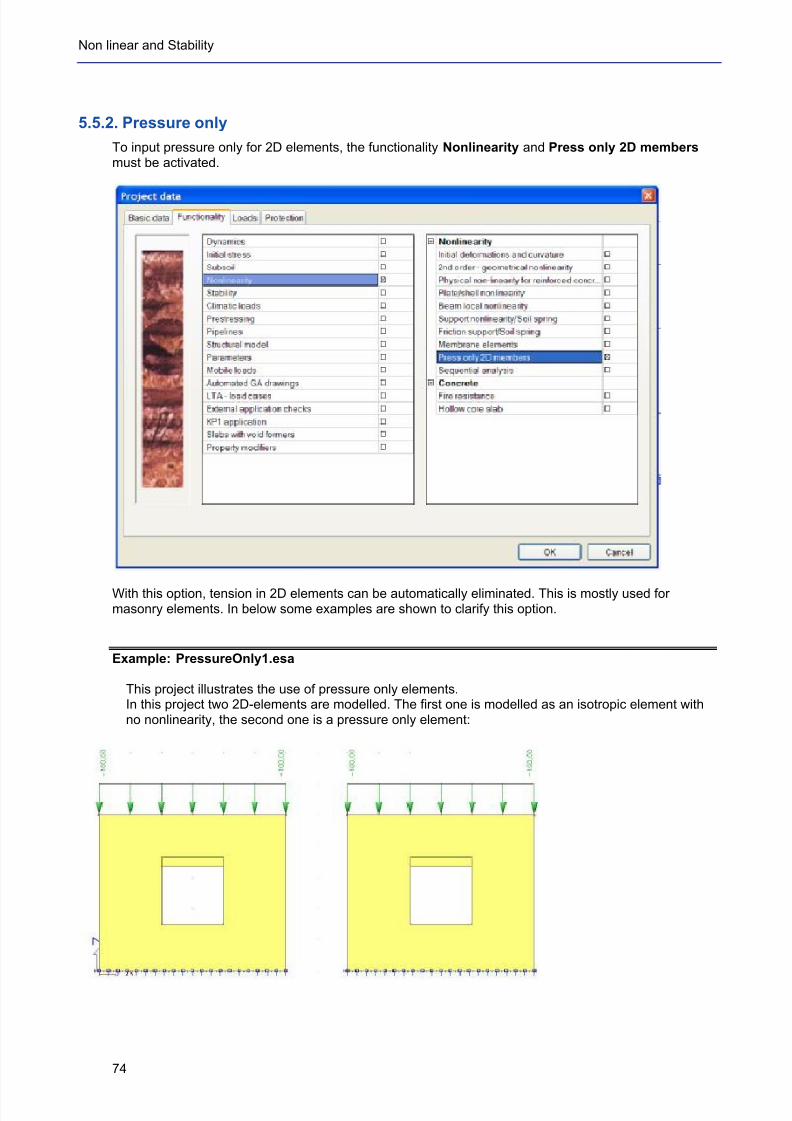
5.5.2. Pressure only
To input pressure only for 2D elements, the functionality Nonlinearity and Press only 2D membersmust be activated.
With this option, tension in 2D elements can be automatically eliminated. This is mostly used formasonry elements. In below some examples are shown to clarify this option.
Example: PressureOnly1.esa
This project illustrates the use of pressure only elements.In this project two 2D-elements are modelled. The first one is modelled as an isotropic element withno nonlinearity, the second one is a pressure only element:
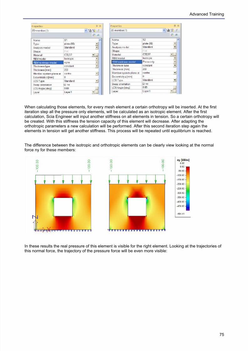
7/18/2019 Nonlinear and Stability 2013
http://slidepdf.com/reader/full/nonlinear-and-stability-2013 79/106
Advanced Training
75
When calculating those elements, for every mesh element a certain orthotropy will be inserted. At the firstiteration step all the pressure only elements, will be calculated as an isotropic element. After the firstcalculation, Scia Engineer will input another stiffness on all elements in tension. So a certain orthotropy will
be created. With this stiffness the tension capacity of this element will decrease. After adapting theorthotropic parameters a new calculation will be performed. After this second iteration step again theelements in tension will get another stiffness. This process will be repeated until equilibrium is reached.
The difference between the isotropic and orthotropic elements can be clearly view looking at the normalforce ny for these members:
In these results the real pressure of this element is visible for the right element. Looking at the trajectories ofthis normal force, the trajectory of the pressure force will be even more visible:
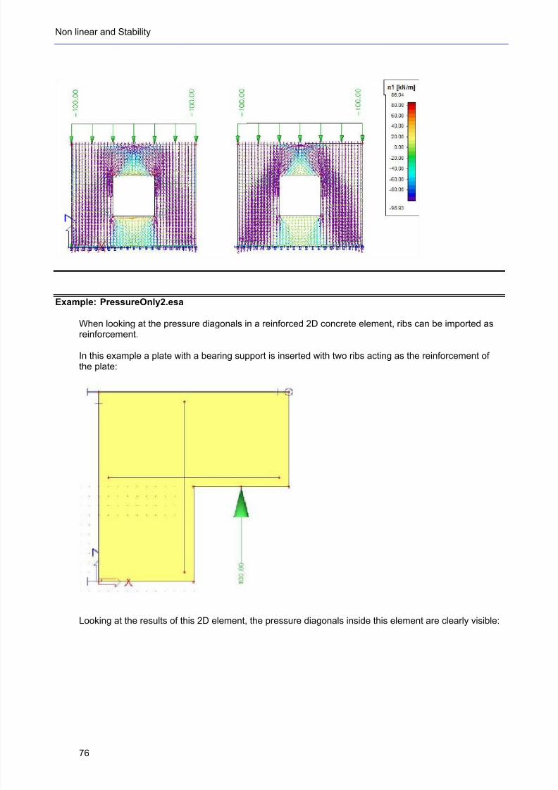
7/18/2019 Nonlinear and Stability 2013
http://slidepdf.com/reader/full/nonlinear-and-stability-2013 80/106
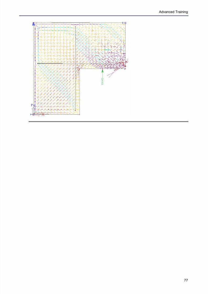
7/18/2019 Nonlinear and Stability 2013
http://slidepdf.com/reader/full/nonlinear-and-stability-2013 81/106
Advanced Training
77
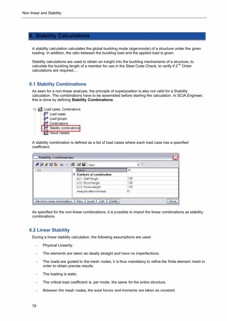
7/18/2019 Nonlinear and Stability 2013
http://slidepdf.com/reader/full/nonlinear-and-stability-2013 82/106
Non linear and Stability
78
6. Stability Calculations
A stability calculation calculates the global buckling mode (eigenmode) of a structure under the givenloading. In addition, the ratio between the buckling load and the applied load is given.
Stability calculations are used to obtain an insight into the buckling mechanisms of a structure, tocalculate the buckling length of a member for use in the Steel Code Check, to verify if 2
nd Order
calculations are required,…
6.1 Stability Combinations
As seen for a non-linear analysis, the principle of superposition is also not valid for a Stabilitycalculation. The combinations have to be assembled before starting the calculation. In SCIA.Engineer,this is done by defining Stability Combinations.
A stability combination is defined as a list of load cases where each load case has a specifiedcoefficient.
As specified for the non-linear combinations, it is possible to import the linear combinations as stabilitycombinations.
6.2 Linear Stability
During a linear stability calculation, the following assumptions are used:
- Physical Linearity.
- The elements are taken as ideally straight and have no imperfections.
- The loads are guided to the mesh nodes, it is thus mandatory to refine the finite element mesh inorder to obtain precise results.
- The loading is static.
- The critical load coefficient is, per mode, the same for the entire structure.
- Between the mesh nodes, the axial forces and moments are taken as constant.
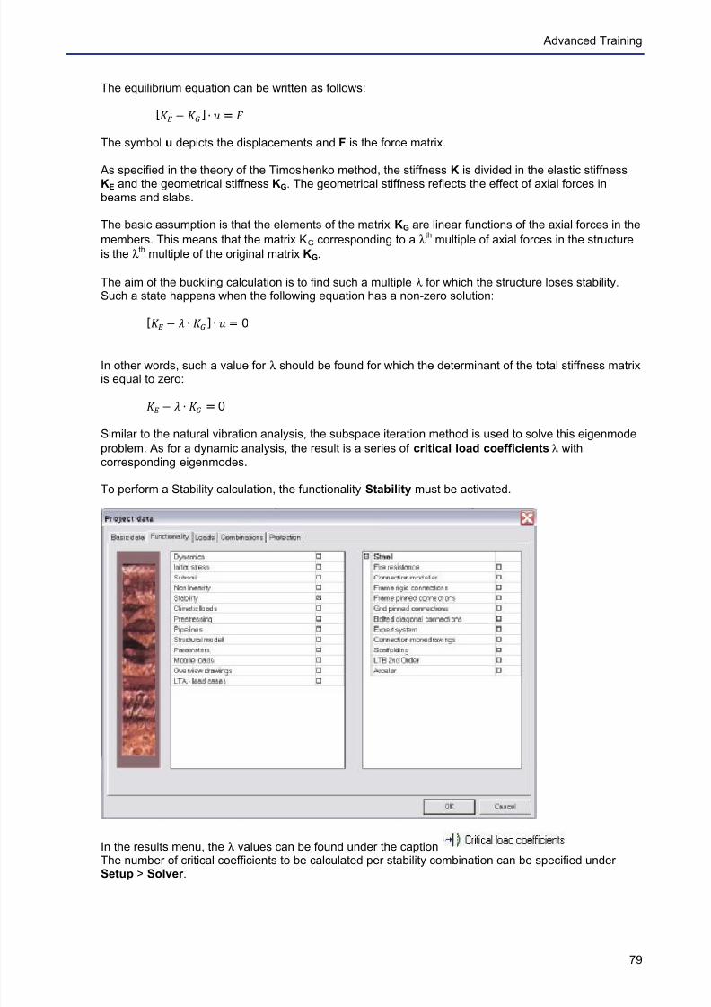
7/18/2019 Nonlinear and Stability 2013
http://slidepdf.com/reader/full/nonlinear-and-stability-2013 83/106
Advanced Training
79
The equilibrium equation can be written as follows:
[:; O <=] + > = ?
The symbol u depicts the displacements and F is the force matrix.
As specified in the theory of the Timoshenko method, the stiffness K is divided in the elastic stiffnessKE and the geometrical stiffness KG. The geometrical stiffness reflects the effect of axial forces inbeams and slabs.
The basic assumption is that the elements of the matrix KG are linear functions of the axial forces in the
members. This means that the matrix KG corresponding to a λth multiple of axial forces in the structure
is the λth multiple of the original matrix KG.
The aim of the buckling calculation is to find such a multiple λ for which the structure loses stability.Such a state happens when the following equation has a non-zero solution:
[@A O B + CD] + E = 0
In other words, such a value for λ should be found for which the determinant of the total stiffness matrixis equal to zero:
FG O H + IJ = 0
Similar to the natural vibration analysis, the subspace iteration method is used to solve this eigenmode
problem. As for a dynamic analysis, the result is a series of critical load coefficients λ withcorresponding eigenmodes.
To perform a Stability calculation, the functionality Stability must be activated.
In the results menu, the λ values can be found under the captionThe number of critical coefficients to be calculated per stability combination can be specified underSetup > Solver .
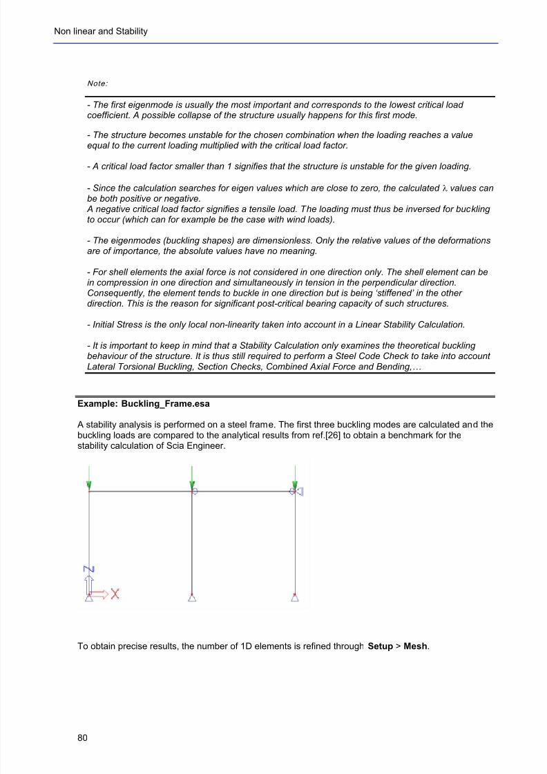
7/18/2019 Nonlinear and Stability 2013
http://slidepdf.com/reader/full/nonlinear-and-stability-2013 84/106
Non linear and Stability
80
Note:
- The first eigenmode is usually the most important and corresponds to the lowest critical loadcoefficient. A possible collapse of the structure usually happens for this first mode.
- The structure becomes unstable for the chosen combination when the loading reaches a valueequal to the current loading multiplied with the critical load factor.
- A critical load factor smaller than 1 signifies that the structure is unstable for the given loading.
- Since the calculation searches for eigen values which are close to zero, the calculated λ values canbe both positive or negative. A negative critical load factor signifies a tensile load. The loading must thus be inversed for bucklingto occur (which can for example be the case with wind loads).
- The eigenmodes (buckling shapes) are dimensionless. Only the relative values of the deformationsare of importance, the absolute values have no meaning.
- For shell elements the axial force is not considered in one direction only. The shell element can bein compression in one direction and simultaneously in tension in the perpendicular direction.Consequently, the element tends to buckle in one direction but is being ‘stiffened’ in the otherdirection. This is the reason for significant post-critical bearing capacity of such structures.
- Initial Stress is the only local non-linearity taken into account in a Linear Stability Calculation.
- It is important to keep in mind that a Stability Calculation only examines the theoretical bucklingbehaviour of the structure. It is thus still required to perform a Steel Code Check to take into accountLateral Torsional Buckling, Section Checks, Combined Axial Force and Bending,…
Example: Buckling_Frame.esa
A stability analysis is performed on a steel frame. The first three buckling modes are calculated and thebuckling loads are compared to the analytical results from ref.[26] to obtain a benchmark for thestability calculation of Scia Engineer.
To obtain precise results, the number of 1D elements is refined through Setup > Mesh.
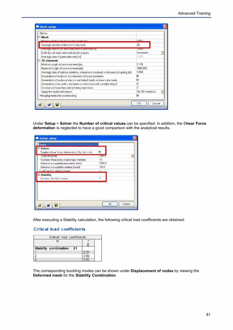
7/18/2019 Nonlinear and Stability 2013
http://slidepdf.com/reader/full/nonlinear-and-stability-2013 85/106
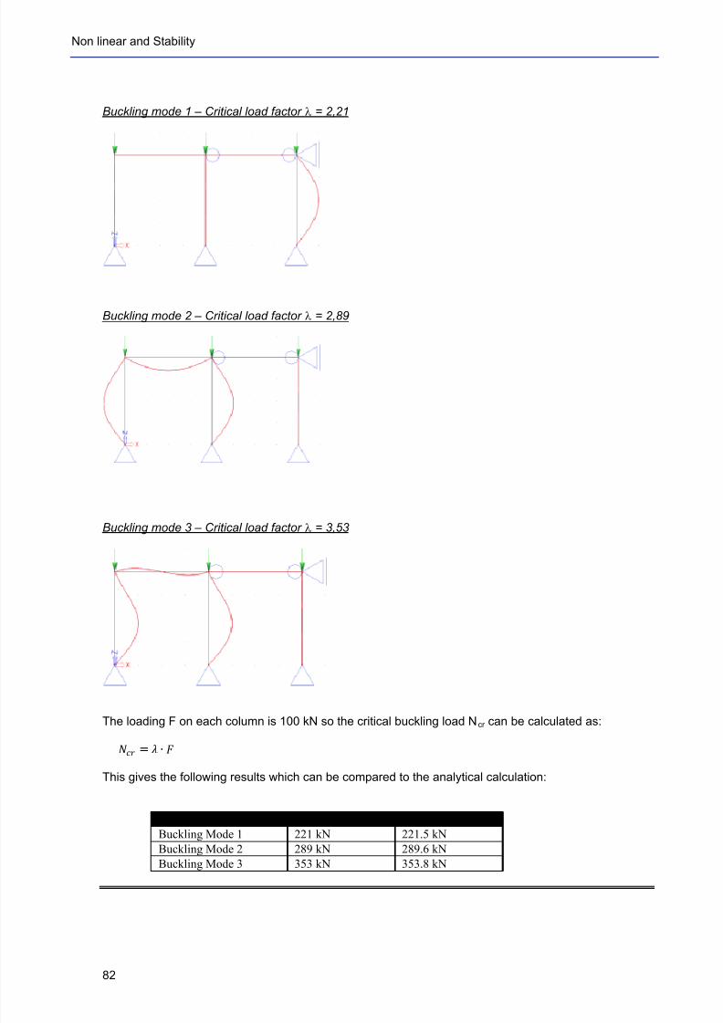
7/18/2019 Nonlinear and Stability 2013
http://slidepdf.com/reader/full/nonlinear-and-stability-2013 86/106
Non linear and Stability
82
Buckling mode 1 – Critical load factor λ = 2,21
Buckling mode 2 – Critical load factor λ = 2,89
Buckling mode 3 – Critical load factor λ = 3,53
The loading F on each column is 100 kN so the critical buckling load Ncr can be calculated as:
KLM = N + O
This gives the following results which can be compared to the analytical calculation:
Ncr for Scia Engineer Ref.[26]
Buckling Mode 1 221 kN 221.5 kN
Buckling Mode 2 289 kN 289.6 kN
Buckling Mode 3 353 kN 353.8 kN
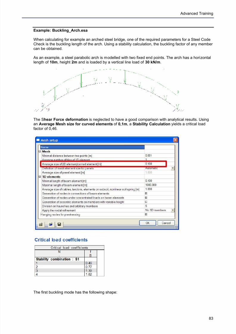
7/18/2019 Nonlinear and Stability 2013
http://slidepdf.com/reader/full/nonlinear-and-stability-2013 87/106
Advanced Training
83
Example: Buckling_Arch.esa
When calculating for example an arched steel bridge, one of the required parameters for a Steel CodeCheck is the buckling length of the arch. Using a stability calculation, the buckling factor of any membercan be obtained.
As an example, a steel parabolic arch is modelled with two fixed end points. The arch has a horizontallength of 10m, height 2m and is loaded by a vertical line load of 30 kN/m.
The Shear Force deformation is neglected to have a good comparison with analytical results. Usingan Average Mesh size for curved elements of 0,1m, a Stability Calculation yields a critical load
factor of 0,46.
The first buckling mode has the following shape:
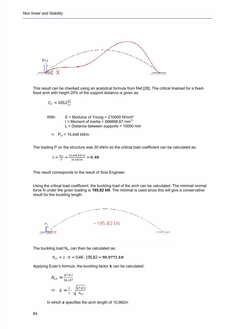
7/18/2019 Nonlinear and Stability 2013
http://slidepdf.com/reader/full/nonlinear-and-stability-2013 88/106
Non linear and Stability
84
This result can be checked using an analytical formula from Ref.[28]. The critical lineload for a fixed-fixed arch with height 20% of the support distance is given as:
PQR = 103,2ST
U³
With: E = Modulus of Young = 210000 N/mm²I = Moment of inertia = 666666,67 mm
4
L = Distance between supports = 10000 mm
ð Pcr = 14,448 kN/m
The loading P on the structure was 30 kN/m so the critical load coefficient can be calculated as:
V =WXY
Z=
[\,]^_ ab/c
de gh/i=j,kl
This result corresponds to the result of Scia Engineer.
Using the critical load coefficient, the buckling load of the arch can be calculated. The minimal normalforce N under the given loading is 195,82 kN. The minimal is used since this will give a conservativeresult for the buckling length.
The buckling load Ncr can then be calculated as:
mno = p + q = 0,46 + 195,82 = rs,tuvw yz
Applying Euler’s formula, the buckling factor k can be calculated:
{|} =~²+•+(!+")#
ð $ = %& + ' (²+)+*+,-
In which s specifies the arch length of 10,982m
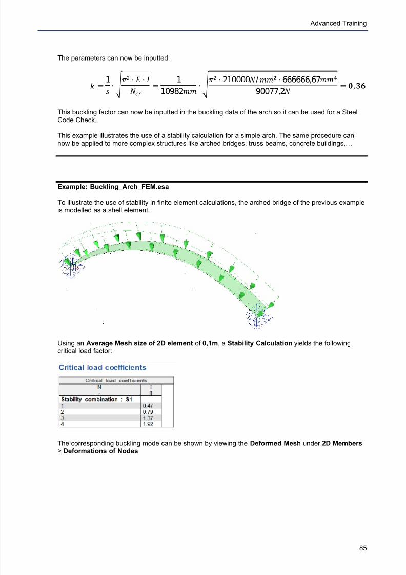
7/18/2019 Nonlinear and Stability 2013
http://slidepdf.com/reader/full/nonlinear-and-stability-2013 89/106
Advanced Training
85
The parameters can now be inputted:
. =1
/ + 0 1² + 2 + 3
456 =
1
10982
78 + 9 :² + 210000;/<=² + 666666,67>?@
90077,2
A =B,CD
This buckling factor can now be inputted in the buckling data of the arch so it can be used for a SteelCode Check.
This example illustrates the use of a stability calculation for a simple arch. The same procedure cannow be applied to more complex structures like arched bridges, truss beams, concrete buildings,…
Example: Buckling_Arch_FEM.esa
To illustrate the use of stability in finite element calculations, the arched bridge of the previous exampleis modelled as a shell element.
Using an Average Mesh size of 2D element of 0,1m, a Stability Calculation yields the followingcritical load factor:
The corresponding buckling mode can be shown by viewing the Deformed Mesh under 2D Members > Deformations of Nodes
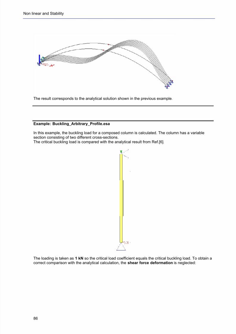
7/18/2019 Nonlinear and Stability 2013
http://slidepdf.com/reader/full/nonlinear-and-stability-2013 90/106
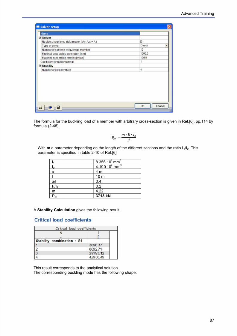
7/18/2019 Nonlinear and Stability 2013
http://slidepdf.com/reader/full/nonlinear-and-stability-2013 91/106
Advanced Training
87
The formula for the buckling load of a member with arbitrary cross-section is given in Ref.[6], pp.114 byformula (2-48):
EFG =H + I + JKL²
With m a parameter depending on the length of the different sections and the ratio I1/I2. This
parameter is specified in table 2-10 of Ref.[6].
I1 8.356 10 mm
I2 4.190 10 mm
a 4 m
l 10 ma/l 0.4
I1/I2 0.2
m 4.22
Pcr 3713 kN
A Stability Calculation gives the following result:
This result corresponds to the analytical solution.The corresponding buckling mode has the following shape:
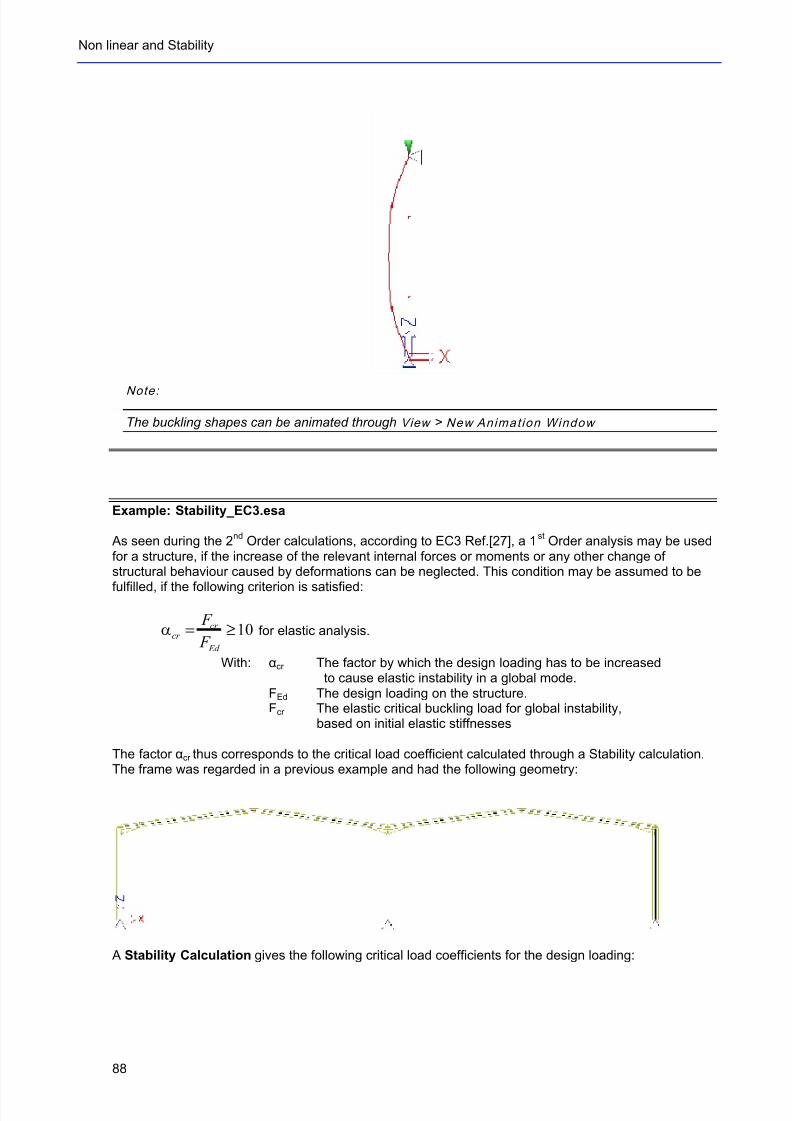
7/18/2019 Nonlinear and Stability 2013
http://slidepdf.com/reader/full/nonlinear-and-stability-2013 92/106
Non linear and Stability
88
Note:
The buckling shapes can be animated through View > New Animat ion Window
Example: Stability_EC3.esa
As seen during the 2nd
Order calculations, according to EC3 Ref.[27], a 1st Order analysis may be used
for a structure, if the increase of the relevant internal forces or moments or any other change ofstructural behaviour caused by deformations can be neglected. This condition may be assumed to be
fulfilled, if the following criterion is satisfied:
10≥= Ed
cr cr
F
F α for elastic analysis.
With: cr The factor by which the design loading has to be increasedto cause elastic instability in a global mode.
FEd The design loading on the structure.Fcr The elastic critical buckling load for global instability,
based on initial elastic stiffnesses
The factor cr thus corresponds to the critical load coefficient calculated through a Stability calculation.The frame was regarded in a previous example and had the following geometry:
A Stability Calculation gives the following critical load coefficients for the design loading:
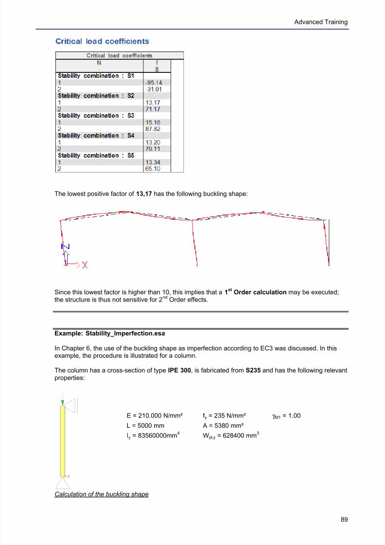
7/18/2019 Nonlinear and Stability 2013
http://slidepdf.com/reader/full/nonlinear-and-stability-2013 93/106
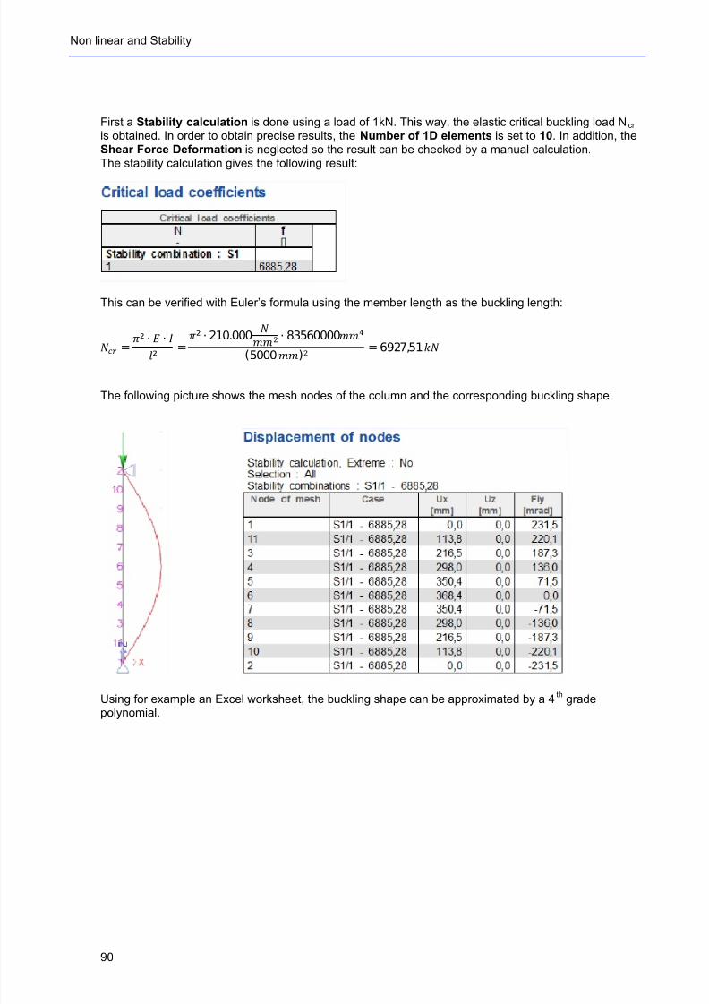
7/18/2019 Nonlinear and Stability 2013
http://slidepdf.com/reader/full/nonlinear-and-stability-2013 94/106
Non linear and Stability
90
First a Stability calculation is done using a load of 1kN. This way, the elastic critical buckling load Ncr is obtained. In order to obtain precise results, the Number of 1D elements is set to 10. In addition, theShear Force Deformation is neglected so the result can be checked by a manual calculation.The stability calculation gives the following result:
This can be verified with Euler’s formula using the member length as the buckling length:
MNO = P²
+ Q + RS² =T²
+210.000
UVWX +
83560000
YZ[
(5000 ]^)_ = 6927,51 ab
The following picture shows the mesh nodes of the column and the corresponding buckling shape:
Using for example an Excel worksheet, the buckling shape can be approximated by a 4
th
gradepolynomial.
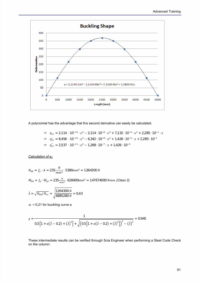
7/18/2019 Nonlinear and Stability 2013
http://slidepdf.com/reader/full/nonlinear-and-stability-2013 95/106
Advanced Training
91
A polynomial has the advantage that the second derivative can easily be calculated.
ð cde = 2,114 + 10fgh + ij O 2,114 + 10kl + mn + 7,132 + 10op + qr + 2,285 + 10st + u
ð vwxy = 8,456 + 10z{| + }~ O 6,342 + 10•! + "# + 1,426 + 10$% + & + 2,285+ 10'( ð
)*+" = 2,537
+10,-.
+ /0
O1,268
+1012
+ 3+ 1,426
+1045
Calculation of e0
678 = 9: + ; = 235<=>? + 5380@A² = 1264300 C
DEF = GH +IJK = 235 LMNO + 628400PQ³ = 147674000 STU (Class 2)
V W =
X YZ[/
\]^ =
_ 1264300 a6885280
c = 0,43
=α 0,21 for buckling curve a
d =1
0,5e1 +fgh WO 0.2i+jk Wlmn+o p0.5q1 +rst WO 0.2u+vw Wxyz{| O }~ W• = 0.945
These intermediate results can be verified through Scia Engineer when performing a Steel Code Checkon the column:
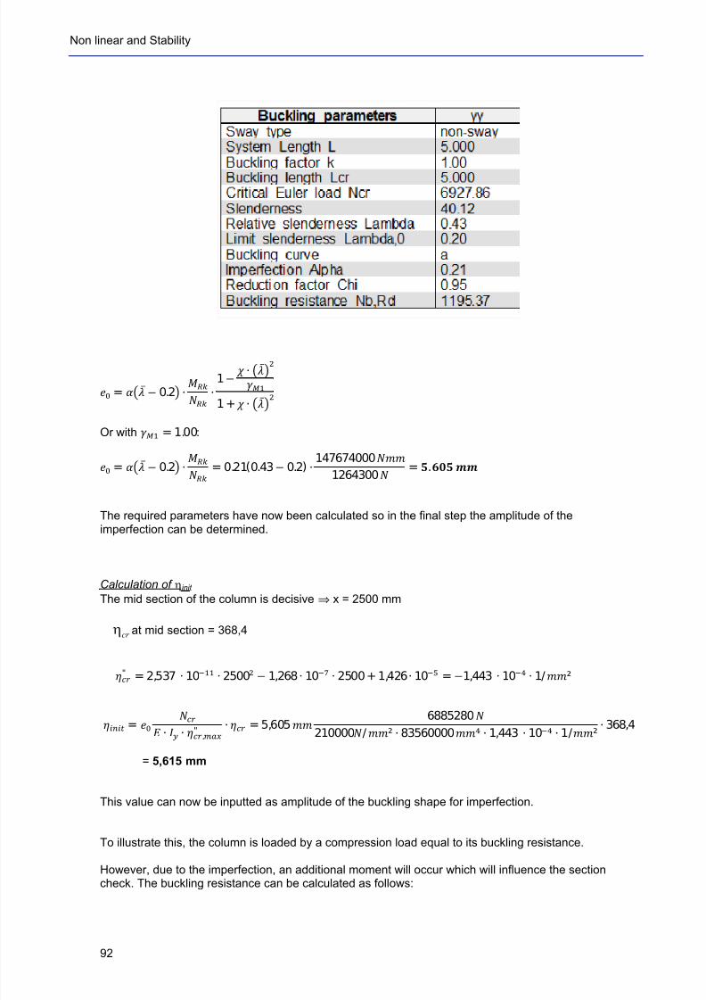
7/18/2019 Nonlinear and Stability 2013
http://slidepdf.com/reader/full/nonlinear-and-stability-2013 96/106
Non linear and Stability
92
!" = #$% WO 0.2& + '()
*+,+ 1 O - + ./ W01
2341 + 5 + 67 W89
Or with :;< = 1.00:
=> = ?@A WO 0.2B + CDE
FGH= 0.21(0.43 O 0.2) + 147674000 JKL
1264300 N = O.PQR TU
The required parameters have now been calculated so in the final step the amplitude of the
imperfection can be determined.
Calculation of ηinit
The mid section of the column is decisive ⇒ x = 2500 mm
cr η at mid section = 368,4
VWX" = 2,537 + 10YZ[ + 2500\ O 1,268 + 10]^ + 2500 + 1,426 + 10_` = O1,443 + 10ab + 1/cd²
efghi = jklmn
o + pq + rst,uvw"
+ xyz = 5,605 |} 6885280 •210000/!"² + 83560000 $%& + 1,443 + 10'( + 1/)*²
+ 368,4
= 5,615 mm
This value can now be inputted as amplitude of the buckling shape for imperfection.
To illustrate this, the column is loaded by a compression load equal to its buckling resistance.
However, due to the imperfection, an additional moment will occur which will influence the sectioncheck. The buckling resistance can be calculated as follows:
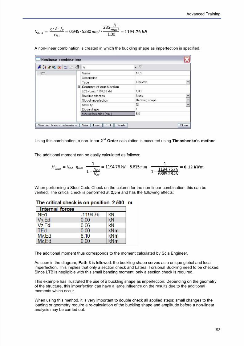
7/18/2019 Nonlinear and Stability 2013
http://slidepdf.com/reader/full/nonlinear-and-stability-2013 97/106
Advanced Training
93
+,,-. = / + 0 + 12345
= 0,945 + 5380 78² + 235 9:;<
1.00 ==>?@,AB DE
A non-linear combination is created in which the buckling shape as imperfection is specified.
Using this combination, a non-linear 2nd
Order calculation is executed using Timoshenko’s method.
The additional moment can be easily calculated as follows:
FGHIJK =LMN + OPQRS + 1
1 O TUVWXY
= 1194.76 [\ + 5.615 ^_ + 1
1 O 1194.76 ab6885.28 de
= f.gh jkl
When performing a Steel Code Check on the column for the non-linear combination, this can beverified. The critical check is performed at 2,5m and has the following effects:
The additional moment thus corresponds to the moment calculated by Scia Engineer.
As seen in the diagram, Path 3 is followed: the buckling shape serves as a unique global and localimperfection. This implies that only a section check and Lateral Torsional Buckling need to be checked.Since LTB is negligible with this small bending moment, only a section check is required.
This example has illustrated the use of a buckling shape as imperfection. Depending on the geometryof the structure, this imperfection can have a large influence on the results due to the additionalmoments which occur.
When using this method, it is very important to double check all applied steps: small changes to theloading or geometry require a re-calculation of the buckling shape and amplitude before a non-linearanalysis may be carried out.
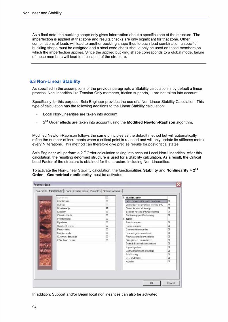
7/18/2019 Nonlinear and Stability 2013
http://slidepdf.com/reader/full/nonlinear-and-stability-2013 98/106
Non linear and Stability
94
As a final note: the buckling shape only gives information about a specific zone of the structure. Theimperfection is applied at that zone and results/checks are only significant for that zone. Othercombinations of loads will lead to another buckling shape thus to each load combination a specificbuckling shape must be assigned and a steel code check should only be used on those members onwhich the imperfection applies. Since the applied buckling shape corresponds to a global mode, failure
of these members will lead to a collapse of the structure.
6.3 Non-Linear Stability
As specified in the assumptions of the previous paragraph: a Stability calculation is by default a linearprocess. Non linearities like Tension-Only members, friction supports,… are not taken into account.
Specifically for this purpose, Scia Engineer provides the use of a Non-Linear Stability Calculation. Thistype of calculation has the following additions to the Linear Stability calculation:
- Local Non-Linearities are taken into account
- 2nd
Order effects are taken into account using the Modified Newton-Raphson algorithm.
Modified Newton-Raphson follows the same principles as the default method but will automaticallyrefine the number of increments when a critical point is reached and will only update its stiffness matrixevery N iterations. This method can therefore give precise results for post-critical states.
Scia Engineer will perform a 2nd
Order calculation taking into account Local Non-Linearities. After thiscalculation, the resulting deformed structure is used for a Stability calculation. As a result, the CriticalLoad Factor of the structure is obtained for the structure including Non-Linearities.
To activate the Non-Linear Stability calculation, the functionalities Stability and Nonlinearity > 2nd Order – Geometrical nonlinearity must be activated.
In addition, Support and/or Beam local nonlinearities can also be activated.
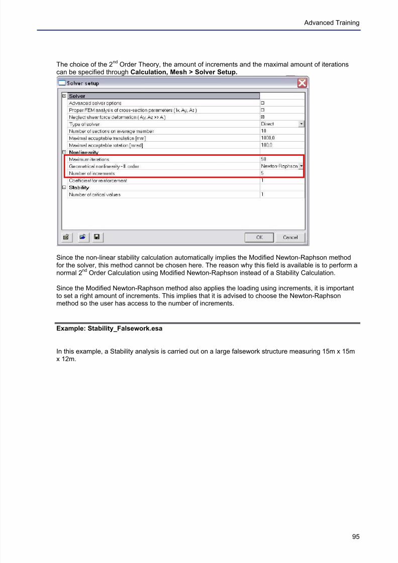
7/18/2019 Nonlinear and Stability 2013
http://slidepdf.com/reader/full/nonlinear-and-stability-2013 99/106
Advanced Training
95
The choice of the 2nd
Order Theory, the amount of increments and the maximal amount of iterationscan be specified through Calculation, Mesh > Solver Setup.
Since the non-linear stability calculation automatically implies the Modified Newton-Raphson methodfor the solver, this method cannot be chosen here. The reason why this field is available is to perform anormal 2
nd Order Calculation using Modified Newton-Raphson instead of a Stability Calculation.
Since the Modified Newton-Raphson method also applies the loading using increments, it is important
to set a right amount of increments. This implies that it is advised to choose the Newton-Raphsonmethod so the user has access to the number of increments.
Example: Stability_Falsework.esa
In this example, a Stability analysis is carried out on a large falsework structure measuring 15m x 15mx 12m.
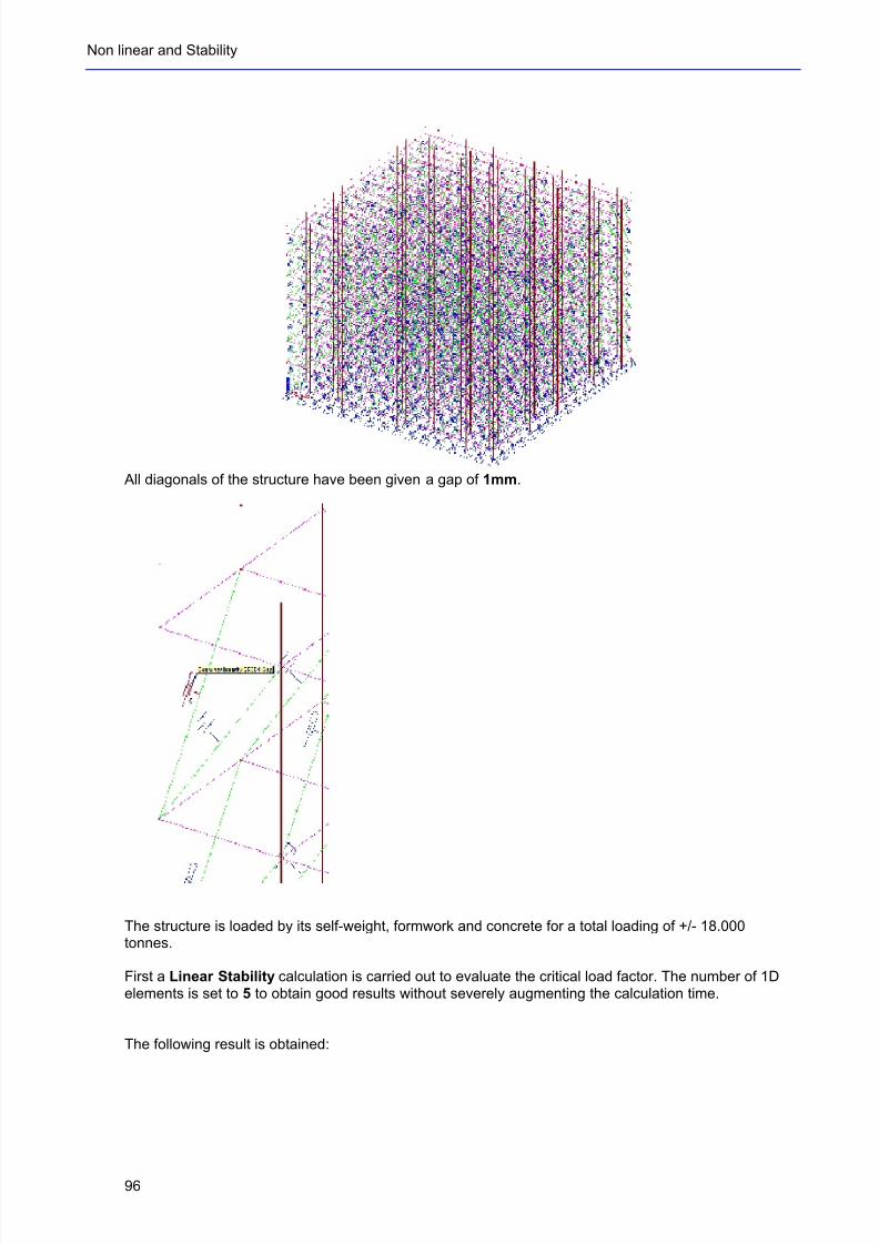
7/18/2019 Nonlinear and Stability 2013
http://slidepdf.com/reader/full/nonlinear-and-stability-2013 100/106
Non linear and Stability
96
All diagonals of the structure have been given a gap of 1mm.
The structure is loaded by its self-weight, formwork and concrete for a total loading of +/- 18.000tonnes.
First a Linear Stability calculation is carried out to evaluate the critical load factor. The number of 1Delements is set to 5 to obtain good results without severely augmenting the calculation time.
The following result is obtained:
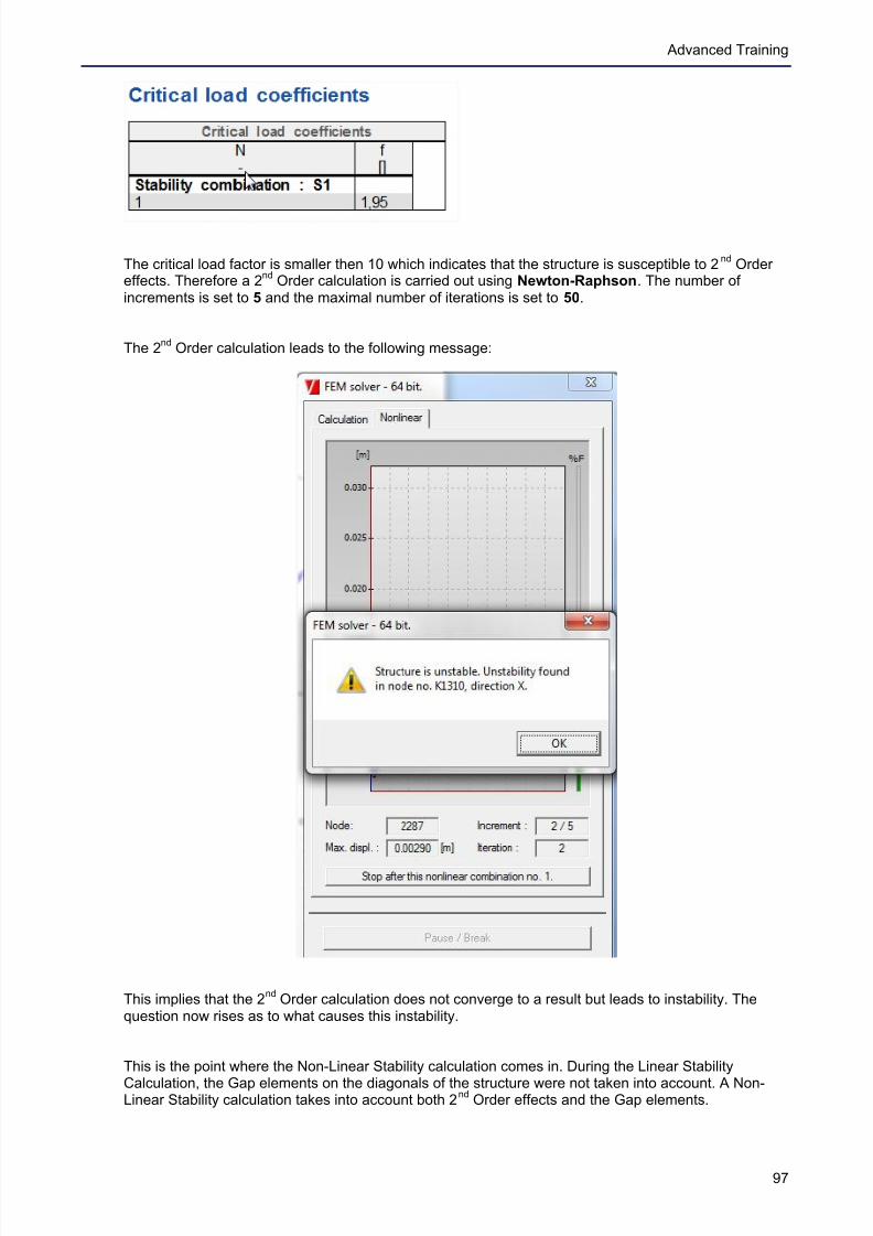
7/18/2019 Nonlinear and Stability 2013
http://slidepdf.com/reader/full/nonlinear-and-stability-2013 101/106
Advanced Training
97
The critical load factor is smaller then 10 which indicates that the structure is susceptible to 2nd
Ordereffects. Therefore a 2
nd Order calculation is carried out using Newton-Raphson. The number of
increments is set to 5 and the maximal number of iterations is set to 50.
The 2nd
Order calculation leads to the following message:
This implies that the 2nd
Order calculation does not converge to a result but leads to instability. Thequestion now rises as to what causes this instability.
This is the point where the Non-Linear Stability calculation comes in. During the Linear Stability
Calculation, the Gap elements on the diagonals of the structure were not taken into account. A Non-Linear Stability calculation takes into account both 2
nd Order effects and the Gap elements.

7/18/2019 Nonlinear and Stability 2013
http://slidepdf.com/reader/full/nonlinear-and-stability-2013 102/106
Non linear and Stability
98
The Non-Linear Stability Calculation gives the following result:
This result gives a very important conclusion: the structure including all Gap elements is not capable ofsupporting the loading. Only 26% of the loading can be supported before instability occurs. This is thereason why the 2
nd Order calculation does not pass.
When Local Non-Linearities are used, it is mandatory to execute a Non-Linear Stability calculation todraw correct conclusions concerning the global buckling of the structure.
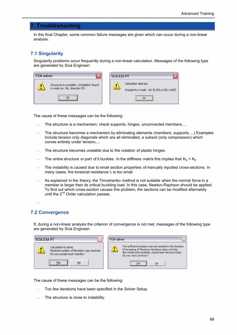
7/18/2019 Nonlinear and Stability 2013
http://slidepdf.com/reader/full/nonlinear-and-stability-2013 103/106
Advanced Training
99
7. Troubleshooting
In this final Chapter, some common failure messages are given which can occur during a non-linearanalysis.
7.1 Singularity
Singularity problems occur frequently during a non-linear calculation. Messages of the following typeare generated by Scia Engineer:
The cause of these messages can be the following:
- The structure is a mechanism: check supports, hinges, unconnected members,…
- The structure becomes a mechanism by eliminating elements (members, supports,…) Examplesinclude tension only diagonals which are all eliminated, a subsoil (only compression) whichcomes entirely under tension,…
- The structure becomes unstable due to the creation of plastic hinges.
- The entire structure or part of it buckles. In the stiffness matrix this implies that KG > KE
- The instability is caused due to small section properties of manually inputted cross-sections. Inmany cases, the torsional resistance It is too small.
- As explained in the theory, the Timoshenko method is not suitable when the normal force in amember is larger then its critical buckling load. In this case, Newton-Raphson should be applied.To find out which cross-section causes this problem, the sections can be modified alternatelyuntil the 2
nd Order calculation passes.
-
7.2 Convergence
If, during a non-linear analysis the criterion of convergence is not met, messages of the following typeare generated by Scia Engineer:
The cause of these messages can be the following:
- Too few iterations have been specified in the Solver Setup.
- The structure is close to instability.

7/18/2019 Nonlinear and Stability 2013
http://slidepdf.com/reader/full/nonlinear-and-stability-2013 104/106
Non linear and Stability
100
- Cyclic elimination of members or supports: the elements are eliminated during an iteration andare re-instated during the following iteration.
- To examine this in detail, the calculation can be executed for for example three iterations: take
iteration i-1, i and i+1 and compare the results.
In these results, there will be a difference in one member (for example in one iteration themember is in tension, in the following iteration it is in compression).
- If the non-linear stability calculation does not converge, make sure 2nd
Order is activated asfunctionality.
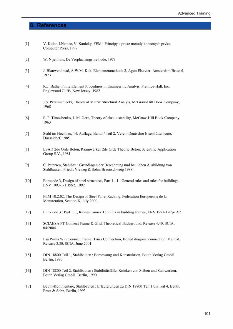
7/18/2019 Nonlinear and Stability 2013
http://slidepdf.com/reader/full/nonlinear-and-stability-2013 105/106
Advanced Training
101
8. References
[1] V. Kolar, I.Nemec, V. Kanicky, FEM : Principy a praxe metody konecnych prvku,
Computer Press, 1997
[2] W. Nijenhuis, De Verplaatsingsmethode, 1973
[3] J. Blauwendraad, A.W.M. Kok, Elementenmethode 2, Agon Elsevier, Amsterdam/Brussel,
1973
[4] K.J. Bathe, Finite Element Procedures in Engineering Analyis, Prentice-Hall, Inc.
Englewood Cliffs, New Jersey, 1982
[5] J.S. Przemieniecki, Theory of Matrix Structural Analyis, McGraw-Hill Book Company,
1968
[6] S. P. Timoshenko, J. M. Gere, Theory of elastic stability, McGraw-Hill Book Company,
1963
[7] Stahl im Hochbau, 14. Auflage, BandI / Teil 2, Verein Deutscher Eisenhüttenleute,
Düsseldorf, 1985
[8] ESA 3 2de Orde Beton, Raamwerken 2de Orde Theorie Beton, Scientific Application
Group S.V., 1981
[9] C. Petersen, Stahlbau : Grundlagen der Berechnung und baulichen Ausbildung von
Stahlbauten, Friedr. Vieweg & Sohn, Braunschweig 1988
[10] Eurocode 3, Design of steel structures, Part 1 - 1 : General rules and rules for buildings,
ENV 1993-1-1:1992, 1992
[11] FEM 10.2.02, The Design of Steel Pallet Racking, Fédération Européenne de la
Manutention, Section X, July 2000
[12] Eurocode 3 : Part 1.1., Revised annex J : Joints in building frames, ENV 1993-1-1/pr A2
[13] SCIAESA PT Connect Frame & Grid, Theoretical Background, Release 4.40, SCIA,
04/2004
[14] Esa Prima Win Connect Frame, Truss Connection, Bolted diagonal connection, Manual,Release 3.30, SCIA, June 2001
[15] DIN 18800 Teil 1, Stahlbauten : Bemessung und Konstruktion, Beuth Verlag GmbH,
Berlin, 1990
[16] DIN 18800 Teil 2, Stahlbauten : Stabilitätsfälle, Knicken von Stäben und Stabwerken,Beuth Verlag GmbH, Berlin, 1990
[17] Beuth-Kommentare, Stahlbauten : Erläuterungen zu DIN 18800 Teil 1 bis Teil 4, Beuth,Ernst & Sohn, Berlin, 1993
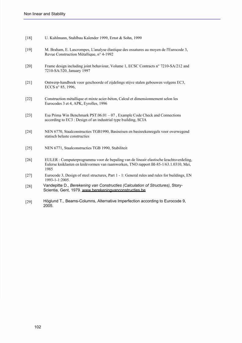
7/18/2019 Nonlinear and Stability 2013
http://slidepdf.com/reader/full/nonlinear-and-stability-2013 106/106
Non linear and Stability
[18] U. Kuhlmann, Stahlbau Kalender 1999, Ernst & Sohn, 1999
[19] M. Braham, E. Lascrompes, L'analyse élastique des ossatures au moyen de l'Eurocode 3,
Revue Construction Métallique, n° 4-1992
[20] Frame design including joint behaviour, Volume 1, ECSC Contracts n° 7210-SA/212 and
7210-SA/320, January 1997
[21] Ontwerp-handboek voor geschoorde of zijdelings stijve stalen gebouwen volgens EC3,ECCS n° 85, 1996,
[22] Construction métallique et mixte acier-béton, Calcul et dimensionnement selon les
Eurocodes 3 et 4, APK, Eyrolles, 1996
[23] Esa Prima Win Benchmark PST.06.01 – 07 , Example Code Check and Connections
according to EC3 : Design of an industrial type building, SCIA
[24] NEN 6770, Staalconstructies TGB1990, Basiseisen en basisrekenregels voor overwegend
statisch belaste constructies
[25] NEN 6771, Staalconstructies TGB 1990, Stabiliteit
[26] EULER : Computerprogramma voor de bepaling van de lineair elastische krachtsverdeling,Eulerse kniklasten en knikvormen van raamwerken, TNO rapport BI-85-1/63.1.0310, Mei,
1985
[27] Eurocode 3, Design of steel structures, Part 1 - 1: General rules and rules for buildings, EN
1993-1-1:2005.[28] Vandepitte D., Berekening van Constructies (Calculation of Structures), Story-
Scientia, Gent, 1979. www.berekeningvanconstructies.be
[29] Höglund T., Beams-Columns, Alternative Imperfection according to Eurocode 9,2005.