Nonlinear Blind Source Separation byIntegrating Independent Component Analysis

and Slow Feature Analysis

Tobias BlaschkeInstitute for Theoretical Biology

Humboldt University BerlinInvalidenstraße 43, D-10115 Berlin, Germanyt.blaschke@biologie.hu-berlin.de

Laurenz WiskottInstitute for Theoretical Biology

Humboldt University BerlinInvalidenstraße 43, D-10115 Berlin, Germanyl.wiskott@biologie.hu-berlin.de

Abstract

In contrast to the equivalence of linear blind source separation and linearindependent component analysis it is not possible to recover the origi-nal source signal from some unknown nonlinear transformations of thesources using only the independence assumption. Integrating the ob-jectives of statistical independence and temporal slowness removes thisindeterminacy leading to a new method for nonlinear blind source sepa-ration. The principle of temporal slowness is adopted from slow featureanalysis, an unsupervised method to extract slowly varying features froma given observed vectorial signal. The performance of the algorithm isdemonstrated on nonlinearly mixed speech data.

1 Introduction

Unlike in the linear case the nonlinear Blind Source Separation (BSS) problem can not besolved solely based on the principle of statistical independence [1, 2]. Performing non-linear BSS with Independent Component Analysis (ICA) requires additional informationabout the underlying sources or to regularize the nonlinearities. Since source signal com-ponents are usually more slowly varying than any nonlinear mixture of them we considerto require the estimated sources to be as slowly varying as possible. This can be achievedby incorporating ideas from Slow Feature Analysis (SFA) [3] into ICA.

After a short introduction to linear BSS, nonlinear BSS, and SFA we will show a way howto combine SFA and ICA to obtain an algorithm that solves the nonlinear BSS problem.

2 Linear Blind Source Separation

Let x(t) = [x1 (t) , . . . , xN (t)]T be a linear mixture of a source signal s(t) =

[s1 (t) , . . . , sN (t)]T and defined by

x (t) = As (t) , (1)

with an invertible N × N mixing matrix A. Finding a mapping

u (t) = QWx (t) (2)

such that the components of u are mutually statistically independent is called Indepen-dent Component Analysis (ICA). The mapping is often divided into a whitening mappingW, resulting in uncorrelated signal components yi with unit variance and a successive or-thogonal transformation Q, because one can show [4] that after whitening an orthogonaltransformation is sufficient to obtain independence. It is well known that ICA solves thelinear BSS problem [4]. There exists a variety of algorithms performing ICA and thereforeBSS (see e.g. [5, 6, 7]). Here we focus on a method using only second-order statisticsintroduced by Molgedey and Schuster [8]. The method consists of optimizing an objectivefunction subject to minimization, which can be written as

ΨICA (Q) =N

∑

α,β=1

α6=β

(

C(u)αβ (τ)

)2

=N

∑

α,β=1

α6=β

N∑

γ,δ=1

QαγQβδC(y)γδ (τ)

2

, (3)

operating on the already whitened signal y. C(y)γδ (τ) is an entry of a symmetrized time

delayed covariance matrix defined by

C(y) (τ) =⟨

y (t)y (t + τ)T

+ y (t + τ)y (t)T⟩

, (4)

and C(u) (τ) is defined correspondingly. Qαβ denotes an entry of Q. Minimization ofΨICA can be understood intuitively as finding an orthogonal matrix Q that diagonalizes thecovariance matrix with time delay τ . Since, because of the whitening, the instantaneouscovariance matrix is already diagonal this results in signal components that are decorrelatedinstantaneously and at a given time delay τ . This can be sufficient to achieve statisticalindependence [9].

2.1 Nonlinear BSS and ICA

An obvious extension to the linear mixing model (1) has the form

x (t) = F (s (t)) , (5)

with a function F (· ) RN → R

M that maps N -dimensional source vectors s onto M -dimensional signal vectors x. The components xi of the observable are a nonlinear mixtureof the sources and like in the linear case source signal components si are assumed to bemutually statistically independent. Extracting the source signal is in general only possibleif F (· ) is an invertible function, which we will assume from now on.

The equivalence of BSS and ICA in the linear case does in general not hold for a nonlinearfunction F (· ) [1, 2]. To solve the nonlinear BSS problem additional constraints on themixture or the estimated signals are needed to bridge the gap between ICA and BSS. Herewe propose a new way to achieve this by adding a slowness objective to the independenceobjective of pure ICA. Assume for example a sinusoidal signal component xi = sin (2πt)and a second component that is the square of the first xj = x2

i = 0.5 (1 − cos (4πt))is given. The second component is more quickly varying due to the frequency doubling

induced by the squaring. Typically nonlinear mixtures of signal components are morequickly varying than the original components. To extract the right source components oneshould therefore prefer the slowly varying ones. The concept of slowness is used in ourapproach to nonlinear BSS by combining an ICA part that provides the independence ofthe estimated source signal components with a part that prefers slowly varying signals overmore quickly varying ones. In the next section we will give a short introduction to SlowFeature Analysis (SFA) building the basis of the second part of our method.

3 Slow Feature Analysis

Assume a vectorial input signal x(t) = [x1(t), . . . , xM (t)]T is given. The objective of SFA

is to find an in general nonlinear input-output function u (t) = g (x (t)) with g (x (t)) =

[g1 (x (t)) , . . . , gR (x (t))]T such that the ui (t) are varying as slowly as possible. This

can be achieved by successively minimizing the objective function

∆(ui) :=⟨

u2i

⟩

(6)

for each ui under the constraints

〈ui〉 = 0 (zero mean), (7)⟨

u2i

⟩

= 1 (unit variance), (8)

〈uiuj〉 = 0 ∀ j < i (decorrelation and order). (9)

Constraints (7) and (8) ensure that the solution will not be the trivial solution ui = const.Constraint (9) provides uncorrelated output signal components and thus guarantees thatdifferent components carry different information. Intuitively we are searching for signalcomponents ui that have on average a small slope.

Interestingly Slow Feature Analysis (SFA) can be reformulated with an objective functionsimilar to second-order ICA, subject to maximization [10],

ΨSFA (Q) =

M∑

α=1

(

C(u)αα (τ)

)2

=

M∑

α=1

M∑

β,γ=1

QαβQαγC(y)βγ (τ)

2

. (10)

To understand (10) intuitively we notice that slowly varying signal components are easierto predict, and should therefore have strong auto correlations in time. Thus, maximizingthe time delayed variances produces slowly varying signal components.

4 Independent Slow Feature Analysis

If we combine ICA and SFA we obtain a method we refer to as Independent Slow FeatureAnalysis (ISFA) that recovers independent components out of a nonlinear mixture using acombination of SFA and second-order ICA. As already explained, second-order ICA tendsto make the output components independent and SFA tends to make them slow. Sincewe are dealing with a nonlinear mixture we first compute a nonlinearly expanded signalz = h (x) with h (· ) R

M → RL being typically monomials up to a given degree, e.g. an

expansion with monomials up to second degree can be written as

h (x (t)) = [x1, . . . , xN , x1x1, x1x2, . . . , xMxM ]T− hT

0 (11)

when given an M -dimensional signal x. The constant vector hT0 is used to make the ex-

panded signal mean free. In a second step z is whitened to obtain y = Wz. Thirdly weapply linear ICA combined with linear SFA on y in order to find the estimated source signal

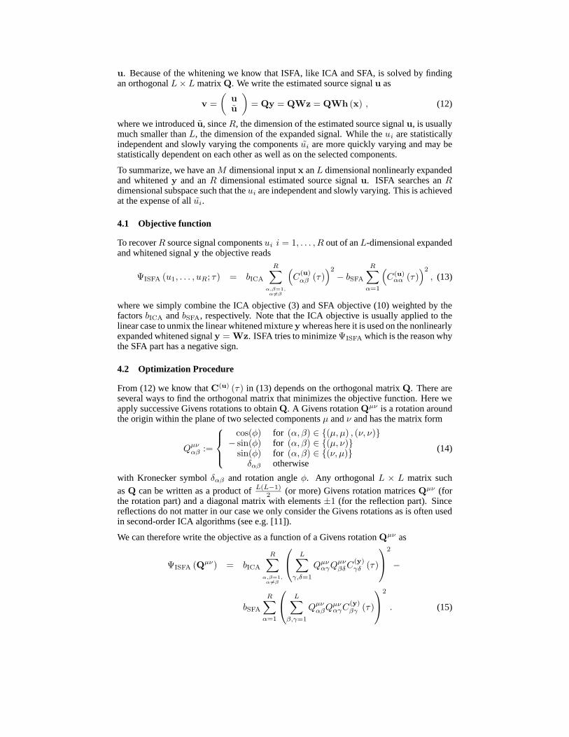
u. Because of the whitening we know that ISFA, like ICA and SFA, is solved by findingan orthogonal L × L matrix Q. We write the estimated source signal u as

v =

(

uu

)

= Qy = QWz = QWh (x) , (12)

where we introduced u, since R, the dimension of the estimated source signal u, is usuallymuch smaller than L, the dimension of the expanded signal. While the ui are statisticallyindependent and slowly varying the components ui are more quickly varying and may bestatistically dependent on each other as well as on the selected components.

To summarize, we have an M dimensional input x an L dimensional nonlinearly expandedand whitened y and an R dimensional estimated source signal u. ISFA searches an Rdimensional subspace such that the ui are independent and slowly varying. This is achievedat the expense of all ui.

4.1 Objective function

To recover R source signal components ui i = 1, . . . , R out of an L-dimensional expandedand whitened signal y the objective reads

ΨISFA (u1, . . . , uR; τ) = bICA

R∑

α,β=1,α6=β

(

C(u)αβ (τ)

)2

− bSFA

R∑

α=1

(

C(u)αα (τ)

)2

, (13)

where we simply combine the ICA objective (3) and SFA objective (10) weighted by thefactors bICA and bSFA, respectively. Note that the ICA objective is usually applied to thelinear case to unmix the linear whitened mixture y whereas here it is used on the nonlinearlyexpanded whitened signal y = Wz. ISFA tries to minimize ΨISFA which is the reason whythe SFA part has a negative sign.

4.2 Optimization Procedure

From (12) we know that C(u) (τ) in (13) depends on the orthogonal matrix Q. There areseveral ways to find the orthogonal matrix that minimizes the objective function. Here weapply successive Givens rotations to obtain Q. A Givens rotation Qµν is a rotation aroundthe origin within the plane of two selected components µ and ν and has the matrix form

Qµναβ :=

cos(φ) for (α, β) ∈ {(µ, µ) , (ν, ν)}− sin(φ) for (α, β) ∈ {(µ, ν)}

sin(φ) for (α, β) ∈ {(ν, µ)}δαβ otherwise

(14)

with Kronecker symbol δαβ and rotation angle φ. Any orthogonal L × L matrix such

as Q can be written as a product of L(L−1)2 (or more) Givens rotation matrices Qµν (for

the rotation part) and a diagonal matrix with elements ±1 (for the reflection part). Sincereflections do not matter in our case we only consider the Givens rotations as is often usedin second-order ICA algorithms (see e.g. [11]).

We can therefore write the objective as a function of a Givens rotation Qµν as

ΨISFA (Qµν) = bICA

R∑

α,β=1,α6=β

L∑

γ,δ=1

QµναγQµν

βδC(y)γδ (τ)

2

−

bSFA

R∑

α=1

L∑

β,γ=1

QµναβQµν

αγC(y)βγ (τ)

2

. (15)

Assume we want to minimize ΨISFA for a given R, where R denotes the number of signalcomponents we want to extract. Applying a Givens rotation Qµν we have to distinguishthree cases.

• Case 1: Both axes uµ and uν lie inside the subspace spanned by the first R axes(µ, ν ≤ R). The sum over all squared cross correlations of all signal componentsthat lie outside the subspace is constant as well as those of all signal componentsinside the subspace. There is no interaction between inside and outside, in fact theobjective function is exactly the objective for an ICA algorithm based on second-order statistics e.g. TDSEP or SOBI [12, 13]. In [10] it has been shown that thisis equivalent to SFA in the case of a single time delay.

• Case 2: Only one axis, w.l.o.g. uµ, lies inside the subspace, the other, uν , outside(µ ≤ R < ν). Since one axis of the rotation plane lies outside the subspace, uµ inthe objective function can be optimized at the expense of uν outside the subspace.A rotation of π/2, for instance, would simply exchange components uµ and uν .This gives the possibility to find the slowest and most independent components inthe whole space spanned by all ui and uj (i = 1, . . . , R, j = R + 1, . . . , L) incontrast to Case 1 where the minimum is searched within the subspace spannedby the R components in the objective function.

• Case 3: Both axes lie outside the subspace (R < µ, ν): A Givens rotation withthe two rotation axes outside the relevant subspace does not affect the objectivefunction and can therefore be disregarded.

It can be shown that like in [14] the objective function (15) as a function of φ can alwaysbe written in the form

ΨµνISFA (φ) = A0 + A2 cos (2φ + φ2) + A4 cos (4φ + φ4) , (16)

where the second term on the right hand side vanishes for Case 1. There exists a singleminimum (if w.l.o.g. φ ∈

[

−π2 , π

2

]

) that can easily be calculated (see e.g.[14]). Thederivation of (16) involves various trigonometric identities and, because of its length, isdocumented elsewhere1.

It is important to notice that the rotation planes of the Givens rotations are selected fromthe whole L-dimensional space whereas the objective function only uses information ofcorrelations among the first R signal components ui. Successive application of Givensrotations Qµν leads to the final rotation matrix Q which is in the ideal case such thatQT C(y) (τ)Q = C(v) (τ) has a diagonal R × R submatrix C(u) (τ), but it is not clear ifthe final minimum is also the global one. However, in various simulations no local minimahave been found.

4.3 Incremental Extracting of Independent Components

It is possible to find the number of independent source signal components R by succes-sively increasing the number of components to be extracted. In each step the objectivefunction (13) is optimized for a fixed R. First a single signal component is extracted(R = 1) and then an additional one (R = 2) etc. The algorithm is stopped when no addi-tional signal component can be extracted. As a stopping criterion every suitable measureof independence can be applied; we used the sum over squared cross-cumulants of fourthorder. In our artificial examples this value is typically small for independent components,and increases by two orders of magnitudes if the number of components to be extracted isgreater than the number of original source signal components.

1http://itb.biologie.hu-berlin.de/~blaschke

5 Simulation

Here we show a simple example, with two nonlinearly mixed signal components as shownin Figure 1. The mixture is defined by

x1 (t) = (s1 (t) + 1) sin (πs2 (t)) ,

x2 (t) = (s1 (t) + 1) cos (πs2 (t)) . (17)

We used the ISFA algorithm with different nonlinearities (see Tab. 1). Already a nonlin-ear expansion with monomials up to degree three was sufficient to give good results inextracting the original source signal (see Fig. 1). In all cases ISFA did find exactly twoindependent signal components. A linear BSS method failed completely to find a goodunmixing matrix.

6 Conclusion

We have shown that connecting the ideas of slow feature analysis and independent com-ponent analysis into ISFA is a possible way to solve the nonlinear blind source separationproblem. SFA enforces the independent components of ICA to be slowly varying whichseems to be a good way to discriminate between the original and nonlinearly distortedsource signal components. A simple simulation showed that ISFA is able to extract theoriginal source signal out of a nonlinear mixture. Furthermore ISFA can predict the num-ber of source signal components via an incremental optimization scheme.

Acknowledgments

This work has been supported by the Volkswagen Foundation through a grant to LW for ajunior research group.

References

[1] A. Hyvärinen and P. Pajunen. Nonlinear independent component analysis: existenceand uniqueness results. Neural Networks, 12(3):429–439, 1999.

[2] C. Jutten and J. Karhunen. Advances in nonlinear blind source separation. In Proc.of the 4th Int. Symposium on Independent Component Analysis and Blind Signal Sep-aration, Nara, Japan, (ICA 2003), pages 245–256, 2003.

[3] Laurenz Wiskott and Terrence Sejnowski. Slow feature analysis: Unsupervised learn-ing of invariances. Neural Computation, 14(4):715–770, 2002.

Table 1: Correlation coefficients of extracted (u1 and u2) and original (s1 and s2) sourcesignal components

linear degree 2 degree 3 degree 4u1 u2 u1 u2 u1 u2 u1 u2

s1 -0.803 -0.544 -0.001 -0.978 0.001 0.995 0.002 0.995s2 0.332 0.517 -0.988 -0.001 -0.995 0.001 -0.996 0.000

Correlation coefficients of extracted (u1 and u2) and original (s1 and s2) source signal com-ponents for linear ICA (first column) and ISFA with different nonlinearities (monomials upto degree 2, 3, and 4). Using monomials up to degree 3 in the nonlinear expansion stepalready suffices to extract the original source signal. Note that the source signal can onlybe estimated up to permutation and scaling, resulting in different signs and permutations ofthe two estimated source signal components.

s1

s2

(a)

x1

x2

(b)

u1

u2

(c)

Figure 1: Waveforms and Scatter-plots of (a) the original source signal components si,(b) the nonlinear mixture, and (c) recovered components with nonlinear ISFA (ui). As anonlinearity we used all monomials up to degree 4.

[4] P. Comon. Independent component analysis, a new concept? Signal Processing,36(3):287–314, 1994. Special Issue on Higher-Order Statistics.

[5] J.-F. Cardoso and A. Souloumiac. Blind beamforming for non Gaussian signals. IEEProceedings-F, 140:362–370, 1993.

[6] T.-W. Lee, M. Girolami, and T.J. Sejnowski. Independent component analysis usingan extended Infomax algorithm for mixed sub-Gaussian and super-Gaussian sources.Neural Computation, 11(2):409–433, 1999.

[7] A. Hyvärinen. Fast and robust fixed-point algorithms for independent componentanalysis. IEEE Transactions on Neural Networks, 10(3):626–634, 1999.

[8] L. Molgedey and G. Schuster. Separation of a mixture of independent signals usingtime delayed correlations. Physical Review Letters, 72(23):3634–3637, 1994.

[9] Lang Tong, Ruey-wen Liu, Victor C. Soon, and Yih-Fang Huang. Indeterminacy andidentifiability of blind identification. IEEE Transactions on Circuits and Systems,38(5):499–509, may 1991.

[10] T. Blaschke, L. Wiskott, and P. Berkes. What is the relation between independentcomponent analysis and slow feature analysis? (in preparation), 2004.

[11] Jean-François Cardoso and Antoine Souloumiac. Jacobi angles for simultaneous di-agonalization. SIAM J. Mat. Anal. Appl., 17(1):161–164, 1996.

[12] A. Ziehe and K.-R. Müller. TDSEP – an efficient algorithm for blind separation usingtime structure. In Proc. of the 8th Int. Conference on Artificial Neural Networks(ICANN’98), pages 675 – 680, Berlin, 1998. Springer Verlag.

[13] Adel Belouchrani, Karim Abed Meraim, Jean-François Cardoso, and Éric Moulines.A blind source separation technique based on second order statistics. IEEE Transac-tions on Signal Processing, 45(2):434–44, 1997.

[14] T. Blaschke and L. Wiskott. CuBICA: Independent component analysis by simulta-neous third- and fourth-order cumulant diagonalization. IEEE Transactions on SignalProcessing, 52(5):1250–1256, 2004.