Embed Size (px)
Citation preview
Nonlinear Controller Design for Input-Constrained, MultivariableProcesses
Joshua M. Kanter,† Masoud Soroush,*,‡ and Warren D. Seider†
Department of Chemical Engineering, University of Pennsylvania, Philadelphia, Pennsylvania 19104-6393and Department of Chemical Engineering, Drexel University, Philadelphia, Pennsylvania 19104
Nonlinear control laws are presented for input-constrained, multiple-input, multiple-outputprocesses, whether their delay-free part is minimum or nonminimum phase. This study addressesthe nonlinear control of input-constrained processes by exploiting the connections between model-predictive control and input-output linearization. The continuous-time control laws involve thesolution of constrained optimization problems online. They minimize the error between controlledoutputs and their reference trajectories, subject to the input constraints. Their application andperformance are illustrated using numerical simulation of two chemical reactors that exhibitnonminimum-phase behavior.
1. Introduction
Over the past 20 years, significant advances havebeen made in nonlinear model-based control. Theseadvances have been mainly in the frameworks of model-predictive control (MPC) and differential geometriccontrol. In model-predictive control, input constraintsare explicitly accounted for, and the controller action isthe solution of a constrained optimization problem.Differential geometric control, in contrast, is a directsynthesis approach in which a controller is derived byrequesting a desired unconstrained response.
While in model-predictive control nonminimum-phasebehavior is handled simply by using larger predictionhorizons, in differential geometric control special treat-ment is necessary. In the latter, advances first madefor unconstrained, minimum-phase (MP) processes havebeen extended to unconstrained nonminimum-phase(NMP) processes.3-16 Those based on factorization ofthe process model3,4 and equivalent outputs5,6 arelimited to single-input single-output, NMP processes.Others are applicable to multiinput multioutput (MIMO)processes, whether MP or NMP.7,8-15 However, eithersets of partial differential equations must besolved8-10 or the process is subject to restrictions.11-15
Furthermore, input constraints and deadtimes are notconsidered during controller design for these MIMOprocesses.
The main objective of this work is to derive nonlinearcontrol laws for input-constrained, MIMO, stable, non-linear processes with a nonminimum-phase or minimum-phase delay-free part. Continuous-time, differentialgeometric control laws are derived that are approxi-mately input-output linearizing in the absence of inputconstraints. The connections between these optimiza-tion-based controllers and those derived using a directsynthesis approach16 are established.
This paper is organized as follows. The scope of thestudy and some mathematical preliminaries are given
in section 2. Section 3 introduces a method of nonlinearfeedforward/state feedback design for input-constrainedprocesses. Methods of designing nonlinear feedbackcontrollers with integral action in the presence of inputconstraints are given in section 4. Finally, the applica-tion and performance of the control laws are illustratedby numerical simulation of two chemical reactors insection 5.
2. Scope and Mathematical Preliminaries
Consider the class of MIMO, nonlinear processes ofthe form
where xj ) [xj1...xjn]T ∈ X is the vector of the process statevariables, u ) [u1...um]T ∈ U is the vector of manip-ulated inputs, yj ) [yj1...yjm]T is the vector of processoutputs, θ1, ..., θm are the measurement delays, d )[d1...dm]T ∈ D is the vector of constant unmeasureddisturbances, f (‚,‚) is a smooth vector field on X × U,and h1(‚), ..., hm(‚) are smooth functions on X. HereX ⊂ Rn is a connected open set that includes xjss andxj0; U ) {u|uli e ui e uhi, i ) 1, ..., m} ⊂ Rm that in-cludes uss; ul1, ..., ulm, uh1, ..., uhm are real scalars; D ⊂Rm is a connected set; and (xjss, uss) denotes the nominalsteady-state (equilibrium) pair of the process; that is,f[xjss,uss] ) 0.
The system
is referred to as the delay-free part of the process. Therelative orders (degrees) of the controlled outputs yj1, ...,yjm with respect to u are denoted by r1, ..., rm, respec-tively, where ri is the smallest integer for which driyji
//dtri
* Corresponding author. Telephone (215) 895-1710. Fax:(215) 895-5837. E-mail: [email protected].
† University of Pennsylvania.‡ Drexel University.
dxj(t)dt
) f[xj(t),u(t)], xj(0) ) xj0
yji(t) ) hi[xj(t - θi)] + di
ulie ui(t) e uhi
, i ) 1, ..., m } (1)
dxj(t)dt
) f[xj(t),u(t)], xj(0) ) xj0
yji/(t) ) hi[xj(t)] + di
ulie ui(t) e uhi
, i ) 1, ..., m } (2)
3735Ind. Eng. Chem. Res. 2002, 41, 3735-3744
10.1021/ie0105066 CCC: $22.00 © 2002 American Chemical SocietyPublished on Web 11/27/2001
explicitly depends on u for every x ∈ X and every u ∈ U.The set point and the set of acceptable set point valuesare denoted by ysp and Y, respectively, where Y ⊂ Rm isa connected set.
The following assumptions are made:(A1) For every ysp ∈ Y and every d ∈ D, there exists
an equilibrium pair (xjss, uss) ∈ X × U that satisfies ysp- d ) h(xjss) and f[xjss, uss] ) 0.
(A2) The nominal steady-state (equilibrium) pair ofthe process, (xjss, uss), is hyperbolically stable; that is,all eigenvalues of the Jacobian of the open-loop processevaluated at (xjss, uss) have negative real parts.
(A3) For a process in the form of (1), a model in thefollowing form is available:
where x ) [x1...xn]T ∈ X is the vector of model statevariables, and y ) [y1, ..., ym]T is the vector of modeloutputs.
(A4) The relative orders, r1, ..., rm, are finite.The following notation is used:
where pi g ri and u(l) ) dlu/dtl.2.1. Unconstrained Feedback Controller Design
via Direct Synthesis: Review. Consider the followingnotation:
where ε1, ..., εm are positive, adjustable, constant scalars
Assume that for every x ∈ X, every d ∈ D, and everyysp ∈ Y, the algebraic equation
where
has a real root for u, and that for every xj ∈ X and everyu ∈ R m, ∂φp(xj,u)/∂u is nonsingular. The correspondingfeedforward/state feedback that satisfies eq 6 is denotedby
Theorem 1.16 For a process in the form of eq 1without input constraints and with state measurementsxj and θ1 ) ... ) θm ) 0, the closed-loop system underthe mixed error- and state-feedback control law
is asymptotically stable, if the following conditions hold:(a) The nominal equilibrium pair of the process,
(xjss,uss), corresponding to ysp and d, is hyperbolicallystable.
(b) The tunable parameters p1, ..., pm are chosen tobe sufficiently large.
(c) The tunable parameters ε1, ..., εm are chosen suchthat, for every l ) 1, ..., m, all eigenvalues of εl Jol }εl[∂/∂x f(x,u)](xjss,uss) lie inside the unit circle centered at(-1, 0j).Furthermore, the mixed error- and state-feedback con-trol law of eq 9 has integral action. Here Ac ) block-diag(Ac1, ..., Acm), Bc ) block-diag(Bc1, ..., Bcm), and Cc )block-diag(Cc1, ..., Ccm) are (p1 + ... + pm) × (p1 + ... +pm), (p1 + ... + pm) × m, and m × (p1 + ... + pm) blockdiagonal, constant matrices, respectively. A typicalmatrix triplet (Aci, Bci, Cci) is
dx(t)dt
) f[x(t),u(t)], x(0) ) x0
yi(t) ) hi[x(t - θi)]uli
e ui(t) e uhi, i ) 1, ‚‚‚, m } (3)
hi1(x) } [∂hi(x)
∂x ]f(x,u) )dyi
/
dt
l
hiri-1(x) } [∂hi
ri-2(x)∂x ]f(x,u) )
dri-1yi/
dtri-1
hiri(x,u) } [∂hi
ri-1(x)∂x ]f(x,u) )
driyi/
dtri
hiri+1(x,u(0),u(1)) } [∂hi
ri(x,u)∂x ]f(x,u) +
[∂hiri(x,u)∂u ]u(1) )
dri+1yi/
dtri+1
l
hipi(x,u(0),u(1),...,u(pi-ri)) }
[∂hipi-1(x,u(0),...,u(pi-ri-1))
∂x ]f(x,u) +
[∂hipi-1(x,u(0),...,u(pi-ri-1))
∂u ]u(1) + ... +
[∂hipi-1(x,u(0),...,u(pi-ri-1))
∂u(pi-ri-1) ]u(pi-ri)
)dpiyi
/
dtpi(4)
[Φp(xj,u,U)]i } hi(xj) + (pi1 )εihi
1 (xj) + ... +
( piri - 1)εi
ri-1hiri-1(xj) + (pi
ri)εi
rihiri(xj,u) +
( piri + 1)εi
ri+1hiri+1(xj, u, u(1)) + ... +
(pipi
)εipihi
pi(xj,u,u(1),...,u(pi-ri)) (5)
U ) [u(1)...u(max[p1-r1,...,pm-rm])]T,p ) [p1...pm]
φp(xj, u) ) ysp - d (6)
φp(xj,u) } Φp(xj,u, 0) (7)
u ) Ψp(xj,ysp - d ) (8)
dηdt
) Acη + BcΦp[xj,u,U]
u ) Ψp(xj,e + Ccη) } (9)
Aci) [0 1 0 0 ‚‚‚ 0
0 0 1 0 ‚‚‚ 0l l l · · ·
‚‚‚ l0 0 0 0 · · ·
00 0 0 0 ‚‚‚ 1
- 1âpi
i -â1
i
âpi
i-
â2i
âpi
i-
â3i
âpi
i ‚‚‚ -âpi-1
i
âpi
i]
3736 Ind. Eng. Chem. Res., Vol. 41, No. 16, 2002
Remark 1. An approximate form of eq 9 can beobtained by setting the time derivatives of u to zero,leading to the following mixed error- and state-feedbackcontrol law:
which is much easier to implement. This approximateform is adequate in many practical cases.
Theorem 2.16 For a process in the form of eq 1without input constraints and with incomplete statemeasurements, the closed-loop system under the error-feedback control law
is asymptotically stable, if the following conditions hold:(a) The nominal equilibrium pair of the process, (xjss,
uss), corresponding to ysp and d, is hyperbolically stable.(b) The tunable parameters p1, ..., pm are chosen to
be sufficiently large.(c) The tunable parameters ε1, ..., εm are chosen such
that, for every l ) 1, ..., m, all eigenvalues of εl Jol }εl[∂/∂x f(x,u)](xjss,uss) lie inside the unit circle centered at(-1, 0j).Furthermore, the error-feedback control law of eq 11 hasintegral action.
3. Feedforward/State Feedback Design forInput-Constrained Processes
When input constraints are ignored during controllerdesign, as in eqs 9 and 11, serious deterioration incontrol quality and even closed-loop instability canoccur. To derive controllers that in the absence of inputconstraints are identical with those in eqs 9 and 11 andthat in the presence of input constraints performoptimally, we formulate a moving-horizon, constrained,optimization problem in the form
subject to the input constraints
where t represents the present time, ydi
/ is the ithcomponent of an output reference trajectory, yji
/ is thepredicted value of the ith delay-free, controlled output,||yi(τ)||qi,[t,t+Thi] denotes the qi-function norm of the scalarfunction yi(τ) over the finite time interval [t, t + Thi] withThi > 0:
and w1, ..., wm are adjustable positive scalar weightswhose values are set according to the relative impor-tance of the controlled outputs: the higher the value ofwi, the smaller the mismatch between ydi
/ and yji/.
3.1. Output Prediction Equation. For a process inthe form of eq 1, the future value of the ith delay-freeprocess output in eq 2 over the time interval [t, t + Thi]is predicted using a truncated Taylor series:
where according to eqs 2 and 4
3.2. Reference Trajectory. The ith component of thereference trajectory, ydi
/ , describes the path that the ithdelay-free process output, yji
/, is forced to follow in theabsence of input constraints starting at time t. The ithreference trajectory is trackable when the followingconditions are satisfied:17
Furthermore, every component of the reference tra-jectory, ydi
/ , should lead its corresponding delay-freecontrolled output, yji
/, to its set point, yspi, asymptoti-cally. A class of reference trajectories that has theseproperties is described by
Bci) [00l001
âpi
i]
Cci) [1 0 ... 0],âl
i ) εil(pi
l ), l ) 1, ..., pi
dηdt
) Acη + Bcφp[xj,u]
u ) Ψp[xj,e + Ccη] } (10)
dxdt
) f[x,u]
u ) Ψp[x, e + [h1[x(t - θ1)]l
hm[x(t - θm)] ]]} (11)
minu(t)
∑i)1
m
wi||ydi
/ (τ) - yji/(τ)||2qi,[t,t+Thi
] (12)
ulie ui(t) e uhi
u(1)(t) ) 0
l
u(pi-ri)(t) ) 0, i ) 1, ..., m
||yi(τ)||qi,[t,t+Thi] } [∫t
t+Thi|yi(τ)|qi dτ]1/qi,qi g 1
yji/(τ) ) yji
/(t) +dyji
/(t)dt
[τ - t] + ... +dpiyji
/(t)
dtpi
[τ - t]pi
pi!,
i ) 1, ..., m (13)
yji/(t) ) hi(xj(t)) + di
dyji/(t)
dt) hi
1(xj(t))
l
dpiyji/(t)
dtpi) hi
pi(xj(t),u(0)(t),u(1)(t),...,u(pi-ri)(t))
ydi
/ (t) ) yji/(t) ) hi(xj(t)) + di
dydi
/ (t)
dt)
dyji/(t)
dt) hi
1(xj(t))
l
dri-1yjdi
/ (t)
dtri-1)
dri-1yji/(t)
dtri-1) hi
ri-1(xj(t))
Ind. Eng. Chem. Res., Vol. 41, No. 16, 2002 3737
subject to the “initial” conditions:
A series solution for the ith reference trajectory, ydi
/ ,has the following form:
3.3. Feedforward/State Feedback. For a processin the form of eq 1, by using the series forms of theoutput prediction equations and reference trajectorycomponents, the optimization problem in eq 12 is
subject to the input constraints:
which is a feedforward/state feedback denoted by
Remark 2. When the weights, w1, ..., wm, are chosensuch that
the feedforward/state feedback of eq 15 takes thesimpler form:
subject to the input constraints:
4. Feedback Control Laws
In this section, two control laws, one for input-constrained nonlinear processes with full state mea-surements and no deadtimes and one for input-con-strained nonlinear processes with incomplete statemeasurements and deadtimes, are presented.
4.1. Processes with Full State Measurementsand No Deadtimes. Theorem 3. For a process in theform of eq 1 with state measurements xj and θ1 ) ... )θm ) 0, the mixed error- and state-feedback control law
(a) at each time instant is the solution to the con-strained optimization problem in eq 12
(b) in the absence of the input constraints, is identicalwith the mixed error- and state-feedback control law ofeq 9
The proof is given in the Appendix.Remark 3. The time derivatives of u needed in
Φp[xj,u,U] of eq 18 are obtained by numerical dif-ferentiation of the vector signal u with respect to time.Alternatively, the time derivatives of u are set at zero,leading to the following mixed error- and state-feedbackcontrol law:
which is much easier to implement. This approximateform of eq 18 is adequate in many practical cases.
4.2. Processes with Incomplete State Measure-ments and Deadtimes. Theorem 4. For a process inthe form of eq 1 with incomplete state measurements,the error-feedback control law
(a) at each time instant is the solution to the con-strained optimization problem in eq 12.
(b) in the absence of input constraints is the error-feedback control law of eq 11.
The proof is in the Appendix.Remark 4. Conditions for asymptotic stability of the
closed-loop system under the controllers of eq 18 and
ysp ) [(ε1D + 1)p1yd1
/ (τ)
l(εmD + 1)pmydm
/ (τ) ]ydi
/ (t) ) hi(xj(t)) + di
l
driydi
/ (t)
dtri) hi
ri(xj(t),u(t))
dri+1ydi
/ (t)
dtri+1) hi
ri+1(xj(t),u(t),u(1)(t)), i ) 1, ..., m
l
dpi-1ydi
/ (t)
dtpi-1) hi
pi-1(xj(t),u(t),u(1)(t), ..., u(pi-1-ri)(t))
ydi
/ (τ) ) di + hi(xj(t)) + ∑l)1
ri-1
hli(xj(t))
[τ - t]l
l!+
∑l)ri
pi-1
hil(xj(t),u(t),..., u(l-ri)(t))
[τ - t]l
l!+ {[yspi
- di -
hi(xj(t)) - ∑l)1
ri-1
εil(pi
l )hil(xj(t)) -
∑l)ri
pi-1
εil(pi
l )hil(xj(t),u(0)(t),...,u(l-ri)(t))]/εi
pi}[τ - t]pi
pi!+
higher order terms (14)
minu
∑i)1
m
wi{[yspi- di - hi(xj) - ∑
l)1
ri-1
εli(pi
l )hil(xj) -
∑l)ri
pi
εil(pi
l )hil(xj,u,0,...,0)]/εi
pi}2 ||[τ - t]pi
pi!||2
qi,[t,t+Thi]
(15)
ulie ui e uhi
, i ) 1, ..., m
u ) F[x,ysp - d] (16)
wi||[τ - t]pi||2qi,[t,t+Thi]
(pi!)2
) 1, i ) 1, ..., m (17)
minu
∑i)1
m {[yspi- di - hi(xj) - ∑
l)1
ri-1
εil(pi
l )hil(xj) -
∑l)ri
pi
εil(pi
l )hil(xj,u,0,...,0)]/εi
pi}2
ulie ui e uhi
, i ) 1, ..., m
dηdt
) Acη + BcΦp(xj,u,U)
u ) F[xj,e + Ccη] } (18)
dηdt
) Acη + Bcφp(xj,u)
u ) F[xj,e + Ccη] } (19)
dx(t)dt
) f[x(t),u(t)]
u(t) ) F [x(t), e(t) + [h1[x(t - θ1)]l
hm[x(t - θm)] ]]} (20)
3738 Ind. Eng. Chem. Res., Vol. 41, No. 16, 2002
eq 20 in the absence of the input constraints are thesame as those for the controllers of eq 9 and eq 11,respectively. In the presence of the input constraints,these conditions are necessary but not sufficient for theasymptotic stability of the closed-loop system.
5. Illustrative Examples
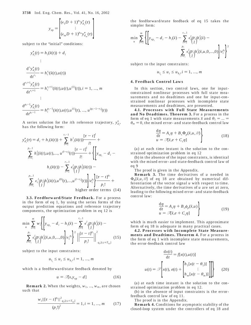
5.1. A Chemical Reactor with Time Delay. Con-sider two constant-volume, isothermal, continuous-stirred-tank reactors in series, as shown in Figure 1, inwhich the following series reactions take place in theliquid phase:
The rates of formation of A and B per unit volume are
Each reactor has a fresh feed stream consisting of pureA.
The reactor dynamics are represented by the followingmodel:
where x(t) ) [CA1(t) CB1(t) CA2(t) CB2(t)]T, u(t) ) [F1(t)F2(t)]T, and y(t) ) [CB1(t - θ1) CB2(t - θ2)]T with θ1 ) θ2) 300/3600. In addition, CAi ) 7 mol/L, V1 ) V2 ) 0.01L, ul1 ) ul2 ) 0 L h-1, uh1 ) uh2 ) 1.5 × 10⁻² L h-1, kA) 6 L mol-1 h-1, and kB ) 1 h-1.
The following two nonlinear controllers are compared:
(1) the error-feedback control law of eq 20 with p1 )p2 ) 2, ε1 ) 1/8, ε2 ) 1/10, and w1 and w2 set accordingto eq 17
(2) the nonlinear model-predictive controller
subject to
Figure 1. Schematic of the isothermal reactors in series.
A f B f C
RA ) -kACA2
RB ) kACA2 - kBCB
f(x,u) ) [-kAx12 + (CAi
- x1)u1
V1
-u1
V1x2 + kAx1
2 - kBx2
-kAx32 +
u2
V2(CAi
- x3) +u1
V2(x1 - x3)
u1
V2(x2 - x4) -
u2
V2x4 - kBx4 + kAx3
2]
h1(x(t - θ1)) ) x2(t - θ1)
h2(x(t - θ2)) ) x4(t - θ2)
dx1
dt) -kAx1
2 + (CAi- x1)
u1
V1x1(0) ) x10
dx2
dt) -
u1
V1x2 + kAx1
2 - kBx2 x2(0) ) x20(21)
dx3
dt) -kAx3
2 +u2
V2(CAi
- x3) +u1
V2(x1 - x3) x3(0) ) x30
dx4
dt)
u1
V2(x2 - x4) -
u2
V2x4 - kBx4 + kAx3
2 x4(0) ) x40
u ) F (x,e + [x2(t - θ1)x4(t - θ2) ])
h1(x) ) x2
hh11(x,u) ) -
u1
V1x2 + kAx1
2 - kBx2
hh12(x,u) ) 2kAx1[-kAx1
2 +(CAi
- x1)
V1u1] -
(kB +u1
V1)[kAx1
2 - kBx2 -u1
V1x2]
h2(x) ) x4
hh12(x,u) )
u1
V2(x2 - x4) -
u2
V2x4 + kAx3
2 - kBx4
hh22(x,u) )
u1
V2(-
u1
V1x2 + kAx1
2 - kBx2) +
2kAx3(u1
V2(x1 -x3) +
u2
V2(CAi
- x3) - kAx32) -
(u1
V2+
u2
V2+ kB)(u1
V2(x2 - x4) -
u2
V2x4 + kAx3
2 - kBx4)
minuj
∑j)1
2
∑i)1
Pj
aji[yspj(k + i) - yjj
/ (k + i)]2 +
∑j)1
2
∑i)0
Mj-1
bji[uj(k + i) - uj(k + i - 1)]2 (22)
yjj/(k + i) ) hi
j(xj(k),u1(k),u2(k),...,u1(k + i - 1),u2(k +i - 1)) + dj(k + i),
i ) 1, ..., Pj, j ) 1, 2
xj(k + 1) ) Φ(xj(k),u(k))
uj(k + i) ) uj(k + i - 1), i ) Mj, Mj + 1, ..., j ) 1, 2
Ind. Eng. Chem. Res., Vol. 41, No. 16, 2002 3739
Here, Φ(xj(k),u(k)) z xj(k) + ∆t / (f(xj(k)) + g1(xj(k)) ×u1(k) + g2(xj(k)) u2(k)) and
where j ) 1, 2 is the output and manipulated variablecounter, k denotes the current sampling instant, anduj ) [u1(k)...u1(k + M1 - 1) u2(k)...u2(k + M2 - 1)]. Thefollowing parameter values are used: prediction hori-zons: P1 ) P2 ) 2; control horizons: M1 ) M2 ) 1;sampling interval: ∆t ) 1/12(v1 ) v2 ) 1); a11 ) 0, a12) 4 × 10⁶, a21 ) 0, a22 ) 2 × 10², b10 ) 1 × 10¹⁰, and b20) 1 × 10⁶.
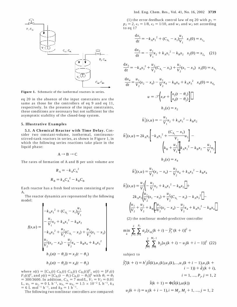
Servo Performance. The process is initially at thesteady state (Ch A1(0) ) 3/4, Ch B1(0) ) 2.1916, Ch A2(0) ) 3/4,Ch B2(0) ) 2.1916). The set points are adjusted to ysp ) [23]T. Figure 2 depicts the closed-loop responses of theprocess outputs and manipulated inputs. The outputresponses under the controller of eq 22 are moreoscillatory and slower. This is because the controller isshortsighted. Even though the prediction horizons ofboth outputs are 2, the sample interval is small andtherefore the time horizon for prediction of 2∆t is small.On the other hand, the controller in eq 21 does not sufferfrom shortsightedness when the same prediction hori-zons are used. A less oscillatory response results. Thecontroller in eq 21 is easier to tune than that in eq 22.It is difficult to select better values for the tuningparameters a11, a12, a21, and a22 in eq 22 since thecontroller is somewhat over-parametrized, and theireffects on speed of the response are not well understoodand monotonic. However, the controller of eq 21 has onlytwo tunable parameters, ε1 and ε2, which are easier totune and whose effects on the response are predictable(the larger their values, the slower the response).
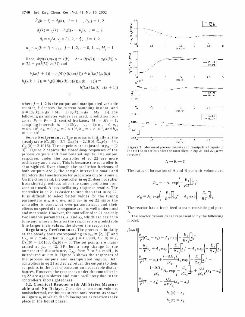
Regulatory Performance. The process is initiallyat the steady state corresponding to ysp ) [2, 3]T andCAip ) 7 mol/L; that is, Ch A1(0) ) 0.6988, Ch B1(0) ) 2,Ch A2(0) ) 1.0133, Ch B2(0) ) 3. The set points are main-tained at ysp ) [2, 3]T, but a step change in theunmeasured disturbance, CAip, from 7 to 8.4 mol/L, isintroduced at t ) 0. Figure 3 shows the responses ofthe process outputs and manipulated inputs. Bothcontrollers in eq 21 and eq 22 return the outputs to theirset points in the face of constant unmeasurable distur-bances. However, the responses under the controller ineq 22 are again slower and more oscillatory due to thecontroller’s shortsightedness.
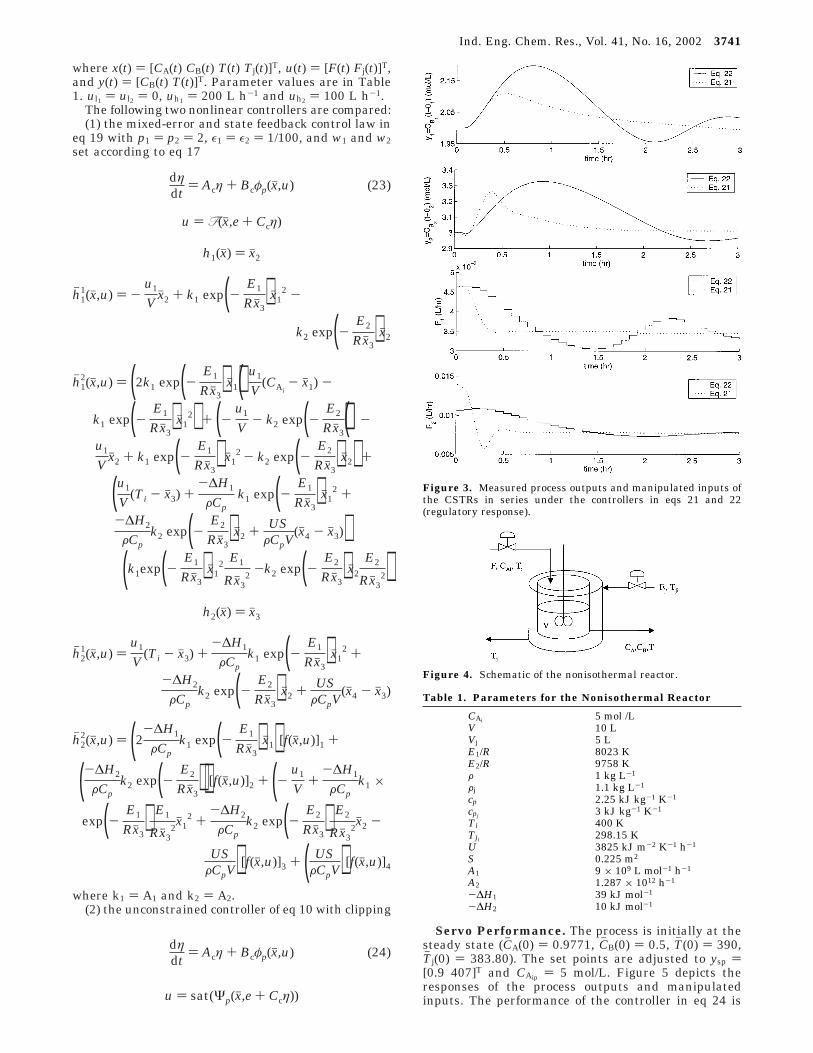
5.2. Chemical Reactor with All States Measur-able and No Delays. Consider a constant-volume,nonisothermal, continuous-stirred-tank reactor, as shownin Figure 4, in which the following series reactions takeplace in the liquid phase:
The rates of formation of A and B per unit volume are
The reactor has a fresh feed stream consisting of pureA.
The reactor dynamics are represented by the followingmodel:
dj(k + i) ) dj(k), i ) 1, ..., Pj, j ) 1, 2
dj(k) ) yjj(k) - hj(xj(k - θj)), j ) 1, 2
θj ) vj∆t, vj ∈ {1, 2, ‚‚‚}, j ) 1, 2
ulje uj(k + i) e uhj
, j ) 1, 2, i ) 0, 1, ..., Mj - 1
hj(x(k + 1)) ) hj(Φ(x(k),u(k))) z hj1(x(k),u(k))
hj(x(k + 2)) ) hj(Φ(Φ(x(k),u(k)),u(k + 1))) z
hj2(x(k),u(k),u(k + 1))
l
Figure 2. Measured process outputs and manipulated inputs ofthe CSTRs in series under the controllers in eqs 21 and 22 (servoresponse).
A f B f C
RA ) -A1 exp(-E1
RT)CA2
RB ) A1 exp(-E1
RT)CA2 - A2 exp(-
E2
RT)CB
f(x,u) )
[u1
V(CAi
- x1) - A1 exp(-E1
Rx3)x1
2
-u1
Vx2 + A1 exp(-
E1
Rx3)x1
2 - A2 exp(-E2
Rx3)x2
u1
V(Ti - x3) +
(-∆H1)Fcp
A1 exp(-E1
Rx3)x1
2 +
(-∆H2)Fcp
A2 exp(-E2
Rx3)x2 + US
FcpV(x4 - x3)
u2
V(Tji
- x4) - USFjVjcpj
(x4 - x3)]
h1(x) ) x2
h2(x) ) x3
3740 Ind. Eng. Chem. Res., Vol. 41, No. 16, 2002
where x(t) ) [CA(t) CB(t) T(t) Tj(t)]T, u(t) ) [F(t) Fj(t)]T,and y(t) ) [CB(t) T(t)]T. Parameter values are in Table1. ul1 ) ul2 ) 0, uh1 ) 200 L h-1 and uh2 ) 100 L h-1.
The following two nonlinear controllers are compared:(1) the mixed-error and state feedback control law in
eq 19 with p1 ) p2 ) 2, ε1 ) ε2 ) 1/100, and w1 and w2set according to eq 17
where k1 ) A1 and k2 ) A2.(2) the unconstrained controller of eq 10 with clipping
Servo Performance. The process is initially at thesteady state (Ch A(0) ) 0.9771, Ch B(0) ) 0.5, Th (0) ) 390,Th j(0) ) 383.80). The set points are adjusted to ysp )[0.9 407]T and CAip ) 5 mol/L. Figure 5 depicts theresponses of the process outputs and manipulatedinputs. The performance of the controller in eq 24 is
dηdt
) Acη + Bcφp(xj,u) (23)
u ) F(xj,e + Ccη)
h1(xj) ) xj2
hh11(xj,u) ) -
u1
Vxj2 + k1 exp(-
E1
Rxj3)xj1
2 -
k2 exp(-E2
Rxj3)xj2
hh12(xj,u) ) (2k1 exp(-
E1
Rxj3)xj1)(u1
V(CAi
- xj1) -
k1 exp(-E1
Rxj3)xj1
2) + (-u1
V- k2 exp(-
E2
Rxj3))(-
u1
Vxj2 + k1 exp(-
E1
Rxj3) xj1
2 - k2 exp(-E2
Rxj3)xj2) +
(u1
V(Ti - xj3) +
-∆H1
FCpk1 exp(-
E1
Rxj3)xj1
2 +
-∆H2
FCpk2 exp(-
E2
Rxj3)xj2 + US
FCpV(xj4 - xj3))
(k1exp(-E1
Rxj3)xj1
2 E1
Rxj32
-k2 exp(-E2
Rxj3)xj2
E2
Rxj32)
h2(xj) ) xj3
hh21(xj,u) )
u1
V(Ti - xj3) +
-∆H1
FCpk1 exp(-
E1
Rxj3)xj1
2 +
-∆H2
FCpk2 exp(-
E2
Rxj3)xj2 + US
FCpV(xj4 - xj3)
hh22(xj,u) ) (2-∆H1
FCpk1 exp(-
E1
Rxj3)xj1)[f(xj,u)]1 +
(-∆H2
FCpk2 exp(-
E2
Rxj3))[f(xj,u)]2 + (-
u1
V+
-∆H1
FCpk1 ×
exp(-E1
Rxj3) E1
Rxj32xj1
2 +-∆H2
FCpk2 exp(-
E2
Rxj3) E2
Rxj32xj2 -
USFCpV)[f(xj,u)]3 + ( US
FCpV)[f(xj,u)]4
dηdt
) Acη + Bcφp(xj,u) (24)
u ) sat(Ψp(xj,e + Ccη))
Figure 3. Measured process outputs and manipulated inputs ofthe CSTRs in series under the controllers in eqs 21 and 22(regulatory response).
Figure 4. Schematic of the nonisothermal reactor.
Table 1. Parameters for the Nonisothermal Reactor
CAi 5 mol /LV 10 LVj 5 LE1/R 8023 KE2/R 9758 KF 1 kg L-1
Fj 1.1 kg L-1
cp 2.25 kJ kg-1 K-1
cpj 3 kJ kg-1 K-1
Ti 400 KTji 298.15 KU 3825 kJ m-2 K-1 h-1
S 0.225 m2
A1 9 × 10⁹ L mol-1 h-1
A2 1.287 × 10¹² h-1
-∆H1 39 kJ mol-1
-∆H2 10 kJ mol-1
Ind. Eng. Chem. Res., Vol. 41, No. 16, 2002 3741
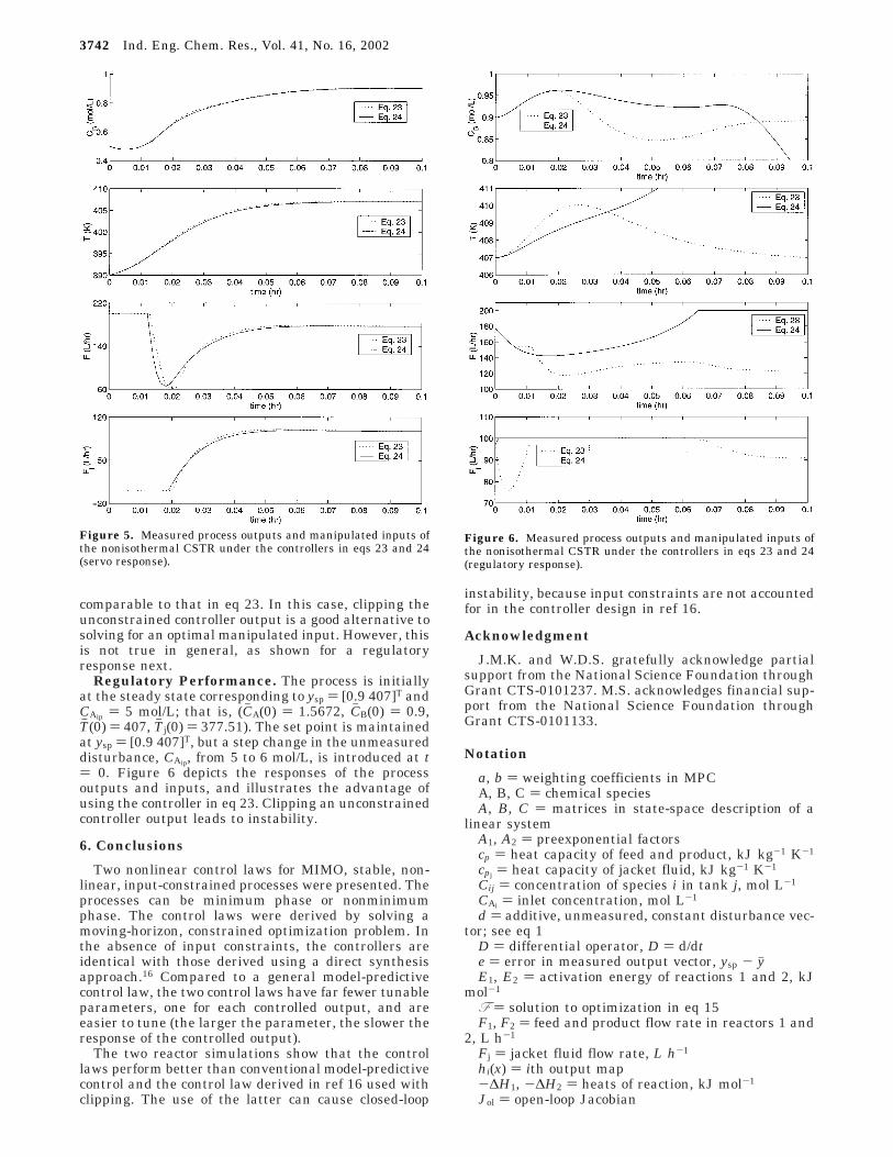
comparable to that in eq 23. In this case, clipping theunconstrained controller output is a good alternative tosolving for an optimal manipulated input. However, thisis not true in general, as shown for a regulatoryresponse next.
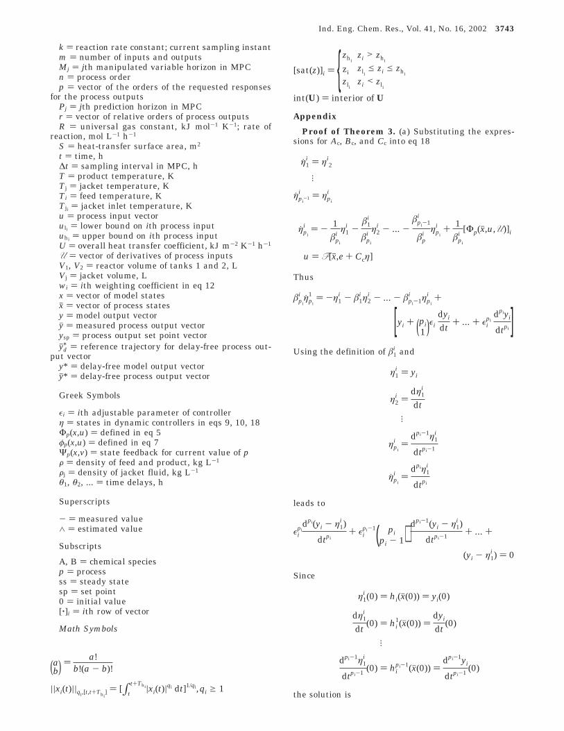
Regulatory Performance. The process is initiallyat the steady state corresponding to ysp ) [0.9 407]T andCAip ) 5 mol/L; that is, (Ch A(0) ) 1.5672, Ch B(0) ) 0.9,Th (0) ) 407, Th j(0) ) 377.51). The set point is maintainedat ysp ) [0.9 407]T, but a step change in the unmeasureddisturbance, CAip, from 5 to 6 mol/L, is introduced at t) 0. Figure 6 depicts the responses of the processoutputs and inputs, and illustrates the advantage ofusing the controller in eq 23. Clipping an unconstrainedcontroller output leads to instability.
6. Conclusions
Two nonlinear control laws for MIMO, stable, non-linear, input-constrained processes were presented. Theprocesses can be minimum phase or nonminimumphase. The control laws were derived by solving amoving-horizon, constrained optimization problem. Inthe absence of input constraints, the controllers areidentical with those derived using a direct synthesisapproach.16 Compared to a general model-predictivecontrol law, the two control laws have far fewer tunableparameters, one for each controlled output, and areeasier to tune (the larger the parameter, the slower theresponse of the controlled output).
The two reactor simulations show that the controllaws perform better than conventional model-predictivecontrol and the control law derived in ref 16 used withclipping. The use of the latter can cause closed-loop
instability, because input constraints are not accountedfor in the controller design in ref 16.
Acknowledgment
J.M.K. and W.D.S. gratefully acknowledge partialsupport from the National Science Foundation throughGrant CTS-0101237. M.S. acknowledges financial sup-port from the National Science Foundation throughGrant CTS-0101133.
Notation
a, b ) weighting coefficients in MPCA, B, C ) chemical speciesA, B, C ) matrices in state-space description of a
linear systemA1, A2 ) preexponential factorscp ) heat capacity of feed and product, kJ kg-1 K-1
cpj ) heat capacity of jacket fluid, kJ kg-1 K-1
Cij ) concentration of species i in tank j, mol L-1
CAi ) inlet concentration, mol L-1
d ) additive, unmeasured, constant disturbance vec-tor; see eq 1
D ) differential operator, D ) d/dte ) error in measured output vector, ysp - yjE1, E2 ) activation energy of reactions 1 and 2, kJ
mol-1
F ) solution to optimization in eq 15F1, F2 ) feed and product flow rate in reactors 1 and
2, L h-1
Fj ) jacket fluid flow rate, L h-1
hi(x) ) ith output map-∆H1, -∆H2 ) heats of reaction, kJ mol-1
Jol ) open-loop Jacobian
Figure 5. Measured process outputs and manipulated inputs ofthe nonisothermal CSTR under the controllers in eqs 23 and 24(servo response).
Figure 6. Measured process outputs and manipulated inputs ofthe nonisothermal CSTR under the controllers in eqs 23 and 24(regulatory response).
3742 Ind. Eng. Chem. Res., Vol. 41, No. 16, 2002
k ) reaction rate constant; current sampling instantm ) number of inputs and outputsMj ) jth manipulated variable horizon in MPCn ) process orderp ) vector of the orders of the requested responses
for the process outputsPj ) jth prediction horizon in MPCr ) vector of relative orders of process outputsR ) universal gas constant, kJ mol-1 K-1; rate of
reaction, mol L-1 h-1
S ) heat-transfer surface area, m2
t ) time, h∆t ) sampling interval in MPC, hT ) product temperature, KTj ) jacket temperature, KTi ) feed temperature, KTji ) jacket inlet temperature, Ku ) process input vectoruli ) lower bound on ith process inputuhi ) upper bound on ith process inputU ) overall heat transfer coefficient, kJ m-2 K-1 h-1
U ) vector of derivatives of process inputsV1, V2 ) reactor volume of tanks 1 and 2, LVj ) jacket volume, Lwi ) ith weighting coefficient in eq 12x ) vector of model statesxj ) vector of process statesy ) model output vectoryj ) measured process output vectorysp ) process output set point vectoryjd/ ) reference trajectory for delay-free process out-
put vectory* ) delay-free model output vectoryj* ) delay-free process output vector
Greek Symbols
εi ) ith adjustable parameter of controllerη ) states in dynamic controllers in eqs 9, 10, 18Φp(x,u) ) defined in eq 5φp(x,u) ) defined in eq 7Ψp(x,v) ) state feedback for current value of pF ) density of feed and product, kg L-1
Fj ) density of jacket fluid, kg L-1
θ1, θ2, ... ) time delays, h
Superscripts
- ) measured value∧ ) estimated value
Subscripts
A, B ) chemical speciesp ) processss ) steady statesp ) set point0 ) initial value[‚]i ) ith row of vector
Math Symbols
Appendix
Proof of Theorem 3. (a) Substituting the expres-sions for Ac, Bc, and Cc into eq 18
Thus
Using the definition of â1i and
leads to
Since
the solution is
(ab) ) a!b!(a - b)!
||xi(t)||qi,[t,t+Thi] ) [∫t
t+Thi|xi(t)|qi dt]1/qi,qi g 1
[sat(z)]i ) {zhizi > zhi
zi zlie zi e zhi
zlizi < zli
int(U) ) interior of U
η1i ) ηi
2
l
ηpi-1
i ) ηpi
i
ηpi
i ) - 1âpi
iη1
i -â1
i
âpi
iη2
i - ... -âpi-1
i
âpi
ηpi
i + 1âpi
i[Φp(xj,u,U)]i
u ) F[xj,e + Ccη]
âpi
i ηpi
1 ) -η1i - â1
i η2i - ... - âpi-1
i ηpi
i +
[yi + (pi1)εi
dyi
dt+ ... + εi
pidpiyi
dtpi ]η1
i ) yi
η2i )
dη1i
dt
l
ηpi
i )dpi-1η1
i
dtpi-1
ηpi
i )dpiη1
i
dtpi
εipidpi(yi - η1
i )
dtpi+ εi
pi-1( pipi - 1) dpi-1(yi - η1
i )
dtpi-1+ ... +
(yi - η1i ) ) 0
η1i (0) ) hi(xj(0)) ) yi(0)
dη1i
dt(0) ) hi
1(xj(0)) )dyi
dt(0)
l
dpi-1η1i
dtpi-1(0) ) hi
pi-1(xj(0)) )dpi-1yi
dtpi-1(0)
Ind. Eng. Chem. Res., Vol. 41, No. 16, 2002 3743
Therefore
which implies
Thus, u is the solution to eq 15, which is equivalent tothe optimization in eq 12.
(b) In the absence of input constraints, under theassumption that the global minimum of the performanceindex is always reached, the control action is thesolution of
Denoting the solution to the m algebraic equations asu ) Ψp(xj,e + Ccη) gives the control law in eq 9.
Proof of Theorem 4. (a) Since x(0) ) xj(0), x(t) ) xj(t)∀ t g 0. Therefore, the controller in eq 20 is
However, e + h(xj(t - θ)) ) ysp - yj + h(xj(t - θ)) ) ysp -h(xj(t - θ)) - d + h(xj(t - θ)) ) ysp - d, implying thecontroller is
which is the solution to the optimization in eq 12.(b) In the absence of input constraints, under the
assumption that the global minimum of the performanceindex is always reached, the control action is thesolution of
Denoting the solution to the m algebraic equations asu ) Ψp(xj,e + h(x(t - θ))) gives the control law ineq 11.
Literature Cited(1) De Nicolao, G.; Magni, L.; Scattolini, R. Stabilizing Reced-
ing-Horizon Control of Nonlinear Time-Varying Systems. IEEETrans. Autom. Control 1998, 43, 1030.
(2) Chen, H.; Allgower, F. A Quasi-infinite Horizon NonlinearModel Predictive Control Scheme with Guaranteed Stability.Automatica 1998, 34, 1205.
(3) Kravaris, C.; Daoutidis, P. Nonlinear State FeedbackControl of Second-Order Nonminimum Phase Nonlinear Systems.Comput. Chem. Eng. 1990, 14, 439.
(4) Doyle, F. J., III; Allgower, F.; Morari, M. A Normal FormApproach to Approximate Input-Output Linearization for Maxi-mum Phase Nonlinear SISO Systems. IEEE Trans. Autom. Control1996, 41, 305.
(5) Wright, R. A.; Kravaris, C. Nonminimum Phase Compensa-tion for Nonlinear Processes. AIChE J. 1992, 38, 26.
(6) Kravaris, C.; Niemiec, M.; Berber, R.; Brosilow, C. B.Nonlinear Model-based Control of Nonminimum-phase Processes.In Nonlinear Model Based Process Control; Berber, R., Kravaris,C., Eds.; Kluwer: Dordrecht, 1998.
(7) Niemiec, M.; Kravaris, C. Controller Synthesis for Multi-variable Nonlinear Nonminimum-phase Processes. Proc. ACC1998, 2076.
(8) Isidori, A.; Byrnes, C. I. Output Regulation of NonlinearSystems. IEEE Trans. Autom. Control 1990, 35, 131.
(9) Isidori, A.; Astolfi, A. Disturbance Attenuation and H∞Control via Measurement Feedback in Nonlinear Systems. IEEETrans. Autom. Control 1992, 37, 1283.
(10) van der Schaft, A. J. L2 Gain Analysis of NonlinearSystems and Nonlinear State Feedback H∞ Control. IEEE Trans.Autom. Control 1992, 37, 770.
(11) Chen, D.; Paden, B. Stable Inversion of Nonlinear Non-minimum-phase Systems. Int. J. Control 1996, 64, 81.
(12) Hunt, L. R.; Meyer, G. Stable Inversion for NonlinearSystems. Automatica 1997, 33, 1549.
(13) Devasia, S.; Chen, D.; Paden, B. Nonlinear Inversion-basedOutput Tracking. IEEE Trans. Autom. Control 1996, 41, 930.
(14) Devasia, S. Approximated Stable Inversion for NonlinearSystems with Nonhyperbolic Internal Dynamics. IEEE Trans.Autom. Control 1999, 44, 1419.
(15) Isidori, A. Nonlinear Control Systems; Springer-Verlag:New York, 1995.
(16) Kanter, J.; Soroush, M.; Seider, W. D. Continuous-time,Nonlinear Feedback Control of Multivariable Stable Processes.Submitted for publication in J. Process Control.
(17) Hirschorn, R. M. Invertibility of Nonlinear Systems. SIAMJ. Control Optim. 1979, 17, 289.
Received for review June 13, 2001Revised manuscript received August 20, 2001
IE0105066
η1i ) yi ) hi(xj), i ) 1, ..., m; t g 0
e + Ccη ) e + h(xj) ) ysp - h(xj) - d + h(xj) ) ysp - d
u ) F[xj,e + Ccη] ) F[xj,ysp - d]
dηdt
) Acη + BcΦp(xj,u,U)
0 ) [[ei + [Cc]iη - hi(xj(t)) -
∑l)1
ri-1
εi
l(pil )hi
l(xj(t)) - ∑l)ri
pi
εi
l(pil )hh i
l(xj(t),u(t))]/εi
pi]i ) 1, ..., m
u(t) ) F[xj(t),e(t) + h(xj(t - θ))]
dxjdt
) f[xj(t),u(t)]
u ) F[xj,ysp - d]
dxjdt
) f(xj,u)
dxdt
) f(x,u)
0 ) [ei + hi(x(t - θi)) - hi(xj(t)) -
∑l)1
ri-1
εi
l(pil )hi
l(xj(t)) - ∑l)ri
pi
εi
l(pil )hh i
l]/εi
pi
i ) 1, ..., m
3744 Ind. Eng. Chem. Res., Vol. 41, No. 16, 2002