Nonlinear Finite Element Analysis and Post-Processing of Reinforced

Concrete Structures under Transient Creep Strain

by

Akira Jodai

A thesis submitted in conformity with the requirements

for the degree of Master of Applied Science Graduate Department of Civil Engineering

University of Toronto

© Copyright Akira Jodai (2013)

i

Nonlinear Finite Element Analysis and Post-Processing of Reinforced Concrete

Structures under Transient Creep Strain

Akira Jodai

Master of Applied Science Graduate Department of Civil Engineering

University of Toronto 2013

Abstract

A suite of NLFEA programs, VecTor, has been developed at the University of Toronto.

However, this software still requires the development of other functions to execute some types

of analyses. One of the required functions is the consideration of transient creep strain in the

heat transfer analysis. Moreover, there is a strong need to develop a general graphics-based post-

processor applicable to VecTor programs.

The first objective of this thesis is to develop a function considering the effect of the transient

creep strain, because it can have significant influence on the behaviour of concrete under

elevated temperatures. The second purpose of this thesis is to construct the new analysis

visualization features compatible with entire suite of VecTor programs. As the result, the

modified post-processor, JANUS, has had its abilities expanded significantly.

ii

Acknowledgements

Firstly, I would like to express my gratitude to Professor Frank J. Vecchio for his support and

guidance. I thank him for motivating me to achieve the good result of the project.

Great appreciation is also given to Professor Shamim A. Sheikh for his suggestion and

knowledge in the review of this thesis.

I would like to thank Fady ElMohandes for his assistance with VecTor3 and Ivan Chak for his

help with JANUS programming.

I gratefully acknowledge the support through the employee scholarship program from Kajima

Corporation.

Finally, I dedicate my thesis to my family, Hitomi, Itsuki and Ren who support and encourage

me every time.

iii

Table of contents

Abstract ................................................................................................................................i

Acknowledgements..............................................................................................................ii

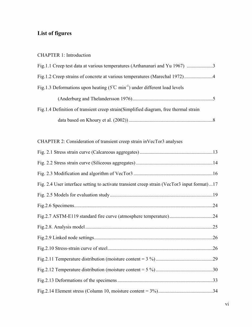
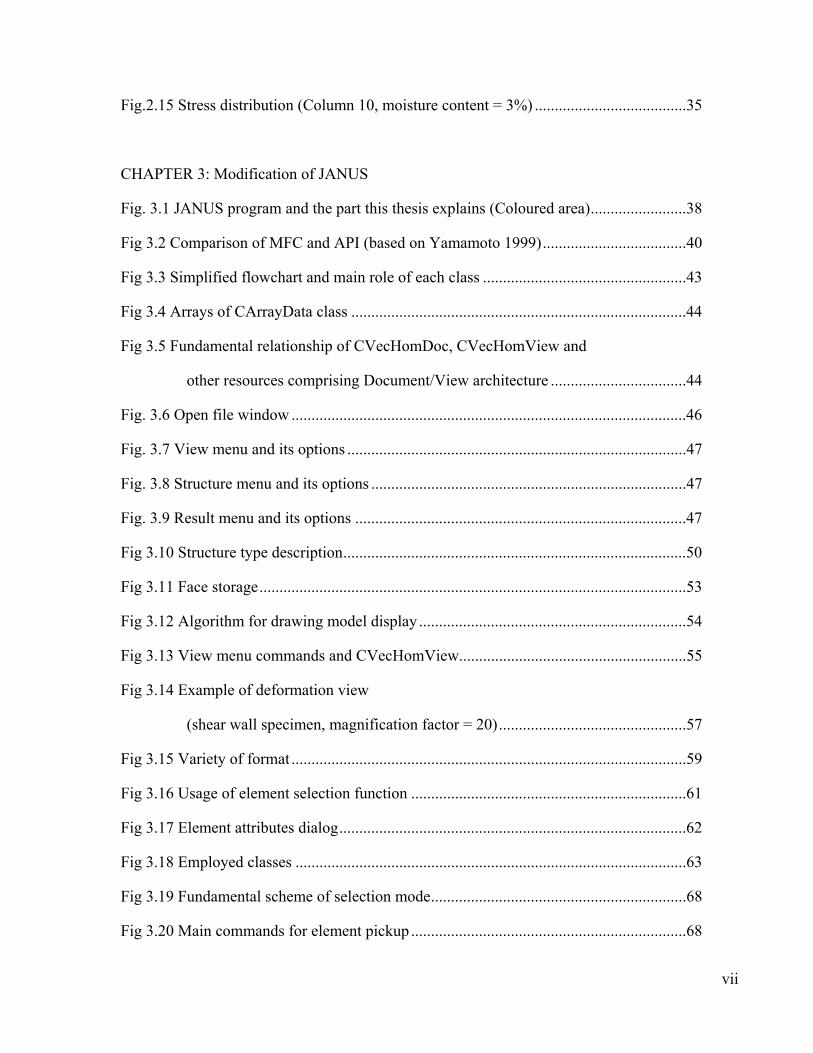
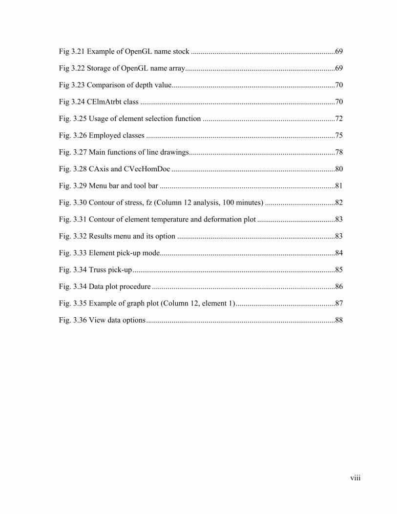
List of figures .......................................................................................................................vi

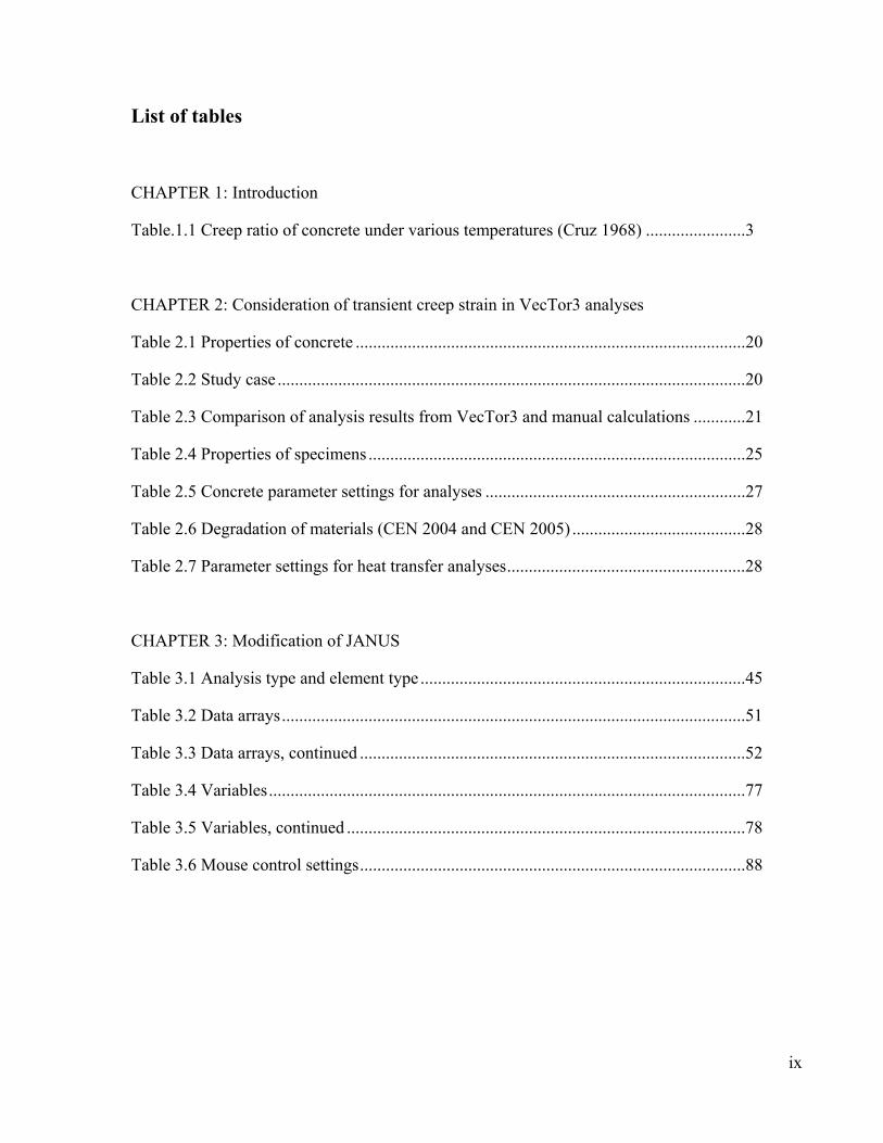
List of tables ........................................................................................................................ix

CHAPTER 1: Introduction ..................................................................................................1

1.1 Creep of concrete under room temperature ...................................................................1

1.2 Experimental data of creep under high temperatures ....................................................2

1.3 Transient strain of concrete ...........................................................................................5

1.4 Modeling creep stain and transient strain under high temperatures ..............................6

1.5 Coupling effects of creep strain and transient strain .....................................................7

1.6 Modeling the coupling effects .......................................................................................9

1.7 Modification of VecTor and JANUS .............................................................................10

CHAPTER 2: Consideration of transient creep strain in VecTor3 analyses .......................11

2.1 Formulation of transient creep strain .............................................................................11

2.1.1 Modeling transient creep strain ..................................................................11

2.1.2 Algorithm ...................................................................................................15

2.3 Evaluation study ............................................................................................................18

2.3.1 Evaluation study with simple model ..........................................................18

2.3.2 Evaluation study with complex model .......................................................22

2.4 Summary ........................................................................................................................36

iv

CHAPTER 3: Modification of JANUS ...............................................................................37

3.1 Introduction ...................................................................................................................37

3.1.1 Background ................................................................................................37

3.1.2 Objectives of the study ...............................................................................38

3.2 Development environment and architecture ..................................................................40

3.2.1 Development environment .........................................................................40

3.2.2 Open GL .....................................................................................................41

3.2.3 Structure and architecture of JANUS .........................................................41

3.3 Accommodations for VecTor series ..............................................................................45

3.3.1 Usage ..........................................................................................................45

3.3.2 Classes, functions and arrays .....................................................................48

3.3.3 Reading process .........................................................................................48

3.3.4 Model display .............................................................................................53

3.3.5 View menu .................................................................................................54

3.3.6 Structure menu ...........................................................................................55

3.3.7 Results menu ..............................................................................................56

3.3.8 Accommodation of old format output ........................................................57

3.4 Element attributes indication .........................................................................................60

3.4.1 Usage ..........................................................................................................60

3.4.2 Modification and classes ............................................................................60

3.4.3 Element pick-up .........................................................................................64

3.4.4 Extraction of element attributes .................................................................66

3.4.5 Indication of element attributes ..................................................................67

3.4.6 Indication of previous display ....................................................................67

3.5 Graph and data generating functions .............................................................................71

v

3.5.1 Usage ..........................................................................................................71

3.5.2 Classes ........................................................................................................74

3.5.3 Data generation and graph plot ..................................................................76

3.5.4 Axis change ................................................................................................79

3.5.5 File output ..................................................................................................79

3.6 Example application ......................................................................................................81

3.6.1 Opening file ................................................................................................81

3.6.2 Results menu and its options ......................................................................82

3.6.3 Element pick-up .........................................................................................84

3.6.4 Graph tool...................................................................................................86

3.6.5 View control ...............................................................................................87

CHAPTER 4: Conclusions ..................................................................................................89

References............................................................................................................................91

vi

List of figures

CHAPTER 1: Introduction

Fig.1.1 Creep test data at various temperatures (Arthananari and Yu 1967) .....................3

Fig.1.2 Creep strains of concrete at various temperatures (Marechal 1972) .......................4

Fig.1.3 Deformations upon heating (5℃ min-1) under different load levels

(Anderburg and Thelandersson 1976) .................................................................5

Fig.1.4 Definition of transient creep strain(Simplified diagram, free thermal strain

data based on Khoury et al. (2002)) ....................................................................8

CHAPTER 2: Consideration of transient creep strain inVecTor3 analyses

Fig. 2.1 Stress strain curve (Calcareous aggregates) ...........................................................13

Fig. 2.2 Stress strain curve (Siliceous aggregates) ..............................................................14

Fig. 2.3 Modification and algorithm of VecTor3 ................................................................16

Fig. 2.4 User interface setting to activate transient creep strain (VecTor3 input format) ...17

Fig. 2.5 Models for evaluation study ...................................................................................19

Fig.2.6 Specimens ................................................................................................................24

Fig.2.7 ASTM-E119 standard fire curve (atmosphere temperature) ...................................24

Fig.2.8. Analysis model .......................................................................................................25

Fig.2.9 Linked node settings ................................................................................................26

Fig.2.10 Stress-strain curve of steel .....................................................................................26

Fig.2.11 Temperature distribution (moisture content = 3 %) ..............................................29

Fig.2.12 Temperature distribution (moisture content = 5 %) ..............................................30

Fig.2.13 Deformations of the specimens .............................................................................33

Fig.2.14 Element stress (Column 10, moisture content = 3%) ............................................34

vii

Fig.2.15 Stress distribution (Column 10, moisture content = 3%) ......................................35

CHAPTER 3: Modification of JANUS

Fig. 3.1 JANUS program and the part this thesis explains (Coloured area) ........................38

Fig 3.2 Comparison of MFC and API (based on Yamamoto 1999) ....................................40

Fig 3.3 Simplified flowchart and main role of each class ...................................................43

Fig 3.4 Arrays of CArrayData class ....................................................................................44

Fig 3.5 Fundamental relationship of CVecHomDoc, CVecHomView and

other resources comprising Document/View architecture ..................................44

Fig. 3.6 Open file window ...................................................................................................46

Fig. 3.7 View menu and its options .....................................................................................47

Fig. 3.8 Structure menu and its options ...............................................................................47

Fig. 3.9 Result menu and its options ...................................................................................47

Fig 3.10 Structure type description ......................................................................................50

Fig 3.11 Face storage ...........................................................................................................53

Fig 3.12 Algorithm for drawing model display ...................................................................54

Fig 3.13 View menu commands and CVecHomView.........................................................55

Fig 3.14 Example of deformation view

(shear wall specimen, magnification factor = 20) ...............................................57

Fig 3.15 Variety of format ...................................................................................................59

Fig 3.16 Usage of element selection function .....................................................................61

Fig 3.17 Element attributes dialog .......................................................................................62

Fig 3.18 Employed classes ..................................................................................................63

Fig 3.19 Fundamental scheme of selection mode ................................................................68

Fig 3.20 Main commands for element pickup .....................................................................68

viii

Fig 3.21 Example of OpenGL name stock ..........................................................................69

Fig 3.22 Storage of OpenGL name array.............................................................................69

Fig 3.23 Comparison of depth value....................................................................................70

Fig 3.24 CElmAtrbt class ....................................................................................................70

Fig. 3.25 Usage of element selection function ....................................................................72

Fig. 3.26 Employed classes .................................................................................................75

Fig. 3.27 Main functions of line drawings ...........................................................................78

Fig. 3.28 CAxis and CVecHomDoc ....................................................................................80

Fig. 3.29 Menu bar and tool bar ..........................................................................................81

Fig. 3.30 Contour of stress, fz (Column 12 analysis, 100 minutes) ....................................82

Fig. 3.31 Contour of element temperature and deformation plot ........................................83

Fig. 3.32 Results menu and its option .................................................................................83

Fig. 3.33 Element pick-up mode..........................................................................................84

Fig. 3.34 Truss pick-up ........................................................................................................85

Fig. 3.34 Data plot procedure ..............................................................................................86

Fig. 3.35 Example of graph plot (Column 12, element 1) ...................................................87

Fig. 3.36 View data options .................................................................................................88

ix

List of tables

CHAPTER 1: Introduction

Table.1.1 Creep ratio of concrete under various temperatures (Cruz 1968) .......................3

CHAPTER 2: Consideration of transient creep strain in VecTor3 analyses

Table 2.1 Properties of concrete ..........................................................................................20

Table 2.2 Study case ............................................................................................................20

Table 2.3 Comparison of analysis results from VecTor3 and manual calculations ............21

Table 2.4 Properties of specimens .......................................................................................25

Table 2.5 Concrete parameter settings for analyses ............................................................27

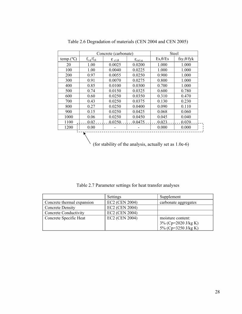
Table 2.6 Degradation of materials (CEN 2004 and CEN 2005) ........................................28

Table 2.7 Parameter settings for heat transfer analyses .......................................................28

CHAPTER 3: Modification of JANUS

Table 3.1 Analysis type and element type ...........................................................................45

Table 3.2 Data arrays ...........................................................................................................51

Table 3.3 Data arrays, continued .........................................................................................52

Table 3.4 Variables ..............................................................................................................77

Table 3.5 Variables, continued ............................................................................................78

Table 3.6 Mouse control settings .........................................................................................88

1

CHAPTER 1: Introduction

Some structures, such as fuel containers and highway bridges, must be designed for conditions

of high temperatures or fire. For these designs, temperature effects on the concrete materials

used for the structures under elevated temperatures are very important. If an analysis including

high temperatures is carried out, the designers may have to consider creep strain and transient

strain, which are quite complex phenomena. This chapter will discuss the creep and transient

response of concrete, and then will consider the coupling effect of creep strain and transient

strain.

1.1 Creep of concrete under room temperature

Creep or relaxation is defined as the long-term deformation of concrete under loading without

drying and temperature effects. Long-term stress under a constant strain without the temperature

effect is called relaxation; in contrast, long-term strain of concrete under a constant stress is

defined as creep (Bazant and Kaplan 1996). According to the authors, these phenomena are

caused by the same mechanisms in concrete materials: long-term applied stress surpasses the

activation energy limit of the material, followed by breaking of the bond in the cement paste.

The creep strain in concrete materials can be described by

( , ) = ( , ) ( ) = ( , ) ( ) (1.1)

where ε (t ',t ): the total strain at time t due to a constant stress

σ(t’): applied stress at time t’,

J(t’, t): creep compliance at time t,

t’: age of the concrete at loading,

2

E0: Yong’s modulus, and

φ (t ',t ): ratio of creep deformation to the initial elastic deformation.

This equation illustrates that the creep of concrete is proportional to the applied stress as well as

time. However, this characteristic is limited only if the stress/strength ratio is below 0.5

(Gvozdev 1966). This figure means that, at high stress levels, the compliance function and the

specific creep become stress dependent.

1.2 Experimental data of creep under high temperatures

When considering deformation under elevated temperatures, there may be two components of

the behaviour. One component is the temperature dependency of the function J(t’, T) in Eq.

(1.1). This dependency means that the creep mechanism is fundamentally same as exhibited at

room temperatures, and this mechanism is accelerated by high temperatures. This model was

proposed by Bazant and Kaplan (1996), and is applicable only when the elevated temperature is

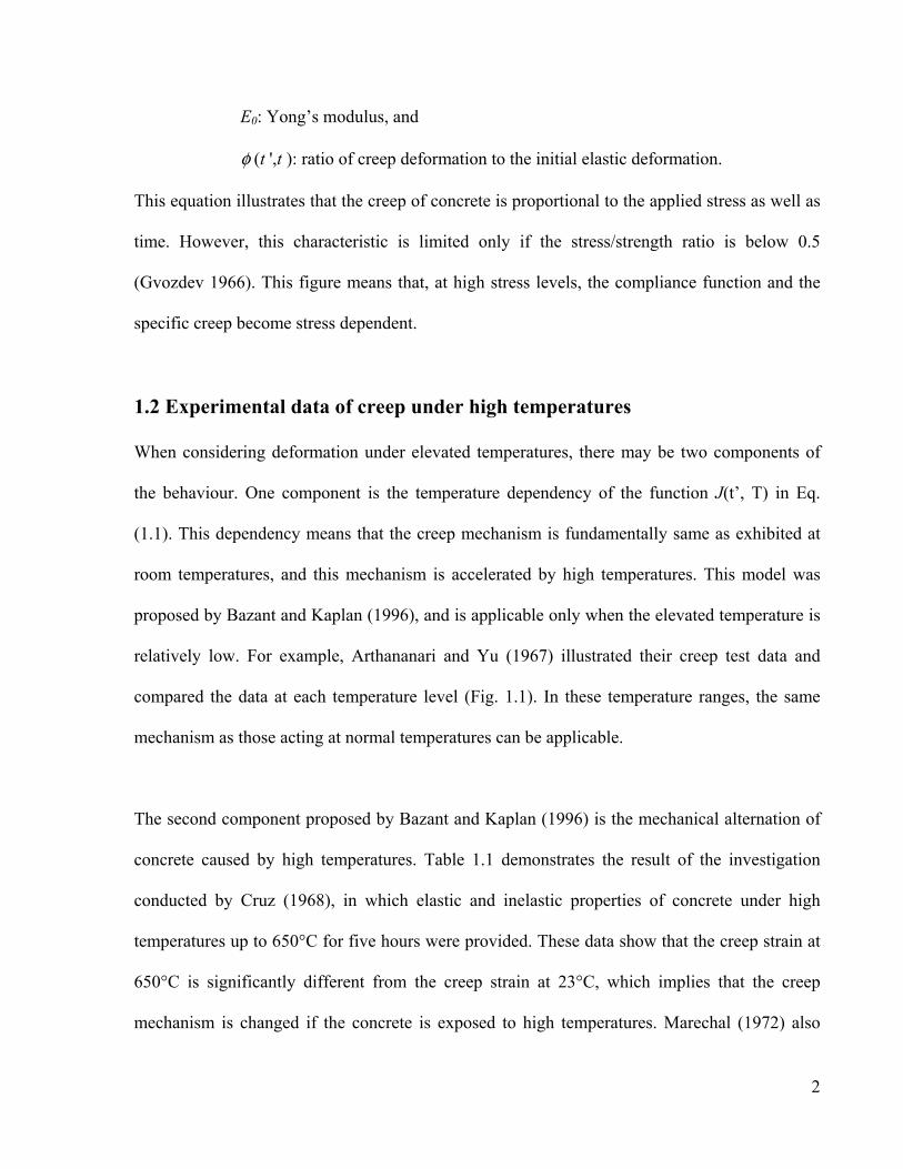
relatively low. For example, Arthananari and Yu (1967) illustrated their creep test data and

compared the data at each temperature level (Fig. 1.1). In these temperature ranges, the same

mechanism as those acting at normal temperatures can be applicable.

The second component proposed by Bazant and Kaplan (1996) is the mechanical alternation of

concrete caused by high temperatures. Table 1.1 demonstrates the result of the investigation

conducted by Cruz (1968), in which elastic and inelastic properties of concrete under high

temperatures up to 650°C for five hours were provided. These data show that the creep strain at

650°C is significantly different from the creep strain at 23°C, which implies that the creep

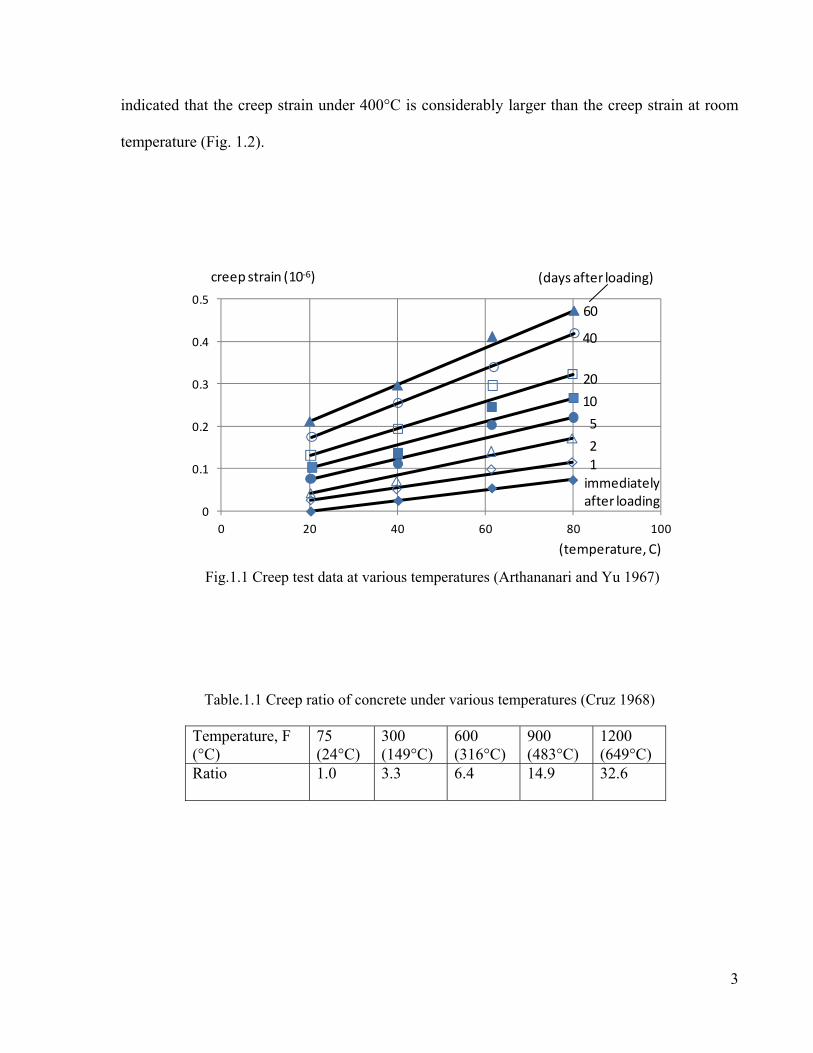
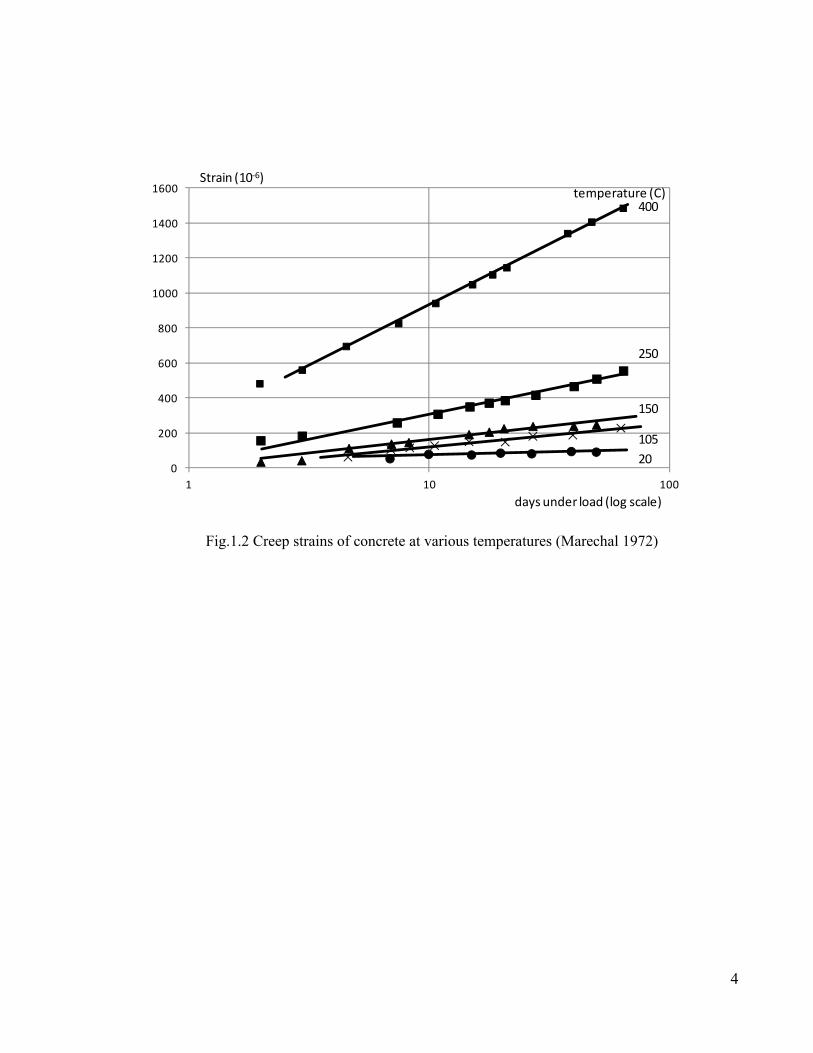
mechanism is changed if the concrete is exposed to high temperatures. Marechal (1972) also

3

indicated that the creep strain under 400°C is considerably larger than the creep strain at room

temperature (Fig. 1.2).

Table.1.1 Creep ratio of concrete under various temperatures (Cruz 1968)

Temperature, F (°C)

75 (24°C)

300 (149°C)

600 (316°C)

900 (483°C)

1200 (649°C)

Ratio 1.0 3.3 6.4 14.9 32.6

Fig.1.1 Creep test data at various temperatures (Arthananari and Yu 1967)

0

0.1

0.2

0.3

0.4

0.5

0 20 40 60 80 100

creep strain (10-6) (days after loading)

125

1020

40

60

immediatelyafter loading

(temperature, C)

4

Fig.1.2 Creep strains of concrete at various temperatures (Marechal 1972)

0

200

400

600

800

1000

1200

1400

1600

1 10 100

Strain (10-6)

days under load (log scale)

temperature (C)400

250

150

10520

5

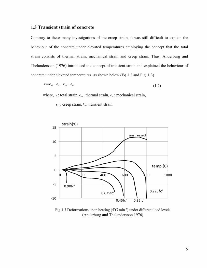
1.3 Transient strain of concrete

Contrary to these many investigations of the creep strain, it was still difficult to explain the

behaviour of the concrete under elevated temperatures employing the concept that the total

strain consists of thermal strain, mechanical strain and creep strain. Thus, Anderburg and

Thelandersson (1976) introduced the concept of transient strain and explained the behaviour of

concrete under elevated temperatures, as shown below (Eq.1.2 and Fig. 1.3).

(1.2)

where, : total strain, : thermal strain, : mechanical strain,

: creep strain, : transient strain

ϵ=ϵth−ϵσ−ϵcr−ϵtr

Fig.1.3 Deformations upon heating (5℃ min-1) under different load levels (Anderburg and Thelandersson 1976)

-10

-5

0

5

10

15

0 200 400 600 800 1000

strain(%)

temp.(C)

unstressed

0.225fc'

0.45fc'

0.675fc'

0.35fc'

0.90fc'

ϵ ϵth ϵσ

ϵcrϵtr

6

1.4 Modeling creep stain and transient strain under high temperatures

Several investigations have produced empirical equations for creep strain and the transient

strain. Schneider (1979) developed models for creep of concrete under high temperatures as

shown below.

(1.3)

where,

E: modulus of elasticity, (1.4)

(1.5)

(1.6)

(1.7)

(1.8)

ω: the moisture content in the concrete in % by weight

Anderberg and Thelandersson (1976) carried out several experiments and developed equations

for creep strain under high temperatures, which are also empirical. As evident in these

equations, the creep strain is expressed as a function of the loading time.

= ( ( )⁄ ) ∙ ∙ ( ) ∙ ( / ) (1.9)

where,

: creep strain

: stress

( ): compression strength of concrete at temperature, T

J (T ,σ )= 1E(1+κ)+Φ

E

g=1.0+σ(T )

fc(20C)(T−20)/100

Φ=g ϕ+σ(T )(T−20)fc(20C)100

ϕ=C1 tanh γω(T−20)+C 2 tanhγ0(T−Tg)+C 3

γω=(0.3ω+2.2)10−3

E=Eo・ F (T )・ g (σ ,T )

7

, 1, : constants

t: time

tr: reference time

Anderberg and Thelandersson (1976) also illustrated that the equation for transient strain is

proportional to stress and thermal strain. According to this model, the transient strain is not a

function of time. Therefore, this equation implies that one may need to consider the effect of

transient strain even if the loading time or the heating time is short.

= − 2 ∙ ∙ ⁄ (1.10)

where,

: transient strain

: thermal strain

: stress

: compressive strength of concrete at room temperature

k2: constant

1.5 Coupling effects of creep strain and transient strain

As illustrated above, many researchers have tried to explain thermal effects on concrete

materials using the concepts of creep strain and transient strain. However, these strains were still

insufficient to explain the concrete behaviour at high temperatures. That means that there might

be an additional important mechanism. Khoury et al (2002) examined the strain-temperature

curve under several load conditions. According to this research, a significant amount of

contraction will occur as the temperature and stress level increase. The difference between the

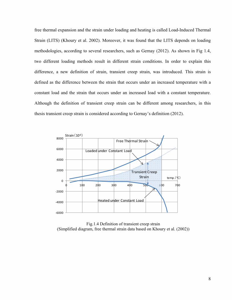
8

free thermal expansion and the strain under loading and heating is called Load-Induced Thermal

Strain (LITS) (Khoury et al. 2002). Moreover, it was found that the LITS depends on loading

methodologies, according to several researchers, such as Gernay (2012). As shown in Fig 1.4,

two different loading methods result in different strain conditions. In order to explain this

difference, a new definition of strain, transient creep strain, was introduced. This strain is

defined as the difference between the strain that occurs under an increased temperature with a

constant load and the strain that occurs under an increased load with a constant temperature.

Although the definition of transient creep strain can be different among researchers, in this

thesis transient creep strain is considered according to Gernay’s definition (2012).

Fig.1.4 Definition of transient creep strain (Simplified diagram, free thermal strain data based on Khoury et al. (2002))

-6000

-4000

-2000

0

2000

4000

6000

8000

0 100 200 300 400 500 600 700

temp.（℃）

Strain（10-6）

Transient Creep Strain

Heated under Constant Load

Free Thermal Strain

Loaded under Constant Load

9

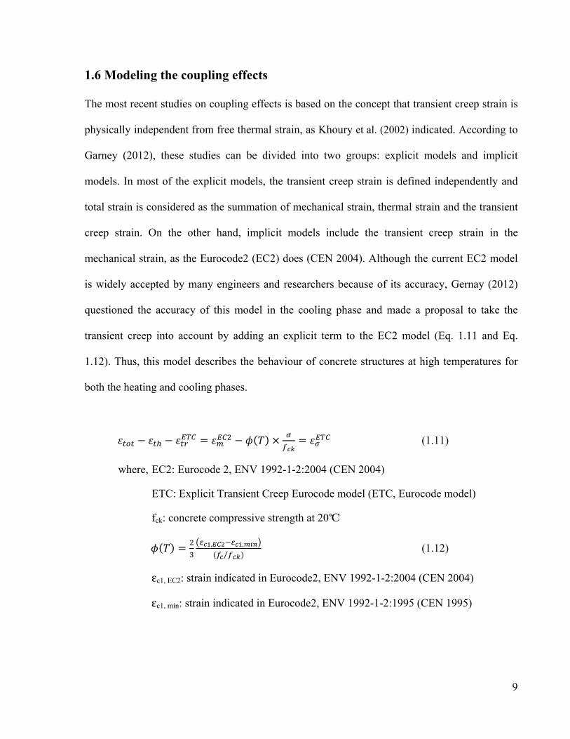
1.6 Modeling the coupling effects

The most recent studies on coupling effects is based on the concept that transient creep strain is

physically independent from free thermal strain, as Khoury et al. (2002) indicated. According to

Garney (2012), these studies can be divided into two groups: explicit models and implicit

models. In most of the explicit models, the transient creep strain is defined independently and

total strain is considered as the summation of mechanical strain, thermal strain and the transient

creep strain. On the other hand, implicit models include the transient creep strain in the

mechanical strain, as the Eurocode2 (EC2) does (CEN 2004). Although the current EC2 model

is widely accepted by many engineers and researchers because of its accuracy, Gernay (2012)

questioned the accuracy of this model in the cooling phase and made a proposal to take the

transient creep into account by adding an explicit term to the EC2 model (Eq. 1.11 and Eq.

1.12). Thus, this model describes the behaviour of concrete structures at high temperatures for

both the heating and cooling phases.

− − = − ( ) × = (1.11)

where, EC2: Eurocode 2, ENV 1992-1-2:2004 (CEN 2004)

ETC: Explicit Transient Creep Eurocode model (ETC, Eurocode model)

fck: concrete compressive strength at 20℃

( ) = , ,( ⁄ ) (1.12)

εc1, EC2: strain indicated in Eurocode2, ENV 1992-1-2:2004 (CEN 2004)

εc1, min: strain indicated in Eurocode2, ENV 1992-1-2:1995 (CEN 1995)

10

1.7 Modification of VecTor and JANUS

VecTor is a suite of nonlinear finite element analysis (NLFEA) programs that is widely used by

researcher and engineers. These programs can execute FE analyses for concrete structures using

the Modified Compression Field Theory (MCFT) (Vecchio and Collins 1986). Moreover, the

VecTor programs have several useful functions to carry out many types of analysis, one of

which is heat transfer analyses. However, the programs still require the development of other

functions to execute some types of analyses. One of the required functions is consideration of

transient creep strain in the heat transfer analysis. As indicated above, when concrete structures

are exposed to higher temperatures, it is necessary to include the transient creep strain in the

analysis, which may have considerable effect on the behaviour of concrete under elevated

temperatures. The other necessity is a proper post-processor to display these outputs: contours of

heat distribution, plots of stress and strain in an element, and graphs of variables. Therefore, in

order to produce a numerical program tool suitable for engineers trying to execute structural fire

calculations, these objectives are addressed in this thesis: analysis with VecTor3 including the

consideration of transient creep strain, and modification of the post-processor JANUS so that the

results of such analyses can be observed.

11

CHAPTER 2: Consideration of transient creep strain in VecTor3 analyses

2.1 Formulation of transient creep strain

2.1.1 Modeling transient creep strain

Gernay (2012) made a proposal to take transient creep into account by adding an explicit term to

the EC2 model (Eq. 2.1 and Eq. 2.2). The transient creep strain is proportional to the applied

stress, and it is considered a part of the total strain. The creep strain in Eq 2.1 is the base creep

strain as a long-term effect. Thus, this creep strain can be neglected under ordinary fire

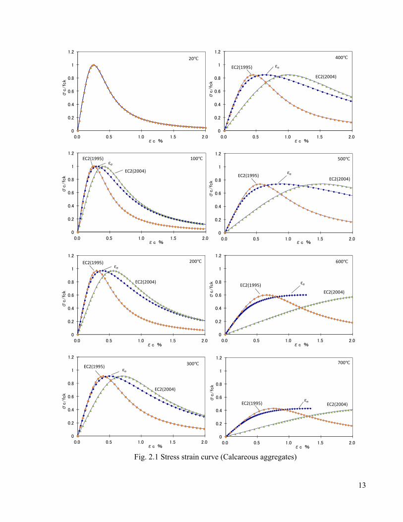
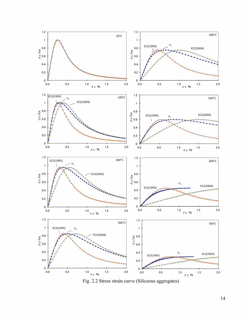
conditions, which usually terminate within 10 hours. Fig. 2.1 and Fig. 2.2 illustrate the old and

new definitions of the stress-strain relationship of EC2, compared to the stress-strain curve

defined in Eq.2.2.

= + + (2.1)

− − = − ( ) × = (2.2)

where,

EC2: Eurocode2, ENV 1992-1-2:2004 (CEN 2004)

ETC: Explicit Transient Creep Eurocode model (ETC, Eurocode model)

fc: concrete compressive strength

fck: concrete compressive strength at 20℃

( ) = , ,( ⁄ ) (2.3)

εtot: total strain

εtr: transient creep strain

12

εcr: basic creep strain, as long term-strain

εth: thermal strain

εσ: stress related strain

εc1, EC2: strain indicated in Eurocode2, ENV 1992-1-2:2004 (CEN 2004)

εc1, min: strain indicated in Eurocode2, ENV 1992-1-2:1995 (CEN 1995)

13

Fig. 2.1 Stress strain curve (Calcareous aggregates)

0

0.2

0.4

0.6

0.8

1

1.2

0.0 0.5 1.0 1.5 2.0

σc/fc

k

εc ％

20℃

0

0.2

0.4

0.6

0.8

1

1.2

0.0 0.5 1.0 1.5 2.0

σc/fc

k

εc ％

100℃EC2(2004)

εσ

EC2(1995)

0

0.2

0.4

0.6

0.8

1

1.2

0.0 0.5 1.0 1.5 2.0

σc/fc

k

εc ％

200℃EC2(2004)

εσEC2(1995)

0

0.2

0.4

0.6

0.8

1

1.2

0.0 0.5 1.0 1.5 2.0

σc/fc

k

εc ％

300℃EC2(2004)

εσEC2(1995)

0

0.2

0.4

0.6

0.8

1

1.2

0.0 0.5 1.0 1.5 2.0

σc/fc

k

εc ％

400℃EC2(2004)

εσEC2(1995)

0

0.2

0.4

0.6

0.8

1

1.2

0.0 0.5 1.0 1.5 2.0

σc/fc

k

εc ％

500℃EC2(2004)

EC2(1995) εσ

0

0.2

0.4

0.6

0.8

1

1.2

0.0 0.5 1.0 1.5 2.0

σc/fc

k

εc ％

600℃EC2(2004)

EC2(1995) εσ

0

0.2

0.4

0.6

0.8

1

1.2

0.0 0.5 1.0 1.5 2.0

σc/fc

k

εc ％

700℃

EC2(2004)EC2(1995)εσ

14

Fig. 2.2 Stress strain curve (Siliceous aggregates)

0

0.2

0.4

0.6

0.8

1

1.2

0.0 0.5 1.0 1.5 2.0

σc/fc

k

εc ％

20℃

0

0.2

0.4

0.6

0.8

1

1.2

0.0 0.5 1.0 1.5 2.0

σc/fc

k

εc ％

EC2(2004)εσ

EC2(1995) 100℃

0

0.2

0.4

0.6

0.8

1

1.2

0.0 0.5 1.0 1.5 2.0

σc/fc

k

εc ％

EC2(2004)

εσ

EC2(1995) 200℃

0

0.2

0.4

0.6

0.8

1

1.2

0.0 0.5 1.0 1.5 2.0

σc/fc

k

εc ％

EC2(2004)

εσEC2(1995)

300℃

0

0.2

0.4

0.6

0.8

1

1.2

0.0 0.5 1.0 1.5 2.0

σc/fc

k

εc ％

EC2(2004)εσEC2(1995)

400℃

0

0.2

0.4

0.6

0.8

1

1.2

0.0 0.5 1.0 1.5 2.0

σc/fc

k

εc ％

EC2(2004)εσEC2(1995)

500℃

0

0.2

0.4

0.6

0.8

1

1.2

0.0 0.5 1.0 1.5 2.0

σc/fc

k

εc ％

EC2(2004)εσ

EC2(1995)

600℃

0

0.2

0.4

0.6

0.8

1

1.2

0.0 0.5 1.0 1.5 2.0

σc/fc

k

εc ％

EC2(2004)εσEC2(1995)

700℃

15

2.1.2 Algorithm

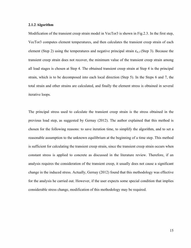
Modification of the transient creep strain model in VecTor3 is shown in Fig.2.3. In the first step,

VecTor3 computes element temperatures, and then calculates the transient creep strain of each

element (Step 2) using the temperatures and negative principal strain εtr,3 (Step 3). Because the

transient creep strain does not recover, the minimum value of the transient creep strain among

all load stages is chosen at Step 4. The obtained transient creep strain at Step 4 is the principal

strain, which is to be decomposed into each local direction (Step 5). In the Steps 6 and 7, the

total strain and other strains are calculated, and finally the element stress is obtained in several

iterative loops.

The principal stress used to calculate the transient creep strain is the stress obtained in the

previous load step, as suggested by Gernay (2012). The author explained that this method is

chosen for the following reasons: to save iteration time, to simplify the algorithm, and to set a

reasonable assumption to the unknown equilibrium at the beginning of a time step. This method

is sufficient for calculating the transient creep strain, since the transient creep strain occurs when

constant stress is applied to concrete as discussed in the literature review. Therefore, if an

analysis requires the consideration of the transient creep, it usually does not cause a significant

change in the induced stress. Actually, Gernay (2012) found that this methodology was effective

for the analysis he carried out. However, if the user expects some special condition that implies

considerable stress change, modification of this methodology may be required.

16

T(STEP)=Tdata :reading temperatures (step 1)

εtr(STEP)=f(T(STEP),σ( STEP -1)) :transient creep strain (step 2)

εtr,3(STEP) =f(εtr

(STEP) ) :calculating principal negative strain (step 3)

εtr,3(STEP)=min(εtr,3

(STEP), εtr,3 (STEP -1)) :choosing minimum principal strain (step 4)

εtr(STEP) =f(εtr,3

(STEP) ) :calculating local strain, εtr,x, εtr,y ….εtr,xz (step 5)

εσ=εm (iter) - ε tr

(STEP ) :calculating stress related strain (step 6)

εσ(iter)=f(T(STEP),σ( iter)) :constitutive law (step 7)

→ σ( iter)

(step 8)

Fig. 2.3 Modification and algorithm of VecTor3

STEP=STEP+1

iter=iter+1

Convergence?

Yes

σ(STEP)= σ(iter)

No

17

Users of VecTor3 are required to input “3” for the “concrete creep and relaxation” input field in

order to activate the algorithm for considering transient creep strain (Fig. 2.4). In addition, it is

strongly recommended that one uses the Eurocode2 (EC2) settings (CEN 2004) for stress-strain

relationships of concrete, because this algorithm is formulated to fit the latest experimental data

by considering the explicit term according to the EC2 definition (Gernay 2012). This means that

the stress-strain relationship of concrete under high temperature can be greatly different from

the experimental data if another definition is selected.

Fig. 2.4 User interface setting to activate transient creep strain (VecTor3 input format)

18

2.3 Evaluation study

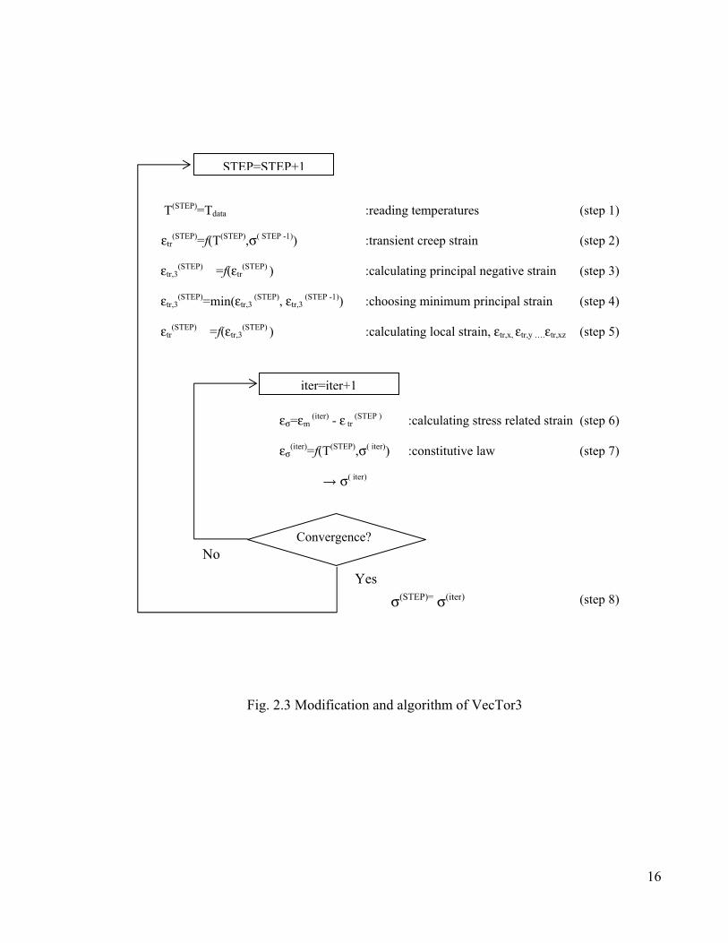
2.3.1 Evaluation study with simple model

In order to confirm that VecTor3 can carry out an analysis correctly with the modifications

made, evaluation studies using simple models and load settings are examined and compared to

manual calculations. In this study, a one-element model under a uniaxial load or a pure shear is

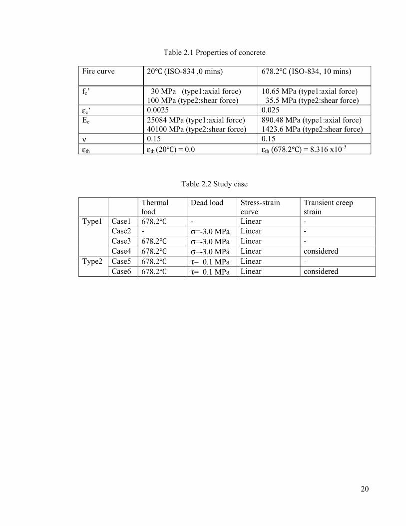
generated (Fig. 2.5). Table 2.1 and Table 2.2 indicate the parameter settings for the evaluation

study. Heat transfer is calculated under the ISO-834 heat curve, and stress and strain are

obtained when the element temperature is 678℃ (10 minutes heating). Degradation of the

concrete material is defined according to Eurocode2 (CEN 2004). The stress-strain relationship

is set as linear because of the need to calculate the results manually.

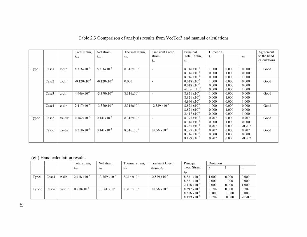
Table 2.3 shows the results of the analysis. Each result agrees with the manual calculation,

indicating that VecTor3 provides precise answers.

19

-Type 1: Axial Force

-Type 2: Pure Shear

Fig. 2.5 Models for evaluation study

x

z

τ=0.1MPa

1000m

1000mm

1000mm

x

z

σ=3.0MPa

1000mm

1000mm

1000mm

20

Table 2.1 Properties of concrete

Fire curve 20℃ (ISO-834 ,0 mins) 678.2℃ (ISO-834, 10 mins)

fc’ 30 MPa (type1:axial force) 100 MPa (type2:shear force)

10.65 MPa (type1:axial force) 35.5 MPa (type2:shear force)

εc’ 0.0025 0.025 Ec 25084 MPa (type1:axial force)

40100 MPa (type2:shear force) 890.48 MPa (type1:axial force) 1423.6 MPa (type2:shear force)

ν 0.15 0.15 εth εth (20℃) = 0.0 εth (678.2℃) = 8.316 x10-3

Table 2.2 Study case

Thermal load

Dead load Stress-strain curve

Transient creep strain

Type1 Case1 678.2℃ - Linear - Case2 - σ=-3.0 MPa Linear - Case3 678.2℃ σ=-3.0 MPa Linear - Case4 678.2℃ σ=-3.0 MPa Linear considered

Type2 Case5 678.2℃ τ= 0.1 MPa Linear - Case6 678.2℃ τ= 0.1 MPa Linear considered

21

Table 2.3 Comparison of analysis results from VecTor3 and manual calculations

Total strain, εtot

Net strain, εnet

Thermal strain, εth

Transient Creep strain, εtr

Principal Total Strain, εp

Direction Agreement to the hand calculations

k l m

Type1 Case1 z-dir 8.316x10-3 8.316x10-3 8.316x10-3 - 8.316 x10-3 8.316 x10-3 8.316 x10-3

1.000 0.000 0.000

0.000 1.000 0.000

0.000 0.000 1.000

Good

Case2 z-dir -0.120x10-3 -0.120x10-3 0.000 - 0.018 x10-3 0.018 x10-3 -0.120 x10-3

1.000 0.000 0.000

0.000 1.000 0.000

0.000 0.000 1.000

Good

Case3 z-dir 4.946x10-3 -3.370x10-3 8.316x10-3 - 8.821 x10-3 8.821 x10-3 4.946 x10-3

1.000 0.000 0.000

0.000 1.000 0.000

0.000 0.000 1.000

Good

Case4 z-dir 2.417x10-3 -3.370x10-3 8.316x10-3 -2.529 x10-3 8.821 x10-3 8.821 x10-3 2.417 x10-3

1.000 0.000 0.000

0.000 1.000 0.000

0.000 0.000 1.000

Good

Type2 Case5 xz-dir 0.162x10-3 0.141x10-3 8.316x10-3 - 8.397 x10-3 8.316 x10-3 8.235 x10-3

0.707 0.000 0.707

0.000 1.000 0.000

0.707 0.000 -0.707

Good

Case6 xz-dir 0.218x10-3 0.141x10-3 8.316x10-3 0.056 x10-3 8.397 x10-3 8.316 x10-3 8.179 x10-3

0.707 0.000 0.707

0.000 1.000 0.000

0.707 0.000 -0.707

Good

(cf.) Hand calculation results

Total strain, εtot

Net strain, εnet

Thermal strain, εth

Transient Creep

strain, εtr

Principal Total Strain, εp

Direction k l m

Type1 Case4 z-dir 2.418 x10-3 -3.369 x10-3 8.316 x10-3 -2.529 x10-3 8.821 x10-3 8.821 x10-3 2.418 x10-3

1.000 0.000 0.000

0.000 1.000 0.000

0.000 0.000 1.000

Type2 Case6 xz-dir 0.218x10-3 0.141 x10-3 8.316 x10-3 0.056 x10-3 8.397 x10-3 8.316 x10-3 8.179 x10-3

0.707 0.000 0.707

0.000 1.000 0.000

0.707 0.000 -0.707

22

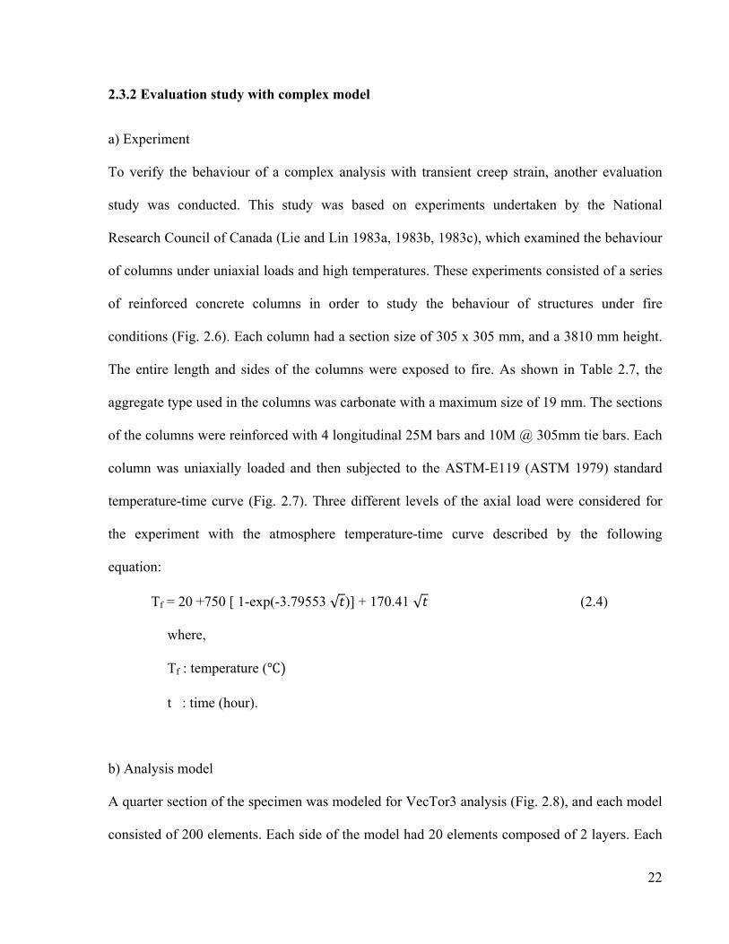
2.3.2 Evaluation study with complex model

a) Experiment

To verify the behaviour of a complex analysis with transient creep strain, another evaluation

study was conducted. This study was based on experiments undertaken by the National

Research Council of Canada (Lie and Lin 1983a, 1983b, 1983c), which examined the behaviour

of columns under uniaxial loads and high temperatures. These experiments consisted of a series

of reinforced concrete columns in order to study the behaviour of structures under fire

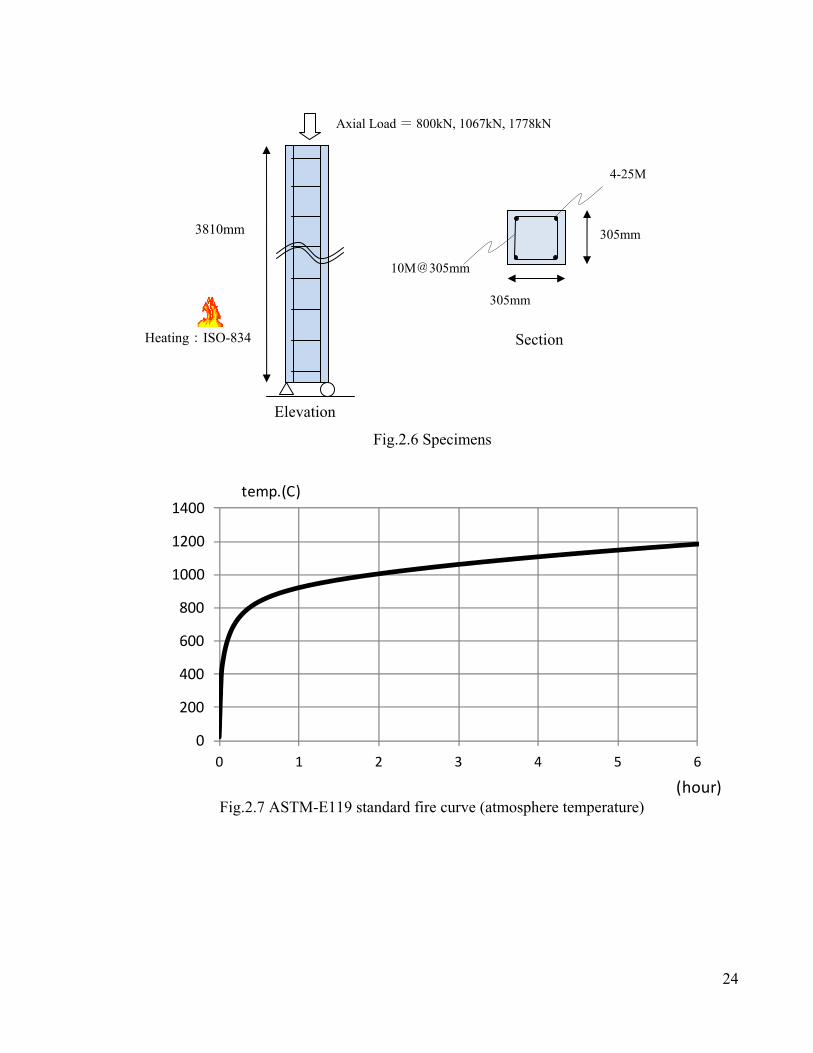
conditions (Fig. 2.6). Each column had a section size of 305 x 305 mm, and a 3810 mm height.

The entire length and sides of the columns were exposed to fire. As shown in Table 2.7, the

aggregate type used in the columns was carbonate with a maximum size of 19 mm. The sections

of the columns were reinforced with 4 longitudinal 25M bars and 10M @ 305mm tie bars. Each

column was uniaxially loaded and then subjected to the ASTM-E119 (ASTM 1979) standard

temperature-time curve (Fig. 2.7). Three different levels of the axial load were considered for

the experiment with the atmosphere temperature-time curve described by the following

equation:

Tf = 20 +750 [ 1-exp(-3.79553 √ )] + 170.41 √ (2.4)

where,

Tf : temperature (℃)

t : time (hour).

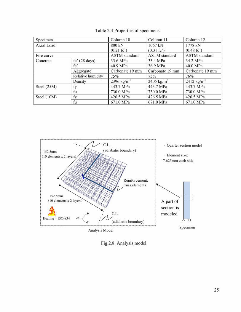
b) Analysis model

A quarter section of the specimen was modeled for VecTor3 analysis (Fig. 2.8), and each model

consisted of 200 elements. Each side of the model had 20 elements composed of 2 layers. Each

23

centreline was set as the adiabatic boundary condition for the heat transfer analysis, as well as

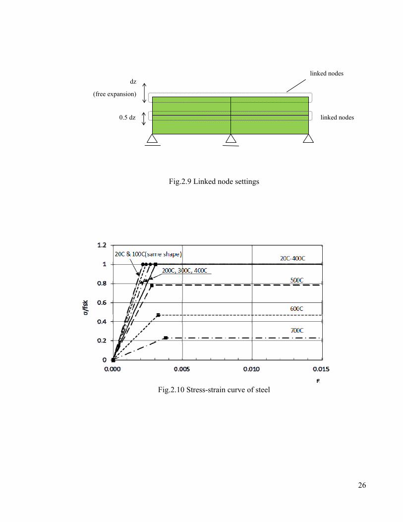
the symmetry boundary condition for the stress analysis. The reinforcement within the specimen

was modeled with truss elements. Each node of the surface of the model was set as a linked

node, and the displacement of the nodes at the middle section was restrained as 0.5 of the

displacement of the surface (Fig. 2.9). This modeling methodology was based on the assumption

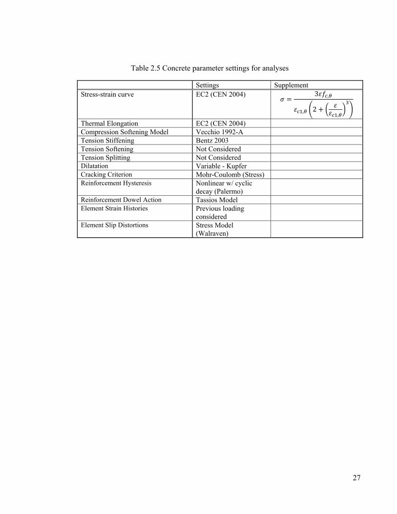
that any section of the column expands equally. Table 2.4 and Table 2.5 show the properties of

the specimens, which were also set as the parameters of the analysis model. A bilinear model

was selected for the stress-strain relationship of the steel reinforcement as shown in Fig. 2.10.

The degradation of the materials was also considered according to Eurocode2 (CEN 2004; CEN

2005), as illustrated in Table 2.6. The minimum values were set to avoid instability of analysis

caused by zero-valued components of the stiffness matrices.

In the heat transfer analysis conducted, the ASTM-E119 (ASTM 1979) standard fire curve was

used as define the atmosphere temperature, and thermal radiation and convection were also

considered acting on the surface of the model. Thermal dependencies of the thermo-physical

properties of the concrete material were set as defined by Eurocode2 (CEN 2004) (Table 2.7).

Taking the relative humidity of the concrete as 75%, the moisture content of the specimen was

assumed to be 3% to 5% (Miura, Itatani, Hakamaya 2007). Thus, the specific heat of the

concrete was calculated on the basis of two types of moisture content: 3% and 5%.

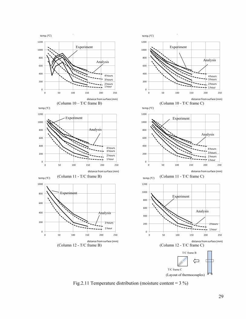
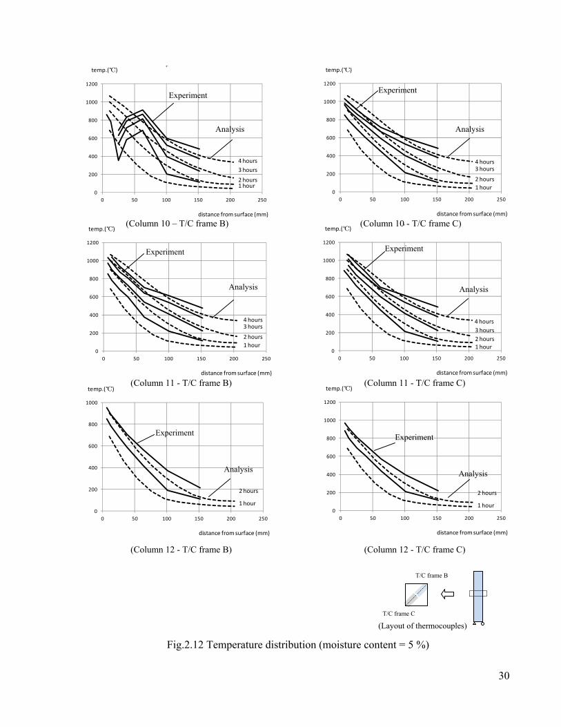
Fig 2.11 and Fig 2.12 illustrate the results of the heat transfer analysis. In general, the analysis

data and the experimental data agree at each time period. Therefore, execution of stress analysis

on the basis of these element temperatures can be regarded as reliable.

24

Fig.2.7 ASTM-E119 standard fire curve (atmosphere temperature)

0

200

400

600

800

1000

1200

1400

0 1 2 3 4 5 6

temp.(C)

(hour)

3810mm

305mm

305mm

Section

Elevation

Axial Load ＝ 800kN, 1067kN, 1778kN

4-25M

10M＠305mm

Fig.2.6 Specimens

Heating：ISO-834

25

Table 2.4 Properties of specimens

Specimen Column 10 Column 11 Column 12 Axial Load 800 kN

(0.21 fc’) 1067 kN (0.31 fc’)

1778 kN (0.48 fc’)

Fire curve ASTM standard ASTM standard ASTM standard Concrete fc’ (28 days) 33.6 MPa 33.4 MPa 34.2 MPa

fc’ 40.9 MPa 36.9 MPa 40.0 MPa Aggregate Carbonate 19 mm Carbonate 19 mm Carbonate 19 mm Relative humidity 75% 75% 76% Density 2396 kg/m3 2405 kg/m3 2412 kg/m3

Steel (25M) fy 443.7 MPa 443.7 MPa 443.7 MPa fu 730.0 MPa 730.0 MPa 730.0 MPa

Steel (10M) fy 426.5 MPa 426.5 MPa 426.5 MPa fu 671.0 MPa 671.0 MPa 671.0 MPa

C.L.

(adiabatic boundary)

152.5mm （10 elements x 2 layers）

Fig.2.8. Analysis model

Reinforcement: truss elements

Heating：ISO-834

・Quarter section model

・Element size:

7.625mm each side

A part of section is modeled

Analysis Model

152.5mm （10 elements x 2 layers）

C.L.

(adiabatic boundary)

Specimen

26

Fig.2.10 Stress-strain curve of steel

linked nodes dz

(free expansion)

0.5 dz linked nodes

Fig.2.9 Linked node settings

27

Table 2.5 Concrete parameter settings for analyses

Settings Supplement Stress-strain curve EC2 (CEN 2004) = 3 ,

, 2 + ,

Thermal Elongation EC2 (CEN 2004) Compression Softening Model Vecchio 1992-A Tension Stiffening Bentz 2003 Tension Softening Not Considered Tension Splitting Not Considered Dilatation Variable - Kupfer Cracking Criterion Mohr-Coulomb (Stress) Reinforcement Hysteresis Nonlinear w/ cyclic

decay (Palermo)

Reinforcement Dowel Action Tassios Model Element Strain Histories Previous loading

considered

Element Slip Distortions Stress Model (Walraven)

28

Table 2.6 Degradation of materials (CEN 2004 and CEN 2005)

(for stability of the analysis, actually set as 1.0e-6)

Table 2.7 Parameter settings for heat transfer analyses

Concrete (carbonate) Steel temp.(℃) fc,q/fck ε c1,θ εcu1,q Es,θ/Es fsy,θ/fyk

20 1.00 0.0025 0.0200 1.000 1.000 100 1.00 0.0040 0.0225 1.000 1.000 200 0.97 0.0055 0.0250 0.900 1.000 300 0.91 0.0070 0.0275 0.800 1.000 400 0.85 0.0100 0.0300 0.700 1.000 500 0.74 0.0150 0.0325 0.600 0.780 600 0.60 0.0250 0.0350 0.310 0.470 700 0.43 0.0250 0.0375 0.130 0.230 800 0.27 0.0250 0.0400 0.090 0.110 900 0.15 0.0250 0.0425 0.068 0.060

1000 0.06 0.0250 0.0450 0.045 0.040 1100 0.02 0.0250 0.0475 0.023 0.020 1200 0.00 - - 0.000 0.000

Settings Supplement Concrete thermal expansion EC2 (CEN 2004) carbonate aggregates Concrete Density EC2 (CEN 2004) Concrete Conductivity EC2 (CEN 2004) Concrete Specific Heat EC2 (CEN 2004) moisture content:

3% (Cp=2020 J/kg K) 5% (Cp=3250 J/kg K)

29

0

200

400

600

800

1000

1200

0 50 100 150 200 250

ptemp.(℃)

distance from surface (mm)

2 hours

1 hour0

200

400

600

800

1000

0 50 100 150 200 250

ptemp.(℃)

distance from surface (mm)

2 hours

1 hour

0

200

400

600

800

1000

1200

0 50 100 150 200 250

ptemp.(℃)

distance from surface (mm)

3 hours2 hours1 hour

4 hours

0

200

400

600

800

1000

1200

0 50 100 150 200 250

temp.(℃)

distance from surface (mm)

4 hours3 hours

2 hours1 hour

0

200

400

600

800

1000

1200

0 50 100 150 200 250

p

distance from surface (mm)

temp.(℃)

4 hours3 hours2 hours1 hour

0

200

400

600

800

1000

1200

0 50 100 150 200 250

ptemp.(℃)

distance from surface (mm)

4 hours3 hours

2 hours1 hour

(Column 10 – T/C frame B) (Column 10 - T/C frame C)

(Column 11 - T/C frame B) (Column 11 - T/C frame C)

(Column 12 - T/C frame B) (Column 12 - T/C frame C)

T/C frame B

T/C frame C

(Layout of thermocouples)

Fig.2.11 Temperature distribution (moisture content = 3 %)

Experiment

Analysis Analysis

Experiment

Experiment

Analysis Analysis

Experiment

Experiment

Analysis Analysis

Experiment

30

0

200

400

600

800

1000

1200

0 50 100 150 200 250

temp.(℃)

distance from surface (mm)

2 hours

1 hour0

200

400

600

800

1000

0 50 100 150 200 250

temp.(℃)

distance from surface (mm)

2 hours

1 hour

0

200

400

600

800

1000

1200

0 50 100 150 200 250

Temperature Distributiontemp.(℃)

distance from surface (mm)

3 hours2 hours1 hour

4 hours

0

200

400

600

800

1000

1200

0 50 100 150 200 250

Temperature Distributiontemp.(℃)

distance from surface (mm)

4 hours3 hours

2 hours1 hour

0

200

400

600

800

1000

1200

0 50 100 150 200 250

temp.(℃)

distance from surface (mm)

4 hours3 hours

2 hours1 hour

0

200

400

600

800

1000

1200

0 50 100 150 200 250

p

distance from surface (mm)

temp.(℃)

4 hours3 hours2 hours1 hour

(Column 10 – T/C frame B) (Column 10 - T/C frame C)

Experiment

Analysis Analysis

Experiment

(Column 11 - T/C frame B) (Column 11 - T/C frame C)

(Column 12 - T/C frame B) (Column 12 - T/C frame C)

Analysis

Experiment

Analysis

Experiment

Analysis

Experiment

Analysis

Experiment

T/C frame B

T/C frame C

(Layout of thermocouples)

Fig.2.12 Temperature distribution (moisture content = 5 %)

31

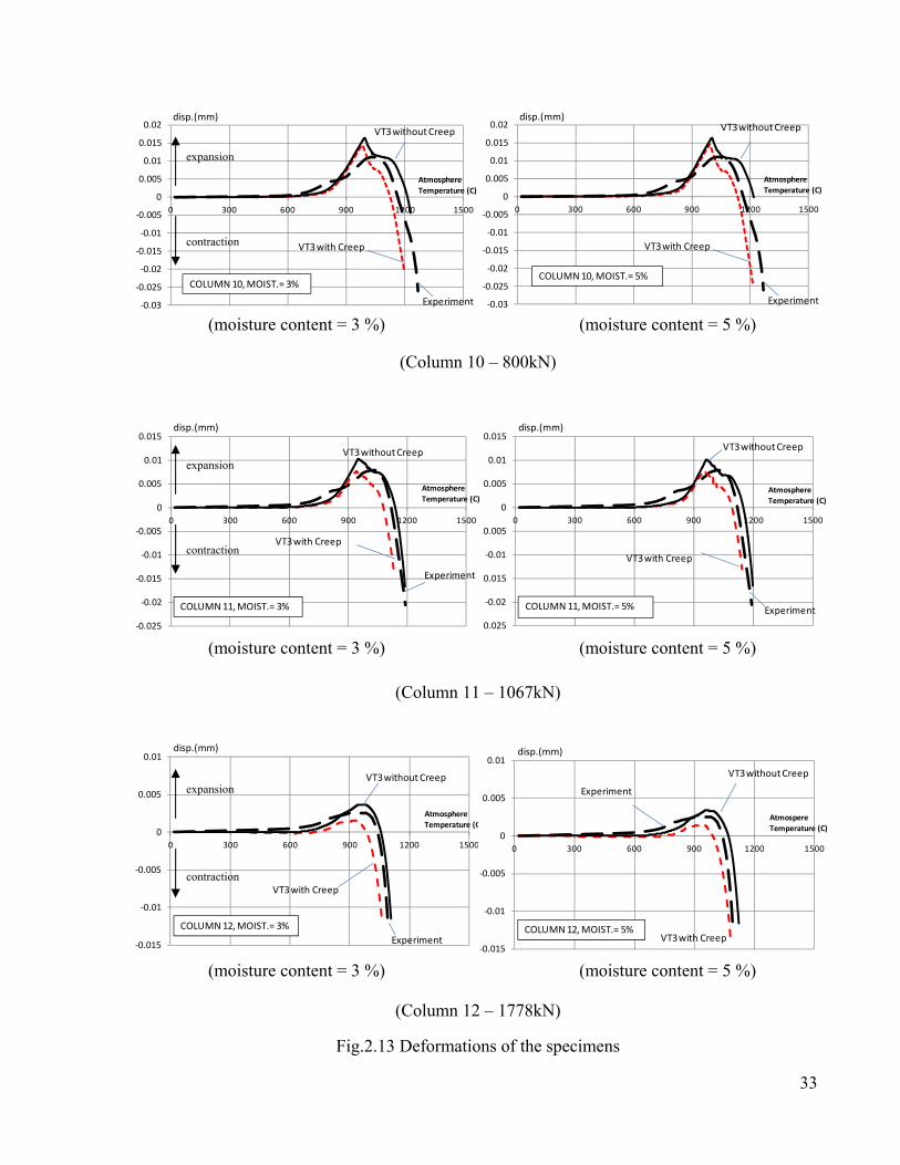
c) Results of the analyses

On the basis of the heat transfer analyses, two types of stress analyses were carried out: an

analysis without transient creep strain considered, and an analysis with transient creep strain

included. Fig. 2.13 shows the deformation of the column obtained from the stress analysis.

Because the model was one part of the column, the total deformation of the column was

calculated on the assumption that any section of the column expanded equally. As shown in the

figure, there was little difference between these two analyses in the expansion phase. However,

in the contraction phase of the column, these two graphs showed significant difference: the

deformation without the transient creep strain formed a small contraction; the deformation with

the transient creep strain showed a large contraction. Moreover, Fig. 2.13 indicates that

differences in the moisture content made only a small difference in the deformation of the

concrete (Note: In Fig. 2.13, a positive strain indicates expansion; a negative strain indicates

contraction). These results suggest that employing Gernay's definition (2012) of the transient

creep strain can lead to good predictions of the contraction phase of concrete. However, further

investigations of the transient creep strain are required to draw a firm conclusion.

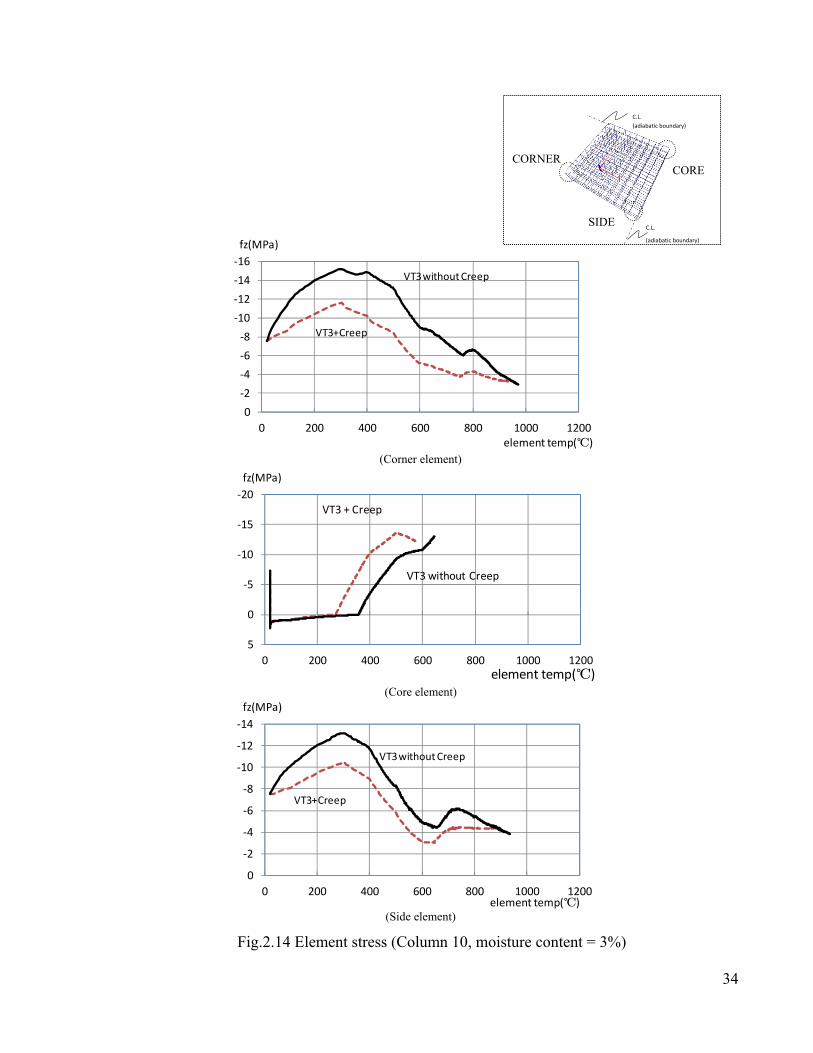
A comparison of the element stress between the analysis with transient creep strain and the

analysis without the transient creep strain is shown in Fig. 2.14. Although the deformation

graphs exhibited only a small difference, these graphs exhibit considerably different behaviour.

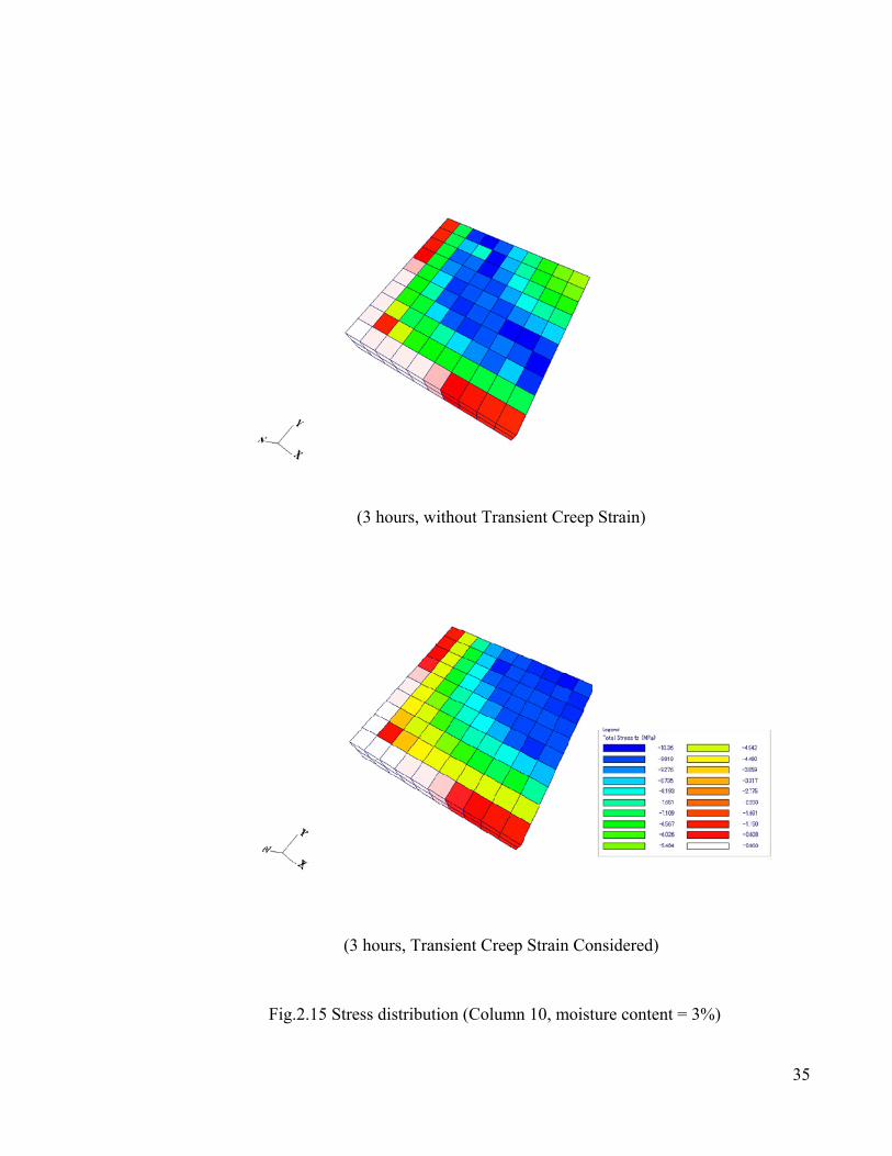
Most notable, the stress at the core element shows a higher stress when transient creep strain is

considered. Fig. 2.15 also explains these phenomena. The contours in this figure illustrate the

stress distribution determined from the analysis model at 3 hours. The two analyses indicated

different distribution patterns. The analysis with transient creep strain exhibited higher stress

32

levels at the centre of the section; meanwhile, the analysis without transient creep strain shows

lower stress levels at the centre. These results represent important implications for developing

new findings for the stress, strain or integrity of concrete structures under high temperatures.

33

Fig.2.13 Deformations of the specimens

(Column 10 – 800kN)

(Column 11 – 1067kN)

(Column 12 – 1778kN)

-0.03

-0.025

-0.02

-0.015

-0.01

-0.005

0

0.005

0.01

0.015

0.02

0 300 600 900 1200 1500

Atmosphere Temperature (C)

VT3 without Creep

VT3with Creep

Experiment

disp.(mm)

COLUMN 10, MOIST.= 3%

(moisture content = 3 %) (moisture content = 5 %)-0.03

-0.025

-0.02

-0.015

-0.01

-0.005

0

0.005

0.01

0.015

0.02

0 300 600 900 1200 1500

Atmosphere Temperature (C)

VT3 without Creep

VT3with Creep

Experiment

disp.(mm)

COLUMN 10, MOIST.= 5%

(moisture content = 3 %) (moisture content = 5 %)

-0.025

-0.02

-0.015

-0.01

-0.005

0

0.005

0.01

0.015

0 300 600 900 1200 1500

AtmosphereTemperature (C)

VT3 without Creep

VT3with Creep

Experiment

disp.(mm)

COLUMN 11, MOIST.= 5%

-0.025

-0.02

-0.015

-0.01

-0.005

0

0.005

0.01

0.015

0 300 600 900 1200 1500

Atmosphere Temperature (C)

VT3 without Creep

VT3with Creep

Experiment

disp.(mm)

COLUMN 11, MOIST.= 3%

-0.015

-0.01

-0.005

0

0.005

0.01

0 300 600 900 1200 1500

AtmosphereTemperature (C)

VT3 without Creep

VT3with Creep

Experiment

disp.(mm)

COLUMN 12, MOIST.= 3%

(moisture content = 3 %) (moisture content = 5 %)-0.015

-0.01

-0.005

0

0.005

0.01

0 300 600 900 1200 1500

Atmospere Temperature (C)

VT3 without Creep

VT3with Creep

Experiment

disp.(mm)

COLUMN 12, MOIST.= 5%

expansion

contraction

expansion

contraction

expansion

contraction

34

-14

-12

-10

-8

-6

-4

-2

00 200 400 600 800 1000 1200

element temp(℃)

fz(MPa)

VT3+Creep

VT3without Creep

Fig.2.14 Element stress (Column 10, moisture content = 3%)

-16-14-12-10

-8-6-4-20

0 200 400 600 800 1000 1200element temp(℃)

fz(MPa)

VT3+Creep

VT3 without Creep

-20

-15

-10

-5

0

50 200 400 600 800 1000 1200

element temp(℃)

fz(MPa)

VT3 + Creep

VT3 without Creep

(Corner element)

(Core element)

(Side element)

C.L.

(adiabatic boundary)

C.L. (adiabatic boundary)

CORE

SIDE

CORNER

35

Fig.2.15 Stress distribution (Column 10, moisture content = 3%)

(3 hours, Transient Creep Strain Considered)

(3 hours, without Transient Creep Strain)

36

2.4 Summary

In conclusion, as indicated in the results shown, this study reveals that VecTor3 now has the

ability to carry out analyses considering transient creep strain with good predictions of the

deformation of concrete structures under elevated temperatures. Moreover, the analyses results

point to significant differences in the stress distribution within the column sections, when

transient creep is considered. The differences in the computed behaviour suggest that new

insights can be achieved with investigations using this program.

37

CHAPTER 3: Modification of JANUS

3.1 Introduction

As discussed in Chapter 2, a new feature of VecTor3, the consideration of transient creep strain,

was developed, and its behaviour was confirmed through several analyses. In order to support

these new analysis capabilities and provide temperature and stress outputs for VecTor3, new

functions within the post-processor for VecTor were developed. Thus, this combination of

VecTor and its postprocessor (JANUS) will help users to execute their research more efficiently.

This chapter discusses the methodology and features of the newly implemented functions within

the post-processor JANUS.

3.1.1 Background

JANUS can process the output files of the VecTor programs, and it can also exhibit contours

and graphs of stresses, strains, deformations and other variables. Post-processor programs have

been developed at the University of Toronto for several years. For example, Augustus is one of

the available programs that support building, assembling and post-processing the models of

NLFEA programs (Vecchio, Bentz, Collins 2004). Although Augustus is a highly sophisticated

graphics-based post-processor, it can only handle two-dimensional (2D) analyses when used

with the VecTor programs. Therefore, there was a need to expand its ability or to develop a new

program that can process three-dimensional (3D) analyses. JANUS fits this requirement.

JANUS has been developed to provide a practical 3D graphic tool for engineers and researchers

who carry out advanced and complicated NLFEA simulations. The program processes the

output of the VecTor programs for beam sections, 2D membrane structures, 3D solid structures,

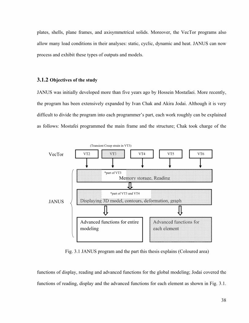
38

plates, shells, plane frames, and axisymmetrical solids. Moreover, the VecTor programs also

allow many load conditions in their analyses: static, cyclic, dynamic and heat. JANUS can now

process and exhibit these types of outputs and models.

3.1.2 Objectives of the study

JANUS was initially developed more than five years ago by Hossein Mostafaei. More recently,

the program has been extensively expanded by Ivan Chak and Akira Jodai. Although it is very

difficult to divide the program into each programmer’s part, each work roughly can be explained

as follows: Mostafei programmed the main frame and the structure; Chak took charge of the

functions of display, reading and advanced functions for the global modeling; Jodai covered the

functions of reading, display and the advanced functions for each element as shown in Fig. 3.1.

Memory storage, Reading

Displaying 3D model, contours, deformation, graph

VT2 VT3 VT4 VT5 VT6

Advanced functions for each element

Advanced functions for entire modeling

*part of VT3 and VT4

(Transient Creep strain in VT3)

VecTor

JANUS

Fig. 3.1 JANUS program and the part this thesis explains (Coloured area)

*part of VT3

39

Thus, this section discusses refinements made relating the data reading process, contour plots,

graphs, element attributes, and expansion of readable VecTor output formats. Specifically, this

chapter describes the functions, structure and features of the program as follows:

-the development environment, structure and architecture of JANUS,

-basic functions of JANUS,

-new features for VecTor2 to VecTor6,

-graph functions,

-element attributes and pick-up functions, and

-accommodations for old and new formats of output files.

40

3.2 Development environment and architecture

3.2.1 Development environment

JANUS is formulated in the Visual C++ 6.0 (VC6) environment. VC6 is one of the more

popular development tools for Windows software, and is able to handle Microsoft Foundation

Class Libraries 6.0 (MFC 6.0) as well as a standard object-oriented programming language,

C++.

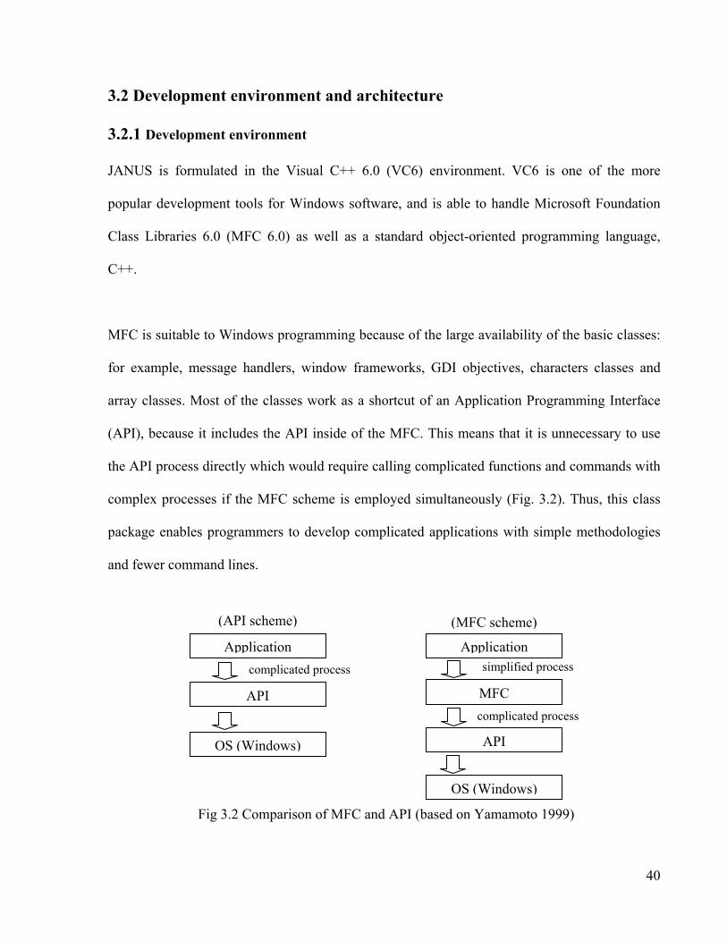
MFC is suitable to Windows programming because of the large availability of the basic classes:

for example, message handlers, window frameworks, GDI objectives, characters classes and

array classes. Most of the classes work as a shortcut of an Application Programming Interface

(API), because it includes the API inside of the MFC. This means that it is unnecessary to use

the API process directly which would require calling complicated functions and commands with

complex processes if the MFC scheme is employed simultaneously (Fig. 3.2). Thus, this class

package enables programmers to develop complicated applications with simple methodologies

and fewer command lines.

Application

API

Application

MFC

API

OS (Windows)

OS (Windows)

complicated process simplified process

complicated process

Fig 3.2 Comparison of MFC and API (based on Yamamoto 1999)

(MFC scheme) (API scheme)

41

VC6 with MFC enables developers to use the Multiple Document Interface (MDI) method,

which can manage several documents and windows at the same time. This method is preferable

for the development of JANUS, because the application needs to handle several output files and

graphic interfaces simultaneously. For instance, if JANUS is required to compare VecTor3 and

VecTor2 outputs, the MDI method that can handle two data sets at once is obviously a better

solution than the single document interface method.

An object-oriented language can manage several windows frames and documentations in

JANUS as independent objects simultaneously, so C++ is preferable for MDI applications rather

than structured programming languages. Therefore, for the reasons discussed, JANUS was built

using the VC6 environment.

3.2.2 Open GL

OpenGL is another important scheme of JANUS that manages 3D graphic interfaces. OpenGL

is one of the popular APIs that provides 2D and 3D computer graphics tools for many

applications, such as CAD programs. Moreover, OpenGL is an open resource library that works

independently from operating systems, so JANUS takes advantage of this API library, which

provides a large number of commands to support rendering, transforming and other

manipulations of graphics in fast speed.

3.2.3 Structure and architecture of JANUS

JANUS consists of a number of classes that represent the functions and resources in the

application such as windows, dialog boxes and data arrays. Although there are more than 100

42

classes utilized within the application, the most important classes among them are CDataIn,

CMesh3d, CArray, CVecHomDoc and CVecHomView. These classes are the core classes of

JANUS that are utilized whenever new output data are processed, and many other classes are

invoked to define data types or to receive the objects and the variables generated by those core

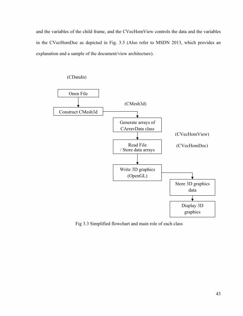
classes. Each core class has an important role as discussed in the following text.

The CDataIn class has many reading functions to open, read and close output files, and therefore

this class works as the main control for processing output data. These data also construct the

CMesh3d class in order to store output data arrays. The CMesh3d manages a number of data

arrays and OpenGL functions that are essential in drawing 3D graphics and graphs, as shown in

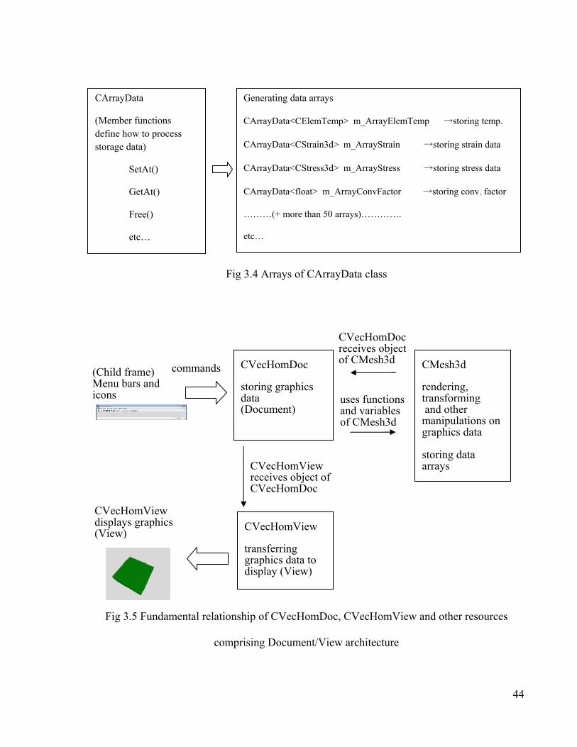
Fig. 3.3. Most of the data arrays are generated from the CArrayData class, which has

fundamental functions to control storage data, such as reading, writing and removing data. In

order to accommodate the different formats of the output files of VecTor, each data array has

suitable variables and functions for the format. These functions are defined as data types set by

the programmers of JANUS. For instance, one of these data arrays, m_ArrayElemTemp is an

array of the CArrayData class, and this array is defined by the data type CElemTemp. The

CElemTemp has the variable m_Temp to store the temperature output of each element as

illustrated in Fig. 3.4. Another array of CArrayData class for storing strain data, m_ArrayStrain,

is defined by the data type CStrain3d, which has 7 arrays.

The CVecHomDoc and the CVecHomView classes control the view and the view data that must

be generated when an output data set is read. These two classes comprise the document/view

architecture that supports the MDI application, JANUS. The CVecHomDoc manages the data

43

and the variables of the child frame, and the CVecHomView controls the data and the variables

in the CVecHomDoc as depicted in Fig. 3.5 (Also refer to MSDN 2013, which provides an

explanation and a sample of the document/view architecture).

(CDataIn)

Open File

Construct CMesh3d

Generate arrays of CArrayData class

Read File / Store data arrays

Write 3D graphics (OpenGL)

Display 3D graphics

Store 3D graphics data

(CMesh3d)

(CVecHomView)

(CVecHomDoc)

Fig 3.3 Simplified flowchart and main role of each class

44

(Child frame) Menu bars and icons

commands

CVecHomView receives object of CVecHomDoc

Fig 3.5 Fundamental relationship of CVecHomDoc, CVecHomView and other resources

comprising Document/View architecture

CMesh3d

rendering, transforming and other manipulations on graphics data storing data arrays

CVecHomDoc

storing graphics data (Document)

CVecHomView

transferring graphics data to display (View)

uses functions and variables of CMesh3d

CVecHomDoc receives object of CMesh3d

CVecHomView displays graphics (View)

Fig 3.4 Arrays of CArrayData class

CArrayData

(Member functions define how to process storage data)

SetAt()

GetAt()

Free()

etc…

Generating data arrays

CArrayData<CElemTemp> m_ArrayElemTemp →storing temp.

CArrayData<CStrain3d> m_ArrayStrain →storing strain data

CArrayData<CStress3d> m_ArrayStress →storing stress data

CArrayData<float> m_ArrayConvFactor →storing conv. factor

………(+ more than 50 arrays)………….

etc…

45

3.3 Accommodations for VecTor series

As explained in previous sections, JANUS’ structure and architecture were initially designed by

Mostafaei, and were originally prepared for VecTor3 output and limited VecTor4 variables.

However, the VecTor suite has several programs and different output formats, and these

programs do not have proper post-processors. Therefore, JANUS has been developed as a

complete post-processor for all the VecTor series. This chapter discusses this new usage and the

architecture of the newly formulated JANUS.

3.3.1 Usage

VecTor comprises five types of programs as shown in Table. 3.1. Each program has its own

elements that have different shapes, integration points and dimensions. For this reason, the

output format of each analysis program is varied, and JANUS needs an altered process for each

format. Although the inner processes are different, the user of JANUS can neglect the difference

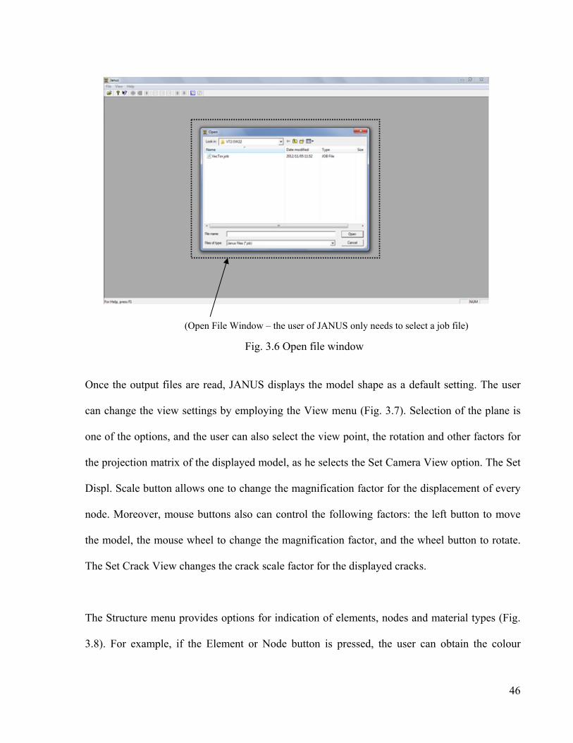
and only needs to carry out a similar operation. If the user selects a job file, JANUS reads the

format type and indicates the model and the other output results automatically (Fig. 3.6). Once

the data are read, JANUS provides many features for these formats as explained in the following

passages.

Table 3.1 Analysis type and element type

Analysis type Element Type

VecTor2 2D Quadrilateral, Triangular, Truss

VecTor3 3D solid Hexahedral, Wedge, Truss

VecTor4 3D shell 9 node shell, 6 node shell, Truss

VecTor5 2D beam Beam

VecTor6 Axisymmetric shell Quadrilateral, Triangular, Ring Bar, Truss

46

Once the output files are read, JANUS displays the model shape as a default setting. The user

can change the view settings by employing the View menu (Fig. 3.7). Selection of the plane is

one of the options, and the user can also select the view point, the rotation and other factors for

the projection matrix of the displayed model, as he selects the Set Camera View option. The Set

Displ. Scale button allows one to change the magnification factor for the displacement of every

node. Moreover, mouse buttons also can control the following factors: the left button to move

the model, the mouse wheel to change the magnification factor, and the wheel button to rotate.

The Set Crack View changes the crack scale factor for the displayed cracks.

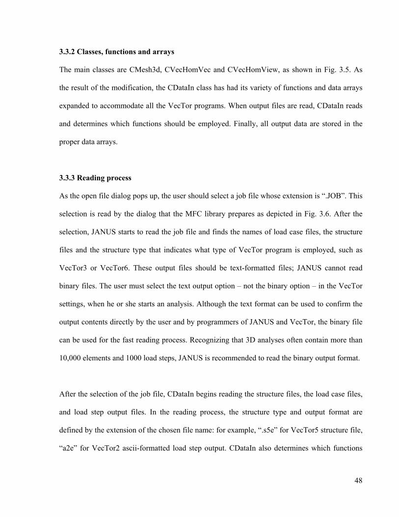
The Structure menu provides options for indication of elements, nodes and material types (Fig.

3.8). For example, if the Element or Node button is pressed, the user can obtain the colour

Fig. 3.6 Open file window

(Open File Window – the user of JANUS only needs to select a job file)

47

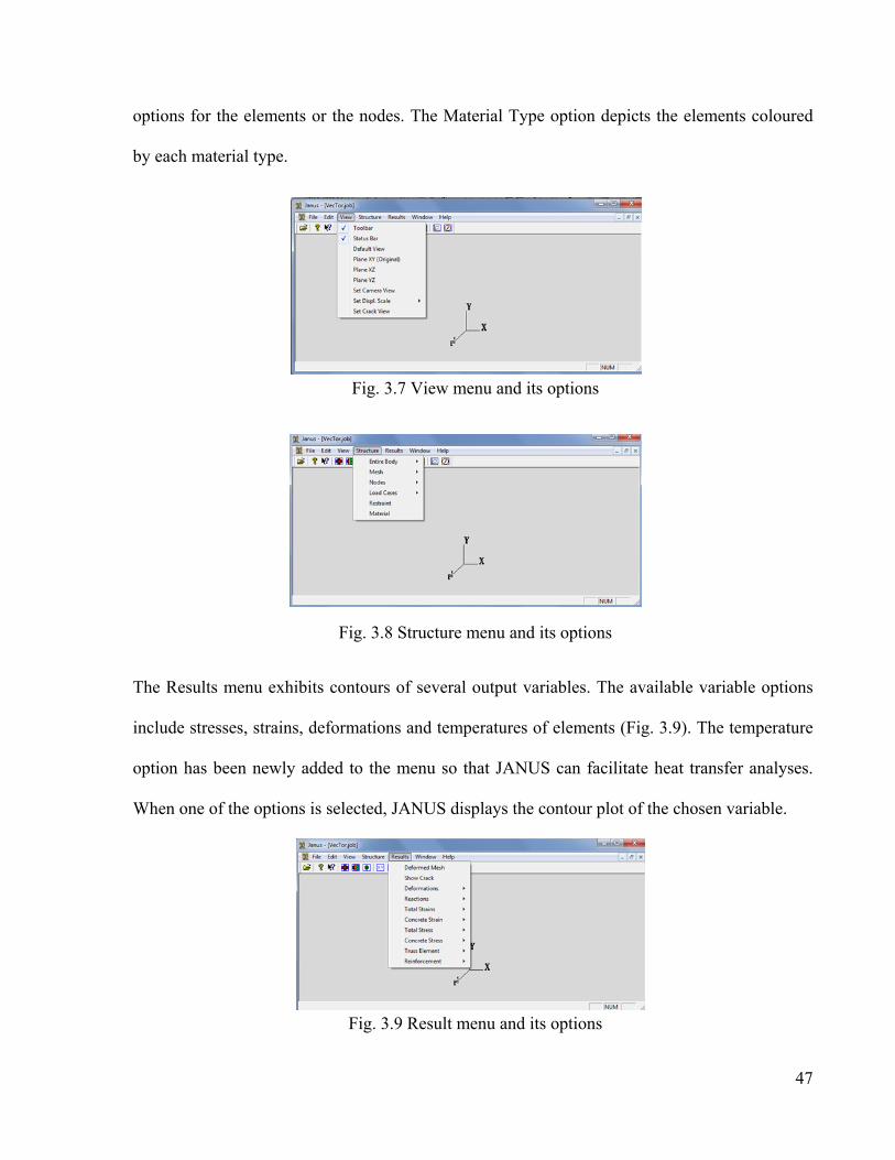
options for the elements or the nodes. The Material Type option depicts the elements coloured

by each material type.

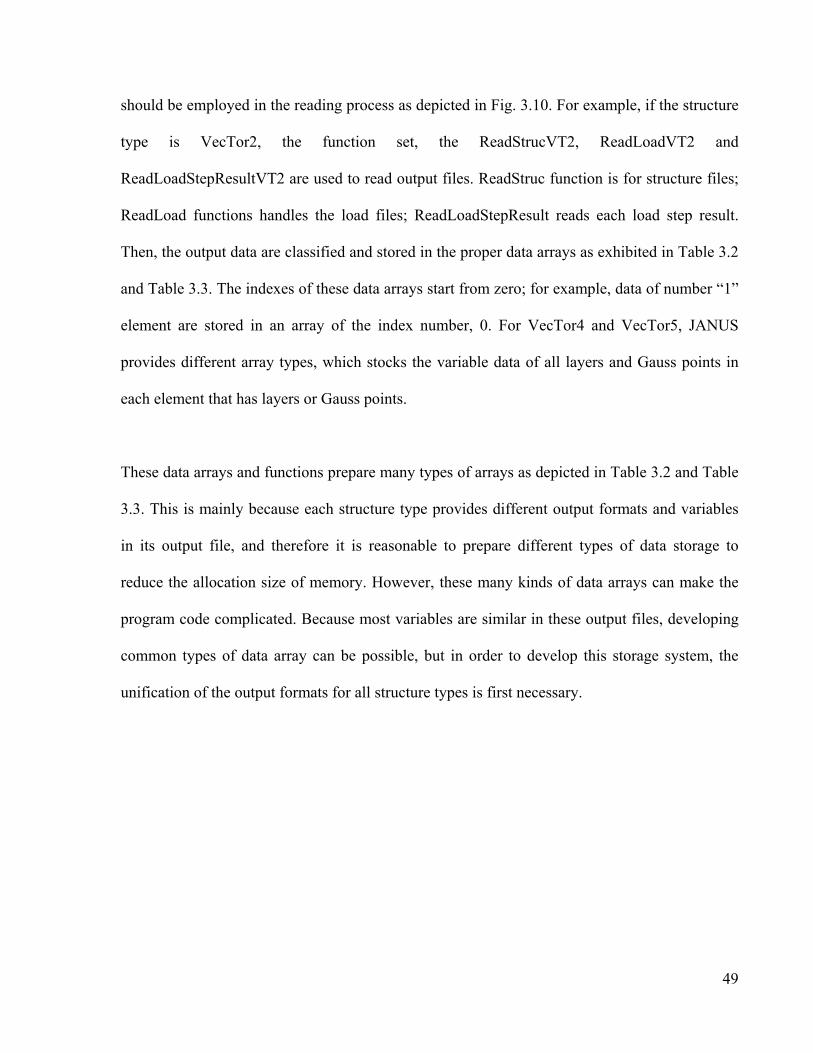
The Results menu exhibits contours of several output variables. The available variable options

include stresses, strains, deformations and temperatures of elements (Fig. 3.9). The temperature

option has been newly added to the menu so that JANUS can facilitate heat transfer analyses.

When one of the options is selected, JANUS displays the contour plot of the chosen variable.

Fig. 3.9 Result menu and its options

Fig. 3.8 Structure menu and its options

Fig. 3.7 View menu and its options

48

3.3.2 Classes, functions and arrays

The main classes are CMesh3d, CVecHomVec and CVecHomView, as shown in Fig. 3.5. As

the result of the modification, the CDataIn class has had its variety of functions and data arrays

expanded to accommodate all the VecTor programs. When output files are read, CDataIn reads

and determines which functions should be employed. Finally, all output data are stored in the

proper data arrays.

3.3.3 Reading process

As the open file dialog pops up, the user should select a job file whose extension is “.JOB”. This

selection is read by the dialog that the MFC library prepares as depicted in Fig. 3.6. After the

selection, JANUS starts to read the job file and finds the names of load case files, the structure

files and the structure type that indicates what type of VecTor program is employed, such as

VecTor3 or VecTor6. These output files should be text-formatted files; JANUS cannot read

binary files. The user must select the text output option – not the binary option – in the VecTor

settings, when he or she starts an analysis. Although the text format can be used to confirm the

output contents directly by the user and by programmers of JANUS and VecTor, the binary file

can be used for the fast reading process. Recognizing that 3D analyses often contain more than

10,000 elements and 1000 load steps, JANUS is recommended to read the binary output format.

After the selection of the job file, CDataIn begins reading the structure files, the load case files,

and load step output files. In the reading process, the structure type and output format are

defined by the extension of the chosen file name: for example, “.s5e” for VecTor5 structure file,

“a2e” for VecTor2 ascii-formatted load step output. CDataIn also determines which functions

49

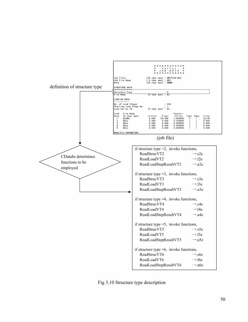
should be employed in the reading process as depicted in Fig. 3.10. For example, if the structure

type is VecTor2, the function set, the ReadStrucVT2, ReadLoadVT2 and

ReadLoadStepResultVT2 are used to read output files. ReadStruc function is for structure files;

ReadLoad functions handles the load files; ReadLoadStepResult reads each load step result.

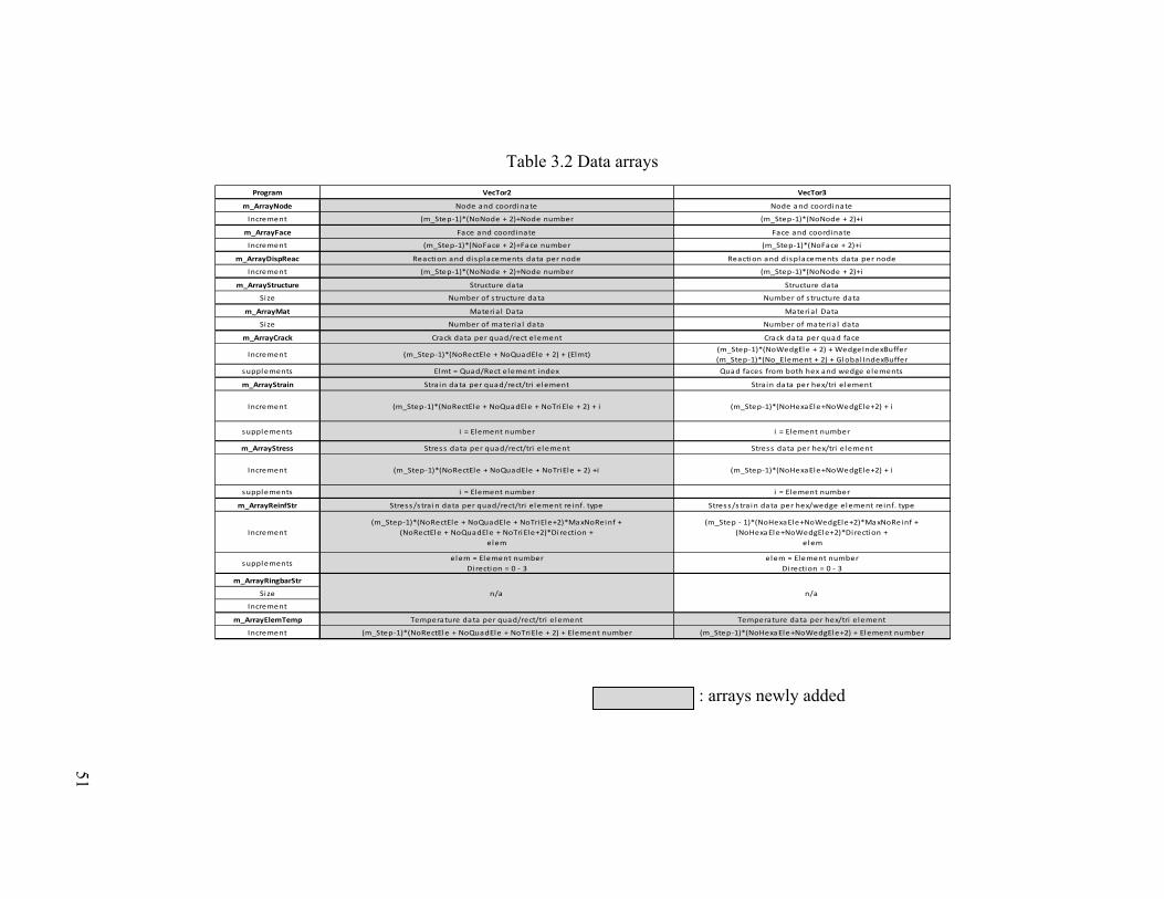
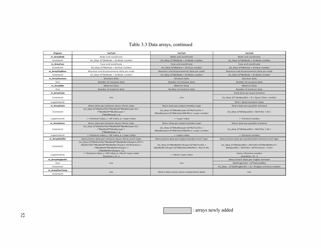
Then, the output data are classified and stored in the proper data arrays as exhibited in Table 3.2

and Table 3.3. The indexes of these data arrays start from zero; for example, data of number “1”

element are stored in an array of the index number, 0. For VecTor4 and VecTor5, JANUS

provides different array types, which stocks the variable data of all layers and Gauss points in

each element that has layers or Gauss points.

These data arrays and functions prepare many types of arrays as depicted in Table 3.2 and Table

3.3. This is mainly because each structure type provides different output formats and variables

in its output file, and therefore it is reasonable to prepare different types of data storage to

reduce the allocation size of memory. However, these many kinds of data arrays can make the

program code complicated. Because most variables are similar in these output files, developing

common types of data array can be possible, but in order to develop this storage system, the

unification of the output formats for all structure types is first necessary.

50

Fig 3.10 Structure type description

definition of structure type

(job file)

CDataIn determines functions to be employed

if structure type =2, invoke functions, ReadStrucVT2 →.s2e ReadLoadVT2 →.l2e ReadLoadStepResultVT2 →.a2e

if structure type =3, invoke functions, ReadStrucVT3 →.s3e ReadLoadVT3 →.l3e ReadLoadStepResultVT3 →.a3e

if structure type =4, invoke functions, ReadStrucVT4 →.s4e ReadLoadVT4 →.l4e ReadLoadStepResultVT4 →.a4e

if structure type =5, invoke functions, ReadStrucVT5 →.s5e ReadLoadVT5 →.l5e ReadLoadStepResultVT5 →.a5e

if structure type =6, invoke functions, ReadStrucVT6 →.s6e ReadLoadVT6 →.l6e ReadLoadStepResultVT6 →.a6e

51

Table 3.2 Data arrays

: arrays newly added

Program VecTor2 VecTor3

m_ArrayNode Node and coordinate Node and coordinate

Increment (m_Step-1)*(NoNode + 2)+Node number (m_Step-1)*(NoNode + 2)+i

m_ArrayFace Face and coordinate Face and coordinate

Increment (m_Step-1)*(NoFace + 2)+Face number (m_Step-1)*(NoFace + 2)+i

m_ArrayDispReac Reaction and displacements data per node Reaction and di splacements data per node

Increment (m_Step-1)*(NoNode + 2)+Node number (m_Step-1)*(NoNode + 2)+i

m_ArrayStructure Structure data Structure data

Size Number of s tructure data Number of structure data

m_ArrayMat Materia l Data Materia l Data

Size Number of materia l data Number of materia l data

m_ArrayCrack Crack data per quad/rect element Crack data per quad face

Increment (m_Step-1)*(NoRectEle + NoQuadEle + 2) + (Elmt)(m_Step-1)*(NoWedgEle + 2) + WedgeIndexBuffer(m_Step-1)*(No_Element + 2) + Global IndexBuffer

supplements Elmt = Quad/Rect element index Quad faces from both hex and wedge elements

m_ArrayStrain Stra in data per quad/rect/tri element Strain data per hex/tri element

Increment (m_Step-1)*(NoRectEle + NoQuadEle + NoTriEle + 2) + i (m_Step-1)*(NoHexaEle+NoWedgEle+2) + i

supplements i = Element number i = Element number

m_ArrayStress Stress data per quad/rect/tri element Stress data per hex/tri element

Increment (m_Step-1)*(NoRectEle + NoQuadEle + NoTriEle + 2) +i (m_Step-1)*(NoHexaEle+NoWedgEle+2) + i

supplements i = Element number i = Element number

m_ArrayReinfStr Stress/s tra in data per quad/rect/tri element reinf. type Stress/s train data per hex/wedge element reinf. type

Increment(m_Step-1)*(NoRectEle + NoQuadEle + NoTriEle+2)*MaxNoReinf +

(NoRectEle + NoQuadEle + NoTriEle+2)*Di rection + elem

(m_Step - 1)*(NoHexaEle+NoWedgEle+2)*MaxNoReinf + (NoHexaEle+NoWedgEle+2)*Direction +

elem

supplementselem = Element number

Direction = 0 - 3elem = Element number

Di rection = 0 - 3m_ArrayRingbarStr

Size

Increment

m_ArrayElemTemp Temperature data per quad/rect/tri element Temperature data per hex/tri element

Increment (m_Step-1)*(NoRectEle + NoQuadEle + NoTriEle + 2) + Element number (m_Step-1)*(NoHexaEle+NoWedgEle+2) + Element number

n/a n/a

52

Table 3.3 Data arrays, continued

: arrays newly added

Program VecTor4 VecTor5 VecTor6

m_ArrayNode Node and coordinate Node and coordinate Node and coordinate

Increment (m_Step-1)*(NoNode + 2)+Node number (m_Step-1)*(NoNode + 2)+Node number (m_Step-1)*(NoNode + 2)+Node number

m_ArrayFace Face and coordinate Face and coordinate Face and coordinate

Increment (m_Step-1)*(NoFace + 2)+Face number (m_Step-1)*(NoFace + 2)+Face number (m_Step-1)*(NoFace + 2)+Face number

m_ArrayDispReac Reaction and displacements data per node Reaction and displacements data per node Reaction and dis placements data per node

Increment (m_Step-1)*(NoNode + 2)+Node number (m_Step-1)*(NoNode + 2)+Node number (m_Step-1)*(NoNode + 2)+Node number

m_ArrayStructure Structure data Structure data Structure data

Size Number of s tructure data Number of s tructure data Number of s tructure data

m_ArrayMat Materia l Data Materia l Data Materia l Data

Size Number of materia l data Number of materia l data Number of materia l data

m_ArrayCrack Crack data per quad element

Increment (m_Step-1)*( NoQuadEle + 2) + Quad. Elem. number

supplements Elmt = Quad element index

m_ArrayStrain Strain data per element, Gaus s Point, layer Stra in data per output member layer Stra in data per quad/tri element

Increment(m_Step-1)*(NoShel lEle*MaxNoGP*MaxNoLayer+2) +

i*MaxNoGP*MaxNoLayer + j*MaxNoLayer + p

(m_Step-1)*(MaxNoLayer+2)*NoTrusEle + (MaxNoLayer+2)*(MemberIDBuffer) + Layer number

(m_Step-1)*(NoQuadEle + NoTriEle + 2)+ i

supplements i = Element index, j = GP index, p = Layer index i = Layer index i = Element number

m_ArrayStress Stres s data per element, Gaus s Point, layer Stress data per output member layer Stres s data per quad/tri element

Increment(m_Step-1)*(NoShel lEle*MaxNoGP*MaxNoLayer+2) +

i*MaxNoGP*MaxNoLayer + j*MaxNoLayer + p

(m_Step-1)*(MaxNoLayer+2)*NoTrusEle + (MaxNoLayer+2)*(MemberIDBuffer) + Layer number

(m_Step-1)*(NoQuadEle + NoTriEle + 2)+ i

supplements i = Element index, j = GP index, p = Layer index i = Layer index i = Element number

m_ArrayReinfStr Stress /stra in data per element, Gaus s Point, reinf. l ayer Stres s/s tra in data per output member reinf. layer Stres s/s tra in data per quad/rect/tri element reinf. type

Increment

(m_Step-1)*(NoShel lEle*MaxNoGP*MaxNoReinfLayers +2)*2 +(NoShel lEle*MaxNoGP*MaxNoReinfLayers +2)*Direction +

i*MaxNoGP*MaxNoReinfLayers + j*MaxNoReinfLayers + p;

(m_Step-1)*(MaxNoReinfLayer+2)*NoTrus Ele + (MaxNoReinfLayer+2)*(MemberIDBuffer) + Reinf. No.

(m_Step-1)*(NoQuadEle + NoTriEle+2)*MaxNoReinf +(NoQuadEle + NoTriEle +2)*Direction + elem

supplementsi = Element index, j = GP index, p = Reinf. layer index

Direction = 0 - 1i = Reinf. layer index

elem = Element numberDirection = 0 - 3

m_ArrayRingbarStr Stres s/stra in data per ringbar element

Size (NoRingbarEle + 2)*NoLoadMax

Increment (m_Step - 1)*(NoRingbarEle + 2) + Ringbar element number

m_ArrayElemTemp

Incrementn/a (Stra in data arrays s tores temperature data) n/a

n/a n/a

n/a n/a

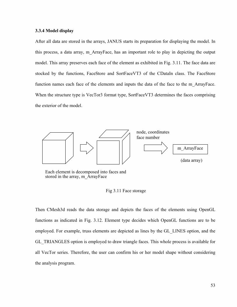
53

3.3.4 Model display

After all data are stored in the arrays, JANUS starts its preparation for displaying the model. In

this process, a data array, m_ArrayFace, has an important role to play in depicting the output

model. This array preserves each face of the element as exhibited in Fig. 3.11. The face data are

stocked by the functions, FaceStore and SortFaceVT3 of the CDataIn class. The FaceStore

function names each face of the elements and inputs the data of the face to the m_ArrayFace.

When the structure type is VecTor3 format type, SortFaceVT3 determines the faces comprising

the exterior of the model.

Then CMesh3d reads the data storage and depicts the faces of the elements using OpenGL

functions as indicated in Fig. 3.12. Element type decides which OpenGL functions are to be

employed. For example, truss elements are depicted as lines by the GL_LINES option, and the

GL_TRIANGLES option is employed to draw triangle faces. This whole process is available for

all VecTor series. Therefore, the user can confirm his or her model shape without considering

the analysis program.

Fig 3.11 Face storage

Each element is decomposed into faces and stored in the array, m_ArrayFace

m_ArrayFace

node, coordinates face number

(data array)

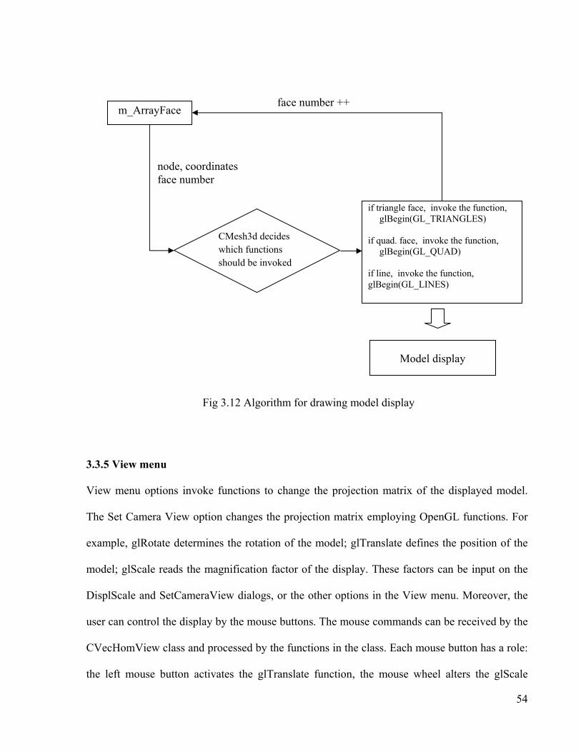
54

3.3.5 View menu

View menu options invoke functions to change the projection matrix of the displayed model.

The Set Camera View option changes the projection matrix employing OpenGL functions. For

example, glRotate determines the rotation of the model; glTranslate defines the position of the

model; glScale reads the magnification factor of the display. These factors can be input on the

DisplScale and SetCameraView dialogs, or the other options in the View menu. Moreover, the

user can control the display by the mouse buttons. The mouse commands can be received by the

CVecHomView class and processed by the functions in the class. Each mouse button has a role:

the left mouse button activates the glTranslate function, the mouse wheel alters the glScale

Fig 3.12 Algorithm for drawing model display

m_ArrayFace

node, coordinates face number

CMesh3d decides which functions should be invoked

if triangle face, invoke the function, glBegin(GL_TRIANGLES)

if quad. face, invoke the function,

glBegin(GL_QUAD) if line, invoke the function, glBegin(GL_LINES)

face number ++

Model display

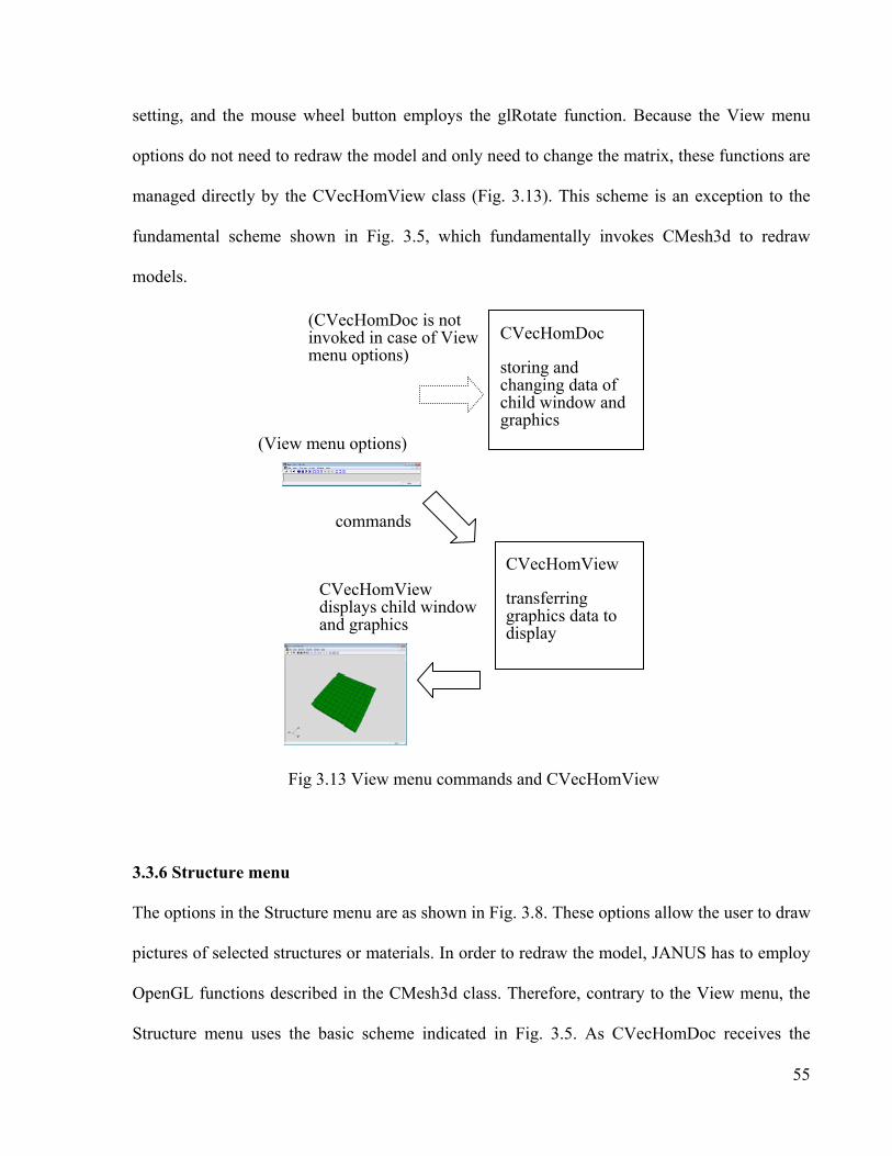
55

setting, and the mouse wheel button employs the glRotate function. Because the View menu

options do not need to redraw the model and only need to change the matrix, these functions are

managed directly by the CVecHomView class (Fig. 3.13). This scheme is an exception to the

fundamental scheme shown in Fig. 3.5, which fundamentally invokes CMesh3d to redraw

models.

3.3.6 Structure menu

The options in the Structure menu are as shown in Fig. 3.8. These options allow the user to draw

pictures of selected structures or materials. In order to redraw the model, JANUS has to employ

OpenGL functions described in the CMesh3d class. Therefore, contrary to the View menu, the

Structure menu uses the basic scheme indicated in Fig. 3.5. As CVecHomDoc receives the

(View menu options)

commands

Fig 3.13 View menu commands and CVecHomView

CVecHomDoc

storing and changing data of child window and graphics

CVecHomView

transferring graphics data to display

CVecHomView displays child window and graphics

(CVecHomDoc is not invoked in case of View menu options)

56

selection of the user, this class calls the CMesh3d to depict the model. The process of redrawing

is basically the same as the model display process; however, the employed functions are

different. CMesh3d determines which functions, elements or materials to invoke and redefines

the projection matrix. Thus, the only difference between the Structure menu and the model

display process is the selection of the functions used to draw the picture.

3.3.7 Results menu

The Results menu handles the contour options of the model. This menu uses the same scheme as

the Structure menu, which uses CVecHomDoc to receive commands and to call the CMesh3d

class. CMesh3d depicts the contour of the selected variables by the user and, in order to colour

each element, employs some OpenGL functions. The contour range is varied from white to blue,

and this colour range is defined by the glColor function. As this function changes the elements

colours, CMesh3d redraws the entire model. These options are prepared for many of the

variables (stresses, strains, displacements, and temperatures) that have been newly added.

The Results menu also has deformation options, which indicate deformations of each element as

depicted in Fig. 3.14. If this option is chosen, the CMesh3d class reads the data array,

m_ArrayDispReac and the magnification factor of the deformation that is set by the View menu.

Then CMesh3d calculates the new coordinates of each node and depicts the whole model again.

This option can be chosen independently from the contour option, so this option and the contour

display can be selected simultaneously.

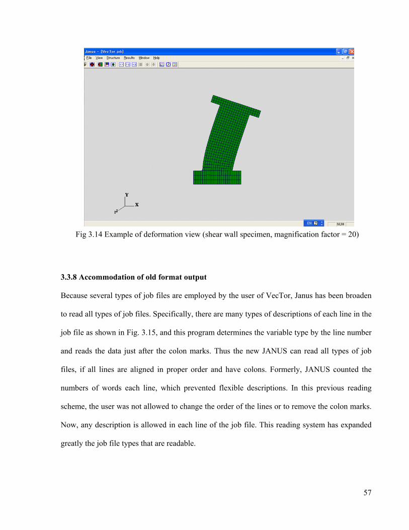
57

3.3.8 Accommodation of old format output

Because several types of job files are employed by the user of VecTor, Janus has been broaden

to read all types of job files. Specifically, there are many types of descriptions of each line in the

job file as shown in Fig. 3.15, and this program determines the variable type by the line number

and reads the data just after the colon marks. Thus the new JANUS can read all types of job

files, if all lines are aligned in proper order and have colons. Formerly, JANUS counted the

numbers of words each line, which prevented flexible descriptions. In this previous reading

scheme, the user was not allowed to change the order of the lines or to remove the colon marks.

Now, any description is allowed in each line of the job file. This reading system has expanded

greatly the job file types that are readable.

Fig 3.14 Example of deformation view (shear wall specimen, magnification factor = 20)

58

However, this reading system is only applicable to the job file. The other output types, the load

case file, the structure file and the load step result file, do not allow the free description format.

Instead, each line is determined by its head line and numbers of words. Therefore,

fundamentally, a user or programmer of VecTor should not change these output formats.

Moreover, because the format difference makes the source code very complicated, it is desirable

to consolidate these formats.

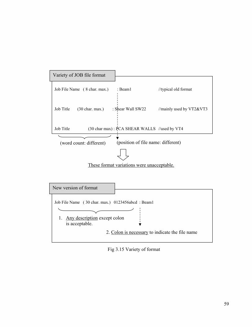
59

Job File Name ( 30 char. max.) 0123456abcd : Beam1

Fig 3.15 Variety of format

Job File Name ( 8 char. max.) : Beam1 //typical old format

Job Title (30 char. max.) : Shear Wall SW22 //mainly used by VT2&VT3

Job Title (30 char max) : PCA SHEAR WALLS //used by VT4

(position of file name: different) (word count: different)

These format variations were unacceptable.

1. Any description except colon is acceptable.

New version of format

2. Colon is necessary to indicate the file name

Variety of JOB file format

60

3.4 Element attributes indication

JANUS was modified with a new feature whereby the user can obtain attributes of an element

exhibited on the display with a simple and intuitive operation. This section discusses the usage

and the modification related to this new feature of JANUS.

3.4.1 Usage

The user of JANUS can pick any element on the displayed model, and JANUS will indicate the

element attributes immediately after the pick operation. This operation is easy, because the user

of JANUS only needs to click his right mouse buttons aiming the pointers at an element of the

displayed model. This feature is also available in the contour mode and the HotSpot mode, not

only the model display mode. Moreover, this feature does not depend on the model type, so the

user can pick up any element in either a 2D model or a 3D model. One example is shown in Fig

3.16 and Fig. 3.17. When the user chooses one element and clicks on it, JANUS opens a new

window and indicates the attributes of the element as follows: the stress, the strain, the material

type, the nodes numbers, the coordinates and the element number. The chosen element is

exhibited in a different colour so that the user can confirm which element is selected. When the

user selects the OK button on the window, the display returns to the previous mode such as the

contour, the model display or the HotSpot mode.

3.4.2 Modification and classes

Although this operation is quite simple, the resulting output is sophisticated. The program

consists of several functions to facilitate the acquisition and indication of selected element

information. In order to carry out these calculations, several classes are employed.

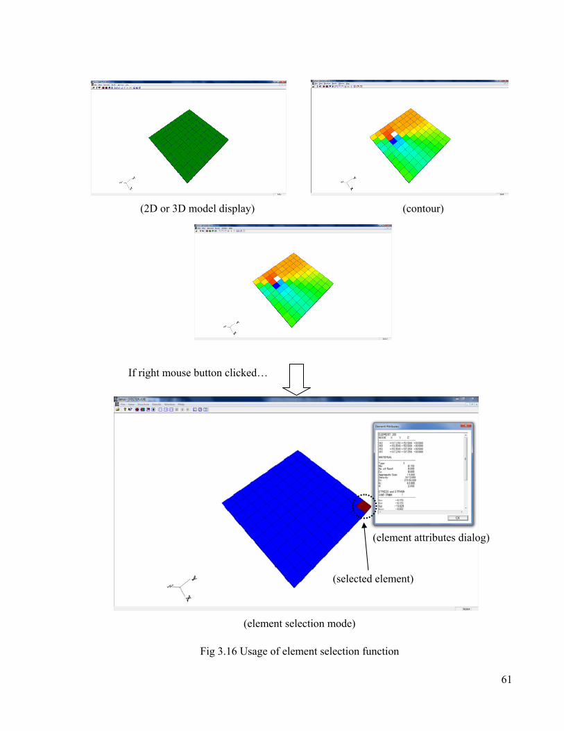
61

Fig 3.16 Usage of element selection function

(element selection mode)

(selected element)

(element attributes dialog)

(2D or 3D model display) (contour)

If right mouse button clicked…

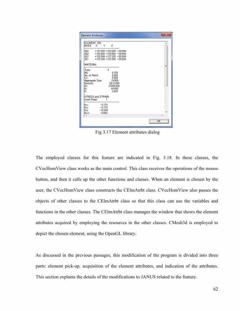
62

The employed classes for this feature are indicated in Fig. 3.18. In these classes, the

CVecHomView class works as the main control. This class receives the operations of the mouse

button, and then it calls up the other functions and classes. When an element is chosen by the

user, the CVecHomView class constructs the CElmAtrbt class. CVecHomView also passes the

objects of other classes to the CElmAtrbt class so that this class can use the variables and

functions in the other classes. The CElmAtrbt class manages the window that shows the element

attributes acquired by employing the resources in the other classes. CMesh3d is employed to

depict the chosen element, using the OpenGL library.

As discussed in the previous passages, this modification of the program is divided into three

parts: element pick-up, acquisition of the element attributes, and indication of the attributes.

This section explains the details of the modifications to JANUS related to the feature.

Fig 3.17 Element attributes dialog

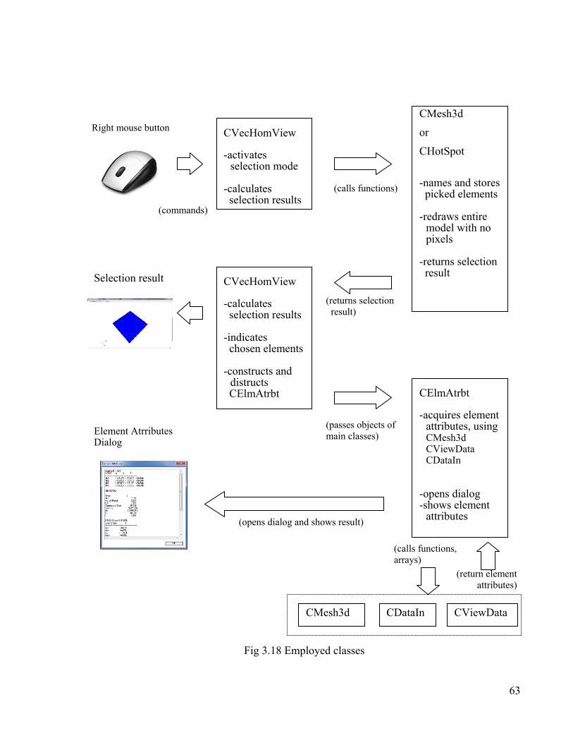
63

Fig 3.18 Employed classes

Right mouse button

(commands)

CVecHomView

-activates selection mode

-calculates selection results

Selection result

CMesh3d

or

CHotSpot

-names and stores picked elements -redraws entire

model with no pixels

-returns selection result

CVecHomView

-calculates selection results -indicates chosen elements -constructs and

distructs CElmAtrbt CElmAtrbt

-acquires element attributes, using

CMesh3d CViewData CDataIn -opens dialog -shows element

attributes

(calls functions)

Element AtrributesDialog

(returns selection result)

(passes objects of main classes)

(opens dialog and shows result)

CMesh3d CViewDataCDataIn

(return element attributes)

(calls functions, arrays)

64

3.4.3 Element pick-up

This feature is fundamentally a combination of functions in the OpenGL library. There is

another choice that employs other API libraries to calculate the closest element to a mouse

pointer, but that method was not adopted. The reason is because that method is not applicable to

3D models or requires very complicated coding, although it is beneficial for 2D models. To the

contrary, employing the OpenGL library enabled the pick-up functions for 3D models with

simple program codes. This methodology writes another invisible model on the display and

reads the elements that coincide with the mouse pointer (Fig. 3.19). As shown in Fig. 3.20, this

multi-stage method can be described in several steps as follows:

a) preparation of a selection buffer and selection mode,

b) setting projection matrix,

c) drawing elements,

d) specification of the selected element, and

e) indication of the chosen element.

a) Preparation of a selection buffer

A selection buffer is prepared to store the result of the selection process of an element. At the

beginning of the program, this buffer size is prepared, and the buffer is sent to OpenGL

functions. Next, the OpenGL mode is changed from the rendering mode to the selection mode,

which is a special mode used to select an element. The Selection mode is actually a rendering

mode, but this mode does not write any pixels.

b) Setting projection matrix

65

Second, as well as an ordinary rendering mode, the settings of the projection matrix are

adjusted. Specifically, this program reads the latest variables of the projection matrix such as the

view point, the rotation and the magnification ratio. Next, the same variables are set as the

settings of the projection matrix for the selection mode. The selection area of the mouse pointer,

which is necessary to select an element, is also adjusted simultaneously.

c) Drawing elements

As all the preparations for drawing the model are carried out, OpenGL functions start drawing

another model on the display. However, the selection mode does not write any pixels on the

screen. Simultaneously, the OpenGL names and stores the elements of the model. These

functions are as follows:

-glPopname to remove a name,

-glPushname to add a name, and

-glLoadname to overwrite the name.

This name storage OpenGL allows for arrays of numbers. For example, a name “1-2-3” or “2-1”

is also acceptable as well as “1” or “5” (Fig. 3.21 and Fig. 3.22). This format is necessary in

order to find and identify selected elements. These functions are found within the drawing

functions in the CMesh3d class and the CHotSpot class. The latest mode of the display decides

which class should be employed.

d) Specification of the selected element

When finished depicting the model with no pixel output, this program terminates the selection

mode and obtains the result. When the selection mode is terminated, OpenGL returns the

66

number of the selected elements. The result of the selection mode is also contained in the

selection buffer. The buffer holds the chosen element names and the depth values, which are

stored at Step c). This program compares each depth value to find which element is closer to the

display (Fig. 3.23). If some elements have a same depth value, this program uses the following

order of priority: point, line and face.

e) Indication of the chosen element

Finally, this program indicates the chosen element with a different color in the model so that the

user can determine which element is selected as shown in Fig. 3.19. This task is assigned to the

function, CVecHomView::PickResults. In this step, the function redraws the entire model

employing the rendering mode to indicate the chosen element in a different colour.

3.4.4 Extraction of element attributes

The selected element information is contained in the buffer, but this information relates to only a

few attributes of the element. In order to obtain the element number, the coordinates and other

important attributes, this program employs two methods. Firstly, in order to find the element

number and the element type, this program attempts to use the data arrays in other classes as

shown in Fig. 3.18. Using the face number as the reference number, this program extracts the

element type (in the HotSpot mode, this step is skipped). Secondly, this program extracts the

coordinates, the material type, and the stress and strain information. This work is mainly

assigned to the DataView function in the CElmAtrbt class. These attributes are obtained by

accessing the data arrays and the functions in the main classes. CElmAtrbt can use these other

classes’ resources, because the CVecHomView class passes the object of these main classes

67

when constructing CElmAtrbt as depicted in Fig. 3.24. The coordinates, the nodes and the

material type are obtained from the data arrays in CDataIn, and the strains and stresses are

acquired by accessing the function, Get_Variable in the CViewData.

3.4.5 Indication of element attributes

The element attributes obtained in the previous step are indicated in the dialog window of the

CElmAtrbt class. This information appears in a text format so that the user can cut and copy this

output. This window is a modal dialog window; if the user pushes the “OK” button, the dialog

disappears.

3.4.6 Indication of previous display

As the user selects the “OK” button of the dialog window and the window disappears, the

program goes back to the previous display. In this step, the CElmAtrbt class is deconstructed,

and the windows handler returns to the CVecHomView class. Then the CVecHomView class

tries to access the CMesh3d or the CHotSpot to redraw the model as displayed in the previous

mode. Thus the user can finally finish the element selection.

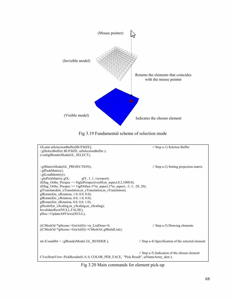
68

Fig 3.20 Main commands for element pick-up

GLuint uiSelectionBuffer[BUFSIZE]; // Step a-1) Selction Buffer ::glSelectBuffer( BUFSIZE, uiSelectionBuffer ); (void)glRenderMode(GL_SELECT); ::glMatrixMode(GL_PROJECTION); // Step a-2) Setting projection matrix ::glPushMatrix(); ::glLoadIdentity(); ::gluPickMatrix( glX, glY, 1, 1, viewport); if(flag_Ortho_Prespec == 0)gluPerspective(60,m_aspect,0.2,1000.0); if(flag_Ortho_Prespec == 1)glOrtho(-3*m_aspect,3*m_aspect, -3, 3, -20, 20); glTranslated(m_xTranslation,m_yTranslation,m_zTranslation); glRotatef(m_xRotation, 1.0, 0.0, 0.0); glRotatef(m_yRotation, 0.0, 1.0, 0.0); glRotatef(m_zRotation, 0.0, 0.0, 1.0); glScalef(m_xScaling,m_yScaling,m_zScaling); InvalidateRect(NULL,FALSE); pDoc->UpdateAllViews(NULL); ((CMesh3d *)pScene->GetAt(0))->m_ListDone=0; // Step a-3) Drawing elements ((CMesh3d *)pScene->GetAt(0))->CMesh3d::glBuildList(); int iCountHit = ::glRenderMode( GL_RENDER ); // Step a-4) Specification of the selected element // Step a-5) Indication of the chosen element CVecHomView::PickResults(0, 0, 0, COLOR_PER_FACE, "Pick Result", uiNameArray_dest );

Fig 3.19 Fundamental scheme of selection mode

(Mouse pointer)

(Invisible model)

Returns the elements that coincides with the mouse pointer

Indicates the chosen element (Visible model)

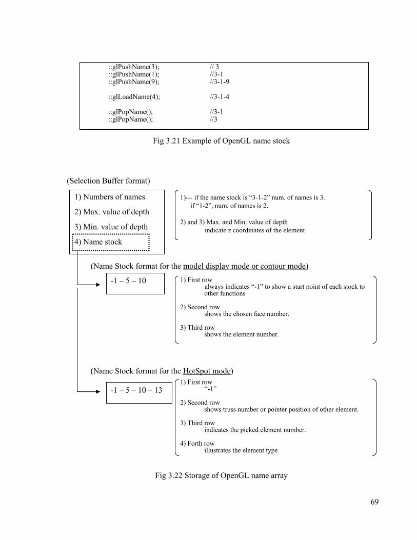
69

Fig 3.22 Storage of OpenGL name array

::glPushName(3); // 3 ::glPushName(1); //3-1 ::glPushName(9); //3-1-9 ::glLoadName(4); //3-1-4 ::glPopName(); //3-1 ::glPopName(); //3

Fig 3.21 Example of OpenGL name stock

1) Numbers of names

2) Max. value of depth

3) Min. value of depth

4) Name stock

(Selection Buffer format)

1)--- if the name stock is “3-1-2” num. of names is 3. if “1-2”, num. of names is 2. 2) and 3) Max. and Min. value of depth indicate z coordinates of the element

-1 – 5 – 10 1) First row always indicates “-1” to show a start point of each stock to other functions

2) Second row shows the chosen face number.

3) Third row shows the element number.

(Name Stock format for the model display mode or contour mode)

-1 – 5 – 10 – 13 1) First row

“-1”

2) Second row shows truss number or pointer position of other element.

3) Third row indicates the picked element number.

4) Forth row illustrates the element type.

(Name Stock format for the HotSpot mode)

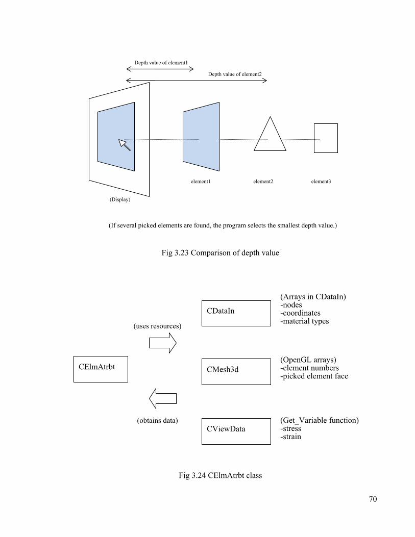
70

Fig 3.24 CElmAtrbt class

CDataIn

CMesh3d

CViewData

(Arrays in CDataIn)-nodes -coordinates -material types

(OpenGL arrays)-element numbers -picked element face

(Get_Variable function)-stress -strain

CElmAtrbt

(uses resources)

(obtains data)

Fig 3.23 Comparison of depth value

(Display)

Depth value of element1

Depth value of element2

element1 element2 element3

(If several picked elements are found, the program selects the smallest depth value.)

71

3.5 Graph and data generating functions

JANUS has had its graph and data generation functions expanded and new features added.

These functions were formerly built by Mostafaei whereby JANUS was able to generate output

of the variables and depict a graph plot. However, these functions were limited to a few

variables of VecTor3 and VecTor4 only. Moreover, the plot function was limited to one plot

with a fixed x-axis variable: load step. The graph style or design was also unchangeable. Now,

with the changes, these functions can accommodate all types of output files generated by the

VecTor series programs, with an increased number of variables available for the data selection.

In addition, JANUS can plot five variables simultaneously. Moreover, the user can change the

graph style and the plot design. This section explains and discusses these functions and the new

features of JANUS.

3.5.1 Usage

When the user of JANUS selects the plot icon, , JANUS activates a data platform window as

exhibited in Fig. 3.25. This window controls the data generating function and the graph function.

This window consists of several buttons, check boxes and input boxes that allow the user to

select all the options and variables relating to these functions. For VecTor4 and VecTor5, whose

output formats usually have layers/concrete layers and gauss points/steel layers, this program

provides appropriate input fields. The user of VecTor4 or VecTor5 can extract the output result

within the designated layer/concrete layer and gauss point/steel layer.

The Generate Data button located on the upper right position of the window is for outputting the

data arrays designated by the user. In order to select the output variables, the Variable buttons

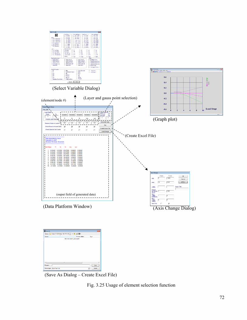
72

Fig. 3.25 Usage of element selection function

(Select Variable Dialog)

(Data Platform Window)

(Graph plot)

(Axis Change Dialog)

(Save As Dialog – Create Excel File)

(ouput field of generated data)

(Layer and gauss point selection) (element/node #)

(Create Excel File)

73

are prepared for the JANUS user. If one of the Variable buttons is chosen, the Select Variable

window appears, and the user can choose one of the variables indicated on the window. The user

can also choose the element or node numbers using the Element/Node input boxes. When the

Generate Data button is pushed, the output field shows the data arrays of the chosen variables

within the selected elements/nodes.

If the Plot button is pressed, JANUS illustrates a graph frame and plots line graphs of the

selected variables. The selection method of variables and elements/nodes is precisely the same

as the data generating process. The user can also choose which variable is to be set as the x-axis,

employing the check boxes below the element/node number boxes. Up to five variables can be

drawn on the graph area simultaneously.

The JANUS user can also customize the plot area, the axis and the tick designs of the graph. If

the user presses the Axis Change button, a new window is created to provide the set-up options

of the graph. The user can select the minimum/maximum values, the labels, the spaces between

ticks, the tick label intervals, the tick label digits, the graph titles and the auto-plot options of the

plot area. The minimum or maximum value controls the range of the plot area. The labels appear

along with the axes; the labels indicate the unit of each axis, such as “MPa” and “mm”. The

space between ticks adjusts the shape of the plot area, so the user can set up the density of major

ticks. The user also can control the frequency and the shape of the tick labels by inputting the

tick label intervals and the digits. Moreover, the graph title can be placed above the plot area.

The plot options allow the user to return anytime to the default settings of the graph: the

max/min plot range as the max/min value of the line graph and 7 ticks in each axis.

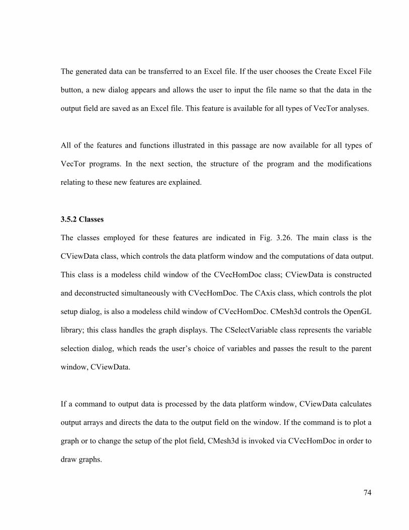
74

The generated data can be transferred to an Excel file. If the user chooses the Create Excel File

button, a new dialog appears and allows the user to input the file name so that the data in the

output field are saved as an Excel file. This feature is available for all types of VecTor analyses.

All of the features and functions illustrated in this passage are now available for all types of

VecTor programs. In the next section, the structure of the program and the modifications

relating to these new features are explained.

3.5.2 Classes

The classes employed for these features are indicated in Fig. 3.26. The main class is the

CViewData class, which controls the data platform window and the computations of data output.

This class is a modeless child window of the CVecHomDoc class; CViewData is constructed

and deconstructed simultaneously with CVecHomDoc. The CAxis class, which controls the plot

setup dialog, is also a modeless child window of CVecHomDoc. CMesh3d controls the OpenGL

library; this class handles the graph displays. The CSelectVariable class represents the variable

selection dialog, which reads the user’s choice of variables and passes the result to the parent

window, CViewData.

If a command to output data is processed by the data platform window, CViewData calculates

output arrays and directs the data to the output field on the window. If the command is to plot a

graph or to change the setup of the plot field, CMesh3d is invoked via CVecHomDoc in order to

draw graphs.

75

CMesh3d

(Plot function)

-draws graphs -alters graph

ticks, legends, labels.

Fig. 3.26 Employed classes

(passes user settings)

CSelectVariables

-obtains user’s selection

data generation results CViewData

-receives user’s commands, preferences

-calculates data array -outputs results on the

ouput field -creates Excel

files

CAxis

-obtains user’s preferences of graph settings

(invokes the plot function)

(invokes the Axis Change dialog)

CVecHomDoc

Parent class of CViewData and CAxis

(passes user settings)

(passes user settings & commands)

(returns user commands)

CDataIn

-stocks data arrays

(provides data arrays)

76

3.5.3 Data generation and graph plot

The data generating function is mainly processed by OnGenerateData in the CViewData class.

This function invokes the data arrays in the CDataIn class, which stores the output data of

VecTor programs. The data in the arrays are stored in the order defined by the analysis type and

the variable type as exhibited in Table 3.4 and Table 3.5. The OnGenerateData function reads

the arrays and returns the result to the CViewData class, and then CViewData indicates the

result on its output field.

The plot process also uses the result of the OnGenerateData function, but this process needs the

additional help of other classes and functions. After OnGenerateData output the result of its

extracting of data arrays, the plotting function CMesh3d::Plot is activated via the CVecHomDoc

class. This function draws graphs and plot fields employing the OpenGL library, which depicts

the plots, the labels and the ticks of the field as a collection of lines. Therefore, the employed

OpenGL functions are relatively simple ones (Fig. 3.27). The glBegin function defines the line

draw mode as the beginning of the drawing, and then glVertex3f determines the coordinates of

lines. The line colours are set by the glColor3f, and the line widths are controlled by

glLineWidth. These ticks and graphs are exhibited on a plane in different 3D space from the

model display, and therefore the graph view settings, such as the magnification factor and the

viewpoint, are separately fixed from the model view settings.

The ability of this plot function was expanded; now, it can plot up to five graphs on the plot

field in different colours. Formerly, only one plot line was available.

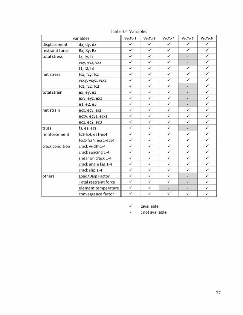
77

Table 3.4 Variables

VecTor2 VecTor3 VecTor4 VecTor5 VecTor6

displacement dx, dy, dz restraint force Rx, Ry, Rz

fx, fy, fz - vxy, vyz, vxz - f1, f2, f3 fcx, fcy, fcz vcxy, vcyz, vcxz fc1, fc2, fc3 - ex, ey, ez - exy, eyz, exz - e1, e2, e3 - ecx, ecy, ecz ecxy, ecyz, ecxz ec1, ec2, ec3

truss fs, es, ecs - fs1-fs4, es1-es4 fcs1-fcs4, ecs1-ecs4 crack width1-4 crack spacing 1-4 shear on crack 1-4 crack angle lag 1-4 crack slip 1-4 Load/Disp Factor - Total restraint force - element temperature - - convergence factor

:available- : not available

others

reinforcement

variables

total stress

net stress

total strain

net strain

crack condition

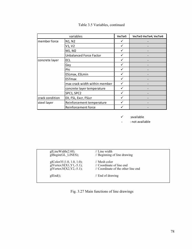
78

Table 3.5 Variables, continued

glLineWidth(2.0f); // Line width glBegin(GL_LINES); // Beginning of line drawing glColor3f (1.0, 1.0, 1.0); // Mesh color glVertex3f(X1,Y1,-5.1); // Coordinate of line end glVertex3f(X2,Y2,-5.1); // Coordinate of the other line end glEnd(); // End of drawing

Fig. 3.27 Main functions of line drawings

VecTor5 VecTor2-VecTor4, VecTor6

N1, N2 -V1, V2 -M1, M2 -Unbalanced Force Factor -ECL -Gxy -Phi -ESLmax, ESLmin -ESTmax -max crack width within member -concrete layer temperature -SPC1, SPC2 -

crack condition EX, FSL, Excr, FSLcr -Reinforcement temperature -Reinforcement force -

:available- : not available

variablesmember force

concrete layer

steel layer

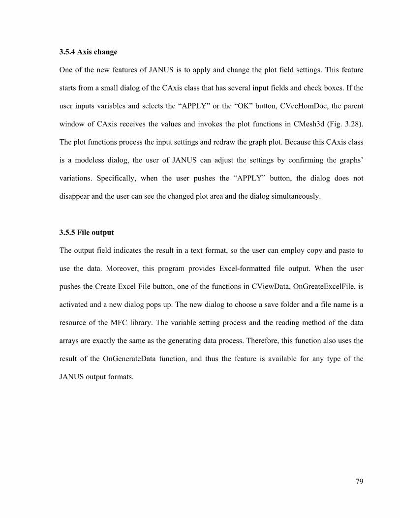
79

3.5.4 Axis change

One of the new features of JANUS is to apply and change the plot field settings. This feature

starts from a small dialog of the CAxis class that has several input fields and check boxes. If the

user inputs variables and selects the “APPLY” or the “OK” button, CVecHomDoc, the parent

window of CAxis receives the values and invokes the plot functions in CMesh3d (Fig. 3.28).

The plot functions process the input settings and redraw the graph plot. Because this CAxis class

is a modeless dialog, the user of JANUS can adjust the settings by confirming the graphs’

variations. Specifically, when the user pushes the “APPLY” button, the dialog does not

disappear and the user can see the changed plot area and the dialog simultaneously.

3.5.5 File output

The output field indicates the result in a text format, so the user can employ copy and paste to

use the data. Moreover, this program provides Excel-formatted file output. When the user

pushes the Create Excel File button, one of the functions in CViewData, OnGreateExcelFile, is

activated and a new dialog pops up. The new dialog to choose a save folder and a file name is a

resource of the MFC library. The variable setting process and the reading method of the data

arrays are exactly the same as the generating data process. Therefore, this function also uses the

result of the OnGenerateData function, and thus the feature is available for any type of the

JANUS output formats.

80

Fig. 3.28 CAxis and CVecHomDoc

CAxis

Member variables xmax, xmin, ymax, ymin, label, tickspace, ticks digits, title xmax = input1 ymax = user input2 xmin = user input3 …and same as other

variables

CVecHomDoc (parent window) -obtains the object and overwrites member variables xmax = pDlg.xmax ymax = pDlg.ymax xmin = pDlg.xmin …and same as other

variables

(passes object, pDlg)

(user input) (commands)

Axis Change dialog

(calls OnAxis function)

(calls AxisChange function) (passes member variables)

CMesh3d

AxisChange function and Plot function -alters graph ticks,

legends, labels, digits

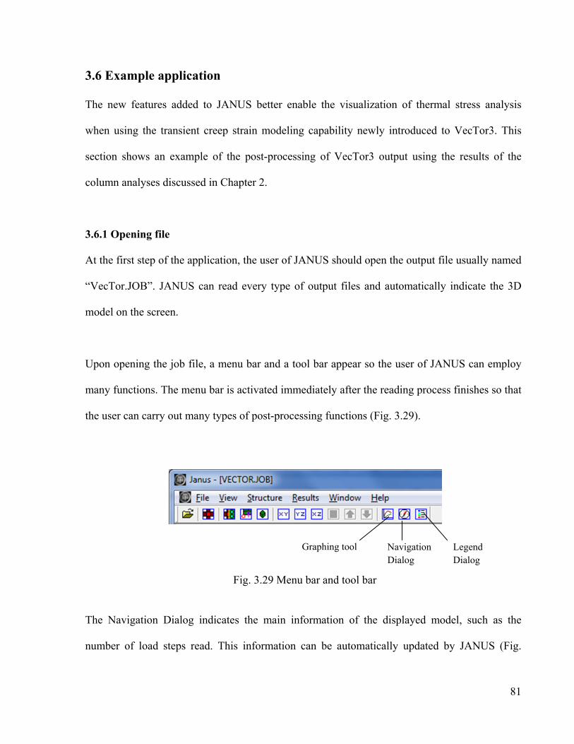
81

3.6 Example application

The new features added to JANUS better enable the visualization of thermal stress analysis

when using the transient creep strain modeling capability newly introduced to VecTor3. This

section shows an example of the post-processing of VecTor3 output using the results of the

column analyses discussed in Chapter 2.

3.6.1 Opening file

At the first step of the application, the user of JANUS should open the output file usually named

“VecTor.JOB”. JANUS can read every type of output files and automatically indicate the 3D

model on the screen.

Upon opening the job file, a menu bar and a tool bar appear so the user of JANUS can employ

many functions. The menu bar is activated immediately after the reading process finishes so that

the user can carry out many types of post-processing functions (Fig. 3.29).

The Navigation Dialog indicates the main information of the displayed model, such as the

number of load steps read. This information can be automatically updated by JANUS (Fig.

Graphing tool Navigation Dialog

Legend Dialog

Fig. 3.29 Menu bar and tool bar

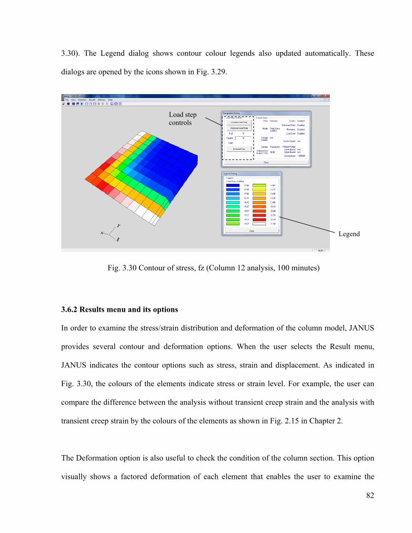
82

3.30). The Legend dialog shows contour colour legends also updated automatically. These

dialogs are opened by the icons shown in Fig. 3.29.

3.6.2 Results menu and its options

In order to examine the stress/strain distribution and deformation of the column model, JANUS

provides several contour and deformation options. When the user selects the Result menu,

JANUS indicates the contour options such as stress, strain and displacement. As indicated in

Fig. 3.30, the colours of the elements indicate stress or strain level. For example, the user can

compare the difference between the analysis without transient creep strain and the analysis with

transient creep strain by the colours of the elements as shown in Fig. 2.15 in Chapter 2.

The Deformation option is also useful to check the condition of the column section. This option

visually shows a factored deformation of each element that enables the user to examine the

Legend

Load step controls

Fig. 3.30 Contour of stress, fz (Column 12 analysis, 100 minutes)

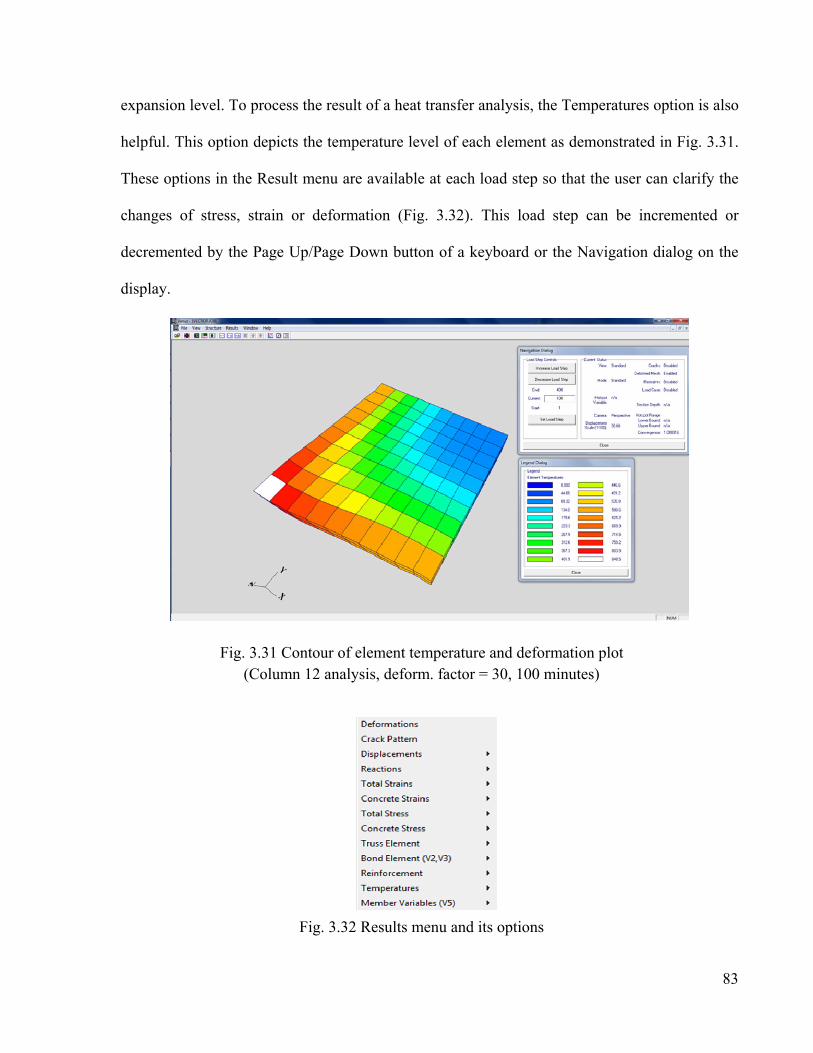
83

expansion level. To process the result of a heat transfer analysis, the Temperatures option is also

helpful. This option depicts the temperature level of each element as demonstrated in Fig. 3.31.

These options in the Result menu are available at each load step so that the user can clarify the

changes of stress, strain or deformation (Fig. 3.32). This load step can be incremented or

decremented by the Page Up/Page Down button of a keyboard or the Navigation dialog on the

display.

Fig. 3.32 Results menu and its options

Fig. 3.31 Contour of element temperature and deformation plot (Column 12 analysis, deform. factor = 30, 100 minutes)

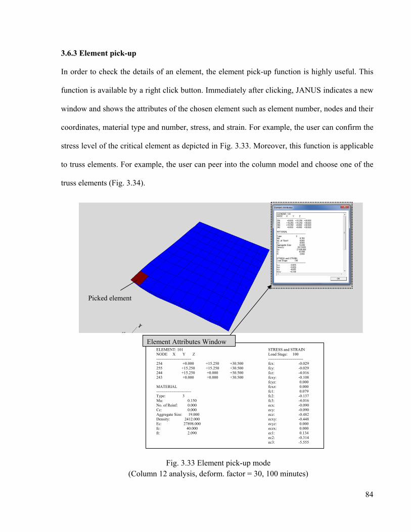
84

3.6.3 Element pick-up

In order to check the details of an element, the element pick-up function is highly useful. This

function is available by a right click button. Immediately after clicking, JANUS indicates a new

window and shows the attributes of the chosen element such as element number, nodes and their

coordinates, material type and number, stress, and strain. For example, the user can confirm the

stress level of the critical element as depicted in Fig. 3.33. Moreover, this function is applicable

to truss elements. For example, the user can peer into the column model and choose one of the

truss elements (Fig. 3.34).

Picked element

ELEMENT: 101 NODE X Y Z -------------------------- 254 +0.000 +15.250 +30.500 255 +15.250 +15.250 +30.500 244 +15.250 +0.000 +30.500 243 +0.000 +0.000 +30.500 MATERIAL -------------------------- Type: 3 Mu: 0.150 No. of Reinf: 0.000 Cc: 0.000 Aggregate Size: 19.000 Density: 2412.000 Ec: 27898.000 fc: 40.000 ft: 2.090

STRESS and STRAIN Load Stage: 100 -------------------------- fcx: -0.029 fcy: -0.029 fcz: -4.016 fcxy: -0.108 fcyz: 0.000 fcxz: 0.000 fc1: 0.079 fc2: -0.137 fc3: -4.016 ecx: -0.090 ecy: -0.090 ecz: -0.482 ecxy: -0.448 ecyz: 0.000 eczx: 0.000 ec1: 0.134 ec2: -0.314 ec3: -5.555

Element Attributes Window

Fig. 3.33 Element pick-up mode (Column 12 analysis, deform. factor = 30, 100 minutes)

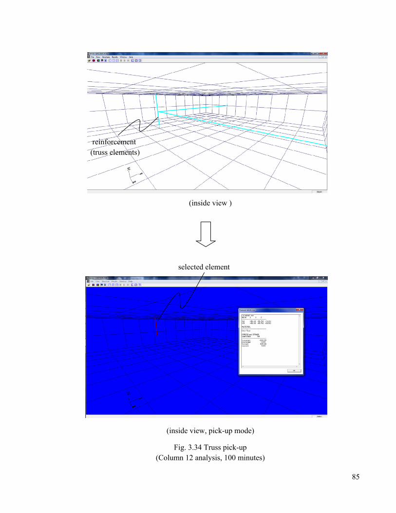
85

Fig. 3.34 Truss pick-up (Column 12 analysis, 100 minutes)

(inside view )

reinforcement (truss elements)

(inside view, pick-up mode)

selected element

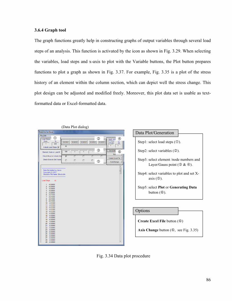
86

3.6.4 Graph tool

The graph functions greatly help in constructing graphs of output variables through several load

steps of an analysis. This function is activated by the icon as shown in Fig. 3.29. When selecting

the variables, load steps and x-axis to plot with the Variable buttons, the Plot button prepares

functions to plot a graph as shown in Fig. 3.37. For example, Fig. 3.35 is a plot of the stress

history of an element within the column section, which can depict well the stress change. This

plot design can be adjusted and modified freely. Moreover, this plot data set is usable as text-

formatted data or Excel-formatted data.

Fig. 3.34 Data plot procedure

(Data Plot dialog)

Step1: select load steps ().

Step2: select variables ().

Step3: select element /node numbers and Layer/Gauss point ( & ).

Step4: select variables to plot and set X-axis ().

Step5: select Plot or Generating Data button ().

Data Plot/Generation

Create Excel File button ()

Axis Change button (, see Fig. 3.35)

Options

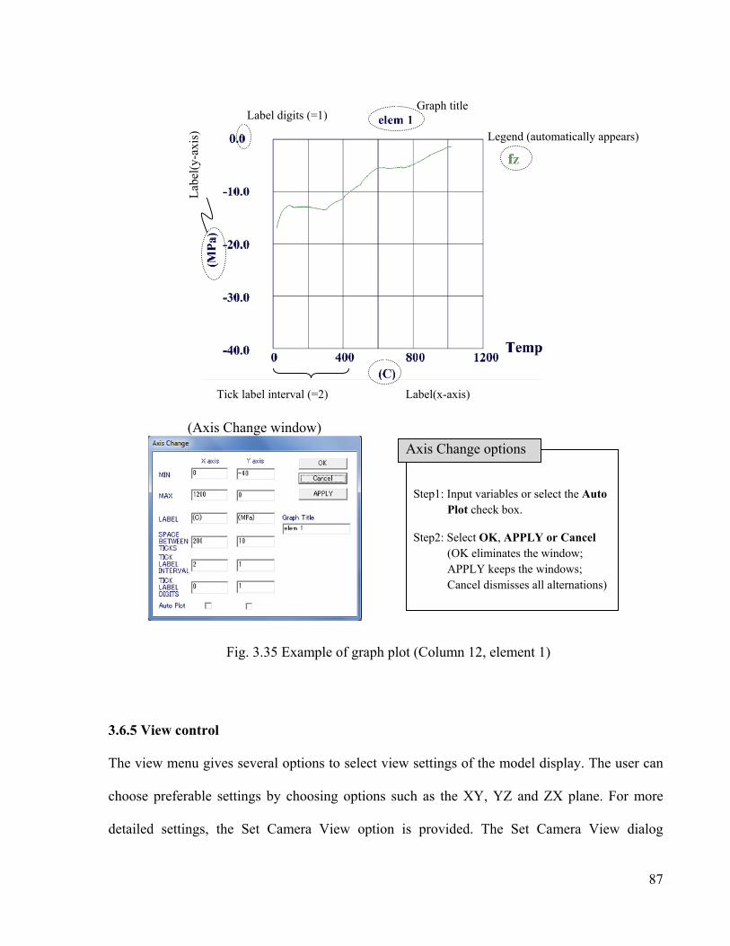
87

3.6.5 View control

The view menu gives several options to select view settings of the model display. The user can

choose preferable settings by choosing options such as the XY, YZ and ZX plane. For more

detailed settings, the Set Camera View option is provided. The Set Camera View dialog

(Axis Change window)

Lab

el(y

-axi

s)

Step1: Input variables or select the Auto Plot check box.

Step2: Select OK, APPLY or Cancel (OK eliminates the window;

APPLY keeps the windows; Cancel dismisses all alternations)

Axis Change options

Label(x-axis) Tick label interval (=2)

Label digits (=1) Graph title

Legend (automatically appears)

Fig. 3.35 Example of graph plot (Column 12, element 1)

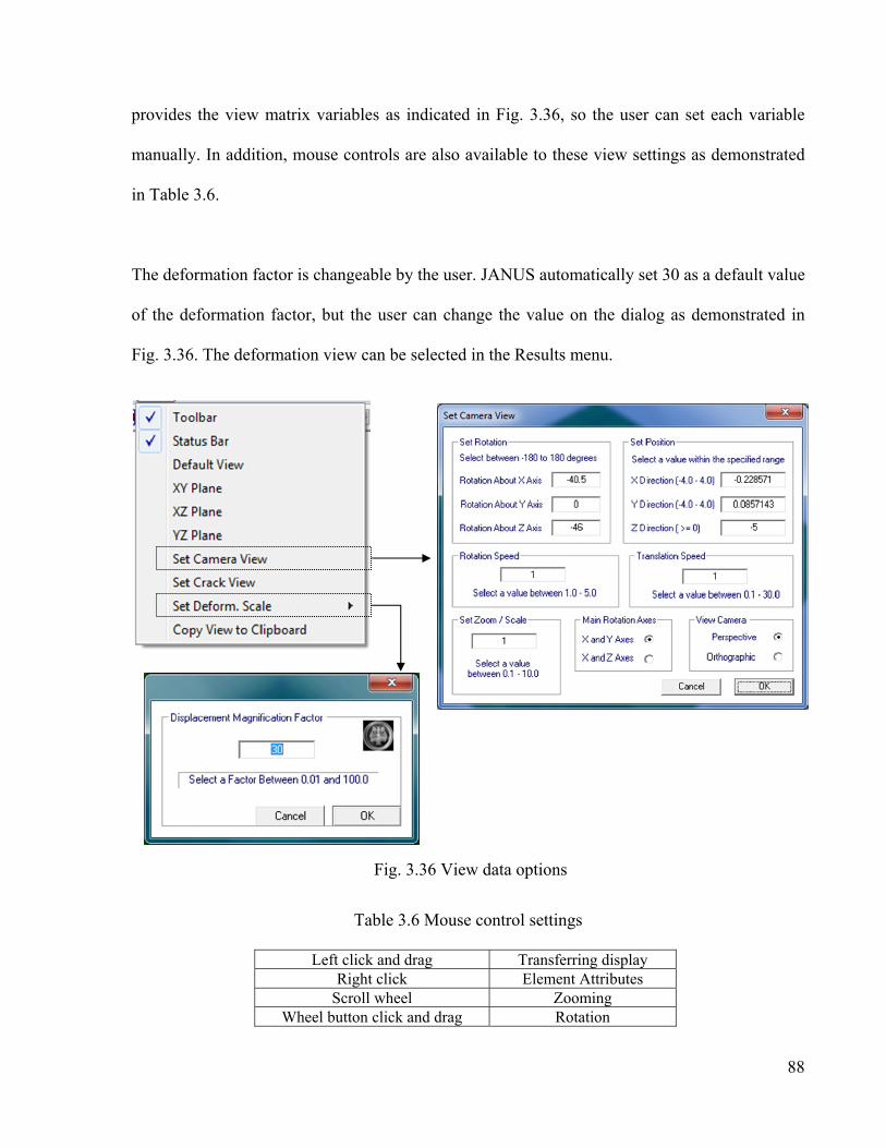
88

provides the view matrix variables as indicated in Fig. 3.36, so the user can set each variable

manually. In addition, mouse controls are also available to these view settings as demonstrated

in Table 3.6.

The deformation factor is changeable by the user. JANUS automatically set 30 as a default value

of the deformation factor, but the user can change the value on the dialog as demonstrated in

Fig. 3.36. The deformation view can be selected in the Results menu.

Table 3.6 Mouse control settings

Left click and drag Transferring display Right click Element Attributes

Scroll wheel Zooming Wheel button click and drag Rotation

Fig. 3.36 View data options

89

CHAPTER 4: Conclusions

A suite of NLFEA programs, VecTor, has been developed at the University of Toronto.

However, this software still requires the development of other functions to execute some types

of analysis. One of the required functions is the consideration of transient creep strain in

structures involving heat transfer analysis. Moreover, there has been a long-standing need to

develop a general graphics-based post-processor for VecTor.

The first objective of this thesis was to develop and implement a model considering the effect of

the transient creep strain; this mechanism can have significant influence on the behaviour of

concrete under elevated temperatures. VecTor3 can now analyze the behaviour of the concrete

including the effect of the transient creep strain. Moreover, this thesis confirmed that the new

function worked properly and showed how transient creep strain alters the analysis result.

Although more studies are needed to conclude its influence on the behaviour of concrete under

high temperatures, preliminary analysis results suggest that new insights can be achieved with

investigations using this program.

The second objective of this thesis was to construct new analysis visualization features

compatible with entire suite of VecTor programs. The modified post-processor, JANUS, has had

its abilities expanded. Powerful features added include the following:

・ accommodation of all structure types (VecTor2 to VecTor6),

・ new ability to process temperature output,

・ graphing and data generating functions,

90

・ element pick-up functions invoked by a simple and intuitive operation, and

・ accommodation of free format job files.

Considering the memory size and the development environment of JANUS as mentioned in the

section 3.3, recommendations are as follows:

・ the adoption of a unified format for all VecTor files, and

・ a unified description of variables in the output files.

91

References

Anderburg, Y., and Thelandersson, S. (1976). Stress and Deformation Characteristics of Concrete at High Temperatures. Lund: Lund Institute of Technology, Division of Structural Mechanics and Concrete Construction.

Arthananari, S., and Yu, C. W. (1967). Creep of Concrete Under Uniaxial and Biaxial Stresses at Elevated Temperatures. Magazine of Concrete Research, 19(60), 149-156.

ASTM. (1979). Standard Methods of Fire Tests of Building Construction and Materials. Philadelphia: American Society for Testing and Materials.

CEN. (1995). ENV 1992-1-2:1995 Eurocode 2: Design of Concrete Structures, Part 1-2: General Rules-Structural Fire Design. Brussels: CEN ENV, Commission of European Communities.

CEN. (2004). ENV 1992-1-2:2004 Eurocode 2: Design of Concrete Structures, Part 1-2: General Rules-Structural Fire Design. Brussels: CEN ENV, Commission of European Communities.

CEN. (2005). ENV 1994-1-2:2005 Eurocode 4: Design of Composite Steel and Concrete Structures, Part 1-2: General Rules-Structural Fire Design. Brussels: CEN ENV, Commission of European Communities.

Cruz, C. R. (1968). Apparatus for Measuring Creep of Concrete at Elevated Temperature. Journal of PCA Research and Development Laboratories, PCA Research and Development Bulletin 225, 10(3), 36-42.

Gernay, T. (2012). Effect of Transient Creep Strain Model on the Behavior of Concrete Columns Subjected to Heating and Cooling. Fire Technology, 313-329.

Gvozdev, A. A. (1966). Creep of Concrete. Mekhanika Tverdogo Tela, 137-152.

Khory, G. A., Pesavento, F., and Schrefler, B. A. (2002). Modelling of heated concrete. Magazine of Concrete Research, 54(2), 77-101.

Lie, T. T., and Lin, T. D. (1983a). Fire Tests on Reinforced Concrete Columns, Specimen No. 10. Division of Building Research. Ottawa: National Research Counsil of Canada.

Lie, T. T., and Lin, T. D. (1983b). Fire Tests on Reinforced Concrete Columns, Specimen No. 11. Division of Building Research. Ottawa: National Research Counsil of Canada.

Lie, T. T., and Lin, T. D. (1983c). Fire Tests on Reinforced Concrete Columns, Specimen No. 12. Division of Building Research. Ottawa: National Research Counsil of Canada.

92

Marechal, J. C. (1972). Creep of Concrete as a Function of Temperature. International Seminar on Concrete for Nuclear Reactors (pp. 547-564). Berlin: American Concrete Institute.

Miura, I., Itatani, T., and Hakamaya, H. (2007). Study on Determination Method with Color of Test-paper of - Decision Method with Construction Time of Coating Floor-. Toda Corp. Technical Report, 33, 11.

MSDN. (2013). MDIDOCVW Sample: Demonstrates MDI Using Doc/View Architecture. (Microsoft) Retrieved April 24, 2013, from Microsoft Developer Network: http://msdn.microsoft.com/en-us/library/cstcs513(v=vs.80).aspx

Schneider, U. (1979). Ein Beitrag zur Klärung des Kriechens und der Relaxation von Beton unterinstationärer Temperatureinwirkung (Creep and Relaxation of Concrete Under Transient Temperature Conditions). Forschungsbeiträge für die Baupraxis, 133-149.

Vecchio, F. J., and Collins, M. P. (1986). The Modified Compression Field Theory for Reinforced Concrete Elements Subjected to Shear. ACI Journal, 83(2), 219-231.

Vecchio, F. J., Bentz, E. C., and Collins, M. P. (2004). Tools for forensic analysis of concrete structures. Computers and Concrete, 1(1), 1-14.

Yamamoto, N. (1999). Visual C++ vol.1 Intermediate Windows Programming (Learning Programming Series). Tokyo, Japan: Shoueisha.