Normal Distribution

Continuous Random VariablesContinuous Random Variables• Continuous random variables can assume

the infinitely many values corresponding to points on a line interval.

• Examples:Examples:

– Heights, weights

– length of life of a particular product

– experimental laboratory error

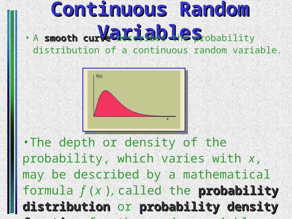
Continuous Random VariablesContinuous Random Variables• A smooth curvesmooth curve describes the probability

distribution of a continuous random variable.

•The depth or density of the probability, which varies with x, may be described by a mathematical formula f (x ), called the probability distributionprobability distribution or probability density functionprobability density function for the random variable x.

Properties of ContinuousProperties of ContinuousProbability DistributionsProbability Distributions

• The area under the curve is equal to 1.1.• P(a x b) = area under the curvearea under the curve

between a and b.

•There is no probability attached to any single value of x. That is, P(x = a) = 0.

Continuous Probability Continuous Probability DistributionsDistributions

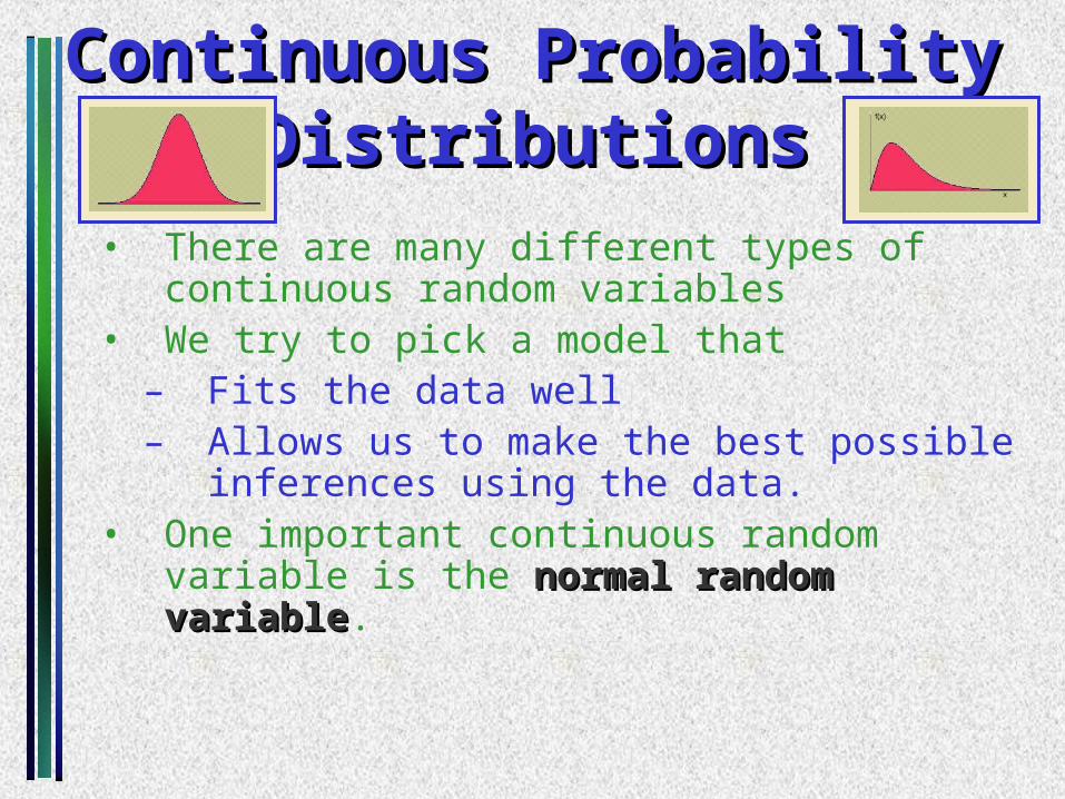
• There are many different types of continuous random variables

• We try to pick a model that– Fits the data well– Allows us to make the best possible

inferences using the data.• One important continuous random variable is

the normal random variablenormal random variable.

The Standard Normal The Standard Normal DistributionDistribution

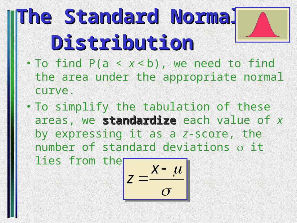
• To find P(a < x < b), we need to find the area under the appropriate normal curve.

• To simplify the tabulation of these areas, we standardize standardize each value of x by expressing it as a z-score, the number of standard deviations it lies from the mean .

x

z

x

z

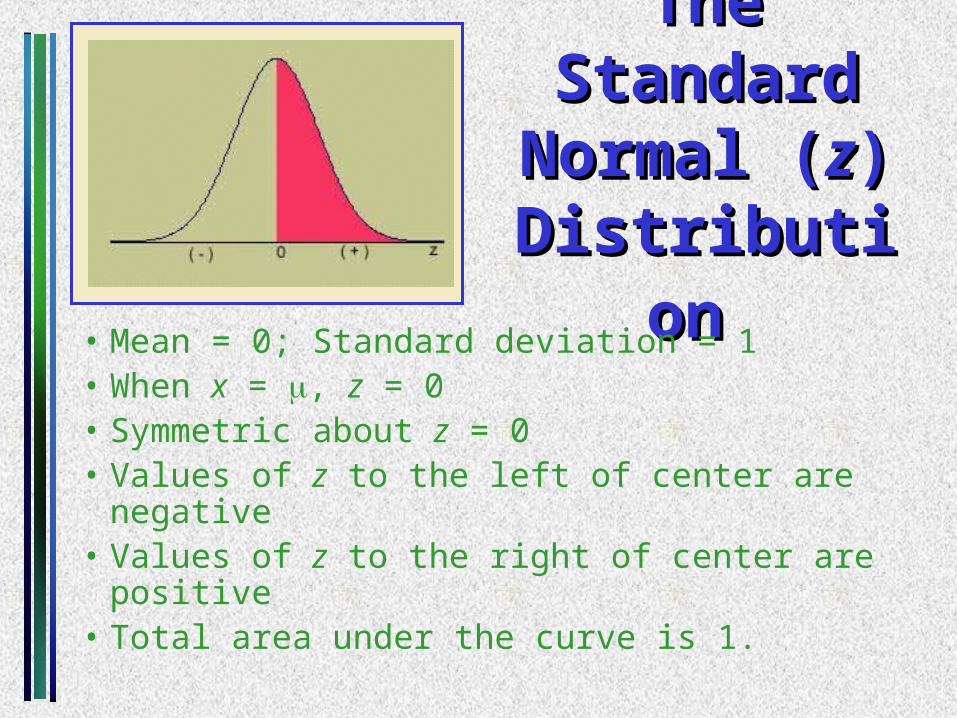
The Standard The Standard Normal (Normal (zz) )

DistributionDistribution • Mean = 0; Standard deviation = 1• When x = , z = 0• Symmetric about z = 0• Values of z to the left of center are negative• Values of z to the right of center are positive• Total area under the curve is 1.

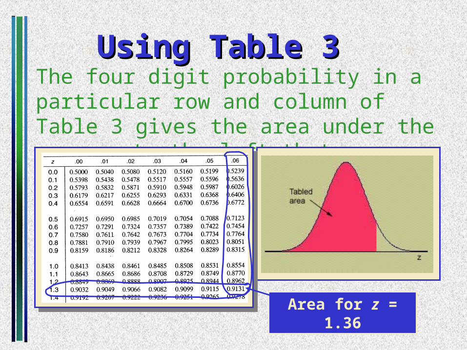
Using Table 3Using Table 3The four digit probability in a particular row and column of Table 3 gives the area under the z curve to the left that particular value of z.

Area for z = 1.36

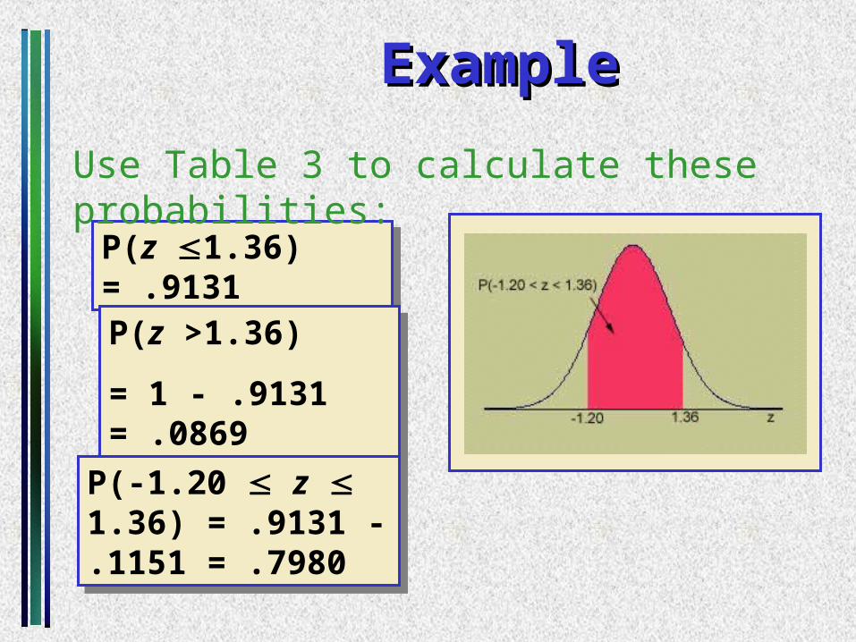
P(z 1.36) = .9131P(z 1.36) = .9131

P(z >1.36)

= 1 - .9131 = .0869

P(z >1.36)

= 1 - .9131 = .0869

P(-1.20 z 1.36) = .9131 - .1151 = .7980

P(-1.20 z 1.36) = .9131 - .1151 = .7980

ExampleExample

Use Table 3 to calculate these probabilities:

To find an area to the left of a z-value, find the area directly from the table.To find an area to the right of a z-value, find the area in Table 3 and subtract from 1.To find the area between two values of z, find the two areas in Table 3, and subtract one from the other.

To find an area to the left of a z-value, find the area directly from the table.To find an area to the right of a z-value, find the area in Table 3 and subtract from 1.To find the area between two values of z, find the two areas in Table 3, and subtract one from the other.

P(-1.96 z 1.96) = .9750 - .0250 = .9500

P(-1.96 z 1.96) = .9750 - .0250 = .9500P(-3 z 3)= .9987 - .0013=.9974

P(-3 z 3)= .9987 - .0013=.9974

Using Table 3Using Table 3

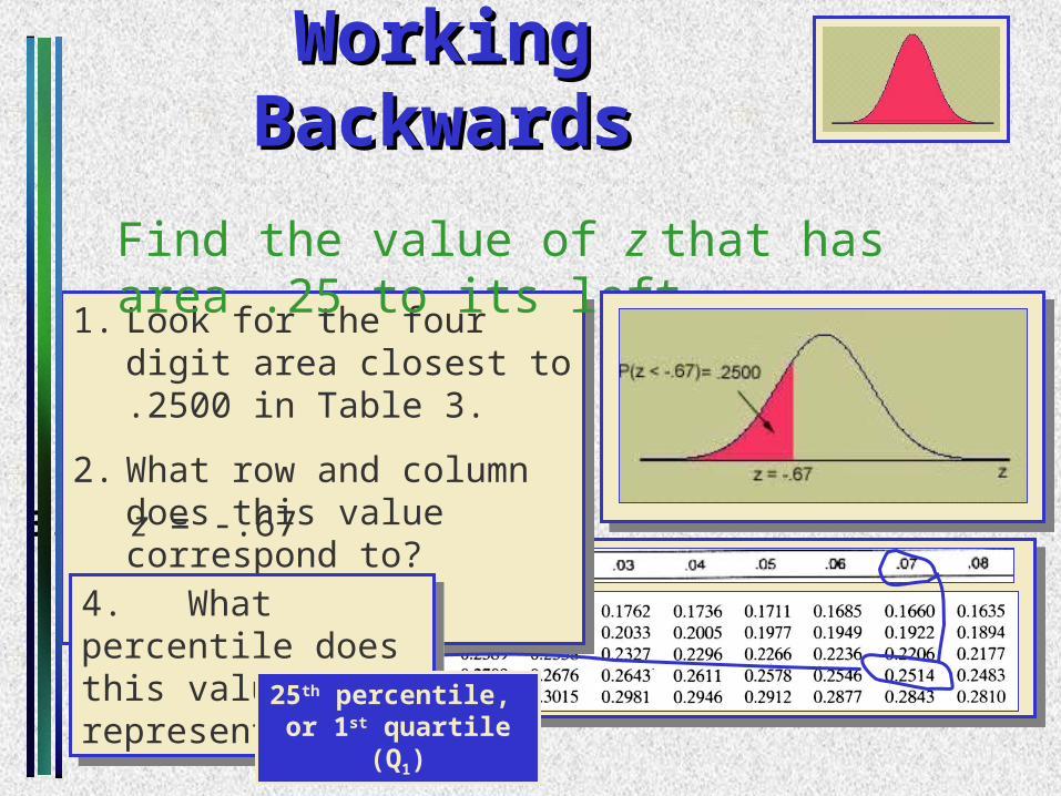
1. Look for the four digit area closest to .2500 in Table 3.

2. What row and column does this value correspond to?


2. What row and column does this value correspond to?

Working BackwardsWorking Backwards

Find the value of z that has area .25 to its left.

4. What percentile does this value represent?

4. What percentile does this value represent? 25th percentile,

or 1st quartile (Q1)

3. z = -.67

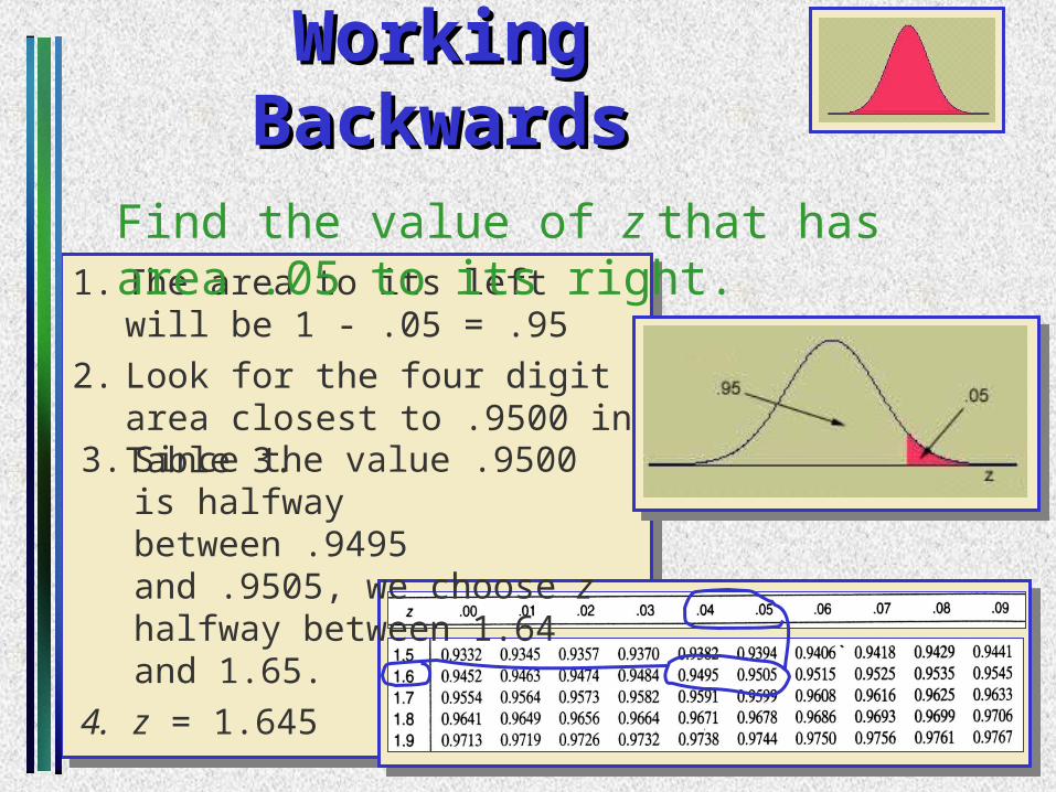
1. The area to its left will be 1 - .05 = .95


1. The area to its left will be 1 - .05 = .95


Working BackwardsWorking Backwards

Find the value of z that has area .05 to its right.

3. Since the value .9500 is halfway between .9495 and .9505, we choose z halfway between 1.64 and 1.65.

4. z = 1.645

Finding Probabilities for the Finding Probabilities for the General Normal Random VariableGeneral Normal Random Variable

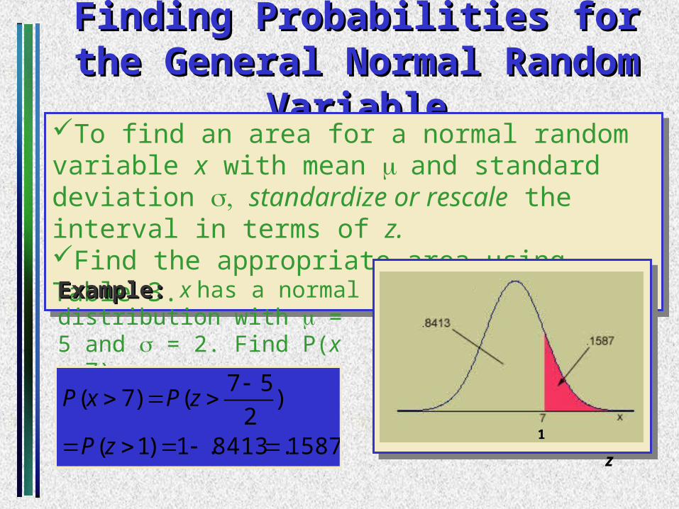
To find an area for a normal random variable x with mean and standard deviation standardize or rescale the interval in terms of z. Find the appropriate area using Table 3.

To find an area for a normal random variable x with mean and standard deviation standardize or rescale the interval in terms of z. Find the appropriate area using Table 3.

Example: Example: x has a normal distribution with = 5 and = 2. Find P(x > 7).

1587.8413.1)1(

)2

57()7(

zP

zPxP

1 z

ExampleExample

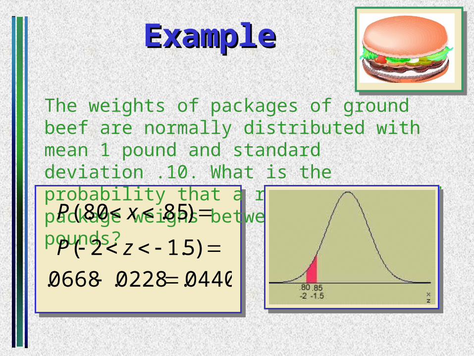
The weights of packages of ground beef are normally distributed with mean 1 pound and standard deviation .10. What is the probability that a randomly selected package weighs between 0.80 and 0.85 pounds?

)85.80(. xP

)5.12( zP

0440.0228.0668.

Key ConceptsKey ConceptsI. Continuous Probability DistributionsI. Continuous Probability Distributions

1. Continuous random variables

2. Probability distributions or probability density functions

a. Curves are smooth.

b. The area under the curve between a and b represents

the probability that x falls between a and b.

c. P (x a) 0 for continuous random variables.

II. The Normal Probability DistributionII. The Normal Probability Distribution

1. Symmetric about its mean .

2. Shape determined by its standard deviation .

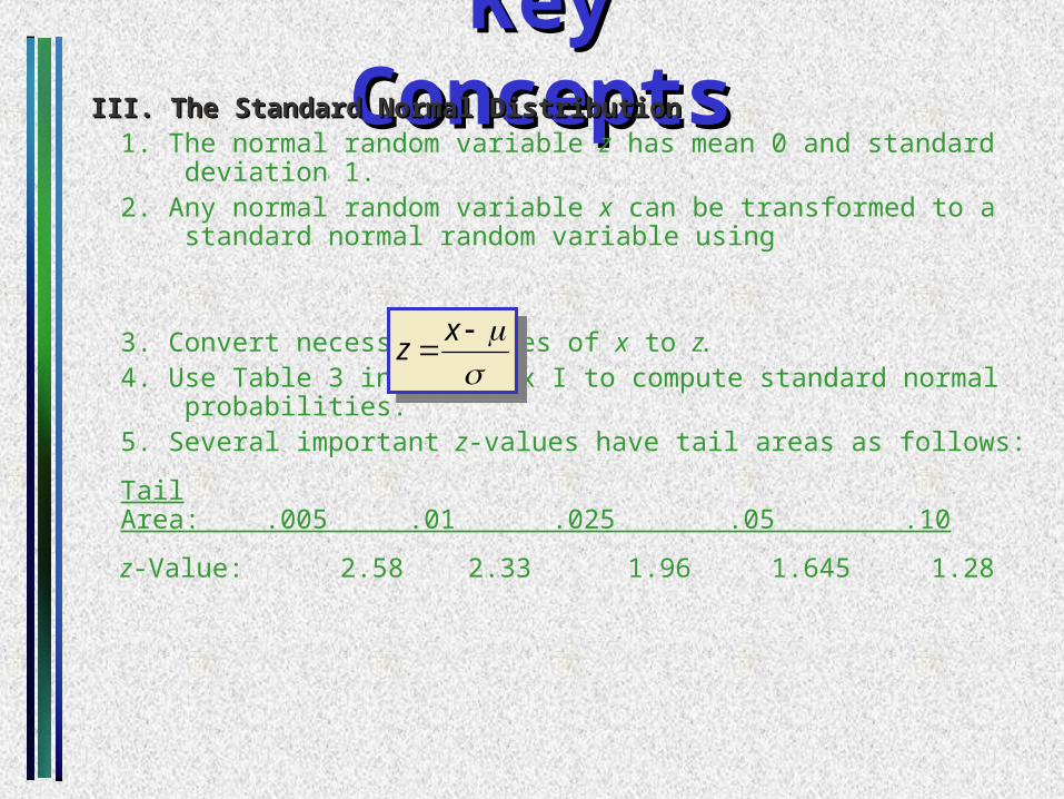
Key ConceptsKey ConceptsIII. The Standard Normal DistributionIII. The Standard Normal Distribution

1. The normal random variable z has mean 0 and standard deviation 1.2. Any normal random variable x can be transformed to a standard normal random variable using

3. Convert necessary values of x to z.4. Use Table 3 in Appendix I to compute standard normal probabilities.5. Several important z-values have tail areas as follows:

Tail Area: .005 .01 .025 .05 .10

z-Value: 2.58 2.33 1.96 1.645 1.28

x

z

x

z

Documents

Normal Distribution