Normal Distributions (2)

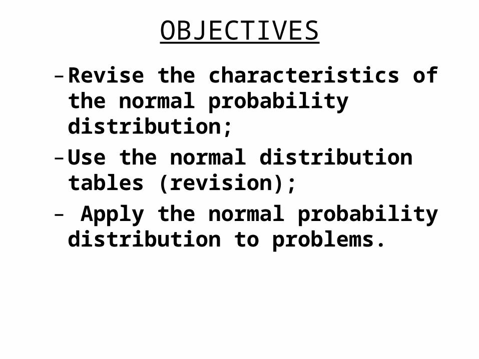
OBJECTIVES

– Revise the characteristics of the normal probability distribution;

– Use the normal distribution tables (revision);

– Apply the normal probability distribution to problems.

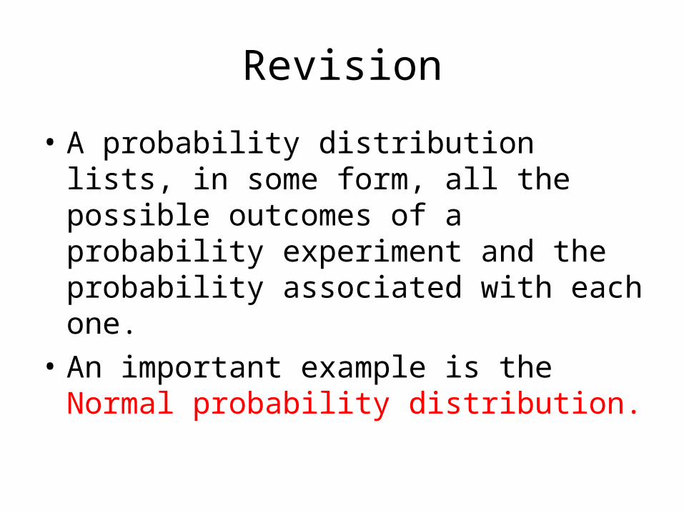
Revision

• A probability distribution lists, in some form, all the possible outcomes of a probability experiment and the probability associated with each one.

• An important example is the Normal probability distribution.

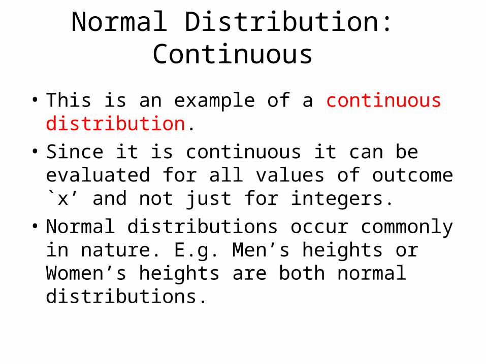
Normal Distribution: Continuous

• This is an example of a continuous distribution.

• Since it is continuous it can be evaluated for all values of outcome `x’ and not just for integers.

• Normal distributions occur commonly in nature. E.g. Men’s heights or Women’s heights are both normal distributions.

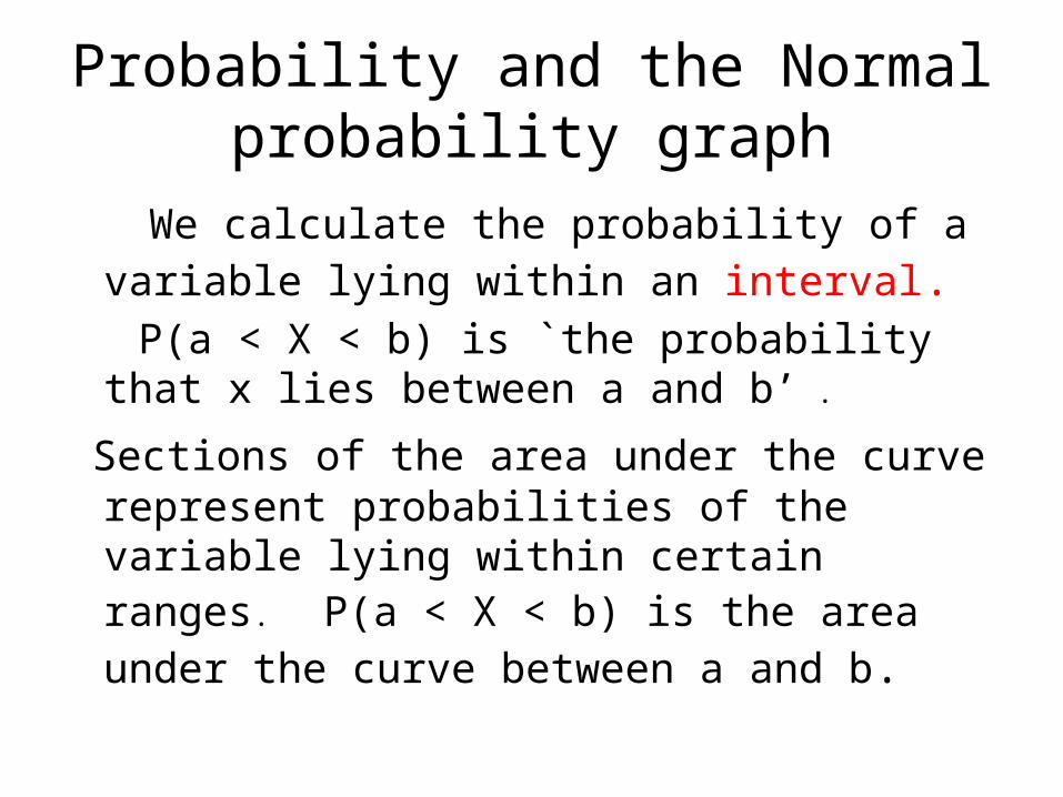
Probability and the Normal probability graph

We calculate the probability of a variable lying within an interval.

P(a < X < b) is `the probability that x lies between a and b’ .

Sections of the area under the curve represent probabilities of the variable lying within certain ranges. P(a < X < b) is the area under the curve between a and b.

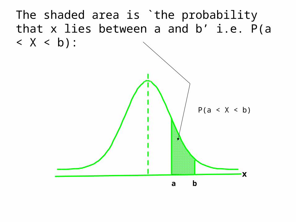
The shaded area is `the probability that x lies between a and b’ i.e. P(a < X < b):

a bx

P(a < X < b)

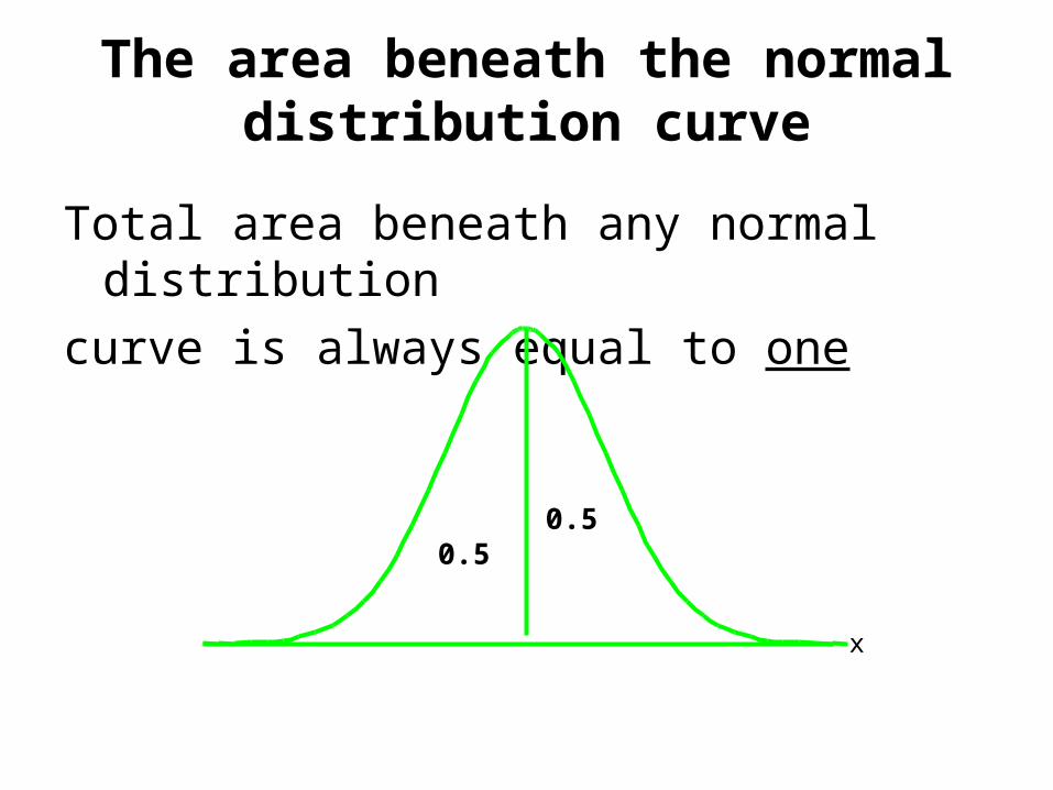
The area beneath the normal distribution curve

Total area beneath any normal distribution

curve is always equal to one

0.5

0.5

x

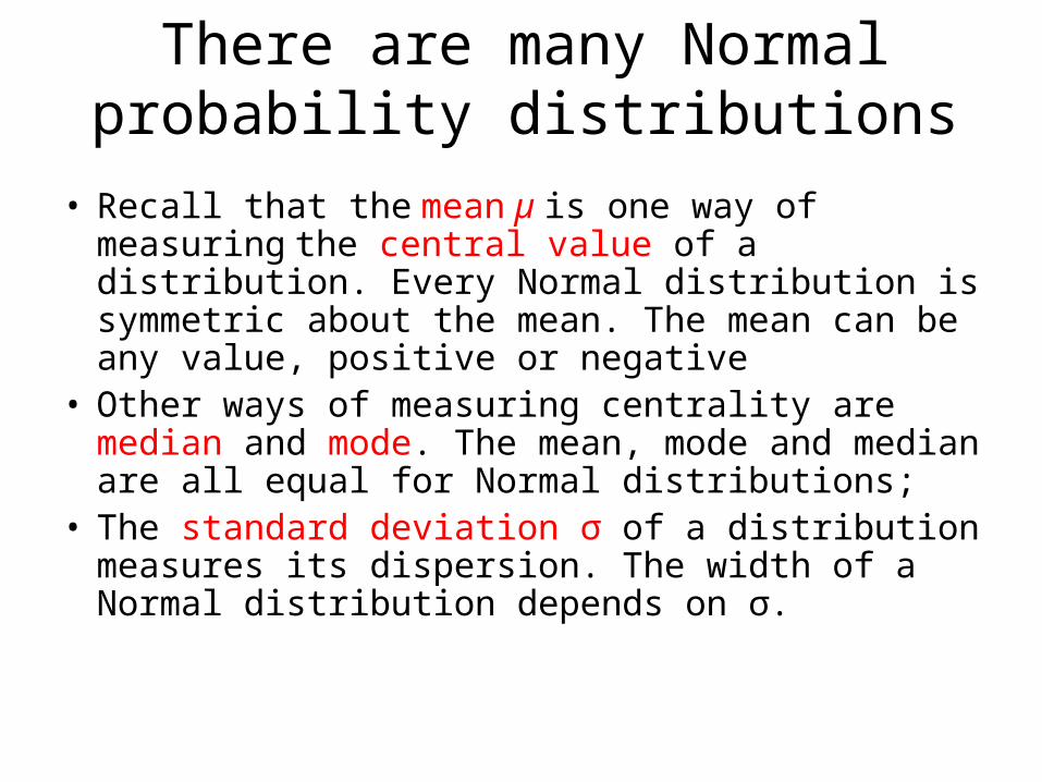
There are many Normal probability distributions

• Recall that the mean µ is one way of measuring the central value of a distribution. Every Normal distribution is symmetric about the mean. The mean can be any value, positive or negative

• Other ways of measuring centrality are median and mode. The mean, mode and median are all equal for Normal distributions;

• The standard deviation σ of a distribution measures its dispersion. The width of a Normal distribution depends on σ.

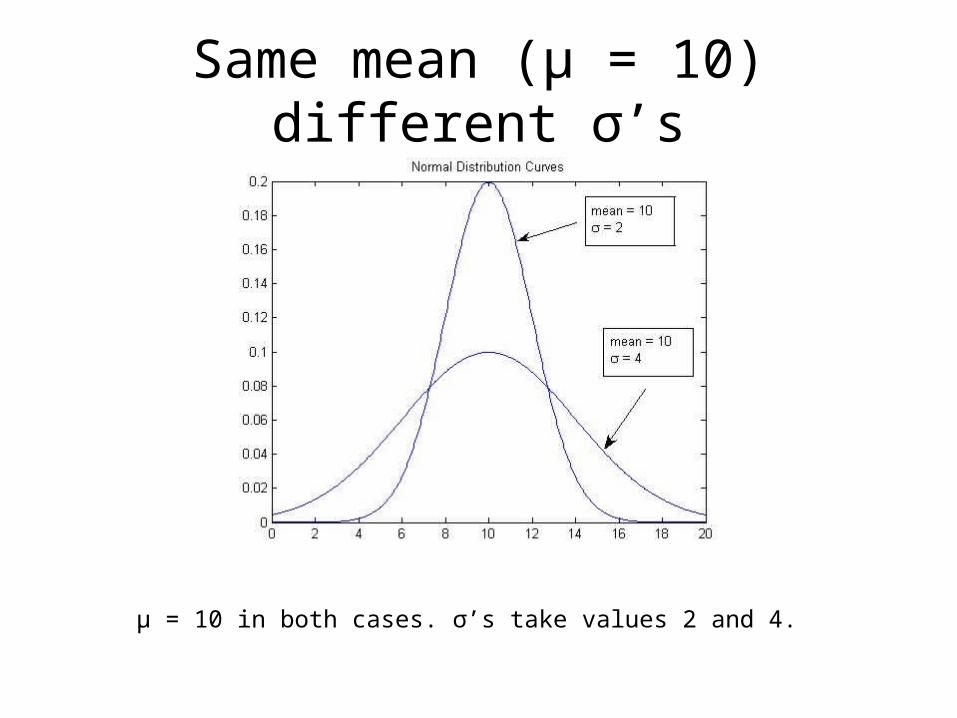
Same mean (µ = 10) different σ’s

µ = 10 in both cases. σ’s take values 2 and 4.

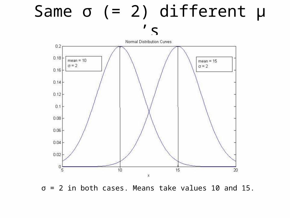
Same σ (= 2) different µ ’s

σ = 2 in both cases. Means take values 10 and 15.

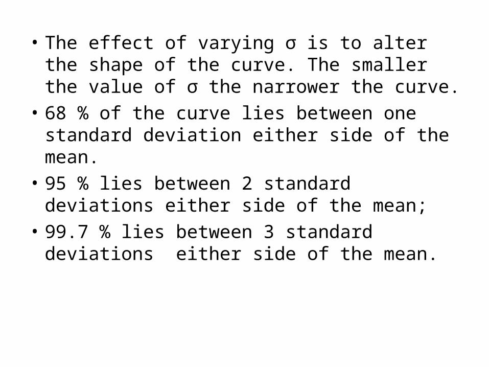
• The effect of varying σ is to alter the shape of the curve. The smaller the value of σ the narrower the curve.

• 68 % of the curve lies between one standard deviation either side of the mean.

• 95 % lies between 2 standard deviations either side of the mean;

• 99.7 % lies between 3 standard deviations either side of the mean.

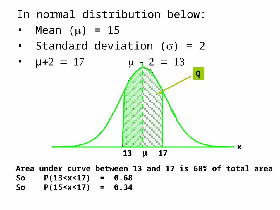
In normal distribution below:• Mean () = 15• Standard deviation () = 2• µ

13 17

Area under curve between 13 and 17 is 68% of total areaSo P(13<x<17) = 0.68So P(15<x<17) = 0.34

Q

x

Standardising

• The x value will not always be an exact number of standard deviations away from the mean.

• We can calculate the number of standard deviations which x lies away from the mean.

• Standardised value (z) can be obtained from tables. (See handout.)

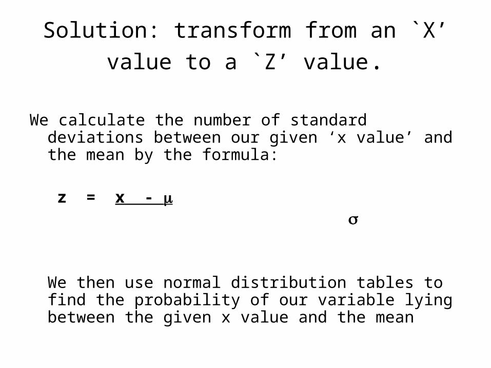
Solution: transform from an `X’ value to a `Z’

value.

We calculate the number of standard deviations between our given ‘x value’ and the mean by the formula:

z = x -

We then use normal distribution tables to find the probability of our variable lying between the given x value and the mean

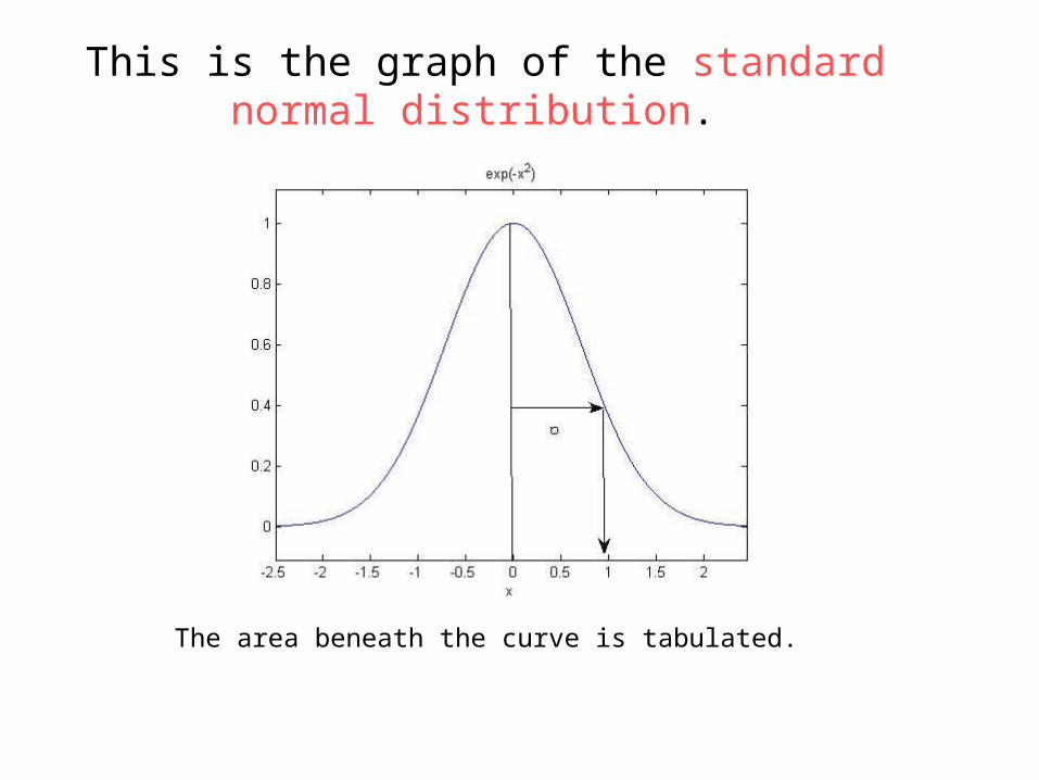
This is the graph of the standard normal distribution.

The area beneath the curve is tabulated.

The standard Normal distribution

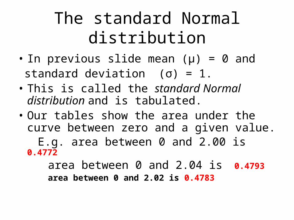
• In previous slide mean (µ) = 0 and standard deviation (σ) = 1.• This is called the standard Normal

distribution and is tabulated.• Our tables show the area under the curve

between zero and a given value. E.g. area between 0 and 2.00 is 0.4772

area between 0 and 2.04 is 0.4793

area between 0 and 2.02 is 0.4783

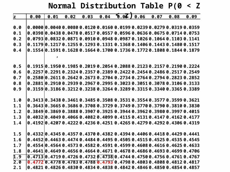
z 0.00 0.01 0.02 0.03 0.04 0.05 0.06 0.07 0.08 0.09

0.0 0.0000 0.0040 0.0080 0.0120 0.0160 0.0199 0.0239 0.0279 0.0319 0.03590.1 0.0398 0.0438 0.0478 0.0517 0.0557 0.0596 0.0636 0.0675 0.0714 0.07530.2 0.0793 0.0832 0.0871 0.0910 0.0948 0.0987 0.1026 0.1064 0.1103 0.11410.3 0.1179 0.1217 0.1255 0.1293 0.1331 0.1368 0.1406 0.1443 0.1480 0.15170.4 0.1554 0.1591, 0.1628 0.1664 0.1700 0.1736 0.1772 0.1808 0.1844 0.1879

0.5 0.1915 0.1950 0.1985 0.2019 0.2054 0.2088 0.2123 0.2157 0.2190 0.22240.6 0.2257 0.2291 0.2324 0.2357 0.2389 0.2422 0.2454 0.2486 0.2517 0.25490.7 0.2580 0.2611 0.2642 0.2673 0.2704 0.2734 0.2764 0.2794 0.2823 0.28520.8 0.2881 0.2910 0.2939 0.2967 0.2995 0.3023 0.3051 0.3078 0.3106 0.31330.9 0.3159 0.3186 0.3212 0.3238 0.3264 0.3289 0.3315 0.3340 0.3365 0.3389

1.0 0.3413 0.3438 0.3461 0.3485 0.3508 0.3531 0.3554 0.3577 0.3599 0.36211.1 0.3643 0.3665 0.3686 0.3708 0.3729 0.3749 0.3770 0.3790 0.3810 0.38301.2 0.3849 0.3869 0.3888 0.3907 0.3925 0.3944 0.3962 0.3980 0.3997 0.40151.3 0.4032 0.4049 0.4066 0.4082 0.4099 0.4115 0.4131 0.4147 0.4162 0.41771.4 0.4192 0.4207 0.4222 0.4236 0.4251 0.4265 0.4279 0.4292 0.4306 0.4319

1.5 0.4332 0.4345 0.4357 0.4370 0.4382 0.4394 0.4406 0.4418 0.4429 0.44411.6 0.4452 0.4463 0.4474 0.4484 0.4495 0.4505 0.4515 0.4525 0.4535 0.45451.7 0.4554 0.4564 0.4573 0.4582 0.4591 0.4599 0.4608 0.4616 0.4625 0.46331.8 0.4641 0.4649 0.4656 0.4664 0.4671 0.4678 0.4686 0.4693 0.4699 0.47061.92.02.1

0.47130.47720.4821

0.47190.47780.4826

0.47260.47830.4830

0.47320.47880.4834

0.47380.47930.4838

0.47440.47980.4842

0.47500.48030.4846

0.47560.48080.4850

0.47610.48120.4854

0.47670.48170.4857

Normal Distribution Table P(0 < Z < z)

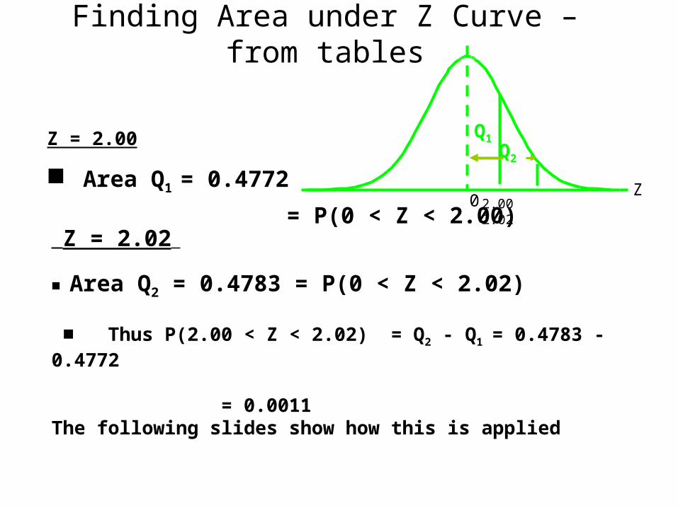
Finding Area under Z Curve – from tables

Z = 2.00

■ Area Q1 = 0.4772

= P(0 < Z < 2.00)

Q1

0 2.00 2.02

Z = 2.02

■ Area Q2 = 0.4783 = P(0 < Z < 2.02)

■ Thus P(2.00 < Z < 2.02) = Q2 - Q1 = 0.4783 - 0.4772 = 0.0011The following slides show how this is applied

Z

Q2

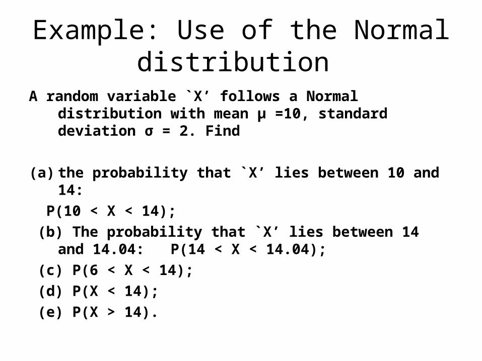
Example: Use of the Normal distribution

A random variable `X’ follows a Normal distribution with mean µ =10, standard deviation σ = 2. Find

(a) the probability that `X’ lies between 10 and 14:

P(10 < X < 14);

(b) The probability that `X’ lies between 14 and 14.04: P(14 < X < 14.04);

(c) P(6 < X < 14);

(d) P(X < 14);

(e) P(X > 14).

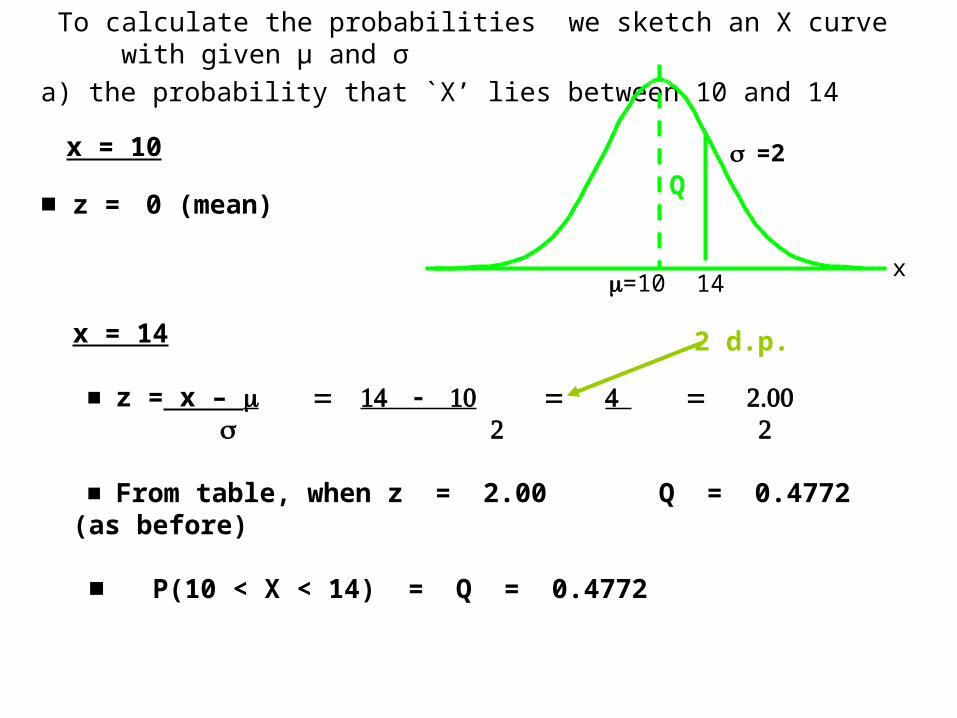
a) the probability that `X’ lies between 10 and 14

x = 10

■ z = 0 (mean)

To calculate the probabilities we sketch an X curve with given µ and σ

Q

=10

14

=2

x = 14

■ z = x –

■ From table, when z = 2.00 Q = 0.4772 (as before)

■ P(10 < X < 14) = Q = 0.4772

x

2 d.p.

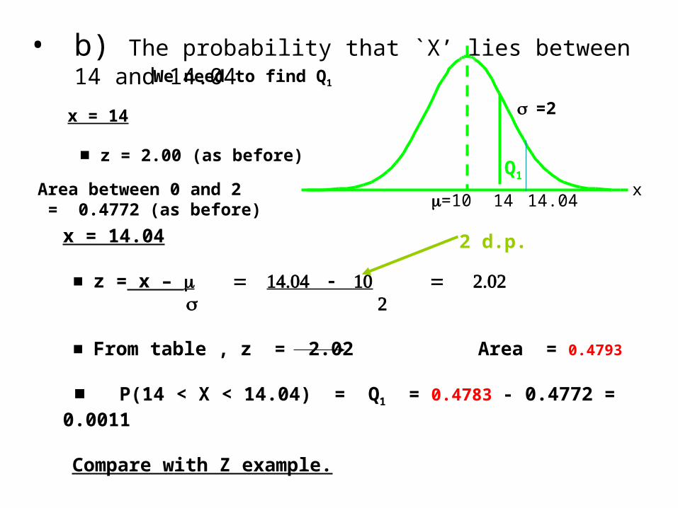
• b) The probability that `X’ lies between 14 and 14.04

Q1

=10

14

=2

x = 14.04

■ z = x –

■ From table , z = 2.02 Area = 0.4793

■ P(14 < X < 14.04) = Q1 = 0.4783 - 0.4772 = 0.0011

Compare with Z example.

x

2 d.p.

14.04

x = 14

■ z = 2.00 (as before)

Area between 0 and 2 = 0.4772 (as before)

We need to find Q1

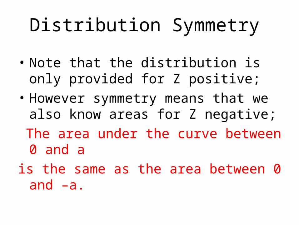
Distribution Symmetry

• Note that the distribution is only provided for Z positive;

• However symmetry means that we also know areas for Z negative;

The area under the curve between 0 and a

is the same as the area between 0 and –a.

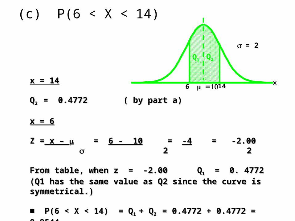
(c) P(6 < X < 14)

14

= 2

Q1 Q2

6x = 14x = 14

QQ2 2 = 0.4772 = 0.4772 ( by part a) ( by part a)

x = 6x = 6

Z =Z = x – x – = = 6 - 106 - 10 = = -4-4 = -2.00 = -2.00 2 22 2

From table, when z = -2.00 QFrom table, when z = -2.00 Q11 = 0. = 0. 4772 4772

(Q1 has the same value as Q2 since the curve is symmetrical.)(Q1 has the same value as Q2 since the curve is symmetrical.)

■ ■ P(6 < X < 14) = QP(6 < X < 14) = Q1 1 + Q+ Q2 2 = 0.4772 + 0.4772 = = 0.4772 + 0.4772 = 0.95440.9544

x

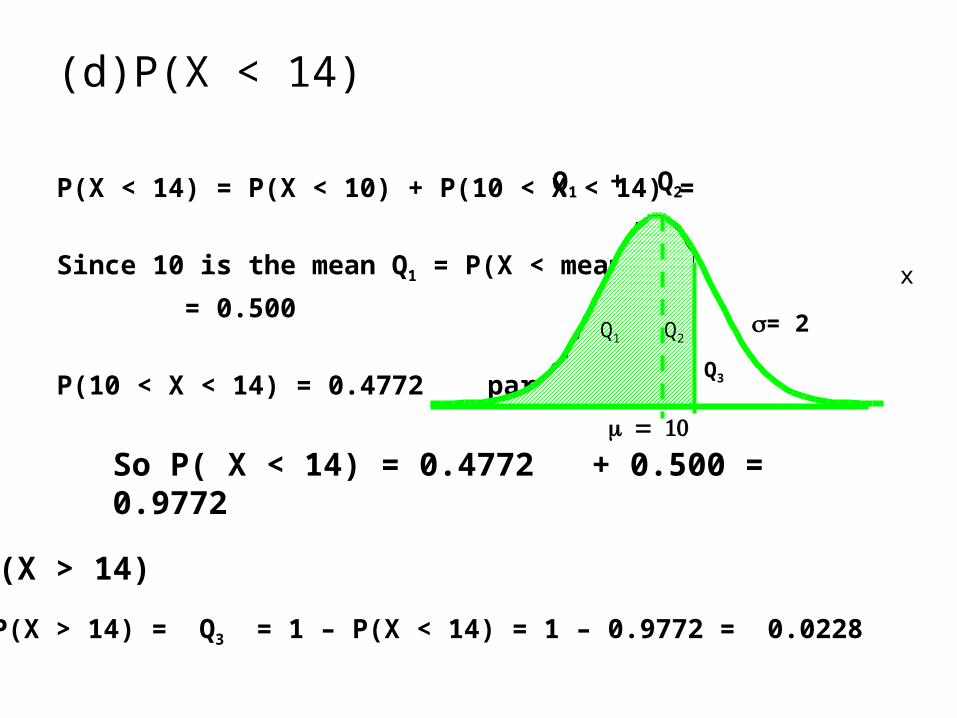
(d) P(X < 14)

P(X < 14) = P(X < 10) + P(10 < X < 14) =

Since 10 is the mean Q1 = P(X < mean)

= 0.500

P(10 < X < 14) = 0.4772 part (a)

= 2

x

Q2

Q1 + Q2

Q1

So P( X < 14) = 0.4772 + 0.500 = 0.9772

Q3

(e) P(X > 14)

P(X > 14) = Q3 = 1 – P(X < 14) = 1 – 0.9772 = 0.0228

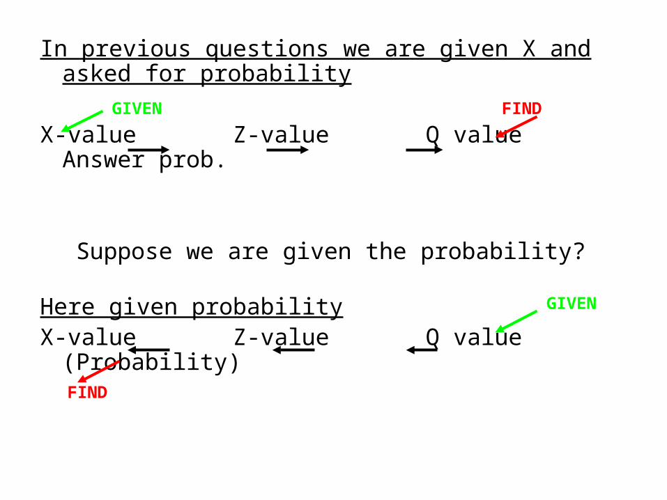
In previous questions we are given X and asked for probability

X-value Z-value Q value Answer prob.

Suppose we are given the probability?

Here given probabilityX-value Z-value Q value (Probability)

GIVEN

GIVEN

FIND

FIND

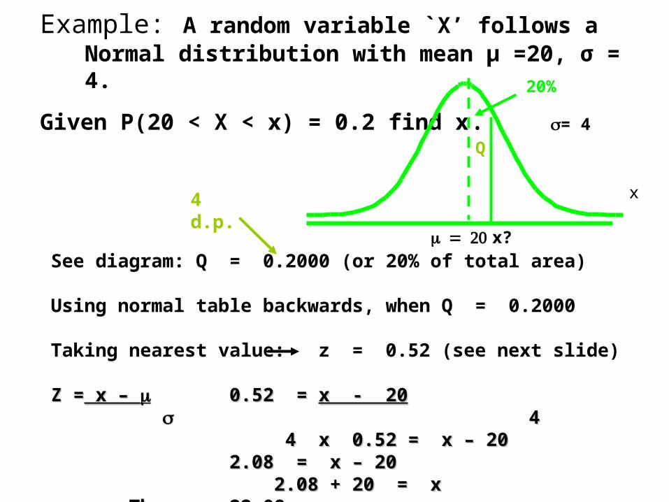
Example: A random variable `X’ follows a Normal distribution with mean µ =20, σ = 4.

Given P(20 < X < x) = 0.2 find x.

Q

See diagram: Q = 0.2000 (or 20% of total area)

Using normal table backwards, when Q = 0.2000

Taking nearest value: z = 0.52 (see next slide)

Z =Z = x – x – 0.52 = 0.52 = x - 20x - 20 44 4 x 0.52 = x – 204 x 0.52 = x – 20

2.08 = x – 202.08 = x – 20 2.08 + 20 = x Thus x = 2.08 + 20 = x Thus x = 22.0822.08

= 4

x?

x4 d.p.

20%

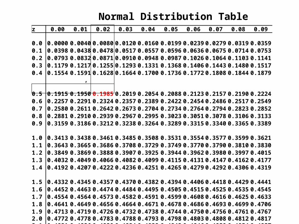
z 0.00 0.01 0.02 0.03 0.04 0.05 0.06 0.07 0.08 0.09

0.0 0.0000 0.0040 0.0080 0.0120 0.0160 0.0199 0.0239 0.0279 0.0319 0.03590.1 0.0398 0.0438 0.0478 0.0517 0.0557 0.0596 0.0636 0.0675 0.0714 0.07530.2 0.0793 0.0832 0.0871 0.0910 0.0948 0.0987 0.1026 0.1064 0.1103 0.11410.3 0.1179 0.1217 0.1255 0.1293 0.1331 0.1368 0.1406 0.1443 0.1480 0.15170.4 0.1554 0.1591, 0.1628 0.1664 0.1700 0.1736 0.1772 0.1808 0.1844 0.1879

0.5 0.1915 0.1950 0.1985 0.2019 0.2054 0.2088 0.2123 0.2157 0.2190 0.22240.6 0.2257 0.2291 0.2324 0.2357 0.2389 0.2422 0.2454 0.2486 0.2517 0.25490.7 0.2580 0.2611 0.2642 0.2673 0.2704 0.2734 0.2764 0.2794 0.2823 0.28520.8 0.2881 0.2910 0.2939 0.2967 0.2995 0.3023 0.3051 0.3078 0.3106 0.31330.9 0.3159 0.3186 0.3212 0.3238 0.3264 0.3289 0.3315 0.3340 0.3365 0.3389

1.0 0.3413 0.3438 0.3461 0.3485 0.3508 0.3531 0.3554 0.3577 0.3599 0.36211.1 0.3643 0.3665 0.3686 0.3708 0.3729 0.3749 0.3770 0.3790 0.3810 0.38301.2 0.3849 0.3869 0.3888 0.3907 0.3925 0.3944 0.3962 0.3980 0.3997 0.40151.3 0.4032 0.4049 0.4066 0.4082 0.4099 0.4115 0.4131 0.4147 0.4162 0.41771.4 0.4192 0.4207 0.4222 0.4236 0.4251 0.4265 0.4279 0.4292 0.4306 0.4319

1.5 0.4332 0.4345 0.4357 0.4370 0.4382 0.4394 0.4406 0.4418 0.4429 0.44411.6 0.4452 0.4463 0.4474 0.4484 0.4495 0.4505 0.4515 0.4525 0.4535 0.45451.7 0.4554 0.4564 0.4573 0.4582 0.4591 0.4599 0.4608 0.4616 0.4625 0.46331.8 0.4641 0.4649 0.4656 0.4664 0.4671 0.4678 0.4686 0.4693 0.4699 0.47061.92.02.1

0.47130.47720.4821

0.47190.47780.4826

0.47260.47830.4830

0.47320.47880.4834

0.47380.47930.4838

0.47440.47980.4842

0.47500.48030.4846

0.47560.48080.4850

0.47610.48120.4854

0.47670.48170.4857

Normal Distribution Table

Summary

• We have revised Normal distribution;

• We have looked at a few problems which involve this type of probability distribution.

• For your tutorial, first - complete Sections A and B from last week

• Then complete the new tutorial sheet before completing Section C from last week