Embed Size (px)
Citation preview

NORTHWESTERN UNIVERSITY
Geometric Aspects of Mixing and Segregation in Granular Tumblers
A DISSERTATION
SUBMITTED TO THE GRADUATE SCHOOL
IN PARTIAL FULFILLMENT OF THE REQUIREMENTS
for the degree
DOCTOR OF PHILOSOPHY
Field of Chemical Engineering
By
James F. Gilchrist
EVANSTON, ILLINOIS
June 2003

ii
© Copyright by James F. Gilchrist 2003
All Rights Reserved
iii
ABSTRACT
Geometric Aspects of Mixing and Segregation in Granular Tumblers
James F. Gilchrist
Recently, much attention has been given to granular systems due to their
widespread use in industrial processes and their often baffling physical behavior. In the
midst of the emerging field of complex systems, granular materials are quickly becoming
a prototypical system exhibiting spontaneous organization. Flowing or vibrated mixtures
of granular materials, differing in physical properties such as size or density,
spontaneously segregate. Constitutive equations describing the behavior of granular
materials, analogous to the Navier-Stokes equations, do not exist. This field, as
compared to fluids, is poorly understood.
Mixing in fluids may be enhanced by the addition of time-periodic perturbations
to the flow, generating chaos. This same concept is applied to granular flow in a tumbler.
A simple two-dimensional continuum model developed by Khakhar et al. 1997b
describing continuous flow in a circular cross section of a tumbler is modified to describe
flow in noncircular geometries. Time-periodic flow in a square is chaotic and sensitive to
fill level. When bi-disperse materials are tumbled in a square, there is direct competition
between mixing and segregation, and pattern formation is nontrivial – segregation
resembles invariant structures of the underlying flow. This model is extended to describe

iv
flow in a sphere and a cube to shed light on the interplay between segregation and chaotic
flow in three-dimensions.
The competition between granular mixing and segregation is also investigated in a
novel spherical tumbler capable of undergoing independent programmed motions in two
orthogonal directions. The primary mode of operation is a combination of rotating and
rocking of the axes. Space-time plots are used to compare experimental results with
surface Poincaré sections obtained using a continuum model of the flow. A phase plot
showing modes of segregation – band formation/no axial bands – in the
frequency/amplitude domain is used to organize the experimental results; segregated
bands are remarkably robust and survive rocking amplitudes of as much as 60 degrees.
Details differ, but the phenomenon occurs both in dry materials and under slurry
conditions.

v
ACKNOWLEDGEMENTS
The following people greatly supported me in my endeavors:
First, I am thankful for the guidance, support and inspiration of my advisor, Professor
Julio M. Ottino. His work in chaotic mixing drew me to graduate school at Northwestern
University, and his ongoing creative approach to research inspired me to pursue an
academic career.
I greatly appreciate the advice and opportunities given to me by my undergraduate
advisors, Professors P. A. Ramachandran and Curt Thies, and that of my co-opportunity
mentor, David Sextro. I also greatly value the conversations with and much valued
advice I received from Professors Devang Khakhar, Rich Lueptow, Seth Lichter, Mary
Silber, Paul Umbanhowar, Bill Cohen, Vassily Hatzimanikatis, and Luis Amaral, each
challenging me to approach my work from different perspectives.
I also appreciate the friendship and support of the members of the Ottino Lab throughout
the years, including Gerald Fountain, Joseph McCarthy, Paul DeRoussel, Marc Horner,
Kurt Smith, (Kats Miyake), Kimberly Hill, Nitin Jain, Peter Andresén, Stanley Fiedor,
Stephen Cisar, Steve Meier, and Ashley Smart.
I thank my family for their love and support, as always. Most of all, I thank my wife, the
love of my life, who believes I can achieve more than I could ever dream.

vi
For Lisa
vii
TABLE OF CONTENTS
Abstract............................................................................................................................. iii
List of Figures................................................................................................................... ix
1 Introduction.................................................................................................................1
2 Kinematics of Mixing in 2D and 3D containers .......................................................5
2.1 Introduction.......................................................................................................5
2.2 2D Tumblers .....................................................................................................8
2.2.1 Model of a Circular Tumbler ..............................................................8
2.2.2 Model of a Noncircular Tumbler ......................................................14
2.2.3 Mixing in a Square............................................................................19
2.3 Extension to Three-dimensional Flow ............................................................33
2.3.1 Geometry and Bi-axial Protocol ....................................................33
2.3.2 Kinematics of a Bi-axially Rotated Sphere and Cube ...................37
3 Competition Between Mixing and Segregation in 2D and 3D containers............45
3.1 Modeling Inter-particle Interactions ...............................................................45
3.1.1 Collisional Diffusion......................................................................45
3.1.2 Segregation ....................................................................................47
3.2 Experimental Details.......................................................................................51
3.2.1 Quasi-two Dimensional Experiments ............................................51
3.2.2 Three-dimensional Bi-axial Experiments ......................................54
3.3 Mixing and Segregation in a Quasi-two Dimensional Tumbler .....................59

viii
3.3.1 Chaotic Mixing with Diffusion......................................................59
3.3.2 Competition between Segregation and Chaotic Advection ...........67
3.4 Segregation in a Sphere and Cube: Bi-axial Rotation ....................................73
4 Flow in a Rotating-Rocking Sphere ........................................................................87
4.1 Model ..............................................................................................................87
4.2 Quasi-Periodic and Chaotic Path-lines ...........................................................93
4.3 Poincaré Maps.................................................................................................97
4.4 Flow Bifurcations..........................................................................................101
5 Rocking Spherical Tumbler ...................................................................................109
5.1 Axial Segregation in Various Geometries ....................................................109
5.2 Experimental Details.....................................................................................116
5.3 Formation of a Band and Spots.....................................................................121
5.4 Space-time Plots............................................................................................123
5.5 Phase Diagram ..............................................................................................127
5.6 Comparison to Computations .......................................................................135
5.7 Granular Slurries ...........................................................................................143
5.8 Rocking Cubes ..............................................................................................148
6 Summary and Outlook ...........................................................................................153
References.......................................................................................................................156
Appendix A ....................................................................................................................161

ix
LIST OF FIGURES
1.1 Examples of organization in granular systems ........................................................3
2.1 Schematic view of flow regimes in a rotating cylinder ...........................................6
2.2 Flow in a circle.........................................................................................................9
2.3 Stretching of a passive blob in a circle ..................................................................11
2.4 Dependence of circulation time on a, 0δ , and h in a circle ...................................13
2.5 Symmetric rotation of a circle at h = 0 and h = 0.5 ...............................................15
2.6 Random-shaped tumbler ........................................................................................16
2.7 Computed streamlines for a half-full circle and square .........................................20
2.8 Two trajectories within a square ............................................................................21
2.9 Poincaré map of a half-full circle and square ........................................................22
2.10 Blob advection and perimeter growth in a circle and square.................................24
2.11 Poincaré maps of the square with filling near half-full..........................................26
2.12 Sensitivity of filling with respect to 0δ .................................................................27
2.13 Mixing in a square, 22.5%-50% full ( 0.055.0 <<− h ) ........................................29
2.14 Mixing in a square, 50%-72.5% full ( 55.00.0 << h )............................................30
2.15 Poincaré maps and mixing of a blob in ¼ and ¾ full square.................................32
2.16 Half-full rotating sphere.........................................................................................35
2.17 Streamline crossing, coordinates and flow in a bi-axially rotated sphere..............36
2.18 Coordinates relative to a bi-axially rotated cube ...................................................38

x
2.19 Schematic diagram of periodic points in a bi-axially rotated sphere.....................39
2.20 Regular regions in a bi-axially rotate sphere .........................................................41
2.21 Schematic diagram of periodic points in a bi-axially rotated cube........................43
2.22 Regular regions in a bi-axially rotated cube ..........................................................44
3.1 Effect of diffusion on a passive blob .....................................................................48
3.2 Quasi-two dimensional apparatus ..........................................................................52
3.3 Three-dimensional tumbler and rotation protocol .................................................55
3.4 Blob experiments and computations......................................................................60
3.5 Mixing of tracer particles in a square ....................................................................61
3.6 Intensity of segregation vs. mixer rotation of tracer particles in a square .............62
3.7 Computations of intensity of segregation vs. mixer rotation for mixers of different
shapes and sizes: top-bottom initial condition.......................................................64
3.8 Computations of intensity of segregation vs. mixer rotation for mixers of different
shapes and sizes: left-right initial condition...........................................................65
3.9 Segregation in half-full circle and square ..............................................................68
3.10 Segregation pattern in a square with different fillings...........................................70
3.11 Bottom view of a cube after 6 and 50 rotations .....................................................74
3.12 Bottom view of an long tumbler with square cross section ...................................75
3.13 Computation of segregation in bi-axially rotated sphere.......................................78
3.14 Experiments in bi-axially rotated sphere ...............................................................79

xi
3.15 Depiction of predicted possible outcomes in the bi-axially rotated cube ..............81
3.16 Computations of segregation in bi-axially rotated cube ........................................83
3.17 Comparison of an bi-axially rotated S-system and D-system with computations .84
4.1 Rocking protocol and coordinates .........................................................................88
4.2 Surface velocities at the mid section of the free surface........................................91
4.3 Relationship between rocking angle and instantaneous flow direction .................92
4.4 Sphere rotating on angle without rocking..............................................................94
4.5 Typical chaotic path-line........................................................................................95
4.6 Typical quasi-periodic path-line ............................................................................96
4.7 Time evolution of the radius of a quasi-periodic and a chaotic trajectory.............98
4.8 Variety of different Poincaré maps in the A-f plane ............................................100
4.9 Concentric Poincaré maps....................................................................................102
4.10 Bifurcation of regular regions (�45=A , 6175.05775.0 << f ). ......................103
4.11 Bifurcation of regular regions (�45=A , 795.07875.0 << f ) ...........................105
4.12 Evolution of the system at �45=A and 968.0953.0 ≤≤ f ................................106
4.13 Evolution of the system in region of �60=A and 960.0930.0 ≤≤ f ................108
5.1 Tumblers of different geometry ...........................................................................111
5.2 Self-organization of axial bands in a slurry .........................................................112
5.3 Axial segregation observed in a tumbler with square cross section ....................114
xii
5.4 Formation of an axial band in a sphere................................................................117
5.5 Experimental setup and rocking protocol ............................................................118
5.6 Segregation patterns in a rotating-rocking sphere ..............................................122
5.7 Spatio-temporal plots of classic axial segregation...............................................124
5.8 Construction of spatio-temporal composite images.............................................126
5.9 Evolution of the Froude number as a function of frequency and amplitude .......128
5.10 Series of experiments at A = 45º ..........................................................................129
5.11 Experimental phase diagram................................................................................131
5.12 Qualitative comparison of experimental and frequency-locking phase
diagrams...............................................................................................................134
5.13 Comparison between a band and computed quasi-periodic trajectories ..............137
5.14 Comparison between regular regions in model and spots in experiments...........138
5.15 Transition between a band and spots in experiment compared to the model ......140
5.16 Experiments under slurry conditions ...................................................................144
5.17 Odd patterns under slurry conditions...................................................................146
5.18 Model and slurry experiment displaying period-6 periodic points......................147
5.19 Rocking cube with f = 1 .......................................................................................150
5.20 Rocking cube with f ~ 0.8 ....................................................................................151
A.1 Computations of a rocking sphere for A = 5º and .5 � f < 1.5 .............................162
A.2 Computations of a rocking sphere for A = 10º and .5 � f < 1.5 ...........................163

xiii
A.3 Computations of a rocking sphere for A = 15º and .5 � f < 1.5 ...........................164
A.4 Computations of a rocking sphere for A = 20º and .5 � f < 1.5 ...........................165
A.5 Computations of a rocking sphere for A = 25º and .5 � f < 1.5 ...........................166
A.6 Computations of a rocking sphere for A = 30º and .5 � f < 1.5 ...........................167
A.7 Computations of a rocking sphere for A = 35º and .5 � f < 1.5 ...........................168
A.8 Computations of a rocking sphere for A = 40º and .5 � f < 1.5 ...........................169
A.9 Computations of a rocking sphere for A = 42.5º and .5 � f < 1.5 ........................170
A.10 Computations of a rocking sphere for A = 45º and .5 � f < 1.5 ...........................171
A.11 Computations of a rocking sphere for A = 47.5º and .5 � f < 1.5 ........................172
A.12 Computations of a rocking sphere for A = 50º and .5 � f < 1.5 ...........................173
A.13 Computations of a rocking sphere for A = 52.5º and .5 � f < 1.5 ........................174
A.14 Computations of a rocking sphere for A = 55º and .5 � f < 1.5 ...........................175
A.15 Computations of a rocking sphere for A = 60º and .5 � f < 1.5 ...........................176
A.16 Computations of a rocking sphere for A = 70º and .5 � f < 1.5 ...........................177

1
CHAPTER 1
INTRODUCTION
Recently, much attention has been given to granular systems due to their
widespread use in industrial processes and their often baffling physical properties.
Granular processes are found widely in nature in processes such as dune formation,
sediment deposits in river deltas, and also in catastrophic events such as landslides.
Granular-flow studies have recently received substantial attention within the physics and
engineering communities (Jaeger et al. 1996a, b, Jaeger & Nagel 1992, Bridgewater
1995). Despite this recent attention, the dynamics of granular materials is still poorly
understood when compared to fluids. There are no constitutive equations analogous to
the Navier-Stokes equations in fluids capable of describing general behavior of granular
flow. Most industrial mixing applications are approached on an ad hoc basis, often with
significant complications. Scale-up of laboratory-scale processes is often impossible.
The behavior of most systems cannot be predicted outside their operating parameters.
At the same time, granular materials are quickly becoming a prototypical system
in the emerging field of complex systems. A complex system may be loosely defined as a
large number of interactive constituents or agents capable of exhibiting spontaneous
organization. For instance, vibrated granular beds exhibit complex pattern formation and
can spontaneously organize into coherent structures known as oscillons (figure 1.1 top)
and other lattice-like structures (Umbanhowar et al. 1996). Also, flowing mixtures of
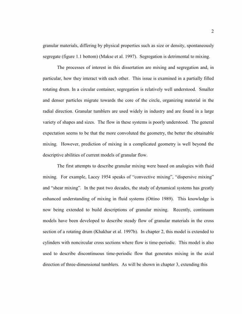
2
granular materials, differing by physical properties such as size or density, spontaneously
segregate (figure 1.1 bottom) (Makse et al. 1997). Segregation is detrimental to mixing.
The processes of interest in this dissertation are mixing and segregation and, in
particular, how they interact with each other. This issue is examined in a partially filled
rotating drum. In a circular container, segregation is relatively well understood. Smaller
and denser particles migrate towards the core of the circle, organizing material in the
radial direction. Granular tumblers are used widely in industry and are found in a large
variety of shapes and sizes. The flow in these systems is poorly understood. The general
expectation seems to be that the more convoluted the geometry, the better the obtainable
mixing. However, prediction of mixing in a complicated geometry is well beyond the
descriptive abilities of current models of granular flow.
The first attempts to describe granular mixing were based on analogies with fluid
mixing. For example, Lacey 1954 speaks of “convective mixing”, “dispersive mixing”
and “shear mixing”. In the past two decades, the study of dynamical systems has greatly
enhanced understanding of mixing in fluid systems (Ottino 1989). This knowledge is
now being extended to build descriptions of granular mixing. Recently, continuum
models have been developed to describe steady flow of granular materials in the cross
section of a rotating drum (Khakhar et al. 1997b). In chapter 2, this model is extended to
cylinders with noncircular cross sections where flow is time-periodic. This model is also
used to describe discontinuous time-periodic flow that generates mixing in the axial
direction of three-dimensional tumblers. As will be shown in chapter 3, extending this
3
Figure 1.1: Examples of self-organization in granular systems. Top – vibrated
materials spontaneously coordinate into coherent structures such as “oscillons”
(Umbanhowar et al. 1996). Bottom – mixtures of flowing granular materials, differing
by physical properties such as size, spontaneously segregate into bands as they are
poured to form a heap (Makse et al. 1997).

4
model further with the addition of collisional diffusion and segregation due to buoyancy
allows description of systems consisting of mono-disperse and bi-disperse materials.
The result of the mixing-segregation interaction is nontrivial. The segregation
patterns predicted by this model are compared to patterns produced in experiments in
both quasi-two dimensional tumblers and in a sphere and a cube rotated to produce three-
dimensional flow. This is examined in experiments of both S-systems (size segregation)
and D-systems (density segregation). Experiments in a sphere and a cube are conducted
under dry and slurry conditions (where air is completely replaced by a more viscous
fluid). Non-invasive techniques are used to visualize the shape of segregated structures.
Experimental studies in rocking cylinders suggest that mixing is enhanced by the
incorporation of axial advection (McCarthy et al. 1996, Wightman et al. 1998a). Chapter
4 considers mixing in a rotating-rocking sphere where mixing is found to be sensitive to
both the amplitude and frequency of rocking. Chapter 5 examines an experimental
realization of this system, presenting direct comparisons between segregation patterns in
the sphere experiments under both dry and slurry conditions.

5
CHAPTER 2
KINEMATICS OF MIXING IN 2D AND 3D CONTAINERS
This chapter extends the 2D model derived by Khakhar et al. 1997b for
mixing in a circle to convex geometries and 3D containers. The main
focus is to understand, from a continuum perspective, how chaotic
advection affects mixing. Chaos may be produced by changing the tubler
geometry, changing the degree of filling, and introducing flow in three-
dimensions.
2.1 Introduction
Flow in a rotating cylinder is well defined and can be classified into different
regimes (Henein et al. 1983, Rajchenbach 1990). These regimes are depicted in figure
2.1. At low rotational speeds (quantified in terms of the Froude number, gLFr /2ω= ,
where g is the acceleration due to gravity, L is the length scale of the system, and ω is
the rotational speed), the flow occurs as discrete avalanches; one avalanche stops before
the next one begins (this is the so-called avalanching or slumping regime). A simple
geometrical model describes overall flow (Metcalfe et al. 1995). Material rotates as a
solid body until the free surface reaches a critical angle, at which the material flows and
then comes to rest. Each avalanche comprises of a wedge of particles near the free

6
Fig
ure
2.1
: S
chem
atic
vie
w o
f fl
ow
reg
imes
in a
rota
ting c
yli
nder
wit
h i
ncr
easi
ng r
ota
tional
spee
d,
ω.
In t
he
aval
anch
ing r
egim
e, t
he
das
hed
lin
e sh
ow
s th
e posi
tion o
f th
e in
terf
ace
afte
r an
aval
anch
e as
the
mat
eria
l re
lax
es f
rom
th
e m
axim
um
an
gle
of
rep
ose
, β i
, to
the
final
angle
of
repose
, β
f. T
he
angle
β i
n
the
roll
ing
reg
ime
is t
he
dynam
ic a
ngle
of
repose
.

7
surface, transported from the upper to the lower part of the container. Mixing occurs
within the wedge and across intersections of consecutive wedges. Geometry and fill level
have significant impact, especially when geometrical features of the tumbler are
asymmetric (such as baffles considered in McCarthy et al. 1996).
At higher speeds a steady flow is obtained with a thin cascading layer at the free
surface of the rotating bed (this is the continuous flow regime, also known as the rolling
or cascading regime). The free surface is nearly flat. At still higher speeds, particle
inertia effects become important, causing the free surface to form an “S” shape and
particles become airborne (cataracting regime). There are many different models that
describe flow in both the rolling and cataracting regime based on assumptions derived
from experimental observations. 1=Fr roughly corresponds to the critical speed for
centrifuging where material only rotates solid body and no mixing occurs. Flow is more
complicated when tumbling cohesive particles or mixtures of particles differing in
physical properties (for instance, size). From here on, only the continuous flow or rolling
regime is considered. The particles will range in size from 0.2 mm to 3 mm diameters.
Cohesion is not an issue.
Some of the important features of flow in the rolling regime are revealed using
NMR (Nakagawa et al. 1993). The flowing layer is fluidlike and the velocity profile is
nearly linear. Rajchenbach et al. 1995 show similar results near the midpoint of the
flowing layer for a two-dimensional system. More recently, a more detailed study
analyzes the velocity profiles across the entire layer for different rotation rates and bead
sizes (Jain et al. 2002). They find that the streamwise velocity profile scales along the

8
free surface as ( )( )[ ]22 /1/ LxLu −ωδ where ω is the rotation rate, u is the average
velocity, δ is the local depth of the flowing layer, and x is the position along the free
surface ( 0=x is the midpoint and the free surface is 2L long – see figure 2.2). Jain et al.
2003 also include variation of the interstitial fluid properties (replacing air with water),
finding similar results.
The next section builds on the model developed by Khakhar et al. 1997b
describing flow in two-dimensional circle in the rolling regime. This model uses the
following assumptions (based on experimental results):
1) The shear profile along the layer is linear.
2) The free surface is flat.
3) Material rotates as a solid body beneath the flowing layer.
Additions to this model describing collisional diffusion and segregation are incorporated
in chapter 3.
2.2 2D Tumblers
2.2.1 Model of a circular tumbler
Consider a circular tumbler, as shown in figure 2.2. The circle is rotated about its
center, denoted C. The free surface is flat and the filling is measured by h, the distance of
the free surface from C. There are two regions of flow. Most material rotates as a solid
body without slip. Near the free surface, material is convected by a rapid shear flow.
Coordinates associated with this flow are at the center of the free surface, O. A thin

9
Figure 2.2: Flow in a circle partially full of material (light gray region, here shown as
both half-full and more than half-full with height h) and rotated clockwise about the
center of the circle at constant rate, ω . All material is in solid body rotation except a thin
region near the free surface. The boundary between solid body rotation and shear flow is
denoted as ( )xδ . Variables in the model are scaled by ω and L, the half-length of the
free surface, and the coordinate system is centered on the free surface. Trajectories
follow along closed streamlines, shown as dotted lines. When more than half-full, the
circle forms an unmixed core at the center (dark gray circular region shown on right).

10
boundary layer of thickness ( )2
0 1 x−= δδ (spatial variables are made dimensionless
with L, the half-length of the free surface) separates solid body rotation from shear flow
(Khakhar et al. 1997b). The maximum depth of the flowing layer, 0δ , is estimated from
experiments, and ranges roughly from 0.03 to 0.10.
A general form for the velocity field of the rapid shear flow that conserves mass
in the flowing layer is
���
����
�−+=
a
xy
aauv
δ1
1 (2.1)
1+
��
���
�−=a
yyxvδ
(2.2)
Time is scaled with respect to ω/1 . The average velocity is ( )02/1 δ=u . In this
generalized form, 1=a corresponds to a linear profile, 2/3=a is refered to as the
Bagnold profile (Bagnold, 1954), and ∞=a is plug flow. For any value of a, this model
produces closed streamlines (shown as dotted lines in figure 2.2). Particle motion along
these streamlines is calculated by integrating the above velocity equations in the layer
and rotating solid body in the bed. Particles spend much more time in solid body rotation
than in the flowing layer.
Consider a passive blob of material passing through the flowing layer (figure 2.3).
This blob consists of about 104 closely spaced particles. As it enters the layer, it is
stretched by the shear flow and then exits into the solid-body region. The net effect is

11
Figure 2.3: Stretching of a passive blob of 104 particles (colored gray and black). Top –
time evolution of a blob of tracer particles as it moves through the flowing layer. As
material passes through the layer, it rotates 180� and stretches in the θ -direction. Bottom
– the same blob after 20 rotations stretches and connects through the flowing layer (initial
condition in gray). The angle of repose is arbitrary. For convenience, the free surface is
shown as horizontal.

12
stretching in the θ -direction and 180° rotation of the blob. At the bottom of figure 2.3,
the mixing pattern is shown in a half-full circle after 20 rotations.
The distribution of circulation times for the closed streamlines (time of one
revolution about each streamline) is given by ( )rTC . Plots in figure 2.4 show the effect
of a, 0δ , and h on ( )rTC . The velocity profiles with a ranging from 2/3 to 3/2 are
depicted in figure 2.4a. To calculate CT , a straight line of initial conditions in the radial
direction is advected, and the time for a particle at distance r to return to its initial
position is recorded. The circulation times are almost independent of the parameter a
(figure 2.4b). Because of this, mixing occurs in the same manner and at nearly the same
rate for all velocity profiles considered. Therefore, a simple linear shear, 1=a , is used
from here on.
Figure 2.4c shows that the deviation in circulation times becomes more
pronounced along r for increasing 0δ . For 00 =δ , all trajectories have the same
circulation time and there is no mixing. Also, changing h significantly changes the
circulation times in the tumbler (figure 2.4d). Both the thickness of the layer and the
filling of the tumbler affect the mixing rates significantly more than the form of the
velocity in the layer. Most simulations in this thesis are calculated using 05.00 =δ
unless specified otherwise.
Increasing h does not change the dynamics of the flowing layer, however it causes
particles to spend more time in solid body rotation. This is the reason why h has such a
large effect on the circulation rate. It should also be noted that h is the only parameter in

13
Fig
ure
2.4
: C
ircu
lati
on r
ate,
T(r
).
The
thre
e dif
fere
nt
vel
oci
ty p
rofi
les
are
show
n i
n (
a),
and h
ave
alm
ost
no e
ffec
t on c
ircu
lati
on r
ate
(b).
H
ow
ever
, ci
rcula
tion r
ate
dep
ends
slig
htl
y o
n t
he
dep
th o
f th
e fl
ow
ing
layer
(c)
and g
reat
ly o
n t
he
fill
ing (
d).
14
a physical system that is user-defined. Instead of calculating the circulation rate at each
r, the average circulation time (T*) can roughly be calculated by dividing the time for a
full rotation (in dimensionless variables, π2 ) by the percent filling. For instance, in a
half-full mixer all of the material passes through the layer in ½ rotation (T* = ½). For
more than half-full circles (specifically 0δ>h ), a core of material that never reaches the
flowing layer resides in the center. Because circulation rate depends on r, there is only
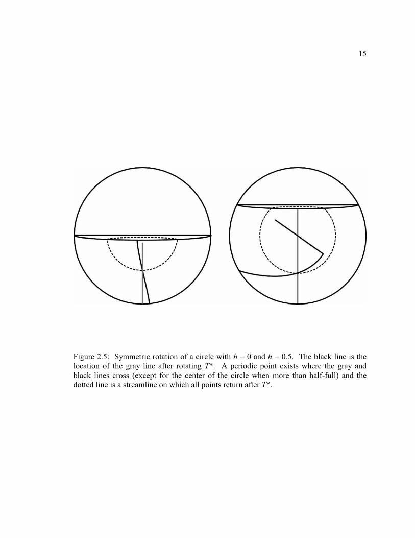
one streamline on which all points return after *Tt = . This is shown in figure 2.5 at
various fillings. An initial line of points is advected for T*. In the half-full case, the
points near the center rotate past their initial locations, whereas points near the boundary
do not pass the original line of points. There is one point that returns exactly to its
original location (corresponding to the crossing of the initial line and the final line of
points). This point and all points on the same streamline are invariant with respect to T*
rotations (so called periodic points). This has little relevance in a circle; however, in
chaotic systems it is the periodic points and regions near these points that define the local
mixing.
2.2.2 Model of a noncircular tumbler
Consider a general, two-dimensional, non-circular tumbler filled to some extent
(figure 2.6). Only convex tumblers are considered to ensure that the free surface only
intersects with the boundaries at only two points. The system is rotated about its
15
Figure 2.5: Symmetric rotation of a circle with h = 0 and h = 0.5. The black line is the
location of the gray line after rotating T*. A periodic point exists where the gray and
black lines cross (except for the center of the circle when more than half-full) and the
dotted line is a streamline on which all points return after T*.

16
Figure 2.6: Irregularly-shaped tumbler. The center of the free surface, O, moves relative
to the centroid, C. This picture is limited to convex tumblers such that the flowing layer
never intersects the container boundaries except at x = -p1 and x = p2. The half-length of
the flowing layer (L), the height (h) and the lateral position of the center of the free
surface (s) are now functions of time.

17
centroid, C, at a constant rate ω ; coordinates are associated with the flowing layer are at
the center of the free surface, O. One can think of a circle as a special case of this system
where the shape of the region of flow is constant. Without this restriction, the flowing
layer changes periodically with rotation. O moves relative to C (except in the case of
half-full and a 180� rotationally symmetric geometry, considered in Khakhar et al.
1999a). Also, the length of the free surface changes with time. Elperin and Vikhansky
1998a also present a description of mixing in various geometries and perform a detailed
analysis of the symmetries for different geometries at various fillings. However, their
billiards-like model does not consider the dynamics within the flowing layer. For
instance, no mixing is predicted in a half-full circle or square. The basic assumptions and
the model described below are also presented in Khakhar et al. 2001a,c as applied to heap
formation, Orpe et al. 2001 as applied to tumbling, and in Khakhar et al. 2001a where the
model is applied to both cases. More recently, the model has been used to scale
experimentally measured velocities in slurries (Jain et al. 2003). Surprisingly, the model
works well even under slurry conditions.
Experiments by Khakhar et al. 1999a show that in different sized circular
containers, the maximum depth of the flowing layer scales with the length of the free
surface. Assume that the layer geometry changes slowly with time compared to the
dynamics of the flow. The flow is then quasi-steady and similar to that for a circle with
the same layer geometry. As discussed in section 2.1, inertial effects of the solid body
rotating particles in the rolling regime are negligible. With these added assumptions, the
velocities in the flowing layer in a noncircular container are

18
( ) ( )( ) ��
�
����
� −+=θδθθ
,12
xhyuLvx (2.3)
( )( ) ( )( )
2
, ���
����
� −−−=θδθθ
xhysxv y (2.4)
As before, these equations are dimensionless with L, now denoted as the half-length of
the free surface at a specified angle, and ω/1 . ( )θh is the dimensionless height of the
free surface at any angle of rotation relative to C (as shown in figure 2.6). The area of the
region of flow under ( )θh remains constant and depends on the initial fill fraction of the
tumbler. ( )θs , the horizontal position of O, is determined by calculating the x-
coordinates p1 and p2 (relative to C) where the free surface intersects the container
boundaries. From this, the lateral location of the center and the half-length of the free
surface are ( ) ( ) 2/12 pps +=θ and ( ) ( ) 2/12 ppL −=θ respectively. The shape of the
flowing layer changes in time as
( ) ( ) ( ) ��
�
�
��
�
����
����
�−=2
0 1,θ
θδθδL
xLx (2.5)
These equations in the layer, with solid body rotation underneath it, describe flow in any
partially full convex container. It should be noted that different functionalities for layer
profiles (e.g., ( )2
0 /1 Lx−= δδ ), give essentially the behavior as described in the next
section, indicating that global aspects (i.e., the shape of the container) control the
important details of the physics.

19
All information about geometry enters into the velocity equations through the
functions ( )θL , ( )θh , and ( )θs , which are time-periodic with each rotation. As
suggested by several studies on fluid mixing, time modulation of a two-dimensional flow,
where superimposed streamlines at different times intersect, is sufficient to produce
chaotic advection. This is demonstrated in figure 2.7 for a half-full square. Closed
streamlines in the circle can be thought of as barriers against transport in the radial
direction. In the square, streamlines associated with two different orientations cross in
the flowing layer. This picture becomes more complex when the square is not half-full.
2.2.3 Mixing in a square
As already suggested in figure 2.3, mixing in a circle is simple. Deformation of
material elements is linear with time. It is also easy to calculate the locations of periodic
points. This is not the case in a square. First consider a half-full square. L in this
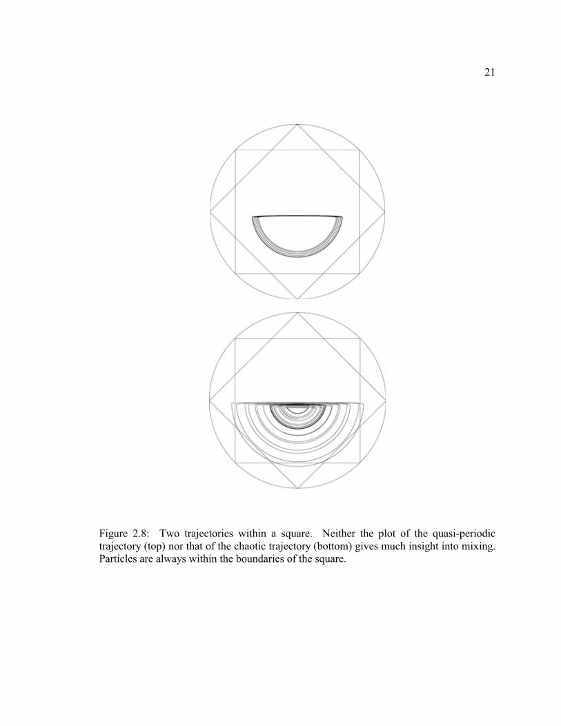
container is taken as half the width of the square. Figure 2.8 shows two particle
trajectories (each for 50 rotations). The large circle represents the maximum width of the
flowing layer (particles never leave the square). The top trajectory appears to be quasi-
periodic, wrapping around on a closed surface. The bottom trajectory appears to
randomly enter and exit the flowing layer.
A Poincaré map is a way to show long-time behavior of initial conditions in
different parts of the flow (figure 2.9). To produce this map, particles are advected and
their locations are plotted at the end of each ½ rotation for 200 rotations (as noted in the

20
Figure 2.7: Computed streamlines for a half-full circle and square. The circle has closed
streamlines that act as barriers to transport in the radial direction. The square is shown at
two different orientations. The shaded region in the square shows where intersections
occur between streamlines associated with each orientation.
21
Figure 2.8: Two trajectories within a square. Neither the plot of the quasi-periodic
trajectory (top) nor that of the chaotic trajectory (bottom) gives much insight into mixing.
Particles are always within the boundaries of the square.

22
Figure 2.9: Poincaré map of a half-full circle and square. In a circle, points are always
located on closed streamlines. In the square, different regions of mixing exist. Regular
regions have quasi-periodic orbits. A chaotic sea exists in the middle where mixing is
enhanced.

23
circle, all half-full containers have an average circulation time of a ½ rotation). Each
color represents a different initial condition. In a circle, the Poincaré map shows only
regular motion (“regular” may be roughly interpreted as the opposite of chaotic), and the
invariant curves obtained coincide with the streamlines. However, in a square, regions of
chaotic motion are interspersed with regions of regular motion. Regular regions with
quasi-periodic orbits exist around elliptical points. In these regions, the mixing that
occurs is analogous to that found in a circle. The “chaotic sea” that surrounds hyperbolic
points is where mixing is enhanced (there are two hyperbolic points, one of which is
located in the flowing layer). KAM surfaces, chains of high periodicity periodic points
that surround the regular regions, act as a barrier to transport.
The differences between mixing in the chaotic region and the regular regions
become apparent when two passive blobs are advected and their positions are plotted
after 20 rotations (figure 2.10 top). Material in the regular region is trapped, only mixing
with material in its vicinity. Material in the chaotic regions is spread throughout a larger
region of the granular bed. The rate of stretching in the chaotic region may be quantified
by tracking the perimeter length of the blob as a function of time (figure 2.10 bottom).
The perimeter of the blue blob in the chaotic region grows exponentially. The blob is
stretched along unstable manifolds of the hyperbolic point. This stretching deforms the
blob into a thin filament which folds back upon itself repeatedly as it follows a
heteroclinic orbit along the stable manifold of the other hyperbolic point. As the blob
approaches the other hyperbolic point, it begins to stretch along an unstable manifold and
the process repeats.

24
Figure 2.10: Blob advection in a square (top) and perimeter growth in a square and circle
(bottom). Material initially located in the regular region is trapped, only mixing locally.
A blob that starts in the chaotic region gets stretched and folded, enhancing mixing. The
length of the perimeter of the blob in the chaotic region increases exponentially with
number of rotations. The same blob in a circle only has linear growth of its perimeter.

25
Consider the symmetries of a square. The square has symmetries such that the
boundaries return to their original location after a ¼ rotation. This means that the
functions ( )θL , ( )θh , and ( )θs are periodic with every ¼ rotation. This suggests that
drastic changes may occur in the square for ¼, ½ and ¾ fillings (corresponding to
average circulation times of 2/π , π , and 2/3π ). The regular regions in the half-full
square are associated with periodic points that return every half-rotation. Consider the
system when it is slightly more or less than half-full. The average circulation time
increases with increasing h. Therefore, when the container is not half-full, no points can
return to their original location after just ½ rotation. The Poincaré maps for
1.01.0 <<− h are shown in figure 2.11. Beginning at half-full, with increasing h the
regular regions migrate toward the center of the tumbler and shrink until they disappear.
All that remains is chains of high period periodic points (KAM surfaces) that inhibit
transport in the radial direction. With decreasing h, the regular regions also shrink as
they move toward the outer corners of the square. Once again, eventually only KAM
surfaces remain. When KAM surfaces exist, the topology is very similar to the circle.
Clearly, the topology of the flow is extremely sensitive to fill level.
Recall that in a circle the distribution of circulation times is broader for larger
values of 0δ . In the square, the effects are as follows (figure 2.12). When 0δ is small,
small changes in h cause the regular regions to disappear. When 0δ is deeper, the

26
Figure 2.11: Poincaré maps of the square with filling near half-full. From half-full,
increasing h causes the regular regions to migrate toward the center and shrink. With
decreasing h, the regions shrink as they migrate toward the boundaries. The topology of
the underlying flow at 45% and 55% full are similar, both consisting mainly of KAM
surfaces that inhibit transport in the radial direction.

27
Figure 2.12: Sensitivity of topology to filling for different 0δ . Top – the radial position
of the regular regions seen at half-full is dependent on h. Here, positions are plotted for
different layer depths ( 2 is the length of the diagonal from center of the square to the
corner). Bottom – the rate at which these regular regions disappear is inversely
proportional to 0δ .

28
topology of the flow is insensitive to fill level. The position of the regular region, r*, is
plotted as a function of changing h for different values of 0δ . Plotting the slopes of these
lines shows that the rate of this transition is inversely proportional to 0δ . This suggests
that if the depth of the flowing layer is very thin, mixing is very sensitive to the fill level.
Therefore, any error in measuring fill level translates as a large effect on mixing. Small
deviations in fill level within a noncircular tumbler can result in significantly different
mixing.
Figure 2.13 shows Poincaré maps from 0.055.0 <<− h . As one decreases h, first
the topology primarily consists of high period chains of islands. The periodicity of the
chains in each map decreases with smaller fillings. At less than 35% full, most of these
chains are destroyed, apparently leaving only period 2, 3 and 4 islands. The rest of this
map appears chaotic. 5.0−=h corresponds to a symmetric filling with respect to the
square (25% full). Here, a single island passing through the layer exists. The shape of
this island is different than previous regular regions. Instead of an elliptical point, the
periodic point in this island is hyperbolic. Analogous to less than half-full, multiple
bifurcations occur in the range 55.00 << h (figure 2.14). With increasing filling, the
regular regions disappear, and chains of high period periodic points form and migrate
outward. A diamond shaped core appears in the center. The same type of regular regions
seen at 5.0−=h also forms at 5.0=h . Only one of three regions is stretched through the
layer in this map, and it is apparent that these regions are not centered about elliptical
points.

29
Figure 2.13: Mixing in a square, 22.5%-50% full ( 0.055.0 <<− h ). The flow goes
through multiple bifurcations with changing h. Regions of poor mixing form near 25%
and 50% full (symmetric fillings).

30
Figure 2.14: Mixing in a square, 50%-72.5% full ( 55.00.0 << h ). Regions of poor
mixing form around 50% and 75% full (symmetric fillings). A core region exists for all
fillings where 05.0>h .

31
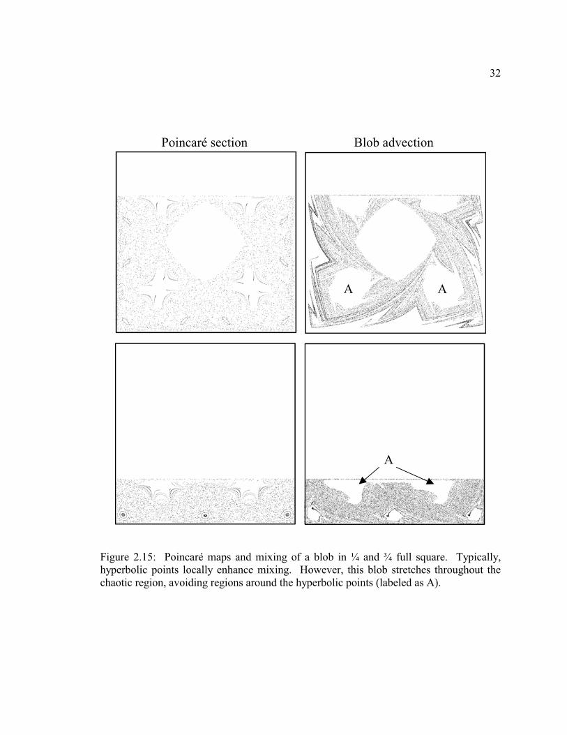
At half-full, a hyperbolic point is centered in the chaotic region. At ¼ and ¾ full,
it appears as if there are hyperbolic points; however mixing in these regions is poor
(figure 2.15). A blob that starts in the chaotic region stretches and folds to eventually
spread throughout the chaotic region. However, material from this blob never infiltrates
into the regions near the hyperbolic points. Flow in these regions is as follows. In the ¼
full case, as material near a hyperbolic point passes through the flowing layer, it is
stretched along unstable manifolds and rotated 180�. This material then solid body
rotates ¼ rotation until it begins to enter the layer once again. The net rotation of this
material as it re-enters the flowing layer is 270�, unlike the half-full case where a blob in
the regular regions rotates 360� (180� from solid body rotation and 180� while passing
through the flowing layer). Once again, material stretches along the unstable manifolds
as it passes through the flowing layer. However, this acts to deform this material to its
original shape (90� rotation is the same as reversing the stability of each eigenvector).
Every two passes through the layer results in 180� rotation of material without stretching.
The same occurs in the ¾ full square; however, material rotates 450� with each ¾ rotation
of the square. In this region, no mixing occurs.
It is clear that variations in geometries give rise to drastically different mixing
topologies. However in each system, the combined symmetries of both the container and
the degree of filling dictate how mixing occurs. For instance, a triangle (and any odd
number regular polygon) is not symmetric to ½ rotations. However, it is expected that
when a triangle is 1/3 or 2/3 full, regular regions will form in the corners as seen in the
square. Thus far, only mixing in the cross section of an elongated drum is considered.
32
Figure 2.15: Poincaré maps and mixing of a blob in ¼ and ¾ full square. Typically,
hyperbolic points locally enhance mixing. However, this blob stretches throughout the
chaotic region, avoiding regions around the hyperbolic points (labeled as A).
Poincaré section Blob advection
A A
A

33
Another way to introduce time-periodicity into the system is to change the direction of
flow, producing flow along the axis of rotation. As described in the next section, the
above models can also be used to describe discontinuous flow in certain three-
dimensional geometries.
2.3 Extension to Three-Dimensional Flow
2.3.1 Geometry and bi-axial protocol
The above model considers only 2D flow in a cross section. However, if applied
to a longer container, it does not imply that different cross sections along the axis of
rotation must be identical. For instance, a circle can either be a cross section of a
cylinder or a sphere. This can be extrapolated for many different shapes as long as the
geometry does not induce flow across each plane of flow. For this to be true, each cross
section along the axis must have constant area under the free surface. Assume that the
flow scales by the local length of the free surface in each cross section in the direction of
flow and neglects any effect of shear in the axial direction. In the actual system, this
assumption may not be accurate, especially considering end-effects that arise in
experiments in almost all rotating cylinders.
With this additional assumption, the model described above may be used to model
flow in noncylindrical geometries. The length of the free surface now depends on axial
position ( ( )zLL = , where z points orthogonal to x and y-directions). In the rolling
regime, the free surface is a flat plane. However, based on experimental results, the free

34
surface is not necessarily flat (Zik et al. 1994). In a container where the radius varies
sinusoidally in the z-direction, they report that geometry slightly changes the angle of
repose. Also, Elperin and Vikhansky 2000 model the shape of the free surface in an
ellipsoid with flow in the axial direction.
Consider flow in a half-full sphere (figure 2.16). The free surface is a circular
plane and steady flow in each cross section scales as ( ) 21 zzL −= (dimensionless with
radius). We assume that each cross section behaves as described above where particles
move along closed streamlines. As is seen in noncircular tumblers, periodic modulation
of the flow can enhance mixing by inducing chaos. This is straightforward in a sphere.
Imagine rotating for a given amount of time, stopping and then rotating on a different
axis. Cycling between the two axes causes streamlines associated with the each flow
direction to cross each other in the flowing layer (figure 2.17 top). Changing directions
of the flow is simply modeled by translating particles to the new coordinate system
associated with rotation on an alternate horizontal axis. The flow is assumed to start and
stop instantaneously and rotation that does not produce a flowing layer is neglected.
The parameters in this system are the number of axes of rotation, the angle
between axes, the amount of rotation about each axis, and the order of rotations about
different axes. One can imagine a scheme to describe this parameter space and the
symmetries (similar to the symmetry analysis by Franjione and Ottino 1992). Consider a
simple protocol of two-axis rotation as shown at the bottom right of figure 2.17. The
axes are orthogonal with a rotation of π=T about each axis; this is referred to as the

35
Figure 2.16: Half-full rotating sphere. The velocity on the surface scales with the length
of the free surface in the direction of flow. The horizontal axis of rotation is arbitrary,
flow in any direction is identical.

36
Figure 2.17: Top – streamline crossing at the surface, coordinates and flow in a bi-
axially rotated sphere. Flow associated with rotation about two orthogonal axes is shown
in red and blue. Bottom – the coordinate system for each flow and the protocol depicting
consecutive rotations.
37
“bi-axial” protocol. Obviously, mixing will be different with more involved schemes, but
this can be used as a reference case. A bi-axially rotated sphere may be the simplest
system exhibiting axial transport and chaos.
The same model applies to a bi-axially rotated cube (figure 2.18). The cube is
invariant to rotations of 90� on each axis of rotation face-center on different sides of the
cube. Flow in each cross section is described as flow in a square. Like the sphere, bi-
axial rotation causes advection in the axial direction. Understanding of dynamics in a
circle and a square facilitates the analysis of these two systems.
2.3.2 Kinematics of a bi-axially rotated sphere and cube
As seen in the square, invariant regions describing the underlying flow can be
located in terms of the periodic points of the flow. The location of periodic points in both
the bi-axially rotated sphere and cube can be located by knowing the dynamics of a circle
and square and the symmetries of the bi-axial flow. A qualitative analysis yields
considerable insight. First, consider the sphere. In a half-full circle rotated π=*T , there
exists a single streamline such that all points return to their original location (as depicted
in figure 2.5). This streamline of periodic points is located at r* in the region of solid
body rotation (figure 2.19). Computations indicate that 2/1* ≅r (note: a closed integral
equation can be written by calculating the Hamiltonian for the velocity field; the exact
position of r* is slightly dependent on the depth of the flowing layer, 0δ ). Such a
streamline exists in each axial cross section of flow on each axis, therefore tracing a

38
Figure 2.18: Left – coordinates in a bi-axially rotated cube. Each cross section is
modeled as a square, the dynamics of which are depicted in the Poincaré map on the
right.

39
Figure 2.19: Schematic diagram of periodic points in a bi-axially rotated sphere. In each
cross section, a streamline exists on which points return to their original location after ½
rotation. In the sphere, this creates an invariant surface of periodic points in any direction
of flow, shown on the right for two orthogonal directions of flow.

40
surface of periodic points within the sphere. In each cross section along the z-axis, this
streamline is located at 2/1* 2zr −≅ within that cross section (here, r is relative to the
circle, not spherical coordinates). In Cartesian coordinates, the equation describing this
ellipsoidal surface within the region of solid body rotation is ( ) 4/1 222 zyx −≅+ . This
surface of periodic points exists for rotation in any direction. Therefore, after a ½
rotation on one axis and then a ½ rotation on the orthogonal axis, periodic points exist at
the intersection of this surface and its projection in the orthogonal direction. The
intersection of these two surfaces form two curves in the zx = and zx −= planes at
( ) 221¼ xzy −−≅ .
Seeding initial conditions near these periodic points and advecting them with the
bi-axial flow indicates the local stability of these points. Periodic points located in the
zx −= plane are elliptic. Particles starting near these points are trapped in a regular
region and circulate about a given elliptical point, as shown in figure 2.20. In three-
dimensional flow, this elliptic point has two imaginary eigenvalues and one null
eigenvalue. The points near the elliptic points rotate in a plane orthogonal to the radial
direction. The volume of the regular regions is small compared to the volume of the
sphere. All trajectories outside of the regular regions appear to be chaotic. Periodic
points in the zx = plane are hyperbolic. Each of these points also has a null eigenvalue
associated with the radial direction, and stretching occurs in the plane normal to the radial
direction for each point.

41
Figure 2.20: Regular regions in a bi-axially rotated sphere. Green particles trapped in
the regular regions circulate about the periodic points in the zx −= plane. Particles
outside the regular regions (not shown) reside in a chaotic sea. The yellow curve marks
the locations of the hyperbolic points.
42
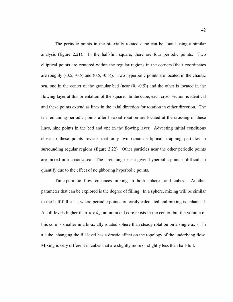
The periodic points in the bi-axially rotated cube can be found using a similar
analysis (figure 2.21). In the half-full square, there are four periodic points. Two
elliptical points are centered within the regular regions in the corners (their coordinates
are roughly (-0.5, -0.5) and (0.5, -0.5)). Two hyperbolic points are located in the chaotic
sea, one in the center of the granular bed (near (0, -0.5)) and the other is located in the
flowing layer at this orientation of the square. In the cube, each cross section is identical
and these points extend as lines in the axial direction for rotation in either direction. The
ten remaining periodic points after bi-axial rotation are located at the crossing of these
lines, nine points in the bed and one in the flowing layer. Advecting initial conditions
close to these points reveals that only two remain elliptical, trapping particles in
surrounding regular regions (figure 2.22). Other particles near the other periodic points
are mixed in a chaotic sea. The stretching near a given hyperbolic point is difficult to
quantify due to the effect of neighboring hyperbolic points.
Time-periodic flow enhances mixing in both spheres and cubes. Another
parameter that can be explored is the degree of filling. In a sphere, mixing will be similar
to the half-full case, where periodic points are easily calculated and mixing is enhanced.
At fill levels higher than 0δ>h , an unmixed core exists in the center, but the volume of
this core is smaller in a bi-axially rotated sphere than steady rotation on a single axis. In
a cube, changing the fill level has a drastic effect on the topology of the underlying flow.
Mixing is very different in cubes that are slightly more or slightly less than half-full.

43
Figure 2.21: Schematic diagram of periodic points in a bi-axially rotated cube. Four
periodic points exist in the cross section, two of which are elliptic centered within regular
regions. In the cube, this creates lines of periodic points associated with two orthogonal
directions of flow, shown on the right.

44
Figure 2.22: Regular regions in a bi-axially rotated cube. Top and side view show green
points trapped in regular regions and red points in the chaotic region (all but a few points
are removed to assist visualization of the regular regions). Analogous to the sphere,
regular regions exist along the zx −= plane in only two corners. The other periodic
points are located in a chaotic sea throughout the rest of the granular bed.

45
CHAPTER 3
COMPETITION BETWEEN MIXING AND SEGREGATION
IN 2D AND 3D CONTAINERS
This chapter discusses examples where transverse segregation and chaotic
advection co-exist. A quasi-two dimensional circular tumbler leads to
classic radial segregation, which is well understood. In a square,
segregation interplays with the underlying chaotic advection resulting in
dynamic equilibrium patterns. This interplay is also investigated in three-
dimensional systems such as bi-axially rotated spheres and cubes.
3.1 Modeling Inter-particle Interactions
3.1.1 Collisional Diffusion
Consider the model describing advection in a circular tumbler given by Eqns. 2.3-
2.5. The effect of collisional diffusion is incorporated in terms of the model developed
by Savage (1993). The collisional diffusion coefficient, Dcoll, is given by
( )dydvdqD x
coll2η= (3.1)
where dydv x / is the velocity gradient across the layer, and d is the particle diameter.
The prefactor ( )ηq , obtained by Savage via particle dynamics simulations, is a function

46
of the solids volume fraction, η ; in simulations, η is assumed to be a constant and
025.0=q is obtained by fitting to experimental data for mixing of identical particles in a
rotating cylinder. In terms of the model in section 2.2, the dimensionless form of
diffusion becomes
2
0
2
0
2
025.02
025.0δδdduDcoll == , (3.2)
where 12 0 =δu . Here, the dimensionless variables u, d , and 0δ are the average
velocity and the depth of the flowing layer at 0=x , respectively.
Collisional diffusion enters as a Langevin term in the particle advection equations.
Denote S as a white-noise term such that, upon integration over a time interval (Δt) it
gives a Gaussian random number with variance 2DcollΔt. The effects of diffusion may be
masked by convection. In our experiments the Péclet number along the layer, collDu / (a
measure of the relative importance of convection to diffusion) is approximately 102. The
Péclet number in the direction normal to the flow is factor 2
0δ smaller ( 1.003.0 0 << δ in
most cases). Thus, diffusion is important only in the y-direction.
The term S is added to vy (Eq. 2.4) such that
( ) ( )( ) ��
�
����
� −+=txthytuLv x
,12
δ, (3.3)
( )( ) ( )( ) S
txthytsxv y +��
�
����
� −−−=2
,δ, (3.4)

47
now making {vx, vy} a set of stochastic differential equations. The physical picture is as
follows: a passive blob advected in the flowing layer is deformed into a filament by the
shear flow and blurred by collisional diffusion until particles exit the layer (figure 3.1).
Diffusion enhances mixing by generating transport in the r-direction. This is the only
mechanism of transport across confining streamlines.
3.1.2 Segregation
Consider D-systems. The effects of segregation are incorporated in terms of drift
velocities with respect to the mean mass velocity (Khakhar et al. 1997b). Segregation,
like the effects of collisional diffusivity, is significant only in the direction normal to the
flow (apparent, again, when the Péclet number in each direction is considered). The
segregation velocity for the more dense particles (labeled 1) can be written as
( )( )d
Dv colls
yφργ −−−
=112
1 (3.5)
and for the less dense particles (labeled 2) as
( )
dD
v collsy
φργ −=
122 (3.6)
Here, sγ is the so-called dimensionless segregation velocity, ρ is the density ratio, d is
the particle diameter, and ( )tyx ,,φ is the number fraction of the more dense particles.
For elastic particles, sγ appears to be inversely proportional to the granular temperature;

48
Figure 3.1: Effect of diffusion on a passive blob. As the blob passes through the flowing
layer, diffusion blurs the edges of the blob, spreading across streamlines, thus enhancing
mixing.
Without diffusion With diffusion

49
however, for real particles a simple expression for sγ is not available, and it is treated as
a fitting parameter to match the rate of segregation. This model has been tested in
circular (nonchaotic) containers (Khakhar et al. 1999a). However, the main interest here
is how the final segregation pattern depends on container geometry and filling.
To add segregation into the advection model, assume first that the mean flow is
still the same as if all particles were identical, so that Eqs. 3.3 and 3.4 still apply. There
are two sets of advection equations; each corresponds to particle 1 or 2. The y-
component of the dynamical system representing the motion of the more dense particles
(labeled 1) is:
( ) ( )( )d
DS
hysx
dtdy colls φργ
δ−−
−+���
��� −
−−=112
2
11 , (3.7)
Whereas for the less dense particles (labeled 2), Eq. 3.7 becomes:
( ) ( )d
DS
hysx
dtdy colls φργ
δ−
++���
��� −
−−=12
2
22 , (3.8)
The two equations given above, combined with the corresponding equations for the x-
coordinates for each of the species, describe the evolution of the interpenetrating continua
from a Lagrangian viewpoint. Computations using this formulation are straightforward.
The number of particle trajectories simulated is roughly the same as the number of beads
in the corresponding experiment. Computation time increases by an order of magnitude
as compared to calculating Poincaré maps in chapter 2, computation time increases by an
order of magnitude. However, these calculations are significantly faster than discrete
element methods (DEM) for the same number of particles. Particles are labeled less or

50
more dense and are randomly distributed in the domain. They are advected according to
the equations of motion for each type of particle. The number fraction field, ( )tyx ,,φ , is
determined by defining a grid over the flowing layer and calculating the fraction of the
more dense particles in each bin of the grid.
The above model is a reasonable representation for the case of equal-sized
particles with different density. However, for mixtures of different-sized particles the
flow may be significantly affected by the composition of the layer. The local density
strongly depends on the local particle concentration. Consequently, the velocity field and
concentration field can be coupled with the proper volume fractions and size ratio of
particles. This issue is considered by Khakhar et al. 2001b. A model attempting to
capture this coupling alters the shape and thickness of the flowing layer based on local
concentration. As the authors point out, the resulting model is quite complicated.
This model (Eqns. 3.7 and 3.8) is also applied to 3D containers. Flow in three-
dimensional tumblers is also considered. The model represents flow in containers when
the flow only occurs in the transverse direction. The geometries of the tumblers and
symmetries of the protocol described in this chapter are chosen to ensure this. One
correction is necessary: a three-dimensional grid is defined over the flowing layer to
calculate the number fraction field (now ( )tzyx ,,,φ ). In the physical system, diffusion in
the z-direction is small. In a tumbler with consecutive rotations on two orthogonal axes,
diffusion in the z-direction is much smaller than the y-direction. Simulations with and
without a diffusive component in the z-direction result in roughly the same final pattern.

51
3.2 Experimental Details
3.2.1 Quasi-two Dimensional Experiments
Experiments in a quasi-two dimensional tumbler (figure 3.2) roughly approximate
a two-dimensional cross section of a three-dimensional tumbler. The analogy is only to
approximate since the packing density is greatly affected by the walls. The container in
this apparatus consists of a clear front-plate (Plexiglas), a center-plate made of either
foam core or aluminum, and an aluminum back-plate. The shape of the container is cut
into the center-plate, in this case either a circle or a square. The separation between the
front and back plates is only a few particle diameters (~6 mm). The center of the back-
plate is affixed to a long shaft that supports the weight of the tumbler and is grounded to
reduce static electricity on the beads. The container is rotated at a fixed angular velocity
using a computer controlled stepper motor (Compumotor) such that flow is in the rolling
regime (typically between 1 and 5 rpm). The actual value of the speed of rotation is not
significant; the mixing and segregation dynamics are roughly the same as rotation
produces flow that is continuous and produces a flat free surface (the so-called rolling
regime). As mentioned earlier, rotation rate only slightly affects the depth of the flowing
layer.
Two kinds of experiments are conducted:
(1) Evolution of a tagged blob – same particles, different colors
(2) Final shape of a phase boundary – particles of differing physical properties

52
Figure 3.2: Quasi-two dimensional apparatus. The container is a template of any shape
with a front and back plate. The front is Plexiglas and the back is aluminum that is
grounded to reduce static charge. The computer-controlled motor rotates the container at
a constant rate.

53
In the first case, experimental studies of blob deformation are carried out to
provide insight into the mixing process. Experiments using a mono-disperse material and
a tagged initial condition (material of a different color) are much more difficult than those
exhibiting segregation. Only experiments in half-full containers are considered. One
note of caution: the flowing layer expands. Therefore the container is filled slightly less
than half-full with spherical, noncohesive beads ( 2.0=d mm, Quackenbush). The goal
is to have the system precisely half-filled under dynamic conditions. A circular blob of
colored beads is positioned at the desired location in the bed. This is accomplished by
inserting a plastic template in the chaotic region, enclosing a circular region of beads.
Beads inside the template are replaced with tagged beads and the template is removed.
Great care is used to avoid agitating the material while positioning the blob, replacing the
front plate, and attaching the container to the motor. Digital photographs are taken at
different times to record the progress of mixing.
Quantitative comparisons between theory and experiment can be made in terms of
the intensity of segregation (Danckwerts 1952). The intensity of segregation, I, is
calculated as
( )2/1
1
2
1 ��
�
�
��
�
�
−
−= � =
NI
N
i mi φφ
, (3.9)
which is essentially the normalized standard deviation of the concentration of tracer
particles from the value for perfect mixing. The local concentration, iφ at the grid point
i, is measured at N uniformly distributed points within the granular bed and compared to

54
the average concentration, mφ . The location of the tagged particles is determined by
thresholding the image. The local concentration is calculated by measuring the area
coverage in each square of a template (in computations, iφ is the local number fraction
calculated using x, y-coordinates of each particle).
Experiments studying segregation are significantly easier to perform. D- and S-
systems are examined using a variety of noncohesive spherical beads with sizes ranging
from 0.8 to 2 mm and densities of 2.5 and 7.8 g/cm3 (glass and steel, respectively). In
this case, the tumbler is filled to various levels. All systems are initially well mixed.
More accurately, the tumbler is manually agitated until the resulting segregation pattern
has no apparent structure. Segregation experiments in each container for each fill-level
were repeated several times.
3.2.2 Three-dimensional Bi-axial Experiments
A sketch of the apparatus used for three-dimensional experiments is shown at the
top of figure 3.3. The apparatus is designed to perform a variety of protocols in different
tumblers. The same frame is used for all three-dimensional flow studies. The container
in the center, here shown as a sphere, is rotated by independent programmed motions in
two orthogonal directions (denoted as axis A and axis B). This is achieved by the
container first being secured into the apparatus on axis A. This is mounted into a rigid
platform that rotates about an orthogonal axis B. Adjustments on axis A allow the

55
Figure 3.3: Three-dimensional tumbler and rotation protocol. This apparatus allows
independent motion on two orthogonal axes. The rotation protocol shown at the bottom
produces alternating time-periodic flows on each axis. In this example, each axis rotates
β+�360 and then counter rotates β− so flow occurs for a full rotation and the free
surface is re-leveled at the beginning of each half cycle.
56
mounting of different size/shape containers (the maximum width allowed is ~ 18 cm) and
centering of the container. A stepper motor (Compumotor), mounted on the inner
platform produces rotation on axis A. This inner platform is mounted on and rotates
about axis B. Two uprights support axis B. A second stepper motor mounted on one of
the uprights drives the rotation of the inner platform. These two uprights are mounted on
a main platform that has legs that can be adjusted to level the entire apparatus.
Any amount of rotation on each axis prescribed in any order can be investigated.
For instance, if clockwise rotation of a specified duration on axis A and B is denoted U
and V respectively and counter clockwise rotation U’ and V’, one could produce any
consecutive repetition of rotations such as UV, UVVU, or even UVU’V’ which would
return any container to its original orientation. One can vary the amount of rotation on
each axis, producing even more complicated protocols (e.g U1V1V2U2U1’V1’V2’U2’,
where subscripts pertain to different amounts of rotation). Detailed analysis of the
symmetries of the rotation protocol is straightforward (Franjione and Ottino 1992). Even
the speed can be prescribed, but as mentioned in the quasi-two dimensional system, the
dynamics are not sensitive to rotation rate as long as the flow is within the rolling regime.
Furthermore, as will be described in chapter 5, simultaneous rotation of both axes is
possible.
While any set of rotations is possible, the motion of the container is physically
limited. This apparatus does not allow control of any arbitrary set of rotations of the
container. For instance, the angle of axis A to horizontal depends on the amount of
rotation on axis B. Considering this, logical decisions regarding rotation protocol are

57
necessary to produce a desired flow. Flow does not start until the free surface reaches the
angle of critical stability ( iβ ), and the flow remains at the angle of repose β after rotation
ends (the difference between these two angles for the spherical beads used in these
studies typically �10<− ββ i ). Also, it is obvious that when axis B is near vertical no
flow results from rotation on axis A.
Figure 3.3 also shows an example of a rotation protocol designed to produce the
bi-axial flow protocol as will be modeled in section 3.3. Motions on each axis are
discrete, where the flow is fully developed after just a few degrees after start up (roughly
ββ −i ) and flow comes to rest quickly after stopping. To directly compare the results of
the experiment to the simple model, both the container and the free surface should start
level. This protocol, using above terminology, is U1U2’V1V2’. Rotation U1 is β+�360 ,
where flow occurs for approximately 360º of rotation from iβ until β+�360 . U2’ is
counter clockwise rotation of β− . This returns the container and free surface to level
(without flow) before starting rotations on the orthogonal axis, V1 and V2’.
Visualization of the segregation pattern resulting from different flows is difficult
in three-dimensional systems. Until recently, the only method was to sample material by
the use of thieves – long tubes used to extract particles from the middle of the bed.
However, this technique is invasive – disturbing the final state of the granular bed – and
it is shown to poorly represent concentrations throughout the system (Wightman et al.
1996). Another invasive technique is to solidify and slice the granular bed to reveal the
internal structure. This is accomplished by pouring liquid agar into the bed and allowing

58
it to cool. This technique has been shown to be rather successful (but difficult and time
consuming). Scanning the granular bed using NMR is a rather successful non-invasive
way to visualize the interior. However, results using NMR are limited by speed and
precision (especially in rapid flows), but have been used successfully by Nakagawa et al.
1993 to characterize granular flow and by Nakagawa et al. 1997 to study radially
segregated structures. This technique is only possible in some systems. Bead choice is
critical; for instance, glass beads are invisible. Also, the apparatus cannot have any metal
parts near the magnet. Accessibility to this equipment is limited.
Another possibility, but one that changes the physics of the system, is to run
experiments under slurry conditions. Jain et al. 2001 performed experiments
investigating axial segregation – producing alternating bands of different types of
particles along the axis of rotation – under slurry conditions. Using a liquid brings
substantial benefits. Using a suitable fluid (for instance, ~66% NaI solution) that roughly
matches the refractive index of the larger/lighter clear beads making them translucent.
This same methodology is used in experiments described in this chapter using 0.2 mm
black and 0.8 mm clear glass beads.
In dry systems, index matching is not possible. However, we use a technique that
works reasonably well using large clear beads (2.0 mm glass) and small fluorescent beads
(0.8 mm glass). Using UV light, the fluorescent beads glow brightly and the beads
closest to the container walls become visible (fluorescent beads within ~ 10 particle
diameters from the boundary). In experiments described here, the size of the sphere is R
= 70 mm for the dry systems, R = 40 mm for the slurry experiments. The cube used for

59
dry experiments is 100 mm and 60 mm on a side for slurry conditions. The smaller
containers are used in slurry experiments to minimize the overall weight of the container,
beads, and fluid.
3.3 Mixing and Segregation in a Quasi-Two Dimensional Tumbler
3.3.1 Chaotic Mixing with Diffusion
Consider half-full two-dimensional tumblers. Figure 3.4 shows computations and
experiments conducted in the circle and square. The initial condition is inset in the top
left corner of each picture – in the square, the blob is placed in the chaotic region. After
one pass through the flowing layer, the blob of darker particles is spread into a wedge. In
a circle, diffusion appears to mix better than stretching of the underlying flow – the blob
is mostly blurred across closed streamlines.
A comparison between theory and experiment is shown in figure 3.5 for blob
deformation in a square. There is good qualitative agreement between the two.
Comparison to the Poincaré map shows that several features of the underlying flow
structure are apparent even when diffusion is included: blobs are stretched along unstable
manifolds, and the density of particles in the regular regions is small. This is analogous
to passive dyes aligning with unstable manifolds of the flow as observed in the mixing of
fluids (Swanson and Ottino 1990). A quantitative comparison between theory and
experiment is shown in figure 3.6. There is again good agreement between the two for
the variation of intensity of segregation with time. Note that there are no adjustable

60
Figure 3.4: Blob experiments and computations. All particles are the same (0.2 mm
glass spheres) except for color. After just two rotations, diffusion spreads the initial
condition (upper left corner of experimental pictures) into a wedge.
Experiment Computation

61
Figure 3.5: Mixing of tracer particles in a square. This is a comparison of an experiment
using colored glass beads (left) and a simulation using the model (right). The number of
rotations for each image is listed in the lower right corner.

62
Figure 3.6: Variation of the intensity of segregation as a function of rotation
corresponding to the experimental and theoretical results in figure 3.5. The filled circles
represent experimental values and the open circles denote values obtained from the
model. Error bars result from uncertainties in image processing.

63
– the depth of the flowing layer, 0δ , is measured in the experiment using streakline
images.
While diffusion blurs the invariant structures of the underlying flow in laboratory
scale tumblers, in larger systems this is not so. Since the depth of the layer 0δ is
proportional to the flow distance L, the Péclet number scales as 2)/(~ dLPe . Therefore,
increasing the size of the tumbler decreases the rate of collisional diffusion. This can be
illustrated by means of computations comparing mixing in the square and circle, for large
and small sized containers. Figures 3.7 and 3.8 show the variation of the intensity of
segregation as a function of time for four different mixers and two different initial
conditions. In figure 3.7, the initial distribution corresponds to one material layered on
top of the other with colored particles on the bottom; the other initial distribution (figure
3.8) corresponds to the left-half of the bed containing colored particles and the right-half
of the bed white particles. In practice, the top-bottom placement is more practical. The
intensity of segregation for all cases is initially 5.0=I , which corresponds to the
theoretical value for a completely segregated mixture containing 50% of the colored
particles. In each figure, the distribution of particles in a large circle and square are
shown after 20 rotations.
The decay in intensity of segregation with time for the different tumblers and
initial conditions is different. In the case of the circular mixer, increase in the mixer size
results in a significant reduction in the rate of mixing. This is also the case in the square
mixer. However, comparing at equal sizes (i.e., equal Péclet numbers) we see that the

64
Figure 3.7: Variation of the intensity of segregation vs. mixer rotation obtained for
mixers of different shapes and sizes predicted by computations. The initial condition is
initially unmixed top-bottom. The large systems correspond to a Péclet number 410=LPe , and the small systems to 210=SPe , which indicates a mixer size ratio of 10.
The final distributions of particles in the large tumblers after 20 rotations are shown at the
bottom.

65
Figure 3.8: Variation of the intensity of segregation vs. mixer rotation obtained for
mixers of different shapes and sizes predicted by computations. The difference between
this and results in figure 3.7 is the initial condition (left-right here). Clearly the initial
distribution has an effect on mixing in the square. At the bottom, after 20 rotations the
distribution of particles in the large square shows black and white particles trapped in the
two separate regular regions.

66
square container mixes faster than the circular one for both the sizes considered here.
Furthermore when compared at equal sizes (i.e., equal Péclet numbers) it is apparent that
the square container mixes faster than the circle. These results indicate that chaotic
advection becomes more important with increasing mixer size. Chaotic mixing is thus
essential for practical applications, given that large mixers are the norm in industrial
processes.
One could argue, however, that a good tumbler design should mix well regardless
of the initial condition. Mixing in a large square is clearly biased by the initial
distribution. Material within the regular regions mix isolated from the rest of the flow.
Therefore, mixing is better when the regular regions contain both black and white
particles, as is the case in the top-bottom orientation. This is clear in the picture at the
bottom of figure 3.7. In the left-right initial condition, each regular region only has one
type of particle initially isolated from both the chaotic regions and the other type of
particle. In fact, looking closely at the graph in figure 3.8, mixing in both a circle and
square is initially very similar (as seen in figure 3.4). Only after a given number of
rotations is it clear that the material in the square container mixes faster. In the large
container it is clear that there is little mixing between black and white particles in the
regular regions, even after 20 rotations. In fact, although mixing is occurring, the square
looks similar to the initial condition where most black particles are on the left side.

67
3.3.2 Competition Between Segregation and Chaotic Advection
Consider the same systems as above but now with a bi-disperse granular mixture
(as considered in Hill et al. 1999a,b). Under flow bi-disperse granular materials
segregate. The focus here is on the final segregation pattern without regard to dynamics
that may depend on the initial conditions. The easiest case to understand is the circle.
The classic radially segregated structure is shown on the left in figure 3.9. In this case,
the dynamics in the flowing layer cause the smaller (more dense) particles to move down
in the layer. These particles have a low probability of reaching the end of the layer,
leading to a segregated core –segregation is complete after just 1 or 2 revolutions. The
model clearly captures this behavior. The closed streamlines represented by the Poincaré
map are shown below these segregation patterns and the boundary between the two
“phases” lies along the streamlines.
The case of the square is more complicated. First consider the half-full square.
Materials begin segregating radially in 1 or 2 revolutions. After this, smaller/denser
material moves toward the corners, deforming the interface between the two phases and
forming two lobes. Comparing the pattern in the experiment and predicted by the
computations to the Poincaré map, the segregated core clearly tags the regular regions of
the flow. This is significant and explained in more detail below. The two lobes are not
symmetric to reflections across 0=x , however they are rotationally symmetric (the
pattern seems to “pinwheel” clockwise). The Poincaré map appears symmetric across

68
Figure 3.9: Segregation in half-full circle and square - from top to bottom, experimental
D-system, experimental S-system, computation, and Poincaré map. The phase boundary
roughly conforms to the close streamlines (circle) or the regular regions (square).

69
0=x . However, there is a hyperbolic point at (0, -0.5) near which the underlying flow is
asymmetric across 0=x . Its unstable manifolds initially follow along the vectors (-1, 1)
and (1, -1), pulling material away from the hyperbolic point. The phase boundary
between the two materials seems to roughly follow along a heteroclinic orbit around the
regular region into the other hyperbolic point (located in the flowing layer).
As shown in chapter 2, the underlying advection patterns are very sensitive to the
degree of filling. Likewise, the segregation patterns are also sensitive to filling (figure
3.10). Parallel S-system and D-system experiments, computations, and Poincaré maps
are shown for 25%, 45%, 50%, 55%, and 75% full squares. Clearly the Poincaré map
predicts the shape of segregation (with the exception of the 55% full S-system). In the
Poincaré maps for the 45% and the 55% cases, the KAM surfaces inhibit mixing in the
radial direction. In the D-system and computations, the phase boundary is roughly traces
these KAM surfaces. The stripes formed in the 55% full S-system clearly show another
process at work. In S-systems at this filling, the layer may alternate between nearly
100% small particles and 100% large particles. Thus, depending on the composition of
the layer, the flow may become time-periodic under steady rotation. Khakhar et al.
(2001b) demonstrates that this also happens in a circle with the correct filling and
material parameters. A model describing this phenomenon alters the shape of a
piecewise linear flowing layer based on the local concentration. This is a clear example
of sensitivity to material properties.

70
Figure 3.10: Segregation patterns in a square with different fillings. From left to right –
experimental results in a D-system and S-system, Poincaré map, and computation. The
model captures the behavior except for the 55% full S-system where the layer velocities
are coupled to the concentration. In all other cases, the topology of the underlying flow
may assist in predicting the shape of segregation.
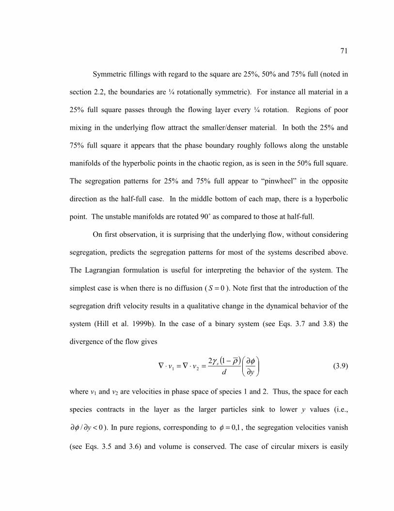
71
Symmetric fillings with regard to the square are 25%, 50% and 75% full (noted in
section 2.2, the boundaries are ¼ rotationally symmetric). For instance all material in a
25% full square passes through the flowing layer every ¼ rotation. Regions of poor
mixing in the underlying flow attract the smaller/denser material. In both the 25% and
75% full square it appears that the phase boundary roughly follows along the unstable
manifolds of the hyperbolic points in the chaotic region, as is seen in the 50% full square.
The segregation patterns for 25% and 75% full appear to “pinwheel” in the opposite
direction as the half-full case. In the middle bottom of each map, there is a hyperbolic
point. The unstable manifolds are rotated 90� as compared to those at half-full.
On first observation, it is surprising that the underlying flow, without considering
segregation, predicts the segregation patterns for most of the systems described above.
The Lagrangian formulation is useful for interpreting the behavior of the system. The
simplest case is when there is no diffusion ( 0=S ). Note first that the introduction of the
segregation drift velocity results in a qualitative change in the dynamical behavior of the
system (Hill et al. 1999b). In the case of a binary system (see Eqs. 3.7 and 3.8) the
divergence of the flow gives
( )
���
����
�∂∂−
=⋅∇=⋅∇yd
vv s φργ 1221 (3.9)
where v1 and v2 are velocities in phase space of species 1 and 2. Thus, the space for each
species contracts in the layer as the larger particles sink to lower y values (i.e.,
0/ <∂∂ yφ ). In pure regions, corresponding to 1,0=φ , the segregation velocities vanish
(see Eqs. 3.5 and 3.6) and volume is conserved. The case of circular mixers is easily

72
visualized. The denser particles sink to lower positions in the layer while lighter particles
rise, which translates into a radial motion with the denser particles moving to the central
core and the less dense moving to the periphery. At equilibrium there is complete
segregation with all of the denser particles occupying the central core and all of the
lighter particles in the periphery, with the boundary between the two being given by the
streamline bounding an area fraction equal to the volume fraction of the denser beads. In
noncircular mixers there is also an initial tendency for the denser particles to initially
move to form a central core and for the lighter particles to migrate to the periphery.
However, in this case streamlines are not invariant curves, and thus the core is distorted
and mixed because of advection.
The key to the structure formation lies in the invariant curves of the mapping. An
invariant curve composed entirely of one of the species is preserved by the mapping
(which now coincides with that for a single component because the segregation velocity
vanishes). Thus, the structure formed is determined by the surviving KAM curves of the
Poincaré section for the single-component system. The region within the outermost
KAM curve enveloped by the core formed by the dense particles is invariant as is the
peripheral pure region of light particles outside the innermost KAM curve. The effect of
diffusion primarily blurs the structures. When the core size exceeds that of the invariant
region, chaotic advection and diffusion act in concert to mix the particles outside the
invariant region (Hill et al. 1999b).
This analysis, as described by Hill et al. (1999b), is relatively successful in
explaining the phenomena seen in two-dimensional tumblers. In fact, Hill et al. (1999b)

73
reports that if three different sizes of beads are tumbled, with only a small amount of the
middle size, the middle sized beads reside near the phase boundary that is seen with only
two materials (they use this technique only to make the phase boundary more clear).
Beads of multiple sizes segregating and producing flow in the rolling regime could
possibly give “experimental contour plots” of the underlying flow. One also might ask to
what extent do these results apply to the full three-dimensional case. This is considered
in the next section where chaotic advection in bi-axially rotated containers interacts with
segregation.
3.4 Segregation in a Sphere and Cube: Bi-Axial Rotation
Consider now the interplay of chaotic advection and segregation in three-
dimensional granular systems. In a cylindrical tumbler rotating on its primary axis, the
flow is essentially two-dimensional with most flow occurring in the cross section.
Because of this, the dynamics in the transverse direction are similar to that of a 2D flow.
First, smaller/denser particles segregate to the middle of the granular bed – classic radial
segregation is seen in containers that have a circular cross section, and lobe formation is
seen in containers with a square cross section. This is evident in a half-full cube (figure
3.11) – after just a few rotations (the bottom of the cube rotates from left to right) the two
lobes of the segregated core are seen from the bottom as two horizontal lines. From this
perspective, smaller beads are glowing from behind the larger clear beads. Already it is
clear that there are some slight end effects preventing the lobes from extending, as seen
here, completely from the top of the picture to the bottom. After many rotations, these

74
Figure 3.11: Bottom view of a cube after 6 and 50 rotations (rotation moves image from
left to right). Two lobes form as seen in the two-dimensional segregation. They
eventually contract along the axis of rotation to roughly form a band. The beads are
brighter in the bottom picture as they reach toward the boundaries of the cube.
Axis of
Rotation
6 rotations
50 rotations

75
Figure 3.12: Bottom view of a long tumbler with square cross section (Hill et al. 1999b).
Even in the presence of axial segregation, chaotic advection clearly plays a role in the
two-dimensional cross section.
Axis of
Rotation
Axis of
Rotation

76
lobes contract toward the middle due to segregation along the axis of rotation. In an
elongated tumbler, multiple bands form after many rotations, but this underlying
segregated structure is still apparent (figure 3.12 from Hill et al. 1999b). The
combination of axial banding and underlying chaotic advection is discussed in more
detail in chapter 5.
The bi-axial protocol is designed to generate a simple example of a chaotic three-
dimensional flow. The aim is also to eliminate axial banding in order to study how
segregation in the transverse plane interacts with three-dimensional flow. Consecutive
rotations on orthogonal axes produce flow in one direction that is intended to cancel the
effects of axial segregation formed by flow in the previous direction – this may or may
not be the case, but axial bands do not exist. The location of periodic points of this flow
are given analytically in chapter 2 – there are both regular regions and chaos in both the
sphere and the cube. In the sphere, the periodic points are located in the '' zx =
(hyperbolic) and the '' zx −= (elliptic) planes at ( ) 221¼ xzy −−≅ . Two regular
regions exist in the '' zx −= corners. Hyperbolic points scattered throughout the bed
enhance mixing, the strongest of which is located in the center of the granular bed
(mixing near this point enhanced relative to flow in each direction).
The primary difference between these two geometries is that flow in a cube is
chaotic at any instant, whereas in the sphere, it is the time periodicity of the protocol that
generates chaos. As described above, the underlying flow has a large effect on the shape
of the phase boundary between the segregated regions in two-dimensional flows. It is

77
unclear if this same behavior will exist in three dimensions. If so, smaller/denser beads
will be pulled towards the regular regions such that the segregation will form
“experimental” Poincaré maps. This is computationally investigated in a half-full sphere
and cube.
Consider a bi-disperse system in a bi-axially rotated sphere. Computations using
the model given by Eqs. 3.3, 3.7 and 3.8 show that the denser material migrates to the
center after just one or two cycles. Segregation is almost purely radial (figure 3.13 – red
particles are more dense, green are less dense). No mechanism driving axial segregation
is built into the model. There is little evidence that the segregation is affected by the
underlying chaotic advection. Slices in the x-y and z-y planes at z or 5.0,0,5.0−=x
respectively show that each slice looks roughly the same as segregation seen in a circle.
Denser material does not appear to favor the regular regions of the flow, nor does it avoid
the regions of chaos. Different volume ratios of beads exhibit the same pattern.
Two different types of experiments are used to further investigate these results.
First, large clear beads and small fluorescent beads (2.0mm and 0.8mm respectively) are
tumbled bi-axially in the sphere. Under UV light, the smaller beads all seem to reside in
the center (figure 3.14). After as many as 30 cycles, this pattern remains the same. There
are no details captured from this bottom view picture that indicate anything but almost
purely radial segregation (as predicted by the model). To check that this non-invasive
technique is accurate, another experiment is performed under the same conditions using
larger red and smaller blue beads and solidified with agar after 30 cycles. A center cut in

78
Figure 3.13: Computation of segregation in a bi-axially rotated sphere. Segregation
appears to occur mostly in the radial direction. Slices are in the x’y’ and z’y’ planes at –
0.5, 0.0 and 0.5 along the orthogonal axis.

79
Figure 3.14: Experiments in bi-axially rotated sphere. Top picture is the bottom view of
the sphere partially full with fluorescing smaller beads. In order to verify that the
segregation is mostly radial, the granular bed is solidified with agar and sliced. The slice
is in the x’y’ plane at 0' =z .

80
the x-y plane along 0' =z reveals roughly the same pattern. The smaller blue beads form
an almost purely radially segregated core.
There is good qualitative agreement between the experiment and computations.
Both predict radial segregation. It is somewhat surprising that the underlying chaotic
advection seems to have little effect on the segregation pattern. This fact can be
explained by taking a closer look at the Poincaré map of this flow (figure 2.20). The
volume of the regular regions is small. Also, the points trapped in the regular region
appear as if they are all located roughly at the same radius. If regular regions “attract”
smaller beads, they could do so without distorting the phase boundary in the radial
direction. In the same way, the hyperbolic points in this flow have unstable manifolds
that seem to point orthogonal to the radial direction. If the phase boundary follows along
the unstable manifolds, as it does in the two dimensional experiments, there would be no
evidence of distortion in the radial direction. Aside from this, it is also surprising that
segregation is mostly radial considering that flow in S-systems can be more complicated
than represented by this simple model (as seen in the 55% full square in figure 3.10).
The bi-axially rotated cube presents even more intriguing behavior. Prior to
performing computations, imagine two scenarios (figure 3.15). One scenario assumes
that the regular regions of the three-dimensional map will attract the smaller/denser
material. This would result in two lobes forming two spots covering the regular regions
in the Poincaré map. The other scenario assumes that dynamics in the two-dimensional
flow are dominant such that invariant structures formed by three-dimensional flow

81
Figure 3.15: Depiction of possible outcomes. The final segregation pattern may
resemble picture A at the end of each rocking cycle if regular regions in the three-
dimensional flow captures smaller/denser particles analogous to the two-dimensional
system (the regular regions are shown to the right of A from figure 2.22). However, if
lobe formation is only an artifact of two-dimensional flow, the picture may have either
four lobes (B) or two elongated lobes (C) at the end of each cycle (like those shown to the
right of C from figure 3.10).

82
(different than those in two-dimensions) have little consequence on the shape of the
phase boundary.
The result of this could be four lobes, one in each corner (the regions where
regular regions exist for flow in both directions). Moreover, the biaxial protocol could
simply produce a time-periodic pattern, where elongated lobes form from flow in each
direction associated with the direction of flow in each half of the cycle.
In computations, a three-lobed segregation pattern that forms after 6 cycles (figure
3.16) does not correspond to either of the above scenarios considered in figure 3.15.
Computations in a bi-axially rotated cube show that red (more dense) particles form
segregated lobes. This is clear in vertical slices (figure 3.16, left), as was done in the
sphere (figure 3.13), but the lobes are easier to see when the bottommost particles
(particles below 7.0−=y ) are removed (figure 3.16, right). Three lobes are formed, all
of which avoid the center of the cube. Two of these lobes, those located in the upper and
lower right corners, are very clear. The other lobe on the left side resembles one of the
two elongated lobes formed when rotating on a single axis (figure 3.11) but less coherent.
Clearly this is unlike the radial segregation seen in the sphere – the shape of the
associated three-dimensional phase boundary is complicated.
While this computational result is quite surprising, it correctly predicts the
segregation pattern seen in experiments (figure 3.17). In dry experiments, the three-lobe
structure that arises after just a few cycles is very clear when using fluorescent particles
and UV light. The lobes avoid the center of the granular bed, two in the upper and lower

83
Figure 3.16: Computations after 6 cycles of bi-axial rotation in a cube (left – vertical
slices, right – horizontal slice). The segregation pattern avoids the center and migrates
into three different lobes of denser (red) material. In the “bottom view”, the bottommost
material is removed to show an interior slice at y = -0.7

84
Figure 3.17: Comparison of an S-system, D-system and computations of pattern
formation in a bi-axially rotated cube. Similarities between the different experiments are
remarkable. This complex pattern is captured by the model.

85
right corners and the third on the left side. This pattern is very reproducible and stable
for at least 30 cycles. In fact, this pattern is seen twice in each rocking cycle. This
picture shows the pattern at the end of the rocking cycle. Because of the symmetry of the
protocol (flow could start in either direction), this pattern appears again, rotated 90�
counter-clockwise half way through the cycle.
The experiment and computation are in good qualitative agreement. The relative
locations, sizes and shapes of the lobes in the experiments are roughly matched by the
computations. This is surprising in light of the following:
a) The model essentially only considers dynamics in the transverse direction.
b) Computations are of a D-system (simple), whereas the experiments are an S-
system (complicated – flow may couple with local concentration).
Consider now a similar, perhaps more complicated experiment run under slurry
conditions. The interstitial fluid properties are not considered as if the particles are in a
vacuum. Air likely has a slight effect on the flow, but replacing air with a more viscous
fluid makes this system even more complicated. Lubrication forces between particles in
the flowing layer change the depth of the flowing layer and the rate of segregation (Jain
et al. 2002). For this reason, it is remarkable that the same three-lobe pattern forms in a
bi-axially rotated cube under slurry conditions (figure 3.17 also shows the dry case and
computations and the Poincaré map predicting this pattern). Substituting air with a NaI
solution allows index matching of the larger glass beads, making the smaller black beads
visible. Furthermore, this system is in a smaller cube with different sized beads (0.2 mm
and 0.8 mm). Comparing the resolution of each of the two experimental pictures

86
suggests that the new technique using fluorescent beads and UV lighting in the dry
condition may reveal the internal structure as well, if not better than index matching. The
relative brightness of fluorescent beads gives depth to the contours of the internal
segregated structure.
Comparing these experiments and the computation, it is clear that the material
parameters appear to have little influence on the final segregation patterns in almost all of
the two and three-dimensional systems considered in this chapter. In these systems, the
shape of segregation seems to follow along with the invariant structures of the underlying
flow. If this is universally true, evaluating the shape of the phase boundaries of
segregated patterns could be used as a tool that suggests the underlying flow. As
mentioned in the quasi-two dimensional system, mixtures of three or more different sizes
of beads segregate so that the middle phase resides between the small and large sized
beads. Multiple phase boundaries would show more of the underlying flow behavior in a
single experiment.

87
CHAPTER 4
KIMEMATICS OF A ROTATING-ROCKING SPHERE
This chapter considers chaotic advection within a rocking-rotating sphere.
Modeling is straightforward, but the underlying dynamics are not; for a
fixed amplitude, small changes in rocking frequencies give rise to
radically different segregated structures. The topology of the underlying
flow has implications on the stability of segregation in the experimental
system.
4.1 Model
Consider a half-full sphere. The sphere rotates on one main or primary axis
denoted A which in turn is moved in a prescribed manner about the axis labeled B (figure
4.1). The rotation on axis A induces a flow that mixes primarily in the x-y plane.
Rocking the main axis of rotation induces flow in the axial direction z. Conventional
thinking indicates that adding axial flow should enhance mixing beyond diffusion-limited
axial transport, as occurs in three-dimensional tumblers rotated on a single axis.
Moreover, time-periodic flow induces chaos, which also enhances mixing.
The spherical geometry allows modeling as follows. The amount of rotation
around axis A is denoted θ . The angle of axis A to the horizontal is ( )θγ fAsin= .

88
Figure 4.1: Rocking protocol and coordinates. In this protocol, the sphere has constant
rotation on axis A and rocking motion on axis B. Note that the flow is in the x-direction
at an angle β to x’-direction relative to the lab.

89
Thus, for a frequency 1=f , one rocking cycle occurs every full revolution on axis A.
f/2πθ = corresponds to one cycle. The instantaneous angular velocity about axis B is
( )θθγ fAfdd cos/ = .
The free surface is assumed flat – therefore it is always circular. Coordinates
associated with this model are as follows.
• The flowing layer frame (x, y, z) – chosen such that the x-axis always
points in the flow direction, the y-axis points opposite gravity, and the
z-axis is orthogonal to the xy plane.
• The laboratory frame (x’, y’, z’) – chosen such that the x’-axis points
along axis B, y’-axis points opposite gravity, and the z’-axis is
orthogonal to the x’y’ plane.
The origin for both of these coordinate systems is stationary at the center of the circle that
is also the center of the sphere. The instantaneous angle between x and x’ is denoted as
β .
Assume that within the flowing layer each cross section in the flow direction is
independent of its neighbors. Moreover, assume that the flow readjusts instantaneously
to changes in orientation of the sphere. Surface velocities at the air-granular bed
interface scale with the local free surface half-length 21 zL −= (figure 4.2). The
flowing layer is comprised of a thin lens-like region of form ( )( )2
0 /1 LxL −= δδ - the
same as described in section 2.2.

90
The flow direction relative to lab coordinates is given by β . This angle is
determined by the ratio of angular velocity about axis B and axis A, where
( ) ���
����
�=
γθ
cos
/tan 1- dd��
. (4.1)
Rocking amplitudes of �90≥A are not considered, therefore �� 9090 <<− β for all f.
The equations for velocity in the flowing layer are
���
��� +=
δyuLMvx 12 (4.2)
2
���
���−=
δyMxvy . (4.3)
The function M in (Eq. 4.2) and (Eq. 4.3) is given by
( )2
2cos ���
���+=
θγγ
ddM . (4.4)
Particle path-lines are calculated by integrating the above equations in the flowing layer
with solid body rotation in the bed. A pictorial representation of the relationship of
rocking angle and direction of flow is depicted in figure 4.3. The flow only points in the
x’ direction when 0/ =θγ dd . This model applies to any prescribed motion about axis
B. Consider sinusoidal rocking as a perturbation to a base case where axis A is always
horizontal and each cross section is a simple circle (as described in section 3.1). When A
and f are non-zero, flow occurs in the axial direction. Large values of A and f produce
flow that is almost perpendicular to the x’-direction. The goal is to investigate the
behavior of the system in the A-f phase space.

91
Figure 4.2: Surface velocities at the midsection of the free surface. Velocity scales with
the length of the free surface 21 zL −= . The y-axis points out of the page.

92
Figure 4.3: Relationship between rocking angle and instantaneous flow direction.

93
4.2 Quasi-periodic and Chaotic Path-lines
Consider now the flow generated within the sphere. A few general observations
are in order. In general, most streamlines produced by solid body rotation intersect the
flowing layer. However, a cone-shaped stream-surface exists where material within it
circulates without intersecting the surface flow. This region is illustrated for a rotating
sphere that is rotated at a constant angle of inclination in figure 4.4 – without rocking
streamlines close onto themselves. The size of this region depends on the value of γ ,
and all streamlines intersect the flowing layer when 0=γ . This cone is analogous to the
core in the center of a more than half-full tumbler. With rocking, this cone-shaped core
grows and shrinks periodically. Following a path-line (figure 4.5) shows that some
particles are temporarily trapped within this region. These trajectories occasionally get a
“kick”, temporarily rotating without entering the flowing layer. This happens to most of
the particles that are located near the projection of axis A throughout the granular bed.
Other initial conditions give rise to quasi-periodic trajectories (figure 4.6). These quasi-
periodic trajectories may be confined to a small region or spread seemingly throughout
the sphere. In either case, mixing is poor.
In the lab frame (x’, y’, z’), particles flow on hemispherical surfaces when rotating
as a solid body in the bed. Consider tracking the radial position of a particle with a quasi-
periodic trajectory. After passing through the flowing layer, it returns close to the same
hemispherical surface when exiting the flowing layer (figure 4.7 - r is calculated each
time the trajectory leaves the flowing layer). The figure shows the dynamics after ~200

94
Figure 4.4: Sphere rotating on angle. Without rocking, flow produces closed
streamlines. Flow in the cone-shaped region does not intersect the flowing layer.

95
Figure 4.5: Typical chaotic path-line. Occasionally, this trajectory is temporarily trapped
in the cone-shaped region depicted in figure 4.4.
Top
Front
Side

96
Figure 4.6: Typical quasi-periodic path-line. Although the particle explores much of the
container in the axial direction (top picture), mixing is poor in the region neighboring this
particle at any instant.
Top
Front
Side

97
rotations. It is clear that the distance traveled in the r-direction is small and the behavior
is nearly periodic. In this graph, the aggregate numerical error during these 200 rotations
is comparable to the width of the line plotted. On the other hand, a chaotic trajectory also
moves slightly in the r-direction undergoing small, seemingly random, jumps. Mixing in
the chaotic regions is very poor in the radial direction. All of these trajectories, chaotic or
quasi-periodic, are trapped within a small range of r over many rotations of the tumbler,
effectively flowing on a quasi-two dimensional hemispherical surface.
4.3 Poincaré Maps
Poincaré maps are computed by plotting the particle position at the end of each
rocking cycle. In these computations, locations are plotted for 200 cycles. By definition,
Poincaré plots yield more information about the long-time dynamics than path-lines.
Because all particles roughly return to the same surface, the initial conditions for each
plot have the same initial radial position. Most of the maps described in this chapter have
initial conditions starting at 95.0=r , giving information only about the dynamics near
the container walls. However, even though this technique is limited, this method will
allow comparison between the model and experiments. Most experiments (unlike those
mentioned in section 3.2) reveal only what is in immediate contact with the containers’
walls.

98
Figure 4.7: Time evolution of the radius of a quasi-periodic trajectory (black) and a
chaotic trajectory (red). The radius is calculated each time the particle leaves the flowing
layer over ~200 rotations. The quasi-periodic trajectory has small periodic motion in the
r-direction. The chaotic trajectory is irregular, but also has relatively small radial motion.
This suggests that most dynamics occur within hemispherical “shells” with little radial
transport.

99
As the frequency is decreased, the tumbler rotates multiple times in each rocking
cycle. As 0→f , each computation takes an excessively long time. Therefore, most
computations are limited to the range 5.15.0 << f . Many Poincaré plots were computed
within this range in order to extract the most important aspects in the flow. These maps
are organized in Appendix A with only a few highlighted in this chapter.
Figure 4.8 shows a sample of the various dynamics observed. View is from the
bottom, where the main direction of rotation moves material from top to bottom – and
rocking is side to side (i.e. left to right and right to left). Quasi-periodic trajectories are
closed orbits; chaotic regions appear as a seemingly random scatter of particles. All of
these maps are 180º rotationally symmetric. This symmetry is exploited to reduce
computational time by only calculating half of the particle paths represented by each
map. Most maps at low amplitudes or low frequencies look similar to figure 4.8a
(�30=A , 925.0=f ), where almost all trajectories are quasi-periodic and chaotic regions
are small, located near the ends of the sphere, almost out of view.
The map in figure 4.8b (�5.42=A , 6.0=f ) shows that large regular regions
where particles circulate about a periodic point can form. Higher order periodic points
exist at different frequencies forming chains of islands (figure 4.8c, �5.47=A , 65.0=f ).
Some periodic points are hyperbolic (figure 4.8d, �60=A , 95.0=f ), where stretching is
enhanced only locally. In this figure, all trajectories shown appear to be chaotic. At
higher values of f, regular regions are smaller or non-existent (figure 4.8e,
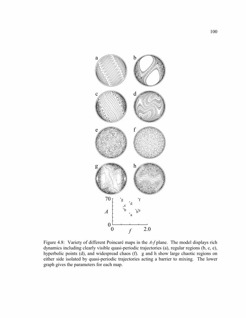
100
Figure 4.8: Variety of different Poincaré maps in the A-f plane. The model displays rich
dynamics including clearly visible quasi-periodic trajectories (a), regular regions (b, c, e),
hyperbolic points (d), and widespread chaos (f). g and h show large chaotic regions on
either side isolated by quasi-periodic trajectories acting a barrier to mixing. The lower
graph gives the parameters for each map.

101
�40=A , 475.1=f ), and at the highest values of amplitude and frequency computed,
apparently all trajectories are chaotic (figure 4.8f, �70=A , 475.1=f ). In this case, there
may be periodic points with regular regions that are not resolved. Figures 4.8g,
h(�70=A , 5.0=f and
�40=A , 325.1=f respectively) show that these chaotic regions
may reach near the center, but as long as quasi-periodic trajectories exist, there is no
transport from one hemisphere to the other.
Concentric Poincaré maps shown in figure 4.9 - the interior revealed as if peeling
an onion - represent the dynamics at each radial position (�45=A , 6.0=f ,
9358.03258.0 << r ). For ease of comparison, each map is plotted with same average
density of points – less initial conditions in the innermost maps. The relative size of the
chaotic regions compared to the “surface” shown is relatively the same at each radial
position. However, it seems that structures existing near the boundaries (near 1=r )
move from right to left, then shrink and disappear as 0→r . In fact, the way the maps
transform as r decreases is similar to the way the maps transform with decreasing
frequency. This will become clearer in the next section where the sensitivity of regular
regions to both f and A is investigated.
4.4 Flow Bifurcations
Consider the regular regions that are shown in figure 4.8b. The existence of the
periodic points at the center of these regular regions is sensitive to f. The way in which
these regular regions that appear at a given frequency grow and shrink is shown in

102
Figure 4.9: Concentric Poincaré maps. Map A corresponds to 9358.0=r and the last
map (B) to 3258.0=r . It is apparent that the dynamics near the boundary ( 1=r ) vary
slightly from the inner dynamics. The graph at the bottom shows the location of this
computation in the A-f phase space. This phase plot is important in summarizing results
in chapter 5.

103
Figure 4.10: Bifurcation of regular regions. Poincaré maps over a very narrow range of
frequencies show creation and extinction of regular regions associated with periodic
points.
104
consecutive maps at increasing frequencies (figure 4.10, �45=A , 6175.05775.0 << f ).
With increasing frequency, these points originate at the sides of the map near the chaotic
region with quasi-periodic trajectories in the middle of the map between them. These
points move toward the center, and then pass each other as they continue to cross to
opposite sides. This transition also occurs over a shorter range of frequency points of
higher periodicity (figure 4.11, �45=A , 795.07875.0 << f ).
Consider the interaction between rocking and circulation in the sphere. The
average circulation time in the direction of rotation for a half-full container is a ½
rotation. Periodic points in this system result from period-doubling – when the rocking
time and rotation time are commensurate. Period-doubling is most apparent for low-
order ratios (e.g., 0:1, 1:1, 1:2). Near 1=f , the dynamics should reflect transition when
the rocking-rotation relationship is 1:1.
There is a bifurcation near this point (figure 4.12, �45=A , 968.0953.0 << f ).
At the lowest frequencies shown, the quasi-periodic trajectories seem to dilate in the
center of the map and neck down as they pass through the layer. At slightly higher
frequencies, two hyperbolic points appear (highlighted with “*”). These hyperbolic
points move apart and reconnect in the flowing layer (not shown). In the final maps,
quasi-periodic trajectories once again arise. Trajectories neck down in the center of the
map and they dilate in the flowing layer. This is a phase shift; the point of dilation moves
½ φπ / .

105
Figure 4.11: Bifurcation of regular regions. Same type of bifurcation as demonstrated in
figure 4.10 with period 4 periodic points.

106
Figure 4.12: Evolution of the system in region of �45=A as f is increased from
953.0=f (map A) to 968.0=f (map B). This map changes from mostly quasi-periodic
to two hyperbolic points (*) and back over a narrow range of frequencies. Notice that the
dilation of quasi-periodic trajectories in map A is seen passing through the layer in map
B.
*

107
This same bifurcation is apparent at higher amplitudes over a slightly wider range
of frequencies (figure 4.13, �60=A , 960.0930.0 << f ). Note that the bifurcation has
shifted to a slightly lower frequency. In the graph at the bottom of the figure, a gray
region is sketched as to mark the location and relative range of this bifurcation. Although
the computations do not reflect this bifurcation as 0→A , the periodic points must exist
until 0≡A . At the highest values of A, this period-doubling eventually leads to chaos.
The rocking-rotating sphere demonstrates a diverse range of dynamics as
compared to flow in two-dimensional and even the bi-axially rotated sphere and cube. It
is clear that there are likely other phenomena occurring in this system or systems such as
the rich variety seen here that warrant closer investigation. However, the novelty of the
behavior is not as surprising as the ability of this model to mimic various phenomena
seen in the represented experiment, as will be seen in the next chapter.

108
Figure 4.13: Evolution of the system in region of �60=A increasing f from 930.0=f
(map A) to 960.0=f (map B). This bifurcation occurs near the same frequency range
as figure 4.12. The “Bifurcation Region” denotes that the range of frequencies increases
with increasing values of A. This figure will be compared with experimental results in
figure 5.10.
109
CHAPTER 5
ROCKING SPHERICAL TUMBLER
This chapter addresses the stability of axial segregation in a spherical
tumbler in the presence of perturbations leading to axial flow. Prior to
these experiments, axial segregation was thought to only occur primarily
in long cylinders rotating on a single axis. It does however occur in
perturbed spheres. Axial banding in a rocking spherical tumbler is
surprisingly robust. A model of underlying advection without segregation
reflects stability of these bands.
5.1 Axial Segregation in Various Geometries
Oyama (1939) is the earliest study to report materials segregating into alternating
bands of different sizes in the now classic system of a horizontal cylindrical drum
rotating on its main axis. Since then, there have been few variations of the experiments
yielding similar phenomena. However, surprisingly, little is known about the basic
mechanisms that lead to axial segregation. More generally, axial segregation can occur
in S-systems, D-systems, or when particles differ by other physical properties such as
shape. These systems first exhibit standard radial segregation after 1-5 rotations as
supported by evidence from MRI (Nakagawa 1994; Hill et al. 1997; Metcalfe and
Shattuck 1996). It has been suggested that radial segregation is a necessary precursor to
110
axial segregation. After 10-100 rotations the particles separate further into bands along
the axis of rotation, leading to relatively pure mono-disperse regions. The dynamic angle
of repose has been shown to depend on concentration, and one theory explains band
formation as being driven by a positive feedback mechanism magnifying initial
concentration fluctuations (Das Gupta et al. 1991; Hill and Kakalios 1994). Another
observation frequently reported is that axial bands commonly form first near the ends.
The end-plates affect the angle of repose, and it is typically noted that few smaller or
more dense particles are found at the ends after just a few rotations. The effects of the
end-plates can eventually migrate inward with consecutive band formation toward the
center.
There are no scaling laws to predict the initial number of bands. After bands
form, they may undergo a coarsening process where neighboring bands spontaneously
merge together. Experiments (Choo et al. 1998, Fiedor and Ottino 2003) and theory
(Aranson et al. 1999) suggest that the rate of coarsening that reduces the number of bands
is logarithmic. However, recent experiments indicate that at certain parameters bands can
travel in the axial direction (Choo et al. 2002) and form and merge continuously in time
(Fiedor and Ottino 2003).
There are several other works that are relevant to the material presented in this
chapter. The following experiments are noted in order from simple to more complicated
(shown in figure 5.1). Axial banding is seen under slurry conditions, where a viscous
liquid replaces air (Jain et al. 2001). As mentioned earlier, an advantage of operating
systems under slurry conditions is that a suitable viscous liquid can roughly match the

111
Figure 5.1: Tumblers of different geometry ordered from generating simple to
complicated flow. a) and f) are widely used throughout industry.
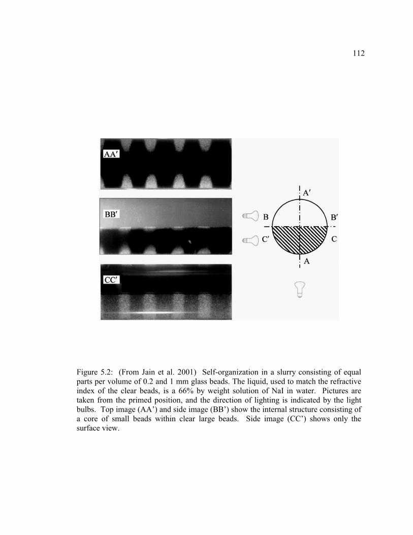
112
Figure 5.2: (From Jain et al. 2001) Self-organization in a slurry consisting of equal
parts per volume of 0.2 and 1 mm glass beads. The liquid, used to match the refractive
index of the clear beads, is a 66% by weight solution of NaI in water. Pictures are
taken from the primed position, and the direction of lighting is indicated by the light
bulbs. Top image (AA’) and side image (BB’) show the internal structure consisting of
a core of small beads within clear large beads. Side image (CC’) shows only the
surface view.

113
refractive index of transparent glass beads, revealing the internal structure of the system
(figure 5.2 – the bi-axial rotation experiment in section 3.4 uses similar particles and
fluid). Top view shows the internal structure consisting of a core of small beads within
large clear beads. Surprisingly, in the systems studied by Jain et al. (2001), axial
segregation occurs faster under slurry conditions than in the corresponding dry systems.
Axial segregation also occurs in cylinders with non-circular cross sections (Hill et
al. 1999b). As seen in chapter 2, flow in a non-circular cross section is chaotic.
Surprisingly, axial bands also form in cylinders with square cross sections, even though
segregation in the cross section is considerably more complex than in the classic cylinder
(figure 5.3). The standard axial segregation pattern is clearly observed in the top of the
flowing layer (figure 5.3a), while two lobes are evident on the bottom view of the mixer
(figure 5.3b), as is seen in the two-dimensional 50% full square (described in chapter 3).
It appears that classical radial segregation is not a necessary condition for axial
segregation. In closer analysis, patterns formed at other fill levels of the square also co-
exist with axial banding (Hill et al. 2001).
The experiments of Zik et al. (1994) are quite relevant to segregation in a sphere.
They examine axial segregation in containers with modifications in geometry along the
axial direction. Two different geometries were considered, one with a periodic variation
in radius alternating thick and thin regions, and the other a helical tube. A difference
should be noted. In both of these contours the rotation is slow, producing discrete
avalanches. In the thick-thin tube, axial segregation is induced in materials that did not
form bands in a straight tube of comparable radius. Smaller beads form bands in the

114
Figure 5.3: Axial segregation observed in a tumbler with square cross section. Views
correspond to orientation shown to the right. (a) - The standard axial segregation pattern
is clearly observed in the top of the flowing layer. (b) - In the bottom view, two lobes are
evident, as is seen in the two-dimensional square mixer.

115
“bellies” and bands of large beads in the “necks”. They report that the location of bands
is reversed at lower fill levels. In the helical tube, material completely segregates to
opposite ends of the container. Another geometry similar to this is a double-cone blender
studied by Alexander et al. (2001), also forming axial bands. Bands of smaller beads
form in the middle of the container at lower rotation rates. This pattern reverses at higher
rotation rates with larger particles forming bands in the middle. These bands coarsen in
time. In both of these studies, the authors suggest that geometry produces a variation in
the angle of repose in the axial direction, aiding in the initiation of axial segregation.
The majority of tumblers used in industry produce some degree of flow in the
axial direction, attempting to destroy segregated structures and enhance mixing. The
geometry and motion of these tumblers is typically complicated (e.g., V-blenders,
double-cones, and cubes – some of these rotated on an oblique axis as shown in figure
5.1). Various mixing studies have been performed in many specific (often patented)
tumblers. Bands formed from axial segregation have not been reported in any tumblers
with periodic axial flow. It is a common assumption that axial mixing inhibits axial
segregation. In attempting to quantify this, Wightman and Muzzio (1998b) perturb flow
in a cylinder with rocking motions, however they only consider a few different
frequencies at low amplitudes. The initial condition is unmixed with each material on
different ends of the container in the axial direction. Their system, without rocking,
produces axial bands. Concentration of material is evaluated after numerous rotations
either by solidifying the granular bed and imaging or by inserting dividers, sieving the
particles, and weighing the amounts as a function of axial distance. With symmetric

116
rocking with amplitude of 5º, the segregation pattern investigated at three different
rocking frequencies is complex. They report segregation in the axial direction, however
there is no evidence of distinct alternating bands. At one frequency, they see progression
towards homogeneous mixing. At another frequency, they see poor axial mixing –
deviating very little from the initial condition. They note that there are higher
concentrations of larger beads near the ends after 1000 rotations. It is unclear whether
these patterns are steady after 1000 rotations or even if distinct bands rise to top of the
flowing layer. In Shinbrot et al. (2001), rocking angles are varied from 0º to 90º.
Concentrations differed along the axis, but once again there is no evidence of axial bands
(except, of course, at 0º).
We investigate 3D mixing and segregation within a sphere. This is a simpler
system than those systems producing 3D flow listed above. The main reason for this is
that in a sphere the free surface remains constant regardless of the orientation. Modeling
of continuous flow within the sphere is also possible. Without rocking, band formation in
a sphere is expected considering the bands that arise in a double-cone blender (Alexander
et al. 2001). In an S-system, smaller beads do form a band in the center of the sphere
(figure 5.4), agreeing with behavior seen by Zik et al. (1994).
5.2 Experimental Details
The experimental apparatus is the same as described in section 3.2. Figure 5.5
shows the experimental setup and rocking protocol. The only modification to this system
from the bi-axial protocol (chapter 3) is to produce simultaneous rotation about two axes.

117
Figure 5.4: Formation of an axial band in a sphere (bottom view). Top – a band
without rocking captured without using a UV filter. Bottom – a coherent band can also
form with rocking. Each band connects through the flowing layer (not shown). From
this perspective, rotation on axis A moves the particles shown from left to right.
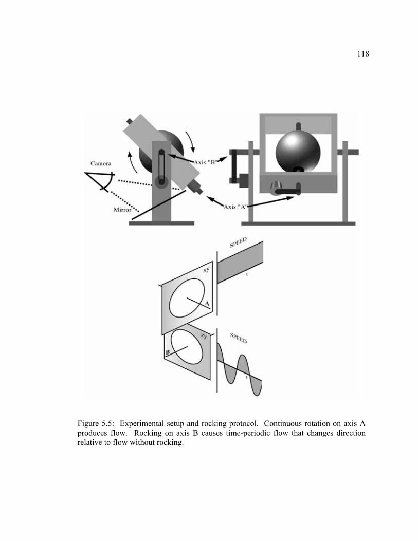
118
Figure 5.5: Experimental setup and rocking protocol. Continuous rotation on axis A
produces flow. Rocking on axis B causes time-periodic flow that changes direction
relative to flow without rocking.

119
The motor control indexer (Compumotor) allows simultaneous control of up to four
motors. It is designed with its own programming language to ensure synchronization of
any combination of these motors. Our system has two motors where a motor produces
motion on each axis. The stepper motors have 25,000 steps per 360º of rotation
providing smooth motion. The first motor rotating axis A has constant angular velocity.
The second produces sinusoidal motion on axis B, where the rocking angle is defined as
( )tA πφγ 2sin= . Rocking is scaled by the constant angular velocity on axis A,
πθω 2// =t and ωφ /=f such that ( )θγ fAsin= . Thus, for 1=f , one rocking cycle
occurs in one full rotation on axis A. The indexer synchronizes all motions with an
internal clock. The coordinates to describe most phenomena in this chapter will be in the
lab frame – the x’, y’, z’ coordinate system described in chapter 4 and shown in figure
4.1; some aspects of the pattern in the flowing layer are described in terms of the frame of
reference relative to the direction of flow (x, y, z).
Patterns arise at the boundary consisting of particles resting against the inside
bottom surface of the tumbler. For clear imaging, most experiments are performed with
larger black beads (2 mm) and smaller fluorescent green beads (0.8 mm) illuminated by
UV lamps. A stationary digital camera captures images of these patterns from below.
Air is the interstitial fluid. The sphere ( mm 140=r ) in most of these experiments is
half-full with granular material and rotated such that the flow is always in the rolling
regime with a flat free surface. The mass ratio between small and large beads is typically
1:2 – there are roughly 500,000 beads in the sphere (estimated from the volume of the

120
sphere, packing fraction and size of individual beads). Most of the results described
below use these materials unless otherwise specified.
A potential difficulty in using S-systems should be noted. It was mentioned in
chapter 3 that size segregation may be more complicated than density segregation. Under
certain conditions, the velocities in the flowing layer are coupled to local concentration.
The flowing layer may become rich in small particles or consist entirely of large
particles. This produces time dependent speeds in the shear layer making S- systems
more complicated than D-systems. While evidence of this sort of coupling is not seen in
our experiments, it is likely to exist at other fill levels or with other materials.
A few experiments are also conducted under slurry conditions, where the
interstitial fluid is water. The radius of the sphere is 40 mm and the particle sizes are 0.8
mm (zirconium silicate) and 0.2 mm (glass), so both size and density are different
( 2/ 21 ≈ρρ ). These particular beads were chosen for clear imaging, however it should
be noted that they segregate quickly in a cylindrical drum forming many axial bands after
just 5 - 10 rotations (Fiedor and Ottino 2003). Size segregation dominates, causing
smaller beads to form a radial core after 1 or 2 rotations before re-emerging at the surface
as bands or other patterns.
Because segregation dominates, initial conditions are never “well-mixed”.
However, the initial distribution of particles in all experiments is set by erratic motions of
the tumbler on its two axes, resulting in each initial condition being unique. Transients
from the initial condition are first destroyed by radial segregation in one or two cycles.

121
In the dry case, it is clear from many repeated experiments that the final segregation
pattern is independent of the initial condition. However, it appears that certain patterns
are transient and dependent on the initial condition in slurry conditions.
5.3 Formation of a Band and Spots
Consider the dry system described above. Rotation on a single axis produces a
stable single band after ~5 minutes of rotation at 5 rpm. In fact, this combination of
materials in this container never produces more than one band. When rocking, the three
most commonly observed patterns are shown in figure 5.6: bands, spots, and no visible
segregation pattern (where all smaller beads segregate away from the walls of the
granular bed). An axial band wraps around the bottom of the granular bed and connects
through the flowing layer. For different frequencies, the band may be very wavy or
relatively straight, however within the flowing layer, it always aligns roughly in the
direction of flow. Also, this band is often observed close to center of the flowing layer at
all times (in the frame of the flowing layer where flow is in the x-direction, it is located at
or near 0=z ). The final pattern begins to emerge after ~20 cycles – roughly the same
amount of time as without rocking. Surprisingly, at certain frequencies, bands are stable
even when rocking angles are greater than 60º. The band either only consists of smaller
beads or consists of both small and large beads (denoted as “diffuse”).
When spots form, the regions may also be well segregated with relatively sharp
boundaries or diffuse. The spots are typically round, but in some cases, they are V-
shaped or four-pointed stars. Typically, they are only seen from the bottom (i.e., only

122
Figure 5.6: Segregation patterns in a rotating-rocking sphere – typical patterns as seen
from the bottom. The bands are either relatively straight or wavy. Spots are located at
various regions at the end of a rocking cycle and sometimes all of the small beads are
segregated to the interior of the granular bed (no pattern).

123
pass through the flowing layer) twice in each rocking cycle at every π /f. It is difficult to
capture images of these spots when they are located at either end of the tumbler and not
at the bottom of the container. All of the patterns produced from sinusoidal rocking are
symmetric; each half cycle has the same pattern as the previous half cycle rotated 180º in
the xz plane. At some frequencies, there is no observable segregation pattern at the
boundaries of the container; all small beads segregate to the center of the granular bed.
5.4 Space-time Plots
Spatio-temporal (space-time) plots are used to display the shape of the pattern at
the boundary throughout an entire rocking cycle. A somewhat similar technique has been
used previously in describing the time evolution of multiple bands in a cylinder. In
cylinders, a digital picture of the bottom of the container is taken after Δt – typically the
time for a single rotation. Each image consists of a thin horizontal part of the picture
(typically 1 line of pixels) simply to capture the number of bands and the width of each
band. These pictures are then stacked as shown in figure 5.7 to represent the evolution of
the pattern in the axial direction in time (time is shown vertically).
The rocking sphere is time-periodic. Therefore, rather than looking at the
temporal evolution of the patterns over multiple cycles, a variation of this technique is
used to capture the shape of the final pattern over an entire rocking cycle. Pictures of the
bottom of the sphere are taken using digital video at 30 frames per second ( s 30/1=Δt ).
At a rotation rate of 5 rpm, 360 pictures are captured – one picture per degree of rotation.
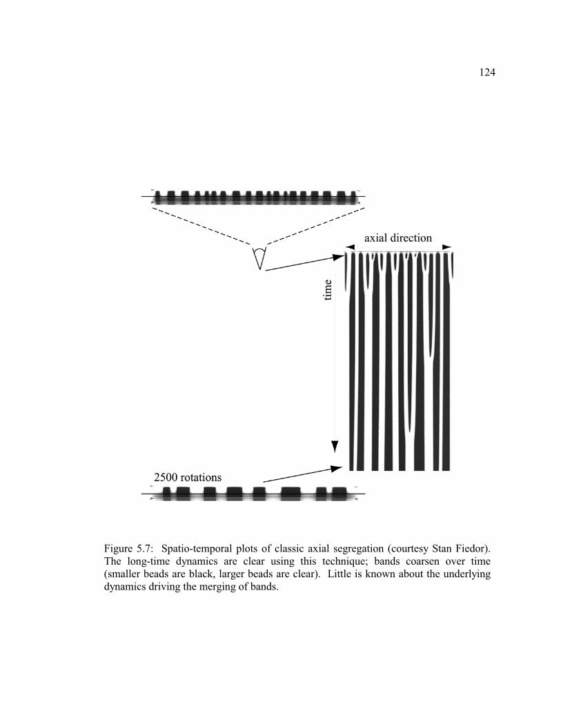
124
Figure 5.7: Spatio-temporal plots of classic axial segregation (courtesy Stan Fiedor).
The long-time dynamics are clear using this technique; bands coarsen over time
(smaller beads are black, larger beads are clear). Little is known about the underlying
dynamics driving the merging of bands.

125
One degree of rotation translates into a distance along the equator of the sphere of
approximately ( ) mm 9.0360/mm 1402360/2 == �� ππr . In each individual digital
picture, this corresponds, roughly, to two pixels. By extracting the two center columns of
pixels from each picture and aligning them sequentially (as shown in figure 5.8), the
segregation pattern is shown in one picture for an entire cycle. An axial band appears as
a straight line (it is almost always located at the bottom of the container) and spots are
periodic regions of smaller beads (bottom). The thin wavy line in this picture is the seam
between two hemispheres of the acrylic container. The smoothness of this line
demonstrates both the continuity of the picture as well as the smoothness of the rocking
motion.
A spatio-temporal image of the container without rocking is analogous to a
cylindrical projection in cartography, mapping the spherical surface of Earth onto a flat
surface (Bugayevskiy and Snyder 1995). The data at the top and bottom of the picture is
skewed such that beads near the ends of the sphere are represented wider and thinner than
reality and are out of focus relative to the center of the picture. With rocking, for
instance, the line representing the seam undergoes almost perfect sinusoidal motion,
however in the image, it is represented by a curve that is roughly sinusoidal, but flattened
at the maxima and minima. Another issue is that parts of the frame of the apparatus
obscure parts of the picture at high values of the amplitude, A. First axis A is in view,
concealing beads behind it. At the highest amplitudes, the platform holding the motor for
axis A significantly blocks the view of the container. Since the larger beads are black

126
Fig
ure
5.8
: C
onst
ruct
ion o
f sp
atio
-tem
pora
l co
mposi
te i
mag
es.
The
cente
r pix
els
of
each
fra
me
from
dig
ital
vid
eo o
f th
e bott
om
vie
w o
f th
e tu
mble
r ar
e cr
opped
. T
hes
e sl
ices
of
the
pic
ture
s ar
e hori
zonta
lly a
ligned
in
tim
e.
Th
e to
p a
nd
bo
tto
m o
f th
e pic
ture
are
z’
= ±
1.
The
dif
fere
nce
bet
wee
n b
ands
and s
pots
is
clea
rly s
een
at t
he
bo
tto
m.

127
and typically are found in these obscured regions, this effect is minimal. Later in this
chapter, in pictures depicting experiments under slurry conditions, the region of the
picture where the apparatus is in view is masked in black (see figures 5.16 and 5.18).
These issues should be taken into account when comparing the experimental results to the
model.
5.5 Phase Diagram
When changing A and f, it is essential to maintain operation within the rolling
regime. However, as the system starts to rock, the Froude number changes in a time-
periodic manner. The Froude number at any instant is defined as
( )( )
gdtdR
Fr
2
22 cos ���
���+
=
γγω. (5.1)
Fr is a function of both rotation rate, ω , rocking angle, γ , and the rate of rocking on axis
B, dtd /γ . Figure 5.9 shows the evolution of Fr during one typical rocking cycle. At
high rocking frequencies and moderate amplitudes, the flow enters the cataracting regime
when axis A is nearly horizontal ( 0=γ at f/,0 πθ = , 221~ fAFr + ) due to the high
accelerations produced by rocking. At the highest amplitudes considered, the flow enters
the discrete avalanching regime at f/90=θ and f/270=θ in the cycle, and when A is
greater than 75º (roughly 90º minus the dynamic angle of repose) the flow temporarily
comes to a stop. At this angle, not enough material advects solid body into the flowing
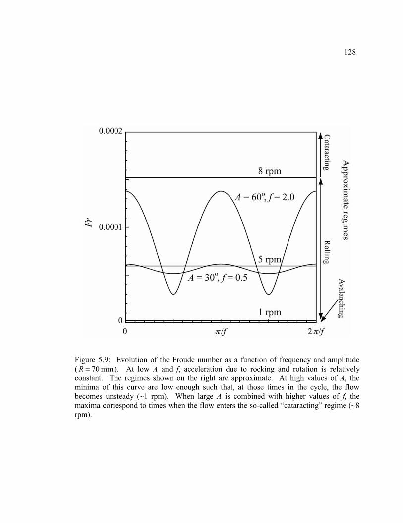
128
Figure 5.9: Evolution of the Froude number as a function of frequency and amplitude
( mm 70=R ). At low A and f, acceleration due to rocking and rotation is relatively
constant. The regimes shown on the right are approximate. At high values of A, the
minima of this curve are low enough such that, at those times in the cycle, the flow
becomes unsteady (~1 rpm). When large A is combined with higher values of f, the
maxima correspond to times when the flow enters the so-called “cataracting” regime (~8
rpm).

129
Fig
ure
5.1
0:
Ser
ies
of
pic
ture
s at
A =
45º.
P
atte
rns
chan
ge
from
no a
ppar
ent
pat
tern
to a
ban
d t
o s
pots
to a
ban
d a
gai
n a
nd o
ther
pat
tern
s at
hig
her
fre
quen
cies
. C
lose
inves
tigat
ion s
how
s th
at t
he
tran
siti
on f
rom
a b
and
to s
pots
is
extr
emel
y s
ensi
tive
to f
requen
cy.

130
layer to sustain continuous flow. Experiments at low frequencies take much longer;
therefore experiments are arbitrarily cut off at 2.0=f .
We wish to explore how amplitude and frequency affect axial banding. Consider
a set of experiments at �45=A (figure 5.10). At 45.0<f , there is no observable
pattern. However, with increasing f, the system displays different patterns (band, no
band, or no pattern). Besides this, as 0→A , banding must be stable for all frequencies
(the no rocking case). These results are reproducible – each experiment is conducted as
few as twice and as many as 20 times. At this point, it is unclear how amplitude and
frequency affects axial banding.
To fully display the effect of rocking amplitude and frequency, a phase diagram is
constructed to map the different patterns (figure 5.11). These results are quite surprising.
Axial banding, the “phase” denoted in gray, is remarkably stable across the region
investigated. The right and top boundaries of this diagram roughly outline where the
flowing layer remains in the rolling regime. Approximately 227 different sets of
parameters (roughly 1000 individual experiments including repetition) were sampled to
construct this diagram. Rocking is relatively insignificant up to �5~A for all
frequencies. This is unlike the rocking cylinder considered by Wightman and Muzzio
1998b) where the highest amplitude considered is �5=A . For increasing amplitude,
there is still a large range of frequencies where an axial band is stable. This region
steadily shrinks with increasing amplitude. At �30≈A , spots are stable for a narrow
range of frequencies near 85.0=f and 2.1=f . The region of stable bands is split at

131
Figure 5.11: Experimental phase diagram with “Arnold tongues”. The pictures in figure
5.10 are performed along the dashed line at �45=A (the bottom line of pictures
corresponds to the focus region in the top right). Stability of a band is surprisingly
sensitive to the frequency and amplitude. Each of 227 data points represents 2-20
experiments and the resolution is smaller than the size of each point.

132
higher amplitudes. An alternate way to characterize the landscape of this map is to
describe the regions where axial banding is not stable. Regions of axial banding
instability grow from ),85.,30( =°= fA ),2.1,30( =°= fA and ).7.1,30( =°= fA
Now reconsider the set of experiments at �45=A described in figure 5.10. This
phase diagram now explains and clarifies what appeared as inconsistent behavior seen in
figure 5.10. If experiments were performed at amplitudes �30<A , the region of spots
would not have been seen. The lack of a band at higher frequencies could have been
construed as simply high enough Froude number such that the flow is unstable.
However, this bifurcation occurs at even higher frequencies at low amplitudes, and
therefore low Froude numbers. From an engineering viewpoint, the above-described
sensitivity to operating parameters is undesirable. It suggests that current geometries
may mix or unmix depending on the precise value of operating conditions. It also
suggests that tumbler designs that cannot be adapted or discarded when tested at only a
few sets of parameters. These transitions may continue at even higher frequencies. As
shown in the phase diagram, spots form at �5=A , 6.1=f , but bands are once again
stable at �5=A , 2=f . It is unclear if more experiments are performed whether these
separate but similar transitions would reveal information about this process.
Consider the overall shape of the phase regions. The shape of this A-f phase
diagram shows structures reminiscent of “Arnold tongues” (figure 5.12 from Hilborn
1994). Arnold (1983) introduced a simple model – the “sine circle map” – to study the
phenomenon of frequency-locking between coupled oscillators. Frequency-locking

133
occurs when two oscillators with nearly commensurate frequencies “lock” when coupled
by weak nonlinear interaction. Two frequencies are considered commensurate when their
ratio, Ω, is rational. Real world examples of this exist in planetary motion (e.g., the same
side of the moon always faces earth) and in the synchronization of mechanical clocks
residing on the same table, first noted by Huygens in 1665 (vibrations in the table provide
the weak nonlinear interaction). In the simple case of two oscillators studied by Arnold,
these nonlinear interactions cause frequency-locking near all rational frequency ratios,
but are strongest near low-order frequency ratios – such as 0:1, 1:1, and 1:2. Denote the
magnitude of the nonlinear interaction as K. When the frequencies are nearly in phase,
the nonlinear interactions are large even for low values of K compared to the difference
in frequencies. This acts to form a “sink” or attractor. The regions in a K- Ω phase map
where oscillators do not frequency-lock are called denoted as “tongues”.
In the experimental phase diagram, f is scaled by full rotations of the tumbler.
Consider a rescaling of our variables in order to draw similarities between the
experimental phase diagram and classic frequency-locking phase diagram (both shown in
figure 5.12). The rocking frequency is scaled by the average circulation time
2//* fT ==Ω ωφ . ½* =T is the dimensionless average circulation time for any half-
full tumbler (defined in section 2.2). A value of 1=Ω corresponds to one rocking cycle
per one circulation of a particle (on average). The rocking is the source of the nonlinear
behavior – a perturbation to simple flow on one axis. Therefore, A is the magnitude of
the nonlinearity – analogous to K in the sine circle map. In the rocking sphere, note the

134
Figure 5.12: Qualitative comparison of experimental phase diagram and frequency-
locking (bottom diagram from Hilborn 1994). Rescaling to compare cycles to material
circulations, 2/f=Ω . There are many similarities between the stability of bands and
the regions that do not frequency-lock. In the rocking sphere, note the regions of spots
growing upward from (f, A) of (0.85, 30�), (1.2, 30�), and (1.7, 5�) corresponding
roughly to ratios of 2:1, 3:1, and 4:1.

135
regions of spots growing upward from (f, A) of (0.85, 30�), (1.2, 30�), and (1.7, 5�).
These correspond roughly to ratios of 2:1, 3:1, and 4:1. It should be noted that further
investigation is likely to reveal another region of frequency-locking in the neighborhood
of (0.43, 30�) corresponding to a 1:1 relationship. While there are many similarities, this
analogy to the sine-circle map is only qualitative.
5.6 Comparison to Computations
Consider now the relationship of the experimental results to the computer
simulations of chapter 4 and appendix A. The model considers flow in a rocking-rotating
sphere. It is important to note that this model only describes advection without
segregation. This is a simplification of the experimental system with a binary material
represented as a single component.
In spite of these caveats, by constructing spatio-temporal pictures from the
computations, direct comparisons are made between model and the experiments. Points
in surface Poincaré maps in chapter 3 are convected and their locations are recorded 180
times throughout one rocking cycle. At each time t during the cycle, the centermost
points ( )180/180/ ππ <<− x are re-plotted z vs. t ( 11 ≤≤− z and φπ /20 ≤≤ t ). As in
the experimental spatio-temporal composites, when the hemispherical surface is projected
onto a flat surface, the chaotic regions near the top and bottom are distorted, typically
making them seem larger in relation to the dynamics in the center.

136
There is qualitative agreement between the shapes of bands seen in experiment
and corresponding Poincaré maps (figure 5.13). This set of spatio-temporal composites
of the experiment (top) and computation (below) at �45=A and 0.1=f show how a
wavy axial band is mimicked by the corresponding quasi-periodic trajectories. The
centermost quasi-periodic trajectories in the Poincaré map are highlighted in green to
assist visualization. For aesthetic reasons and ease of comparison, all of the spatio-
temporal pictures are formatted to the same dimensions. Otherwise, the length of each
picture would be proportional to φπ /2 . The qualitative similarity is striking (see figure
5.13 and 5.14)
There are many frequencies where the model shows periodic points with
surrounding regular regions (figure 5.14), possibly corresponding to spots formed in the
experiment. However, the periodicity of these regular regions does not match the
periodicity of the spots that remain when the band becomes unstable. On the other hand,
at roughly the same frequencies as the experiment, the model does predict a dilation of
the quasi-periodic trajectories where flow stagnates. The periodicity, relative size, and
orientation of these stagnation regions are roughly the same as spots. Experiments in the
dry system at conditions exhibiting the same periodicity as the other Poincaré maps
shown here were not found. It is possible that they exist in a very narrow range of
frequencies or they do not exist at all – the magnitude of the rocking may not produce
large enough perturbations to the flow.

137
Fig
ure
5.1
3:
Qual
itat
ive
com
par
ison b
etw
een a
ban
d i
n t
he
exper
imen
t an
d t
he
shap
e of
the
quas
i-
per
iodic
tra
ject
ori
es i
n t
he
mo
del
A =
45�
and f
= 1
.0.
On t
he
left
, th
e re
d l
ine
dep
icts
the
cente
r
pix
els
sam
ple
d t
hro
ughout
the
cycl
e to
com
pose
the
spat
io-t
empora
l co
mposi
te o
n t
he
right.
T
he
cente
rmost
quas
i-per
iodic
tra
ject
ori
es i
n t
he
model
are
shad
ed i
n g
reen
.

138
Figure 5.14: Comparison between regular regions in model and spots in experiments.
From top to bottom: (A = 40�, f = 1.5), (A = 45�, f = 0.6), (A = 45�, f = 0.957), and the
experiment is at (A = 45�, f = 0.842). In the model, regular regions of various
periodicity exist, however in this experimental system only spots with the bottom
periodicity are seen.

139
Consider now the narrow range of frequencies where the band bifurcates into
spots and back into bands (shown in figure 5.10). Closer investigation of this bifurcation
is possible by creating successive spatio-temporal plots of the patterns at frequencies
between 824.0=f and 856.0=f (figure 5.15). The band appears to “pinch-off” at
distinct times in the rocking cycle. After pinch-off, these spots contract. At slightly
higher frequencies, these spots stretch out back into bands. Interestingly, these spots are
at the same location within the cycle where the bands originally pinched-off at lower
frequencies. The bands initially break in the cycle when 0=γ . The spots, originally
located at 0/ =θγ dd , migrate to this part of the cycle when 0=γ . It should be noted
that this pinch-off is not a dynamic process, as each of these pictures is the final
segregation pattern after many rocking cycles in separate experiments.
Alongside the experimental pictures in figure 5.15, the computations from figure
4.12 are shown as spatio-temporal plots. The transition over this narrow range of
frequencies is similar. The phase-shift seen in the experiments is mimicked in these
consecutive plots. The quasi-periodic trajectories become wavy, dilating at one point in
the cycle and necking at another. At a specific frequency, two hyperbolic points exist in
the region where trajectories are dilating. These points drift apart as the frequency
increases. Because of the periodicity of the flow, as a pair of hyperbolic points drifts
apart, one approaches the hyperbolic point associated with the previous cycle and the
other approaches a hyperbolic point associated with the next cycle. The hyperbolic
points in each new pairing converge. They eventually annihilate each other, creating a
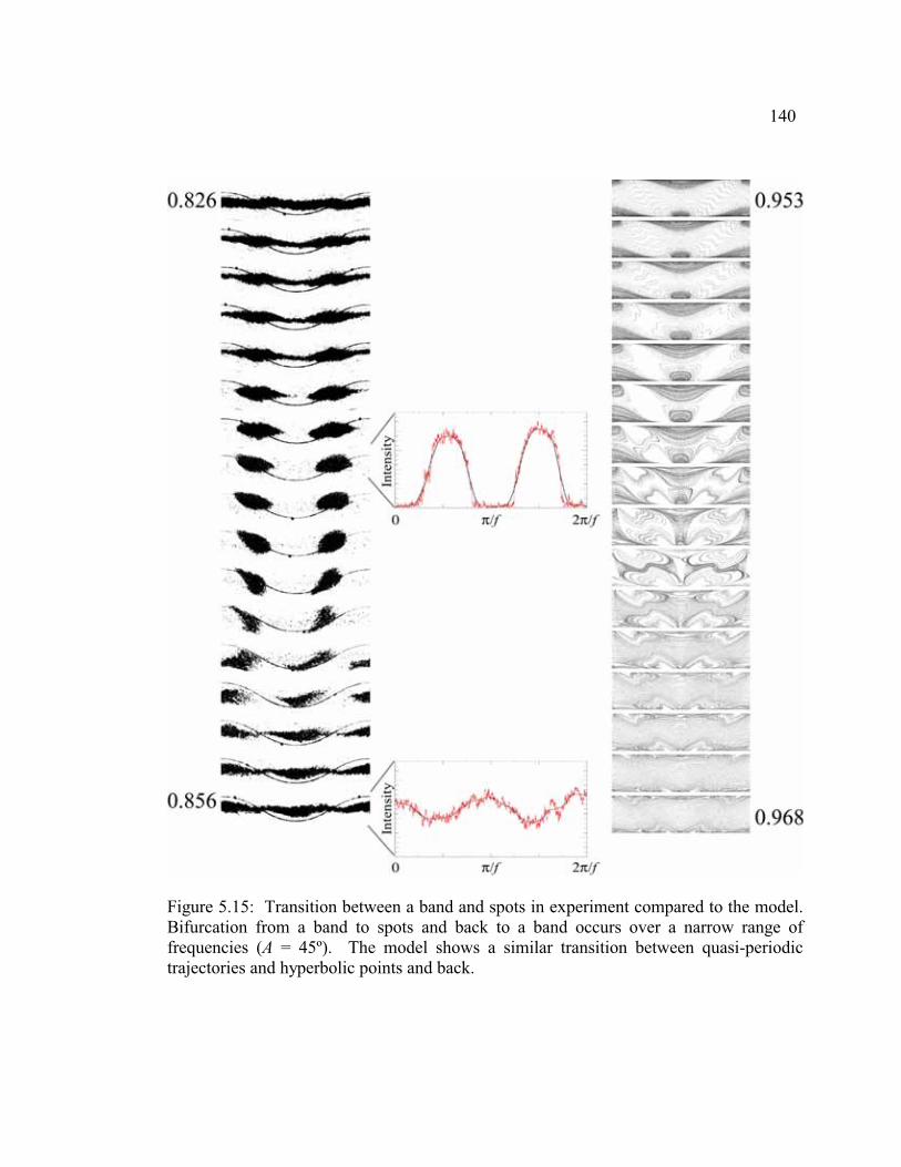
140
Figure 5.15: Transition between a band and spots in experiment compared to the model.
Bifurcation from a band to spots and back to a band occurs over a narrow range of
frequencies (A = 45º). The model shows a similar transition between quasi-periodic
trajectories and hyperbolic points and back.

141
part of the flow where quasi-periodic trajectories once again exist in the center of the
map. These quasi-periodic trajectories once again have regions where they diverge and
contract as seen at frequencies lower than the bifurcation, however the regions have an
apparent phase-shift of 90º compared to pictures at lower frequencies.
This bifurcation is remarkably similar to the transition from a band to spots and
back to a band. The model, without modeling segregation, may be used to investigate the
range over which the band is unstable and the phase-shift of spots throughout the
transition. The most remarkable aspect of this correspondence is that this happens even
though the dry S-systems considered in this particular example are, in general,
significantly more taxing from a modeling standpoint than the corresponding D-systems
(as mentioned in section 3.3.2). However, if no significant time effects arise from the
flow composition in the layer, as is the case in the experiments reported here, the system,
once in steady state, behaves essentially as a single fluid and can be modeled as such.
This model does not directly predict frequency-locking, as suggested by the
experimental phase diagram. The hyperbolic points in the surface Poincaré maps in
figure 5.15 are created via period-doubling. Like frequency-locking, periodic points exist
in the map when the frequencies associated with rocking and circulation are
commensurate. A represents the magnitude of the nonlinear terms, and increasing A
increases the range where periodic points exist. Although this mechanism is very similar,
there are distinct differences between period-doubling and frequency-locking. For
instance, sources and sinks required to produce frequency-locking cannot exist in a
volume-preserving model.
142
However, constitutive equations describing axial segregation are not available.
However, consider the relationship between radial segregation and the underlying flow,
described in chapter 3. It is noted that the regular regions behave as “attractors” for one
type of material when the system is still well mixed – materials preferentially segregate to
opposite regions of the flow. The system could be viewed as two co-existing maps, each
associated with one material. These two maps would have matching sets of sinks and
sources driving the two materials into different regions of the flow. The strength of these
sinks and sources would be relative to local concentration and proportional to differences
in material properties driving segregation. When materials reach a final segregated state,
segregation only exists at the phase boundaries. Inside each phase, the materials are
mono-disperse and flow as described by the model. The phase boundaries have no force
analogous to surface tension in liquids, therefore they must follow along the underlying
invariant structures produced by flow of each mono-disperse material – as suggested in
chapter 3 in two-dimensional systems. If sources and sinks do exist, this allows the
possibility of frequency-locking suggested in the experimental phase diagram. Once
again, this suggests that final segregation patterns are independent of material properties
causing segregation. If this is true, then the same phenomena should also exist under
slurry conditions (analogous to the dry and slurry conditions tested in bi-axially rotated
cubes shown in figure 3.17).
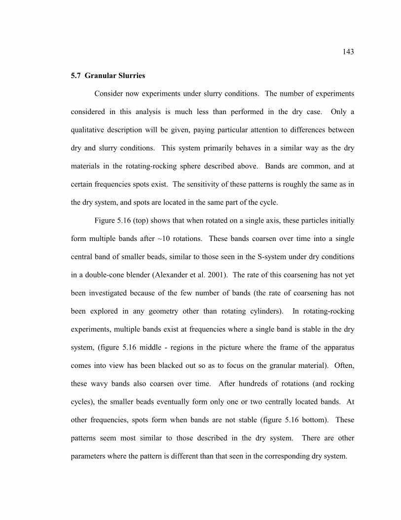
143
5.7 Granular Slurries
Consider now experiments under slurry conditions. The number of experiments
considered in this analysis is much less than performed in the dry case. Only a
qualitative description will be given, paying particular attention to differences between
dry and slurry conditions. This system primarily behaves in a similar way as the dry
materials in the rotating-rocking sphere described above. Bands are common, and at
certain frequencies spots exist. The sensitivity of these patterns is roughly the same as in
the dry system, and spots are located in the same part of the cycle.
Figure 5.16 (top) shows that when rotated on a single axis, these particles initially
form multiple bands after ~10 rotations. These bands coarsen over time into a single
central band of smaller beads, similar to those seen in the S-system under dry conditions
in a double-cone blender (Alexander et al. 2001). The rate of this coarsening has not yet
been investigated because of the few number of bands (the rate of coarsening has not
been explored in any geometry other than rotating cylinders). In rotating-rocking
experiments, multiple bands exist at frequencies where a single band is stable in the dry
system, (figure 5.16 middle - regions in the picture where the frame of the apparatus
comes into view has been blacked out so as to focus on the granular material). Often,
these wavy bands also coarsen over time. After hundreds of rotations (and rocking
cycles), the smaller beads eventually form only one or two centrally located bands. At
other frequencies, spots form when bands are not stable (figure 5.16 bottom). These
patterns seem most similar to those described in the dry system. There are other
parameters where the pattern is different than that seen in the corresponding dry system.

144
Fig
ure
5.1
6:
Exper
imen
ts u
nder
slu
rry c
ondit
ions.
T
op i
s an
exper
imen
t w
ithout
rock
ing w
her
e
mult
iple
ban
ds
are
form
ed.
Mid
dle
show
s m
ult
iple
ban
ds
wit
h r
ota
ting a
nd r
ock
ing (
A =
45º,
f =
0.9
67
).
Bo
tto
m s
ho
ws
spo
ts (
A =
10º,
f =
1.6
7).
In
the
mid
dle
pic
ture
, a
bla
ck m
ask i
s use
d t
o
cover
the
area
wher
e th
e fr
ame
of
the
appar
atus
com
es i
nto
vie
w.

145
Some of these experiments produce bands that apparently fork into multiple bands
(figure 5.17 top). The stability of these bands is unclear. While a central band always
exists, after splitting, one of the branches ends abruptly. Band formation and
disappearance on the order of a single rotation has not been previously reported. It is
unclear if this is the final pattern.
At the same amplitude but higher frequency, wavy bands are stable, but the
smaller beads now migrate to the ends of the sphere and larger beads form the bands in
the middle (figure 5.17b). This phenomenon (referred to as “big-out”) is observed in a
double-cone blender (Alexander et al. 2001) by changing the rotation rate of the tumbler.
Preliminary experiments suggest that this “big-out” pattern may depend on the initial
condition. The pattern is reproducible when starting with a mixed initial condition (in
which the tumbler is rotated quickly and a mixture of small and large particles exist at the
bottom of the container) and is stable for many hundreds of cycles. However, when the
initial condition is a leftover pattern from another experiment, bands form, but smaller
beads may once again form the bands in the center of the tumbler (also stable for
hundreds of cycles). The pattern itself does not seem to be a transient effect – bands are
consistently formed in both cases.
Another qualitative difference between the dry and slurry conditions is the
number of spots. In the dry case, no more than two spots per rocking cycle have been
observed. However, six spots can form under the slurry condition at �40=A and
33.1=f (figure 5.18). The model captures this pattern at �40=A and 5.1=f . The

146
Fig
ure
5.1
7:
Odd p
atte
rns
under
slu
rry c
ondit
ions.
T
he
top (
A =
10º,
f =
1.1
7)
corr
esponds
to a
pat
tern
that
, in
spit
e of
appea
ring p
erio
dic
, m
ay n
ot
hav
e re
ached
a f
inal
sta
te y
et.
The
bott
om
pic
ture
(A
= 1
0º,
f =
1.3
33)
dep
icts
rev
erse
axia
l se
gre
gat
ion,
wher
e th
e la
rger
bea
ds
form
ban
ds
in
the
cente
r of
the
spher
e.

147
Fig
ure
5.1
8:
Model
and s
lurr
y e
xper
imen
t (t
he
par
amet
ers
are
A =
40�,
f =
1.5
and A
= 4
0�,
f_=
_1.3
33 r
espec
tivel
y),
both
dis
pla
yin
g p
erio
d-6
per
iodic
poin
ts.
This
is
not
seen
in t
he
dry
syst
em.
This
sugges
ts t
hat
the
slurr
y m
ay b
e m
ore
sen
siti
ve
to t
he
forc
ing.
In t
he
exper
imen
t, a
bla
ck m
ask c
over
s th
e ar
ea w
her
e th
e fr
ame
of
the
appar
atus
cover
s par
t of
the
spher
e.

148
spots in the slurry are very small and diffuse, but clearly segregate to the same region as
the regular regions in the model. This suggests that using beads with different material
properties possibly could reflect more details of the computed invariant structures. The
spatio-temporal picture of this is less clear than the still images because these spots are
small. At this rocking amplitude, axis A is visible, and covers part of the bottom view of
the granular bed. Again, the area where the frame of the apparatus comes into view has
been blacked out so as to focus on the granular material.
5.8 Rocking Cubes
Replacing the sphere with a cube makes the flow significantly more complicated.
Only the basic elements of this system are described here. In all protocols investigated
thus far, the forcing of the system is either periodic with rotation or periodic with rocking
frequency. This system is a combination of both. Consider holding the cube face-
centered by an axis of rotation. A cube is invariant to 90� rotations and multiples thereof.
In a rocking cube, this means the flow can only be periodic at rocking frequencies of
4/* nf = where n is a positive integer.
At all other frequencies, the forcing is quasi-periodic. This is analogous to
rocking the sphere according to a quasi-periodic function, however the shape of the free
surface in a cube is also quasi-periodic (the free surface is an ever-changing polygon). A
rocking cylinder (considered in experiments by Wightman et al. 1998a,b) also has a
periodic free surface shape (the shape free surface in a half-full cylinder ranges from a

149
rectangle when 0=γ to an ellipse roughly when ( )WR /tan 1−>γ where W is the half
width of the main axis of rotation), but it is always periodic with the rocking frequency.
One other consideration: the flow in a cube depends on the initial orientation of the cube
at the beginning of the experiment. A cycle that starts with the free surface parallel to a
side of the cube should give different results than one that starts with the free surface
crossing a diagonal of the cube and so on.
Consecutive pictures of a rotating-rocking cube show segregation patterns (figure
5.19). Because of the geometry, spatio-temporal pictures are impractical. In a cube
rocking with f = 1, a steady pattern forms, and this pattern has similar qualities as both
axial banding and spots. The smaller fluorescent beads do not reach the boundaries.
Some analogies may be made between what is seen in the bi-axial experiments, where
smaller and denser material is located away from the chaotic region in center of the cube.
When the ratio of rocking frequency to circulation rate is quasi-periodic, no
“final” segregation pattern can form. Pictures show that the smaller beads can even
migrate towards the edges of the container, producing reverse axial segregation (figure
5.20). However, this is temporary. Later, the smaller material congregates in the center
of the tumbler. Because of this, each type of material is able to explore most of the
granular bed. This may enhance practical processes such as spray coating, where it
would be beneficial for all material to eventually reside on the free surface. Also,
because the pattern is dynamic, the material properties may also interplay with the
segregation pattern. Altering the magnitude of radial or axial segregation, for instance by
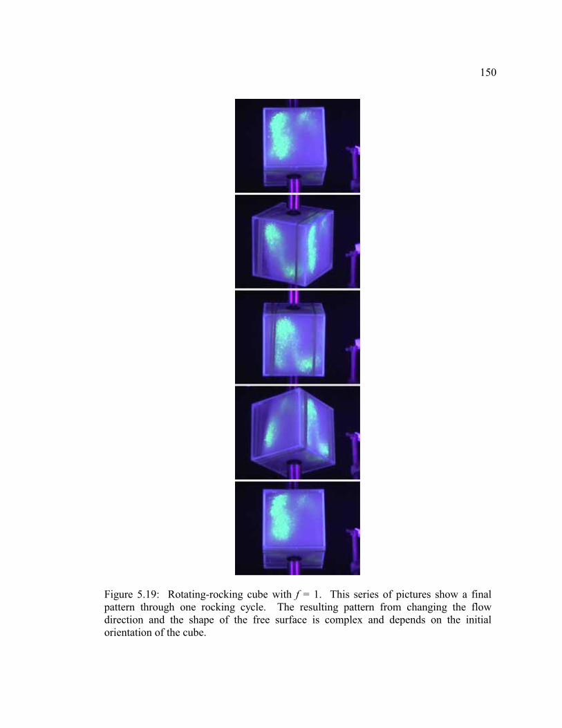
150
Figure 5.19: Rotating-rocking cube with f = 1. This series of pictures show a final
pattern through one rocking cycle. The resulting pattern from changing the flow
direction and the shape of the free surface is complex and depends on the initial
orientation of the cube.

151
Figure 5.20: Rotating-rocking cube with 8.0≈f . This series of pictures shows the
segregation pattern over one rocking cycle. Momentarily, the smaller beads are segregating to the edges of the cube. After a few cycles, the pattern will look different
– the free surface shape is quasi-periodic.

152
performing the same experiments under slurry conditions, may alter a delay in the system
to evolve from one pattern to another.
As container shapes, materials, and flow become more complicated, it is unclear
how well models of the underlying flow will predict segregation structures. As in all
continuum models, the assumptions break down at extreme limits. For example, a
breakdown occurs when the flow velocities become coupled with concentration, as seen
with the streaks formed in the 55% full S- system square in figure 3.10. When this is not
the case, the continuum models of flow of mono-disperse beads used throughout this
dissertation are remarkably accurate in predicting the qualitative segregation patterns.

153
CHAPTER 6
SUMMARY AND OUTLOOK
This dissertation explores granular mixing and segregation in various geometries.
Segregation in a circle is simple. Changing the geometry from simple flow in a circle to
chaotic flow in other shapes has a large effect on the resulting segregation. Invariant
regions in the underlying flow dictate the shape of the phase boundary between materials
differing by physical properties. Both the flow and resulting pattern formation are found
to be sensitive to fill level. In a bi-axially rotated sphere and cube, chaos is generated,
but it is unclear how the resulting segregation patterns relate to the underlying flow.
However, incorporating collisional diffusion and segregation into the model correctly
predicts both simple radial segregation in a sphere and a three-lobe pattern that forms in a
cube.
A simple model of underlying flow in a rotating-rocking sphere demonstrates how
regular regions and chaos are sensitive to the rocking frequency and amplitude.
Experiments within a spherical tumbler produce an axial segregated band when rotated
on a single axis and this band is surprisingly stable when the flow is perturbed with the
addition of rocking. The underlying principles of axial segregation are poorly
understood, but by predicting the sensitivity of the underlying flow to the amplitude and
frequency of rocking, the shape and stability of this band are predicted qualitatively. In
both the bi-axial sphere and cube and rotating-rocking sphere, experiments under both
154
dry and slurry conditions mostly exhibit the same patterns, suggesting that the final
segregation patterns are independent of material properties. It is unclear whether this is
true in a rocking cube, where flow can be quasi-periodic and shape of the segregated
region would likely continuously evolve with the underlying flow.
It is evident that throughout this dissertation there is a rough correspondence
between the model and the experimental results. The most remarkable aspect of the
correspondence is the similarity that is seen even in the dry S-systems which are often
significantly more taxing from a modeling standpoint than the corresponding D-systems
(as mentioned in section 3.3.2). However, if no significant time effects arise from the
composition in the flowing layer, as is the case in the experiments reported here, the
system, once in steady state, behaves essentially as a single fluid, and can be modeled as
such.
It is clear that our model works well under these conditions. This is unexpected,
as the model does not contain segregation. How can we then rationalize the agreement
between experiments and computations? The answer becomes apparent once one realizes
that segregated regions are invariant regions – segregated domains are mapped onto
themselves. Segregation, once completed, has to follow the template provided by the
Poincaré map. It is also obvious that the only place where segregation takes place is in
the layer itself, since is it the only place with non-zero shear rates; in fact the layer is the
only point of entry of materials into segregated domains. Testaments to this are seen
throughout this dissertation.

155
Short of developing constitutive equations, there are many routes to further
understanding of granular flow and segregation. Currently, most research focuses on
existing prototypical systems. However, it is likely that many simple experiments,
analogous to those described in this dissertation, have yet to be discovered. Granular
research is still in a “discovery” phase. New phenomena emerge within novel
experiments that stretch the understanding of granular dynamics past its current
boundaries, and these new phenomena will likely give opportunity to observe and
quantify poorly understood fundamental processes such as axial segregation.
Aside from studying systems exhibiting different behavior, in general it is
necessary to further develop tools of investigation. With more sophisticated scanning
and imaging techniques, it may be possible to automate analysis of granular systems.
One can imagine a feedback system where a segregation pattern is interpreted through
image analysis and this information is then used to alter parameters of the system, such as
rotation rate or rocking frequency. Most of the results presented here are largely
independent of material properties, however systems are difficult to explain when local
concentration couples with the flow. If material parameters could be tuned during an
experiment, the flow and the resulting segregation pattern could be controlled. With the
emergence of nanotechnology, it is even possible that intelligent tools of analysis will
eventually be embedded within the material itself – perhaps tumbling spherical
microchips and analyzing the data of the network of interactions when segregation is
present.

156
REFERENCES
Alexander A.W., Shinbrot T., and Muzzio F.J. 2001. Granular segregation in the double-
cone blender: transitions and mechanisms. Physics of Fluids 13: 578-587.
Aranson I.S. and Tsimring L.S. 1999. Dynamics of axial separation in long rotating
drums. Physical Review Letters 82: 4643-4646.
Arnold V.I. 1983. Geometric methods in the theory of ordinary differential equations.
New York: Springer-Verlag.
Bagnold R.A. 1954. Experiments on a gravity-free dispersion of large solid spheres in a
Newtonian fluid under shear. Proceedings of the Royal Society of London Series A 225: 49-63.
Bridgewater J. 1995. Particle technology. Chemical Engineering Science 50:4081-4089
Bugayevskiy L.M. and Snyder J.P. 1995. Map projections: a reference manual. London:
Taylor and Francis.
Choo K., Baker M.W., Molteno T.C.A, and Morris S.W. 1998. Dynamics of granular
segregation patterns in a long drum mixer. Physical Review E 58: 6115-6123.
Choo K., Baker M.W., Molteno T.C.A, and Morris S.W. 2002. in preparation.
Danckwerts P.V. 1952. The definition and measurement of some characteristics of
mixtures. Applied Scientific Research A3: 279-296.
Das Gupta S., Bhatia S.K., and Khakhar D.V. 1991. Axial segregation of particles in a
horizontal rotating cylinder. Chemical Engineering Science 46: 1513-1517.
Duran J. 2000. Sands, powders, and grains: an introduction to the physics of granular materials. New York: Springer-Verlag.
Elperin T. and Vikhansky A. 1998a. Kinematics of the mixing of granular materials in
slowly rotating containers. Europhysics Letters 44: 17-22.
Elperin T. and Vikhansky A. 1998b. Granular flow in a rotating cylindrical drum.
Europhysics Letters 42: 619-623.
Elperin T. and Vikhansky A. 2000. Granular flow in a three-dimensional rotating
container. Physical Review E 62: 4446-4449.

157
Elperin T. and Vikhansky A. 2002. Variational model of granular flow in a three-
dimensional rotating container. Physica A 303: 48-56.
Fiedor S. and Ottino J.M. 2003. in preparation.
Franjione J.G. and Ottino J.M. 1992. Symmetry concepts for the geometric analysis of
mixing flows. Philosophical Transactions of the Royal Society of London Series A 338: 301-323.
Henein H., Brimacombe J.K., and Watkinson A.P. 1983. Experimental study of
transverse bed motion in rotary kilns. Metallurgical Transactions B 14: 191-205.
Hilborn R.C. 1994. Chaos and nonlinear dynamics. New York: Oxford University Press.
Hill K.M. and Kakalios J. 1994. Reversible axial segregation of binary mixtures of
granular materials. Physical Review E 49: R3610-R3613.
Hill K.M., Caprihan A., and Kakalios J. 1997. Bulk segregation in a rotated granular
material measured by magnetic resonance imaging. Physical Review Letters 78:
50-53.
Hill K.M., Gilchrist J.F., Khakhar D.V., McCarthy J.J., and Ottino J.M. 1999a. Mixing of
granular materials: a test-bed dynamical system for patter formation. International Journal of Bifurcation and Chaos 9:1467-1484.
Hill K.M., Khakhar D.V., Gilchrist J.F., McCarthy J.J., and Ottino J.M. 1999b.
Segregation-driven organization in chaotic granular flows. Proceedings of the National Academy of Sciences 96:11701-11706.
Hill K.M., Jain N., and Ottino J.M. 2001. Modes of granular segregation in a noncircular
rotating cylinder. Physical Review E 64: 1-4.
Jaeger H.M. and Nagel S.R. 1992. Physics of the granular state. Science 255: 1523-1531.
Jaeger H.M., Nagel S.R., and Behringer R.P. 1996a. The physics of granular materials.
Physics Today 49: 32-38.
Jaeger H.M., Nagel S.R., and Behringer R.P. 1996b. Granular solids, liquids, and gases.
Reviews of Modern Physics 68:1259-1273.
Jain N., Khakhar D.V., Lueptow R.M., and Ottino J.M. 2001. Self-organization in
granular slurries. Physical Review Letters 86: 3771-3774.

158
Jain N., Ottino J.M., and Lueptow R.M. 2002. An experimental study of the flowing
granular layer in a rotating tumbler. Physics of Fluids 14: 572-582.
Jain N., Ottino J.M., and Lueptow R.M. 2003. in preparation.
Khakhar D.V., McCarthy J.J., and Ottino J.M. 1997a. Radial segregations of materials in
rotating cylinders. Physics of Fluids 9:3600-3614.
Khakhar D.V., McCarthy J.J., Shinbrot T., and Ottino J.M. 1997b. Transverse flow and
mixing of granular materials in a rotating cylinder. Physics of Fluids 9:31-43.
Khakhar D.V., McCarthy J.J., Gilchrist J.F., and Ottino J.M. 1999a. Chaotic mixing of
granular materials in 2D tumbling mixers. Chaos 9: 195-205.
Khakhar D.V., McCarthy J.J., and Ottino J.M. 1999b. Mixing and segregation of granular
materials in chute flows. Chaos 9:594-610.
Khakhar D.V., Orpe A.V., and Ottino J.M. 2001a. Surface granular flows: two related
examples. Advances in Complex Systems 4: 407-417.
Khakhar D.V., Orpe A.V., and Ottino J.M. 2001b. Continuum model of mixing and size
segregation in a rotating cylinder: concentration-flow coupling and streak
formation. Powder Technology 116: 232-245.
Khakhar D.V., Orpe A.V., Andresen P., and Ottino J.M. 2001c. Surface flow of granular
materials: model and experiments in heap formation. Journal of Fluid Mechanics
441: 255-264.
Lacey P.M. 1954. Developments in the theory of particle mixing. Journal of Applied Chemistry 4:257-268.
McCarthy J.J., Shinbrot T., Metcalfe G., Wolf J.E., and Ottino J.M. 1996. Mixing of
granular materials in slowly rotated containers. American Institute of Chemical Engineers Journal 42: 3351-3363.
Makse H.A., Havlin S., King P.R., and Stanley H.E. 1997. Spontaneous stratification in
granular mixtures. Nature 386: 379-382.
Metcalfe G., Shinbrot T., McCarthy J.J., and Ottino J.M. 1995. Avalanche mixing of
granular solids. Nature 374: 39-41.
Metcalfe G. and Shattuck M. 1996. Pattern formation during mixing and segregation of
flowing granular materials. Physica A 233:709-717.

159
Nakagawa M., Altobelli S.A., Caprihan A., Fukushima E., and Jeong E.K. 1993. Non-
invasive measurements of granular flows by magnetic resonance imaging.
Experimental Fluids 16: 54-60.
Nakagawa M. 1994. Axial segregation of granular flows in a horizontal rotating cylinder.
Chemical Engineering Science 49: 2540-2544.
Nakagawa M., Altobelli S.A., Caprihan A., and Fukushima E. 1997. NMRI study: axial
migration of radially segregated core of granular mixtures in a horizontal rotating
cylinder. Chemical Engineering Science 52: 4423-4428.
Orpe A.V. and Khakhar D.V. 2001. Scaling relations for granular flow in quasi-two-
dimensional rotating cylinders. Physical Review E 64:
Ottino J.M. 1989. The kinematics of mixing: stretching, chaos, and transport. Cambridge,
UK: Cambridge University Press.
Ottino J.M. and Khakhar D.V. 2000. Mixing and segregation of granular materials.
Annual Review of Fluid Mechanics 32: 55-91.
Oyama Y. 1939. Bull. Inst. Phys. Chem. Res.5: 600
Rajchenbach J. 1990. Flow in Powders: from discrete avalanches to continuous regime.
Physical Review Letters 65: 2221-2224.
Rajchenbach J., Clément E., and Duran J. 1995. Experiments in model granular medial a
study of gravity flows. In Fractal Aspects of Materials, edited by F. Family, P.
Meakin, B. Sapoval, and R. Wool, 525. Pittsburgh: MRS Symposium.
Savage S.B. 1993. Disorder, diffusion and structure formation in granular flow. In
Disorder and Granular Media, eds. D. Bideau and A. Hansen, 255-285.
Amsterdam: Elsevier Science.
Shinbrot T., Zeggio M., and Muzzio F.J. 2001. Computational approaches to granular
segregation in tumbling blenders. Powder Technology 116: 224-231.
Swanson P.D. and Ottino J.M. 1990. A comparative computational and experimental
study of chaotic mixing of viscous fluids. Journal of Fluid Mechanics 213: 227-
249.
Umbanhowar P.B., Melo F., and Swinney H.L. 1996. Localized excitations in a vertically
granular layer. Nature 382: 793-796.

160
Wightman C., Muzzio F.J., and Wilder J. 1996. A quantitative image analysis method for
characterizing mixtures of granular materials. Powder Technology 89: 165-176.
Wightman C. and Muzzio F.J. 1998a. Mixing of granular material in a drum mixer
undergoing rotational and rocking motions. I. Uniform particles. Powder Technology 98: 113-124.
Wightman C. and Muzzio F.J. 1998b. Mixing of granular material in a drum mixer
undergoing rotational and rocking motions. II. Segregating particles. Powder Technology 98: 125-134.
Zik O., Levine D., Lipson S.G., Shtrikman S., and Stavans J. 1994. Rotationally induced
segregation of granular materials. Physical Review Letters 73: 644-647.

161
APPENDIX A
The following figures are Poincaré maps produced by the model detailed in
chapter 4. Each individual figure consists of 40 maps, each of which represent
computations at the same amplitude, A, with frequency ranging from 475.15.0 ≤≤ f .
Overall, these took roughly 500 hours of computational time (Pentium IV, 2.4GHz) plus
additional time to plot maps. Many more computations not shown investigate specific
regions (as seen in figures 4.10, 4.11, and 4.12). It is useful to find a specific pattern,
note its amplitude and frequency, and then inspect figures of neighboring amplitudes
(figures) to see if that pattern arises again at the same or nearby frequency. Many
features exist that do not have a specific trend because their range of stable frequencies
are narrower than 0.025.

162
A.1: Computations of a rocking sphere for A = 5º and 0.5 � f < 1.5.

163
A.2: Computations of a rocking sphere for A = 10º and 0.5 � f < 1.5.

164
A.3: Computations of a rocking sphere for A = 15º and 0.5 � f < 1.5.

165
A.4: Computations of a rocking sphere for A = 20º and 0.5 � f < 1.5.

166
A.5: Computations of a rocking sphere for A = 25º and 0.5 � f < 1.5.

167
A.6: Computations of a rocking sphere for A = 30º and 0.5 � f < 1.5.

168
A.7: Computations of a rocking sphere for A = 35º and 0.5 � f < 1.5.

169
A.8: Computations of a rocking sphere for A = 40º and 0.5 � f < 1.5.

170
A.9: Computations of a rocking sphere for A = 42.5º and 0.5 � f < 1.5.

171
A.10: Computations of a rocking sphere for A = 45º and 0.5 � f < 1.5.

172
A.11: Computations of a rocking sphere for A = 47.5º and 0.5 � f < 1.5.

173
A.12: Computations of a rocking sphere for A = 50º and 0.5 � f < 1.5.

174
A.13: Computations of a rocking sphere for A = 52.5º and 0.5 � f < 1.5.

175
A.14: Computations of a rocking sphere for A = 55º and 0.5 � f < 1.5.

176
A.15: Computations of a rocking sphere for A = 60º and 0.5 � f < 1.5.

177
A.16: Computations of a rocking sphere for A = 70º and 0.5 � f < 1.5.