Note 14 of 5E

Statistics with Economics and Statistics with Economics and Business ApplicationsBusiness Applications

Chapter 12 Multiple Regression Analysis

A brief exposition

Note 14 of 5E

IntroductionIntroduction• We can use the same basic ideas in simple linear

regression to analyze relationships between a dependent variable and several independent variables

• Multiple regression is an extension of the simple linear regression for investigating how a response y is affected by several independent variables, x1, x2, x3,…,

xk.

• Our objective are – find relationships between y and x1, x2, x3,…, xk

– predict y using x1, x2, x3,…, xk

Note 14 of 5E

ExampleExample• Fatness (y) may depend on

– x1 = age– x2 = sex– x3 = body type

• Monthly sales (y) of the retail store may depend on– x1 = advertising expenditure– x2 = time of year– x3 = state of economy– x4 = size of inventory

Note 14 of 5E

Some QuestionsSome Questions• Which of the independent variables are useful and

which are not?

• How could we create a prediction equation to allow us to predict y using knowledge of x1, x2, x3 etc?

• How strong is the relationship between y and the independent variables?

• How good is this prediction?

Note 14 of 5E

The General Linear ModelThe General Linear Model

y = y = xx11 + + xx22 +…+ +…+ kkxxkk + +

y is the dependent variable. k k are unknown parameters xxxxxxk k are independent predictor variablesThe deterministic part of the model,

E(y) = E(y) = xx11 + + xx22 +…+ +…+ kkxxkk ,, describes average value of y for any fixed values of

xxxxxxk k . The observation y deviates from the deterministic model by an amount

isisrandom error. We assume random errors are random error. We assume random errors are independent normal random variables with mean zero independent normal random variables with mean zero and a constant variance and a constant variance 22

Note 14 of 5E

The Method of Least SquaresThe Method of Least Squares

• Data: n observations on the response y and the independent variables, x1, x2, x3, …xk.

• The best-fitting prediction equation is

• We choose our estimates to minimize

• The computation is usually done by a computer

2110

2 )ˆ...ˆˆ()ˆ(SSE kk xxyyy 2

1102 )ˆ...ˆˆ()ˆ(SSE kk xxyyy

kk xxy ˆ...ˆˆˆ 110 kk xxy ˆ...ˆˆˆ 110

k ˆ,,ˆ0

Note 14 of 5E

Steps in Regression AnalysisSteps in Regression AnalysisWhen you perform multiple regression analysis, use a step-by step approach:

1. Fit the model to data – estimate parameters.

2. Use the analysis of variance F test and R2 to determine how well the model fits the data.

3. Check the t tests for the partial regression coefficients to see which ones are contributing significant information in the presence of the others.

4. Use diagnostic plots to check for violation of the regression assumptions.

5. Proceed to estimate or predict the quantity of interest

Note 14 of 5E

ExampleExampleA data contains the selling price y (in thousands of dollars), the amount of living area x1 (in hundreds of square feet), and the number of floors x2, bedrooms x3, and bathrooms x4, for n = 15 randomly selected residences currently on the market.

Property y x1 x2 x3 x4

1 69.0 6 1 2 1

2 118.5 10 1 2 2

3 116.5 10 1 3 2

… … … … … …

15 209.9 21 2 4 3

Note 14 of 5E

Minitab Output Minitab Output

Regression Analysis: ListPrice versus SqFeet, NumFlrs, Bdrms, BathsThe regression equation isListPrice = 18.8 + 6.27 SqFeet - 16.2 NumFlrs - 2.67 Bdrms + 30.3 Baths

Predictor Coef SE Coef T PConstant 18.763 9.207 2.04 0.069SqFeet 6.2698 0.7252 8.65 0.000NumFlrs -16.203 6.212 -2.61 0.026Bdrms -2.673 4.494 -0.59 0.565Baths 30.271 6.849 4.42 0.001

Estimated regression

coefficients

Regression equation

Note 14 of 5E

Minitab OutputMinitab Output

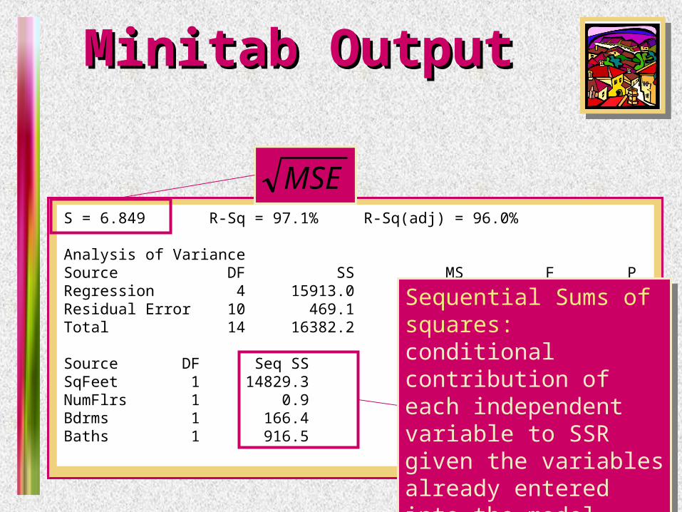
S = 6.849 R-Sq = 97.1% R-Sq(adj) = 96.0%

Analysis of VarianceSource DF SS MS F PRegression 4 15913.0 3978.3 84.80 0.000Residual Error 10 469.1 46.9Total 14 16382.2

Source DF Seq SSSqFeet 1 14829.3NumFlrs 1 0.9Bdrms 1 166.4Baths 1 916.5

MSE

Sequential Sums of squares: conditional contribution of each independent variable to SSR given the variables already entered into the model.

Sequential Sums of squares: conditional contribution of each independent variable to SSR given the variables already entered into the model.

Note 14 of 5E

Minitab OutputMinitab OutputIs the overall model useful in predicting list price? How much of the overall variation in the response is explained by the regression model?S = 6.849 R-Sq = 97.1% R-Sq(adj) = 96.0%

Analysis of VarianceSource DF SS MS F PRegression 4 15913.0 3978.3 84.80 0.000Residual Error 10 469.1 46.9Total 14 16382.2

Source DF Seq SSSqFeet 1 14829.3NumFlrs 1 0.9Bdrms 1 166.4Baths 1 916.5

F = MSR/MSE = 84.80 with p-value = .000 is highly significant. The model is very useful in predicting the list price of homes.

F = MSR/MSE = 84.80 with p-value = .000 is highly significant. The model is very useful in predicting the list price of homes.

R2 = .971 indicates that 97.1% of the overall variation is explained by the regression model.

Note 14 of 5E

Minitab OutputMinitab OutputIn the presence of the other three independent variables, is the number of bedrooms significant in predicting the list price of homes? Test using = .05.

Regression Analysis: ListPrice versus SqFeet, NumFlrs, Bdrms, BathsThe regression equation isListPrice = 18.8 + 6.27 SqFeet - 16.2 NumFlrs - 2.67 Bdrms + 30.3 Baths

Predictor Coef SE Coef T PConstant 18.763 9.207 2.04 0.069SqFeet 6.2698 0.7252 8.65 0.000NumFlrs -16.203 6.212 -2.61 0.026Bdrms -2.673 4.494 -0.59 0.565Baths 30.271 6.849 4.42 0.001

To test H0: the test statistic is t = -0.59 with p-value = .565.

The p-value is larger than .05 and H0 is not rejected.

We cannot conclude that number of bedrooms is a valuable predictor in the presence of the other variables.

Perhaps the model could be refit without x3.

Note 14 of 5E

Historical NoteHistorical Note Where does the name “regression” come

from? In 1886, geneticist Francis Galton set up a

stand at the Great Exhibition, where he measured the heights of families attending. He discovered a phenomenon called “regression toward the mean”. Seeking laws of inheritance, he found that son’s heights tended to regress toward the mean height of the population, compared to their father’s heights. Tall fathers tended to have somewhat shorter sons, and vice versa. Galton developed regression analysis to study this effect, which he optimistically referred to as “regression towards mediocrity".

Note 14 of 5E