Notes for the International Summer School on Advanced ...bme.elektro.dtu.dk/31545/notes/ref_jaj_2015.pdf · Notes for the International Summer School on Advanced Ultrasound Imaging

Notes for the International Summer Schoolon Advanced Ultrasound Imaging

Jørgen Arendt Jensen

May 26, 2015

Center for fast Ultrasound Imaging, Dept. of Elec. Eng., Technical University of Denmark

This page is inserted to facilitate double sided printing.

CONTENTS

1 Introduction 1

2 Description of ultrasound fields 32.1 Fields in linear acoustic systems . . . . . . . . . . . . . . . . . . . . . . . . . . . . . . . . . . . . . 32.2 Basic theory . . . . . . . . . . . . . . . . . . . . . . . . . . . . . . . . . . . . . . . . . . . . . . . 42.3 Calculation of spatial impulse responses . . . . . . . . . . . . . . . . . . . . . . . . . . . . . . . . . 82.4 Apodization and soft baffle . . . . . . . . . . . . . . . . . . . . . . . . . . . . . . . . . . . . . . . . 162.5 Examples of spatial impulse responses . . . . . . . . . . . . . . . . . . . . . . . . . . . . . . . . . 172.6 Calculation of the scattered signal . . . . . . . . . . . . . . . . . . . . . . . . . . . . . . . . . . . . 19

3 Ultrasound imaging 313.1 Fourier relation . . . . . . . . . . . . . . . . . . . . . . . . . . . . . . . . . . . . . . . . . . . . . . 313.2 Focusing . . . . . . . . . . . . . . . . . . . . . . . . . . . . . . . . . . . . . . . . . . . . . . . . . 363.3 Fields from array transducers . . . . . . . . . . . . . . . . . . . . . . . . . . . . . . . . . . . . . . 373.4 Imaging with arrays . . . . . . . . . . . . . . . . . . . . . . . . . . . . . . . . . . . . . . . . . . . 403.5 Simulation of ultrasound imaging . . . . . . . . . . . . . . . . . . . . . . . . . . . . . . . . . . . . 463.6 Synthetic phantoms . . . . . . . . . . . . . . . . . . . . . . . . . . . . . . . . . . . . . . . . . . . 493.7 Anatomic phantoms . . . . . . . . . . . . . . . . . . . . . . . . . . . . . . . . . . . . . . . . . . . 51

4 Ultrasound Velocity Imaging 554.1 Introduction: Blood Velocity Estimation Systems . . . . . . . . . . . . . . . . . . . . . . . . . . . . 564.2 The human circulation . . . . . . . . . . . . . . . . . . . . . . . . . . . . . . . . . . . . . . . . . . 564.3 Ultrasound scattering from blood . . . . . . . . . . . . . . . . . . . . . . . . . . . . . . . . . . . . 564.4 Ultrasound signals from flowing blood . . . . . . . . . . . . . . . . . . . . . . . . . . . . . . . . . 594.5 Simulation of flow signals . . . . . . . . . . . . . . . . . . . . . . . . . . . . . . . . . . . . . . . . 614.6 Estimation of the velocity distribution . . . . . . . . . . . . . . . . . . . . . . . . . . . . . . . . . . 624.7 Axial velocity estimation using the phase . . . . . . . . . . . . . . . . . . . . . . . . . . . . . . . . 634.8 Axial velocity estimation using the time shift . . . . . . . . . . . . . . . . . . . . . . . . . . . . . . 674.9 Two-dimensional vector velocity estimation . . . . . . . . . . . . . . . . . . . . . . . . . . . . . . . 694.10 Three-dimensional vector velocity estimation . . . . . . . . . . . . . . . . . . . . . . . . . . . . . . 724.11 Synthetic aperture and plane wave flow estimation . . . . . . . . . . . . . . . . . . . . . . . . . . . 724.12 Motion estimation and other uses . . . . . . . . . . . . . . . . . . . . . . . . . . . . . . . . . . . . 77

5 Synthetic aperture ultrasound imaging 81

6 Sequential beamforming for synthetic aperture imaging 93

i

ii

CHAPTER

ONE

Introduction

These notes have been prepared for the international summer school on advanced ultrasound imaging in June 2015 atthe Technical University of Denmark. The notes should be read in conjunction with the notes prepared by Trahey1.The intended audience is Ph.D. students working in medical ultrasound. A knowledge of general linear acoustics andsignal processing is assumed.

The notes give a linear description of general ultrasound imaging through the use of spatial impulse responses. It isshown in Chapter 2 how both the emitted and scattered fields for the pulsed and continuous wave case can be calculatedusing this approach. Chapter 3 gives a brief overview of modern ultrasound imaging and how it is simulated usingspatial impulse responses. The first two chapters are based on the previous summer school course notes in [2]. Chapter4 gives a brief description of both spectral and color flow imaging systems and their modeling and simulation alongwith the more modern vector velocity systems. This is based on the book chapter in [3]. A description of syntheticaperture imaging is given in Chapter 5 based on [4]. The final chapter is on sequential beamforming for syntheticaperture imaging and is based on [5].

For the summer school it is assumed that the participant has read and understands the first two chapters on linearimaging. Lectures will be given on the content of the other chapters.

Jørgen Arendt JensenMay, 2015.

Center for fast Ultrasound ImagingDTU Elektro, Build. 349,Technical University of DenmarkDK-2800 Lyngby, DenmarkE-mail: [email protected]: http://bme.elektro.dtu.dk/jaj/

1[1] Martin E. Anderson, Nick Bottenus and Gregg E. Trahey: A seminar on k-space applied to medical ultrasound, Dept. of BiomedicalEngineering, Duke University, 2015

1

http://www.elektro.dtu.dk/cfu

http://www.elektro.dtu.dk/

http://www.dtu.dk/

mailto: [email protected]

http://bme.elektro.dtu.dk/jaj/

2

CHAPTER

TWO

Description of ultrasound fields

This chapter gives a linear description of acoustic fields using spatial impulse responses. It is shown how both thepulsed emitted and scattered fields can be accurately derived using spatial impulse responses, and how attenuation anddifferent boundary conditions can be incorporated. The chapter goes into some detail of deriving the different resultsand explaining their consequence. Different examples for both simulated and measured fields are given. The chapteris based on the papers [6], [7] and [8] and on the book [9].

2.1 Fields in linear acoustic systems

It is a well known fact in electrical engineering that a linear electrical system is fully characterized by its impulse re-sponse as shown in Fig. 2.1. Applying a delta function to the input of the circuit and measuring its output characterizesthe system. The output y(t) to any kind of input signal x(t) is then given by

y(t) = h(t) ∗ x(t) =

∫ +∞

−∞h(θ)x(t− θ)dθ, (2.1)

where h(t) is the impulse response of the linear system and ∗ denotes time convolution. The transfer function of thesystem is given by the Fourier transform of the impulse response and characterizes the systems amplification of atime-harmonic input signal.

The same approach can be taken to characterize a linear acoustic system. The basic set-up is shown in Fig. 2.2. Theacoustic radiator (transducer) on the left is mounted in a infinite rigid, baffle and its position is denoted by ~r2. It radiatesinto a homogeneous medium with a constant speed of sound c and density ρ0 throughout the medium. The pointdenoted by ~r1 is where the acoustic pressure from the transducer is measured by a small point hydrophone. A voltageexcitation of the transducer with a delta function will give rise to a pressure field that is measured by the hydrophone.The measured response is the acoustic impulse response for this particular system with the given set-up. Moving thetransducer or the hydrophone to a new position will give a different response. Moving the hydrophone closer to the

Figure 2.1: Measurement of impulse response for a linear electric system.

3

Figure 2.2: A linear acoustic system.

transducer surface will often increase the signal1, and moving it away from the center axis of the transducer will oftendiminish it. Thus, the impulse response depends on the relative position of both the transmitter and receiver (~r2 − ~r1)and hence it is called a spatial impulse response.

A perception of the sound field for a fixed time instance can be obtained by employing Huygens’ principle in whichevery point on the radiating surface is the origin of an outgoing spherical wave. This is illustrated in Fig. 2.3. Each ofthe outgoing spherical waves are given by

ps(~r1, t) = δ

(t− |~r2 − ~r1|

c

)= δ

(t− |r|

c

)(2.2)

where ~r1 indicates the point in space, ~r2 is the point on the transducer surface, and t is the time for the snapshot of thespatial distribution of the pressure. The spatial impulse response is then found by observing the pressure waves at afixed position in space over time by having all the spherical waves pass the point of observation and summing them.Being on the acoustical axis of the transducer gives a short response whereas an off-axis point yields a longer impulseresponse as shown in Fig. 2.3.

2.2 Basic theory

In this section the exact expression for the spatial impulse response will more formally be derived. The basic setup isshown in Fig. 2.4. The triangularly shaped aperture is placed in an infinite, rigid baffle on which the velocity normalto the plane is zero, except at the aperture. The field point is denoted by ~r1 and the aperture by ~r2. The pressure fieldgenerated by the aperture is then found by the Rayleigh integral [10]

p(~r1, t) =ρ0

2π

∫S

∂vn(~r2, t− |~r1−~r2|c )

∂t| ~r1 − ~r2 |

dS, (2.3)

where vn is the velocity normal to the transducer surface. The integral is a statement of Huyghens’ principle that thefield is found by integrating the contributions from all the infinitesimally small area elements that make up the aperture.This integral formulation assumes linearity and propagation in a homogeneous medium without attenuation. Further,the radiating aperture is assumed flat, so no re-radiation from scattering and reflection takes place. Exchanging theintegration and the partial derivative, the integral can be written as

p(~r1, t) =ρ0

2π

∂

∫S

vn(~r2, t− |~r1−~r2|c )

| ~r1 − ~r2 |dS

∂t. (2.4)

1This is not always the case. It depends on the focusing of the transducer. Moving closer to the transducer but away from its focus will decreasethe signal.

4 Chapter 2. Description of ultrasound fields

Figure 2.3: Illustration of Huygens’ principle for a fixed time instance. A spherical wave with a radius of |~r| = ct isradiated from each point on the aperture.

Figure 2.4: Position of transducer, field point, and coordinate system.

2.2. Basic theory 5

It is convenient to introduce the velocity potential ψ that satisfies the equations [11]

~v(~r, t) = −∇ψ(~r, t)

p(~r, t) = ρ0∂ψ(~r, t)

∂t. (2.5)

Then only a scalar quantity need to be calculated and all field quantities can be derived from it. The surface integral isthen equal to the velocity potential:

ψ(~r1, t) =

∫S

vn(~r2, t− |~r1−~r2|c )

2π | ~r1 − ~r2 |dS (2.6)

The excitation pulse can be separated from the transducer geometry by introducing a time convolution with a deltafunction as

ψ(~r1, t) =

∫S

∫T

vn(~r2, t2)δ(t− t2 − |~r1−~r2|c )

2π | ~r1 − ~r2 |dt2dS, (2.7)

where δ is the Dirac delta function.

Assume now that the surface velocity is uniform over the aperture making it independent of ~r2, then:

ψ(~r1, t) = vn(t) ∗∫S

δ(t− |~r1−~r2|c )

2π | ~r1 − ~r2 |dS, (2.8)

where ∗ denotes convolution in time. The integral in this equation

h(~r1, t) =

∫S

δ(t− |~r1−~r2|c )

2π | ~r1 − ~r2 |dS (2.9)

is called the spatial impulse response and characterizes the three-dimensional extent of the field for a particular trans-ducer geometry. Note that this is a function of the relative position between the aperture and the field.

Using the spatial impulse response the pressure is written as

p(~r1, t) = ρ0∂vn(t)

∂t∗ h(~r1, t) (2.10)

which equals the emitted pulsed pressure for any kind of surface vibration vn(t). The continuous wave field can befound from the Fourier transform of (2.10). The received response for a collection of scatterers can also be foundfrom the spatial impulse response [12], [6]. This is derived in Section 2.6. Thus, the calculation of the spatial impulseresponse makes it possible to find all ultrasound fields of interest.

2.2.1 Geometric considerations

The calculation of the spatial impulse response assumes linearity and any complex-shaped transducer can thereforebe divided into smaller apertures and the response can be found by adding the responses from the sub-apertures. Theintegral is, as mentioned before, a statement of Huyghens’ principle of summing contributions from all areas of theaperture.

An alternative interpretation is found by using the acoustic reciprocity theorem [13]. This states that: ”If in anunchanging environment the locations of a small source and a small receiver are interchanged, the received signal willremain the same.” Thus, the source and receiver can be interchanged. Emitting a spherical wave from the field pointand finding the wave’s intersection with the aperture also yields the spatial impulse response. The situation is depictedin Fig. 2.5, where an outgoing spherical wave is emitted from the origin of the coordinate system. The dashed curvesindicate the circles from the projected spherical wave.

The calculation of the impulse response is then facilitated by projecting the field point onto the plane of the aperture.The task is thereby reduced to a two-dimensional problem and the field point is given as a (x, y) coordinate set and a


x

y

z

Figure 2.5: Emission of a spherical wave from the field point and its intersection of the aperture.

Aperture

Field point

x

y

r1

r2

Figure 2.6: Intersection of spherical waves from the field point by the aperture, when the field point is projected ontothe plane of the aperture.

2.2. Basic theory 7

Figure 2.7: Definition of distances and angles in the aperture plan for evaluating the Rayleigh integral.

height z above the plane. The three-dimensional spherical waves are then reduced to circles in the x − y plane withthe origin at the position of the projected field point as shown in Fig. 2.6.

The spatial impulse response is, thus, determined by the relative length of the part of the arc that intersects the aperture.Thereby it is the crossing of the projected spherical waves with the edges of the aperture that determines the spatialimpulse responses. This fact is used for deriving equations for the spatial impulse responses in the next section.

2.3 Calculation of spatial impulse responses

The spatial impulse response is found from the Rayleigh integral derived earlier

h(~r1, t) =

∫S

δ(t− |~r1−~r2|c )

2π | ~r1 − ~r2 |dS (2.11)

The task is to project the field point onto the plane coinciding with the aperture, and then find the intersection of theprojected spherical wave (the circle) with the active aperture as shown in Fig. 2.6.

Rewriting the integral into polar coordinates gives:

h(~r1, t) =

∫ Θ2

Θ1

∫ d2

d1

δ(t− Rc )

2πRr dr dΘ (2.12)

where r is the radius of the projected circle and R is the distance from the field point to the aperture given by R2 =r2 + z2

p . Here zp is the field point height above the x − y plane of the aperture. The projected distances d1, d2 aredetermined by the aperture and are the distance closest to and furthest away from the aperture, and Θ1,Θ2 are thecorresponding angles for a given time (see Fig. 2.7).

Introducing the substitution 2RdR = 2rdr gives

h(~r1, t) =1

2π

∫ Θ2

Θ1

∫ R2

R1

δ(t− R

c) dR dΘ (2.13)


The variables R1 and R2 denote the edges closest to and furthest away from the field point. Finally using the substi-tution t′ = R/c gives

h(~r1, t) =c

2π

∫ Θ2

Θ1

∫ t2

t1

δ(t− t′)dt′dΘ (2.14)

For a given time instance the contribution along the arc is constant and the integral gives

h(~r1, t) =Θ2 −Θ1

2πc (2.15)

when assuming the circle arc is only intersected once by the aperture. The angles Θ1 and Θ2 are determined bythe intersection of the aperture and the projected spherical wave, and the spatial impulse response is, thus, solelydetermined by these intersections, when no apodization of the aperture is used. The response can therefore be evaluatedby keeping track of the intersections as a function of time.

2.3.1 A simple calculation procedure

From the derivation in the last section it can be seen that the spatial impulse response in general can be expressed as

h(~r1, t) =c

2π

N(t)∑i=1

[Θ

(i)2 (t)−Θ

(i)1 (t)

](2.16)

whereN(t) is the number of arc segments that crosses the boundary of the aperture for a given time and Θ(i)2 (t),Θ

(i)1 (t)

are the associated angles of the arc. This was also noted by Stepanishen [14]. The calculation can, thus, be formulatedas finding the angles of the aperture edge’s intersections with the projected spherical wave, sorting the angles, andthen summing the arc angles that belong to the aperture. Finding the intersections can be done from the descriptionof the edges of the aperture. A triangle can be described by three lines, a rectangle by four, and the intersections arethen found from the intersections of the circle with the lines. This makes it possible to devise a general procedure forcalculating spatial impulse responses for any flat, bounded aperture, since the task is just to find the intersections ofthe boundary with the circle.

The spatial impulse response is calculated from the time the aperture first is intersected by a spherical wave to the timefor the intersection furthest away. The intersections are found for every time instance and the corresponding anglesare sorted. The angles lie in the interval from 0 to 2π. It is then found whether the arc between two angles belongsto the aperture, and the angle difference is added to the sum, if the arc segment is inside the aperture. This yields thespatial impulse response according to Eq. (2.16). The approach can be described by the flow chart shown in Fig. 2.8.

The only part of the algorithm specific to the aperture is the determination of the intersections and whether the pointis inside the aperture. Section 2.3.2 shows how this is done for polygons, Section 2.3.3 for circles, and Section 2.3.6for higher-order parametric boundaries.

All the intersections need not be found for all times. New intersections are only introduced, when a new edge or cornerof the aperture is met. Between times when two such corners or edges are encountered the number of intersectionsremains constant and only intersections, which belong to points inside the aperture need to be found. Note that anaperture edge gives rise to a discontinuity in the spatial impulse response. Also testing whether the point is inside theaperture is often superfluous, since this only needs to be found once after each discontinuity in the response. These twoobservations can significantly reduce the number of calculations, since only the intersections affecting the responseare found.

The procedure first finds the number of discontinuities. Then only intersection influencing the response are calculatedbetween two discontinuity points. This can potentially make the approach faster than the traditional approach, wherethe response from a number of different rectangles or triangles must be calculated.

2.3. Calculation of spatial impulse responses 9

Figure 2.8: Flow chart for calculating the spatial impulse response.


Figure 2.9: Definition of bounding lines for polygon transducer. The arrows indicate the half-planes for the activeaperture.

2.3.2 Solution for polygons

The boundary of any polygon can be defined by a set of bounding lines as shown in Fig. 2.9.

The active aperture is then defined as lying on one side of the line as indicated by the arrows, and a point on theaperture must be placed correctly in relation to all lines. The test whether a point is on the aperture is thus to gothrough all lines and test whether the point lies in the active half space for the line, and stop if it is not. The point isinside the aperture, if it passes the test for all the lines.

The intersections are found from the individual intersections between the projected circle and the lines. They aredetermined from the equations for the projected spherical wave and the line:

r2 = (x− x0)2 + (y − y0)2

y = αx+ y1 (2.17)r2 = (ct)2 − z2

p

Here (x0, y0) is the center of the circle, α the slope of the line, and y1 its intersect with the y-axis. The intersectionsare given from the solutions to:

0 = (1 + α2)x2 + (2αy1 − 2x0 − 2y0α)x+ (y20 + y2

1 + x20 − 2y0y1 − r2)

= Ax2 +Bx+ C (2.18)D = B2 − 4AC

The angles are

Θ = arctan

(y − y0

x− x0

)(2.19)

Intersections between the line and the circle are only found if D > 0. A determinant D < 0 indicates that the circledid not intersect the line. If the line has infinite slope, the solution is found from the equation:

x = x1

0 = y2 − 2y0y + y20 + (x1 − x0)2 − r2 (2.20)

= A∞y2 +B∞y + C∞

in which A∞, B∞, C∞ replace A,B,C, respectively, and the solutions are found for y rather than x. Here x1 is theline’s intersection with the x-axis.

The times for discontinuities in the spatial impulse response are given by the intersections of the lines that define theaperture’s edges and by the minimum distance from the projected field point to the lines. The minimum distance is


found from a line passing through the field point that is orthogonal to the bounding line. The intersection between theorthogonal line and the bounding line is:

x =αyp + xp − αy1

α2 + 1(2.21)

y = αx+ y1

where (xp, yp, zp) is the position of the field point. For an infinite slope line the solution is x = x1 and y = yp. Thecorresponding time is:

ti =

√(x− xp)2 + (y − yp)2 + z2

p

c(2.22)

The intersections of the lines are also found, and the corresponding times are calculated by (2.22) and sorted inascending order. They indicate the start and end time for the response and the time points for discontinuities in theresponse.

2.3.3 Solution for circular surfaces

The other basic shape for a transducer apart from rectangular shapes is the flat, round surface used for single elementpiston transducers and annular arrays. For these the intersections are determined by two circles as depicted in Fig. 2.10.

Here O1 is the center of the aperture with radius ra and the projected spherical wave is centered at O2 with radiusrb(t) =

√(ct)2 − z2

p . The length ha(t) is given by [15, page 66]

ha(t) =2√p(t)(p(t)− a)(p(t)− ra)(p(t)− rb(t))

a(2.23)

a = ||O1 −O2||

p(t) =a+ ra + rb(t)

2

In a coordinate system centered at O1 and an x-axis in the O1 −O2 direction, the intersections are at

y = ha(t) (2.24)

l = ±√r2b (t)− h2

a(t)

The sign for l depends on the position of the intersections. A negative sign is used if the intersections are for negativevalues of x, and positive sign is used for positive x positions.

When the field point is outside the active aperture the spatial impulse response is

h(~r1, t) =|Θ2 −Θ1|

2πc =

c

πarctan

(ha(t)

l

)(2.25)

Θ2 = arctan

(ha(t)

l

)= −Θ1

It must be noted that a proper four-quadrant arc-tan should be used to give the correct response. An alternative formulais [16, page 19]

h(~r1, t) =c

2πarcsin

(2√p(t)(p(t)− a)(p(t)− ra)(p(t)− rb(t))

r2b (t)

)(2.26)

=c

2πarcsin

(aha(t)

r2b (t)

)


Figure 2.10: Geometry for determining intersections between circles. The top graph shows the geometry when thefield point denoted by O2 is outside the aperture, and the bottom graph when it is inside.


The start time ts for the response is found from

ra + rb(t) = ||O1 −O2||

ts =

√r2b (t) + z2

p

c=

√(||O1 −O2|| − ra)2 + z2

p

c(2.27)

and the response ends at the time te when

rb(t) = ra + ||O1 −O2||

te =

√r2b (t) + z2

p

c=

√(||O1 −O2||+ ra)2 + z2

p

c(2.28)

When the field point is inside the aperture, the response is

h(~r1, t) = c forzpc≤ t ≤

√(ra − ||O1 −O2||)2 + z2

p

c(2.29)

thereafter the arc lying outside the aperture should be subtracted, so that

h(~r1, t) =2π − |Θ2 −Θ1|

2πc (2.30)

The response ends when

rb(t) = ra + ||O1 −O2||

te =

√(||O1 −O2||+ ra)2 + z2

p

c(2.31)

The determination of which part of the arc that subtracts or adds to the response is determined by what the activeaperture is. One ring in an annular array can be defined as consisting of an active aperture outside a circle combinedwith an active aperture inside a circle for defining the inner and outer rim of the aperture. A circular aperture can alsobe combined with a line for defining the active area of a split aperture used for continuous wave probing.

2.3.4 Solution for a circular concave surface

For reference the expression for a concave transducer, which is a type often used in medical ultrasonics, is given. Aderivation of the solution can be found in [17] and [18].

The spatial impulse response is [17]:

hc(~r1, t) =

Region I Region IIz < 0 z > 0

0 ct < r0 r0 < ct ct < r1cRr r0 < ct < r1 r2 < ct < r0 −cRr

1π arccos η(t)

σ(t) r1 < ct < r2 r1 < ct < r2 r1 < ct < r2

0 r2 < ct ct < r1 r2 < ct

(2.32)

where:

η(t) = R

{1− d/R

sin Θ+

1

tan Θ

(R2 + r2 − c2t2

2rR

)}

σ(t) = R

√1−

(R2 + r2 − c2t2

2rR

)2

(2.33)

r = |~r1 |.

The variables are defined in Fig. 2.11.


x

z

r1

d

r2

r0

r1

R

Θ

Aperture

Field point

Region I

Region II

x

z

r1

dr2

r0

r1

R

Θ

Aperture

Field point

Figure 2.11: Definition of variables for spatial impulse response of concave transducer.


2.3.5 Solution for other surfaces

Analytical solutions for spatial impulse response have been derived for a number of different geometries by variousauthors. The response from a flat rectangle can be found in [19, 20], and for a flat triangle in [21]).

2.3.6 Solution for parametric surfaces

For ellipses or other higher order parametric surfaces it is in general not easy to find analytic solutions for the spatialimpulse response. The boundary method described above can, however, be used for providing a simple solution to theproblem, since the intersections between the projected spherical wave and the edge of the aperture uniquely determinethe spatial impulse response. It is therefore possible to use root finding for a set of (non-linear) equations for findingthese intersections. The problem is to find when both the spherical wave and the aperture have crossing contours inthe plane of the aperture, i.e., when

(ct)2 − z2p − (x− xp)2 − (y − yp)2 = 0 (2.34)

S(x, y) = 0

in which S(x, y) = 0 defines the boundary of the aperture. The problem of numerically finding these roots is ingeneral not easy, if a good initial guess on the position of the intersections is not found [22, pages 286–289]. Goodinitial values are however found here, since the intersections must lie on the projected circle and the intersections onlymove slightly from time point to time point. An efficient Newton-Raphson algorithm can therefore be devised forfinding the intersections, and the procedure detailed here can be used to find the spatial impulse response for any flattransducer geometry with an arbitrary apodization and both hard and soft baffle mounting.

2.4 Apodization and soft baffle

Often ultrasound transducers do not vibrate as a piston over the aperture. This can be due to the clamping of the activesurface at its edges, or intentionally to reduce side-lobes in the field. Applying for example a Gaussian apodizationwill significantly lower side lobes and generate a field with a more uniform point spread function as a function ofdepth. Apodization is introduced in (2.12) by writing [23]

h(~r1, t) =

∫ Θ2

Θ1

∫ d2

d1

ap(r,Θ)δ(t− R

c )

2πRr dr dΘ (2.35)

in which ap(r,Θ) is the apodization over the aperture. Using the same substitutions as before yields

h(~r1, t) =c

2π

∫ Θ2

Θ1

∫ t2

t1

ap1(t′,Θ)δ(t− t′) dt′ dΘ (2.36)

where ap1(t′,Θ) = ap(√

(ct′)2 − z2p,Θ). The inner integral is a convolution of the apodization function with a

δ-function and readily yields

h(~r1, t) =c

2π

∫ Θ2

Θ1

ap1(t,Θ) dΘ (2.37)

as noted by several authors [23, 24, 25]. The response for a given time instance can, thus, be found by integrating theapodization function along the fixed arc with a radius of r =

√(ct)2 − z2

p for the angles for the active aperture. Anyapodization function can therefore be incorporated into the calculation by employing numerical integration.

Often the assumption of an infinite rigid baffle for the transducer mounting is not appropriate and another form of theRayleigh integral must be used. For a soft baffle, in which the pressure on the baffle surface is zero, the Rayleigh-Sommerfeld integral is used. This is [26, pages 46–50]

hs(~r1, t) =

∫S

δ(t− |~r1−~r2|c )

2π | ~r1 − ~r2 |cosϕ dS (2.38)


Figure 2.12: Definition of angle used for a soft baffle.

assuming that |~r1−~r2| � λ. Here cosϕ is the angle between the line through the field point orthogonal to the apertureplane and the radius of the spherical wave as shown in Fig. 2.12.

The angle ϕ is constant for a given radius of the projected spherical wave and thus for a given time. It is given by

cosϕ =zpR

=zpct

(2.39)

Using the substitutions from Section 2.2, the Rayleigh-Sommerfeld integral can then be rewritten as

hs(~r1, t) =zp2πc(Θ2 −Θ1)

∫ t2

t1

δ(t− t′)ct′

dt′ (2.40)

Using the property of the δ-function that ∫ +∞

−∞g(t′)δ(t− t′) dt′ = g(t) (2.41)

then gives

hs(~r1, t) =zpct

Θ2 −Θ1

2πc =

zpcth(~r1, t). (2.42)

The spatial impulse response can, thus, be found from the spatial impulse response for the rigid baffle case by multi-plying with zp/(ct).

2.5 Examples of spatial impulse responses

The first example shows the spatial impulse responses from a 3× 5 mm rectangle for different spatial positions 5 mmfrom the front face of the transducer. The responses are found from the center of the rectangle (y = 0) and out in stepsof 2 mm in the x direction to 6 mm away from the center of the rectangle. A schematic diagram of the situation isshown in Fig. 2.13 for the on-axis response. The impulse response is zero before the first spherical wave reaches theaperture. Then the response stays constant at a value of c. The first edge of the aperture is met, and the response drops

2.5. Examples of spatial impulse responses 17

x

y

h

t

Aperture

Spherical waves

Figure 2.13: Schematic diagram of field from rectangular element.

33.5

44.5

55.5

6x 10

−6 0

1

2

3

4

5

6

0

200

400

600

800

1000

1200

1400

1600

Lateral distance [mm]

Time [s]

h [

m/s

]

Figure 2.14: Spatial impulse response from a rectangular aperture of 4× 5 mm at for different lateral positions


of. The decrease with time in increased when the next edge of the aperture is reached and the response becomes zerowhen the projected spherical waves all are outside the area of the aperture.

A plot of the results for the different lateral field positions is shown in Fig. 2.14. It can be seen how the spatial impulseresponse changes as a function of relative position to the aperture.

The second example shows the response from a circular, flat transducer. Two different cases are shown in Fig. 2.15.The top graph shows the traditional spatial impulse response when no apodization is used, so that the aperture vibratesas a piston. The field is calculated 10 mm from the front face of the transducer starting at the center axis of the aperture.Twenty-one responses for lateral distance of 0 to 20 mm off axis are then shown. The same calculation is repeated inthe bottom graph, when a Gaussian apodization has been imposed on the aperture. The vibration amplitude is a factorof 1/ exp(4) less at the edges of the aperture than at the center. It is seen how the apodization reduces some of thesharp discontinuities in the spatial impulse response, which can reduce the sidelobes of the field.

2.6 Calculation of the scattered signal

In medical ultrasound, a pulsed field is emitted into the body and is scattered and reflected by density and propagationvelocity perturbations. The scattered field then propagates back through the tissue and is received by the transducer.The field is converted to a voltage signal and used for the display of the ultrasound image. A full description of atypical imaging system, using the concept of spatial impulse response, is the purpose of the section.

The received signal can be found by solving an appropriate wave equation. This has been done in a number of papers(e.g. [27], [28]). Gore and Leeman [27] considered a wave equation where the scattering term was a function ofthe adiabatic compressibility and the density. The transducer was modeled by an axial and lateral pulse that wereseparable. Fatemi and Kak [28] used a wave equation where scattering originated only from velocity fluctuations, andthe transducer was restricted to be circularly symmetric and unfocused (flat).

The scattering term for the wave equation used here is a function of density and propagation velocity perturbations,and the wave equation is equivalent to the one used by Gore and Leeman [27]. No restrictions are enforced on thetransducer geometry or its excitation, and analytic expressions for a number of geometries can be incorporated intothe model.

The model includes attenuation due to propagation and scattering, but not the dispersive attenuation observed forpropagation in tissue. This can, however, be incorporated into the model as indicated in Section 2.6.6.

The derivation is organized as follows. The following section derives the wave equation and describes the differentlinearity assumptions made. Section 2.6.2 calculates the scattered field and section 2.6.3 introduces the spatial impulseresponse model for the incident field. Section 2.6.4 combines the wave equation solution and the transducer model togive the final equation for the received pressure field. To indicate the precision of the model, a single example of apredicted pressure field compared to measured field is given in Section 2.6.5.

2.6.1 Derivation of the wave equation

This section derives the wave equation. The section has been included in order to explain in detail the differentlinearity assumptions and approximations made to obtain a solvable wave equation. The derivation closely followsthat developed by Chernov (1960).

The first approximation states that the instantaneous acoustic pressure and density can be written

Pins(~r, t) = P + p1(~r, t) (2.43)ρins(~r, t) = ρ(~r) + ρ1(~r, t) (2.44)

in which P is the mean pressure of the medium and ρ is the density of the undisturbed medium. Here p1 is the pressure

2.6. Calculation of the scattered signal 19

0.60.8

11.2

1.41.6

1.8

x 10−5

0

5

10

15

20

0

200

400

600

800

1000

1200

1400

1600


Response from circular, non−apodized transducer

Time [s]

h [

m/s

]

0.60.8

11.2

1.41.6

1.8

x 10−5

0

5

10

15

20

0

200

400

600

800

1000

1200

1400

1600


Response from circular, Gaussian apodized transducer

Time [s]

h [

m/s

]

Figure 2.15: Spatial impulse response from a circular aperture. Graphs are shown without apodization of the aperture(top) and with a Gaussian apodization function (bottom). The radius of the aperture is 5 mm and the field is calculated10 mm from the transducer surface.


variation caused by the ultrasound wave and is considered small compared to P and ρ1 is the density change causedby the wave. Both p1 and ρ1 are small quantities of first order.

Our second assumption is that no heat conduction or conversion of ultrasound to thermal energy take place. Thus, theentropy is constant for the process, so that the acoustic pressure and density satisfy the adiabatic equation [29]:

dPinsdt

= c2dρinsdt

(2.45)

The equation contains total derivatives, as the relation is satisfied for a given particle of the tissue rather than at agiven point in space. This is the Lagrange description of the motion [11]. For our purpose the Euler description ismore appropriate. Here the coordinate system is fixed in space and the equation describes the properties of whateverparticle of fluid there is at a given point at a given time. Converting to an Eulerian description results in the followingconstitutive equation [29], [11]:

1

c2∂p1

∂t=∂ρ1

∂t+ ~u · ∇ρ (2.46)

using that P and ρ do not depend on time and that ρ1 is small compared to ρ. Here u is the particle velocity, ∇ is thegradient operator, and · symbolizes the scalar product.

The pressure, density, and particle velocity must also satisfy the hydrodynamic equations [29]:

ρinsd~u

dt= −∇Pins (2.47)

∂ρins∂t

= −∇ · (ρins~u) (2.48)

which are the dynamic equation and the equation of continuity. Using (2.43) and (2.44) and discarding higher orderterms we can write

ρ∂~u

∂t= −∇p1 (2.49)

∂ρ1

∂t= −∇ · (ρ~u) (2.50)

Differentiating (2.50) with respect to t and inserting (2.49) gives

∂2ρ1

∂2t= −∇ · (ρ∂~u

∂t) = −∇ · (−∇p1) = ∇2p1 (2.51)

Differentiating (2.46) with respect to t1

c2∂2p1

∂2t=∂2ρ1

∂2t+∂~u

∂t· ∇ρ (2.52)

and inserting (2.51) and (2.49) leads to

∇2p1 −1

c2∂2p1

∂2t=

1

ρ∇ρ · ∇p1 (2.53)

Assuming that the propagation velocity and the density only vary slightly from their mean values yields

ρ(~r) = ρ0 + ∆ρ(~r)

c(~r) = c0 + ∆c(~r) (2.54)

where ρ0 � ∆ρ and c0 � ∆c.

∇2p1 −1

(c0 + ∆c)2

∂2p1

∂2t=

1

(ρ0 + ∆ρ)∇(ρ0 + ∆ρ) · ∇p1 (2.55)


Figure 2.16: Coordinate system for calculating the scattered field

Ignoring small quantities of second order and using the approximation (∆� 1):

1

1 + ∆≈ 1−∆ (2.56)

gives:

∇2p1 − (1

c02− 2∆c

c03)∂2p1

∂2t=

(1

ρ0∇(∆ρ)− ∆ρ

ρ02∇(∆ρ)

)· ∇p1 (2.57)

Neglecting the second order term (∆ρ/ρ02)∇(∆ρ) · ∇p1 yields the wave equation:

∇2p1 −1

c20

∂2p1

∂t2= −2∆c

c30

∂2p1

∂t2+

1

ρ0∇(∆ρ) · ∇p1 (2.58)

The two terms on the right side of the equation are the scattering terms which vanish for a homogeneous medium. Thewave equation was derived by Chernov [29]. It has also been considered in Gore & Leeman [27] and Morse & Ingard[11] in a slightly different form, where the scattering terms were a function of the adiabatic compressibility κ and thedensity.

2.6.2 Calculation of the scattered field

Having derived a suitable wave equation, we now calculate the scattered field from a small inhomogeneity embeddedin a homogeneous surrounding. The scene is depicted in Fig. 2.16. The inhomogeneity is identified by ~r1 and enclosedin the volume V ′. The scattered field is calculated at the point indicated by ~r2 by integrating all the spherical wavesemanating from the scattering region V ′ using the time dependent Green’s function for unbounded space. Thus, thescattered field is [11], [27]:

ps(~r2, t) =

∫V ′

∫T

[1

ρ0∇(∆ρ(~r1)) · ∇p1(~r1, t1)

− 2∆c(~r1)

c30

∂2p1(~r1, t1)

∂t2

]G(~r1, t1 | ~r2, t)dt1 d

3~r1 (2.59)

where G is the free space Green’s function:

G(~r1, t1 | ~r2, t) =δ(t− t1 − |~r2−~r1|c0

)

4π | ~r2 − ~r1 |(2.60)


d3~r1 means integrating w.r.t. ~r1 over the volume V ′, and T denotes integration over time.

We denote by

Fop =1

ρ0∇(∆ρ(~r1)) · ∇ − 2∆c(~r1)

c30

∂2

∂t2(2.61)

the scattering operator.

The pressure field inside the scattering region is:

p1(~r, t) = pi(~r, t) + ps(~r, t) (2.62)

where pi is the incident pressure field. As can be seen, the integral can not be solved directly. To solve it we applythe Born-Neumann expansion [30]. If Gi symbolizes the integral operator representing Green’s function and theintegration and Fop the scattering operator, then the first order Born approximation can be written:

ps1(~r2, t) = GiFop pi(~r1, t1) (2.63)

Here ps has been set to zero in (2.62). Inserting ps1 in (2.62) and then in (2.59) we arrive at

ps2(~r2, t) = GiFop [pi(~r1, t1) +GiFop pi(~r1, t1)]

= GiFop pi(~r1, t1) + [GiFop]2pi(~r1, t1) (2.64)

It is emphasized here that Gi indicates an integral over ~r1 and t1, and not the pressure at point ~r1 and time t1 but overthe volume of V ′ and time T indicated by ~r1 and t1.

The general expression for the scattered field then is:

ps(~r2, t) = GiFop pi(~r1, t1) + (2.65)

[GiFop]2pi(~r1, t1) +

[GiFop]3pi(~r1, t1) +

[GiFop]4pi(~r1, t1) + · · ·

Terms involving [GiFop]Npi(~r1, t1), where N > 1, describe multiple scattering of order N . Usually the scattering

from small obstacles is considered weak so higher order terms can be neglected. Thus, a useful approximation is toemploy only the first term in the expansion. This corresponds to the first order Born-approximation.

Using this (2.59) can be approximated by (note the replacement of p1(~r1, t1) with pi(~r1, t1)):

ps(~r2, t) ≈∫V ′

∫T

[1

ρ0∇(∆ρ(~r1)) · ∇pi(~r1, t1)

− 2∆c(~r1)

c30

∂2pi(~r1, t1)

∂t2

]G(~r1, t1 | ~r2, t)dt1 d

3~r1 (2.66)

So in order to calculate the scattered field, the incident field for the homogeneous medium must be calculated.

2.6.3 Calculation of the incident field

The incident field is generated by the ultrasound transducer assuming no other sources exist in the tissue. The fieldis conveniently calculated by employing the velocity potential ψ(~r, t), and enforcing appropriate boundary conditions[31], [32]. The velocity potential satisfies the following wave equation for the homogeneous medium:

∇2ψ − 1

c02

∂2ψ

∂2t= 0 (2.67)


Figure 2.17: Coordinate system for calculating the incident field.

and the pressure is calculated from:

p(~r, t) = ρ0∂ψ(~r, t)

∂t(2.68)

The coordinate system shown in Fig. 2.17 is used in the calculation. The particle velocity normal to the transducersurface is denoted by v(~r3 + ~r4, t), where ~r3 identifies the position of the transducer and ~r4 a point on the transducersurface relative to ~r3.

The solution to the homogeneous wave equation is [32]:

ψ(~r1 + ~r3, t) =

∫S

∫T

v(~r3 + ~r4, t3)g(~r1, t | ~r3 + ~r4, t3)dt3 d2~r4 (2.69)

when the transducer is mounted in a rigid infinite planar baffle. S denotes the transducer surface.

g is the Green’s function for a bounded medium and is

g(~r1, t | ~r3 + ~r4, t3) =δ(t− t3 − |~r1−~r3−~r4|c0

)

2π | ~r1 − ~r3 − ~r4 |(2.70)

| ~r1 − ~r3 − ~r4 | is the distance from S to the point where the field is calculated and c0 the mean propagation velocity.The field is calculated under the assumption of radiation into an isotropic, homogeneous, non-dissipative medium.

If a slightly curved transducer is used, an additional term is introduced as shown in Morse & Feshbach [33]. Thisterm is called the second order diffraction term in Penttinen & Luukkala [18]. It can be shown to vanish for a planartransducer, and as long as the transducer is only slightly curved and large compared to the wavelength of the ultrasound,the resulting expression is a good approximation to the pressure field [18].

If the particle velocity is assumed to be uniform over the surface of the transducer, (2.69) can be reduced to [34]:

ψ(~r1, ~r3, t) =

∫T

v(t3)

∫S

g(~r1, t | ~r3 + ~r4, t3)d2~r4 dt3 (2.71)


Figure 2.18: Coordinate system for calculating the received signal.

This is the spatial impulse response previously derived, and the sound pressure for the incident field then is:

p(~r1, ~r3, t) = ρ0∂ψ(~r1, ~r3, t)

∂t= ρ0v(t) ?

t

∂h(~r1, ~r3, t)

∂t(2.72)

or

p(~r1, ~r3, t) = ρ0∂v(t)

∂t?th(~r1, ~r3, t) (2.73)

2.6.4 Calculation of the received signal

The received signal is the scattered pressure field integrated over the transducer surface, convolved with the electro-mechanical impulse response, Em(t), of the transducer. To calculate this we introduce the coordinate system shownin Fig. 2.18. ~r6 + ~r5 indicates a receiving element on the surface of the transducer that is located at ~r5. The receivedsignal is:

pr(~r5, t) = Em(t) ?t

∫S

ps(~r6 + ~r5, t)d2~r6 (2.74)

The scattered field is:

ps(~r6 + ~r5, t) = 12

∫V ′

∫T

Fop [pi(~r1, t1)]δ(t− t1 − |~r6+~r5−~r1|

c0)

2π | ~r6 + ~r5 − ~r1 |dt1 d

3~r1 (2.75)

Combining this with (2.74) and comparing with (2.9) we see that pr includes Green’s function for bounded spaceintegrated over the transducer surface, which is equal to the spatial impulse response. Inserting the expression for piand performing the integration over the transducer surface and over time, results in:

pr(~r5, t) = Em(t) ?t

12

∫V ′Fop

[ρ0∂v(t)

∂t?th(~r1, ~r3, t)

]?th(~r5, ~r1, t)d

3~r1 (2.76)

If the position of the transmitting and the receiving transducer is the same (~r3 = ~r5), then a simple rearrangement of(2.76) yields:

pr(~r5, t) =ρ0

2Em(t) ?

t

∂v(t)

∂t?t

∫V ′Fop [hpe(~r1, ~r5, t)] d

3~r1 (2.77)


wherehpe(~r1, ~r5, t) = h(~r1, ~r5, t) ?

th(~r5, ~r1, t) (2.78)

is the pulse-echo spatial impulse response.

The calculated signal is the response measured for one given position of the transducer. For a B-mode scan picturea number of scan-lines is measured and combined to a picture. To analyze this situation, the last factor in (2.77) isexplicitly written out ∫

V ′

[1

ρ0∇(∆ρ(~r1)) · ∇hpe(~r1, ~r5, t)−

2∆c(~r1)

c30

∂2hpe(~r1, ~r5, t)

∂t2

]d3~r1 (2.79)

From section 2.6.3 it is know that Hpe is a function of the distance between ~r1 and ~r5, while ∆ρ and ∆c only arefunctions of ~r1. So when ~r5 is varied over the volume of interest, the resulting image is a spatial non-stationaryconvolution between ∆ρ, ∆c and a modified form of the pulse-echo spatial impulse response.

If we assume that the pulse-echo spatial impulse is slowly varying so that the spatial frequency content is constantover a finite volume, then (2.79) can be rewritten∫

V ′

[1

ρ0∆ρ(~r1)∇2hpe(~r1, ~r5, t)−

2∆c(~r1)

c30

∂2hpe(~r1, ~r5, t)

∂t2

]d3~r1 (2.80)

hpe is a function of the distance between the transducer and the scatterer or equivalently of the corresponding timegiven by

t =| ~r1 − ~r5 |

c0(2.81)

The Laplace operator is the second derivative w.r.t. the distance, which can be approximated with the second derivativew.r.t. time. So

∇2hpe(~r1, ~r5, t) =1

c20

∂2hpe(~r1, ~r5, t)

∂t2(2.82)

assuming only small deviations from the mean propagation velocity.

Using these approximations, (2.77) can be rewritten:

pr(~r5, t) =ρ0

2c20Em(t) ?

t

∂v3(t)

∂t3?t

∫V ′

[∆ρ(~r1)

ρ0− 2∆c(~r1)

c0

]hpe(~r1, ~r5, t)d

3~r1 (2.83)

Symbolically this is writtenpr(~r5, t) = vpe(t) ?

tfm(~r1) ?

rhpe(~r1, ~r5, t) (2.84)

?r denotes spatial convolution. vpe is the pulse-echo wavelet which includes the transducer excitation and the electro-

mechanical impulse response during emission and reception of the pulse. fm accounts for the inhomogeneities in thetissue due to density and propagation velocity perturbations which give rise to the scattered signal. hpe is the modifiedpulse-echo spatial impulse response that relates the transducer geometry to the spatial extent of the scattered field.Explicitly written out these terms are:

vpe(t) =ρ0

2c20Em(t) ?

t

∂v3(t)

∂t3(2.85)

fm(~r1) =∆ρ(~r1)

ρ0− 2∆c(~r1)

c0(2.86)

hpe(~r1, ~r5, t) = h(~r1, ~r5, t) ?th(~r5, ~r1, t) (2.87)


−10 −8 −6 −4 −2 0 2 4 6 8 10

7.8

7.9

8

8.1

8.2x 10

−5

x [mm]

Tim

e [

s]

Measured response

−10 −8 −6 −4 −2 0 2 4 6 8 10

7.8

7.9

8

8.1

8.2x 10

−5

x [mm]

Tim

e [

s]

Simulated response

Figure 2.19: Measured and simulated pulse-echo response for a concave transducer. The axial distance was 60 mmand the small scatterer was moved in the lateral direction. The envelope of the RF signal is shown as 6 dB contours.

Expression (2.84) consists of three distinct terms. The interesting signal, and the one that should be displayed inmedical ultrasound, is fm(~r1). We, however, measure a time and spatially smoothed version of this, which obscuresthe finer details in the picture. The smoothing consists of a convolution in time with a fixed wavelet vpe(t) and aspatial convolution with a spatially varying hpe(~r1, ~r5, t).

2.6.5 Example of pulse echo response

To show that the pulse-echo response can be calculated to good accuracy, a single example is shown in Fig. 2.19 for aconcave transducer (r = 8.1 mm) with a focus at R = 150 mm. The measured and simulated responses were obtainedat a distance of 60 mm from the transducer surface. The measured pressure field was acquired by moving a needlepointing toward the transducer in steps of 0.2 mm in the lateral direction, making measurements in a plane containingthe acoustical axis of the transducer. The simulated field was calculated by measuring vpe as the response from aplanar reflector, and then using (2.32) and (2.84) to calculate the field. The envelope of the RF-signals is shown asa contour plot with 6 dB between the contours. The plots span 20 mm in the lateral direction and 4 µs in the axialdirection.

2.6.6 Attenuation effects

The model includes attenuation of the pulse due to propagation, but not the dispersive attenuation of the wave observedwhen propagating in tissue. This changes the pulse continuously as it propagates down through the tissue. Notincluding dispersive attenuation is, however, not a serious drawback of the theory, as this change of the pulse canbe lumped into the already spatially varying hpe. Or, if in the far field and assuming a homogeneous, dispersive


attenuation, then an attenuation transfer function can be convolved onto vpe to yield an attenuated pulse.

Submerging the transducer into a homogeneously attenuating medium will modify the propagation of the sphericalwaves, which will change continuously as a function of distance from the transducer. The spatial impulse is thenchanged to

hatt(t, ~r) =

∫T

∫S

a(t− τ, |~r + ~r1|)δ(τ − |~r+~r1|c )

|~r + ~r1|dSdτ (2.88)

when linear propagation is assumed and the attenuation is the same throughout the medium. a is the attenuationimpulse response. The spherical wave is convolved with the distance dependent attenuation impulse response andspherical waves emanating from different parts of the aperture are convolved with different attenuation impulse re-sponses.

A model for the attenuation must be introduced in order to solve the integral. Ultrasound propagating in tissue ex-periences a nearly linear with frequency attenuation and a commonly used attenuation amplitude transfer functionis

|A′(f, |~r|)| = exp(−β′f |~r|) (2.89)

where β′ is attenuation in nepers per meter. We here prefer to split the attenuation into a frequency dependent and afrequency independent part term as

|A(f, |~r|)| = exp(−α|~r|) exp(−β(f − f0)|~r|) (2.90)

α is the frequency independent attenuation coefficient, and f0 the transducer center frequency. The phase of theattenuation need also be considered. Kak and Dines [35] introduced a linear with frequency phase response

Θ(f) = 2πfτb|~r| (2.91)

where τb is the bulk propagation delay per unit length and is equal to 1/c. This, however, results in an attenuationimpulse response that is non-causal. Gurumurthy and Arthur [36] therefore suggested using a minimum phase impulseresponse, where the amplitude and phase spectrum form a Hilbert transform pair. The attenuation spectrum is thengiven by

A(f, |~r|) = exp(−α|~r|) exp(−β(f − f0)|~r|) (2.92)

× exp(−j2πf(τb + τmβ

π2)|~r|)

× exp(j2f

πβ|~r| ln(2πf))

where τm is the minimum phase delay factor. Gurumurthy and Arthur [36] suggest a τm value of 20 in order to fit thedispersion found in tissue.

The inverse Fourier transform of (2.92) must be inserted into (2.88) and the integral has to be solved for the particulartransducer geometry. This is clearly a difficult, if not impossible, task and some approximations must be introduced.All spherical waves arrive at nearly the same time instance, if the distance to the field point is much larger than thetransducer aperture. In this case the attenuation function is, thus, the same for all waves and the result is a convolutionbetween the attenuation impulse response and the spatial impulse response, which is a Dirac impulse. A spatial impulseresponse other than a Dirac function indicates that the spherical waves arrive at different times. Multiplying the arrivaltime with the propagation velocity gives the distance to the points on the aperture contributing to the response at thattime instance. A first approximation is, therefore, to multiply the non-attenuated spatial impulse response with theproper frequency independent term. This approximation also assumes that the span of values for |~r + ~r1| is so smallthat both 1/|~r + ~r1| and the attenuation can be assumed to be roughly constant.

The frequency dependent function will also change for the different values of the spatial impulse response. A non-stationary convolution must, thus, be performed. One possible method to avoid this is to assume that the frequencydependent attenuation impulse response is constant for the time and, thus, distances |~r+ ~r1| where h is non-zero. Themean distance is then used in (2.92) and the inverse Fourier transform of A(f, |~rmid|) is convolved with h(t, ~r). Theaccuracy of the approach depends on the duration of h and of the attenuation. The error in dB for a concave transducer


-30 -20 -10 0 10 20 300

0.1

0.2

0.3

0.4

0.5

0.6

0.7

0.8

Lateral displacement [mm]

Err

or

[dB

]

Figure 2.20: Error of assuming a non-varying frequency dependent attenuation over the duration of the spatial impulseresponse.

with a radius of 10 mm focused at 100 mm and an attenuation of 0.5 dB/[MHz cm] is shown in Fig. 2.20. The axialdistance to the transducer is 50 mm.

An example of the influence of attenuation on the point spread function (PSF) is shown in Fig. 2.21. A concavetransducer with a radius of 8 mm, center frequency of 3 MHz, and focused at 100 mm was used. Fig. 2.21 shows pointspread functions calculated under different conditions. The logarithmic envelope of the received pressure is displayedas a function of time and lateral displacement. The left most graph shows the normalized PSF for the transducersubmerged in a non-attenuating medium. The distance to the field point is 60 mm and the function is shown for lateraldisplacements from -8 to 8 mm. Introducing a 0.5 dB/[MHz cm] attenuation yields the normalized PSF shown in themiddle. The central core of the PSF does not change significantly, but the shape at -30 dB and below are somewhatdifferent from the non-attenuated response. A slightly broader and longer function is seen, but the overall shape is thesame.

An commonly used approach to characterize the field is to include the attenuation into the basic one-dimensionalpulse, and then use the non-attenuated spatial impulse response in calculating the PSF. This is the approach used in therightmost graph in Fig. 2.21. All attenuation is included in the pulse and the spatial impulse response calculated in theleftmost graph is used for making the PSF. The similarity to the center graph is striking. Apart from a slightly longerresponse, nearly all features of the field are the same. It is, thus, appropriate to estimate the attenuated one-dimensionalpulse and reconstruct the whole field from this and knowledge of the transducer geometry.


-5 0 5

7.8

7.85

7.9

7.95

8

8.05

x 10-5


Tim

e [

s]

a

-5 0 57.8

7.85

7.9

7.95

8

8.05

x 10-5


Tim

e [

s]

b

-5 0 57.8

7.85

7.9

7.95

8

8.05

x 10-5


Tim

e [

s]

c

Figure 2.21: Contour plots of point spread functions for different media and calculation methods. a: Non attenuatingmedium. b: 0.5 dB/[MHz cm] attenuation. c: 0.5 dB/[MHz cm] attenuation on the one-dimensional pulse. There is6 dB between the contour lines. The distance to the transducer is 60 mm.


CHAPTER

THREE

Ultrasound imaging

Modern medical ultrasound scanners are used for imaging nearly all soft tissue structures in the body. The anatomy canbe studied from gray-scale B-mode images, where the reflectivity and scattering strength of the tissues are displayed.The imaging is performed in real time with 20 to 100 images per second. The technique is widely used since it doesnot use ionizing radiation and is safe and painless for the patient.

This chapter gives a short introduction to modern ultrasound imaging using array transducers. Part of the chapter isbased on [9] and [37].

3.1 Fourier relation

This section derives a simple relation between the oscillation of the transducer surface and the ultrasound field. It isshown that field in the far-field can be found by a simple one-dimensional Fourier transform of the one-dimensionalaperture pattern. This might seem far from the actual imaging situation in the near field using pulsed excitation, butthe approach is very convenient in introducing all the major concepts like main and side lobes, grating lobes, etc. Italso very clearly reveals information about the relation between aperture properties and field properties.

3.1.1 Derivation of Fourier relation

Consider a simple line source as shown in Fig. 3.1 with a harmonic particle speed of U0 exp(jωt). Here U0 is thevibration amplitude and ω is its angular frequency. The line element of length dx generates an increment in pressureof [13]

dp = jρ0ck

4πr′U0ap(x)ej(ωt−kr

′)dx, (3.1)

where ρ0 is density, c is speed of sound, k = ω/c is the wavenumber, and ap(x) is an amplitude scaling of theindividual parts of the aperture. In the far-field (r � L) the distance from the radiator to the field points is (seeFig. 3.1)

r′ = r − x sin θ (3.2)

The emitted pressure is found by integrating over all the small elements of the aperture

p(r, θ, t) = jρ0cU0k

4π

∫ +∞

−∞ap(x)

ej(ωt−r′)

r′dx. (3.3)

Notice that ap(x) = 0 if |x| > L/2. Here r′ can be replaced with r, if the extent of the array is small compared to thedistance to the field point (r � L). Using this approximation and inserting (3.2) in (3.3) gives

p(r, θ, t) = jρ0cU0k

4πr

∫ +∞

−∞ap(x)ej(ωt−kr+kx sin θ)dx =

ρ0cU0k

4πrej(ωt−kr)

∫ +∞

−∞ap(x)ejkx sin θdx, (3.4)

31

q

x

p(r, , t)q

r

r'

L/2-L/2dx

Activeaperture

Figure 3.1: Geometry for line aperture.

since ωt and kr are independent of x. Hereby the pressure amplitude of the field for a given frequency can be splitinto two factors:

Pax(r) =ρ0cU0kL

4πr

H(θ) =1

L

∫ +∞

−∞ap(x)ejkx sin θdx (3.5)

P (r, θ) = Pax(r)H(θ)

The first factor Pax(r) characterizes how the field drops off in the axial direction as a factor of distance, and H(θ)gives the variation of the field as a function of angle. The first term drops off with 1/r as for a simple point source andH(θ) is found from the aperture function ap(x). A slight rearrangement gives1

H(θ) =1

L

∫ +∞

−∞ap(x)ej2πxf

sin θc dx =

1

L

∫ +∞

−∞ap(x)ej2πxf

′dx. (3.6)

This very closely resembles the standard Fourier integral given by

G(f) =

∫ +∞

−∞g(t)e−j2πtfdt

g(t) =

∫ +∞

−∞G(f)ej2πtfdf (3.7)

There is, thus, a Fourier relation between the radial beam pattern and the aperture function, and the normal Fourierrelations can be used for understanding the beam patterns for typical apertures.

1The term 1/L is included to make H(θ) a unit less number.

32 Chapter 3. Ultrasound imaging

−100 −80 −60 −40 −20 0 20 40 60 80 100−0.4

−0.2

0

0.2

0.4

0.6

0.8

1

θ [deg]

H(θ

) [m

]

Beam pattern as a function of angle for L = 10 λ

−1.5 −1 −0.5 0 0.5 1 1.5

x 104

−0.4

−0.2

0

0.2

0.4

0.6

0.8

1

k sin(θ) [rad/m]

H(θ

) [m

]

Beam pattern as a function k ⋅ sin(θ) for L = 10 λ

Figure 3.2: Angular beam pattern for a line aperture with a uniform aperture function as a function of angle (top) andas a function of k sin(θ) (bottom).

3.1.2 Beam patterns

The first example is for a simple line source, where the aperture function is constant such that

ap(x) =

{1 |x| ≤ L/20 else (3.8)

The angular factor is then

H(θ) =sin(πLf sin θ

c )

πLf sin θc

=sin(k2L sin θ)

k2L sin θ

(3.9)

A plot of the sinc function is shown in Fig. 3.2. A single main lobe can be seen with a number of side lobe peaks. Thepeaks fall off proportionally to k or f . The angle of the first zero in the function is found at

sin θ =c

Lf=λ

L. (3.10)

The angle is, thus, dependent on the frequency and the size of the array. A large array or a high emitted frequency,therefore, gives a narrow main lobe.

The magnitude of the first sidelobe relative to the mainlobe is given by

H(arcsin( 3c2Lf ))

H(0)= L

sin(3π/2)

3π/2/L =

2

3π(3.11)

The relative sidelobe level is, thus, independent of the size of the array and of the frequency, and is solely determinedby the aperture function ap(x) through the Fourier relation. The large discontinuities of ap(x), thus, give rise to the

3.1. Fourier relation 33

high side lobe level, and they can be reduced by selecting an aperture function that is smoother like a Hanning windowor a Gaussian shape.

Modern ultrasound transducers consist of a number of elements each radiating ultrasound energy. Neglecting thephasing of the element (see Section 3.2) due to the far-field assumption, the aperture function can be described by

ap(x) = aps(x) ∗N/2∑

n=−N/2

δ(x− dxn), (3.12)

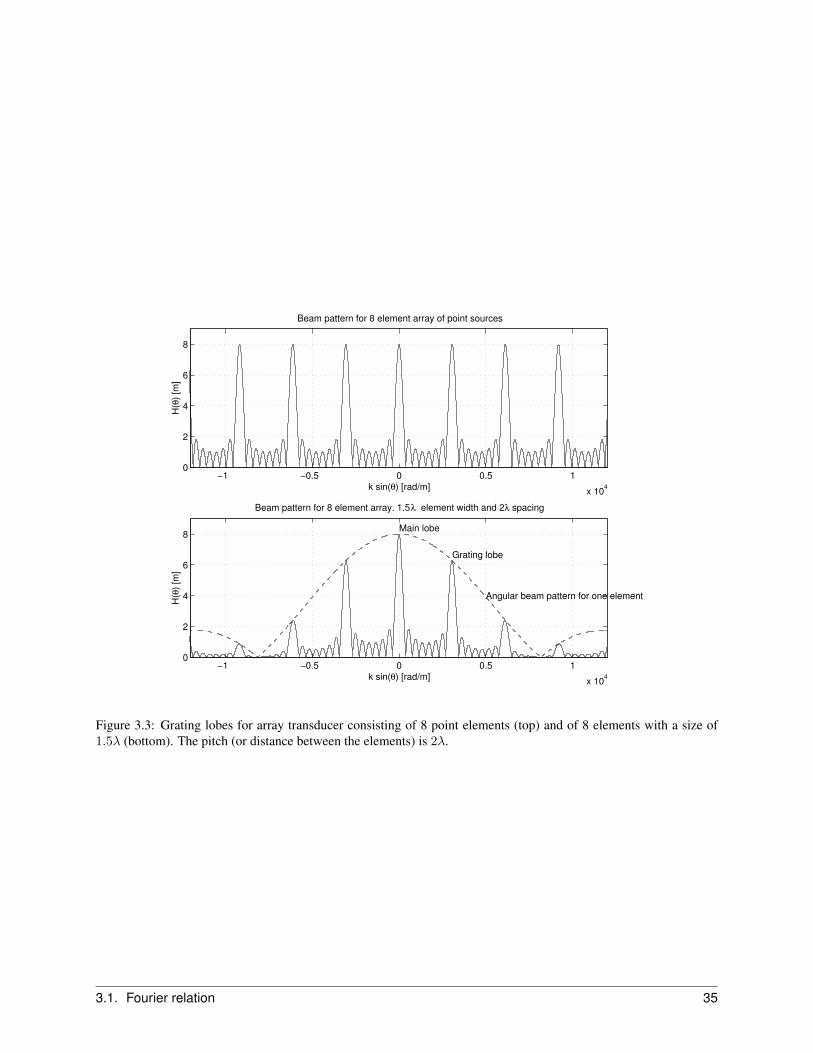
where aps(x) is the aperture function for the individual elements, dx is the spacing (pitch) between the centers of theindividual elements, and N is the number of elements in the array. Using the Fourier relationship the angular beampattern can be described by

Hp(θ) = Hps(θ)Hper(θ), (3.13)

whereN/2∑

n=−N/2

δ(x− dxn)↔ Hper(θ) =

N/2∑n=−N/2

e−jndxksinθ. =

N/2∑n=−N/2

e−j2πfsinθc ndx . (3.14)

Summing the geometric series gives

Hper(θ) =sin((N + 1)k2dx sin θ

)sin(k2dx sin θ

) (3.15)

is the Fourier transform of series of delta functions. This function repeats itself with a period that is a multiple of

π =k

2dx sin θ

sin θ =π

kdx=

λ

dx. (3.16)

This repetitive function gives rise to the grating lobes in the field. An example is shown in Fig. 3.3.

The grating lobes are due to the periodic nature of the array, and corresponds to sampling of a continuous time signal.The grating lobes will be outside a ±90 deg. imaging area if

λ

dx= 1

dx = λ (3.17)

Often the beam is steered in a direction and in order to ensure that grating lobes do not appear in the image, the spacingor pitch of the elements is selected to be dx = λ/2. This also includes ample margin for the modern transducers thatoften have a very broad bandwidth.

An array beam can be steered in a direction by applying a time delay on the individual elements. The difference inarrival time for a given direction θ0 is

τ =dx sin θ0

c(3.18)

Steering in a direction θ0 can, therefore, be accomplished by using

sin θ0 =cτ

dx(3.19)

where τ is the delay to apply to the signal on the element closest to the center of the array. A delay of 2τ is thenapplied on the second element and so forth. The beam pattern for the grating lobe is then replaced by

Hper(θ) =sin(

(N + 1)k2dx sin(θ − cτ

dx

))sin(k2dx sin

(θ − cτ

dx

)) . (3.20)

Notice that the delay is independent of frequency, since it is essentially only determined by the speed of sound.


−1 −0.5 0 0.5 1

x 104

0

2

4

6

8

k sin(θ) [rad/m]

H(θ

) [m

]

Beam pattern for 8 element array of point sources

−1 −0.5 0 0.5 1

x 104

0

2

4

6

8

k sin(θ) [rad/m]

H(θ

) [m

]

Beam pattern for 8 element array. 1.5 λ element width and 2λ spacing

Main lobe

Grating lobe

Angular beam pattern for one element

Figure 3.3: Grating lobes for array transducer consisting of 8 point elements (top) and of 8 elements with a size of1.5λ (bottom). The pitch (or distance between the elements) is 2λ.

3.1. Fourier relation 35

3.2 Focusing

The essence of focusing an ultrasound beam is to align the pressure fields from all parts of the aperture to arrive atthe field point at the same time. This can be done through a physically curved aperture, through a lens in front of theaperture, or by the use of electronic delays for multi-element arrays. All seek to align the arrival of the waves at agiven point through delaying or advancing the fields from the individual elements. The delay (positive or negative) isdetermined using ray acoustics. The path length from the aperture to the point gives the propagation time and this isadjusted relative to some reference point. The propagation from the center of the aperture element to the field point is

ti =1

c

√(xi − xf )2 + (yi − yf )2 + (zi − zf )2 (3.21)

where (xf , yf , zf ) is the position of the focal point, (xi, yi, zi) is the center for the physical element number i, c is thespeed of sound, and ti is the calculated propagation time.

A point is selected on the whole aperture as a reference for the imaging process. The propagation time for this is

tc =1

c

√(xc − xf )2 + (yc − yf )2 + (zc − zf )2 (3.22)

where (xc, yc, zc) is the reference center point on the aperture. The delay to use on each element of the array is then

∆ti =1

c

(√(xc − xf )2 + (yc − yf )2 + (zc − zf )2 −

√(xi − xf )2 + (yi − yf )2 + (zi − zf )2

)(3.23)

Notice that there is no limit on the selection of the different points, and the beam can, thus, be steered in a preferreddirection.

The arguments here have been given for emission from an array, but they are equally valid during reception of theultrasound waves due to acoustic reciprocity. At reception it is also possible to change the focus as a function of timeand thereby obtain a dynamic tracking focus. This is used by all modern ultrasound scanners, Beamformers based onanalog technology makes it possible to create several receive foci and the newer digital scanners change the focusingcontinuously for every depth in receive. A single focus is only possible in transmit and composite imaging is thereforeoften used in modern imaging. Here several pulse emissions with focusing at different depths in the same direction areused and the received signals are combined to form one image focused in both transmit and receive at different depths(composit imaging).

The focusing can, thus, be defined through time lines as:

From time Focus at0 x1, y1, z1

t1 x1, y1, z1

t2 x2, y2, z2

......

For each focal zone there is an associated focal point and the time from which this focus is used. The arrival time fromthe field point to the physical transducer element is used for deciding which focus is used. Another possibility is to setthe focusing to be dynamic, so that the focus is changed as a function of time and thereby depth. The focusing is thenset as a direction defined by two angles and a starting point on the aperture.

Section 3.1 showed that the side and grating lobes of the array can be reduced by employing apodization of theelements. Again a fixed function can be used in transmit and a dynamic function in receive defined by


From time Apodize with0 a1,1, a1,2, · · · a1,Ne

t1 a1,1, a1,2, · · · a1,Ne

t2 a2,1, a2,2, · · · a2,Ne

t3 a3,1, a3,2, · · · a3,Ne...

...

Here a1,1 is the amplitude scaling value multiplied onto element 1 after time instance t1. Typically a Hammingor Gaussian shaped function is used for the apodization. In receive the width of the function is often increased tocompensate for attenuation effects and for keeping the point spread function roughly constant. The F-number definedby

F =D

L(3.24)

where L is the total width of the active aperture and D is the distance to the focus, is often kept constant. More of theaperture is often used for larger depths and a compensation for the attenuation is thereby partly made. An example ofthe use of dynamic apodization is given in Section 3.6.

3.3 Fields from array transducers

Most modern scanners use arrays for generating and receiving the ultrasound fields. These fields are quite simple tocalculate, when the spatial impulse response for a single element is known. This is the approach used in the Field IIprogram, and this section will extend the spatial impulse response to multi element transducers and will elaborate onsome of the features derived for the fields in Section 3.1.

Since the ultrasound propagation is assumed to be linear, the individual spatial impulse responses can simply be added.If he(~rp, t) denotes the spatial impulse response for the element at position ~ri and the field point ~rp, then the spatialimpulse response for the array is

ha(~rp, t) =

N−1∑i=0

he(~ri, ~rp, t), (3.25)

assuming all N elements to be identical.

Let us assume that the elements are very small and the field point is far away from the array, so he is a Dirac function.Then

ha(~rp, t) =k

Rp

N−1∑i=0

δ(t− |~ri − ~rp|c

) (3.26)

when Rp = |~ra−~rp|, k is a constant of proportionality, and ~ra is the position of the array. Thus, ha is a train of Diracpulses. If the spacing between the elements is D, then

ha(~rp, t) =k

Rp

N−1∑i=0

δ

(t− |~ra + iD~re − ~rp|

c

), (3.27)

where ~re is a unit vector pointing in the direction along the elements. The geometry is shown in Fig. 3.4.

The difference in arrival time between elements far from the transducer is

∆t =D sin Θ

c. (3.28)

The spatial impulse response is, thus, a series of Dirac pulses separated by ∆t.

ha(~rp, t) ≈k

Rp

N−1∑i=0

δ

(t− Rp

c− i∆t

). (3.29)

3.3. Fields from array transducers 37

θ

Array elements

D

re

ra

Figure 3.4: Geometry of linear array (from [9], Copyright Cambridge University Press).

The time between the Dirac pulses and the shape of the excitation determines whether signals from individual elementsadd or cancel out. If the separation in arrival times corresponds to exactly one or more periods of a sine wave, thenthey are in phase and add constructively. Thus, peaks in the response are found for

n1

f=D sin Θ

c. (3.30)

The main lobe is found for Θ = 0 and the next maximum in the response is found for

Θ = arcsin

(c

fD

)= arcsin

(λ

D

). (3.31)

For a 3 MHz array with an element spacing of 1 mm, this amounts to Θ = 31◦, which will be within the imageplane. The received response is, thus, affected by scatterers positioned 31◦ off the image axis, and they will appear inthe lines acquired as grating lobes. The first grating lobe can be moved outside the image plane, if the elements areseparated by less than a wavelength. Usually, half a wavelength separation is desirable, as this gives some margin fora broad-band pulse and beam steering.

The beam pattern as a function of angle for a particular frequency can be found by Fourier transforming ha

Ha(f) =k

Rp

N−1∑i=0

exp

(−j2πf

(Rpc

+ iD sin Θ

c

))

= exp(−j2πRpc

)k

Rp

N−1∑i=0

exp

(−j2πf D sin Θ

c

)i(3.32)

=sin(πf D sin Θ

c N)

sin(πf D sin Θc )

exp(−jπf(N − 1)D sin Θ

c)k

Rpexp(−j2πRp

c).

The terms exp(−j2πRpc ) and exp(−jπf(N − 1)D sin Θc ) are constant phase shifts and play no role for the amplitude

of the beam profile. Thus, the amplitude of the beam profile is

|Ha(f)| =

∣∣∣∣∣ kRp sin(NπDλ sin Θ)

sin(πDλ sin Θ)

∣∣∣∣∣ . (3.33)

The beam profile at 3 MHz is shown in Fig. 3.5 for a 64-element array with D = 1 mm.


-80 -60 -40 -20 0 20 40 60 80-40

-35

-30

-25

-20

-15

-10

-5

0

Angle [deg]

Norm

aliz

ed a

mplit

ude [dB

]

Figure 3.5: Far-field continuous wave beam profile at 3 MHz for linear array consisting of 64 point sources with aninter-element spacing of 1 mm (from [9], Copyright Cambridge University Press).

3.3. Fields from array transducers 39

-80 -60 -40 -20 0 20 40 60 80-40

-30

-20

-10

0

Angle [deg]

Norm

. m

ax. am

p. [d

B]

Array of point sources

-80 -60 -40 -20 0 20 40 60 80-40

-30

-20

-10

0

Angle [deg]

Norm

. m

ax. am

p. [d

B]

Array of rectangular sources

Figure 3.6: Beam profiles for an array consisting of point sources (top) or rectangular elements (bottom). The excita-tion pulse has a frequency of 3 MHz and the element spacing is 1 mm. The distance to the field point is 100 mm (from[9], Copyright Cambridge University Press).

Several factors change the beam profile for real, pulsed arrays compared with the analysis given here. First, the ele-ments are not points, but rather are rectangular elements with an off-axis spatial impulse response markedly differentfrom a Dirac pulse. Therefore, the spatial impulse responses of the individual elements will overlap and exact cancel-lation or addition will not take place. Second, the excitation pulse is broad band, which again influences the sidelobes.Examples of simulated responses are shown in Fig. 3.6.

The top graph shows an array of 64 point sources excited with a Gaussian 3 MHz pulse with Br = 0.2. The spacebetween the elements is 1 mm. The maximum of the response at a radial position of 100 mm from the transducer istaken. The bottom graph shows the response when rectangular elements of 1 × 6 mm are used. This demonstrates thesomewhat crude approximation of using the far-field point source CW response to characterize arrays.

Fig. 3.7 shows the different point spread functions encountered when a phased array is used to scan over a 15 cmdepth. The array consists of 128 elements each 0.2 × 5 mm in size, and the kerf between the elements is 0.05 mm.The transmit focus is at 70 mm, and the foci are at 30, 70, and 110 mm during reception. Quite complicated pointspread functions are encountered, and they vary substantially with depth in tissue. Notice especially the edge waves,which dominate the response close to the transducer. The edge effect can be reduced by weighting responses fromdifferent elements. This is also called apodization. The excitation pulses to elements at the transducer edge arereduced, and this diminishes the edge waves. More examples are shown below in Section 3.6.

3.4 Imaging with arrays

Basically there are three different kinds of images acquired by multi-element array transducers, i.e. linear, convex, andphased as shown in Figures 3.8, 3.10, and 3.11. The linear array transducer is shown in Fig. 3.8. It selects the region of


−40 −30 −20 −10 0 10 20 30 40

0

2

4

6

8

10

12

14

16

18

20x 10

−5

Lateral displacement [mm]

Tim

e [

s]

Transmit focus (70 mm)

30 mm receive focus

70 mm receive focus

110 mm receive focus

Figure 3.7: Point spread functions for different positions in a B-mode image. Onehundredtwentyeight 0.2 × 5 mmelements are used for generating and receiving the pulsed field. Three different receive foci are used. The contoursshown are from 0 to -24 dB in steps of 6 dB relative to the maximum at the particular field point (from [9], CopyrightCambridge University Press).

Figure 3.8: Linear array transducer for obtaining a rectangular cross-sectional image.

3.4. Imaging with arrays 41

Electronic focusing

t

0

Excitation pulses

Transducerelements

Beam shape

(a)

t

0

Excitation pulses

Transducerelements

Beam shape

Beam steering and focusing

(b)

Figure 3.9: Electronic focusing and steering of an ultrasound beam.

investigation by firing a set of elements situated over the region. The beam is moved over the imaging region by firingsets of contiguous elements. Focusing in transmit is achieved by delaying the excitation of the individual elements, soan initially concave beam shape is emitted, as shown in Fig. 3.9.

The beam can also be focused during reception by delaying and adding responses from the different elements. Acontinuous focus or several focal zones can be maintained as explained in Section 3.2. Only one focal zone is possiblein transmit, but a composite image using a set of foci from several transmissions can be made. Often 4 to 8 zonescan be individually placed at selected depths in modern scanners. The frame rate is then lowered by the number oftransmit foci.

The linear arrays acquire a rectangular image, and the arrays can be quite large to cover a sufficient region of interest(ROI). A larger area can be scanned with a smaller array, if the elements are placed on a convex surface as shown inFig. 3.10. A sector scan is then obtained. The method of focusing and beam sweeping during transmit and receive isthe same as for the linear array, and a substantial number of elements (often 128 or 256) is employed.

The convex and linear arrays are often too large to image the heart when probing between the ribs. A small array sizecan be used and a large field of view attained by using a phased array as shown in Fig. 3.11. All array elements areused here both during transmit and receive. The direction of the beam is steered by electrically delaying the signals toor from the elements, as shown in Fig. 3.9b. Images can be acquired through a small window and the beam rapidlysweeped over the ROI. The rapid steering of the beam compared to mechanical transducers is of especial importancein flow imaging. This has made the phased array the choice for cardiological investigations through the ribs.

More advanced arrays are even being introduced these years with the increase in number of elements and digitalbeamforming. Especially elevation focusing (out of the imaging plane) is important. A curved surface as shown inFig. 3.12 is used for obtaining the elevation focusing essential for an improved image quality. Electronic beamformingcan also be used in the elevation direction by dividing the elements in the elevation direction. The elevation focusingin receive can then be dynamically controlled for e.g. the array shown in Fig. 3.13.


Figure 3.10: Convex array transducer for obtaining a polar cross-sectional image.

Figure 3.11: Phased array transducer for obtaining a polar cross-sectional image using a transducer with a smallfoot-print.


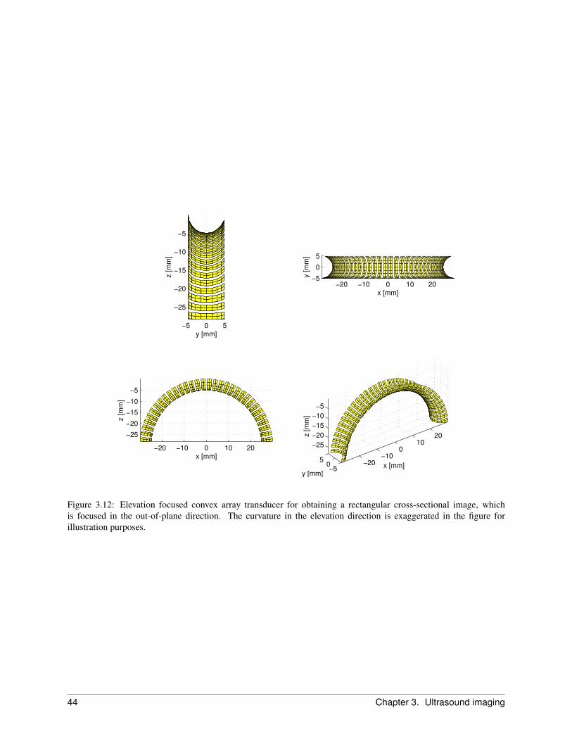
−5 0 5

−25

−20

−15

−10

−5

y [mm]

z [m

m]

−20 −10 0 10 20−5

0

5

x [mm]

y [m

m]

−20 −10 0 10 20

−25

−20

−15

−10

−5

x [mm]

z [m

m]

−20−10

010

20

−50

5

−25

−20

−15

−10

−5

x [mm]y [mm]

z [m

m]

Figure 3.12: Elevation focused convex array transducer for obtaining a rectangular cross-sectional image, whichis focused in the out-of-plane direction. The curvature in the elevation direction is exaggerated in the figure forillustration purposes.


−5 0 5

−20

−15

−10

−5

y [mm]

z [m

m]

−20 −10 0 10 20

−5

0

5

x [mm]y [m

m]

−20 −10 0 10 20

−20

−15

−10

−5

x [mm]

z [m

m]

−20−10

010

20

−50

5

−20

−15

−10

−5

x [mm]y [mm]

z [m

m]

Figure 3.13: Elevation focused convex array transducer with element division in the elevation direction. The curvaturein the elevation direction is exaggerated in the figure for illustration purposes


3.5 Simulation of ultrasound imaging

One of the first steps in designing an ultrasound system is the selection of the appropriate number of elements for thearray transducers and the number of channels for the beamformer. The focusing strategy in terms of number of focalzones and apodization must also be determined. These choices are often not easy, since it is difficult to determinethe effect in the resulting images of increasing the number of channels and selecting more or less advanced focusingschemes. It is therefore beneficial to simulate the whole imaging system in order to quantify the image quality.

The program Field II was rewritten to make it possible to simulate the whole imaging process with time varyingfocusing and apodization as described in [38] and [21]. This has paved the way for doing realistic simulated imagingwith multiple focal zones for transmission and reception and for using dynamic apodization. It is hereby possible tosimulate ultrasound imaging for all image types including flow images, and the purpose of this section is to presentsome standard simulation phantoms that can be used in designing and evaluating ultrasound transducers, beamformersand systems. The phantoms described can be divided into ordinary string/cyst phantoms, artificial human phantomsand flow imaging phantoms. The ordinary computer phantoms include both a string phantoms for evaluating the pointspread function as a function of spatial positions as well as a cyst/string phantom. Artificial human phantoms of a fetusin the third month of development and an articial kedney are also shown. The simulation of flow and the associatedphantoms will be described in Section 4.5. All the phantoms can be used with any arbitrary transducer configurationlike single element, linear, convex, or phased array transducers, with any apodization and focusing scheme.

3.5.1 Simulation model

The first simple treatment of ultrasound is often based on the reflection and transmission of plane waves. It is assumedthat the propagating wave impinges on plane boundaries between tissues with different mean acoustic properties. Suchboundaries are rarely found in the human body, and seldom show on ultrasound images. This is demonstrated by theimage shown in Fig. 3.14. Here the skull of the fetus is not clearly marked. It is quite obvious that there is a clearboundary between the fetus and the surrounding amniotic fluid. The skull boundary is not visible in the image, becausethe angle between the beam and the boundary has a value such that the sound bounces off in another direction, and,therefore, does not reach the transducer. Despite this, the extent of the head can still be seen. This is due to thescattering of the ultrasound wave. Small changes in density, compressibility, and absorption give rise to a scatteredwave radiating in all directions. The backscattered field is received by the transducer and displayed on the screen. Onemight well argue that scattering is what makes ultrasound images useful for diagnostic purposes, and it is, as will beseen later, the physical phenomena that makes detection of blood velocities possible. Ultrasound scanners are, in fact,optimized to show the backscattered signal, which is considerably weaker than that found from reflecting boundaries.Such reflections will usually be displayed as bright white on the screen, and can potentially saturate the receivingcircuits in the scanner. An example can be seen at the neck of the fetus, where a structure is perpendicular to the beam.This strong reflection saturates the input amplifier of this scanner. Typical boundary reflections are encountered fromthe diaphragm, blood vessel walls, and organ boundaries.

An enlarged view of an image of a liver is seen in Fig. 3.15. The image has a grainy appearance, and not a homogeneousgray or black level as might be expected from homogeneous liver tissue. This type of pattern is called speckle. Thedisplayed signals are the backscatter from the liver tissue, and are due to connective tissue, cells, and fibrious tissue inthe liver. These structures are much smaller than one wavelength of the ultrasound, and the speckle pattern displayeddoes not directly reveal physical structure. It is rather the constructive and destructive interference of scattered signalsfrom all the small structures. So it is not possible to visualize and diagnose microstructure, but the strength of thesignal is an indication of pathology. A strong signal from liver tissue, making a bright image, is, e.g., an indication ofa fatty or cirrhotic liver.

As the scattered wave emanates from numerous contributors, it is appropriate to characterize it in statistical terms. Theamplitude distribution follows a Gaussian distribution [39], and is, thus, fully characterized by its mean and variance.The mean value is zero since the scattered signal is generated by differences in the tissue from the mean acousticproperties.


Amniotic fluid

Head

Mouth

Spine

Boundary of placenta

Amniotic fluid

Foot

Figure 3.14: Ultrasound image of a 13th week fetus. The markers at the border of the image indicate one centimeter(from [9], Copyright Cambridge University Press).

3.5. Simulation of ultrasound imaging 47

Figure 3.15: 4 × 4 cm image of a human liver from a healthy 28-year-old man. The completely dark areas are bloodvessels (from [9], Copyright Cambridge University Press).

Although the backscattered signal is characterized in statistical terms, one should be careful not to interpret the signalas random in the sense that a new set of values is generated for each measurement. The same signal will result, whena transducer is probing the same structure, if the structure is stationary. Even a slight shift in position will yield abackscattered signal correlated with that from the adjacent position. The shift over which the signals are correlated isessentially dependent on the extent of the ultrasound field. This can also be seen from the image in Fig. 3.15, as thelaterally elongated white speckles in the image indicate transverse correlation. The extent of these speckle spots is arough indication of the point spread function of the system.

The correlation between different measurements is what makes it possible to estimate blood velocities with ultrasound.As there is a strong correlation for small movements, it is possible to detect shifts in position by comparing or, morestrictly, correlating successive measurements of moving structure, e.g., blood cells.

Since the backscattered signal depends on the constructive and destructive interference of waves from numerous smalltissue structures, it is not meaningful to talk about the reflection strength of the individual structures. Rather, it isthe deviations within the tissue and the composition of the tissue that determine the strength of the returned signal.The magnitude of the returned signal is, therefore, described in terms of the power of the scattered signal. Since thesmall structures reradiate waves in all directions and the scattering structures might be ordered in some direction, thereturned power will, in general, be dependent on the relative position between the ultrasound emitter and receiver.Such a medium is called anisotropic, examples of which are muscle and kidney tissue. By comparison, liver tissue isa fairly isotropic scattering medium, when its major vessels are excluded, and so is blood.

It is, thus, important that the simulation approach models the scattering mechanisms in the tissue. This is essentiallywhat the model derived in Chapter 2 does. Here the received signal from the transducer is:

pr(~r, t) = vpe(t) ?tfm(~r) ?

rhpe(~r, t) (3.34)

where ?r denotes spatial convolution. vpe is the pulse-echo impulse, which includes the transducer excitation and the

electro-mechanical impulse response during emission and reception of the pulse. fm accounts for the inhomogeneities


in the tissue due to density and propagation velocity perturbations which give rise to the scattered signal. hpe is thepulse-echo spatial impulse response that relates the transducer geometry to the spatial extent of the scattered field.Explicitly written out these terms are:

vpe(t) =ρ

2c2Em(t) ?

t

∂3v(t)

∂t3, fm(~r1) =

∆ρ(~r)

ρ− 2∆c(~r)

c, hpe(~r, t) = ht(~r, t) ∗ hr(~r, t) (3.35)

So the received response can be calculated by finding the spatial impulse response for the transmitting and receivingtransducer and then convolving with the impulse response of the transducer. A single RF line in an image can becalculated by summing the response from a collection of scatterers in which the scattering strength is determined bythe density and speed of sound perturbations in the tissue. Homogeneous tissue can thus be made from a collectionof randomly placed scatterers with a scattering strength with a Gaussian distribution, where the variance of the distri-bution is determined by the backscattering cross-section of the particular tissue. This is the approach taken in thesenotes.

The computer phantoms typically consist of 100,000 or more discrete scatterers, and simulating 50 to 128 RF lines cantake several days depending on the computer used. It is therefore beneficial to split the simulation into concurrentlyrun sessions. This can easily be done by first generating the scatterer’s position and amplitude and then storing them ina file. This file can then the be used by a number of workstations to find the RF signal for different imaging directions,which are then stored in separate files; one for each RF line. These files are then used to assemble an image. This isthe approach used for the simulations shown here in which 3 Pentium Pro 200 MHz PCs can generate one phantomimage over night using Matlab 5 and the Field II program.

3.6 Synthetic phantoms

The first synthetic phantom consists of a number of point targets placed with a distance of 5 mm starting at 15 mmfrom the transducer surface. A linear sweep image of the points is then made and the resulting image is compressedto show a 40 dB dynamic range. This phantom is suited for showing the spatial variation of the point spread functionfor a particular transducer, focusing, and apodization scheme.

Twelve examples using this phantom are shown in Fig. 3.16. The top graphs show imaging without apodization andthe bottom graphs show images when a Hanning window is used for apodization in both transmit and receive. A 128elements transducer with a nominal frequency of 3 MHz was used. The element height was 5 mm, the width was awavelength and the kerf 0.1 mm. The excitation of the transducer consisted of 2 periods of a 3 MHz sinusoid witha Hanning weighting, and the impulse response of both the emit and receive aperture also was a two cycle, Hanningweighted pulse. In the graphs A – C, 64 of the transducer elements were used for imaging, and the scanning wasdone by translating the 64 active elements over the aperture and focusing in the proper points. In graph D and E 128elements were used and the imaging was done solely by moving the focal points.

Graph A uses only a single focal point at 60 mm for both emission and reception. B also uses reception focusing atevery 20 mm starting from 30 mm. Graph C further adds emission focusing at 10, 20, 40, and 80 mm. D applies thesame focal zones as C, but uses 128 elements in the active aperture.

The focusing scheme used for E and F applies a new receive profile for each 2 mm. For analog beamformers this isa small zone size. For digital beamformers it is a large zone size. Digital beamformer can be programmed for eachsample and thus a ”continuous” beamtracking can be obtained. In imaging systems focusing is used to obtain highdetail resolution and high contrast resolution preferably constant for all depths. This is not possible, so compromisesmust be made. As an example figure F shows the result for multiple transmit zones and receive zones, like E, but nowa restriction is put on the active aperture. The size of the aperture is controlled to have a constant F-number (depth offocus in tissue divided by width of aperture), 4 for transmit and 2 for receive, by dynamic apodization. This gives amore homogeneous point spread function throughout the full depth. Especially for the apodized version. Still it canbe seen that the composite transmit can be improved in order to avoid the increased width of the point spread functionat e.g. 40 and 60 mm.

3.6. Synthetic phantoms 49

Axia

l d

ista

nce

[m

m]

A


−10 0 10

20

40

60

80

100

120

B C D E F

Axia

l d

ista

nce

[m

m]

A


−10 0 10

20

40

60

80

100

120

B C D E F

Figure 3.16: Point target phantom imaged for different set-up of transmit and receive focusing and apodization. Seetext for an explanation of the set-up.



Axia

l d

ista

nce

[m

m]

−20 −10 0 10 20

35

40

45

50

55

60

65

70

75

80

85

Figure 3.17: Computer phantom with point targets, cyst regions, and strongly reflecting regions.

The next phantom consists of a collection of point targets, five cyst regions, and five highly scattering regions. Thiscan be used for characterizing the contrast-lesion detection capabilities of an imaging system. The scatterers in thephantom are generated by finding their random position within a 60 × 40 × 15 mm cube, and then ascribe a Gaussiandistributed amplitude to the scatterers. If the scatterer resides within a cyst region, the amplitude is set to zero.Within the highly scattering region the amplitude is multiplied by 10. The point targets has a fixed amplitude of 100,compared to the standard deviation of the Gaussian distributions of 1. A linear scan of the phantom was done witha 192 element transducer, using 64 active elements with a Hanning apodization in transmit and receive. The elementheight was 5 mm, the width was a wavelength and the kerf 0.05 mm. The pulses where the same as used for the pointphantom mentioned above. A single transmit focus was placed at 60 mm, and receive focusing was done at 20 mmintervals from 30 mm from the transducer surface. The resulting image for 100,000 scatterers is shown in Fig. 3.17.A homogeneous speckle pattern is seen along with all the features of the phantom.

3.7 Anatomic phantoms

The anatomic phantoms are attempts to generate images as they will be seen from real human subjects. This is done bydrawing a bitmap image of scattering strength of the region of interest. This map then determines the factor multipliedonto the scattering amplitude generated from the Gaussian distribution, and models the difference in the density andspeed of sound perturbations in the tissue. Simulated boundaries were introduced by making lines in the scatterer mapalong which the strong scatterers were placed. This is marked by completely white lines shown in the scatterer maps.The model is currently two-dimensional, but can readily be expanded to three dimensions. Currently, the elevationdirection is merely made by making a 15 mm thickness for the scatterer positions, which are randomly distributed inthe interval.

Two different phantoms have been made; a fetus in the third month of development and a left kidney in a longitudinal

3.7. Anatomic phantoms 51


Axia

l d

ista

nce

[m

m]

Fetus scatter map

−40 −20 0 20 40

20

40

60

80

Simulated fetus image

Figure 3.18: Simulation of artificial fetus.

scan. For both was used 200,000 scatterers randomly distributed within the phantom, and with a Gaussian distributedscatterer amplitude with a standard deviation determined by the scatterer map. The phantoms were scanned with a 5MHz 64 element phased array transducer with λ/2 spacing and Hanning apodization. A single transmit focus 70 mmfrom the transducer was used, and focusing during reception is at 40 to 140 mm in 10 mm increments. The imagesconsists of 128 lines with 0.7 degrees between lines.

Fig. 3.19 shows the artificial kidney scatterer map on the left and the resulting image on the right. Note especially thebright regions where the boundary of the kidney is orthogonal to the ultrasound, and thus a large signal is received.Note also the fuzziness of the boundary, where they are parallel with the ultrasound beam, which is also seen on actualultrasound scans. Fig. 3.18 shows the fetus. Note how the anatomy can be clearly seen at the level of detail of thescatterer map. The same boundary features as for the kidney image is also seen.

The images have many of the features from real scan images, but still lack details. This can be ascribed to the lowlevel of details in the bitmap images, and that only a 2D model is used. But the images do show great potential formaking powerful fully synthetic phantoms, that can be used for image quality evaluation.



Axia

l dis

tance [m

m]

Kidney scatter map

−50 0 50

20

40

60

80

100

Simulated kidney image

Figure 3.19: Simulation of artificial kidney.

3.7. Anatomic phantoms 53

54

CHAPTER

FOUR

Ultrasound Velocity Imaging

This chapter is taken from the book chapter:

Jørgen Arendt Jensen :

Ultrasound Velocity Imaging

Ultrasound Imaging and Therapy. ed. / Aaron Fenster; James C. Lacefield. CRCTaylor and Francis Group, 2015. p. 65-99 (Imaging in medical diagnosis andtherapy)

55

4.1 Introduction: Blood Velocity Estimation Systems

This Chapter gives an introduction to velocity estimation in medical ultrasound, which is primarily used in cardio-vascular imaging, but it can also be applied in e.g. strain imaging and tissue motion estimation. The Chapter givesa brief introduction to the human circulation to establish the requirements on blood velocity estimation systems.A simple model for the interaction between ultrasound and point scatterers is derived in Section 4.4 based on theinformation about scattering from blood in Section 4.3. The model is used in the derivation of velocity estimators basedon the signal’s frequency content (Section 4.6), phase shift (Section 4.7), and time shift (Section 4.8). These Sectionsshould give a brief introduction to the function of the most prominent methods used in current commercial ultrasoundscanners. Newer and more experimental techniques are described in the Sections on vector velocity imaging, syntheticaperture imaging and other applications in Sections 4.9 to 4.12.

The Chapter is necessarily brief in covering the many topics of this field, and the reader is referred to the more in-depthtreatment of the topics in [9, 40, 41, 42, 43] along with the references given in the text.

4.2 The human circulation

The major arteries and veins in the human circulation are shown in Fig. 4.1, and the dimensions are indicated inTable 4.1. Their diameters span from cm to microns and the velocities from m/s to less than mm/s in the capillaries.As illustrated, the vessel constantly curves and branches and repeatedly changes dimensions [44]. The blood flowis pulsatile, and the velocity rapidly changes both magnitude and direction as can be seen from the large differencebetween peak and mean velocities. In addition the peak Reynolds number is often above 2000, which indicatesdisturbed or turbulent flow in parts of the cardiac cycle.

All of these factors should be considered when devising a system for measuring blood the velocity in the humancirculation. Foremost it must be a fast measurement system with 1 – 20 ms temporal resolution to follow the changesin velocity due to the acceleration from the pulsation. It should also have sub-millimeter spatial resolution in orderto see changes in flow over space and visualize small vessels. A real-time system is also beneficial, since the flowpatterns change rapidly, and it must be possible to quickly find the sites of flow. The system should ideally also becapable of finding and visualizing flow in all directions, since turbulent flow and vortices exists throughout the humancirculation. Modern medical ultrasound systems can fulfill many of these demands, and the remaining part of thisChapter describes the physics and signal processing needed to perform velocity estimation along the ultrasound beamand in other directions.

4.3 Ultrasound scattering from blood

The constituents of blood are shown in Table 4.2. The most prominent part is the erythrocytes (red blood cells), wherea mm3 of blood contains roughly 5 million cells. The resolution of ultrasound systems is at best on the order of thecube of the wavelength λ3, which is given by λ = c/f0, where c is the speed of sound and f0 the center frequency.For a 6 MHz system λ = 0.26 mm, which is much larger than a single cell. An ultrasound system, thus, only observesa large, random collection of cells.

The scattering from a single point scatterer or small cell can be described by the differential scattering cross section,σd. It is defined as the power scattered per unit solid angle at some angle Θs divided by the incident intensity [11, 51]:

σd(Θs) =V 2e π

2

λ4

[κe − κ0

κ0+ρe − ρ0

ρecos Θs

]2

, (4.1)

where Ve is the volume of the scatterer, ρe is a small perturbation in density and κe in compressibility from their meanvalues ρ0, κ0. This results in a scattered field as shown in Fig. 4.2, where the scattering is dependent on the angle. Itcan, however, be seen that a signal is received in all directions.

56 Chapter 4. Ultrasound Velocity Imaging

Venous circulation

Arterial circulation

External jugular

Internal jugular

Subclavian

Axillary

Superior vena cava

Cephalic

Brachial

BasilicMedian cubital

Inferior mesenteric

Superior mesentric

UlnarRadial

Inferior vena cava

IliacDeep palmar venous arch

Deep femoral

Femoral

Great saphenous

Popliteal

Anterior tibial

Posterior tibial

Peroneal

Cerebrals

Internal carotid

External carotidCommon carotid

InnominateSubclavian

Axillary

Deep brachialBrachialRenal

Superior mesentricInferior mesentric

Abdominal aortaInterosseousUlnarRadial

Common iliacInternal iliacDeep palmer archSuperficial palmer archCommon femoralDeep femoralSuperficial femoral

Popliteal

Anterior tibialPosterior tibialPeroneal

Dorsalis pedis

Figure 4.1: Major arteries and veins in the body (reprinted with permission from Abbott Laboratories, Illinois, USA).

θs

Monopole scattering

Dipole scattering

Combinedscattering

Direction ofincident field

Backscattering

Forw

ard

scattering

Figure 4.2: Monopole and dipole scattering from a perturbation in either compressibility or density (from [9]).

4.3. Ultrasound scattering from blood 57

Table 4.1: Typical dimensions and flows of vessels in the human vascular system (data taken from [45, 46] and Tableadapted from [9]).

Internal Wall Young’sdiameter thickness Length modulus

Vessel cm cm cm N/m2 · 105

Ascending aorta 1.0 – 2.4 0.05 – 0.08 5 3 – 6Descending aorta 0.8 – 1.8 0.05 – 0.08 20 3 – 6Abdominal aorta 0.5 – 1.2 0.04 – 0.06 15 9 – 11Femoral artery 0.2 – 0.8 0.02 – 0.06 10 9 – 12Carotid artery 0.2 – 0.8 0.02 – 0.04 10 – 20 7 – 11Arteriole 0.001 – 0.008 0.002 0.1 – 0.2Capillary 0.0004 – 0.0008 0.0001 0.02 – 0.1Inferior vena cava 0.6 – 1.5 0.01 – 0.02 20 – 40 0.4 – 1.0

Peak Mean Reynolds Pulse propaga-velocity velocity number tion velocity

Vessel cm/s cm/s (peak) cm/sAscending aorta 20 – 290 10 – 40 4500 400 – 600Descending aorta 25 – 250 10 – 40 3400 400 – 600Abdominal aorta 50 – 60 8 – 20 1250 700 – 600Femoral artery 100 – 120 10 – 15 1000 800 – 1030Common Carotid artery (range) 68 – 171 19-59 600 – 1100Common Carotid artery (mean) 108 39 600 – 1100Arteriole 0.5 – 1.0 0.09Capillary 0.02 – 0.17 0.001Inferior vena cava 15 – 40 700 100 – 700

Mass Adiabaticdensity compressibility Size Particlesg/cm3 10−12 cm/dyne µm per mm3

Erythrocytes 1.092 34.1 2× 7 5 · 106

Leukocytes - - 9 – 25 8 · 103

Platelets - - 2 – 4 250− 500 · 103

Plasma 1.021 40.9 - -0.9% saline 1.005 44.3 - -

Table 4.2: Properties of the main components of blood. Data from [47, 48, 49, 50] and Table adapted from [9].


The signal received by the ultrasound transducer is therefore independent of the orientation of the vessel and it canbe modeled as a random, Gaussian signal, as it emanates from a large collection of independent random scatterers.This give rise to the speckle pattern seen in ultrasound images. The scattering is very weak, as the density andcompressibility perturbations are small compared to the surrounding tissue, and often the signal from blood is 20-40dB lower than from the surrounding tissue. Vessels in an ultrasound image therefore appear black.

It should be noted that the signal received is random, but the same signal is received, if the experiment is repeated forthe exact same collection of scatterers. This is a very important feature of ultrasound blood velocity signals and isheavily used in these systems, as will be clear in the following Sections. A small motion of the scatterers will thereforeyield a second signal highly correlated with the first signal, when the motion |v|Tprf is small compared to the beamwidth, and the velocity gradient is small across the scatterer collection observed. Here |v| is velocity magnitude andTprf is the time between the measurements.

4.4 Ultrasound signals from flowing blood

The derivation of velocity estimation methods is based on a model of ultrasound interaction between the moving bloodand the ultrasound pulse. The model has to capture all the main features of the real received signal without unnecessaryfeatures and complications. This section will present a simple model for this interaction, which can readily be usedfor deriving new estimators and also give basic explanations for how to optimize the techniques. It can also be furtherexpanded to the two- and three-dimensional velocity estimation methods presented in Sections 4.9 and 4.10.

The scattering from blood emanates from a large collection of independent, small point scatterers as described inSection 4.3. The one-dimensional received signal y(t) can therefore be modeled as:

y(t) = p(t) ∗ s(t), (4.2)

which is the convolution of the basic ultrasound pulse p(t) with the Gaussian, random scattering signal s(t). Theultrasound pulse for flow estimation consists of a number of sinusoidal oscillations (Mp = 4− 8) at the transducer’scenter frequency, f0, convolved with the electro-mechanical impulse response of the transducer (from excitation volt-age to pressure and from pressure to received voltage) [52]. Modern transducers are so broad band that a simpleapproximation is given by

p(t) = g(t) sin(2πf0t), (4.3)

where the envelope g(t) is one from t = 0 to Mp/f0 and zero elsewhere.

For a single point scatterer, the scattering can be modeled as a δ-function and the received signal is

y1(t) = p(t) ∗ aδ(t− 2d

c

)= ap

(t− 2d

c

), (4.4)

where d is the distance to the point, c is the speed of sound (1540 m/s in tissue), and a is the scattering amplitude.There is, thus, a propagation delay 2d/c between transmitting the signal and receiving the response. For a movingscatterer this response will change as the scatterer moves farther away from the transducer. For a scatterer velocity ofvz = |v| cos θ in the axial direction, and a time between measurements of Tprf , the second received signal is

y2(t) = p(t) ∗ aδ(t− 2d

c− 2vzTprf

c

)= ap

(t− 2d

c− 2vzTprf

c

). (4.5)

Note that vzTprf = Tprf |v| cos θ is the distance the scatterer moved along the ultrasound beam direction, where θ isthe beam-to-flow angle. There is therefore an added delay of

ts =2vzcTprf (4.6)

before the second signal is received. This is directly proportional to the velocity of the moving scatterer, and bydetermining this delay the axial velocity can directly be calculated. This can be achieved either through the phase shift

4.4. Ultrasound signals from flowing blood 59

estimator described in Section 4.7 or the time shift estimator in Section 4.8. Both estimators essentially just compareor correlate two received signals and find the shift in position between the received responses.

Combining (4.3) and (4.5) gives a model for the received signal for a number of pulse emissions [53, 54]:

y(t, i) = ap(t− 2d

c− i2vz

cTprf ) = ag(t− 2d

c− its) sin(2πf0(t− 2d

c− its)). (4.7)

Here i is the pulse emission number. For pulsed systems the received signal is measured at a single depth correspondingto a fixed time tx relative to the pulse emission. This is performed by taking out one sample from each pulse emissionto create the sampled signal. To simplify things it can assumed that the pulse is long enough and the motion slowenough, so that the pulse amplitude stays roughly constant during the observation time. The sampled signal can thensimply be written as

y(tx, i) = a sin(2πf0(tx −2d

c− its))

= −a sin(2π2vzcf0iTprf − φx). (4.8)

Here φx = 2πf0( 2dc − tx) is a fixed phase shift depending on the measurement depth. The sampling interval is Tprf

and the frequency of the sampled signal is

fp =2vzcf0, (4.9)

which is directly proportional to the velocity. Thus, estimating the frequency of this sampled signal y(tx, i) can directlyreveal the axial velocity as described in the Section 4.6 on spectral velocity estimation. Often it is advantageous toalso sample the signal in the depth direction, and this gives

ys(n, i) = ag(n∆T − 2d

c− its) sin(2πf0(n∆T − 2d

c− its)), (4.10)

which is often employed for averaging along the depth direction. Here ∆T = 1/fs is the sampling interval and fs thesampling frequency.

An illustration of the sampling process for a single moving scatterer is shown in Fig. 4.3, where the individual receivedsignals are shown on the left graph. The scatterer is moving away from the transducer, and the time between emissionand reception of the signal increases. A single sample is taken out for each received signal at the position of the redline. The resulting sampled signal is shown on the right graph, where the basic emitted pulse can be recognized. A lowvelocity will yield a long pulse and hence a low frequency of the received signal as indicated by (4.9). A high velocitywill compress the signal and thereby give a high frequency. The velocity can be found by three different methods. AFourier transform can be applied on the signal in the right graph to find the frequency as described in Section 4.6. Thephase shift can be determined between the received signals. This is described in Section 4.7. The time shift can befound by correlating consecutive received signals, i.e. cross-correlating received signals in the left graph as describedin Section 4.8.

The signal model can also be expanded to include a collection of scatterers moving at the same velocity

y(t, i) = p(t) ∗ s(t− its − iTprf ) = p(t− its − iTprf ) ∗ s(t) = p(t− its) ∗ s(t). (4.11)

as the same pulse is emitted every time. Using superposition this can just be seen as a summation of individualscatterers moving at their velocity and the model and observations made above can readily be applied.

4.4.1 Is it the Doppler effect?

The ultrasound systems for measuring velocity are often called Doppler systems implying that they rely on the Dopplershift to find the velocity. It is debatable whether this is really true. The Doppler effect can be described as a frequencyshift on the received signal. The received signal can be written as:

yD(t) = a sin(2π(1 +2vzc

)f0t) (4.12)


0 1 2 3 4 5 6 7

x 10−6

5

10

15

20

25

30

35

40

Em

issio

n n

um

be

r a

nd

sig

na

l a

mp

litu

de

[v]

Time from pulse emission [s]−0.5 0 0.5

0

1

2

3

4

5

6

7

x 10−3

Sa

mp

le t

ime

[s]

Amplitude [v]

Figure 4.3: Received signals from a single scatterer moving away from the transducer. The solid red line in the leftgraph indicates the sampling instance for the samples show on the right graph.

for a simple continuous wave source. Here the received frequency is scaled by (1+2vz/c). There is, thus, a frequencydifference of fD = 2vz

c f0 between the emitted and received signal. This is easy to determine for a continuous wave(CW) source and is used in CW systems, but it is extremely difficult for a pulsed source. Primarily, the shift infrequency is very small, on the order of 1/1000 of the emitted frequency. The shift is therefore minute compared tothe bandwidth of the signal, which is roughly B = f0/Mp, Mp being the number of cycles emitted. Secondly, findingthis frequency shift assumes that the signal is not affected by other physical effects that shift the mean frequency of thereceived signal. This is not true in medical ultrasound as the Rayleigh scattering from blood is frequency dependent,and the dispersive attenuation in tissue is quite strong. Even for moderate tissue depths it can span from ten to hundredsof kilohertz of shift in the mean frequency of the received signal, thus, obscuring the Doppler shift [9]. This shift willbe different and unknown from patient to patient and would therefore greatly influence the accuracy of the Dopplershift estimation. The Doppler effect is therefore not a reliable estimator of velocity and no pulsed system relies onthis effect. Consequently it was not included in the model given in (4.10). Using the time or phase shift betweenconsecutively received signal is a more reliable method, which is not affected much by attenuation, scattering, beammodulation, or non-linear propagation that all affect the received ultrasound signal [9]. The reason for this is that twosignals are compared (correlated) and only the difference between two emissions is used in the velocity estimation.This results in a much more reliable system, which does not require an extremely precise frequency content to work.I, therefore, prefer not to call these system Doppler systems as it is confusing to what effect is actually used for thevelocity estimation.

4.5 Simulation of flow signals

The model presented above can also be used for simulating the signal from flowing blood. The Field II simulationsystem [55, 38] uses a model based on spatial impulse responses. The received voltage signal is here described by [6]:

vr(t, ~r1) = vpe(t) ?tfm(~r2) ?

rhpe(~r1, ~r2, t), (4.13)

where fm accounts for the scattering by the medium, hpe describes the spatial distribution of the ultrasound field, andvpe is the one-dimensional pulse emanating from the pulse excitation and conversion from voltage to pressure and

4.5. Simulation of flow signals 61

back again. ~r1 is the position of the transducer and ~r2 is the position of the scatterers. ?t

and ?r

denote temporal

and spatial convolution. This equation describes a summation of the responses from all the point scatterers properlyweighted by the ultrasound field strength as described by hpe and convolved with vpe. This yields the signal for acollection of scatterers when the Doppler effect is neglected. For the next emission the scatterer’s positions should bepropagated as:

~r2(i+ 1) = ~r2(i) + Tprf~v(~r2(i), iTprf ) (4.14)

where ~v(~r2(i), t) denotes the velocity vector for this point scatterer for emission i at time t = iTprf . Propagatingthe scatterers and calculating the received signal will then yield a realistic flow signal, which is usable for developing,validating, and evaluating pulsed ultrasound flow systems.

A typical parabolic velocity profile for stationary, laminar flow is:

v(r) =

(1− r2

R2

)v0, (4.15)

where R is the vessel radius and v0 is the peak velocity in the vessel. More realistic velocity profiles can be generatedby using the Womersley-Evans’ description of pulsatile flow [56, 57]. Here a few parameters can be used to describethe full temporal and spatial evolution of the pulsatile flow in e.g. the carotid or femoral arteries, and this can readilybe included in the simulation. It is also possible to combine this method with computational fluid dynamics usingfinite element modeling for the flow [58] to capture the formation of turbulence and vortices.

4.6 Estimation of the velocity distribution

The frequency of the flow signals measured is directly proportional to the blood velocity as shown in (4.9). Findingthe frequency content of the signal therefore reveals the velocity distribution in the vessel under investigation. This isutilized in spectral estimation systems, which often combine the measurement of velocity with an anatomic B-modeimage as shown in Fig. 4.4. The top image shows the anatomy, and the measurement range gate for the flow is indicatedby the broken line. The flow measurement is conducted within the vessel, and the ”wings” indicate the assumed flowdirection. The bottom display shows the velocity distribution as a function of time for five heart beats in the carotidartery.

The velocity distribution changes over the cardiac cycle due to the pulsation of the flow, and the frequency content ofthe received signal is, thus, not constant. The direction of the flow can also be seen here. For the carotid artery thespectrum is one-sided (only positive frequency components) as the flow is uni-directional towards the brain. It is, thus,important to have processing that can differentiate between velocities towards or away from the transducer. This canbe achived by using complex signals with a one sided spectrum. Making a Hilbert transform on the received RadioFrequency (RF) signal and forming the analytic signal [59] then gives

rs(nx, i) = ags(i) exp(j(2π2vzcf0iTprf − φx)). (4.16)

Here the emitted frequency f0 is scaled by 2vzc , which can be positive or negative depending on the sign of the

velocity. Making a Fourier transform of rs(nx, i) along the i direction will yield a one-sided spectrum, so that thevelocity direction can be determined.

The signal from a vessel consists of a weighted superposition from all the primarily red blood cell scatterers in thevessel. They each flow at slightly different velocities, and calculating the power density spectrum of the signal willgive the corresponding velocity distribution of the cells [60, 9]. Displaying the spectrum therefore visualizes thevelocity distribution. This has to be shown as a function of time to reveal the dynamic changes in the spectrogram.

Modern ultrasound scanners employ a short time Fourier transform. The complex signal is divided into segments oftypically 128 to 256 samples weighted by e.g. a von Hann window before Fourier transformation. The process isrepeated every 1-5 ms as the spectra are displayed side-by-side as a function of time as shown in Fig. 4.4. Compensat-ing for the beam-to-flow angle then gives a quantitative and real-time display of the velocity distribution at one givenposition in the vessel.


Figure 4.4: Duplex mode ultrasound imaging showing the anatomic B-mode image on the top and the spectral velocitydistribution on the bottom (Image courtesy of MD Peter M. Hansen).

The range gate can be selected to be small or large depending on whether the peak velocity or the mean velocity isinvestigated. The averaging over the range gate can be made either by selecting the length of the emitted pulse or byaveraging the spectra across the depth direction by calculating one spectrum for each depth sample n. The spectrogramacquisition method is used clinically when quantitative parameters like peak velocity, mean velocity, or resistive indexfor the flow must be calculated.

4.7 Axial velocity estimation using the phase

Spectral systems only display the velocity distribution at one single position in the vessel. Often it is preferred tovisualize the velocity in a region using the so called Color Flow Mapping (CFM) method. Here data are acquired ina number of directions to construct a real time image of the velocity [61]. The method gives a single value for thevelocity at each spatial position, but only a very limited amount of data is available to maintain a reasonable framerate. Often 8-16 emissions are made in the same direction, and the velocity is found in this direction as a function ofdepth. The acquisition is then repeated in other directions, and an image of velocity is made and superimposed on thenormal B-mode image as shown in Fig. 4.5.

These systems find the velocity from the phase shift between the acquired lines. The complex received signal is incontinuous time written as

rt(t) = ags(t) exp(−j(2π 2vzcf0t− φx)). (4.17)

Taking the derivate of its phase gives

φ′ =dφ

dt=d(−2π 2vz

c f0t+ φx))

dt= −2π

2vzcf0, (4.18)

so that the estimated velocity is

vz = − φ′

4πf0c. (4.19)

4.7. Axial velocity estimation using the phase 63

Figure 4.5: CFM image of the carotid artery. The red colors indicate velocity towards the transducer and blue awayfrom the transducer (Image courtesy of MD Peter M. Hansen).

The discrete version can be written as

rs(nx, i) = ags(i) exp(−j(2π 2vzcf0iTprf − φx)) = x(i) + jy(i). (4.20)

The phase difference can be found from

∆φ = φ(i+ 1)− φ(i) = arctany(i+ 1)

x(i+ 1)− arctan

y(i)

x(i)

= −(2π2vzcf0(i+ 1)Tprf − φx) + (2π

2vzcf0iTprf − φx)

= −2π2vzcf0Tprf (4.21)

and the velocity can be estimated from

vz = − ∆φ

4πTprff0c =

∆φ

2π

fprf2f0

c = −∆φ

2π

fprf2λ = −∆φ

4π

λ

Tprf. (4.22)

The maximum unique phase difference that can be estimated is ∆φ = ±π, and the largest unique velocity is thereforevz,max = λ

4Tprf. This is determined by the wavelength used and the pulse repetition time or essentially sampling

interval. The pulse repetition time of course has to be sufficiently large to cover the full depth and must be larger thanTprf > 2d/c. Combining the two limitations gives the depth-velocity limitation:

vz,max <c

4

λ

2d=

c

8df0c, (4.23)

which limits the maximum detectable velocity for a given depth, and is a limitation imposed by the use of a phaseestimation system.

The velocity estimation is not performed by taking the phase difference between two measurements, but rather bycombing the two arctan operations from:

tan(∆φ) = tan

(arctan

(y(i+ 1)

x(i+ 1)

)− arctan

(y(i)

x(i)

))


=

y(i+1)x(i+1) −

y(i)x(i)

1 + y(i+1)x(i+1)

y(i)x(i)

=y(i+)x(i)− y(i)x(i+ 1)

x(i+ 1)x(i) + y(i+ 1)y(i)(4.24)

using that

tan(A−B) =tan(A)− tan(B)

1 + tan(A) tan(B). (4.25)

Then

arctan

(y(i+ 1)x(i)− y(i)x(i+ 1)

x(i+ 1)x(i) + y(i+ 1)y(i)

)= −2πf0

2vzcTprf (4.26)

or

vz = −c fprf4πf0

arctan

(y(i+ 1)x(i)− y(i)x(i+ 1)

x(i+ 1)x(i) + y(i+ 1)y(i)

). (4.27)

This simple algebraic equation directly yields the velocity from comparing two emissions. Often the signal-to-noiseratio from blood signals is low due to the weak scattering from blood, and therefore it is advantageous to average overa number of emissions as

vz = −c fprf4πf0

arctan

M∑i=1

y(i+ 1)x(i)− y(i)x(i+ 1)

M∑i=1

x(i+ 1)x(i) + y(i+ 1)y(i)

, (4.28)

where M is the number of emissions. This can also be calculated as the phase of the lag one autocorrelation of thereceived signal [61]. Further averaging can be made along the depth direction as the data is highly correlated over apulse length. This is calculated as [62]:

vz(Nx) = −c fprf4πf0

arctan

M∑i=1

Np/2∑n=−Np/2

y(n+Nx, i+ 1)x(n+Nx, i)− y(n+Nx, i)x(n+Nx, i+ 1)

M∑i=1

Np/2∑n=−Np/2

x(n+Nx, i+ 1)x(n+Nx, i) + y(n+Nx, i+ 1)y(n+Nx, i)

(4.29)

when the real part of received data is given as x(n, i) and y(n, i) is the imaginary part. Here n is the time index(depth) and i is the pulse emission number. Nx is the starting sample for the depth to estimate the velocity. Np is thenumber of RF samples to average over and typically corresponds to one pulse length. This is the approach suggestedby Loupas et al. [62] and is the one used in nearly all modern scanners.

4.7.1 Stationary echo canceling

At vessel boundaries the received signal consists of both reflections from the vessel boundary and the scattered signalfrom blood. Often the reflection signal is 20 to 40 dB larger in amplitude compared with the signal from blood,and it therefore makes velocity estimation heavily biased or impossible. The reflection signal is often assumed to bestationary and thereby constant over the number of pulse emissions. Subtracting two consecutive signals will thereforeremove the stationary component and leave a signal suitable for velocity estimation:

res(n, i) = rs(n, i)− rs(n, i+ 1) (4.30)

For a fully stationary signal this will give zero whereas the flow signal will be filtered depending on the correlationbetween the two emissions. This filtration on the flow part rf (n, i) of the signal can be calculated from

re(n, i) = rf (n, i)− rf (n, i+ 1) = rf (n, i)− rf (n, i) exp(j2π2vzcf0Tprf ), (4.31)

4.7. Axial velocity estimation using the phase 65

0 2 4 6 8 10 12 14 16 18 20−60

−50

−40

−30

−20

−10

0

Frequency [MHz]

Am

plit

ude [dB

]

Transfer function of echo canceling filter, fprf

= 3 kHz, v = 0.385 m/s

Figure 4.6: Transfer function of echo canceling filter.

assuming that the signals are so highly correlated that the shift in position due to the flow can be described by a simplephase shift. In the Fourier domain this gives

Re(f) = Rf (f)(1− exp(j2π2vzcfTprf )), (4.32)

where the Fourier transform is taken along the emissions (i). The transfer function of the filter is therefore

H(f) = (1− exp(j2π2vzcfTprf )) = 2j sin(π

2vzcTprff). (4.33)

The transfer function of this filter is shown in Fig. 4.6 for vz = 0.385 m/s and fprf = 3 kHz. It can be seen thatthe filter reduces the energy of the RF signal significantly around a band of 6 MHz and at low frequencies. It is anunavoidable side-effect of echo canceling filtration that the energy of the flow signal is reduced and the signal-to-noiseratio is therefore reduced. The effect is especially noticeable at low flow velocities. Here the second signal is verysimilar to the first measurement since the time shift ts = 2vz/cTprf is small. The subtraction therefore removes mostof the energy and the noise power in the two measurements are added.

The reduction in signal-to-noise ratio due to the stationary echo canceling can be analytically calculated for a Gaussianpulse and is [9, 63]:

Rsnr =

√√√√ 2√

2 + exp(− 2B2r)

2√

2 + exp(− 2B2r)ξ1 − 2

√2ξ2 cos(2π f0

fsh)

ξ1 = 1− exp

(−1

2

(πBrf0

fsh

)2)

ξ2 = exp

(−(πBrf0

fsh

)2)

fsh =c

2vzfprf , (4.34)

where the pulse is given byp(t) = exp(−2(Brf0π)2t2) cos(2πf0t). (4.35)

Here Br is the relative bandwidth and f0 is the center frequency. The reduction for f0 = 3 MHz, fprf = 3 kHzand Br = 0.08 is shown in Fig. 4.7. At zero velocity the decrease is infinite as the two signals are identical and novelocity can be found. The reduction decreases progressively for increasing velocity and a gain in SNR is found atthe maximum detectable velocity. Here the two signals are inverted compared to each other and the subtraction thenyields an addition of the two. The amplitude is therefore doubled and the noise power is doubled, hence giving animprovement of 3 dB in SNR. The curve in Fig. 4.7 is dependent on the echo canceling filter used and on the pulseemitted p(t), but there will also be an infinite loss at zero velocity.


0 0.2 0.4 0.6 0.8 1 1.2 1.4 1.6 1.8 2

−5

0

5

10

15

20

Velocity [m/s]

Re

du

ctio

n in

sn

r [d

B]

Maximum detectable velocity

Loss in SNR from echo canceling filter, fprf

= 3 kHz, f0 = 3 MHz

Figure 4.7: Loss in signal-to-noise ratio due to the echo canceling filter.

Another method is to subtract the mean value of all the received lines as

re(n, i) = rs(n, i)−1

M

M∑k=1

rs(n, k). (4.36)

This gives a sharper cut-off in transfer function of the filter and less noise added to the response.

Many different echo canceling filters have been suggested [64, 65], but it still remains a very challenging part ofvelocity estimation and probably the one factor most affecting the outcome of the estimation.

4.8 Axial velocity estimation using the time shift

It is also possible to estimate the velocity directly from the time shift between the signals. Two consecutive signals arerelated by:

yc(t, i+ 1) = yc(t−2vzcTprf , i) = yc(t− ts, i) (4.37)

Cross-correlating two consecutive signals can then be used for finding the time shift and, hence, the velocity. This iscalculated by [54, 53]:

R12(τ, i) =

∫T

yc(t, i)yc(t+ τ, i+ 1)dt =

∫T

yc(t, i)yc(t− ts + τ, i)dt = R11(τ − ts) (4.38)

Using (4.2) the autocorrelation can be rewritten as

R11(τ − ts, i) =

∫T

p(t) ∗ s(t, i)p(t) ∗ s(t− ts + τ, i)dt = Rpp(τ) ∗∫T

s(t, i)s(t− ts + τ, i)dt

= Rpp(τ)Psδ(τ − ts) = PsRpp(τ − ts), (4.39)

where Ps is the scattering power, and the scattering signal is assumed to be random and white. Rpp(τ) is the auto-correlation of the emitted pulse, and this has a unique maximum value at τ = 0. Rpp(τ − ts) therefore has a unique

4.8. Axial velocity estimation using the time shift 67

2 2.5 3 3.5 4 4.5 5 5.5 6

x 10−6

−6

−4

−2

0

2

4

6

Time [s]A

mp

litud

e [v]

Two RF signals

y

s(n,1)

ys(n,2)

−1 −0.8 −0.6 −0.4 −0.2 0 0.2 0.4 0.6 0.8 1

x 10−6

−1

−0.5

0

0.5

1Peak position

Lag [s]

Cro

ss c

orr

ela

tio

n R

12(k

)

Cross−correlation function

Figure 4.8: Illustration of the cross-correlation. The top graph shows the two signals to be correlated and the bottomgraph shows their cross-correlation.

maximum at τ = ts, and the velocity can be found from

vz = cts

2Tprf. (4.40)

The cross-correlation is calculated from the discrete sampled signals ys(n, i) as

R12d(k,Nx) =

Ne−1∑i=1

Nn/2∑n=−Nn/2

ys(n+Nx, i)ys(n+ k +Nx, i+ 1) (4.41)

where Ne is the number of emissions to average over, Nn is the number of samples to average over, and Nx is thesample number (depth) at which to find the velocity at. The position of the peak ns in R12(k,Nx) is then found at thevelocity calculated from

vz = cns/fs2Tprf

, (4.42)

where fs is the RF sampling frequency.

The cross-correlation function is shown in Fig. 4.8. The upper graph shows the two signals used where the time shiftreadily can be seen. The lower graph shows the cross-correlation of the signals along with an indication of the peakposition. A 3 MHz Gaussian pulse was used in the simulation along with fprf = 5 kHz and a 20 MHz samplingfrequency. The velocity was 0.35 m/s, which gave a time shift of ts = 0.156 µs.

The time shift is usually comparable the sampling interval 1/fs, and the velocity estimates will be heavily quantized.This can be solved by fitting a second-order polynomial around the cross-correlation peak and then finding the peakvalue of the polynomial. The interpolation is calculated by [66]:

nint = ns −R12d(ns + 1)− R12d(ns − 1)

2(R12d(ns + 1)− 2R12d(ns) + R12d(ns − 1))(4.43)

and the interpolated estimate is given by

vint =c

2

nintfprffs

. (4.44)


This gives an increased resolution, if the cross-correlation estimate is sufficiently noise-free.

Several factors affect how well this estimator works. A short pulse should be used for the emission to provide thenarrowest possible cross-correlation function. The averaging should by performed over a sufficient number of samplesto give a good estimate, but should also be limited to a region where the velocity can be assumed to be constant inspace. Also, the number of emissions averaged over time should be sufficient to ensure a good result without loweringthe frame rate too much.

The cross-correlation method can find velocities higher than the autocorrelation approach as it is not restricted to aphase shift of ±π. In theory any kind of velocity can be found, but this can lead to false peak detection [67]. Here aglobal maximum in the correlation function beyond the correct peak is found. As the cross-correlation is determinedby the autocorrelation of the pulse, these erroneous peak will reside at k/f0 + ns, leading to a large error in theestimated velocity. This can be difficult to correct and gives spike artifacts in the image display. Often the searchrange for finding the maximum is therefore limited to lie around zero velocity. No false peaks arise if the search rangeis limited to−fs/(2f0) < k < fs/(2f0) which gives the same maximum velocity as the autocorrelation or phase shiftapproach.

It is difficult to decide which of the two methods are best. Often the cross-correlation gives better accuracies on theestimates, but this is off-set by its lower sensitivty, which comes from using a shorter pulse. In general the decision isdependent on the actual measurement situation and setup.

4.9 Two-dimensional vector velocity estimation

The methods described so far only find the velocity along the ultrasound beam direction, and this is often perpendicularto the flow direction. The velocity component found is therefore often the smallest and least important. Many anglecompensation schemes have been devised [68, 69] but they all rely on the assumption that a single angle applied forthe whole cardiac cycle and region of interest, which in general is not correct. Due to the pulsating nature of the flow,the velocity will often be in all directions and changes both magnitude and direction over the cardiac cycle. There is,thus, a real need for vector velocity estimation methods.

The problem has been acknowledged for many years, and a number of authors have suggested schemes for finding thevelocity vector. Fox [70] used two crossing beams to find the velocity for two directions and then combine it to yieldthe 2-D velocity vector. Newhouse et al. [71] suggested using the bandwidth of the received signal to determine thelateral component. Trahey et al. [72] used a speckle tracking approach for searching for the velocity vector.

Currently the only method that has been introduced on commercial FDA approved scanners is the Transverse Oscilla-tion (TO) approach developed by Jensen and Munk [73, 74]. A similar approach was also suggested by [75].

The traditional axial velocity estimation methods rely on the axial oscillation to find the velocity. The TO methodintroduces an oscillation transverse to the ultrasound propagation direction to make the received signals sensitive toa transverse motion. Such a transverse field is shown in Fig. 4.9. The figure shows a contour plot of the linear pointspread function (PSF), and oscillations can be seen both in the lateral and axial direction. Two fields are needed tomake a complex field with an in-phase and quadrature component that can be used for finding the sign of the velocityin the lateral direction.

The lateral oscillation is generated by utilizing a special apodization on the transducer during receive processing. Atthe focus there is a Fourier relation between the transducer’s apodization function and the ultrasound field [76]. Togenerate a sinusoidal oscillation, the receive apodization should ideally, derived for a continuous field, consist of twosinc shaped peaks with a distance of D. This will give a lateral wavelength of:

λx = λ2D

Pd, (4.45)

where Pd is the depth in tissue. Sending out a fairly broad beam and focusing the two fields in receive with thisapodization function will yield the fields shown in Fig. 4.9. The signals at the dashed line are shown in Fig. 4.10,

4.9. Two-dimensional vector velocity estimation 69

Contours of psf left (linear)

Axia

l d

ista

nce

[m

m]

Lateral distance [mm]−5 −4 −3 −2 −1 0 1 2 3 4 5

40

40.5

41

41.5

42

42.5

Contours of psf right (linear)

Axia

l d

ista

nce

[m

m]

Lateral distance [mm]−5 −4 −3 −2 −1 0 1 2 3 4 5

40

40.5

41

41.5

42

42.5

Figure 4.9: Ultrasound fields employed in TO velocity estimation. The top graph shows the left field and the bottomthe right field.

where the blue curve is from the left field and the dashed green curve is from the right field. These two signals shouldideally be 90◦ phase shifted compared to each other to generate a one-side spectrum. For a pulsed field (4.45) is notaccurate enough to ensure this and computer optimization has been made to adjust the focusing to give the best possibleresult [77]. This has been done for a convex array probe by minimizing the amplitude spectrum of the complex fieldfor negative spatial frequencies as shown in the lower graph in Fig. 4.10. This ensures a nearly one sided spectrumand thereby the best possible estimate in terms of bias and standard deviation.

The receive beamforming yields signals usable for the vector velocity estimation. They are combined into the complexsignal rsq(i) and a temporal Hilbert transform of this gives the signal rsqh(i). From these two new signals are made:

r1(i) = rsq(i) + jrsqh(i)

r2(i) = rsq(i)− jrsqh(i). (4.46)

The velocity components are then estimated by the TO estimators derived in [74]. They are given by:

vx =λx

2π2Tprfarctan

(={R1(1)}<{R2(1)}+ ={R2(1)}<{R1(1)}<{R1(1)}<{R2(1)} − ={R1(1)}={R2(1)}

)(4.47)

and

vz =c

2π4Tprff0arctan

(={R1(1)}<{R2(1)} − ={R2(1)}<{R1(1)}<{R1(1)}<{R2(1)}+ ={R1(1)}={R2(1)}

). (4.48)

where R1(1) is the complex lag one autocorrelation value for r1(i), and R2(1) is the complex lag one autocorrelationvalue for r2(i).= denotes imaginary par and < the real part. These give the velocity vector in the imaging plane.

Fig. 4.11 shows a vector flow image (VFI) of the carotid bifurcation measured by a linear array probe and the TOapproach. The image is acquired right after peak systole. The vectors show magnitude and direction of the flow, whilethe color intensities show velocity magnitude. A vortex can be seen in the carotid bulb. The vortex appears right afterpeak systole and disappears in roughly 100 ms. This is a normal flow pattern in humans and shows the value of vectorflow imaging. It is important to note that there is no single correct beam-to-flow angle in this image. Both magnitudeand direction change rapidly as a function of both time and space, making it essential to have a vector flow estimationsystem to capture the full complexity of the hemodynamics.


−5 −4 −3 −2 −1 0 1 2 3 4 5−1

−0.5

0

0.5

1Lateral responses at 41.3 mm


Am

plit

ude

−36−36

−30−30

−30

−24−24

−24

−18−12−6

0

2D Lateral frequency spectrum for combined signal

Spatial frequency [m−1

]

Tem

pora

l fr

equency [M

Hz]

−1000 −800 −600 −400 −200 0 200 400 600 800 10001

2

3

4

5

Left beam

Right beam

Hilbert

Figure 4.10: Lateral left and right responses in the TO fields at the maximum compared to the Hilbert transform of theleft field. The bottom graph shows the 2-D Fourier transform of the complex TO psf.

[m/s] 0

0.1

0.2

0.3

0.4

0.5

0.6

0.7

0.8


Axia

l dis

tance [m

m]

−5 0 5

5

10

15

20

25

Figure 4.11: Vector flow image of the carotid bifurcation right after peak systole, where a vortex is present in thecarotid bulb (from [78]).

4.9. Two-dimensional vector velocity estimation 71

Figure 4.12: Receive apodization profiles applied to generate the TO fields for all three velocity components. Thewhite shaded areas indicate the active elements in the 32 x 32 array (from [79]).

4.10 Three-dimensional vector velocity estimation

The TO approach can also be extended to full three-dimensional imaging by using a 2-D matrix transducer. Here5 lines are beamformed in parallel during the receive processing to get a set of lines for the transverse, elevation,and axial velocity components. The beamforming is visualized in Fig. 4.12, where the active elements used in thebeamformation are shaded white and the corresponding velocity direction is indicated below the array. Slices into thecorresponding ultrasound fields are also shown below the transducer, and the oscillations in the axial, transverse, andelevation planes can be seen.

The approach has been implemented on the SARUS experimental ultrasound scanner [80] connected to a Vermon 32x 32 3MHz matrix array transducer [81, 82, 79]. Parabolic flow in a recirculating flow rig was measured, and theresult is shown in Fig. 4.13. The flow is in the elevation direction (out of the imaging plane) of the image shownin the bottom, and both 1-D and 2-D velocity estimation systems would show no velocity. The arrows indicate theout-of-plane motion amplitude and direction and show the parabolic velocity profile.

The approach has also been used in-vivo as shown in Fig. 4.14 for the carotid artery. Two intersecting B-mode imageshave been acquired, and the 3-D velocity vectors have been found at the intersection of the two planes. The estimatedvelocity magnitude as a function of time is shown in the lower graph, and the velocity vector is shown around the peaksystole in the cardiac cycle. This method has the potential of showing the full dynamics of the complex flow in thehuman circulation in real time for a complete evaluation of the hemodynamics.

4.11 Synthetic aperture and plane wave flow estimation

The measurements systems described so far are all sequential in nature. They acquire the flow lines in one direction ata time, and this makes the measurement slow, especially when images consist of many directions or many emissionshave to be used for flow estimation. Triplex imaging shows both the B-mode, CFM image, and spectral informationsimultaneously and therefore needs to split the acquisition time between the three modes. This often makes theresulting frame rate unacceptable low for clinical use for large depths. This will also be a very limiting factor for 3-D


Figure 4.13: 3D vector velocity image for a parabolic, stationary flow(from [79]).

Figure 4.14: In-vivo 3-D vector velocity image taken around peak systole in the carotid artery of a healthy volunteer(Courtesy of Dr. Michael Johannes Pihl).

4.11. Synthetic aperture and plane wave flow estimation 73

Emission

(n−3)

L(n−3)

Emission

(n−2)

L(n−2)

Emission

(n−1)

L(n−1)

Emission

(n)

L(n)

2 ∆z

Low−resolution images

H(n−3)

H(n−2)

H(n−1)

H(n)

2 ∆z

2 ∆z

High−resolution images

Figure 4.15: Acquisition of SA flow data and beamforming of high resolution images (from [93]).

flow imaging, which often has to resort to ECG gating when acquiring full volumes. Another drawback of traditionalimaging is the use of transmit focusing. This cannot be made dynamic, and the images are only optimally focused atone single depth.

These problems can be solved by employing new imaging schemes based on synthetic aperture (SA) imaging [83,84, 4, 85, 86, 87, 88, 89] and plane wave imaging [90, 91, 92]. Both these techniques insonify the whole region tointerrogate and reconstruct the images during receive beamforming. This potentially can lead to very fast imaging andcan also be used for flow imaging with very significant advantages.

The SA method is shown in Fig. 4.15. The transducer on the top emits a spherical wave, and the scattered signal isthen received on all elements of the transducer. This process is repeated for a number of emission sources Nl on theaperture, and the data are collected for all receiving elements. From the received data for a single emission, a fulllow resolution (LR) image can be made. It is only focused in receive, but combining all the LR images yields a highresolution (HR) image. This is also focused during transmit as all the emitted fields are summed in phase [94]. Theapproach gives better focused images than traditional beamforming [95] with at least a preserved penetration depthwhen coded excitation is used.

The imaging scheme can also be used for flow estimation, although the data are acquired over a number of emissions,and therefore are shifted relative to each other. This is also illustrated in Fig. 4.15 for a short sequence. The pointspread function for the low resolution images are shown below for a point scatterer moving towards the transducer. TheLR point spread functions (PSFs) are different for the different emissions and can therefore not be directly correlatedto find the velocity. Adding the low resolution images gives the PSF for the HR images, and it can be seen that thesehave the same shape, when the emission sequence combined is the same apart from the motion in position. The basicidea is therefore only to correlate the HR PSFs with the same emission sequence for finding the flow. This can also beperformed recursively, so that a new correlation function is made for every new LR image [89].

The approach is illustrated in Fig. 4.16. The HR signals in one direction is shown on the top divided into segments.The length of the emission sequence is Nl and therefore emission n and n + Nl can be correlated. This can then beaveraged with n+ 1 correlated with n+ 1 +Nl as the time shift ts is the same. It is therefore possible to continuouslyaverage the correlation function, and therefore use all data to get a very precise estimate of the correlation and therebythe velocity. This can be performed for all directions in the HR image continuously.


n−2N+1 n−2N+2 n−N nn−N+2n−N+1

t5

4

3

2

1

Segmentnumber

Emission number

* * *

= = =

R(τ)

R(τ)

R(τ)

τ τ τ

Average

Cross−correlate

Figure 4.16: Averaging of cross-correlation functions in SA flow imaging (from [93]).

This has a number of advantages. The data can be acquired continuously, and data for flow imaging is, therefore,continuously available everywhere in the image. This makes it possible to average over very large amounts of data andmakes echo canceling much easier [93]. Initialization effects for the filter can be neglected as the data are continuous,and this makes a large difference for e.g. low velocity flow. The cut-off frequency of the traditional echo cancelingfilter is proportional to fprf/M where M here can be made arbitrarily large. The correlation estimates can also beaveraged over a larger time interval Ti. The length Nh is only limited by the acceleration af of the flow. For across-correlation system there should at most be 1

2 sampling interval shift due to acceleration:

afNlTprfNh <1

2fsTprf

c

2(4.49)

orTi = NlTprfNh <

fprf2fs

c

2af(4.50)

to avoid de-correlation in the estimate of the cross-correlation function.

The data can also be focused in any direction as complete data sets are acquired, and the position of both the emittingsources and the receivers are known. The signals for velocity estimation can therefore be focused along the flow lines,if the beam-to-flow angle is known. This focusing scheme is shown in Fig.4.17. For each depth the data are focusedalong the flow and then used in a cross-correlation scheme to find the velocity [96, 97].

The estimated profiles for such a scheme are shown in Fig. 4.18 at a beam-to-flow angle of 60◦. A linear array wasused with an 8 emission SA sequence using a chirp pulse. Data from 64 elements were acquired for each emission,and 16 sequences, for a total of 128 emission, were averaged. All the 20 estimated velocity profiles are shown onthe top and the mean ± 3 std are shown on the bottom. The mean relative standard deviation was 0.36% [96]. Theapproach also works for fully transverse flow and can yield a fast and quantitative display of the vector velocity.

It is also possible to determine the angle from the data. Here the directional lines are beamformed in all directions,and the one with the highest relative correlation indicates the angle [98]. An example of an in-vivo SA vector flowimage from the carotid artery is shown in Fig. 4.19, where both velocities and angles have been estimated.

The data can also be used for visualizing the location of flow. This is done by finding the energy of the signals afterecho canceling in a B-flow system [99] or power Doppler mode and show this. The intensity of the signal is then

4.11. Synthetic aperture and plane wave flow estimation 75

θ

z

x

Blood vessel

Beamsalongthe vessel

Velocityprofile

Figure 4.17: Directional beamforming along the flow lines (from [96]).

30 35 40 45 50

0

0.1

0.2

Depth [mm]

Velo

city [m

/s]

Measured velocity profiles at 60 deg., 16 sequences of 8 emissions

30 35 40 45 50

0

0.1

0.2

Depth [mm]

Velo

city [m

/s]

Mean +/− 3 std. for measured profile

Figure 4.18: Estimated velocity profiles (top) at a beam-to-flow angle of 60◦and mean value ± 3 standard deviationsfor SA vector flow imaging (from [96]).


0 0.5 1 1.5 2 2.5−1

0

1

Time [s]

v [m

/s]

Point [0,0,24] mm over timeLateral [mm]

Depth

[m

m]

−10 −5 0 5 10

15

20

25

30

35v [m/s]

0

0.5

1

Figure 4.19: In-vivo SA vector flow imaging from the carotid artery (from [98])

roughly proportional to the velocity. An example of a SA B-flow image is shown in Fig. 4.20 at two different timeinstances in the cardiac cycle.

Another method for making fast and continuous imaging is to utilize plane wave emission. Here the full transducer isemployed to transmit a plane wave, and then data are acquired for all the receiving elements [90]. The full image canthen be reconstructed as for SA imaging. The image is only focused during receive and will have a lower resolutionand higher side-lobes than conventional images. This can be compensated by using a number of plane waves atdifferent angles as illustrated in Fig. 4.21. Combining these with a proper apodization can then lead to a full HR image[101]. This imaging scheme has the same advantages as SA imaging with a continuous data stream that can be usedfor increasing the sensitivity of flow estimation.

These imaging schemes can also be made very fast, and this is beneficial for looking at transitory and very fast flowphenomena, which are abundant in the human circulation [102, 103]. An plane wave vector flow image is shown inFig. 4.22. A single plane wave was continuously emitted and the full image was beamformed for each emission. Thiswas used in a speckle tracking scheme to find the velocity vectors and resulted in 100 independent vector velocityimages per second [104]. A valve in the jugular vein and the carotid artery were imaged. The left image shows theopen valve on the top, where a clockwise vortex is found behind the valve leaflets. The valve is incompetent anddoes not close correctly as shown in the right graph, where a noticeable reverse flow is seen. The vortex behind theleaflet has also changed direction. The middle image shows secondary rotational flow in the carotid artery during peaksystole indicating the importance of having a full three-dimensional flow system.

SA and plane wave flow imaging is excellent for observing slow moving flow due to the long observation time possible.This has been demonstrated in [105, 101], which used plane wave imaging for mapping the brain function of a rat. Thenew acquisition methods can, thus, obtain data suitable for both fast vector velocity imaging and slow flow estimationfor functional ultrasound imaging.

4.12 Motion estimation and other uses

The methods described can in general also be used for motion estimation. Tissue motion can be found by leaving outthe echo canceling filter, and then all the methods can be applied for strain imaging [106], radiation force imaging

4.12. Motion estimation and other uses 77


Axia

l dis

tance [m

m]

Frame 166 of 375

−5 0 5

10

12

14

16

18

20

22

24

26

28

30

Lateral distance [mm]A

xia

l dis

tance [m

m]

Frame 356 of 375

−5 0 5

10

12

14

16

18

20

22

24

26

28

30

Figure 4.20: SA B-flow image of jugular vein and carotid artery (from [100]).

Linear array transducer

Emitted

plane waves

Propagating

plane waves

rd

Figure 4.21: Plane wave imaging.


Figure 4.22: In-vivo plane wave vector flow images acquired at a frame rate of 100 Hz. The left image shows flowthrough a valve in the jugular vein at peak systole. The right image shows reverse flow during diastole. Note howthe vortices behind the valve leaflet change rotation direction. Secondary flow is also seen in the middle image in thecarotid artery below the jugular vein. (from [104]).

4.12. Motion estimation and other uses 79

[107, 108], shear wave imaging [90], tissue Doppler [109] and others methods relying on the detection of motion orvelocity. In general the methods have an improved performance for tissue, due to the increased signal-to-noise ratioand the lack of the echo canceling filter. It is therefore possible to calculate the derivatives necessary for some of thesemethods.

The velocity estimates are also used in deriving quantitative numbers useful for diagnostic purposes. Especially thenew vector velocity estimates can be used for making the diagnosis more quantitative by calculating e.g. the volumeflow [110], deriving quantities for indicating turbulence [111], and finding mean or peak velocities. It is also possibleto use the vector velocity data for calculating flow gradients by solving the Navier-Stokes equations [112].

The development within velocity estimation is by no means complete. The combination of SA and plane wave imagingwith 2-D and 3-D vector velocity and functional imaging is still a very active research area, and more completeinformation about the complex flow in the human body can be obtained. It will in real time reveal the many placesfor transient turbulences, vortices, and other multi-directional flow, and it will become possible to derive many morequantitative parameters for characterizing the patient’s circulation.


CHAPTER

FIVE

Synthetic aperture ultrasound imaging

Taken from the paper:

Jørgen Arendt Jensen, Svetoslav Ivanov Nikolov, Kim Løkke Gammelmark andMorten Høgholm Pedersen


Ultrasonics, Vol. 44, 2006, p. e5-e15.

81


Jørgen Arendt Jensen *, Svetoslav Ivanov Nikolov, Kim Løkke Gammelmark,Morten Høgholm Pedersen

Center for Fast Ultrasound Imaging, Ørsted•DTU, Building 348, Technical University of Denmark, DK-2800 Lyngby, Denmark

Available online 11 August 2006

Abstract

The paper describes the use of synthetic aperture (SA) imaging in medical ultrasound. SA imaging is a radical break with today’scommercial systems, where the image is acquired sequentially one image line at a time. This puts a strict limit on the frame rate andthe possibility of acquiring a sufficient amount of data for high precision flow estimation. These constrictions can be lifted by employingSA imaging. Here data is acquired simultaneously from all directions over a number of emissions, and the full image can be reconstructedfrom this data. The paper demonstrates the many benefits of SA imaging. Due to the complete data set, it is possible to have bothdynamic transmit and receive focusing to improve contrast and resolution. It is also possible to improve penetration depth by employingcodes during ultrasound transmission. Data sets for vector flow imaging can be acquired using short imaging sequences, whereby boththe correct velocity magnitude and angle can be estimated. A number of examples of both phantom and in vivo SA images will be pre-sented measured by the experimental ultrasound scanner RASMUS to demonstrate the many benefits of SA imaging.� 2006 Elsevier B.V. All rights reserved.

Keywords: Ultrasound imaging; Synthetic aperture; Vector velocity estimation

1. Introduction

The paper gives a review of synthetic aperture (SA) tech-niques for medical ultrasound with a description of the cur-rent status and the obstacles towards obtaining real-timeSA imaging. Synthetic aperture techniques were originallyconceived for radar systems in the 1950s and were initiallyimplemented using digital computers in the late 1970s andmore advanced techniques were introduced in the late1980s [1]. There are many similarities between Radar andultrasound systems, but there are also very significant differ-ences. A SA Radar system usually employs one transmitterand receiver, and the aperture in synthesized by moving theantenna over the region of interest in an airplane or satellite.In medical ultrasound, the array has a fixed number of ele-ments and is usually stationary. The synthesizing is per-formed by acquiring data from parts of the array toreduce the amount of electronic channels. For Radar, theobject is most often in the far-field of the array, whereas

the object always is in the near-field of a medical ultrasoundsystem, which complicates the reconstruction. Since themedical array is stationary, it is possible to repeat measure-ments rapidly, which is not the case for a SA Radar systems.The position between the different elements is also fixed inultrasound, whereas the deviations from a straight flightpath for airplane often have to be compensated for in Radarsystems. A vital difference is also that the dynamic range ina Radar image is significantly less than the 40–80 dBdynamic range in ultrasound images.

All these factors affect the implementation of a medicalSA ultrasound system and many details have to be changedcompared to SA Radar systems to obtain a successfulimplementation. This paper will describe some of thechoices to be made to make a complete SA system thatincludes vector flow estimation.

Synthetic aperture imaging has been investigated inultrasonics since the late 1960 and early 1970 [2,3]. In the1970s and 1980s, it was primarily explored for nondestruc-tive testing (NDT) using a more or less direct implementa-tion of the SA principle, known today as monostaticsynthetic aperture imaging [4]. With the introduction of

0041-624X/$ - see front matter � 2006 Elsevier B.V. All rights reserved.

doi:10.1016/j.ultras.2006.07.017

* Corresponding author. Fax: +45 45 88 01 17.E-mail address: [email protected] (J.A. Jensen).

www.elsevier.com/locate/ultras

Ultrasonics 44 (2006) e5–e15

transducer arrays in the 1970s, focus was gradually directedtowards this application area to pursue real-time imple-mentations [5–7].

Until the beginning of 1990, the idea of applying the syn-thetic aperture imaging approach for medical ultrasoundimaging had only been considered occasionally [3,8]. In1992, O’Donnell and Thomas published a method intendedfor intravascular imaging based on synthetic aperture imag-ing utilizing a circular aperture [9]. To overcome the prob-lem with low SNR and impedance matching between thetransducer and receiver circuit, the single element transmis-sion was replaced by simultaneous excitation of a multi-ele-ment subaperture. Due to the circular surface of thetransducer, the subaperture generated a spherical wave withlimited angular extend at each emission, thus, permittingsynthetic aperture focusing to be applied. This was the firstdirect attempt to apply synthetic aperture imaging for med-ical ultrasound imaging. Since then, the application ofmulti-element subapertures to increase the SNR of syn-thetic aperture imaging has been investigated using phasedarray transducers by Karaman and colleagues for smallscale systems [10,11], by Lockwood and colleagues forsparse synthetic aperture systems with primary focus on3D imaging applications [12,13], and by Nikolov and col-leagues for recursive ultrasound imaging [14]. In all cases,the multi-element subaperture was used to emulate the radi-ation pattern of the single element transmission by applyingde-focusing delays in such a way that a spherical wave withlimited angular extend was produced. The definition of syn-thetic transmit aperture (STA) imaging was introduced byChiao and colleagues in [15]. This paper also consideredthe feasibility of applying spatial encoding to enable trans-mission on several elements simultaneously, while separat-ing the individual transmissions in the receiver usingaddition and subtraction of the received signals. A thirdapproach, which utilizes orthogonal Golay codes toincrease the SNR, while transmitting simultaneously onseveral elements, was also considered by Chiao and Thomasin [16].

The influence of motion in STA imaging and methodsfor compensation have been investigated in several publica-tions [17–21]. Commonly it is reported that axial motion isthe dominant factor causing image quality degradation dueto the significantly higher spatial frequency in this dimen-sion. The presented motion estimation methods are gener-ally based on time-domain cross-correlation of referencesignals to find the shift in position in the axial dimension.Since tissue motion is inherently three dimensional, it ishowever likely, that to retain the advantages of STA imag-ing, at least two dimensional (2D) motion correction tocompensate successfully for scan plane tissue motion isrequired.

2. Conventional ultrasound imaging

Conventional ultrasound images are acquired sequen-tially one image line at a time. The acquisition rate is, thus,

limited by the speed of sound c, and the maximum framerate fr for an image with Nl lines to a depth of D is

fr ¼c

2DN l

: ð1Þ

For larger depths and increasing number of lines the framerate gets progressively lower. The approximate 3-dB reso-lution of an imaging array consisting of N elements witha pitch of Dp is given by

b3 dB ¼ 0:5Di

NDp

k ¼ 0:5Di

NDp

cf0

; ð2Þ

where Di is focus depth and f0 is center frequency. Assum-ing the image to cover the full size of the array and a pitchDp = k/2 then gives a frame rate of

N l ¼NDp

b3 dB

¼ 2f0

Dic; f r ¼

Dif0

DN 2ð3Þ

for a properly sampled image. Current systems increase thenumber of active elements in the beamformer and betterengineering makes it possible to increase the transducer cen-ter frequency for the same penetration depth, which lowersthe frame rate, if the image quality has to be maintained.

For flow estimation the problem is increased, since sev-eral pulse-echo lines have to be acquired from the samedirection in order to estimate the blood velocity [22]. Often8–16 lines have to be used per estimate and this corre-spondingly lowers the frame rate. It is 6.4 Hz for a depthof 15 cm, 100 image directions and 8 lines per directionfor, e.g., scanning the heart. This is an unacceptable lowrate, and the area for estimating the velocity is often limitedin conventional systems.

A further problem in conventional imaging is the singletransmit focus, so that the imaging is only optimallyfocused at one depth. This can be overcome by makingcompound imaging using a number of transmit foci, butthe frame rate is then correspondingly decreased.

There are, thus, good reasons for developing alternativesto conventional imaging, where the frame rate and singletransmit focusing problems can be solved. One alternativeis to use synthetic aperture imaging. It will be shown thatthis can solve both the frame rate and focusing problem,but it also has several problems associated with it in termsof penetration depth, flow estimation, and implementation.The following sections will address these issues and refer tosolutions in the literature.

3. Introduction to synthetic aperture imaging

The basic method for acquiring synthetic aperture ultra-sound images is shown in Fig. 1. A single element in thetransducer aperture is used for transmitting a sphericalwave covering the full image region. The received signalsfor all or part of the elements in the aperture are sampledfor each transmission. This data can be used for makinga low resolution image, which is only focused in receivedue to the un-focused transmission.

e6 J.A. Jensen et al. / Ultrasonics 44 (2006) e5–e15

Focusing is performed by finding the geometric distancefrom the transmitting element to the imaging point andback to the receiving element. Dividing this distance bythe speed of sound c gives the time instance tp(i, j) to takeout the proper signal value for summation. For an imagepoint~rp the time is, thus:

tpði; jÞ ¼j~rp �~reðiÞj þ j~rp �~rrðjÞj

cð4Þ

where~reðiÞ denotes the position of the transmitting elementi and ~rrðjÞ the receiving element j’s position. This is donefor every point in the resulting image to yield a low resolu-tion image. Combining the low resolution images then re-sults in a high resolution image, since fully dynamicfocusing has been performed for all points in the image.The final focused signal yfð~rpÞ is then:

yfð~rpÞ ¼XN

j¼1

XM

i¼1

aðtpði; jÞ; i; jÞyrðtpði; jÞ; i; jÞ ð5Þ

where yr(t, i, j) is the received signal for emission i on ele-ment j, a(tp(i, j), i, j) is the weighting function (apodization)applied onto this signal, N is the number of transducer ele-ments, and M is the number of emissions. The transmitfocusing is, thus, synthesized by combining the low resolu-tion images, and the focusing calculation makes the trans-mit focus dynamic for all points in the image. The focus is,therefore, both dynamic in transmit and receive and thehighest possible resolution for delay-sum beamforcing isobtained everywhere in the image. Note that the focused

signal is a function of space, and that this can be anywherein the image. Focusing can, thus, be performed in any or-der and direction, and this will later be used to describe avector flow system in Section 6. It is also only needed to fo-cus at the points, that are actually shown in the final imageas suggested in [23,24]. This, however, necessitates that thecomplex Hilbert transformed received signal is beam-formed to find the instantaneous envelope.

SA imaging makes it possible to decouple frame rateand pulse repetition time, as only a sparse set of emissionscan be used for creating a full image. Very fast imagingcan, therefore, be made albeit with a lower resolutionand higher side-lobes. This can be seen in Fig. 2, wherethe angular resolution is seen for different number of emis-sions [25]. A 64 channel fully sampled system was usedtogether with a 5 MHz linear array transducer with a pitchof 0.21 mm. The resolution is determined by the width ofthe transmitting and receiving aperture and the side-lobelevels are determined by the apodization and the numberof emissions.

Very fast imaging at the pulse repetition frequency canbe attained by using recursive imaging [14]. The approachuses that the SA acquisition sequence is repeated, so thatemission 1 is performed again after all emissions have beenmade. A full image can be made by combining all emis-sions, which can be from 1 to M or from 2 to M and 1.The new emission 1 can, thus, replace the old emission 1,which can be done by subtracting the old and adding thenew emission. This can be done recursively, which results

element # 1 element # 2 emission # 2 emission # 1

emission # N element # N

receive with all elements

low resolution

image # 2low resolution

image # N

low resolution image # 1

summation

high resolution image

Fig. 1. Basic principle of synthetic aperture ultrasound imaging (from [25]).

J.A. Jensen et al. / Ultrasonics 44 (2006) e5–e15 e7

in a new image after every emission. Such an approach canyield very high frame rates and can be used for velocityimaging as described in Section 6.

4. Penetration problem

A major problem in SA imaging is the limited penetra-tion depth, since an un-focused wave is used in transmitand only a single element emits energy. The problem canbe solved by combining several elements for transmissionand using longer waveforms emitting more energy. Kar-man et al. [10] suggested combining several elements Nt

in transmit, with a delay curve to de-focus the emissionto emulate a spherical wave. This can increase the emittedamplitude be a factor of

ffiffiffiffiffiN t

p.

It can be combined with using a chirp excitation [26,27]to increase the energy as used in Radar systems [28]. Achirp makes a linear frequency sweep from, e.g., low tohigh frequencies in the transducer’s bandwidth B. Applyinga matched filter to the received signal compresses the chirpto a short pulse. The filter is a time reversed version of thepulse and therefore, has the conjugated phase of the chirp.Making the convolution cancels out the phase of the chirp,which makes the resulting signal a linear phase signal andthe received signal corresponds to the autocorrelation func-

tion of the chirp. Covering the bandwidth of the transducerthen gives a resulting pulse or autocorrelation that has aduration proportional to 1/B. Directly using a rectangularchirp in ultrasound is not possible, as the compressedchirps has temporal side-lobes, which can be as high as�13 dB. This severely limits the contrast of the ultrasoundimage that has a dynamic range of, e.g., 60 dB. The prob-lem can be solved by applying tapering to the emitted chirpand by applying a window on the matched filter as shownin Fig. 3. The approach was developed in [29–31] that alsoshowed a modest increase in axial resolution of 0.4k for again in signal-to-noise ratio of 10 dB using the modifiedchirp scheme.

The two approaches can be combined in SA imaging assuggested in [32] to increase the penetration depth. Com-pared to a conventional ultrasound image the improvementin signal-to-noise ratio is [32]:

I snr ¼MN t

N ct2

NRs

NRc

T p

T c

ð6Þ

where M is the number of emissions for the SA image, NRs

is the number of receive elements and Tp is the duration ofthe chirp. For the conventional image Nct elements are usedin transmit for a pulse of duration Tc seconds and NRc ele-ments are beamformed in reception. Using the parameters

–40 –30 –20 –10 0 10 20 30 40

–70

–60

–50

–40

–30

–20

–10

0

Leve

l [dB

]

–70

–60

–50

–40

–30

–20

–10

0

Leve

l [dB

]

boxcar/hanning

–40 –30 –20 –10 0 10 20 30 40

boxcar/boxcar

θ [deg]

2 emissions

4 emissions

8 emissions

16 emissions

32 emissions

64 emissions

Fig. 2. Angular resolution of a SA imaging system for different number of emissions, when using a boxcar apodization in transmit and a boxcar (bottom)or Hanning apodization in receive (top) (from [25]).


M = 96, Nt = 33, Nct = 64, NRs = 128, NRc = 64, Tp =20 ls, Tc = 0.29 ls for a 7 MHz system theoretically givesa gain of 17 dB. The actual measurement is shown inFig. 4 and the calculated gain in Fig. 5. The increase in pen-etration depth is roughly 4 cm or a 40% gain. An improvedfocusing scheme has increased the gain by up to 6 dB andfurther increased the penetration depth [33].

5. Equipment and implementation

The data acquisition in SA imaging is radically differentfrom a normal ultrasound system since data have to bestored for all receiving channels and for a number of emis-sions. Experiments with SA imaging must, thus, be con-ducted with dedicated equipment, and only few researchgroups have access to such systems as no commercial SAresearch systems are available.

We have developed the remotely accessible software con-figurable multichannel ultrasound sampling (RASMUS)system specifically tailored for acquiring SA images[34,35]. The system houses 128 transmitter channels thatcan send arbitrary coded signals with a sampling frequencyof 40 MHz and a precision of 12 bits. The coded signals canbe different from emission to emission and from channel tochannel. It also houses 64 receivers that sample at 40 MHzand 12 bits. They are connected to 1-to-2 multiplexers, sothat 128 elements can be sampled over two pulse emissions.The receivers each have associated 256 Mbytes of RAMand can, therefore, sample continuously for more than 3 s

to cover a number of heart cycles. The total RAM in thesystem is more than 24 Gbytes and more than 72 largeFPGAs can be used for processing the data [35]. All conven-tional ultrasound imaging methods can be implemented,but real-time SA imaging is not possible. The data are herestored in the RAM and later processed on a Linux cluster.All the measurements presented in this paper are made withthe RASMUS system. A photo of the system and one recei-ver board for 16 channels is shown in Fig. 6.

6. Flow estimation

In SA imaging, it is possible to focus the received data inany direction and in any order. It does not have to be alongthe direction of the emitted beam, since the emission isspherical and illuminates the full region of interest. It is,thus, possible to track motion of objects in any direction.This can be used to devise a full vector velocity imagingsystem.

Conventional ultrasound velocity systems estimate thevelocity by finding the shift in position of the scatterersover time [22]. This is done by acquiring lines from thesame direction 8 to 16 times and then correlate the datato find the shift in position between lines as either a phaseshift [36] or as a time shift [37]. Dividing the spatial shift bythe time then gives the velocity. The methods only find thevelocity along the ultrasound direction, the standard devi-ation is often high, and the frame rate is lowered by thenumber of emissions per direction.

–10 –5 0 5 10–1

–0.5

0

0.5

Time [μs]

Am

plitu

de [n

orm

aliz

ed]

Linear FM Signal

–10 –5 0 5 10–1

–0.5

0

0.5

1

Time [μs]

Compression Filter

–10 –8 –6 –4 –2 0 2 4 6 8 10

–100

–80

–60

–40

–20

0

Time [μs]

Am

plitu

de [d

B]

Compression Output

Modified

Conventional

Fig. 3. Top left: Modified linear FM signal with a 7 MHz center frequency and 7 MHz bandwidth. A Tukey window with a duration of 10% has beenapplied. Top right: Modified compression filter using a Chebychev window with 70 dB relative side-lobe attenuation. Bottom: Compression output for theconventional FM signal (dashed) and the modified FM signal (solid). The effect of a linear array transducer has been introduced in the compressionoutputs (from [32]).


In SA imaging, the received data can be focused alongthe direction of the flow as shown in Fig. 7. A shortsequence of emissions of M = 4–8 is used and the high res-olution image lines y(x 0) are then focused along the flowdirection x 0. A velocity~v results in a displacement betweenhigh resolution images of

Dx0 ¼ j~vjMT prf ð7Þwhere Tprf is the time between emissions. Data for the firsthigh resolution image line is y1(x 0) and the next high reso-lution image line is y2(x 0) = y1(x 0 � Dx 0). Cross-correlatingthe two lines gives a peak at Dx 0 and dividing by MTprf

then yields the true velocity magnitude j~vj. This can bedone in any direction, also transverse to the normal ultra-sound direction of propagation, and the correct velocitymagnitude can, therefore, be found [38,39].

The approach has been investigated using a re-circulat-ing flow rig. A 7 MHz linear array with 128 elements wasused together with the RASMUS system. A sequence with8 emissions, using 11 elements and a 20 ls chirp wasemployed. The flow estimation was performed for 128

emissions and the flow profiles for a fully transverse flowis shown in Fig. 8. The relative standard deviation is1.2% over the full profile, where a normal system wouldshow a velocity of 0. At 60�, the relative standard deviationis 0.36% [38]. The 128 emissions can also be used for mak-ing a full color flow image as shown in Fig. 9 for the flowrig and in vivo for the carotid artery and jugular vein inFig. 10. The estimates are shown without any averagingor image processing as is used in commercial scanners.

The advantages of the approach is that the velocity canbe accurately found in any direction, and that the colorflow imaging can be done very fast. Only 128 emissionsare needed, where a normal system would need roughly800 for 100 image directions. The data is also continuouslyavailable for all image directions and the velocity can beestimated for as many emissions as the velocity can beassumed constant. The continuous data also makes it easierto perform stationary echo canceling to separate tissue andblood signals, since filters can have any length and initial-ization can be neglected.

The flow angle must be known before beamforming inthe flow direction, and this was in the previous examplesestimated from the B-mode image. It can, however, alsobe estimated from the actual data. For the actual directionthe correlation of the data y1(x 0) and y2(x 0) is highest. Forother directions the correlation will drop, since the veloci-ties along that line are different due to the velocity profileof the blood [22]. Calculating the maximum normalizedcorrelation as a function of angle as in [40], thus, givesan index from which the maximum determines the angleas shown in Fig. 11. The function here has a peak at thecorrect value of 90�. The angle estimates for the profiles

30 40 50 60 70 80 900

5

10

15

20

SN

R Im

prov

emen

t [dB

]Depth [mm]

Speckle

Water

Fig. 5. Calculated SNR improvement obtained by TMS imaging in water(dashed) and in the tissue mimicking phantom (solid) (from [32]).

Dep

th [m

m]

Lateral [mm]

Linear

–10 0 10

20

30

40

50

60

70

80

90

100

TMS

Lateral [mm]–10 0 10

20

30

40

50

60

70

80

90

100

Fig. 4. Measured linear array image (left) and TMS image (right) on amulti-target phantom with 0.5 dB/(cm MHz) attenuation. The scannedsection contains twisted nylon wires spaced axially by 1 cm throughout theimaged region. The dynamic range in the images is 50 dB (from [32]).


shown in Fig. 9 are shown in Fig. 12. The mean value is90.0003� and the standard deviation is 1.32� [40]. Theresulting color flow image with arrows indicating directionand magnitude is shown in Fig. 13.

7. Motion compensation

The accurate velocity estimation can also be used forcompensating for tissue motion during the SA acquisi-

tion process. High quality SA images will often takeup to 100 emissions and high tissue velocities willdegrade the image quality since the individual low reso-lution images are not summed in phase. The B-modesequence can then be inter-spaced with a flow sequenceand the tissue velocity can be estimated from this data.Knowing the velocity is then used for correcting theposition of the low resolution images that then can besummed in phase. This was suggested in [32,25], where

Fig. 6. Photos of the RASMUS scanner (left) with one of the 8 channel receiver boards. The digital part of the system is shown with the 64 receivers in thetop cabinet, the 128 transmitters in the middle, and the analog power supplies on the bottom. The analog front-end and transducer plug are at the otherside of the 19 in. racks. (from [35]).

z

x

Blood vessel

Beams

along

the vessel

Velocity

profile

θ

Fig. 7. Beamforming is made along the laminar flow (from [38]).

30 35 40 45 50

0

0.1

0.2

Depth [mm]

Vel

ocity

[m/s

]

Measured velocity profiles at 90 deg., 16 sequences of 8 emissions

30 35 40 45 50

0

0.1

0.2

Depth [mm]

Vel

ocity

[m/s

]

Mean +/ 3 std. for measured profile

Fig. 8. Estimated profiles from the flow rig at a 90� flow angle. The topgraph shows 20 independent profiles estimated and the bottom graphshows the mean profile (solid line) ± 3 standard deviations (dashed lines).From [38].



Axi

al d

ista

nce

[mm

]

In–vivo CFM image of carotis

5 0 5

10

12

14

16

18

20

22

24

26

28

30

32

Vel

ocity

[m/s

]

–0.05

0

0.05

0.1

0.15

0.2

Fig. 10. In vivo color flow map image at a 77� flow angle for the jugularvein and carotid artery. The color scale indicates the velocity along theflow direction, where red hues indicate forward flow and blue reverse flow(from [38]). (For interpretation of the references in color in this figurelegend, the reader is referred to the web version of this article.)

0 20 40 60 80 100 120 140 160 1800

0.2

0.4

0.6

0.8

1

Angle [degrees]

max

(R12

(k)/

R11

(0)

The estimated angle is 89.8526 degrees

Fig. 11. Normalized maximum correlation as a function of beamformation angle.

30 32 34 36 38 40 42 44 4675

80

85

90

95

100

105

Depth [mm]

Ang

le fo

und

[Deg

rees

]

Fig. 12. Estimated velocity angles for a true velocity angle of 90� (from[40]).

Fig. 13. Vector flow image for data from Fig. 9, when the direction also isestimated. The color show the transverse velocity and the arrows showsvelocity magnitude and direction. (For interpretation of the references incolor in this figure legend, the reader is referred to the web version of thisarticle.)


Axi

al d

ista

nce

[mm

]

CFM image at 90 degrees

–10 –5 0 5 10

20

25

30

35

40

45

50

55

Vel

ocity

[m/s

]

0

0.02

0.04

0.06

0.08

0.1

0.12

0.14

0.16

Fig. 9. Synthetic aperture color flow map image of flow rig data at a 90�flow angle obtained using 128 emissions (from [38]). (For interpretation ofthe references in color in this figure legend, the reader is referred to theweb version of this article.)


is was shown that the scheme removes the motion arti-facts. Other motion compensation schemes have beenstudied in [17,19,25].

8. Clinical results

From the previous sections, it can be seen that SA imag-ing has a large array of advantages compared to conven-tional ultrasound imaging. It is, however, not clearwhether these advantages also translate to the clinicalimage, and it is, therefore, important to conduct pre-clinicaltrials to realistically study the performance of SA systems.This can be done with the RASMUS system described inSection 5. It is here possible to acquire in vivo real-time dataand then make off-line processing for finding the clinicalperformance. This has been done in [41,42], where the sys-tem was programmed to acquire both a conventional con-vex array image and a SA image. The sequences wereacquired interleaved to have the same region of interest,transducer, and measurement system at the same time.The only change is, thus, the imaging method. An exampleof such images are shown in Fig. 14 for the liver and rightkidney. Seven human volunteers were scanned at two posi-tions for both SA and conventional imaging yielding 28 vid-eos. The sequences were presented to three experiencedmedical doctors in a double blinded experiment and theywere asked to evaluate the images in terms of penetrationdepth and relative performance between the two images.

The clinical evaluation showed a minute (0.48 cm) butsignificant (P = 0.008) increase in penetration depth usingsynthetic aperture with coded excitation. Image qualityevaluation showed highly significant (P < 0.001) improve-ment in SA images compared to conventional images,which was also expected by the authors due to the apparentimproved resolution throughout the SA images.

9. Advanced coded imaging

In the approaches shown in this paper only a single emis-sion center is active at the same time. This limits the emittedenergy and the amount of information acquired per emis-sion. It is quite inexpensive to make a transmitter comparedto a receiver, and it is, therefore, an advantage to use severalemissions simultaneously. Several authors have addressedthis problem. Hadamard encoding was suggested in [15]to spatially encode the waveforms, where the Hadamardmatrix is multiplied onto the waveforms for the multipletransmissions for a number of transmissions. The Hadam-ard matrix can also be used for decoding the waveforms,provided the object under investigation is stationary.

This problems was solved in the spread spectrumapproach suggested in [43,44]. Here each transmitter isassigned a narrow frequency band. The signals for the indi-vidual sources can then be separated using matched filtersprovided that the bands are disjoint. The high resolutionimage can then be made by repeating the procedure forall frequency bands for all emitters and then combine allthe received signals after filtration. The approach can beused for flow estimation, since the separation is not doneover a number of emissions [44].

Methods for even doing single excitation imaging hasalso be suggested by a number of authors [45–49] and theresearch fields is still very active. It can potentially leadto a higher penetration and more precise flow images, ifthe problems with the, e.g., image quality, intensity levels,and computational load can be solved.

10. Summary

This paper has given examples of how medical SA ultra-sound imaging can be acquired and processed. It has been

Fig. 14. Examples in vivo images. Left part is the conventional and right is the STA image showing the longitudinal section of right liver lobe showingcross-sections of hepatic vein branches, longitudinal section of a portal a vein branch (upper left part), the kidney, and diaphragm at the bottom.


shown that problems with penetration depth, flow, andmotion can be solved, and that high quality in vivo SAimages can be acquired. It has been demonstrated inpre-clinical studies on human volunteers that the SA imageresolution and penetration depth are larger than for con-ventional ultrasound images. Further, the data can be usedfor vectorial velocity estimation, where both direction andmagnitude of the flow vectors can be determined in anydirection with a relative standard deviation of a few percentmaking it possible to construct quantitative SA vector flowsystems.

References

[1] M. Soumekh, Synthetic Aperture Radar. Signal Processing withMATLAB Algorithms, John Wiley & Sons, Inc., New York, 1999.

[2] J.J. Flaherty, K.R. Erikson, V.M. Lund. Synthetic aperture ultra-sound imaging systems, United States Patent, US 3,548,642, 1967.

[3] C.B. Burckhardt, P-A. Grandchamp, H. Hoffmann, An experimental2 MHz synthetic aperture sonar system intended for medical use,IEEE Trans. Son. Ultrason. 21 (1) (1974) 1–6.

[4] J.T. Ylitalo, H. Ermert, Ultrasound synthetic aperture imaging:monostatic approach, IEEE Trans. Ultrason. Ferroelec. Freq. Contr.41 (1994) 333–339.

[5] P.D. Corl, P.M. Grant, G.S. Kino, A digital synthetic focus acousticimaging system for NDE, in: Proceedings of the IEEE UltrasonicSymposium, 1978, pp. 263–268.

[6] G.S. Kino, D. Corl, S. Bennett, K. Peterson, Real time syntheticaperture imaging system, in: Proceedings of the IEEE UltrasonicSymposium, 1980, pp. 722–731.

[7] D.K. Peterson, G.S. Kino, Real-time digital image reconstruction: adescription of imaging hardware and an analysis of quantizationerrors, IEEE Trans. Son. Ultrason. 31 (1984) 337–351.

[8] K. Nagai, A new synthetic-aperture focusing method for ultrasonic B-scan imaging by the fourier transform, IEEE Trans. Son. Ultrason.SU-32 (4) (1985) 531–536.

[9] M. O’Donnell, L.J. Thomas, Efficient synthetic aperture imagingfrom a circular aperture with possible application to catheter-basedimaging, IEEE Trans. Ultrason. Ferroelec. Freq. Contr. 39 (1992)366–380.

[10] M. Karaman, P.C. Li, M. O’Donnell, Synthetic aperture imaging forsmall scale systems, IEEE Trans. Ultrason. Ferroelec. Freq. Contr. 42(1995) 429–442.

[11] M. Karaman, M. O’Donnell, Subaperture processing for ultrasonicimaging, IEEE Trans. Ultrason. Ferroelec. Freq. Contr. 45 (1998)126–135.

[12] G.R. Lockwood, F.S. Foster, Design of sparse array imaging systems,in: Proceedings of the IEEE Ultrasonic Symposium, 1995 pp. 1237–1243.

[13] G.R. Lockwood, J.R. Talman, S.S. Brunke, Real-time 3-D ultra-sound imaging using sparse synthetic aperture beamforming, IEEETrans. Ultrason. Ferroelec. Freq. Contr. 45 (1998) 980–988.

[14] S.I. Nikolov, K. Gammelmark, J.A. Jensen, Recursive ultrasoundimaging, in: Proceedings of the IEEE Ultrasonic Symposium, vol. 2,1999, pp. 1621–1625.

[15] R.Y. Chiao, L.J. Thomas, S.D. Silverstein, Sparse array imaging withspatially-encoded transmits, in: Proceedings of the IEEE UltrasonicSymposium, 1997, pp. 1679–1682.

[16] R.Y. Chiao, L.J. Thomas, Synthetic transmit aperture using orthog-onal golay coded excitation, in: Proceedings of the IEEE UltrasonicSymposium, 2000, pp. 1469–1472.

[17] G.E. Trahey, L.F. Nock, Synthetic receive aperture imaging withphase correction for motion and for tissue inhomogenities – part II:effects of and correction for motion, IEEE Trans. Ultrason. Ferroelec.Freq. Contr. 39 (1992) 496–501.

[18] H.S�. Bilge, M. Karaman, M. O’Donnell, Motion estimation usingcommon spatial frequencies in synthetic aperture imaging, in:Proceedings of the IEEE Ultrasonic Symposium, 1996, pp. 1551–1554.

[19] M. Karaman, H.S�. Bilge, M. O’Donnell, Adaptive multi-elementsynthetic aperture imaging with motion and phase aberation correc-tion, IEEE Trans. Ultrason. Ferroelec. Freq. Contr. 42 (1998) 1077–1087.

[20] C.R. Hazard, G.R. Lockwood, Effects of motion artifacts on asynthetic aperture beamformer for real-time 3D ultrasound, in:Proceedings of the IEEE Ultrasonic Symposium, 1999, pp. 1221–1224.

[21] J.S. Jeong, J.S. Hwang, M.H. Bae, T.K. Song, Effects and limitationsof motion compensation in synthetic aperture techniques, in:Proceedings of the IEEE Ultrasonic Symposium, 2000, pp. 1759–1762.

[22] J.A. Jensen, Estimation of Blood Velocities Using Ultrasound: ASignal Processing Approach, Cambridge University Press, New York,1996.

[23] M. Karaman, A. Atalar, H. Koymen, VLSI circuits for adaptivedigital beamforming in ultrasound imaging, IEEE Trans. Med. Imag.12 (1993) 711–720.

[24] B.G. Tomov, J.A. Jensen, Compact implementation of dynamicreceive apodization in ultrasound scanners. in: Proceedings of theSPIE – Medical Imaging, 2004, pp. 260–271.

[25] S.I. Nikolov, Synthetic aperture tissue and flow ultrasound imaging,PhD Thesis, Ørsted. DTU, Technical University of Denmark, 2800,Lyngby, Denmark, 2001.

[26] Y. Takeuchi, An investigation of a spread energy method for medicalultrasound systems – part one: theory and investigations, Ultrasonics(1979) pp. 175–182.

[27] M. O’Donnell, Coded excitation system for improving the penetra-tion of real-time phased-array imaging systems, IEEE Trans. Ultra-son. Ferroelec. Freq. Contr. 39 (1992) 341–351.

[28] M.I. Skolnik, Introduction to Radar Systems, McGraw-Hill, NewYork, 1980.

[29] T. Misaridis, Ultrasound imaging using coded signals, PhD Thesis,Ørsted. DTU, Technical University of Denmark, Lyngby, Denmark,2001.

[30] T.X. Misaridis, K. Gammelmark, C.H. Jørgensen, N. Lindberg, A.H.Thomsen, M.H. Pedersen, J.A. Jensen, Potential of coded excitationin medical ultrasound imaging, Ultrasonics 38 (2000) 183–189.

[31] T. Misaridis, J.A. Jensen, Use of modulated excitation signals inultrasound. Part I: basic concepts and expected benefits, IEEE Trans.Ultrason. Ferroelec. Freq. Contr. (2005) 192–207.

[32] K.L. Gammelmark, J.A. Jensen, Multielement synthetic transmitaperture imaging using temporal encoding, IEEE Trans. Med. Imag.22 (4) (2003) 552–563.

[33] K. Gammelmark, Improving the Image Quality of Synthetic TransmitAperture Ultrasound Images, PhD Thesis, Ørsted. DTU, TechnicalUniversity of Denmark, 2800, Lyngby, Denmark, 2004.

[34] J.A. Jensen, O. Holm, L.J. Jensen, H. Bendsen, H.M. Pedersen, K.Salomonsen, J. Hansen, S. Nikolov, Experimental ultrasound systemfor real-time synthetic imaging. in: Proceedings of the IEEE Ultra-sonic Symposium, vol. 2, 1999, pp. 1595–1599.

[35] J.A. Jensen, O. Holm, L.J. Jensen, H. Bendsen, S.I. Nikolov, B.G.Tomov, P. Munk, M. Hansen, K. Salomonsen, J. Hansen, K.Gormsen, H.M. Pedersen, K.L. Gammelmark, Ultrasound researchscanner for real-time synthetic aperture image acquisition, IEEETrans. Ultrason. Ferroelec. Freq. Contr. 52 (5) (2005).

[36] C. Kasai, K. Namekawa, A. Koyano, R. Omoto, Real-time two-dimensional blood flow imaging using an autocorrelation technique,IEEE Trans. Son. Ultrason. 32 (1985) 458–463.

[37] O. Bonnefous, P. Pesque, Time domain formulation of pulse-Dopplerultrasound and blood velocity estimation by cross correlation,Ultrason. Imag. 8 (1986) 73–85.

[38] J.A. Jensen, S.I. Nikolov, Directional synthetic aperture flow imag-ing, IEEE Trans. Ultrason. Ferroelec. Freq. Contr. (2004) 1107–1118.


[39] J.A. Jensen, S.I. Nikolov, Transverse flow imaging using syntheticaperture directional beamforming, in: Proceedings of the IEEEUltrasonic Symposium, 2002, pp. 1488–1492.

[40] J.A. Jensen, Velocity vector estimation in synthetic aperture flow andB-mode imaging, in: IEEE International Symposium on BiomedicalImaging from Nano to Macro, 2004, pp. 32–35.

[41] M.H. Pedersen, K.L. Gammelmark, J.A. Jensen, Preliminary in vivoevaluationofconvexarraysyntheticapertureimaging, in:Proceedingsofthe SPIE – Progress in Biomedical Optics and Imaging, 2004, pp. 33–43.

[42] M.H. Pedersen, K.L. Gammelmark, J.A. Jensen, In vivo evaluationof convex array synthetic aperture imaging, Ultrasound Med. Biol.,accepted for publication.

[43] F. Gran, J.A. Jensen, Multi element synthetic aperture transmissionusing a frequency division approach, in: Proceedings of the IEEEUltrasonic Symposium, 2003, pp. 1942–1946.

[44] F. Gran, J.A. Jensen, Spatio-temporal encoding using narrow-bandlinearly frequency modulated signals in synthetic aperture ultrasoundimaging, in: Proceedings of the SPIE – Progress in Biomedical Optics

and Imaging, Ultrasonic Imaging and Signal Processing, vol. 5750,2005, pp. 405–416.

[45] J. Shen, E.S. Ebbini, A new coded-excitation ultrasound imagingsystem-part 1: basic principles, IEEE Trans. Ultrason. Ferroelec.Freq. Contr. 43 (1) (1996) 131–140.

[46] J. Shen, E.S. Ebbini, A new coded-excitation ultrasound imagingsystem-part 2: operator design, IEEE Trans. Ultrason. Ferroelec.Freq. Contr. 43 (1) (1996) 141–148.

[47] F. Gran, J.A. Jensen, A. Jakobsson, A code division technique formultiple element synthetic aperture transmission, in: Proceedings ofthe SPIE – Progress in Biomedical Optics and Imaging, vol. 5373,2004, pp. 300–306.

[48] T. Misaridis, P. Munk, J.A. Jensen, Parallel multi-focusing usingplane wave decomposition, in: Proceedings of the IEEE UltrasonicSymposium vol. 2, 2003, pp. 1565–1568.

[49] T. Misaridis, J.A. Jensen, Use of modulated excitation signals inultrasound. Part III: high frame rate imaging, IEEE Trans. Ultrason.Ferroelec. Freq. Contr. (2005) 220–230.


CHAPTER

SIX

Sequential beamforming for syntheticaperture imaging

Taken from the paper:

Jacob Kortbek, Jørgen Arendt Jensen and Kim Løkke Gammelmark,

Sequential beamforming for synthetic aperture imaging

Ultrasonics, Vol. 53, No. 1, 2013, p. 1-16.

93

Sequential beamforming for synthetic aperture imaging

Jacob Kortbek a,b,⇑, Jørgen Arendt Jensen b, Kim Løkke Gammelmark a

a BK Medical, 2730 Herlev, Denmarkb Department of Electrical Engineering, Center for Fast Ultrasound, Technical University of Denmark, Denmark

a r t i c l e i n f o

Article history:Received 6 December 2010Received in revised form 2 March 2012Accepted 1 June 2012Available online 28 June 2012

Keywords:BeamformingSynthetic apertureUltrasound imaging

a b s t r a c t

Synthetic aperture sequential beamforming (SASB) is a novel technique which allows to implement syn-thetic aperture beamforming on a system with a restricted complexity, and without storing RF-data. Theobjective is to improve lateral resolution and obtain a more depth independent resolution compared toconventional ultrasound imaging. SASB is a two-stage procedure using two separate beamformers. Theinitial step is to construct and store a set of B-mode image lines using a single focal point in both transmitand receive. The focal points are considered virtual sources and virtual receivers making up a virtualarray. The second stage applies the focused image lines from the first stage as input data, and take advan-tage of the virtual array in the delay and sum beamforming. The size of the virtual array is dynamicallyexpanded and the image is dynamically focused in both transmit and receive and a range independentlateral resolution is obtained. The SASB method has been investigated using simulations in Field II andby off-line processing of data acquired with a commercial scanner. The lateral resolution increases witha decreasing F#. Grating lobes appear if F# 6 2 for a linear array with k-pitch. The performance of SASBwith the virtual source at 20 mm and F# = 1.5 is compared with conventional dynamic receive focusing(DRF). The axial resolution is the same for the two methods. For the lateral resolution there is improve-ment in FWHM of at least a factor of 2 and the improvement at �40 dB is at least a factor of 3. With SASBthe resolution is almost constant throughout the range. For DRF the FWHM increases almost linearly withrange and the resolution at �40 dB is fluctuating with range. The theoretical potential improvement inSNR of SASB over DRF has been estimated. An improvement is attained at the entire range, and at a depthof 80 mm the improvement is 8 dB.

� 2012 Elsevier B.V. All rights reserved.

Contents

1. Introduction . . . . . . . . . . . . . . . . . . . . . . . . . . . . . . . . . . . . . . . . . . . . . . . . . . . . . . . . . . . . . . . . . . . . . . . . . . . . . . . . . . . . . . . . . . . . . . . . . . . . . . . . . . . 22. Method . . . . . . . . . . . . . . . . . . . . . . . . . . . . . . . . . . . . . . . . . . . . . . . . . . . . . . . . . . . . . . . . . . . . . . . . . . . . . . . . . . . . . . . . . . . . . . . . . . . . . . . . . . . . . . . 2

2.1. Virtual sources and focusing delays . . . . . . . . . . . . . . . . . . . . . . . . . . . . . . . . . . . . . . . . . . . . . . . . . . . . . . . . . . . . . . . . . . . . . . . . . . . . . . . . . . . 22.2. Two stage sequential beamforming . . . . . . . . . . . . . . . . . . . . . . . . . . . . . . . . . . . . . . . . . . . . . . . . . . . . . . . . . . . . . . . . . . . . . . . . . . . . . . . . . . . 32.3. Implementation . . . . . . . . . . . . . . . . . . . . . . . . . . . . . . . . . . . . . . . . . . . . . . . . . . . . . . . . . . . . . . . . . . . . . . . . . . . . . . . . . . . . . . . . . . . . . . . . . . . 4

3. Simulation results . . . . . . . . . . . . . . . . . . . . . . . . . . . . . . . . . . . . . . . . . . . . . . . . . . . . . . . . . . . . . . . . . . . . . . . . . . . . . . . . . . . . . . . . . . . . . . . . . . . . . . 53.1. Setup . . . . . . . . . . . . . . . . . . . . . . . . . . . . . . . . . . . . . . . . . . . . . . . . . . . . . . . . . . . . . . . . . . . . . . . . . . . . . . . . . . . . . . . . . . . . . . . . . . . . . . . . . . . 53.2. Resolution study . . . . . . . . . . . . . . . . . . . . . . . . . . . . . . . . . . . . . . . . . . . . . . . . . . . . . . . . . . . . . . . . . . . . . . . . . . . . . . . . . . . . . . . . . . . . . . . . . . 5

3.2.1. Investigating grating-lobes. . . . . . . . . . . . . . . . . . . . . . . . . . . . . . . . . . . . . . . . . . . . . . . . . . . . . . . . . . . . . . . . . . . . . . . . . . . . . . . . . . . 93.2.2. Influence of transducer impulse response . . . . . . . . . . . . . . . . . . . . . . . . . . . . . . . . . . . . . . . . . . . . . . . . . . . . . . . . . . . . . . . . . . . . . 133.2.3. Comparison to dynamic receive focusing . . . . . . . . . . . . . . . . . . . . . . . . . . . . . . . . . . . . . . . . . . . . . . . . . . . . . . . . . . . . . . . . . . . . . . 13

4. Measurement results . . . . . . . . . . . . . . . . . . . . . . . . . . . . . . . . . . . . . . . . . . . . . . . . . . . . . . . . . . . . . . . . . . . . . . . . . . . . . . . . . . . . . . . . . . . . . . . . . . . 145. Conclusion . . . . . . . . . . . . . . . . . . . . . . . . . . . . . . . . . . . . . . . . . . . . . . . . . . . . . . . . . . . . . . . . . . . . . . . . . . . . . . . . . . . . . . . . . . . . . . . . . . . . . . . . . . . 15

References . . . . . . . . . . . . . . . . . . . . . . . . . . . . . . . . . . . . . . . . . . . . . . . . . . . . . . . . . . . . . . . . . . . . . . . . . . . . . . . . . . . . . . . . . . . . . . . . . . . . . . . . . . . 16

0041-624X/$ - see front matter � 2012 Elsevier B.V. All rights reserved.http://dx.doi.org/10.1016/j.ultras.2012.06.006

⇑ Corresponding author at: BK Medical, 2730 Herlev, Denmark.E-mail address: [email protected] (J. Kortbek).

Ultrasonics 53 (2013) 1–16

Contents lists available at SciVerse ScienceDirect

Ultrasonics

journal homepage: www.elsevier .com/locate /ul t ras

1. Introduction

Inspired by synthetic aperture (SA) radar techniques [1–3], SAultrasound imaging has been investigated thoroughly for manyyears. In synthetic transmit aperture (STA) imaging [4,5] a singleelement is used to transmit a spherical wave that occupies the en-tire region of interest. The backscattered signals are registeredusing a multi-element receive aperture and RF-samples from allchannels are stored. Delay-and-sum (DAS) beamforming can be ap-plied to these data to construct a low-resolution image (LRI), hencean image constructed from a single emission. Several emissionsfrom single elements across the aperture will synthesize a largeraperture and the LRI’s from these emissions can be added into asingle high-resolution image (HRI). The HRI is dynamically focusedin both transmit and receive yielding an improvement in resolu-tion [6]. This has been confirmed with side-by-side comparisonswith conventional ultrasound imaging in pre-clinical trials byPedersen et al. [7]. This imaging technique sets high demands onprocessing capabilities, data transport, and storage and makesimplementation of a full SA system very challenging and costly.The method investigated in this paper is another variation on SAprocessing. The objective is to reduce the demands on the systemmaking it a more realistic task to implement, while still preservingbenefits in imaging performance.

Many variations of synthetic aperture focusing (SAF) and exam-ples of implementation have been reported with improvements inboth frame rate, penetration, and lateral resolution. A simple real-time single channel system with a multiplexer for array imagingwas described by Peterson and Kino [8] back in 1984. In themono-static approach [6] the same element serves as a transmitterand a receiver. A SA technique suitable for a hand held systemusing a multi-element transmit and receive aperture was describedby Karaman et al. [4]. Lockwood and Hazard described a sparse SAbeamforming technique for three-dimensional ultrasound imagingusing a few transmit pulses for each image [9,10]. A SA method fora circular aperture was investigated by O’Donnell and Thomas [11].

The concept of using the transmit focal point as a virtual source(VS) or a virtual aperture was introduced by Passmann and Ermert[12]. Virtual sources in SAF was further investigated by Frazier andO’Brien [13], Nikolov and Jensen [14,15], and Bae and Jeong [16]. Itwas shown that the virtual source coincides with the focal point ofthe transducer, and that a depth independent resolution can beachieved.

Mono-static SA focusing applied to imaging with a single rotat-ing mechanically focused concave element was investigated byKortbek et al. [17]. Such an imaging system can e.g. be found inan anorectal ultrasound transducer. One objective of this studywas to improve lateral resolution. This was done by storing theRF-lines (the beamformed image-lines before envelope detection)from every emission and feeding these to a SA beamformer. Dueto the small radius of rotation, the synthesized aperture only expe-riences a moderate lateral expansion, and the improvement in lat-eral resolution was not significant.

In this paper the same SAF technique is applied but to lineararray imaging. Here the synthesized aperture becomes consider-able larger with a lateral translation of the VS than with a rotation.Instead of having a VS created from a single concave element phys-ically focused in both transmit and receive, the VS is now createdfrom a sub-aperture – a group of elements. This offers moreflexibility, since the position and the opening angle of the VS aredetermined by the electronic focusing instead of the physical con-cave shape of the single element transducer. The receive focusing isa simple fixed focusing with the receive focal point at the sameposition as the transmit focal point. This first beamformer, thus,mimics the focusing that is a consequence of the concave single

element transducer. The focused RF-lines from every emissionare stored and transferred to a SA beamformer just as the one ap-plied with the rotating transducer. Two beamformers are, thus, ap-plied sequentially – a simple fixed focus beamformer and a SAbeamformer, and the method is denoted Synthetic ApertureSequential Beamforming (SASB).

One objective of SASB is to improve the penetration depth. Theprimary objective though is to improve lateral resolution and ob-tain a more range independent resolution compared to conven-tional ultrasound imaging. Contrary to a full SA setup only asingle RF-line is beamformed and stored for each emission. This re-duces the system requirements significantly. For simplicity themethod is investigated using a linear array, but it might as well ap-ply to other types of imaging. The investigation comprises perfor-mance evaluation at a large imaging range. This is done withoutconsideration for the typical use of the specific transducer but asa mean to demonstrate the properties of the method.

The SASB method is described in more detail in Section 2. Sec-tion 3 presents results from the Field II [18,19] simulation study.A parameter study shows the performance and artifacts of themethod and compare with conventional dynamic receive focusing(DRF). Section 4 presents imaging examples and signal-to-noise ra-tio (SNR) calculations with data acquired from phantom measure-ments with a commercial scanner.

2. Method

Synthetic aperture sequential beamforming (SASB) is a two-stage procedure which can be applied to B-mode imaging withany array transducer. The initial step is to construct and store aset of B-mode image lines using a conventional sliding sub-aper-ture. These 1st stage lines are obtained with a single focal pointin both transmit and receive. The second stage consists of an addi-tional beamformer using the focused image-lines from the firststage as input data. The concept of virtual sources and means ofcalculating the focusing delays are briefly discussed in Section2.1 before presenting the SASB in more detail in Section 2.2.

2.1. Virtual sources and focusing delays

In delay-and-sum receive focusing appropriate delays are ap-plied to the responses of the individual transducer elements origi-nating from the focusing point and coherently adding theseresponses. The delays are found from the round trip time-of-flight(TOF), which is the propagation time of the emitted wave in itspath from the transmit origin, ~re to the focusing point (FP), ~rfp

and return to one of the elements of the receive aperture, ~rr asillustrated in Fig. 1. This could be the case of mono-static SAF.

Fig. 1. Wave propagation path (dotted line) for calculating the time-of-flight inreceive focusing. The transmit origin,~re and the receive point,~rr are illustrated asdifferent elements of an array.

2 J. Kortbek et al. / Ultrasonics 53 (2013) 1–16

ttof ¼dc¼ j~rfp �~rej þ j~rr �~rfpj

c: ð1Þ

d is the length of the path, and c is the speed of sound. The sampleindex of the temporal RF signal is calculated by simply multiplyingttof with the sampling frequency, fs. The transmit origin is not nec-essarily well defined, if the emitted pressure wave does not ema-nate from a single element point source as illustrated in Fig. 1. Inmulti-element synthetic aperture imaging [4] a multi-elementtransmit sub-aperture is introduced as an alternative to mono-sta-tic SAF to ensure sufficient transmitted energy. Here the pressurewave is the result of numerous waves emitted from multiple ele-ments. With a focused transmission the focal point is introducedas a virtual source, since a spherical wave emanates from this pointin a limited angular region. With a known position of the source thisallows for the SAF delays to be calculated.

Applying a VS instead of a single element source has conse-quences for the calculations of SA focusing delays. Time-delay cal-culations for different applications was discussed by Kortbek et al.[20]. In dynamic receive beamforming a new set of delay values iscalculated for each focusing point (FP). Assuming the speed ofsound c is known, the delay value, td for the receiving element withposition~rr is calculated in accordance with Fig. 2 (left)

tdfpð~rrÞ ¼

j~rtfp �~rej � j~rfp �~rtfpjc

þ j~rr �~rfpj

cð2Þ

The transmit origin, ~re is the center element of the transmit sub-aperture. ~rtfp and ~rfp are the positions of the transmit focal pointand the receive focusing point respectively. The ± in (2) refer towhether the FP is above or below the VS. With SASB the first stagebeamformer has a fixed receive focus and the delay values, td arecalculated in accordance with Fig. 2 (right)

tdfpðzvÞ ¼

1cðj~rtfp �~rej � j~rfp �~rtfpj � j~rtfp �~rfpj þ j~rr �~rtfpjÞ

¼ 1cð2zv � 2j~rtfp �~rfpjÞ ð3Þ

where zv is the distance from the aperture to the VS. With dynamicreceive beamforming the differences between the individual chan-nel delays changes with the position of the focusing point due tothe term j~rr �~rfpj in (2). A new set of delay values are, thus, calcu-lated for each focusing point. With fixed receive focusing as in (3)only a single set of delay values is calculated and for each focusingpoint a constant is added. This is an important issue in respect tothe complexity of the beamformer. With dynamic focusing the de-lay calculations involve among others the computational costlysquare root operation.

2.2. Two stage sequential beamforming

The objective of the proposed method is to obtain a synthetictransmit focus using data from multiple emissions but withoutstoring the channel data. This is achieved in a two stage process.The 1st stage RF-lines, which are the output from the first beam-former, are obtained with a single focal point in both transmitand receive. This focal point is considered as a VS emitting a spher-ical wave front spatially confined by the opening angle. Each pointin the 1st stage focused image line contains information from thearc of a circle that crosses that point. The arc has center in the focalpoint and is limited by the opening angle. This is illustrated inFig. 3. Here it is also possible to see that the highlighted imagepoint at x = 0 is represented in a phase-exact manner in multiple1st stage lines obtained from multiple emissions. This means thatthe channel delay profile for focusing the highlighted image pointusing channel data from the first emission is exactly the same asthe profile used for creating the highlighted point on the 1st stageline from the first emission. The profiles are the same since the im-age point is on the arc intersecting the point in the 1st stage line.This is also supported by the illustration in Fig. 2 (right). This char-acteristic is a consequence of the fixed receive focus and isexploited in the second stage. Here all the representations fromdifferent emissions of an image point (in form of samples from dif-ferent 1st stage lines) are coherently added. A synthetic transmitfocus is thus obtained without storing channel data. If the 1st stageis exchanged with a dynamically focused beamformer an imagepoint is no longer exactly presented in any points of any 1st stagelines. The channel delay profile is unique for every point if dynamicfocus is applied, which is also illustrated in Fig. 2 (left). Anotherconsequence of having a dynamically focused beamformer in the1st stage instead of a fixed focus beamformer is a large increasein implementation complexity which is discussed further in Sec-tion 2.3.

Each HRI consists of a number of high resolution image lines –the output lines from the 2nd stage beamformer. In this paper, Ndenotes the number of emissions, which is the same as the numberof 1st stage lines and also the number of high resolution lines. Themethod has in principle no restrictions toward these numbers.Each sample in a high resolution line (HRL) is constructed in thesecond beamformer by selecting a sample from each of those 1ststage lines, which contain information from the spatial positionof the image point and summing a weighted set of these samples.

The number of elements in the transmit sub-aperture, the depthof the focal point and, thus, the F# determines the opening angle,

Fig. 2. Wave propagation path (solid line) for calculating the receive focusing timedelays for a focused transmission. The center element of the transmitting apertureis perceived as the transmit origin. Dynamic receive focusing (left) and fixed receivefocusing (right).

−15 −10 −5 0 5 10 15

0

5

10

15

20

x [mm]

z [m

m]

Fig. 3. Example of wave propagation and 1st stage image lines from 5 differentemissions. Each point on the image lines contains information from the spatialpositions which are indicated by the arc of a circle intersecting the point. A singlehigh resolution image point of the SASB method is obtained by extractinginformation from all of those 1st stage image lines which contain informationabout that point.

J. Kortbek et al. / Ultrasonics 53 (2013) 1–16 3

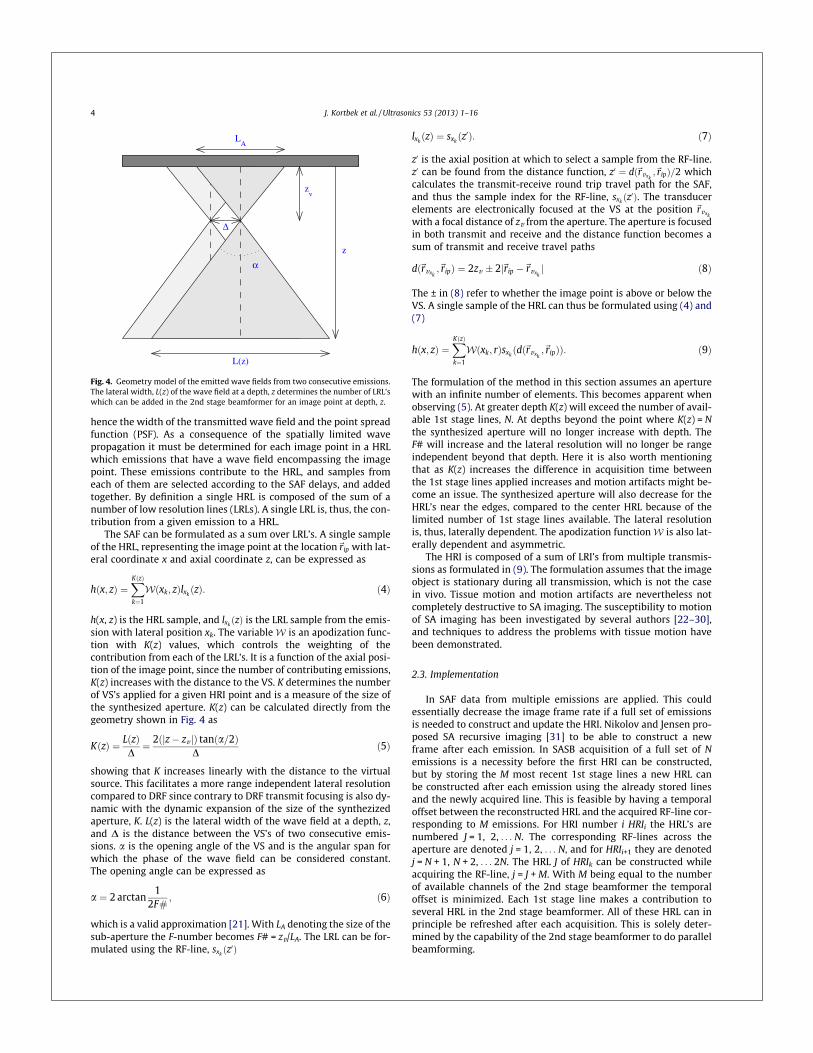
hence the width of the transmitted wave field and the point spreadfunction (PSF). As a consequence of the spatially limited wavepropagation it must be determined for each image point in a HRLwhich emissions that have a wave field encompassing the imagepoint. These emissions contribute to the HRL, and samples fromeach of them are selected according to the SAF delays, and addedtogether. By definition a single HRL is composed of the sum of anumber of low resolution lines (LRLs). A single LRL is, thus, the con-tribution from a given emission to a HRL.

The SAF can be formulated as a sum over LRL’s. A single sampleof the HRL, representing the image point at the location~rip with lat-eral coordinate x and axial coordinate z, can be expressed as

hðx; zÞ ¼XKðzÞk¼1

Wðxk; zÞlxkðzÞ: ð4Þ

h(x, z) is the HRL sample, and lxkðzÞ is the LRL sample from the emis-

sion with lateral position xk. The variableW is an apodization func-tion with K(z) values, which controls the weighting of thecontribution from each of the LRL’s. It is a function of the axial posi-tion of the image point, since the number of contributing emissions,K(z) increases with the distance to the VS. K determines the numberof VS’s applied for a given HRI point and is a measure of the size ofthe synthesized aperture. K(z) can be calculated directly from thegeometry shown in Fig. 4 as

KðzÞ ¼ LðzÞD¼ 2ðjz� zv jÞ tanða=2Þ

Dð5Þ

showing that K increases linearly with the distance to the virtualsource. This facilitates a more range independent lateral resolutioncompared to DRF since contrary to DRF transmit focusing is also dy-namic with the dynamic expansion of the size of the synthezizedaperture, K. L(z) is the lateral width of the wave field at a depth, z,and D is the distance between the VS’s of two consecutive emis-sions. a is the opening angle of the VS and is the angular span forwhich the phase of the wave field can be considered constant.The opening angle can be expressed as

a ¼ 2 arctan1

2F#; ð6Þ

which is a valid approximation [21]. With LA denoting the size of thesub-aperture the F-number becomes F# = zv/LA. The LRL can be for-mulated using the RF-line, sxk

ðz0Þ

lxkðzÞ ¼ sxk

ðz0Þ: ð7Þ

z0 is the axial position at which to select a sample from the RF-line.z0 can be found from the distance function, z0 ¼ dð~rvxk

;~ripÞ=2 whichcalculates the transmit-receive round trip travel path for the SAF,and thus the sample index for the RF-line, sxk

ðz0Þ. The transducerelements are electronically focused at the VS at the position ~rvxk

with a focal distance of zv from the aperture. The aperture is focusedin both transmit and receive and the distance function becomes asum of transmit and receive travel paths

dð~rvxk;~ripÞ ¼ 2zv � 2j~rip �~rvxk

j ð8Þ

The ± in (8) refer to whether the image point is above or below theVS. A single sample of the HRL can thus be formulated using (4) and(7)

hðx; zÞ ¼XKðzÞk¼1

Wðxk; rÞsxkðdð~rvxk

;~ripÞÞ: ð9Þ

The formulation of the method in this section assumes an aperturewith an infinite number of elements. This becomes apparent whenobserving (5). At greater depth K(z) will exceed the number of avail-able 1st stage lines, N. At depths beyond the point where K(z) = Nthe synthesized aperture will no longer increase with depth. TheF# will increase and the lateral resolution will no longer be rangeindependent beyond that depth. Here it is also worth mentioningthat as K(z) increases the difference in acquisition time betweenthe 1st stage lines applied increases and motion artifacts might be-come an issue. The synthesized aperture will also decrease for theHRL’s near the edges, compared to the center HRL because of thelimited number of 1st stage lines available. The lateral resolutionis, thus, laterally dependent. The apodization functionW is also lat-erally dependent and asymmetric.

The HRI is composed of a sum of LRI’s from multiple transmis-sions as formulated in (9). The formulation assumes that the imageobject is stationary during all transmission, which is not the casein vivo. Tissue motion and motion artifacts are nevertheless notcompletely destructive to SA imaging. The susceptibility to motionof SA imaging has been investigated by several authors [22–30],and techniques to address the problems with tissue motion havebeen demonstrated.

2.3. Implementation

In SAF data from multiple emissions are applied. This couldessentially decrease the image frame rate if a full set of emissionsis needed to construct and update the HRI. Nikolov and Jensen pro-posed SA recursive imaging [31] to be able to construct a newframe after each emission. In SASB acquisition of a full set of Nemissions is a necessity before the first HRI can be constructed,but by storing the M most recent 1st stage lines a new HRL canbe constructed after each emission using the already stored linesand the newly acquired line. This is feasible by having a temporaloffset between the reconstructed HRL and the acquired RF-line cor-responding to M emissions. For HRI number i HRIi the HRL’s arenumbered J = 1, 2, . . . N. The corresponding RF-lines across theaperture are denoted j = 1, 2, . . . N, and for HRIi+1 they are denotedj = N + 1, N + 2, . . . 2N. The HRL J of HRIk can be constructed whileacquiring the RF-line, j = J + M. With M being equal to the numberof available channels of the 2nd stage beamformer the temporaloffset is minimized. Each 1st stage line makes a contribution toseveral HRL in the 2nd stage beamformer. All of these HRL can inprinciple be refreshed after each acquisition. This is solely deter-mined by the capability of the 2nd stage beamformer to do parallelbeamforming.

L(z)

zv

z

Δ

LA

α

Fig. 4. Geometry model of the emitted wave fields from two consecutive emissions.The lateral width, L(z) of the wave field at a depth, z determines the number of LRL’swhich can be added in the 2nd stage beamformer for an image point at depth, z.


A view on implementation of the SASB at a block function leveldemonstrates a requirement for two beamformers and memory forstorage of the 1st stage image lines to feed the 2nd stage beam-former. The 1st stage beamformer is simple since the receive de-lay-profiles are the same for all image points except for a depthdependent additive constant. It only requires calculation of a singleprofile or a look up table (LUT) with a single entry. It could easily beanalog and thereby save many ADC’s. The 2nd stage beamformerhas the complexity of a general dynamic receive focusing beam-former. For each depth a separate entry in a LUT for a profile is re-quired or the delay profile must be calculated. Apodization is also adesirable requirement for the 2nd stage beamformer to suppressoff-axis energy lobes. Since K(z) increases linearly with depth theapodization is dynamic. The apodization is also a function of thelateral position of the HRL due to the finite aperture and it canprofitably be calculated as a parametric function. The desired num-ber of channels of a single-beam beamformer in the 2nd stageequals the number of acquired 1st stage lines to synthesize the fullsize array. The channel count, C of the 2nd stage beamformer canbe reduced though with a factor of M to C = N/M using a M-beambeamformer capable of processing M parallel beams and an addi-tional accumulation buffer for temporary output lines. In this formand in a case of N 1st stage lines (N acquisitions) and N 2nd stagelines the 2nd stage temporary output lines of the beamformer areLout = mod ([0: (M � 1)]C + n � 1, N) + 1 using the 1st stage lines forthe input of the beamformer Lin = mod ([0: (C � 1)] + n � 1, N) + 1for beamforming operation n. After N operations each output linehas been generated M times using M different sets of input signals(different virtual sources). By accumulating the M temporary out-put lines in the buffer the resulting output lines are exactly thesame as if a single-beam N-channel beamformer is used.

3. Simulation results

In this section the method is investigated using simulations inField II [18,19] and SAF is carried out using the BeamformationToolbox, BFT2 [20]. Images of point targets using different realiza-tions of SASB are created. The axial and lateral resolution are ex-tracted and compared to conventional B-mode imaging. Thesimulations are made with a model of a linear array 7 MHz trans-ducer with properties similar to a commercial transducer.

3.1. Setup

The parameters, which are the most decisive for the perfor-mance of SASB are the focal depth zv (the focal depth), and theF# of the VS. A parameter study is done by varying zv with valuesof 5, 10, 15, 20 mm, and the F# with values in the range 0.5–2.5.The study is done with a default set of transducer parametersand processing parameters shown in Table 1.

In the main parameter study the value of Ne = 401 has been setto exclude the effects of a finite aperture to demonstrate the abilityof the method to generate a range independent resolution. Thenumber of 1st stage image lines and also 2nd stage image lines isthe same as the number of transducer elements.

In this study a single cycle sinusoid is used as excitation and aweighted double cycle sinusoid is used to simulate the transducerimpulse response. Another less extensive study is performed withmore practical realizable parameters. The number of elements isN = 191. A double cycle sinusoid forms the excitation, and the mea-sured impulse response of the applied transducer type is used. Thescattering media consists of stationary point targets (PTs) placed inthe center of the image in the range from 5 mm to 95 mm with adistance of 10 mm.

3.2. Resolution study

Different realizations of SASB are simulated to evaluate perfor-mance and limitations. The position of the VS and the opening an-gle determines the image area covered by a single emission. If thecovered area increases, the number of 1st stage lines, which can beused for the 2nd stage beamforming, also increases, yielding a lar-ger synthesized aperture. This explicitly sets demands on the sizeof the array and the number of required 2nd stage beamformerchannels if a range independent resolution is the objective. Thestudy will show that other complications exist with the combina-tion of a shallow focal depth and a large opening angle.

The log compressed envelope HRI’s are shown in this section.The axial and lateral resolution are extracted at the image centerfor several depths. The resolution is quantified at �6 dB, the FullWidth at Half Maximum (FWHM), and at �40 dB. For each PT the

Table 1Default values for the simulation parameter study.

Parameter Value

VariousSampling frequency fs 120 MHzTransducerPitch D 0.208 mmCenter frequency fc 7 MHzBandwidth, relative B 0.6Elevation focus zele 25 mmNumber of elements N 401Excitation 1 Cycle sinusoid1st Stage processingFocusing Fixed, (xmt/rcv)Number of channels, xmt/rcv N1st 63/63Transmit sub-aperture Symmetric onlyTransmit apodization Axmt HammingFocal depth (virtual source) zv 5, 10, 15, 20 mmReceive apodization Arcv HammingReceive sub-aperture Same as transmitNumber of image lines N 401Distance between lines D 0.208 mm2nd Stage processingFocusing Synthetic apertureNumber of channels N2nd 401SA weighting W HammingNumber of image lines N 401Distance between lines D 0.208 mmApplied 1st stage lines Symmetric only

−20 0 20

0

20

40

60

80

100

axia

l [m

m]

lateral [mm]

F#=0.5

−20 0 20

0

20

40

60

80

100

lateral [mm]

F#=2

Fig. 5. Contour plots of the envelope of the output from the 1st stage beamformer.F# = 0.5 (left), and F# = 2 (right). The VS is at 5 mm. The curvature of the PSF isdetermined by the distance between the VS’s and the point of the PSF. This iscalculated analytically and shown as dotted lines for two points just above andbelow the PT at z = 65 mm.


resolution is calculated as the width at which the envelope ampli-tude has decreased to the specified level relative to the maximumlevel at that given PT. For the lateral resolution the envelopeamplitude is taken as the maximum amplitude within a axial rangeof ±3 mm around the PT. Likewise for the axial resolution theenvelope amplitude is taken as the maximum amplitude acrossthe entire lateral range of the image.

A poor lateral resolution is the consequence of having a PSFwith a wide main lobe and/or high side-lobe levels. The illustra-tions of the quantified lateral resolution reflects this by also show-ing the main-lobe resolution as a dotted line, but only if the lateralPSF has a distinct main-lobe and side-lobe distribution. That is if

the lateral PSF drops below the � 40 dB level and rises above thislevel again at a greater lateral position.

axia

l [m

m]

lateral [mm]

F#=0.5

−20 0 20

0

20

40

60

80

100

lateral [mm]

F#=1

−20 0 20

0

20

40

60

80

100

lateral [mm]

F#=1.5

−20 0 20

0

20

40

60

80

100

lateral [mm]

F#=2

−20 0 20

0

20

40

60

80

100

Fig. 6. SASB Images with the VS at 5 mm and with different values of F#. Dynamic Range is 60 dB.

0 20 40 60 80 1000

0.2

0.4

0.6

0.8

Depth [mm]

[mm

]

Lateral Resolution. Att.level −6dB

0 20 40 60 80 1000

0.02

0.04

0.06

0.08

0.1

0.12

0.14

Depth [mm]

[mm

]Axial Resolution. Att.level −6dB

F=0.5F=1.0F=1.5F=2.0

0 20 40 60 80 1000

5

10

15

20

25

Depth [mm]

[mm

]


0 20 40 60 80 1000

0.5

1

1.5

2

2.5

3

Depth [mm]

[mm

]

Axial Resolution. Att.level −40dB

Fig. 7. Resolution as function of depth at �6 dB (top) and �40 dB (bottom). Lateral resolution (left) and axial resolution (right). If the lateral PSF has a distinct main-lobe andside-lobe distribution, the main-lobe resolution is shown as a dotted line. Shown for the four different setups represented in Fig. 6.

x [mm]

z [m

m]

−20 −15 −10 −5 0 5 10 15 20

12141618

Fig. 8. A zoom in on the HRI shown in Fig. 6 for F# = 0.5. Three different HRL’s aremarked with dotted lines. The LRL’s composing these HRL’s are shown in Figs. 9–11.


z [m

m]

LRL

−5 0 5

14.5

15

15.5−1 0 1

Norm. Σ LRL

x [mm] & VS#

z [m

m]

Weighted LRL (WLRL)

160 180 200 220 240

14.5

15

15.5−1 0 1

Norm. Σ WLRL

−60 −40 −20 0dB

Env. Rel. to HRImax

Fig. 9. The LRL’s composing the center HRL of the HRI shown in Fig. 8. The LRL’s are shown before and after the weighting function. The summation of the LRL’s and thecorresponding envelope are also shown.

z [m

m]

LRL

−20 −10 0 10 20

12

14

16

18−1 0 1

Norm. Σ LRL

x [mm]

z [m

m]

Zoom on WLRL

0 1 2 3

14.8

14.9

15

15.1

15.2−1 0 1

Norm. Σ WLRL

−60 −40 −20 0dB

Env. Rel. to HRImax

Fig. 10. The LRL’s composing the off-center HRL at the lateral position x = 3.1 of the HRI shown in Fig. 8. A zoom in on a few of the weighted LRL’s is shown to visualizedestructive summation of the LRL’s.


The PSF at the output of the 1st stage beamformer has a largeextent because of the fixed receive focusing. The curvature is deter-mined by the distance between the VS’s and the point of the PSF.Consider the point at position ~rp ¼ ðx; zÞ ¼ ð0; zpÞ. The curvature,zc(x) is

zcðnÞ ¼ zv �ffiffiffiffiffiffiffiffiffiffiffiffiffiffiffiffiffiffiffiffiffiffiffiffiffiffiffiffiffiffiffiffiffiffiffiffiffiffiffiffiffiðzp � zvÞ2 þ ðjnjDÞ2

q: ð10Þ

The variable x has been substituted by nD, where �N/2 6 n 6 N/2 isthe VS number counting from the VS at x = 0. The ± refer to whetherthe image point is above or below the VS, just as in (3), and (8). Thecontour plot of the PSF is shown in Fig. 5 with a VS at 5 mm and

with F# = 0.5, and F# = 2. The shape of the PSF is the same in bothcases, but the width of the PSF differs due to the different openingangles. zc(n) from (10) has been plotted on top of the contour plot toillustrate the coherence. A PT is placed at z = 65 mm and zc has beenplotted for two points at zp = 64 mm and zp = 66 mm, respectively.The curvatures of these plots are similar to the PSF.

The envelope images after 2nd stage processing of these datasets are shown in Fig. 6 with a 60 dB dynamic range. The imagesare constructed with N = 401 which equals an image width ofapproximately 83 mm, but the displayed images have beencropped to a width of 40 mm. The resolution seems range indepen-dent if the dominant side-lobes are discounted. The lateral

z [m

m]

LRL

−20 −10 0 10 20

12

14

16

18−1 0 1

Norm. Σ LRL

x [mm]

z [m

m]

Zoom on WLRL

2.5 3 3.5 4

14.7

14.8

14.9

15

15.1

15.2

−1 0 1

Norm. Σ WLRL

−60 −40 −20 0dB

Env. Rel. to HRImax

Fig. 11. The LRL’s composing the off-center HRL at the lateral position x = 6.7 of the HRI shown in Fig. 8. A zoom in on a few of the weighted LRL’s is shown to visualize aphase-shift of almost an entire pulse-echo wave length, yielding undesired constructive summation, and an envelope level above �40 dB.

axia

l [m

m]

lateral [mm]

Pitch=λ

−20 −10 0 10 20

0

5

10

15

20

25

30

35

40

45

lateral [mm]

Pitch=λ/2

−20 −10 0 10 20

0

5

10

15

20

25

30

35

40

45

Fig. 12. Two SASB images are constructed using a linear array (left) and a linear phased array (right). Both having 401 elements, a VS at 5 mm, and with F# = 0.75. The lineararray is twice the width of the phased array, but the image has been cropped to the same width as the phased array image. Dynamic range is 70 dB.


resolution decreases as the F# increases as expected because of thedecrease in the width of the synthesized aperture.

The quantified resolution of the HRI in Fig. 6 is shown in Fig. 7.The resolution is practically constant at �6 dB and �40 dB throughrange for all values of F#, with a few exceptions. The exceptions arefor those PT near the VS when F# = 0.5. Here the side-lobe level isvery dominant. Side-lobes are also noticeable for F# = 1 when look-ing at the HRI in Fig. 6. They are below the �40 dB level though anddo not show in Fig. 7.

3.2.1. Investigating grating-lobesThe off-axis energy-lobes in Fig. 6 for F# = 0.5 are dominant.

Taking a closer look at the phase of those LRL’s which are summedin the 2nd stage beamformer can disclose the origin of this artifact.The part of the image containing the PT at 15 mm is shown inFig. 8. Three different HRL’s are investigated. They are marked withdotted lines in Fig. 8. SASB relies on phase coherent addition of theLRL’s as expressed in (4). The LRL’s composing the center HRL areplotted in Fig. 9. It is apparent that the LRL’s are completely phasealigned and add up constructively as expected. The figure showsthe LRL’s before and after the weighting function. It also showsthe HRL, hence the summation of the LRL’s and the correspondingenvelope. Finally the envelope of the weighted HRL is shown rela-tive to the maximum of the HRI in Fig. 8.

The LRL’s composing the HRL at x = 3.1 mm are plotted inFig. 10. The LRL’s are shown before the weighting and a zoom inon a few of the LRL’s after the weighting function is shown. Thephase shift between consecutive LRL’s is close to half a pulse-echowave length and this destructive summation yields an envelope le-vel near �60 dB.

The LRL’s composing the HRL at x = 6.7 mm are plotted inFig. 11. The phase shift between consecutive LRL’s has increasedto almost an entire pulse-echo wave length and the LRL’s add upconstructively to an envelope level above �40 dB. In this simulatedsetup the pulse-echo signal consists of only a few periods, henceonly a few non-zero contributions are included in the summationof the LRL’s. If the pulse-echo signal contains several periods

several non-zero LRL’s will be present in the sum, yielding an evenhigher envelope level.

The artifacts shown are grating lobes, since they arise due to lat-eral spatial under-sampling. Consider having a setup with a phasedarray transducer with a k/2 pitch and, thus, twice the lateral den-sity of VS’s. The illustration of LRL’s prior to summation equivalentto the one shown in Fig. 11 will contain LRL’s with a phase shiftbetween consecutive LRL’s of only half a wave length. Every secondLRL will be equal to the ones shown in Fig. 11 but every other LRLwill have a phase which is in between the two. The result isdestructive summation instead of unintentional constructive sum-mation, and the massive grating lobes are avoided. This is exempli-fied in Fig. 12. Two HRI’s are constructed using a linear array withk-pitch and a linear phased array with k/2-pitch respectively. The

VS

HRL

θr

z [m

m]

x [mm]

LRLs for the HRL at x=5 mm

circle with radius zr, and center at VS

−10 −5 0 5 10

0

2

4

6

8

10

12

14

16

18

Fig. 13. The log-compressed envelope of the LRL’s constituting the HRL atxh = 4 mm is shown in the range 12–18 mm with a dynamic range of 50 dB. TheVS is at the depth zv = 5 mm and F# = 0.5. A PT is positioned at the point~rp ¼ ðx; yÞ ¼ ð0; zpÞ with depth, zp = 15 mm. The appearance of the LRL’s for the off-center HRL can be approximated by a rotation of the LRL’s of the center HRL. Thecenter of rotation is the VS of the off-center HRL, and the rotation radius iszr = zp � zv. The angle of rotation hr = arcsin (xh/zr) is also indicated.

0 20 40 60 80 1000

0.2

0.4

0.6

0.8

[mm

]


0 20 40 60 80 1000

2

4

6

8

Depth [mm]

[mm

]Lateral Resolution. Att.level −40dB

VS@5mmVS@10mmVS@15mmVS@20mm

Fig. 14. Lateral resolution with F# = 1.5 as a function of depth at �6 dB (top) and�40 dB (bottom).

axia

l [m

m]

lateral [mm]

N=401, Short PE

−20 0 20

0

10

20

30

40

50

60

70

80

90

100

lateral [mm]

N=191, Long PE

−20 0 20

0

10

20

30

40

50

60

70

80

90

100

Fig. 15. Envelope images with the VS at 20 mm and with F# = 2. Two differentsimulation models are used. N = 401, and a short pulse-echo (PE) response (left).N = 191, and a long pulse-echo response (right). The image using N = 401 has beencropped to the same width as the image using N = 191. Dynamic range is 60 dB.


difference between the two images is striking, since the gratinglobes are avoided by increasing the lateral spatial sampling inthe 1st stage processing.

The VS’s can be conceived as elements in a virtual array. In SASBthe wave fields from several emissions are sampled by the virtualarray and coherently added. For a given frequency grating lobesarise at a combination of a sparse spatial sampling by the virtualarray and wave fields with incident angles beyond a certain limit.Both of these parameters can be controlled in SASB to prevent grat-ing lobes. The array spacing and the VS spacing do not have to bethe same. With a dense lateral sampling the VS can have k/2 spac-ing even though the array has k spacing. For a given spacing be-tween the VS’s the range of incident angles must be restricted.This is possible by putting a limit to the opening angle of the VS.

The restriction on the opening angle to avoid grating lobes canbe demonstrated from an analysis of the LRL’s constituting the off-center HRL’s. In Fig. 9 the LRL’s constituting the center HRL arephase-coherently aligned. They are aligned at the depth,zp = 15 mm, where a PT at ~rp ¼ ðx; yÞ ¼ ð0; zpÞ is placed. In Fig. 11the LRL’s constituting an off-center HRL at the lateral position xh

are no longer aligned phase-coherently. As a simple approximationthese LRL’s can be found by a rotation of the aligned LRL’s. The lineof phase equality is perpendicular to the line with origin in the VSof the off-center HRL and going to ~rp and with length zr = zp � zv,where zv is the depth of the VS. The angle of this line is

hr ¼ arcsinxh

zr

� �: ð11Þ

This geometry is illustrated in Fig. 13 superimposed on the log-compressed envelope of a set of LRL’s from the HRL at xh = 5 mm.The exact positions of constant phase are also indicated in Fig. 13as a dashed line. It comes from the intersections of the indices

representing the PT and the indices representing a number of FP’sall placed in the same off-center HRL.

By applying the approximation about the rotated LRL’s it is pos-sible to estimate the phase shift between consecutive LRL’s with asimple expression. The axial shift between consecutive LRL’s is

x ¼ tan hrD: ð12Þ

Substituting hr with half the opening angle, a0 = a/2 the axial shiftcan be expressed as

x ¼ tanða0ÞD ¼ D2F#

: ð13Þ

If the spatial shift does not exceed half the wavelength of the pulse-echo signal, kpe = k/2 = c/f0/2 grating lobes are avoided. That is

0 20 40 60 80 1000

0.2

0.4

0.6

0.8

1

Depth [mm]

[mm

]


N=401, Short PEN=191, Long PE

0 20 40 60 80 1000

0.1

0.2

0.3

0.4

0.5

Depth [mm]

[mm

]


0 20 40 60 80 1000

2

4

6

8

Depth [mm]

[mm

]


0 20 40 60 80 1000

0.5

1

1.5

Depth [mm]

[mm

]


Fig. 16. Resolution as function of depth at�6 dB (top) and�40 dB (bottom). Lateral resolution (left) and axial resolution (right). If the lateral PSF has a distinct main-lobe, andside-lobe distribution, the main-lobe resolution is shown as a dotted line. The resolution is extracted from the HRI’s in Fig. 15.

x [mm]

z [m

m]

−10 −8 −6 −4 −2 0 2 4 6 8 10

5354555657

x [mm]

z [m

m]

−10 −8 −6 −4 −2 0 2 4 6 8 10

5354555657

Fig. 17. Envelope images with the VS at 10 mm, and with F# = 2 from Fig. 15. ShortPE response (top), and long PE response (bottom). Shown in the range from 53 mmto 57 mm, and superimposed with vertical dashed lines indicating those HRL’s forwhich the LRL’s are shown. The LRL’s are shown in Figs. 18 and 19.


x < kpe/2 or x < k/4 This condition can be used to put restrictions onthe F# of the VS

F# PD

k=2for x 6 k=4: ð14Þ

The opening angle of the VS limits the range of angles of the wavefield. If a transducer with D = k is used in SASB grating lobes areavoided if F# P 2.

The spatial pulse-echo wavelength is extracted from the centerLRL and is kpe = 0.15 mm. With D = 0.208 mm the VS must be de-signed with F# P 1.39 with the restriction of (14). This is alsoreflected in Fig. 6, where the grating lobes evidently are attenuatedfor F# = 1.5 and F# = 2 compared to the setup where F# = 0.5, andF# = 1. In Fig. 12 (right) a phased array with pitch D = 0.104 is ap-plied, which requires F# P 0.70. The applied F# is 0.75 and thegrating lobes are avoided. Notice that the requirement for the F#is not tied to the array spacing but to the spacing of the VS’s. The

z [m

m]

Weighted LRL (WLRL)

−10 −5 0 5 10

54.4

54.6

54.8

55

55.2

55.4

55.6

−1 0 1

Norm. Σ WLRL

−60 −40 −20 0

Env. Rel. to HRImax

x [mm]

z [m

m]

Weighted LRL (WLRL)

−10 −5 0 5 10

54.4

54.6

54.8

55

55.2

55.4

55.6

−1 0 1

Norm. Σ WLRL

−60 −40 −20 0dB

Env. Rel. to HRImax

Fig. 18. The LRL’s composing the center HRL of the two HRI’s shown in Fig. 17. The LRL’s are shown after the weighting function. The summation of the LRL’s and thecorresponding envelope are also shown.


setup is thus equivalent to a setup where D = 0.208 and the densityof the VS’s is doubled.

K(z) from (5) determines the number of VS’s applied and thesize of the synthesized aperture. It is a function of the position ofthe VS and the opening angle and, thus, the F#. It was shown pre-viously that the grating lobes were appropriately attenuated forthe linear array with F# = 1.5 when the VS was at 5 mm. The lateralresolution with F# = 1.5 and different positions of the VS is shown

z [m

m]

Weighted LRL (WLRL)

−10 −5 0 5 10

54.4

54.6

54.8

55

55.2

55.4

55.6

−1 0 1

Norm. Σ WLRL

−60 −40 −20 0

Env. Rel. to HRImax

x [mm]

z [m

m]

Weighted LRL (WLRL)

−10 −5 0 5 10

54.4

54.6

54.8

55

55.2

55.4

55.6

−1 0 1

Norm. Σ WLRL

−60 −40 −20 0dB

Env. Rel. to HRImax

Fig. 19. The LRL’s composing the off-center HRL of the two HRI’s shown in Fig. 17. The LRL’s are shown after the weighting function. The summation of the LRL’s and thecorresponding envelope are also shown.

Table 2The number of array elements used during transmission as a function of VS positionand F#.

VS depth F# = 1.5 F# = 2

5 mm 17 1310 mm 33 2515 mm 49 3720 mm 65 49


in Fig. 14. The resolution functions are very similar but not thesame in the four different setups because of the different numberof applied VS’s.

3.2.2. Influence of transducer impulse responseThe performance results presented in the previous sections

were based on a transducer with N = 401, a short excitation signal,and a simple impulse response. The performance using a morerealistic transducer simulation model is presented in this sectionand a comparison between the two is made. Envelope images withthe VS at 20 mm, F# = 2, and with the two different simulationmodels are shown in Fig. 15. The new simulation model hasN = 191. The excitation signal has two periods, and the impulse re-sponse is the measured response of a commercial transducer yield-ing a longer pulse-echo (PE) response. The difference between thetwo images is significant. The axial resolution has decreased as aconsequence of the extended PE response. The lateral resolutionhas improved in the entire range also beyond depths of 80 mm,where K(z) ceases to increase linearly. The axial and lateral resolu-tion are extracted, and shown in Fig. 16. The improvement in lat-eral resolution at �40 dB is at least a factor of 2.

To illustrate the cause of the difference in performance, theLRL’s composing the HRI’s are investigated. The investigation

concerns only the range from 53 mm to 57 mm which include asingle PT at a depth of 55 mm. The HRI’s in this range are shownin Fig. 17, superimposed with vertical dashed lines indicating thoseHRL’s for which the LRL’s are shown.

The LRL’s for the center HRL are shown in Fig. 18. The LRL’s forthe off-center HRL are shown in Fig. 19. In these figures the LRL’safter LRL-weighting are shown. They also show the summation ofthe LRL’s and the corresponding envelope. Finally the envelope ofthe weighted HRL is shown relative to the maximum of the HRI’sin Fig. 17. The LRL’s sum completely constructive for the centerHRL in both setups.

For the off-center HRL’s the LRL’s sum destructively toward zerolevel. With a short pulse-echo response the off-center HRL is com-posed of the sum of a only a few positive and negative half-periods.The amplitudes of these half-periods varies with range and lateralposition. The amplitude of the HRL, thus, varies with range. Thevariation over range is considerable due to the sparse number ofcycles in the sum.

With a longer pulse-echo response the off-center HRL is com-posed of the sum of several positive and negative half-periods.The amplitudes of these half-periods decay smoothly over rangeand lateral position and on average sum destructively to a zero le-vel. The HRL is of oscillating nature with the same center frequencyas the pulse-echo response, which is not the case for the setup withthe short PE response.

3.2.3. Comparison to dynamic receive focusingThe performance of SASB is among others a function of VS posi-

tion and F#. These parameters also determine the number of ele-ments used during transmission. This has an influences on theemitted energy and the signal to noise ratio. It was shown in Sec-tion 3.2.1 that the grating lobes were appropriately attenuated forF# = 1.5 and F# = 2. The number of elements used as a function ofVS position and F# is shown in Table 2.

The choice of configuration for comparison with DRF is based onthe results presented in Fig. 20. Here the lateral resolution for anumber of configurations is shown. In all configurations the resultsare based on the realistic transducer simulation model introduced

0 20 40 60 80 1000

0.1

0.2

0.3

0.4

0.5

0.6

0.7

0.8

Depth [mm]

[mm

]


VS@10, F=1.5VS@15, F=1.5VS@20, F=1.5VS@10, F=2.0VS@15, F=2.0VS@20, F=2.0

0 20 40 60 80 1000

0.5

1

1.5

2

2.5

3

3.5

4

4.5

Depth [mm]

[mm

]


Fig. 20. Lateral resolution of SASB as function of depth at �6 dB (top) and �40 dB(bottom). If the lateral PSF has a distinct main-lobe, and side-lobe distribution, themain-lobe resolution is shown as a dotted line. In all configurations the results arebased on the realistic transducer simulation model introduced in Section 3.2.2.

axia

l [m

m]

lateral [mm]

DRF

−20 0 20

0

10

20

30

40

50

60

70

80

90

100

lateral [mm]

SASB

−20 0 20

0

10

20

30

40

50

60

70

80

90

100

Fig. 21. Envelope images using DRF (left) and SASB (right). For DRF the transmitfocal point is at 70 mm. For SASB the VS is at 20 mm and F# = 1.5. Dynamic Range is60 dB.


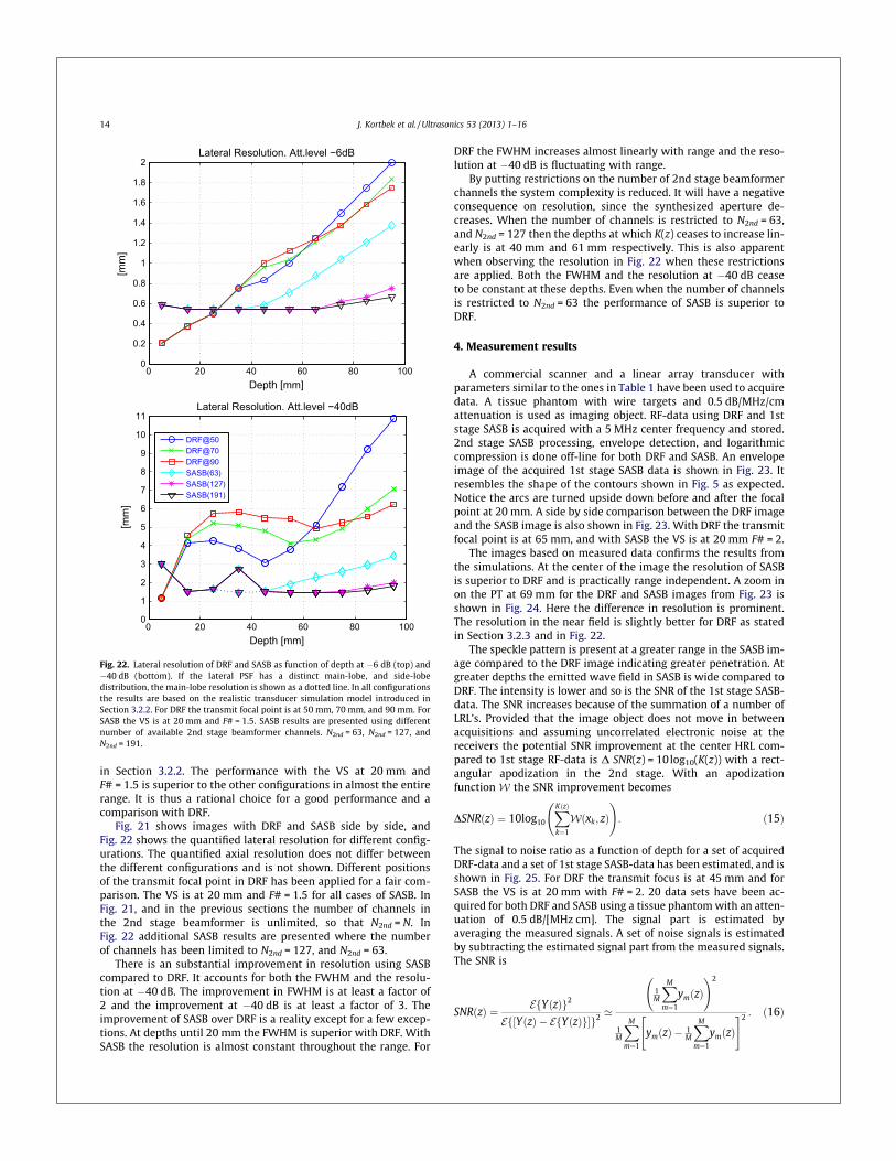
in Section 3.2.2. The performance with the VS at 20 mm andF# = 1.5 is superior to the other configurations in almost the entirerange. It is thus a rational choice for a good performance and acomparison with DRF.

Fig. 21 shows images with DRF and SASB side by side, andFig. 22 shows the quantified lateral resolution for different config-urations. The quantified axial resolution does not differ betweenthe different configurations and is not shown. Different positionsof the transmit focal point in DRF has been applied for a fair com-parison. The VS is at 20 mm and F# = 1.5 for all cases of SASB. InFig. 21, and in the previous sections the number of channels inthe 2nd stage beamformer is unlimited, so that N2nd = N. InFig. 22 additional SASB results are presented where the numberof channels has been limited to N2nd = 127, and N2nd = 63.

There is an substantial improvement in resolution using SASBcompared to DRF. It accounts for both the FWHM and the resolu-tion at �40 dB. The improvement in FWHM is at least a factor of2 and the improvement at �40 dB is at least a factor of 3. Theimprovement of SASB over DRF is a reality except for a few excep-tions. At depths until 20 mm the FWHM is superior with DRF. WithSASB the resolution is almost constant throughout the range. For

DRF the FWHM increases almost linearly with range and the reso-lution at �40 dB is fluctuating with range.

By putting restrictions on the number of 2nd stage beamformerchannels the system complexity is reduced. It will have a negativeconsequence on resolution, since the synthesized aperture de-creases. When the number of channels is restricted to N2nd = 63,and N2nd = 127 then the depths at which K(z) ceases to increase lin-early is at 40 mm and 61 mm respectively. This is also apparentwhen observing the resolution in Fig. 22 when these restrictionsare applied. Both the FWHM and the resolution at �40 dB ceaseto be constant at these depths. Even when the number of channelsis restricted to N2nd = 63 the performance of SASB is superior toDRF.

4. Measurement results

A commercial scanner and a linear array transducer withparameters similar to the ones in Table 1 have been used to acquiredata. A tissue phantom with wire targets and 0.5 dB/MHz/cmattenuation is used as imaging object. RF-data using DRF and 1ststage SASB is acquired with a 5 MHz center frequency and stored.2nd stage SASB processing, envelope detection, and logarithmiccompression is done off-line for both DRF and SASB. An envelopeimage of the acquired 1st stage SASB data is shown in Fig. 23. Itresembles the shape of the contours shown in Fig. 5 as expected.Notice the arcs are turned upside down before and after the focalpoint at 20 mm. A side by side comparison between the DRF imageand the SASB image is also shown in Fig. 23. With DRF the transmitfocal point is at 65 mm, and with SASB the VS is at 20 mm F# = 2.

The images based on measured data confirms the results fromthe simulations. At the center of the image the resolution of SASBis superior to DRF and is practically range independent. A zoom inon the PT at 69 mm for the DRF and SASB images from Fig. 23 isshown in Fig. 24. Here the difference in resolution is prominent.The resolution in the near field is slightly better for DRF as statedin Section 3.2.3 and in Fig. 22.

The speckle pattern is present at a greater range in the SASB im-age compared to the DRF image indicating greater penetration. Atgreater depths the emitted wave field in SASB is wide compared toDRF. The intensity is lower and so is the SNR of the 1st stage SASB-data. The SNR increases because of the summation of a number ofLRL’s. Provided that the image object does not move in betweenacquisitions and assuming uncorrelated electronic noise at thereceivers the potential SNR improvement at the center HRL com-pared to 1st stage RF-data is D SNR(z) = 10log10(K(z)) with a rect-angular apodization in the 2nd stage. With an apodizationfunction W the SNR improvement becomes

DSNRðzÞ ¼ 10log10

XKðzÞk¼1

Wðxk; zÞ !

: ð15Þ

The signal to noise ratio as a function of depth for a set of acquiredDRF-data and a set of 1st stage SASB-data has been estimated, and isshown in Fig. 25. For DRF the transmit focus is at 45 mm and forSASB the VS is at 20 mm with F# = 2. 20 data sets have been ac-quired for both DRF and SASB using a tissue phantom with an atten-uation of 0.5 dB/[MHz cm]. The signal part is estimated byaveraging the measured signals. A set of noise signals is estimatedby subtracting the estimated signal part from the measured signals.The SNR is

SNRðzÞ ¼ EfYðzÞg2

Ef½YðzÞ � EfYðzÞg�g2 ’

1M

XM

m¼1

ymðzÞ !2

1M

XM

m¼1

ymðzÞ � 1M

XM

m¼1

ymðzÞ" #2 : ð16Þ

0 20 40 60 80 1000

0.2

0.4

0.6

0.8

1

1.2

1.4

1.6

1.8

2

Depth [mm]

[mm

]


0 20 40 60 80 1000

1

2

3

4

5

6

7

8

9

10

11

Depth [mm]

[mm

]


DRF@50DRF@70DRF@90SASB(63)SASB(127)SASB(191)

Fig. 22. Lateral resolution of DRF and SASB as function of depth at �6 dB (top) and�40 dB (bottom). If the lateral PSF has a distinct main-lobe, and side-lobedistribution, the main-lobe resolution is shown as a dotted line. In all configurationsthe results are based on the realistic transducer simulation model introduced inSection 3.2.2. For DRF the transmit focal point is at 50 mm, 70 mm, and 90 mm. ForSASB the VS is at 20 mm and F# = 1.5. SASB results are presented using differentnumber of available 2nd stage beamformer channels. N2nd = 63, N2nd = 127, andN2nd = 191.


E is the expectation operator. Y(z) denotes the M number of mea-sured data sets, and ym(z) is the m’th data set. The theoretical poten-tial SNR improvement, DSNR(z) from (15) is also shown in Fig. 25with a Hamming window as SA weighting. For z = 80 mm the valueof D SNR(z) can be calculated using (6) and (5) and is 19 dB. The po-tential SNR of the SASB is superior to DRF at the entire range and animprovement of 8 dB is realized at a depth of 80 mm.

5. Conclusion

The main motivation for SASB is to apply synthetic aperturetechniques with a restricted system complexity. The objective isto improve lateral resolution and obtain a more range independentresolution compared to conventional ultrasound imaging.

The SASB method has been investigated using simulations inField II and by off-line processing of data acquired with a commer-cial scanner. The parameters which are the most decisive for theperformance are the depth of the VS (the focal depth), and theF# of the VS. The lateral resolution increases with a decreasingF#, but grating lobes arise at a combination of a sparse spatial sam-pling by the virtual array and wave fields with incident angles

axia

l [m

m]

lateral [mm]

1st stage SASB

−10 0 10

0

10

20

30

40

50

60

70

80

90

lateral [mm]

SASB

−10 0 10

0

10

20

30

40

50

60

70

80

90

lateral [mm]

DRF

−10 0 10

0

10

20

30

40

50

60

70

80

90

Fig. 23. Envelope images using 1st stage SASB (left), SASB (center), and DRF (right). RF-data is acquired using a commercial scanner, and processing is done off-line. For DRFthe transmit focal point is at 65 mm. For SASB the VS is at 20 mm and F# = 2. Dynamic Range is 60 dB.

axia

l [m

m]

lateral [mm]

DRF

−5 0 5

66

68

70

72

lateral [mm]

SASB

−5 0 5

66

68

70

72

Fig. 24. A zoom in on the DRF and SASB images from Fig. 23.

0 20 40 60 80 100 120−10

0

10

20

30

40

50

60

z [mm]

dB

SNRDRFSASB (1st)SASB (2nd, theoretical)

Fig. 25. SNR as a function of depth. Data sets are acquired with a commercialscanner and a tissue phantom for both DRF and 1 stage SASB. The estimated SNR of2nd stage SASB is also shown.


beyond a certain limit. It is possible to restrict the range of incidentangles by putting a limit to the opening angle of the VS. For a trans-ducer with a pitch of D = k grating lobes are avoided if F# P 2. For aphased array transducer with D = k/2 grating lobes are avoided ifF# P 1.

Simulations have been done with two different pulse-echo re-sponses having different bandwidths. The performance differencebetween the two simulation models is significant. The lateral res-olution is significantly better for the simulation model with thelonger pulse-echo response and the improvement is at least a fac-tor of 2 at �40 dB.

The performance of SASB with the VS at 20 mm and F# = 1.5 iscompared with conventional dynamic receive focusing (DRF). Theaxial resolution is the same for the two methods. There is an sub-stantial improvement in lateral resolution using SASB compared toDRF. It accounts for both the FWHM and the resolution at �40 dB.The improvement in FWHM is at least a factor of 2 and theimprovement at �40 dB is at least a factor of 3. The improvementof SASB over DRF is a reality except for a few exceptions. At depthsuntil 20 mm the FWHM is superior with DRF. With SASB the reso-lution is almost constant throughout the range. For DRF the FWHMincreases almost linearly with range and the resolution at �40 dBis fluctuating with range. By putting restrictions on the numberof 2nd stage beamformer channels the system complexity is re-duced. It will have a negative consequence on resolution sincethe synthesized aperture decreases, but even when the numberof channels is restricted to N2nd = 63 the performance of SASB isstill superior to DRF.

SASB has been applied to data acquired with a commercial scan-ner and a tissue phantom with wire targets. The images confirmsthe results from the simulations. At the center of the image the res-olution of SASB is superior to DRF and is practically range indepen-dent. The resolution in the near field is slightly better for DRF. Afeasible solution could be to construct the final image by applyingDRF above the VS and SASB beyond the VS.

The speckle pattern is present at a greater range in the SASB im-age compared to the DRF image indicating greater penetration. Thesignal to noise ratio as a function of depth for a set of acquired DRF-data and a set of 1st stage SASB-data has been estimated. The the-oretical potential improvement in SNR of SASB over DRF has beenestimated based on the measured SNR data and an assumption of astationary image object, and a correct phase-alignment in the 2ndstage beamformer. The improvement is attained at the entire rangeand at a depth of 80 mm the improvement is 8 dB.

References

[1] L.J. Cutrona, W.E. Vivian, E.N. Leith, G.O. Hall, A high resolution radar combat-surveillance system, IRE Trans. Mil. Elect. MIL-5 (1961) 127–131.

[2] C.W. Sherwin, J.P. Ruina, D. Rawcliffe, Some early developments in syntheticaperture radar systems, IRE Trans. Mil. Elect. MIL-6 (1962) 111–115.

[3] J.C. Curlander, R.N. McDonough, Synthetic Aperture Radar: Systems and SignalProcessing, John Wiley & Sons Inc., 1991.

[4] M. Karaman, P.C. Li, M. O’Donnell, Synthetic aperture imaging for small scalesystems, IEEE Trans. Ultrason. Ferroelec. Freq. Contr. 42 (1995) 429–442.

[5] R.Y. Chiao, L.J. Thomas, S.D. Silverstein, Sparse array imaging with spatially-encoded transmits, in: Proc. IEEE Ultrason. Symp. 1997, pp. 1679–1682.

[6] J.T. Ylitalo, H. Ermert, Ultrasound synthetic aperture imaging: monostaticapproach, IEEE Trans. Ultrason. Ferroelec. Freq. Contr. 41 (1994) 333–339.

[7] M.H. Pedersen, K.L. Gammelmark, J.A. Jensen, In-vivo evaluation of convexarray synthetic aperture imaging, Ultrasound Med. Biol. 33 (2007) 37–47.

[8] D.K. Peterson, G.S. Kino, Real-time digital image reconstruction: a descriptionof imaging hardware and an analysis of quantization errors, IEEE Trans. Son.Ultrason. 31 (1984) 337–351.

[9] G.R. Lockwood, J.R. Talman, S.S. Brunke, Real-time 3-D ultrasound imagingusing sparse synthetic aperture beamforming, IEEE Trans. Ultrason. Ferroelec.Freq. Contr. 45 (1998) 980–988.

[10] C.R. Hazard, G.R. Lockwood, Theoretical assessment of a synthetic aperturebeamformer for real-time 3-D imaging, IEEE Trans. Ultrason. Ferroelec. Freq.Contr. 46 (1999) 972–980.

[11] M. O’Donnell, L.J. Thomas, Efficient synthetic aperture imaging from a circularaperture with possible application to catheter-based imaging, IEEE Trans.Ultrason. Ferroelec. Freq. Contr. 39 (1992) 366–380.

[12] C. Passmann, H. Ermert, A 100-MHz ultrasound imaging system fordermatologic and ophthalmologic diagnostics, IEEE Trans. Ultrason.Ferroelec. Freq. Contr. 43 (1996) 545–552.

[13] C.H. Frazier, W.D. O’Brien, Synthetic aperture techniques with a virtual sourceelement, IEEE Trans. Ultrason. Ferroelec. Freq. Contr. 45 (1998) 196–207.

[14] S.I. Nikolov, J.A. Jensen, Virtual ultrasound sources in high-resolutionultrasound imaging, in: Proc. SPIE – Progress in biomedical optics andimaging, vol. 3, 2002, pp. 395–405.

[15] S.I. Nikolov, J.A. Jensen, 3D synthetic aperture imaging using a virtual sourceelement in the elevation plane, in: Proc. IEEE Ultrason. Symp. vol. 2, 2000, pp.1743–1747.

[16] M.H. Bae, M.K. Jeong, A study of synthetic-aperture imaging with virtualsource elements in B-mode ultrasound imaging systems, IEEE Trans. Ultrason.Ferroelec. Freq. Contr. 47 (2000) 1510–1519.

[17] J. Kortbek, J.A. Jensen, K.L. Gammelmark, Synthetic aperture focusing appliedto imaging using a rotating single element transducer, in: Proc. IEEE Ultrason.Symp. 2007, pp. 1504–1507.

[18] J.A. Jensen, N.B. Svendsen, Calculation of pressure fields from arbitrarilyshaped, apodized, and excited ultrasound transducers, IEEE Trans. Ultrason.Ferroelec. Freq. Contr. 39 (1992) 262–267.

[19] J.A. Jensen, Field: a program for simulating ultrasound systems, Med. Biol. Eng.Comp. 10th Nordic-Baltic Conference on Biomedical Imaging 4(Supplement 1,Part 1) (1996b) 351–353.

[20] J. Kortbek, S.I. Nikolov, J.A. Jensen, Effective and versatile softwarebeamformation toolbox, in: Proc. SPIE – Medical Imaging – UltrasonicImaging and Signal Processsing, vol. 651319, 2007, pp. 1–10.

[21] N. Oddershede, J.A. Jensen, Effects influencing focusing in synthetic aperturevector flow imaging, IEEE Trans. Ultrason. Ferroelec. Freq. Contr. 54 (2007)1811–1825.

[22] L.F. Nock, G.E. Trahey, Synthetic receive aperture imaging with phasecorrection for motion and for tissue inhomogenities – Part I: basicprinciples, IEEE Trans. Ultrason. Ferroelec. Freq. Contr. 39 (1992) 489–495.

[23] G.E. Trahey, L.F. Nock, Synthetic receive aperture imaging with phasecorrection for motion and for tissue inhomogenities – Part II: effects of andcorrection for motion, IEEE Trans. Ultrason. Ferroelec. Freq. Contr. 39 (1992)496–501.

[24] H.S�. Bilge, M. Karaman, M. O’Donnell, Motion estimation using common spatialfrequencies in synthetic aperture imaging, in: Proc. IEEE Ultrason. Symp. 1996,pp. 1551–1554.

[25] M. Karaman, H.S�. Bilge, M. O’Donnell, Adaptive multi-element syntheticaperture imaging with motion and phase aberration correction, IEEE Trans.Ultrason. Ferroelec. Freq. Contr. 42 (1998) 1077–1087.

[26] C.R. Hazard, G.R. Lockwood, Effects of motion artifacts on a synthetic aperturebeamformer for real-time 3D ultrasound, in: Proc. IEEE Ultrason. Symp. 1999,pp. 1221–1224.

[27] J.S. Jeong, J.S. Hwang, M.H. Bae, T.K. Song, Effects and limitations of motioncompensation in synthetic aperture techniques, in: Proc. IEEE Ultrason. Symp.2000, pp. 1759 –1762.

[28] S.I. Nikolov, J.A. Jensen, K-space model of motion artifacts in synthetic transmitaperture ultrasound imaging, in: Proc. IEEE Ultrason. Symp. 2003, pp. 1824–1828.

[29] K.L. Gammelmark, J.A. Jensen, Multielement synthetic transmit apertureimaging using temporal encoding, IEEE Trans. Med. Imag. 22 (2003) 552–563.

[30] K.L. Gammelmark, J.A. Jensen, Duplex synthetic aperture imaging withtissue motion compensation, in: Proc. IEEE Ultrason. Symp. 2003, pp.1569–1573.

[31] S.I. Nikolov, K. Gammelmark, J.A. Jensen, Recursive ultrasound imaging, in:Proc. IEEE Ultrason. Symp. vol. 2, 1999, pp. 1621–1625.


110

BIBLIOGRAPHY

[1] M. E. Anderson, N. Bottenus, and G. E. Trahey. A seminar on k-space applied to medical ultrasound. Dept. ofBiomedical Engineering, Duke University, 2015.

[2] J. A. Jensen. Linear description of ultrasound imaging systems, notes for the international summer school onadvanced ultrasound imaging. Technical report, Department of Information Technology, DTU, 1999.

[3] J. A. Jensen. Imaging in medical diagnosis and therapy, volume 3, chapter Ultrasound Velocity Imaging, pages65–99. CRC Taylor and Francis Group, 2015. 2015; 3.

[4] J. A. Jensen, S. Nikolov, K. L. Gammelmark, and M. H. Pedersen. Synthetic aperture ultrasound imaging.Ultrasonics, 44:e5–e15, 2006.

[5] J. Kortbek, J. A. Jensen, and K. L. Gammelmark. Sequential beamforming for synthetic aperture imaging.Ultrasonics, 53(1):1–16, 2013.

[6] J. A. Jensen. A model for the propagation and scattering of ultrasound in tissue. J. Acoust. Soc. Am., 89:182–191, 1991.

[7] J. A. Jensen. A new calculation procedure for spatial impulse responses in ultrasound. J. Acoust. Soc. Am.,105(6):3266–3274, 1999.

[8] J. A. Jensen, D. Gandhi, and W. D. O’Brien. Ultrasound fields in an attenuating medium. In Proc. IEEEUltrason. Symp., pages 943–946, 1993.

[9] J. A. Jensen. Estimation of Blood Velocities Using Ultrasound: A Signal Processing Approach. CambridgeUniversity Press, New York, 1996.

[10] A. D. Pierce. Acoustics, An Introduction to Physical Principles and Applications. Acoustical Society of Amer-ica, New York, 1989.

[11] P. M. Morse and K. U. Ingard. Theoretical Acoustics. McGraw-Hill, New York, 1968.

[12] P. R. Stepanishen. Pulsed transmit/receive response of ultrasonic piezoelectric transducers. J. Acoust. Soc. Am.,69:1815–1827, 1981.

[13] L. E. Kinsler, A. R. Frey, A. B. Coppens, and J. V. Sanders. Fundamentals of Acoustics. John Wiley & Sons,New York, third edition, 1982.

[14] P. R. Stepanishen. Wide bandwidth near and far field transients from baffled pistons. In Proc. IEEE Ultrason.Symp., pages 113–118, 1977.

[15] L. Raade and B. Westergreen. β Mathematics handbook. Charwell-Bratt, Ltd., Kent, England, 1990.

[16] M. R. Spiegel. Mathematical handbook of formulas and tables. McGraw-Hill, New York, 1968.

111

[17] M. Arditi, F. S. Forster, and J. Hunt. Transient fields of concave annular arrays. Ultrason. Imaging, 3:37–61,1981.

[18] A. Penttinen and M. Luukkala. The impulse response and nearfield of a curved ultrasonic radiator. J. Phys. D:Appl. Phys., 9:1547–1557, 1976.

[19] J. C. Lockwood and J. G. Willette. High-speed method for computing the exact solution for the pressurevariations in the nearfield of a baffled piston. J. Acoust. Soc. Am., 53:735–741, 1973.

[20] J. L. S. Emeterio and L. G. Ullate. Diffraction impulse response of rectangular transducers. J. Acoust. Soc. Am.,92:651–662, 1992.

[21] J. A. Jensen. Ultrasound fields from triangular apertures. J. Acoust. Soc. Am., 100(4):2049–2056, 1996.

[22] W. H. Press, B. P. Flannery, S. A. Teukolsky, and W. T. Vetterling. Numerical recepies in C. The art of scientificcomputing. Cambridge University Press, Cambridge, 1988.

[23] G. R. Harris. Transient field of a baffled planar piston having an arbitrary vibration amplitude distribution. J.Acoust. Soc. Am., 70:186–204, 1981.

[24] P. R. Stepanishen. Acoustic transients from planar axisymmetric vibrators using the impulse response approach.J. Acoust. Soc. Am., 70:1176–1181, 1981.

[25] J. Naze Tjøtta and S. Tjøtta. Nearfield and farfield of pulsed acoustic radiators. J. Acoust. Soc. Am., 71:824–834,1982.

[26] J. W. Goodman. Introduction to Fourier optics. McGraw Hill Inc., New York, second edition, 1996.

[27] J.C. Gore and S. Leeman. Ultrasonic backscattering from human tissue: A realistic model. Phys. Med. Biol.,22:317–326, 1977.

[28] M. Fatemi and A.C. Kak. Ultrasonic b-scan imaging: Theory of image formation and a technique for restoration.Ultrason. Imaging, 2:1–47, 1980.

[29] L.A. Chernov. Wave propagation in a random medium. Academic Press, 1960.

[30] S. Leeman, V.C. Roberts, P.E. Chandler, and L.A. Ferrari. Inverse imaging with strong multiple scattering. InMathematics and computer science in medical imaging. Springer-Verlag, 1988.

[31] G. E. Tupholme. Generation of acoustic pulses by baffled plane pistons. Mathematika, 16:209–224, 1969.

[32] P. R. Stepanishen. The time-dependent force and radiation impedance on a piston in a rigid infinite planar baffle.J. Acoust. Soc. Am., 49:841–849, 1971.

[33] Philip M. Morse and Herman Feshbach. Methods of theoretical physics, part I. McGraw-Hill, New York, 1953.

[34] P. R. Stepanishen. Transient radiation from pistons in an infinite planar baffle. J. Acoust. Soc. Am., 49:1629–1638, 1971.

[35] A. C. Kak and K. A. Dines. Signal processing of broadband pulse ultrasound: measurement of attenuation ofsoft biological tissues. IEEE Trans. Biomed. Eng., BME-25:321–344, 1978.

[36] K. V. Gurumurthy and R. M. Arthur. A dispersive model for the propagation of ultrasound in soft tissue.Ultrason. Imaging, 4:355–377, 1982.

[37] J. A. Jensen and P. Munk. Computer phantoms for simulating ultrasound B-mode and CFM images. In S. Leesand L. A. Ferrari, editors, Acoustical Imaging, volume 23, pages 75–80, 1997.

[38] J. A. Jensen. Field: A program for simulating ultrasound systems. Med. Biol. Eng. Comp., 10th Nordic-BalticConference on Biomedical Imaging, Vol. 4, Supplement 1, Part 1:351–353, 1996.

112 Bibliography

[39] R. F. Wagner, S. W. Smith, J. M. Sandrick, and H. Lopez. Statistics of speckle in ultrasound B-scans. IEEETrans. Son. Ultrason., 30:156–163, 1983.

[40] D. H. Evans, W. N. McDicken, R. Skidmore, and J. P. Woodcock. Doppler Ultrasound, Physics, Instrumenta-tion, and Clinical Applications. John Wiley & Sons, New York, 1989.

[41] D. H. Evans and W. N. McDicken. Doppler Ultrasound, Physics, Instrumentation, and Signal Processing. JohnWiley & Sons, New York, 2000.

[42] T. L. Szabo. Diagnostic ultrasound imaging inside out. Elsevier, 2004.

[43] R. S. C. Cobbold. Foundations of Biomedical Ultrasound. Oxford University Press, 2006.

[44] W. W. Nichols and M. F. O’Rourke. McDonald’s Blood Flow in Arteries, Theoretical, Experimental andClinical Principles. Lea & Febiger, Philadelphia, 1990.

[45] C. G. Caro, T. J. Pedley, R. C. Schroter, and W. A. Seed. Cardiovascular Physiology, volume 1 of MTPinternational review of science Physiology. Series 1, chapter Mechanics of the circulation, pages 15–48. Medicaland Technical Publishers, London: Butterworth; Baltimore: University Park Press, 1974.

[46] D. W. Holdsworth, C. J. D. Norley, R. Fraynek, D. A. Steinman, and B. K. Rutt. Characterization of commoncarotid artery blood-flow waveforms in normal human subjects. Physiol. Meas., 20:219–240, 1999.

[47] E. L. Carstensen, K. Li, and H. P. Schwan. Determination of the acoustic properties of blood and its components.J. Acoust. Soc. Am., 25:286–289, 1953.

[48] F. Dunn, P. D. Edmonds, and W. J. Fry. Absorption and dispersion of ultrasound in biological media. InBiological Engineering. McGraw-Hill, New York, 1969.

[49] R. J. Ulrick. A sound velocity method for determining the compressibility of finely divided substances. J.Applied Phys., 18:983–987, 1947.

[50] W. R. Platt. Color Atlas and Textbook of Hematology. J. B. Lippincott, Toronto, 1969.

[51] L. Y. L. Mo and R. S. C. Cobbold. Theoretical models of ultrasonic scattering in blood. In Ultrasonic Scatteringin Biological Tissues. CRC Press, Boca Raton, Fla., 1993.

[52] G. S. Kino. Acoustic Waves, Devices, Imaging, & Analog Signal Processing. Prentice-Hall, Englewood Cliffs,N.J., 1987.

[53] O. Bonnefous and P. Pesque. Time domain formulation of pulse-Doppler ultrasound and blood velocity estima-tion by cross correlation. Ultrason. Imaging, 8:73–85, 1986.

[54] O. Bonnefous, P. Pesque, and X. Bernard. A new velocity estimator for color flow mapping. In Proc. IEEEUltrason. Symp., pages 855–860, 1986.

[55] J. A. Jensen and N. B. Svendsen. Calculation of pressure fields from arbitrarily shaped, apodized, and excitedultrasound transducers. IEEE Trans. Ultrason., Ferroelec., Freq. Contr., 39:262–267, 1992.

[56] J. R. Womersley. Oscillatory motion of a viscous liquid in a thin-walled elastic tube. I: The linear approximationfor long waves. Phil. Mag., 46:199–221, 1955.

[57] D. H. Evans. Some aspects of the relationship between instantaneous volumetric blood flow and continuouswave Doppler ultrasound recordings III. Ultrasound Med. Biol., 8:617–623, 1982.

[58] A. Swillens, L. Løvstakken, J. Kips, H. Torp, and P. Segers. Ultrasound simulation of complex flow velocityfields based on computational fluid dynamics. IEEE Trans. Ultrason., Ferroelec., Freq. Contr., 56(3):546–556,2009.

[59] A. V. Oppenheim and R. W. Schafer. Discrete-Time Signal Processing. Prentice-Hall, Englewood Cliffs, N.J.,third edition edition, 2010.

Bibliography 113

[60] D. W. Baker. Pulsed ultrasonic Doppler blood-flow sensing. IEEE Trans. Son. Ultrason., SU-17:170–185,1970.

[61] C. Kasai, K. Namekawa, A. Koyano, and R. Omoto. Real-Time Two-Dimensional Blood Flow Imaging usingan Autocorrelation Technique. IEEE Trans. Son. Ultrason., 32:458–463, 1985.

[62] T. Loupas, J. T. Powers, and R. W. Gill. An axial velocity estimator for ultrasound blood flow imaging, basedon a full evaluation of the Doppler equation by means of a two-dimensional autocorrelation approach. IEEETrans. Ultrason., Ferroelec., Freq. Contr., 42:672–688, 1995.

[63] J. A. Jensen. Stationary echo canceling in velocity estimation by time-domain cross-correlation. IEEE Trans.Med. Imag., 12:471–477, 1993.

[64] S. Bjærum, H. Torp, and K. Kristoffersen. Clutter filter design for ultrasound colour flow imaging. IEEE Trans.Ultrason., Ferroelec., Freq. Contr., 49:204–209, 2002.

[65] A. C. H. Yu and L. Løvstakken. Eigen-based clutter filter design for ultrasound color flow imaging: a review.IEEE Trans. Ultrason., Ferroelec., Freq. Contr., 57(5):1096–1111, 2010.

[66] S. G. Foster. A pulsed ultrasonic flowmeter employing time domain methods. PhD thesis, Dept. Elec. Eng.,University of Illinois, Urbana, Ill., 1985.

[67] J. A. Jensen. Artifacts in velocity estimation using ultrasound and cross-correlation. Med. Biol. Eng. Comp.,32/4 suppl.:s165–s170, 1994.

[68] B. Dunmire, K. W. Beach, K-H Labs., M. Plett, and D. E. Strandness. Cross-beam vector Doppler ultrasoundfor angle independent velocity measurements. Ultrasound Med. Biol., 26:1213–1235, 2000.

[69] P. Tortoli, G. Bambi, and S. Ricci. Accurate Doppler angle estimation for vector flow measurements. IEEETrans. Ultrason., Ferroelec., Freq. Contr., 53(8):1425–1431, Aug. 2006.

[70] M. D. Fox. Multiple crossed-beam ultrasound Doppler velocimetry. IEEE Trans. Son. Ultrason., SU-25:281–286, 1978.

[71] V. L. Newhouse, D. Censor, T. Vontz, J. A. Cisneros, and B. B. Goldberg. Ultrasound Doppler probing of flowstransverse with respect to beam axis. IEEE Trans. Biomed. Eng., BME-34:779–788, 1987.

[72] G. E. Trahey, J. W. Allison, and O. T. von Ramm. Angle independent ultrasonic detection of blood flow. IEEETrans. Biomed. Eng., BME-34:965–967, 1987.

[73] J. A. Jensen and P. Munk. A new method for estimation of velocity vectors. IEEE Trans. Ultrason., Ferroelec.,Freq. Contr., 45:837–851, 1998.

[74] J. A. Jensen. A new estimator for vector velocity estimation. IEEE Trans. Ultrason., Ferroelec., Freq. Contr.,48(4):886–894, 2001.

[75] M. E. Anderson. Multi-dimensional velocity estimation with ultrasound using spatial quadrature. IEEE Trans.Ultrason., Ferroelec., Freq. Contr., 45:852–861, 1998.

[76] R. Bracewell. The Fourier transform and its applications. McGraw-Hill, New York, 3rd edition, 1999.

[77] J. A. Jensen. Optimization of transverse oscillating fields for vector velocity estimation with convex arrays. InProc. IEEE Ultrason. Symp., pages 1753–1756, July 2013.

[78] J. Udesen, M. B. Nielsen, K. R. Nielsen, and J. A. Jensen. Examples of in-vivo blood vector velocity estimation.Ultrasound Med. Biol., 33:541–548, 2007.

[79] M. J. Pihl, M. B. Stuart, B. G. Tomov, M. F. Rasmussen, and J. A. Jensen. A transverse oscillation approachfor estimation of three-dimensional velocity vectors. Part II: Experimental validation. IEEE Trans. Ultrason.,Ferroelec., Freq. Contr., 51(10):1608–1618, 2014.

114 Bibliography

[80] J. A. Jensen, H. Holten-Lund, R. T. Nilsson, M. Hansen, U. D. Larsen, R. P. Domsten, B. G. Tomov, M. B.Stuart, S. I. Nikolov, M. J. Pihl, Y. Du, J. H. Rasmussen, and M. F. Rasmussen. SARUS: A synthetic aperturereal-time ultrasound system. IEEE Trans. Ultrason., Ferroelec., Freq. Contr., 60(9):1838–1852, 2013.

[81] M. J. Pihl, M. B. Stuart, B. G. Tomov, J. M. Hansen, M. F. Rasmussen, and J. A. Jensen. Preliminary examplesof 3D vector flow imaging. In Proc. SPIE Med. Imag., volume 8675, pages 86750H–1–86750H–12, 2013.

[82] M. J. Pihl and J. A. Jensen. A transverse oscillation approach for estimation of three-dimensional velocityvectors. Part I: Concept and simulation study. IEEE Trans. Ultrason., Ferroelec., Freq. Contr., 61:1599–1607,2014.

[83] J. T. Ylitalo and H. Ermert. Ultrasound synthetic aperture imaging: Monostatic approach. IEEE Trans. Ultra-son., Ferroelec., Freq. Contr., 41:333–339, 1994.

[84] M. O’Donnell and L. J. Thomas. Efficient synthetic aperture imaging from a circular aperture with possibleapplication to catheter-based imaging. IEEE Trans. Ultrason., Ferroelec., Freq. Contr., 39:366–380, 1992.

[85] M. Karaman, P. C. Li, and M. O’Donnell. Synthetic aperture imaging for small scale systems. IEEE Trans.Ultrason., Ferroelec., Freq. Contr., 42:429–442, 1995.

[86] M. Karaman and M. O’Donnell. Subaperture processing for ultrasonic imaging. IEEE Trans. Ultrason., Ferro-elec., Freq. Contr., 45:126–135, 1998.

[87] G. R. Lockwood and F.S. Foster. Design of sparse array imaging systems. In Proc. IEEE Ultrason. Symp.,pages 1237–1243, 1995.

[88] G. R. Lockwood, J. R. Talman, and S. S. Brunke. Real-time 3-D ultrasound imaging using sparse syntheticaperture beamforming. IEEE Trans. Ultrason., Ferroelec., Freq. Contr., 45:980–988, 1998.

[89] S. I. Nikolov, K. Gammelmark, and J. A. Jensen. Recursive ultrasound imaging. In Proc. IEEE Ultrason. Symp.,volume 2, pages 1621–1625, 1999.

[90] M. Tanter, J. Bercoff, L. Sandrin, and M. Fink. Ultrafast compound imaging for 2-D motion vector estimation:application to transient elastography. IEEE Trans. Ultrason., Ferroelec., Freq. Contr., 49:1363–1374, 2002.

[91] J. Udesen, F. Gran, K. L. Hansen, J. A. Jensen, C. Thomsen, and M. B. Nielsen. High frame-rate bloodvector velocity imaging using plane waves: Simulations and preliminary experiments. IEEE Trans. Ultrason.,Ferroelec., Freq. Contr., 55(8):1729–1743, 2008.

[92] J. Udesen, F. Gran, and J. A. Jensen. Fast Color Flow Mode Imaging Using Plane Wave Excitation and TemporalEncoding. In Proc. SPIE - Progress in biomedical optics and imaging, volume 5750, pages 427–436, Feb. 2005.

[93] S. I. Nikolov and J. A. Jensen. In-vivo Synthetic Aperture Flow Imaging in Medical Ultrasound. IEEE Trans.Ultrason., Ferroelec., Freq. Contr., 50(7):848–856, 2003.

[94] K. L. Gammelmark and J. A. Jensen. Multielement synthetic transmit aperture imaging using temporal encod-ing. IEEE Trans. Med. Imag., 22(4):552–563, 2003.

[95] M. H. Pedersen, K. L. Gammelmark, and J. A. Jensen. In-vivo evaluation of convex array synthetic apertureimaging. Ultrasound Med. Biol., 33:37–47, 2007.

[96] J. A. Jensen and S. I. Nikolov. Directional synthetic aperture flow imaging. IEEE Trans. Ultrason., Ferroelec.,Freq. Contr., 51:1107–1118, 2004.

[97] O. Bonnefous. Measurement of the complete (3D) velocity vector of blood flows. In Proc. IEEE Ultrason.Symp., pages 795–799, 1988.

[98] J. A. Jensen and N. Oddershede. Estimation of velocity vectors in synthetic aperture ultrasound imaging. IEEETrans. Ultrason., Ferroelec., Freq. Contr., 25:1637–1644, 2006.

Bibliography 115

[99] R. Y. Chiao, L. Y. Mo, A. L. Hall, S. C. Miller, and K. E. Thomenius. B-mode blod flow (B-flow) imaging. InProc. IEEE Ultrason. Symp., pages 1677–1680, 2000.

[100] J. A. Jensen. Method for in-vivo synthetic aperture B-flow imaging. In Proc. SPIE - Progress in biomedicaloptics and imaging, volume 5373, pages 44–51, 2004.

[101] E. Mace, G. Montaldo, B. Osmanski, I. Cohen, M. Fink, and M. Tanter. Functional ultrasound imaging of thebrain: theory and basic principles. IEEE Trans. Ultrason., Ferroelec., Freq. Contr., 60(3):492–506, 2013.

[102] J. Bercoff, G. Montaldo, T. Loupas, D. Savery, F. Meziere, M. Fink, and M. Tanter. Ultrafast compoundDoppler imaging: Providing full blood flow characterization. IEEE Trans. Ultrason., Ferroelec., Freq. Contr.,58(1):134–147, January 2011.

[103] B-F. Osmanski, M. Pernot, G. Montaldo, A. Bel, E. Messas, and M. Tanter. Ultrafast Doppler imaging of bloodflow dynamics in the myocardium. IEEE Trans. Med. Imag., 31(8):1661–1668, 2012.

[104] K. L. Hansen, J. Udesen, F. Gran, J. A. Jensen, and M. B. Nielsen. In-vivo examples of complex flow patternswith a fast vector velocity method. Ultraschall in Med., 30:471–476, 2009.

[105] E. Mace, G. Montaldo, I. Cohen, M. Baulac, M. Fink, and M. Tanter. Functional ultrasound imaging of thebrain. Nature methods, 8(8):662–664, 2011.

[106] E. Konofagou and J. Ophir. A new elastographic method for estimation and imaging of lateral displacements,lateral strains, corrected axial strains and poisson’s ratios in tissues. Ultrasound Med. Biol., 24(8):1183–1199,1998.

[107] K. Nightingale, M. S. Soo, R. Nightingale, and G. Trahey. Acoustic radiation force impulse imaging: In-vivodemonstration of clinical feasibility. Ultrasound Med. Biol., 28:227–235, 2002.

[108] K. R. Nightingale, M. L. Palmeri, R. W. Nightingale, and G. E. Trahey. On the feasibility of remote palpationusing acoustic radiation force. J. Acoust. Soc. Am., 110(1):625–634, 2001.

[109] W. N. McDicken, G. R. D. Sutherland, C. M. Moran, and L. N. Gordon. Color Doppler velocity imaging of themyocardium. Ultrasound Med. Biol., 18(6-7):651–654, 1992.

[110] K. L. Hansen, J. Udesen, C. Thomsen, J. A. Jensen, and M. B. Nielsen. In vivo validation of a blood vectorvelocity estimator with MR angiography. IEEE Trans. Ultrason., Ferroelec., Freq. Contr., 56(1):91–100, 2009.

[111] M. M. Pedersen, M. J. Pihl, J. M. Hansen, P. M. Hansen, P. Haugaard, M. B. Nielsen, and J. A. Jensen.Secondary arterial blood flow patterns visualised with vector flow ultrasound. In Proc. IEEE Ultrason. Symp.,pages 1242–1245, 2011.

[112] J. B. Olesen, M. S. Traberg, M. J. Pihl, and J. A. Jensen. Non-invasive measurement of pressure gradients usingultrasound. In Proc. SPIE Med. Imag., pages 1–7, mar 2013. 86750G.

116 Bibliography

Documents

Notes for the International Summer School on Advanced ...bme.elektro.dtu.dk/31545/notes/ref_jaj_2015.pdf · Notes for the International Summer School on Advanced Ultrasound Imaging