Embed Size (px)
Citation preview
Novel Techniques in Wind Engineering
Horia HANGAN
INTRODUCTION
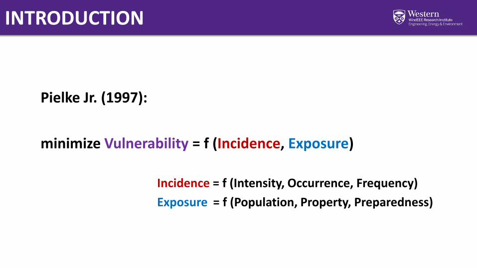
Pielke Jr. (1997):
minimize Vulnerability = f (Incidence, Exposure)
Incidence = f (Intensity, Occurrence, Frequency)
Exposure = f (Population, Property, Preparedness)
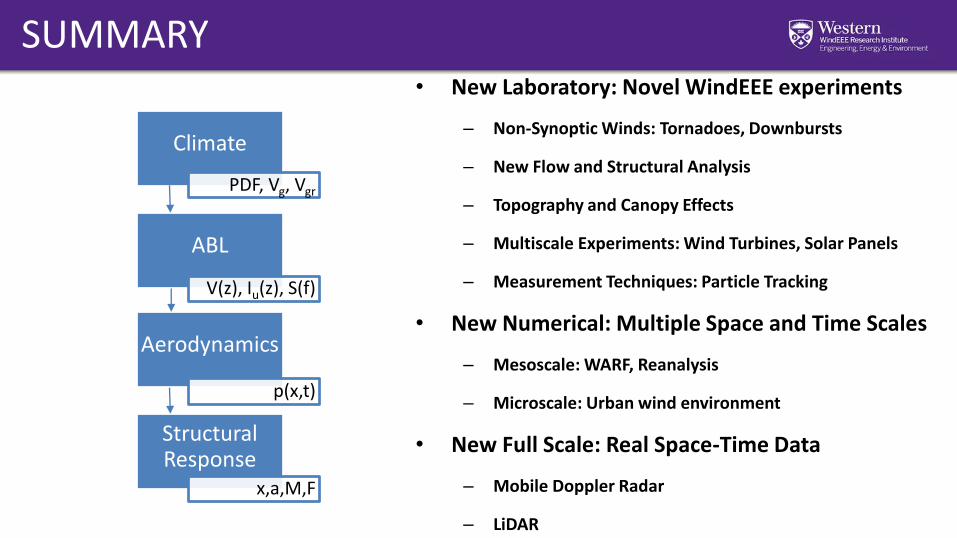
SUMMARY• New Laboratory: Novel WindEEE experiments
– Non-Synoptic Winds: Tornadoes, Downbursts
– New Flow and Structural Analysis
– Topography and Canopy Effects
– Multiscale Experiments: Wind Turbines, Solar Panels
– Measurement Techniques: Particle Tracking
• New Numerical: Multiple Space and Time Scales
– Mesoscale: WARF, Reanalysis
– Microscale: Urban wind environment
• New Full Scale: Real Space-Time Data
– Mobile Doppler Radar
– LiDAR
Climate
PDF, Vg, Vgr
ABL
V(z), Iu(z), S(f)
Aerodynamics
p(x,t)
Structural Response
x,a,M,F
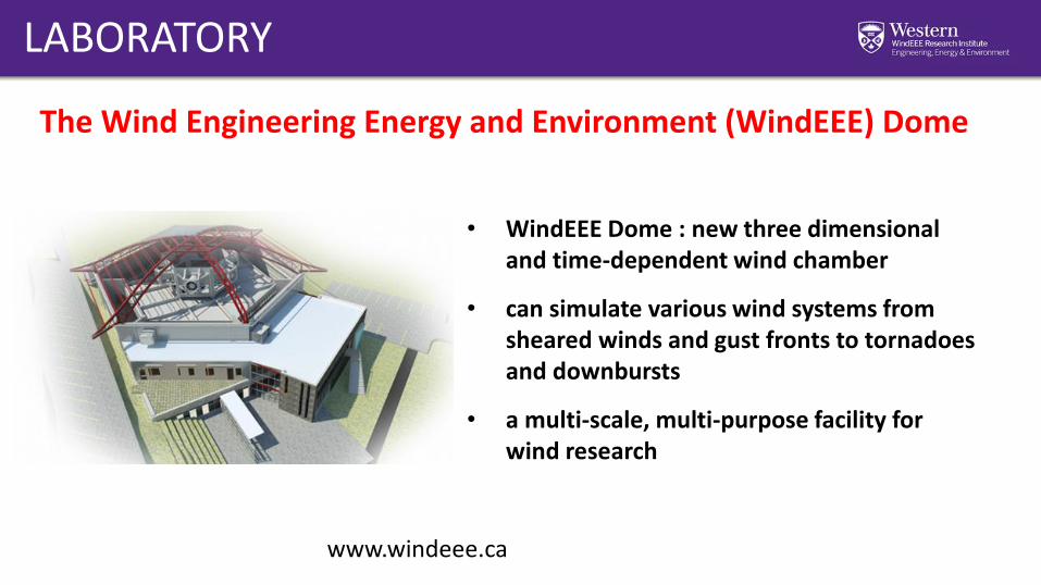
LABORATORY
• WindEEE Dome : new three dimensional and time-dependent wind chamber
• can simulate various wind systems from sheared winds and gust fronts to tornadoesand downbursts
• a multi-scale, multi-purpose facility for wind research
The Wind Engineering Energy and Environment (WindEEE) Dome
www.windeee.ca
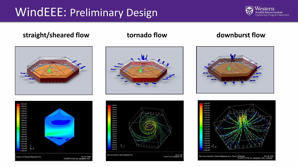
WindEEE: Preliminary Design
straight/sheared flow tornado flow downburst flow

WindEEE: Engineering Design
• 106 individually controlled fans
• 2 MW maximum power
• 5 m lift and turntable
• 1600 floor roughness elements
• 1000+ tons of steel
• 1850 m³ of concrete
• LEEDs Silver accreditation
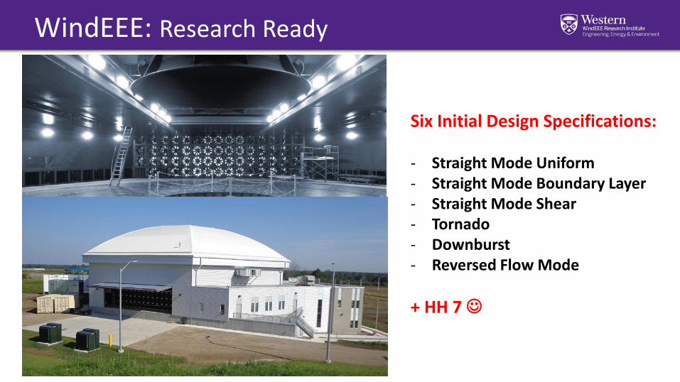
WindEEE: Research Ready
Six Initial Design Specifications:
- Straight Mode Uniform- Straight Mode Boundary Layer- Straight Mode Shear- Tornado- Downburst- Reversed Flow Mode
+ HH 7
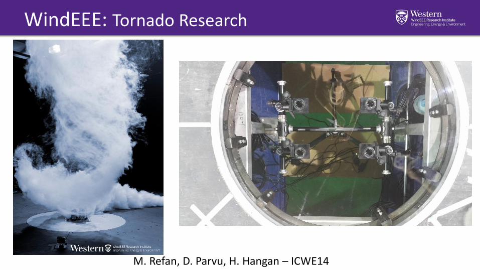
WindEEE: Tornado Research
M. Refan, D. Parvu, H. Hangan – ICWE14
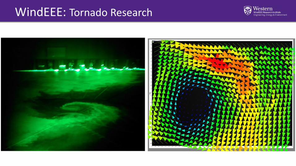
WindEEE: Tornado Research
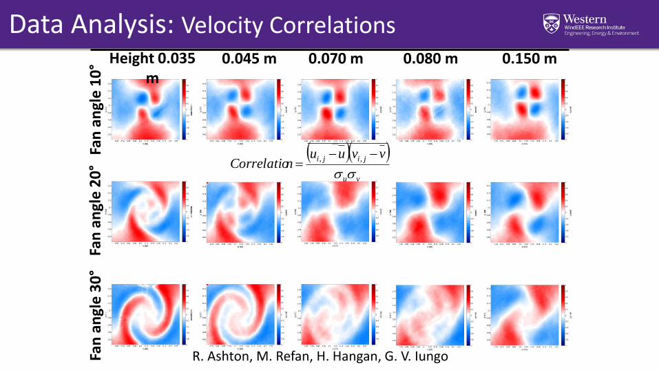
Data Analysis: Velocity Correlations
Fan
an
gle
10
°Fa
n a
ngl
e 2
0°
Fan
an
gle
30
°
Height 0.035 m
0.045 m 0.070 m 0.080 m 0.150 m
vu
jiji vvuunCorrelatio
,,
R. Ashton, M. Refan, H. Hangan, G. V. Iungo
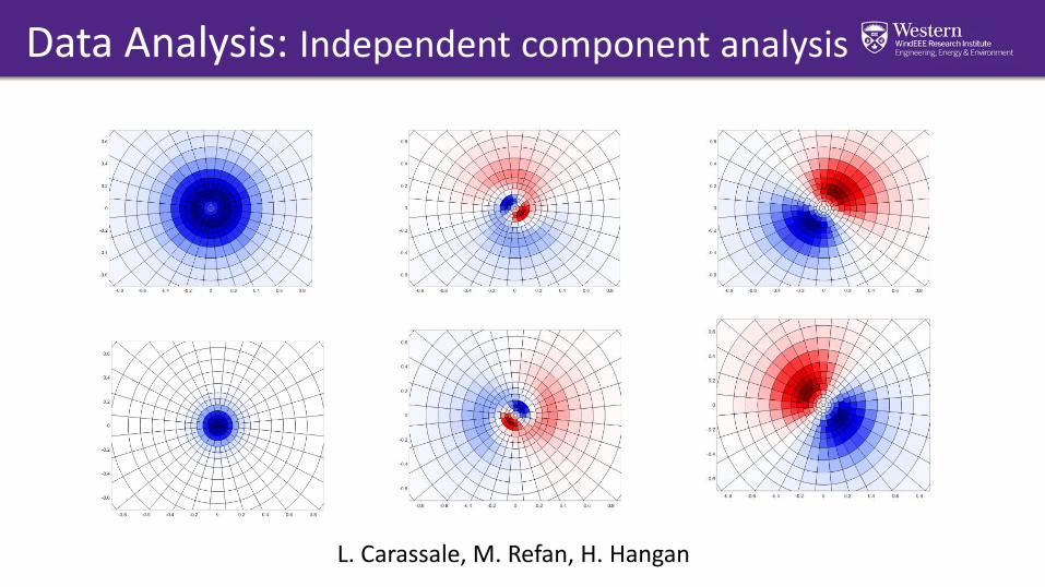
Data Analysis: Independent component analysis
L. Carassale, M. Refan, H. Hangan
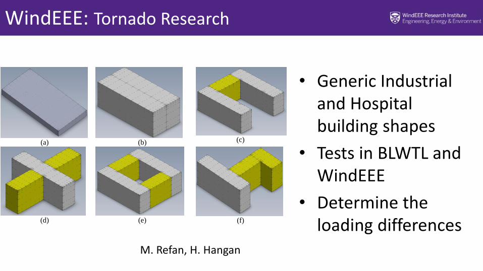
WindEEE: Tornado Research
(a)
(b)
(c)
(d)
(e)
(f)
• Generic Industrial and Hospital building shapes
• Tests in BLWTL and WindEEE
• Determine the loading differences
M. Refan, H. Hangan
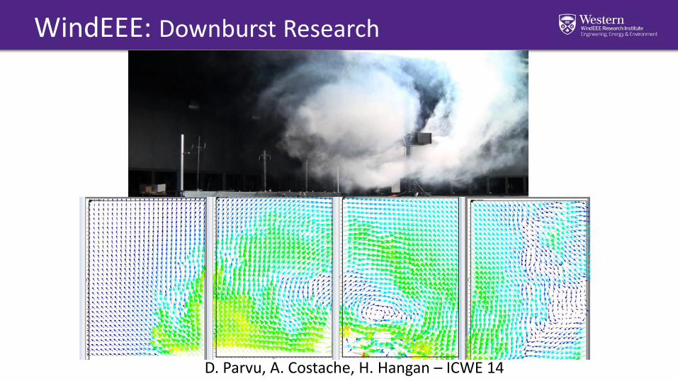
WindEEE: Downburst Research
D. Parvu, A. Costache, H. Hangan – ICWE 14
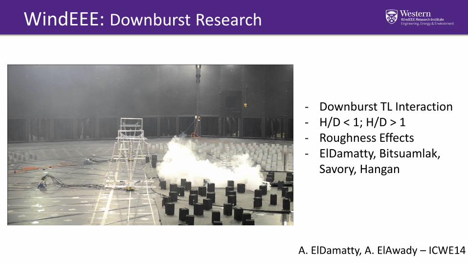
WindEEE: Downburst Research
- Downburst TL Interaction- H/D < 1; H/D > 1- Roughness Effects- ElDamatty, Bitsuamlak,
Savory, Hangan
A. ElDamatty, A. ElAwady – ICWE14
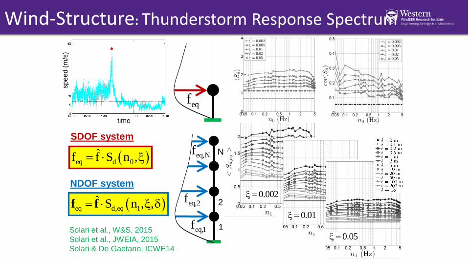
Wind-Structure: Thunderstorm Response Spectrum
eqf
eq d 0ˆf f S n ,
eq d,eq 1ˆ S n , , f f
SDOF system
NDOF system0.002
0.01
0.05 Solari et al., W&S, 2015
Solari et al., JWEIA, 2015
Solari & De Gaetano, ICWE14
time
sp
ee
d (
m/s
)
eq,Nf
eq,2f
eq,1f
N
2
1
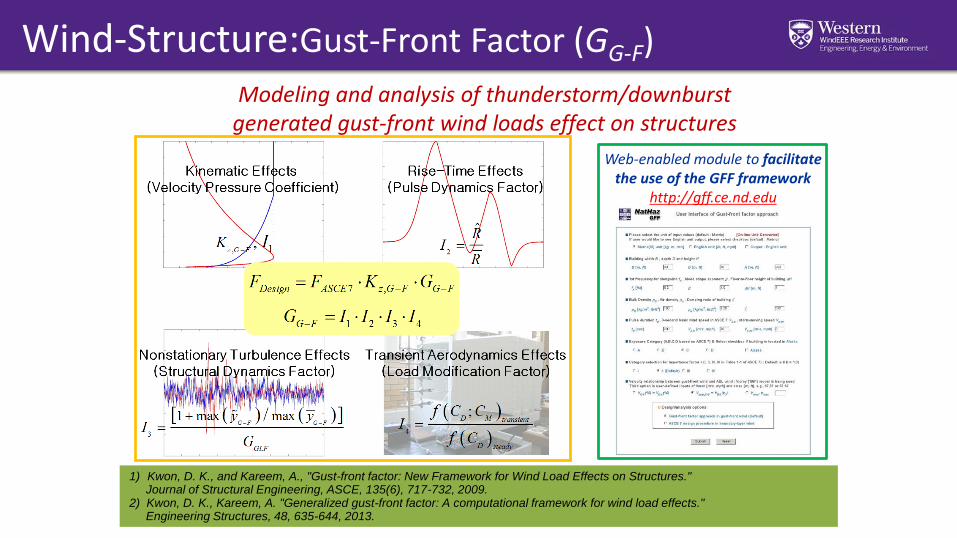
Wind-Structure:Gust-Front Factor (GG-F)
Modeling and analysis of thunderstorm/downburst generated gust-front wind loads effect on structures
Web-enabled module to facilitate the use of the GFF framework
http://gff.ce.nd.edu
1) Kwon, D. K., and Kareem, A., "Gust-front factor: New Framework for Wind Load Effects on Structures." Journal of Structural Engineering, ASCE, 135(6), 717-732, 2009.
2) Kwon, D. K., Kareem, A. "Generalized gust-front factor: A computational framework for wind load effects." Engineering Structures, 48, 635-644, 2013.
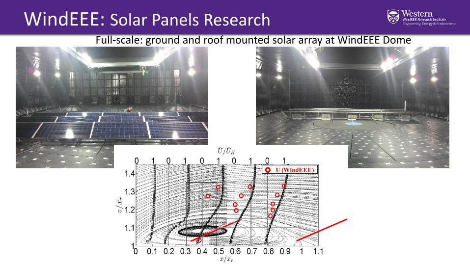
WindEEE: Solar Panels Research Full-scale: ground and roof mounted solar array at WindEEE Dome
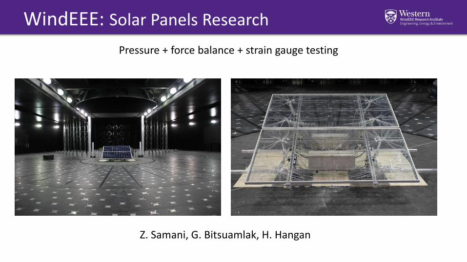
WindEEE: Solar Panels Research
Pressure + force balance + strain gauge testing
Z. Samani, G. Bitsuamlak, H. Hangan
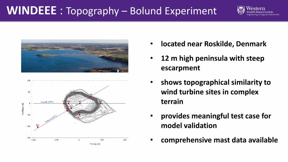
• located near Roskilde, Denmark
• 12 m high peninsula with steep escarpment
• shows topographical similarity to wind turbine sites in complex terrain
• provides meaningful test case for model validation
• comprehensive mast data available
WINDEEE : Topography – Bolund Experiment
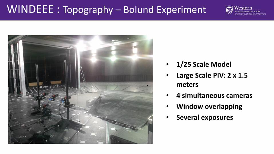
• 1/25 Scale Model
• Large Scale PIV: 2 x 1.5 meters
• 4 simultaneous cameras
• Window overlapping
• Several exposures
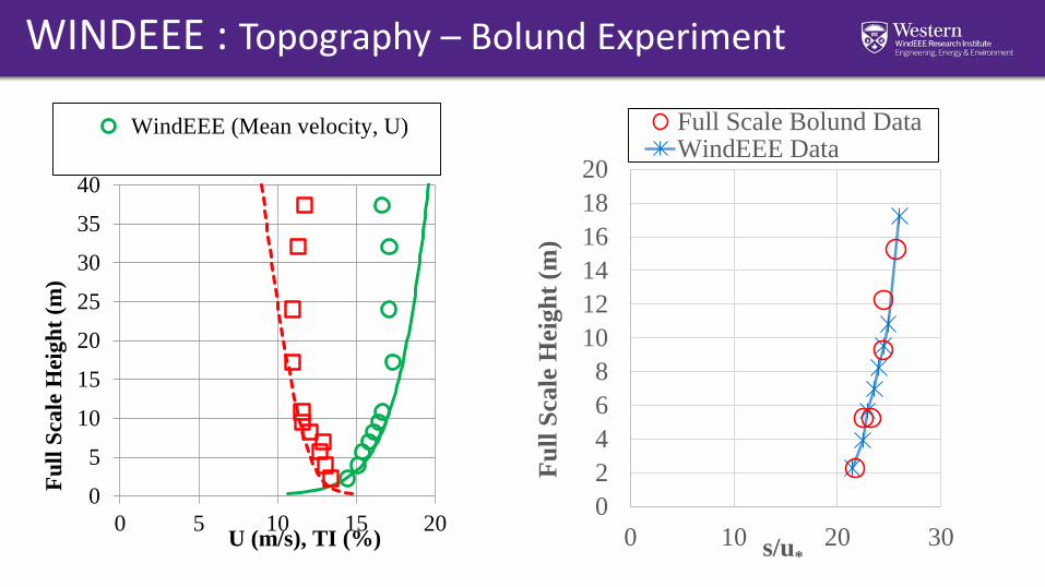
WINDEEE : Topography – Bolund Experiment
WINDEEE : Topography – Bolund Experiment
0
5
10
15
20
25
30
35
40
0 5 10 15 20
Fu
ll S
cale
Hei
gh
t (m
)
U (m/s), TI (%)
WindEEE (Mean velocity, U)
0
2
4
6
8
10
12
14
16
18
20
0 10 20 30F
ull
Sca
le H
eig
ht
(m)
s/u*
Full Scale Bolund DataWindEEE Data
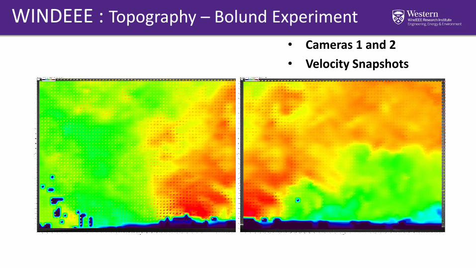
• Cameras 1 and 2
• Velocity Snapshots
WINDEEE : Topography – Bolund Experiment
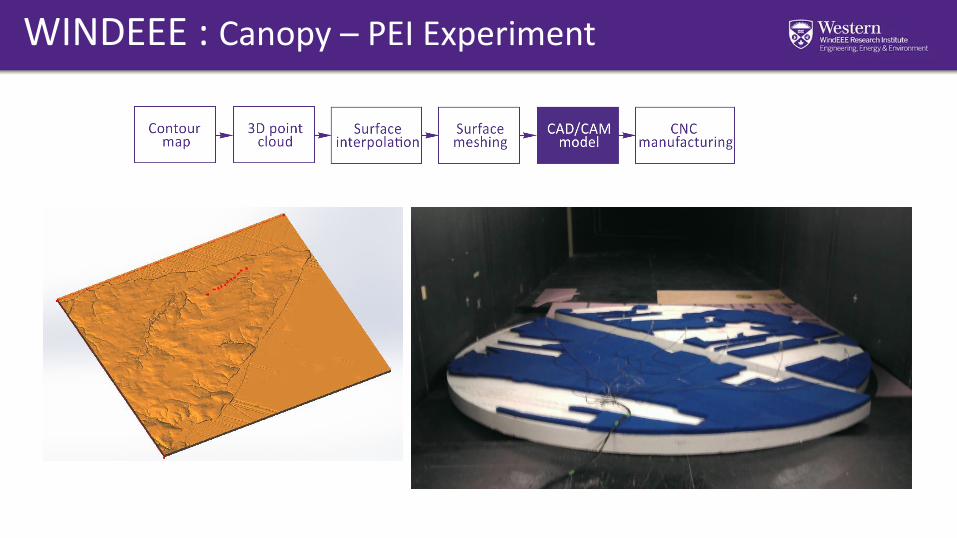
WINDEEE : Canopy – PEI Experiment
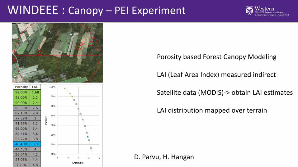
WINDEEE : Canopy – PEI Experiment
Porosity based Forest Canopy Modeling
LAI (Leaf Area Index) measured indirect
Satellite data (MODIS)-> obtain LAI estimates
LAI distribution mapped over terrain
D. Parvu, H. Hangan
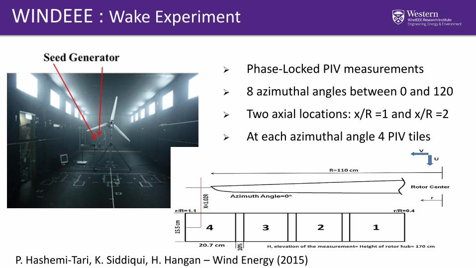
WINDEEE : Wake Experiment
Phase-Locked PIV measurements
8 azimuthal angles between 0 and 120
Two axial locations: x/R =1 and x/R =2
At each azimuthal angle 4 PIV tiles
P. Hashemi-Tari, K. Siddiqui, H. Hangan – Wind Energy (2015)
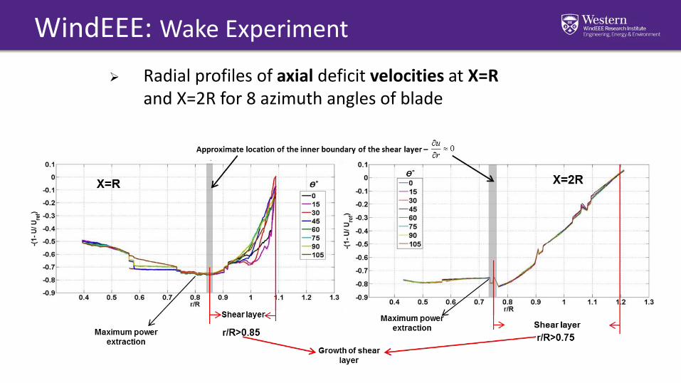
WindEEE: Wake Experiment
Radial profiles of axial deficit velocities at X=Rand X=2R for 8 azimuth angles of blade
WindEEE: Wake Experiment
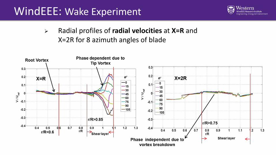
Radial profiles of radial velocities at X=R and X=2R for 8 azimuth angles of blade
WindEEE: Wake Experiment
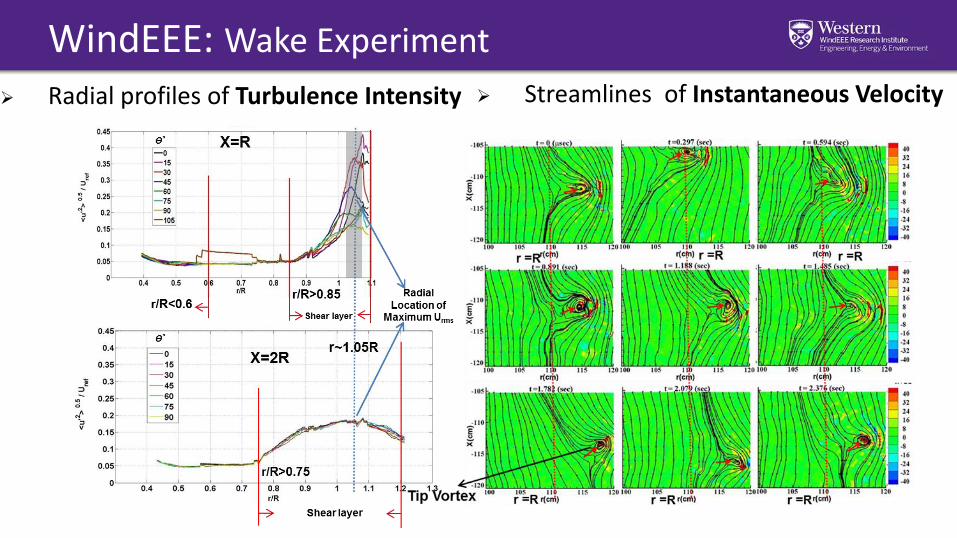
Radial profiles of Turbulence Intensity Streamlines of Instantaneous Velocity
WindEEE: Wake Experiment
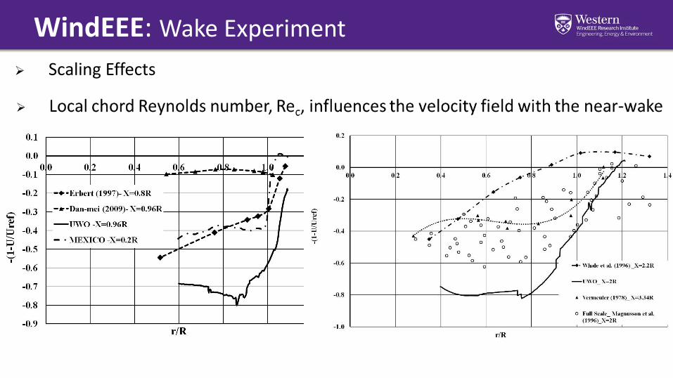
Scaling Effects
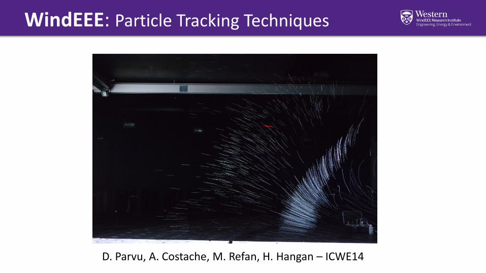
WindEEE: Particle Tracking Techniques
D. Parvu, A. Costache, M. Refan, H. Hangan – ICWE14
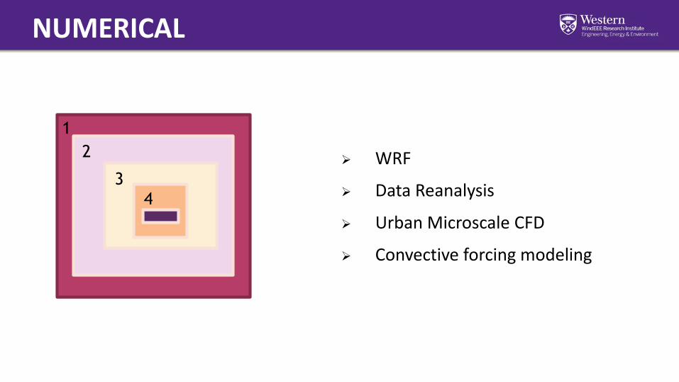
NUMERICAL
WRF
Data Reanalysis
Urban Microscale CFD
Convective forcing modeling
1
2
34
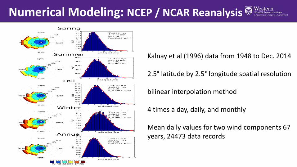
Numerical Modeling: NCEP / NCAR Reanalysis
Kalnay et al (1996) data from 1948 to Dec. 2014
2.5° latitude by 2.5° longitude spatial resolution
bilinear interpolation method
4 times a day, daily, and monthly
Mean daily values for two wind components 67 years, 24473 data records
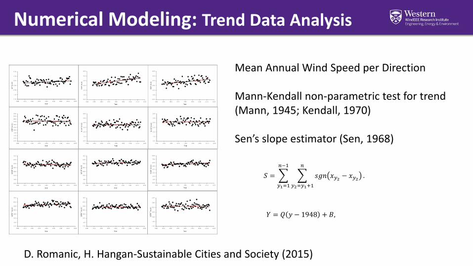
Numerical Modeling: Trend Data Analysis
Mean Annual Wind Speed per Direction
Mann-Kendall non-parametric test for trend (Mann, 1945; Kendall, 1970)
Sen’s slope estimator (Sen, 1968)
𝑆 =
𝑦1=1
𝑛−1
𝑦2=𝑦1+1
𝑛
𝑠𝑔𝑛 𝑥𝑦2 − 𝑥𝑦2 .
𝑌 = 𝑄 𝑦 − 1948 + 𝐵,
D. Romanic, H. Hangan-Sustainable Cities and Society (2015)
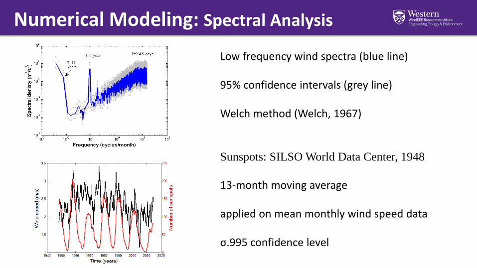
Numerical Modeling: Spectral Analysis
Low frequency wind spectra (blue line)
95% confidence intervals (grey line)
Welch method (Welch, 1967)
Sunspots: SILSO World Data Center, 1948
13-month moving average
applied on mean monthly wind speed data
σ.995 confidence level
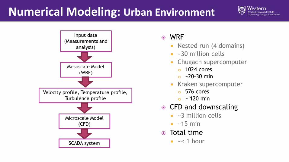
Numerical Modeling: Urban Environment
WRF Nested run (4 domains)
~30 million cells
Chugach supercomputer 1024 cores
~20-30 min
Kraken supercomputer 576 cores
~ 120 min
CFD and downscaling ~3 million cells
~15 min
Total time ~< 1 hour
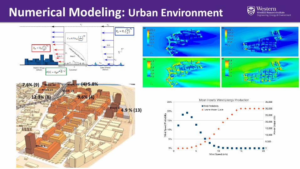
Numerical Modeling: Urban Environment
7.6% (9) (4) 5.8%
4.9 % (13)
12.3% (8) 9.6% (4)
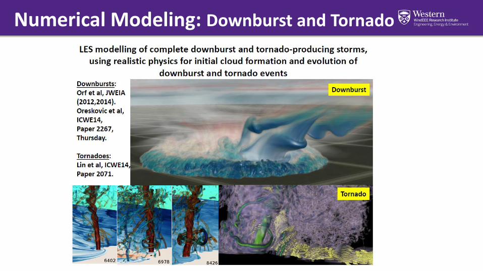
Numerical Modeling: Downburst and Tornado
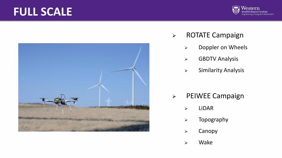
FULL SCALE
ROTATE Campaign
Doppler on Wheels
GBDTV Analysis
Similarity Analysis
PEIWEE Campaign
LiDAR
Topography
Canopy
Wake
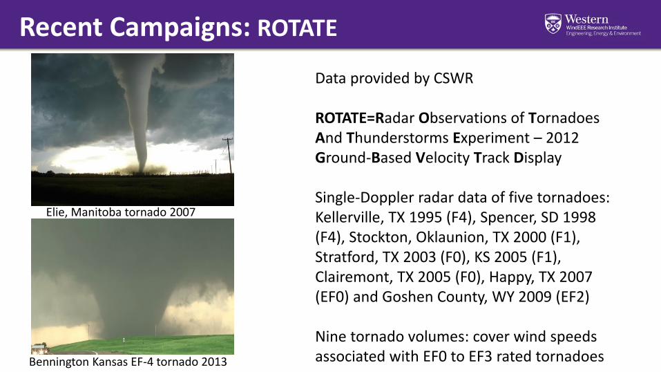
Recent Campaigns: ROTATE
Data provided by CSWR
ROTATE=Radar Observations of Tornadoes And Thunderstorms Experiment – 2012Ground-Based Velocity Track Display
Single-Doppler radar data of five tornadoes: Kellerville, TX 1995 (F4), Spencer, SD 1998 (F4), Stockton, Oklaunion, TX 2000 (F1), Stratford, TX 2003 (F0), KS 2005 (F1), Clairemont, TX 2005 (F0), Happy, TX 2007 (EF0) and Goshen County, WY 2009 (EF2)
Nine tornado volumes: cover wind speeds associated with EF0 to EF3 rated tornadoes
Elie, Manitoba tornado 2007
Bennington Kansas EF-4 tornado 2013
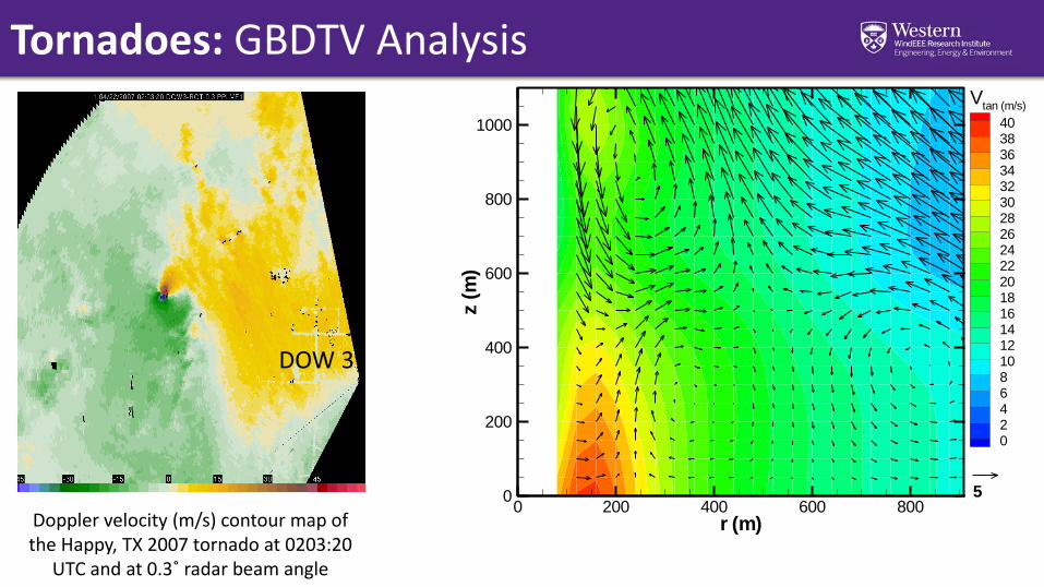
Tornadoes: GBDTV Analysis
DOW 3
Doppler velocity (m/s) contour map of the Happy, TX 2007 tornado at 0203:20
UTC and at 0.3˚ radar beam angle
r (m)
z(m
)
0 200 400 600 8000
200
400
600
800
1000
Vtan (m/s)
4038363432302826242220181614121086420
5
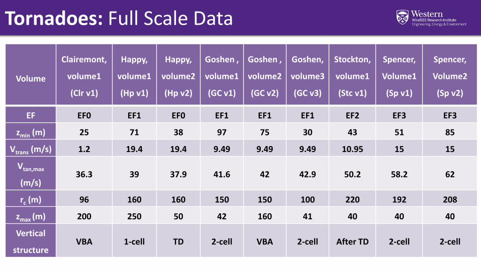
Tornadoes: Full Scale Data
Volume
Clairemont,
volume1
(Clr v1)
Happy,
volume1
(Hp v1)
Happy,
volume2
(Hp v2)
Goshen ,
volume1
(GC v1)
Goshen ,
volume2
(GC v2)
Goshen,
volume3
(GC v3)
Stockton,
volume1
(Stc v1)
Spencer,
Volume1
(Sp v1)
Spencer,
Volume2
(Sp v2)
EF EF0 EF1 EF0 EF1 EF1 EF1 EF2 EF3 EF3
zmin (m) 25 71 38 97 75 30 43 51 85
Vtrans (m/s) 1.2 19.4 19.4 9.49 9.49 9.49 10.95 15 15
Vtan,max
(m/s)36.3 39 37.9 41.6 42 42.9 50.2 58.2 62
rc (m) 96 160 160 150 150 100 220 192 208
zmax (m) 200 250 50 42 160 41 40 40 40
Vertical
structureVBA 1-cell TD 2-cell VBA 2-cell After TD 2-cell 2-cell
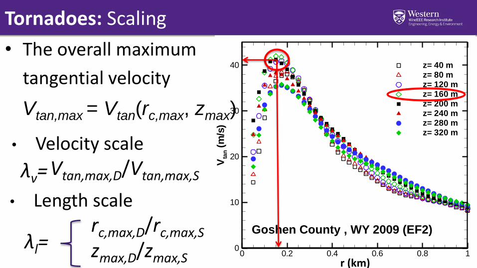
Tornadoes: Scaling
R (km)
Vta
n(m
/s)
0 0.2 0.4 0.6 0.8 10
10
20
30
40 z= 40 mz= 80 mz= 120 mz= 160 mz= 200 mz= 240 mz= 280 mz= 320 m
Goshen County , WY 2009 (EF2)
• The overall maximum
tangential velocity
Vtan,max = Vtan(rc,max, zmax)
• Length scale
rc,max,D/rc,max,S
zmax,D/zmax,Sλl=
r (km)
λv=
• Velocity scale
Vtan,max,D/Vtan,max,S
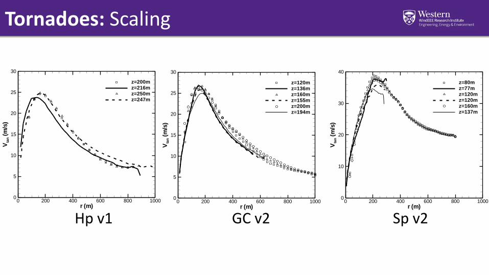
Tornadoes: Scaling
Hp v1 GC v2 Sp v2r (m)
Vta
n(m
/s)
0 200 400 600 800 10000
5
10
15
20
25
30
z=120mz=136mz=160mz=155mz=200mz=194m
r (m)
Vta
n(m
/s)
0 200 400 600 800 10000
5
10
15
20
25
30
z=200mz=216mz=250mz=247m
r (m)
Vta
n(m
/s)
0 200 400 600 800 10000
10
20
30
40
z=80mz=77mz=120mz=120mz=160mz=137m
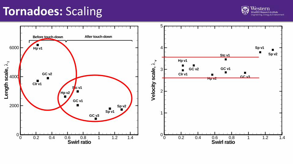
Tornadoes: Scaling
Swirl ratio
Len
gth
scale
,
l
0 0.2 0.4 0.6 0.8 1 1.2 1.40
2000
4000
6000
Before touch-down After touch-down
Clr v1
Hp v1
Hp v2
Stc v1
GC v1
GC v2
GC v3Sp v1
Sp v2
Swirl ratio
Velo
city
scale
,
v
0 0.2 0.4 0.6 0.8 1 1.2 1.40
1
2
3
4
5
Hp v1
Clr v1
Hp v2
GC v1GC v2
GC v3
Sp v1
Sp v2Stc v1
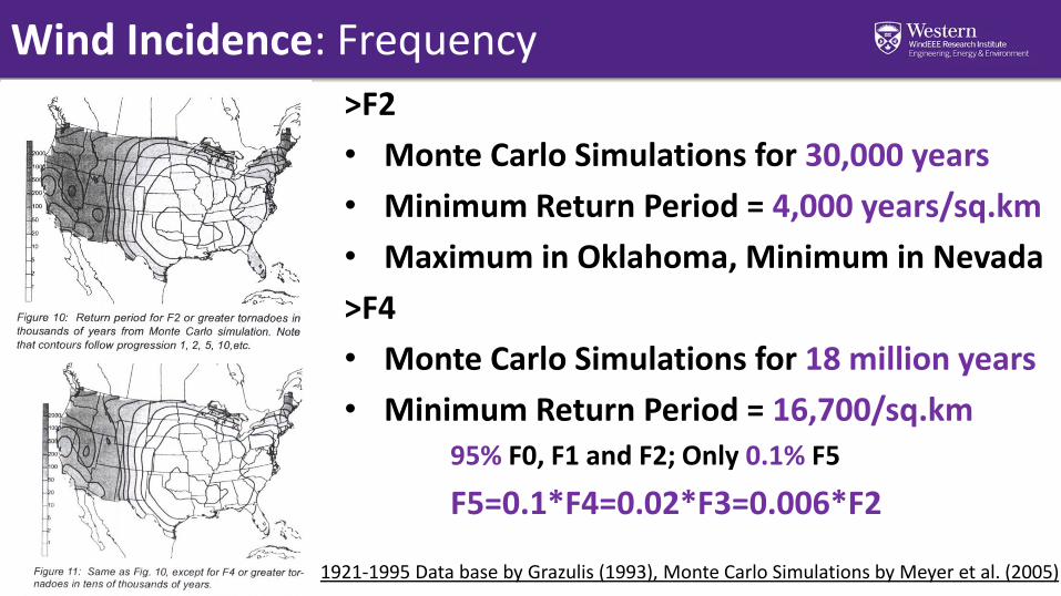
>F2
• Monte Carlo Simulations for 30,000 years
• Minimum Return Period = 4,000 years/sq.km
• Maximum in Oklahoma, Minimum in Nevada
>F4
• Monte Carlo Simulations for 18 million years
• Minimum Return Period = 16,700/sq.km95% F0, F1 and F2; Only 0.1% F5
F5=0.1*F4=0.02*F3=0.006*F2
Wind Incidence: Frequency
1921-1995 Data base by Grazulis (1993), Monte Carlo Simulations by Meyer et al. (2005)
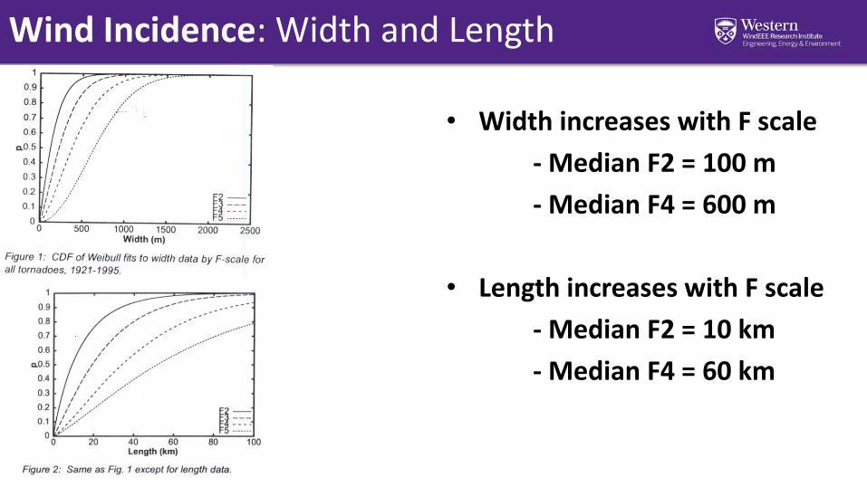
• Width increases with F scale
- Median F2 = 100 m
- Median F4 = 600 m
• Length increases with F scale
- Median F2 = 10 km
- Median F4 = 60 km
Wind Incidence: Width and Length
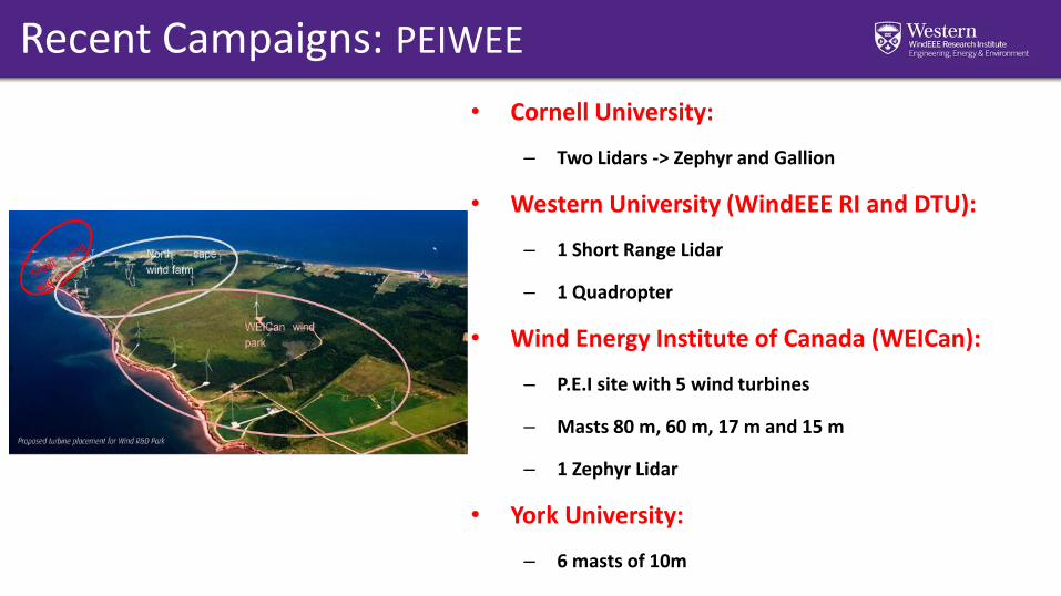
Recent Campaigns: PEIWEE
• Cornell University:
– Two Lidars -> Zephyr and Gallion
• Western University (WindEEE RI and DTU):
– 1 Short Range Lidar
– 1 Quadropter
• Wind Energy Institute of Canada (WEICan):
– P.E.I site with 5 wind turbines
– Masts 80 m, 60 m, 17 m and 15 m
– 1 Zephyr Lidar
• York University:
– 6 masts of 10m
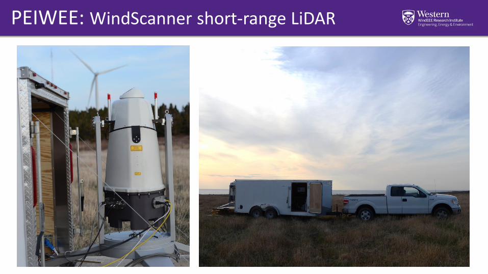
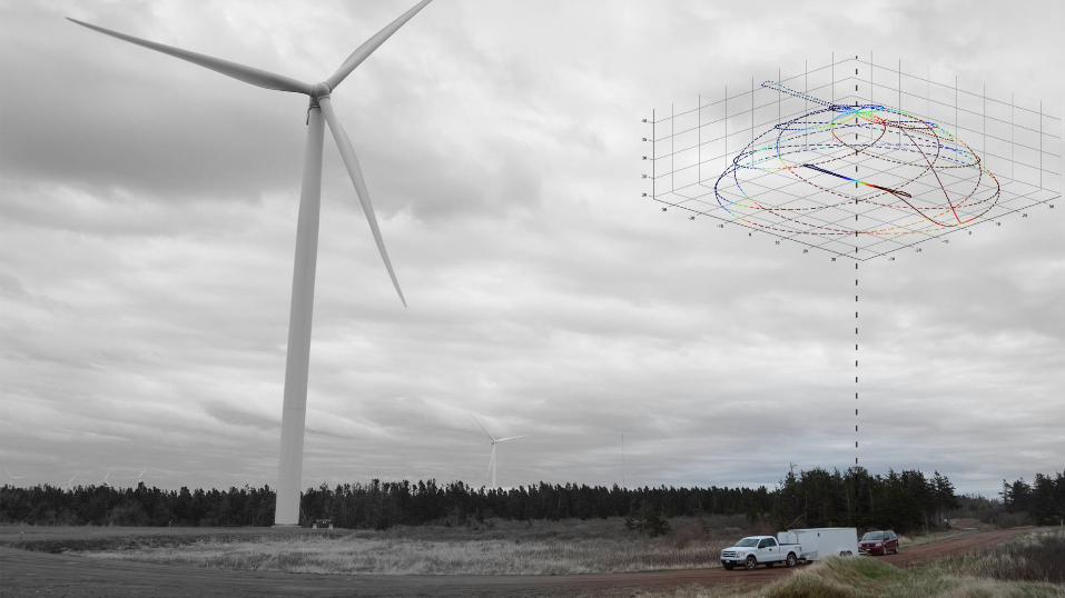
PEIWEE: WindScanner short-range LiDAR
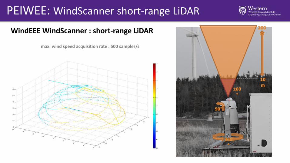
PEIWEE: WindScanner short-range LiDAR
WindEEE WindScanner : short-range LiDAR
max. wind speed acquisition rate : 500 samples/s
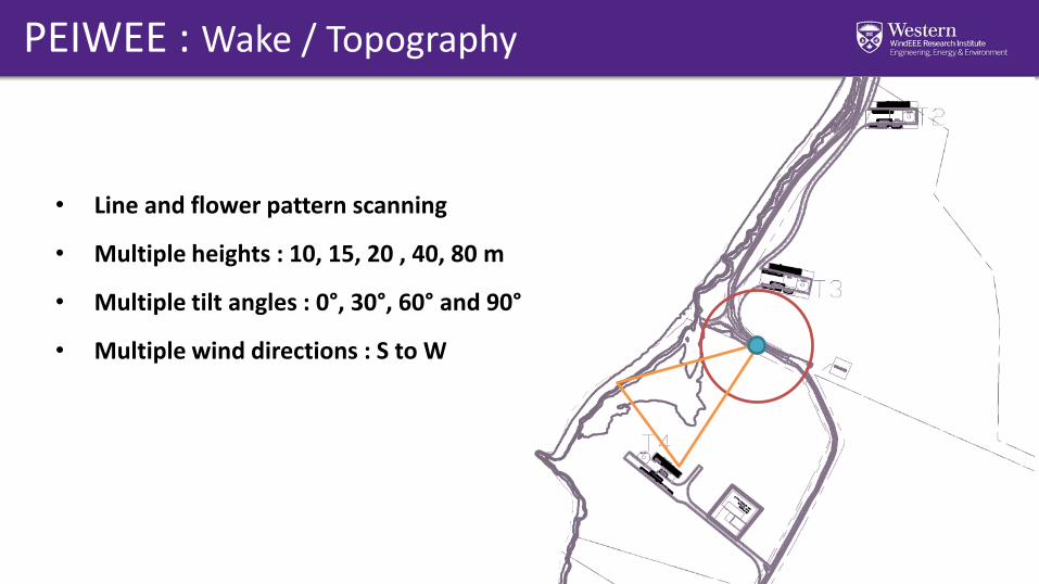
PEIWEE : Wake / Topography
• Line and flower pattern scanning
• Multiple heights : 10, 15, 20 , 40, 80 m
• Multiple tilt angles : 0°, 30°, 60° and 90°
• Multiple wind directions : S to W
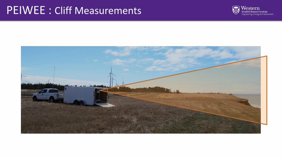
PEIWEE : Cliff Measurements
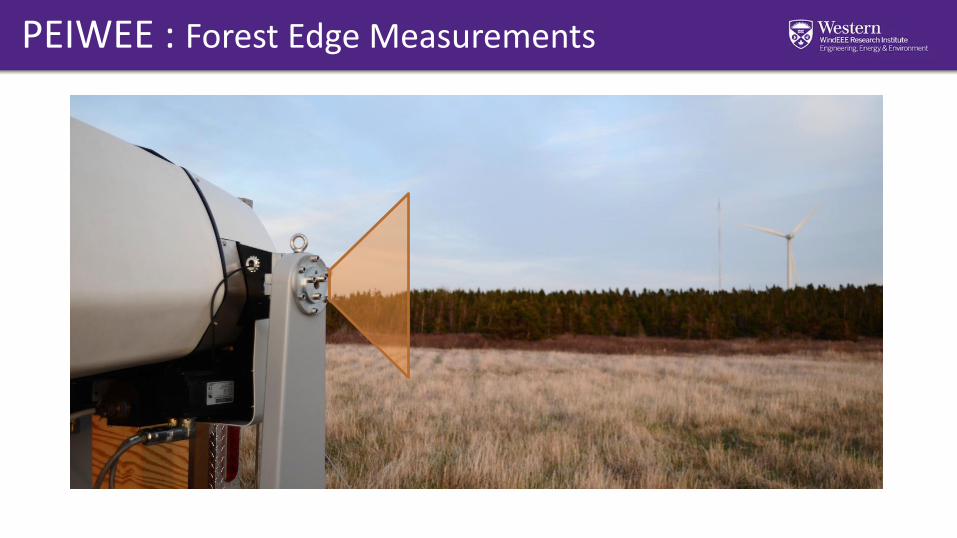
PEIWEE : Forest Edge Measurements
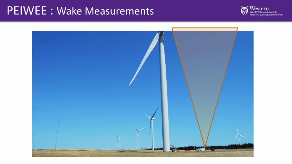
PEIWEE : Wake Measurements
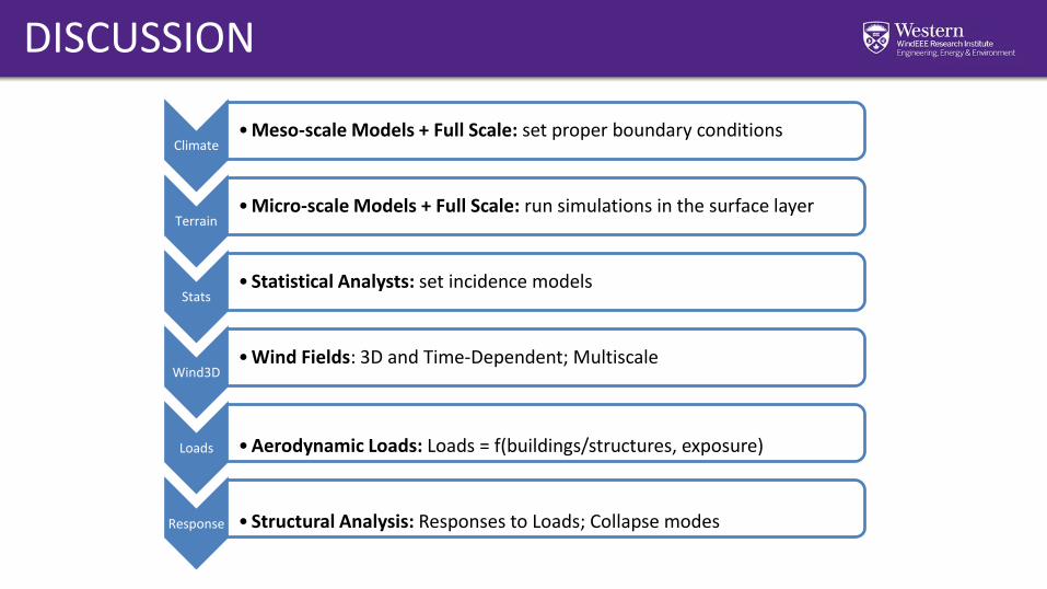
DISCUSSION
Climate• Meso-scale Models + Full Scale: set proper boundary conditions
Terrain• Micro-scale Models + Full Scale: run simulations in the surface layer
Stats• Statistical Analysts: set incidence models
Wind3D• Wind Fields: 3D and Time-Dependent; Multiscale
Loads • Aerodynamic Loads: Loads = f(buildings/structures, exposure)
Response • Structural Analysis: Responses to Loads; Collapse modes
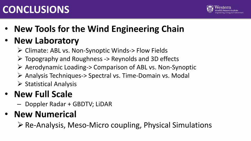
CONCLUSIONS
• New Tools for the Wind Engineering Chain • New Laboratory
Climate: ABL vs. Non-Synoptic Winds-> Flow Fields Topography and Roughness -> Reynolds and 3D effects Aerodynamic Loading-> Comparison of ABL vs. Non-Synoptic Analysis Techniques-> Spectral vs. Time-Domain vs. Modal Statistical Analysis
• New Full Scale– Doppler Radar + GBDTV; LiDAR
• New NumericalRe-Analysis, Meso-Micro coupling, Physical Simulations
REFERENCES
- Pielke Jr., R.A., Refraining the U.S. hurricane problem, Society &Natural Resources: 1997.- Grazulis, T.P., Significant Tornadoes, 1680-1991. Environmental Films, St. Johnsbury, VT, 1326, 1993.- Meyer, C. L, Brooks, H. E. and Kay, M. P., A hazard model for tornado occurrence in the United States, 16th Conference on Probability and Statistics in the Atmospheric Sciences, 2002.- Xu, Z. and Hangan, H., Scale, boundary and inlet condition effects on impinging jets with application to downburst simulations, J. of Wind Eng. and Ind. Aerodynamics, 96,2008.- Hangan, H. and Kim, J.D.*, Numerical characterization of impinging jets with application to downbursts. J. of Wind Eng. and Ind. Aerodynamics, 95, Issue 4,2007.- Refan, M.*, Hangan, H., Wurman, J., “Reproducing Tornadoes in Laboratory Using Proper Scaling”, J. Wind Eng. And Ind. Aerodynamics, 2014-Hashemi-Tari, P*.,Hangan, H., Siddiqui, K., “Flow characterization in the Near-wake region of a Horizontal Axis Wind Turbine”, Wind Energy (2015) - Romanic, D.*, Rasouli, A.*, Hangan, H., “Wind resource assessment in complex urban environment”, Wind Engineering, Vol. 39, Nr. 2, January 2015- Romanic, D., Hangan, H., “Wind Climatology of Toronto based on NCEP/NCAR reanalysis 1 data set and its potential relation to solar activity, Sustainable Cities and Society (2015)
-
Thank You !
www.windeee.ca