Embed Size (px)
Citation preview

Unbounded linear operators
Jan Derezinski
Department of Mathematical Methods in Physics
Faculty of Physics
University of Warsaw
Hoza 74, 00-682, Warszawa, Poland
Lecture notes, version of June 2013


Contents
1 Unbounded operators on Banach spaces 13
1.1 Relations . . . . . . . . . . . . . . . . . . . . . . . . . . . . . . . . . . . . . 13
1.2 Linear partial operators . . . . . . . . . . . . . . . . . . . . . . . . . . . . . 17
1.3 Closed operators . . . . . . . . . . . . . . . . . . . . . . . . . . . . . . . . . 18
1.4 Bounded operators . . . . . . . . . . . . . . . . . . . . . . . . . . . . . . . . 20
1.5 Closable operators . . . . . . . . . . . . . . . . . . . . . . . . . . . . . . . . 21
1.6 Essential domains . . . . . . . . . . . . . . . . . . . . . . . . . . . . . . . . 23
1.7 Perturbations of closed operators . . . . . . . . . . . . . . . . . . . . . . . . 24
3

1.8 Invertible unbounded operators . . . . . . . . . . . . . . . . . . . . . . . . . 28
1.9 Spectrum of unbounded operators . . . . . . . . . . . . . . . . . . . . . . . . 32
1.10 Functional calculus . . . . . . . . . . . . . . . . . . . . . . . . . . . . . . . . 36
1.11 Spectral idempotents . . . . . . . . . . . . . . . . . . . . . . . . . . . . . . 41
1.12 Examples of unbounded operators . . . . . . . . . . . . . . . . . . . . . . . . 43
1.13 Pseudoresolvents . . . . . . . . . . . . . . . . . . . . . . . . . . . . . . . . . 45
2 One-parameter semigroups on Banach spaces 47
2.1 (M,β)-type semigroups . . . . . . . . . . . . . . . . . . . . . . . . . . . . . 47
2.2 Generator of a semigroup . . . . . . . . . . . . . . . . . . . . . . . . . . . . 49
2.3 One-parameter groups . . . . . . . . . . . . . . . . . . . . . . . . . . . . . . 54
2.4 Norm continuous semigroups . . . . . . . . . . . . . . . . . . . . . . . . . . 55
2.5 Essential domains of generators . . . . . . . . . . . . . . . . . . . . . . . . . 56
2.6 Operators of (M,β)-type . . . . . . . . . . . . . . . . . . . . . . . . . . . . 58
2.7 The Hille-Philips-Yosida theorem . . . . . . . . . . . . . . . . . . . . . . . . 60
2.8 Semigroups of contractions and their generators . . . . . . . . . . . . . . . . 65

3 Unbounded operators on Hilbert spaces 67
3.1 Graph scalar product . . . . . . . . . . . . . . . . . . . . . . . . . . . . . . . 67
3.2 The adjoint of an operator . . . . . . . . . . . . . . . . . . . . . . . . . . . . 68
3.3 Inverse of the adjoint operator . . . . . . . . . . . . . . . . . . . . . . . . . . 72
3.4 Numerical range and maximal operators . . . . . . . . . . . . . . . . . . . . . 74
3.5 Dissipative operators . . . . . . . . . . . . . . . . . . . . . . . . . . . . . . . 78
3.6 Hermitian operators . . . . . . . . . . . . . . . . . . . . . . . . . . . . . . . 80
3.7 Self-adjoint operators . . . . . . . . . . . . . . . . . . . . . . . . . . . . . . 82
3.8 Spectral theorem . . . . . . . . . . . . . . . . . . . . . . . . . . . . . . . . . 85
3.9 Essentially self-adjoint operators . . . . . . . . . . . . . . . . . . . . . . . . . 89
3.10 Rigged Hilbert space . . . . . . . . . . . . . . . . . . . . . . . . . . . . . . . 90
3.11 Polar decomposition . . . . . . . . . . . . . . . . . . . . . . . . . . . . . . . 94
3.12 Scale of Hilbert spaces I . . . . . . . . . . . . . . . . . . . . . . . . . . . . . 98
3.13 Scale of Hilbert spaces II . . . . . . . . . . . . . . . . . . . . . . . . . . . . . 100
3.14 Complex interpolation . . . . . . . . . . . . . . . . . . . . . . . . . . . . . . 101

3.15 Relative operator boundedness . . . . . . . . . . . . . . . . . . . . . . . . . . 104
3.16 Relative form boundedness . . . . . . . . . . . . . . . . . . . . . . . . . . . . 105
3.17 Self-adjointness of Schrodinger operators . . . . . . . . . . . . . . . . . . . . 109
4 Positive forms 115
4.1 Quadratic forms . . . . . . . . . . . . . . . . . . . . . . . . . . . . . . . . . 115
4.2 Sesquilinear quasiforms . . . . . . . . . . . . . . . . . . . . . . . . . . . . . 117
4.3 Closed positive forms . . . . . . . . . . . . . . . . . . . . . . . . . . . . . . 119
4.4 Closable positive forms . . . . . . . . . . . . . . . . . . . . . . . . . . . . . . 121
4.5 Operators associated with positive forms . . . . . . . . . . . . . . . . . . . . 123
4.6 Perturbations of positive forms . . . . . . . . . . . . . . . . . . . . . . . . . 124
4.7 Friedrichs extensions . . . . . . . . . . . . . . . . . . . . . . . . . . . . . . . 126
5 Non-maximal operators 129
5.1 Defect indices . . . . . . . . . . . . . . . . . . . . . . . . . . . . . . . . . . 130
5.2 Extensions of hermitian operators . . . . . . . . . . . . . . . . . . . . . . . . 132

5.3 Extension of positive operators . . . . . . . . . . . . . . . . . . . . . . . . . 137
6 Aronszajn-Donoghue Hamiltonians and their renormalization 141
6.1 Construction . . . . . . . . . . . . . . . . . . . . . . . . . . . . . . . . . . . 142
6.2 Cut-off method . . . . . . . . . . . . . . . . . . . . . . . . . . . . . . . . . . 147
6.3 Extensions of hermitian operators . . . . . . . . . . . . . . . . . . . . . . . . 149
6.4 Positive H0 . . . . . . . . . . . . . . . . . . . . . . . . . . . . . . . . . . . . 150
7 Friedrichs Hamiltonians and their renormalization 155
7.1 Construction . . . . . . . . . . . . . . . . . . . . . . . . . . . . . . . . . . . 156
7.2 The cut-off method . . . . . . . . . . . . . . . . . . . . . . . . . . . . . . . 160
7.3 Eigenvectors and resonances . . . . . . . . . . . . . . . . . . . . . . . . . . . 162
7.4 Dissipative semigroup from a Friedrichs Hamiltonian . . . . . . . . . . . . . . 164
8 Momentum in one dimension 167
8.1 Distributions on R . . . . . . . . . . . . . . . . . . . . . . . . . . . . . . . . 167
8.2 Momentum on the line . . . . . . . . . . . . . . . . . . . . . . . . . . . . . . 168

8.3 Momentum on the half-line . . . . . . . . . . . . . . . . . . . . . . . . . . . 174
8.4 Momentum on an interval I . . . . . . . . . . . . . . . . . . . . . . . . . . . 176
8.5 Momentum on an interval II . . . . . . . . . . . . . . . . . . . . . . . . . . . 178
8.6 Momentum on an interval III . . . . . . . . . . . . . . . . . . . . . . . . . . 179
9 Laplacian 181
9.1 Sobolev spaces in one dimension . . . . . . . . . . . . . . . . . . . . . . . . 181
9.2 Laplacian on the line . . . . . . . . . . . . . . . . . . . . . . . . . . . . . . . 182
9.3 Laplacian on the halfline I . . . . . . . . . . . . . . . . . . . . . . . . . . . . 185
9.4 Laplacian on the halfline II . . . . . . . . . . . . . . . . . . . . . . . . . . . . 187
9.5 Neumann Laplacian on a halfline with the delta potential . . . . . . . . . . . . 190
9.6 Dirichlet Laplacian on a halfline with the δ′ potential . . . . . . . . . . . . . . 192
9.7 Laplacian on L2(Rd) with the delta potential . . . . . . . . . . . . . . . . . . 194
9.8 Approximating delta potentials by separable potentials . . . . . . . . . . . . . 202
10 Orthogonal polynomials 205
10.1 Orthogonal polynomials . . . . . . . . . . . . . . . . . . . . . . . . . . . . . 207
10.2 Reminder about hermitian operators . . . . . . . . . . . . . . . . . . . . . . . 209
10.3 2nd order differential operators . . . . . . . . . . . . . . . . . . . . . . . . . 211
10.4 Hypergeometric type operators . . . . . . . . . . . . . . . . . . . . . . . . . 214
10.5 Generalized Rodrigues formula . . . . . . . . . . . . . . . . . . . . . . . . . . 216
10.6 Classical orthogonal polynomials as eigenfunctions of a Sturm-Liouville operator 221
10.7 Classical orthogonal polynomials for deg σ = 0 . . . . . . . . . . . . . . . . . 223
10.8 Classical orthogonal polynomials for deg σ = 1 . . . . . . . . . . . . . . . . . 225
10.9 Classical orthogonal polynomials for deg σ = 2,
σ has a double root . . . . . . . . . . . . . . . . . . . . . . . . . . . . . . . 226
10.10Classical orthogonal polynomials for deg σ = 2,
σ has two roots . . . . . . . . . . . . . . . . . . . . . . . . . . . . . . . . . 227
11 Homogeneous Schrodinger operators 229
11.1 Modified Bessel equation . . . . . . . . . . . . . . . . . . . . . . . . . . . . 229
11.2 Standard Bessel equation . . . . . . . . . . . . . . . . . . . . . . . . . . . . 233

11.3 Homogeneous Schrodinger operators . . . . . . . . . . . . . . . . . . . . . . 236
11.4 Factorization . . . . . . . . . . . . . . . . . . . . . . . . . . . . . . . . . . . 242
11.5 Hm as a holomorphic family of closed operators . . . . . . . . . . . . . . . . 246

Unbounded operators is a relatively technical and complicated subject. To my knowledge,
in most mathematics departments of the world it does not belong to the standard curricu-
lum, except maybe for some rudimentary elements. Most courses of functional analysis limit
themselves to bounded operators, which are much cleaner and easier to discuss.
Of course, in physics departments unbounded operators do not belong to the standard
curriculum either. However, implicitly, they appear very often in physics courses. In fact, many
operators relevant for applications are unbounded.
These lecture notes grew out of a course “Mathematics of quantum theory” given at Faculty
of Physics, University of Warsaw. The aim of the course was not only to give a general theory
of unbounded operators, but also to illustrate it with many interesting examples.


Chapter 1
Unbounded operators on Banach spaces
1.1 Relations
One of the problems with unbounded operators is that they are not true operators. In order
to avoid confusion, it is helpful to begin with a reexamination the concepts of functions and
relations.
Let X, Y be sets. R is called a relation iff R ⊂ Y × X. We will also write R : X → Y .
13

(Note the inversion of the direction). An example of a relation is the identity
1lX := (x, x) : x ∈ X ⊂ X ×X.
Introduce the projections
Y ×X 3 (y, x) 7→ πY (y, x) := y ∈ Y,
Y ×X 3 (y, x) 7→ πX(y, x) := x ∈ X,
and the flip
Y ×X 3 (y, x) 7→ τ(y, x) := (x, y) ∈ X × Y.
The domain of R is defined as DomR := πXR, its range is RanR = πYR, the inverse of R is
defined as R−1 := τR ⊂ X × Y . If S ⊂ Z × Y , then the superposition of S and R is defined
as
S R := (z, x) ∈ Z ×X : ∃y∈Y (z, y) ∈ S, (y, x) ∈ R.

If X0 ⊂ X, then the restriction of R to X0 is defined as
R∣∣∣X0
:= R ∩ Y×X0.
If, moreover, Y0 ⊂ Y , then
R∣∣∣X0→Y0
:= R ∩ Y0×X0.
We say that a relation R is injective, if πX(R∩y×X) is one-element for any y ∈ RanR.
We say that R is surjective if RanR = Y .
We say that a relation R is coinjective, if πY (R∩Y×x) is one-element for any x ∈ DomR.
We say that R is cosurjective if DomR = X.
Proposition 1.1.1 a) If R, S are coinjective, then so is S R.
b) If R, S are cosurjective, then so does S R.
In a basic course of set theory we learn that a coinjective cosurjective relation is called a
function. One also introduce many synonims of this word, such as a transformation, operator,
map, etc.

To speak about ubounded operators we will need a more general concept. A coinjective
relation will be called a partial transformation (or a partial operator, etc).
We also introduce the graph of R:
GrR := (x, y) ∈ X × Y : (y, x) ∈ R.
Strictly speaking GrR = τR. The difference between GrR and R lies only in their syntactic
role.
Note that the order Y ×X is convenient for the definition of superposition. However, it is
not the usual choice. In the sequel, instead of writing (y, x) ∈ R, we will write y = R(x) or
(x, y) ∈ GrR.
A superposition of partial transformations is a partial transformation. The inverse of a partial
transformation is a partial transformation iff it is injective.
A transformation (sometimes also called a total transformation) is a cosurjective partial
transformation. The composition of transformations is a transformation.
We say that a transformation R is bijective iff it is injective and surjective. The inverse of

a transformation is a transformation iff it is bijective.
Proposition 1.1.2 Let R ⊂ X×Y and S ⊂ Y ×X be transformations such that RS = 1lY
and S R = 1lX . Then S and R are bijections and S = R−1.
1.2 Linear partial operators
Let X ,Y be vector spaces.
Proposition 1.2.1 (1) A linear subspace V ⊂ X ⊕Y is a graph of a certain partial operator
iff (0, y) ∈ V implies y = 0.
(2) A linear partial operator A is injective iff (x, 0) ∈ GrA implies x = 0.
From now on by an “operator” we will mean a “linear partial operator”. To say that
A : X → Y is a true operator we will write DomA = X or that it is everywhere defined.

For linear operators we will write Ax instead of A(x) and AB instead of A B. We define
the kernel of an operator A:
KerA := x ∈ DomA : Ax = 0.
Suppose that A,B are two operators X → Y . Then by A + B we will mean the obvious
operator with domain DomA ∩DomB.
1.3 Closed operators
Let X ,Y be Banach spaces. Recall that X ⊕ Y can viewed as a Banach space equipped with
a norm
‖(x, y)‖1 := ‖x‖+ ‖y‖.
Actually, we can use also any other norm p on R2 and replace this with p(‖x‖, ‖y‖). In
particular, in the case of Hilbert spaces it is more appropriate to use the norm
‖(x, y)‖2 :=√‖x‖2 + ‖y‖2.

Anyway, all these norms are equivalent and the convergence (xn, yn)→ (x, y) is equivalent to
xn → x, yn → y.
Theorem 1.3.1 Let A : X → Y be an operator. The following conditions are equivalent:
(1) GrA is closed in X ⊕ Y .
(2) If xn → x, xn ∈ DomA and Axn → y, then x ∈ DomA and y = Ax.
(3) DomA with the norm
‖x‖A := ‖x‖+ ‖Ax‖.
is a Banach space.
Proof. The equivalence of (1), (2) and (3) is obvious, if we note that
DomA 3 x 7→ (x,Ax) ∈ GrA
is a bijection. 2
Definition 1.3.2 An operator satisfying the above conditions is called closed.
Theorem 1.3.3 If A is closed and injective, then so is A−1.
Proof. The flip τ : X ⊕ Y → Y ⊕X is continuous. 2
Proposition 1.3.4 If A is a closed operator, then KerA is closed.
1.4 Bounded operators
We will say that A : X → Y is bounded iff there exists c such as
‖Ax‖ ≤ c‖x‖. (1.4.1)
The infimum of c on the right of (1.4.1) is called the norm of A and is denoted by ‖A‖. In
other words,
‖A‖ := sup‖x‖=1, x∈DomA
‖Ax‖. (1.4.2)
B(X ,Y) will denote all bounded everywhere defined operators from X to Y .
Proposition 1.4.1 A bounded operator A is closed iff DomA is closed.
If A : X → Y is closed, then A ∈ B(DomA,Y).
Let us quote without a proof a well known theorem:
Theorem 1.4.2 (Closed graph theorem) Let A : X → Y be a closed operator with
DomA = X . Then A is bounded.
Proposition 1.4.3 Let ξ be a densely defined linear form. The following conditions are equiv-
alent:
(1) ξ is closed.
(2) ξ is everywhere defined and bounded.
(3) ξ is everywhere defined and Kerξ is closed.
1.5 Closable operators
Theorem 1.5.1 Let A : X → Y be an operator. The following conditions are equivalent:
(1) There exists a closed operator B such that B ⊃ A.

(2) (GrA)cl is the graph of an operator.
(3) (0, y) ∈ (GrA)cl ⇒ y = 0.
(4) (xn) ⊂ DomA, xn → 0, Axn → y implies y = 0.
Definition 1.5.2 An operator A satisfying the conditions of Theorem 1.5.1 is called closable.
If the conditions of Theorem 1.5.1 hold, then the operator whose graph equals (GrA)cl is
denoted by Acl and called the closure of A.
Proof of Theorem 1.5.1 To show (2)⇒(1) it suffices to take as B the operator Acl. Let
us show (1)⇒(2). Let B be a closed operator such that A ⊂ B. Then (GrA)cl ⊂ (GrB)cl =
GrB. But (0, y) ∈ GrB ⇒ y = 0, hence (0, y) ∈ (GrA)cl ⇒ y = 0. Thus (GrA)cl is the
graph of an operator. 2
As a by-product of the above proof, we obtain
Proposition 1.5.3 If A is closable, B closed and A ⊂ B, then Acl ⊂ B.
Proposition 1.5.4 Let A be bounded. Then A is closable, DomAcl = (DomA)cl and ‖Acl‖ =
‖A‖.

Proposition 1.5.5 If A is a closable operator, then (KerA)cl ⊂ KerAcl
Example 1.5.6 Let V be a subspace in X and x0 ∈ X\V . Define the linear functional w such
that Domw = V + Cx0, Kerw = V and 〈w|x0〉 = 1. Then w is closable iff x0 6∈ Vcl. In
particular, if V is dense, then w is nonclosable.
1.6 Essential domains
Let A be a closed operator. We say that a linear subspace D is an essential domain of A iff Dis dense in DomA in the graph topology. In other words, D is an essential domain for A, if(
A∣∣∣D
)cl
= A.
Theorem 1.6.1 (1) If A ∈ B(X ,Y), then a linear subspace D ⊂ X is an essential domain
for A iff it is dense in X (in the usual topology).
(2) If A is closed, has a dense domain and D is its essential domain, then D is dense in X .
(2) follows from the following fact:

Proposition 1.6.2 Let V ⊂ X be Banach spaces with ‖x‖X ≤ ‖x‖V . Then a dense subspace
in V is dense in X .
1.7 Perturbations of closed operators
Definition 1.7.1 Let B, A : X → Y . We say that B is bounded relatively to A iff DomA ⊂DomB and there exist constants a, b such that
‖Bx‖ ≤ a‖Ax‖+ b‖x‖, x ∈ DomA. (1.7.3)
The infimum of a satisfying (1.7.3) is called the A-bound of B. If DomA 6⊂ DomB the
A-bound of B is set +∞.
In other words: the A-bound of B equals
a1 := infc>0
supx∈DomA\0
‖Bx‖‖Ax‖+ c‖x‖
.
In particular, if B is bounded, then its A-bound equals 0.
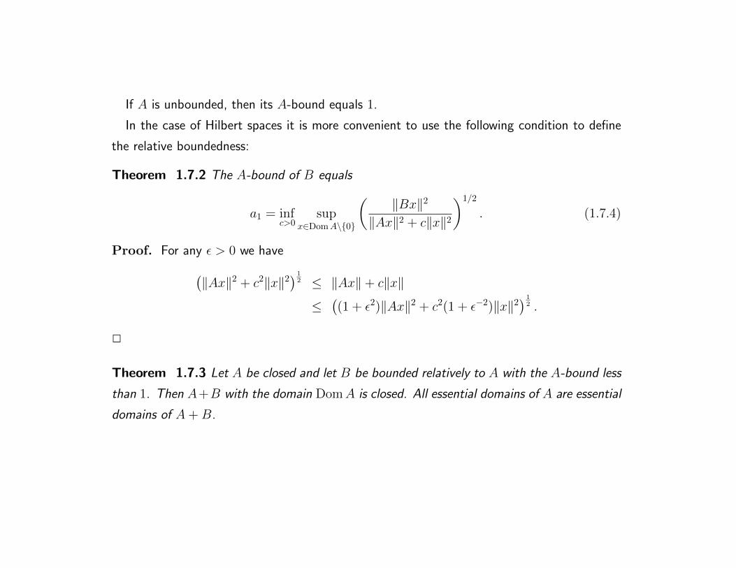
If A is unbounded, then its A-bound equals 1.
In the case of Hilbert spaces it is more convenient to use the following condition to define
the relative boundedness:
Theorem 1.7.2 The A-bound of B equals
a1 = infc>0
supx∈DomA\0
(‖Bx‖2
‖Ax‖2 + c‖x‖2
)1/2
. (1.7.4)
Proof. For any ε > 0 we have(‖Ax‖2 + c2‖x‖2
) 12 ≤ ‖Ax‖+ c‖x‖
≤((1 + ε2)‖Ax‖2 + c2(1 + ε−2)‖x‖2
) 12 .
2
Theorem 1.7.3 Let A be closed and let B be bounded relatively to A with the A-bound less
than 1. Then A+B with the domain DomA is closed. All essential domains of A are essential
domains of A+B.

Proof. We know that
‖Bx‖ ≤ a‖Ax‖+ b‖x‖
for some a < 1 and b. Hence
‖(A+B)x‖+ ‖x‖ ≤ (1 + a)‖Ax‖+ (1 + b)‖x‖
and
(1− a)‖Ax‖+ ‖x‖ ≤ ‖Ax‖ − ‖Bx‖+ (1 + b)‖x‖ ≤ ‖(A+B)x‖+ (1 + b)‖x‖.
Hence the norms ‖Ax‖+ ‖x‖ and ‖(A+B)x‖+ ‖x‖ are equivalent on DomA. 2
In particular, every bounded operator with domain containing DomA is bounded relatively
to A.
Proposition 1.7.4 Suppose that X = Y . Then we have the following seemingly different

definition of the A-bound of B:
a1 := infµ∈C
infc>0
supx∈DomA\0
‖Bx‖‖(A− µ)x‖+ c‖x‖
.
Proof. It suffices to note that
‖Ax‖+ c‖x‖ ≤ ‖(A− µ)x‖+ (µ+ c)‖x‖.
2
Theorem 1.7.5 Suppose that A,C are two operators with the same domain DomA =
DomC = D satisfying
‖(A− C)x‖ ≤ a(‖Ax‖+ ‖Cx‖) + b‖x‖
for some a < 1. Then
(1) A is closed on D iff C is closed on D.

(2) D is an essential domain of Acl iff it is an essential domain of Ccl.
Proof. Define B := C −A and F (t) := A+ tB with the domain D. For 0 ≤ t ≤ 1, we have
‖Bx‖ ≤ a(‖Ax‖+ ‖Cx‖) + b‖x‖
= a (‖(F (t)− tB)x‖+ ‖(F (t) + (1− t)B)x‖) + b‖x‖
≤ 2a‖F (t)x‖+ a‖Bx‖+ b‖x‖
Hence
‖Bx‖ ≤ 2a
1− a‖F (t)x‖+
b
1− a‖x‖.
Therefore, if |s| < 1−a2a and t, t+ s ∈ [0, 1], then F (t+ s) is closed iff F (t) is closed. 2
1.8 Invertible unbounded operators
Let A be an operator from X to Y .
Definition 1.8.1 We say that an operator A is invertible (or boundedly invertible) iff A−1 ∈

B(Y ,X ).
Note that we do not demand that A be densely defined. However, if A is invertible, then
necessarily RanA = Y .
The following criterion for the invertibility is obvious:
Proposition 1.8.2 Let C ∈ B(Y ,X ) be such that RanC ⊂ DomA and AC = 1l. Then A
is invertible and C = A−1.
Theorem 1.8.3 (Closed range theorem) Let A be closed. Suppose that for some c > 0
‖Ax‖ ≥ c‖x‖, x ∈ DomA. (1.8.5)
Then RanA is closed. If RanA = Y , then A is invertible and
‖A−1‖ ≤ c−1. (1.8.6)
Proof. Let yn ∈ RanA and yn → y. Let Axn = yn. Then xn is a Cauchy sequence. Hence
there exists limn→∞ xn := x. But A is closed, hence Ax = y. Therefore, RanA is closed. 2

Corollary 1.8.4 For an operator A, suppose that for some c > 0 (1.8.5) holds.
(1) Let A be closable. Then (1.8.5) holds for Acl as well.
(2) Let A be closed and RanA be dense in Y . Then A is invertible and ‖A−1‖ ≤ c−1.
Theorem 1.8.5 Let A be invertible and DomB ⊃ DomA.
(1) B has the A-bound less than ‖BA−1‖.
(2) If ‖BA−1‖ < 1, then A+B with the domain DomA is closed, invertible and
(A+B)−1 =∞∑j=0
(−1)jA−1(BA−1)j.
Proof. By the estimate
‖Bx‖ ≤ ‖BA−1‖‖Ax‖, x ∈ DomA,
we see that B has the A-bound less than or equal to ‖BA−1‖. This proves (1).

Assume now that ‖BA−1‖ < 1. Let
Cn :=n∑j=0
(−1)jA−1(BA−1)j.
Then limn→∞
Cn =: C exists.
Let y ∈ Y . Clearly, limn→∞
Cny = Cy.
(A+B)Cny = y + (−1)n(BA−1)n+1y → y.
But A+B is closed, hence Cy ∈ Dom(A+B) and (A+B)Cy = y. By Prop. 1.8.2, A+B
is invertible and C = (A+B)−1. 2
Theorem 1.8.6 Let A and C be invertible and DomC ⊃ DomA. Then
C−1 − A−1 = C−1(A− C)A−1.
Proposition 1.8.7 (1) Let B : X → Y be closed and bounded. Let A : Y → Z be closed.

Then AB is closed.
(2) Let C : Y → Z be closed and invertible. Let A : X → Y be closed. Then CA is closed.
1.9 Spectrum of unbounded operators
Let A be an operator on X . We define the resolvent set of A as
rsA := z ∈ C : z1l− A is invertible .
We define the spectrum of A as spA := C\rsA.
We say that x ∈ X is an eigenvector of A with eigenvalue λ ∈ C iff x ∈ DomA, x 6= 0
and Ax = λx. The set of eigenvalues is called the point spectrum of A and denoted sppA.
Clearly, sppA ⊂ spA.
Let C ∪ ∞ denote the Riemann sphere (the one-point compactification of C). The
extended resolvent set is defined as rsextA := rsA ∪ ∞ if A ∈ B(X ) and rsextA := rsA, if

A is unbounded. The extended spectrum is defined as
spextA = C ∪ ∞\rsextA.
If A ∈ B(X ), we set (∞− A)−1 = 0.
Theorem 1.9.1 (1) If rsA is nonempty, then A is closed.
(2) If z0 ∈ rsA, thenz : |z − z0| < ‖(z0 − A)−1‖−1 ⊂ rsA.
(3) ‖(z − A)−1‖ ≥ (dist(z, spA))−1.
(4) If A is bounded, then |z| > ‖A‖ is contained in rsA.
(5) spextA is a compact subset of C ∪ ∞.
(6) If λ, µ ∈ rsA, then
(z1 − A)−1 − (z2 − A)−1 = (z2 − z1)(z1 − A)−1(z2 − A)−1.
(7) If z ∈ rsA, thend
dz(z − A)−1 = −(z − A)−2.

(8) (z − A)−1 is analytic on rsextA.
(9) (z − A)−1 cannot be analytically extended to a larger subset of C ∪ ∞ than rsext(A).
(10) spext(A) 6= ∅
(11) Ran (z − A)−1 does not depend on z ∈ rsA and equals DomA.
(12) Ker(z − A)−1 = 0.
Proof. (1): If λ ∈ rs(A), then λ − A is invertible, hence closed. λ − A is closed iff A is
closed.
(2): For |z− z0| < ‖(z0−A)−1‖−1, we have ‖(z− z0)(z0−A)−1‖ < 1 Hence we can apply
Theorem 2.
By (2), dist(z0, spA) ≥ ‖(z0 − A)−1‖−1. This implies (3).
(4): We check that∞∑n=0
z−n−1An is convergent for |z| > ‖A‖ and equals (z − A)−1.
(5): By (2), spextA ∩ C = spA is closed in C. For bounded A, spextA is bounded by (4).
For unbounded A, ∞ ∈ spextA. So in both cases, spextA is closed inin C ∩ ∞.(6) follows from Thm 1.8.6. Note that it implies the continuity of the resolvent.

(7) follows from (6).
(8) follows from (7).
(9) follows from (3).
(10): For bounded A, (z − A)−1 is an analytic function tending to zero at infinity. Hence
it cannot be analytic everywhere, unless it is zero, which is impossible. For unbounded A,
∞ ∈ spextA.
(11) and (12) follow from (6). 2
Proposition 1.9.2 Suppose that rsA is non-empty and DomA is dense. Then DomA2 is
dense.
Proof. Let z ∈ rsA. (z − A)−1 is a bounded operator with a dense range and DomA is
dense. Hence (z−A)−1 DomA is dense. A(z−A)−1 DomA = (z−A)−1ADomA ⊂ DomA
Hence (z − A)−1 DomA ⊂ DomA2. 2
Theorem 1.9.3 Let A and B be operators on X with A ⊂ B, A 6= B. Then rsA ⊂ spB,
and hence rsB ⊂ spA.

Proof. Let λ ∈ rsA. Let x ∈ DomB\DomA. We have Ran (λ − A) = X , hence there
exists y ∈ DomA such that (λ − A)y = (λ − B)x. Hence (λ − B)y = (λ − B)x. Hence
λ 6∈ rsB. 2
1.10 Functional calculus
Let K ⊂ C ∪ ∞ be compact. By Hol(K) let us denote the set of analytic functions on a
neighborhood of K. It is a commutative algebra.
More precisely, let Hol(K) be the set of pairs (f,D), where D is an open subset of C∪∞containing K and f is an analytic function on D. We introduce the relation (f1,D1) ∼ (f2,D2)
iff f1 = f2 on a neighborhood of K contained D1 ∩ D2. We set Hol(K) := Hol(K)/ ∼.
Definition 1.10.1 Let A be an operator on X and f ∈ Hol(spextA). Let γ be a contour in a
domain of f that encircles spextA counterclockwise. We define
f(A) :=1
2πi
∫γ
(z − A)−1f(z)dz (1.10.7)

Clearly, the definition is independent of the choice of the contour.
Note that if spAext is the whole Riemann sphere (or equivalently spA = C), then the
functional calculus is trivial, since Hol(C∪∞) coincides with constant functions.
Theorem 1.10.2
Hol(spextA) 3 f 7→ f(A) ∈ B(X ) (1.10.8)
is a linear map satisfying
(1) fg(A) = f(A)g(A);
(2) 1(A) = 1l;
(3) If A ∈ B(X ), then id ∈ Hol(spextA) for id(z) = z and id(A) = A.
(4) If f(z) :=∑∞
n=0 fnzn is an analytic function defined by a series absolutely convergent in
a disk of radius greater than srA, then
f(A) =∞∑n=0
fnAn;

(5) (Spectral mapping theorem). spf(A) = f(spextA)
(6) g ∈ Hol(f(spextA))⇒ g f(A) = g(f(A)),
(7) ‖f(A)‖ ≤ cγ,A supz∈γ |f(z)|.
Proof. It is obvious that 1(A) = 1l. From the formula
(z − A)−1 =∞∑n=0
z−n−1An, |z| > sr(A),
we get that id(A) = A.
It is clear that f → f(A) is linear. Let us show that it is multiplicative. Let f1, f2 ∈Hol(spA). Choose a contour γ2 around the contour γ1, both in the domains of f1 and f2.
(2πi)−2∫γ1f1(z1)(z1 − A)−1dz1
∫γ2f2(z2)(z2 − A)−1dz2
= (2πi)−2∫γ1
∫γ2f1(z1)f2(z2)
((z1 − A)−1 − (z2 − A)−1
)(z2 − z1)
−1dz1dz2
= (2πi)−2∫γ1f1(z1)(z1 − A)−1dz1
∫γ2
(z2 − z1)−1f2(z2)dz2
+(2πi)−2∫γ2f2(z2)(z2 − A)−1dz2
∫γ1
(z1 − z2)−1f1(z1)dz1.
But ∫γ1
(z1 − z2)−1f1(z1)dz1 = 0,∫
γ2(z2 − z1)
−1f2(z2)dz2 = 2πif2(z1).
Thus
f1(A)f2(A) = f1f2(A). (1.10.9)
Let us prove the spectral mapping theorem. First we will show
spf(A) ⊂ f(spextA). (1.10.10)
If µ 6∈ f(spextA), then the function z 7→ f(z)−µ 6= 0 on spextA. Therefore, z 7→ (f(z)−µ)−1
belongs to Hol(spextA). Thus f(A)− µ is invertible and therefore, µ 6∈ spf(A). This implies
(1.10.10).
Let us now show
spf(A) ⊃ f(spextA). (1.10.11)
Let µ 6∈ spf(A). This clearly implies that f(A)− µ is invertible.
If µ does not belong to the image of f , then of course it does not belong to f(spextA). Let
us assume that µ = f(λ). Then the function
z 7→ g(z) := (f(z)− µ)(z − λ)−1
belongs to Hol(spextA). Hence g(A) is well defined as an element of B(X ). We check that
g(A)(f(A) − f(λ))−1 = (λ − A)−1. Hence λ 6∈ spextA. Thus µ 6∈ f(spA). Consequently,
(1.10.11) holds.
Let us show now (6). Notice that if w 6∈ f(spextA), then the function z 7→ (w− f(z))−1 is
analytic on a neighborhood of
(w − f(A))−1 =1
2πi
∫γ
(w − f(z))−1(z − A)−1dz.
We compute
g(f(A))
= 12πi
∫γ g(w)(w − f(A))−1dw
= 1(2πi)2
∫γ
∫γ g(w)(w − f(z))−1(z − A)−1dwdz
= 1(2πi)2
∫γ(z − A)−1dz
∫γ g(w)(w − f(z))−1dw
= 12πi
∫γ g(f(z))(z − A)−1dz.
2
1.11 Spectral idempotents
Let Ω be a subset of B ⊂ C∪∞. Ω will be called an isolated subset of B, if Ω∩(B\Ω)cl = ∅and Ωcl ∩ (B\Ω) = ∅ (or Ω is closed and open in the relative topology of B).
If B is in addition closed, then Ω is isolated iff both Ω and (B\Ω)cl are closed in C∪∞.Let Ω be an isolated subset of spextA. It is easy to see that we can find open non-intersecting

neighbohoods of Ω and spextA\Ω. Hence
1lΩ(z) :=
1 z belongs to a neighborhood of Ω,
0 z belongs to a neighborhood of spextA\Ω.
defines an element of Hol(spextA).
Clearly, 1l2Ω = 1lΩ. Hence 1lΩ(A) is an idempotent.
If γ is a counterclockwise contour around Ω outside of spextA\Ω then
1lΩ(A) =1
2πi
∫γ
(z − A)−1dz
This operator will be called the spectral idempotent of the operator A onto Ω.
spext(A∣∣Ran 1Ω(A)
)= spextA ∩ Ω.
If Ω1 and Ω2 are two isolated subsets of spextA, then
1lΩ1(A)1lΩ2
(A) = 1lΩ1∩Ω2(A)

1.12 Examples of unbounded operators
Example 1.12.1 Let I be an infinite set and (ai)i∈I be an unbounded complex sequence. Let
C0(I) be the space of sequences with a finite number of non-zero elements. For 1 ≤ p < ∞we define the operator
Lp(I) ⊃ C0(I) 3 x 7→ Ax ∈ Lp(I)
by the formula
(Ax)i = aixi.
(We can use C∞(I) instead of Lp(I), then p =∞ in the formulas below). Then the operator
A is unbounded and non-closed. Besides,
spp(A) = ai : i ∈ I,
spA = C.

The closure of A has the domain
DomAcl := (xi)i∈I ∈ Lp(I) :∑
i∈I |aixi|p <∞ (1.12.12)
We then havespp(Acl) = ai : i ∈ I,
spAcl = ai : i ∈ Icl.
To prove this let D be the rhs of (1.12.12) and x ∈ D. Then there exists a countable set I1 such
that i 6∈ I1 implies xi = 0. We enumerate the elements of I1: i1, i2, . . . . Define xn ∈ C0(I)
setting xnij = xij for j ≤ n and xni = 0 for the remaining indices. Then limn→∞ xn = x and
Axn → Ax. Hence, (x,Ax) : x ∈ D ⊂ (GrA)cl.
If xn belongs to (1.12.12) and (xn, Axn)→ (x, y), then xni → xi and aixni = (Axn)i → yi.
Hence yi = aixi. Using that y ∈ Lp(I) we see that x belongs to (1.12.12).
Example 1.12.2 Let p−1 + q−1 = 1, 1 < p ≤ ∞ and let (wi)i∈I be a sequence that does not

belong to Lq(I). Let C0(I) be as above. Define
Lp(I) ⊃ C0(I) 3 x 7→ 〈w|x〉 :=∑i∈I
xiwi ∈ C.
Then 〈w| is non-closable.
It is sufficient to assume that I = N and define vni := |wi|qwi(∑ni=1 |wi|q)
, i ≤ n, vni = 0, i > n.
Then 〈w|vn〉 = 1 and ‖vn‖p = (∑n
i=1 |wi|q)− 1q → 0. Hence (0, 1) belongs to the closure of
the graph of the operator.
1.13 Pseudoresolvents
Definition 1.13.1 Let Ω ⊂ C be open. Then the continuous function
Ω 3 z 7→ R(z) ∈ B(X )
is called a pseudoresolvent if
R(z1)−R(z2) = (z2 − z1)R(z1)R(z2). (1.13.13)

Evidently, if A is a closed operator and Ω ⊂ rsA, then Ω 3 z 7→ (z−A)−1 is a pseudoresolvent.
Proposition 1.13.2 Let Ω 3 z 7→ Rn(z) ∈ B(X ) be a sequence of pseudoresolvents and
R(z) := s− limn→∞
Rn(z). Then R(z) is a pseudoresolvent.
Theorem 1.13.3 Let Ω 3 z 7→ R(z) ∈ B(X ) be a pseudoresolvent. Then
(1) R := RanR(z) does not depend on z ∈ Ω.
(2) N := KerR(z) does not depend on z ∈ Ω.
(3) R(z) is an analytic function and
d
dzR(z) = −R(z)2.
(4) R(z) is a resolvent of a certain operator iff N = 0. The domain of this operator equals
R.
Proof. Let us prove (4)⇐. Fix z1 ∈ Ω. If N = 0, then every element of R can be uniquely
represented as R(z1)x, x ∈ X . Define AR(z1)x := −x+ z1R(z1)x. By formula (1.13.13) we
check that the definition of A does not depend on z1. 2

Chapter 2
One-parameter semigroups on Banach spaces
2.1 (M,β)-type semigroups
Let X be a Banach space.
Definition 2.1.1 [0,∞[3 t 7→ W (t) ∈ B(X ) is called a strongly continuous one-parameter
semigroup iff
(1) W (0) = 1l;
47
(2) W (t1)W (t2) = W (t1 + t2), t1, t2 ∈ [0,∞[;
(3) limt0
W (t)x = x, x ∈ X ;
(4) for some t0 > 0, ‖W (t)‖ < M , 0 ≤ t ≤ t0.
Remark 2.1.2 Using the Banach-Steinhaus Theorem one can show that (4) follows from the
remaining points.
Theorem 2.1.3 Let W (t) e a strongly continuous semigroup. Then
(1) Besides, there exist constants M , β such that
‖W (t)‖ ≤Meβt; (2.1.1)
(2) [0,∞[×X 3 (t, x) 7→ W (t)x ∈ X is a continuous function.
Proof. By (4), for t ≤ nt0 we have ‖W (t)‖ ≤ Mn. Hence, ‖W (t)‖ ≤ M exp( tt0 logM).
Therefore, (2.1.1) is satisfied.

Let tn → t and xn → x. Then
‖W (tn)xn −W (t)x‖ ≤ ‖W (tn)xn −W (tn)x‖+ ‖W (tn)x−W (t)x‖
≤Meβtn‖xn − x‖+Meβmin(tn,t)‖W (|t− tn|)x− x‖.
2
We say that the semigroup W (t) is (M,β)-type, if the condition (2.1.1) is satisfied.
Clearly, if W (t) is (M,β)-type, then W (t)e−βt is (M, 0)-type. Since W (0) = 1l, no semi-
groups (M,β) exist for M < 1.
2.2 Generator of a semigroup
If W (t) is a strongly continuous one-parameter semigroup, we define
DomA := x ∈ X : there exists limt0
t−1(W (t)x− x).

The operator A with the domain DomA is defined by the formula
Ax := limt0
t−1(W (t)x− x).
A will be called the generator of W (t). In the following theorem we show that an operator
cannot be the generator of more than one semigroup.
If W (t) is the semigroup generated by A, then we will write W (t) =: etA.
Theorem 2.2.1 (1) A is a closed densely defined operator;
(2) W (t) DomA ⊂ DomA and W (t)A = AW (t);
(3) If W1(t) and W2(t) are two different semigroups, then their generators are different.
Proof of Theorem 2.2.1 (2). Let x ∈ DomA. Then
lims0
s−1(W (s)− 1l)W (t)x = W (t) lims0
s−1(W (s)− 1l)x = W (t)Ax. (2.2.2)
Hence the limit of the left hand side of (2.2.2) exists. Hence W (t)x ∈ DomA and AW (t)x =
W (t)Ax. 2
Lemma 2.2.2 For x ∈ X put
Btx := t−1
∫ t
0
W (s)xds.
Then
(1) s− limt0
Bt = 1l.
(2) BtW (s) = W (s)Bt.
(3) For x ∈ DomA, ABtx = BtAx.
(4) If x ∈ X , then Btx ∈ DomA,
ABtx = t−1(W (t)x− x). (2.2.3)
(5) If limt0ABtx exists, then x ∈ DomA and the limit equals Ax.
Proof. (1) follows by
Btx− x = t−1
∫ t
0
(W (s)x− x)ds →t0
0.

(2) is obvious. (3) is proven as Theorem 2.2.1 (2). To prove (4) we note that
u−1(W (u)− 1l)Btx = t−1(W (t)− 1l)Bux →u0
t−1(W (t)x− x).
(5) follows from (4). 2
Proof of Theorem 2.2.1 (1) The density of DomA follows by Lemma 2.2.2 (1) and (3).
Let us show that A is closed. Let xn →n→∞
x and Axn →n→∞
y. Using the boundedness of
BtA = ABt we get
Bty = limn→∞
BtAxn = limn→∞
ABtxn = ABtx.
Hence
y = limt↓0
Bty = limt↓0
ABtx. (2.2.4)
By Lemma 2.2.2 (5), x ∈ DomA and (2.2.4) equals Ax. 2
Proposition 2.2.3 Let W (t) be a semigroup and A its generator. Then, for any x ∈ DomA

there exists a unique solution of
[0,∞[3 t 7→ x(t) ∈ DomA,d
dtx(t) = Ax(t), x(0) = x. (2.2.5)
(for t = 0 the derivative is right-sided). The solution is given by x(t) = W (t)x.
Proof. Let us show that x(t) := W (t)x solves (2.2.5), both for the left and right derivative:
u−1(W (t+ u)x−W (t)x) = W (t)u−1(W (u)− 1)x →u↓0
W (t)Ax = AW (t)x,
u−1(W (t− u)x−W (t)x) = W (t− u)u−1(W (u)− 1)x →u↓0
W (t)Ax = AW (t)x, 0 ≤ u ≤ t.
Let us show now the uniqueness. Let x(t) solve (2.2.5). Let y(s) := W (t− s)x(s). Then
d
dsy(s) = W (t− s)Ax(s)− AW (t− s)x(s) = 0
Hence y(s) does not depend on s. At s = t it equals x(t), and at s = 0 it equals W (t)x. 2
Proof of Theorem 2.2.1 (3) By Prop. 2.2.3 (2), W (t) is uniquely determined by A on
DomA. But W (t) is bounded and DomA is dense, hence W (t) is uniquely determined. 2

2.3 One-parameter groups
Definition 2.3.1 R 3 t 7→ W (t) ∈ B(X ) is called a strongly continuous one-parameter group
iff
(1) W (0) = 1l;
(2) W (t1)W (t2) = W (t1 + t2), t1, t2 ∈ R;
(3) limt→0
W (t)x = x, x ∈ X ;
(4) for some t0 > 0, ‖W (t)‖ < M , |t| ≤ t0.
Each 1-parameter group R 3 t 7→ W (t) consists of two semigroups:
[0,∞[3 t 7→ W (t), [0,∞[3 t 7→ W (−t).
If A is the generator of the former, then −A is the generator of the latter.
Conversely, if both A and −A generate semigroups, then they can be combined to form a
group.

2.4 Norm continuous semigroups
Theorem 2.4.1 (1) If A ∈ B(X ), then R 3 z 7→ etA =∞∑n=0
tn
n!An is a norm continuous
group and A is its generator.
(2) If a one-parameter semigroup W (t) is norm continuous, then its generator is bounded.
Proof. (1) follows by the functional calculus.
Let us show (2). W (t) is norm continuous, hence limt→0
Bt = 1l. Therefore, for 0 < t < t0
‖Bt − 1l‖ < 1.
Hence Bt is then invertible.
We know that for x ∈ DomA
t−1(W (t)− 1l)x = BtAx.

For 0 ≤ t < t0 we can write this as
Ax = t−1B−1t (W (t)− 1)x.
Hence ‖Ax‖ ≤ c‖x‖. 2
2.5 Essential domains of generators
Theorem 2.5.1 Let W (t) be a strongly continuous one-parameter semigroup and let A be
its generator. Let D ⊂ DomA be dense in X and W (t)D ⊂ D, t > 0. Then D is dense in
DomA in the graph topology—in other words, D is an essential domain of A.
Lemma 2.5.2 (1) For x ∈ X , ‖Btx‖DomA ≤ (Ct−1 + 1)‖x‖;
(2) For x ∈ DomA, limt↓0 ‖Btx− x‖DomA = 0;
(3) W (t) is a strongly continuous semi-group on DomA equipped with the graph norm.
(4) If D is a closed subspace in DomA invariant wrt W (t), then it is invariant also wrt Bt.

Proof. (1) follows by Lemma 2.2.2 (3).
(2) follows by Lemma 2.2.2 (1) and because B(t) commutes with A.
(3) follows from the fact that W (t) is a strongly continuous semigroup on X , preserves
DomA and commutes with A.
To show (4), note that Btx is defined using an integral involving W (s)x. W (s)x depends
continuously on s in the topology of DomA, as follows by (3). Hence this integral (as Rie-
mann’s integral) is well defined. Besides, Btx belongs to the closure of the space spanned by
W (s)x, 0 ≤ s ≤ t. 2
Proof of Theorem 2.5.1. Let x ∈ DomA, xn ∈ D and xn →n→∞
x in X . Let D be he
closure of D in DomA. Then Btxn ∈ D, by Lemma 2.5.2 (4). By Lemma 2.5.2 (1) we have
‖Btxn −Btx‖DomA ≤ Ct‖xn − x‖.
Hence Btx ∈ D. By Lemma 2.5.2 (2)
‖Btx− x‖DomA→t↓0
0.
Hence, x ∈ D. 2
2.6 Operators of (M,β)-type
Theorem 2.6.1 Let A be a densely defned operator. Then the following conditions are
equivalent:
(1) [β,∞[⊂ rs(A) and
‖(x− A)−m‖ ≤M |x− β|−m, m = 1, 2, . . . , x ∈ R, x > β
(2) z ∈ C : Rez > β ⊂ rs(A) and
‖(z − A)−m‖ ≤M |Rez − β|−m, m = 1, 2, . . . , z ∈ C, Rez > β.
Proof. It suffices to prove (1)⇒(2). Let (1) be satisfied. It suffices to assume that β = 0.

Let z = x+ iy. Then for t > 0
(z − A)−m = (x+ t− A)m(1l + (iy − t)(x+ t− A)−1)−m
=∞∑j=0
(x+ t− A)−m−j(iy − t)j(−mj
).
Using the fact that∣∣∣( −m
j
)∣∣∣ = (−1)j
(−mj
)we get
‖(z − A)−m‖ ≤M∞∑j=0
|x+ t|−m−j(−1)j|iy − t|j(−mj
)= M |x+ t|m
(1− |iy−t|x+t
)−m= M(x+ t− |iy − t|)−m →
t→∞Mx−m.
2
Definition 2.6.2 We say that an operator A is (M,β)-type, iff the conditions of Theorem

2.6.1 are satisfied.
Obviously, if A is of (M,β)-type, then A− β is of (M, 0)-type.
2.7 The Hille-Philips-Yosida theorem
Theorem 2.7.1 If W (t) is a semigroup of (M,β)-type, then its generator A is also of (M,β)-
type. Besides,
(z − A)−1 =
∫ ∞0
e−tzW (t)dt, Rez > β.
Proof. Set
R(z)x :=
∫ ∞0
e−ztW (t)xdt.

Let y = R(z)x. Then
u−1(W (u)− 1l)y
= −u−1ezu∫ u
0
e−ztW (t)xdt+ u−1(ezu − 1)
∫ ∞0
e−ztW (t)xdt →u0−x+ zy.
Hence y ∈ DomA and (z − A)R(z)x = x.
Suppose now that x ∈ Ker(z − A). Then xt := eztx ∈ DomA satisfies ddtxt = Axt. Hence
xt = W (t)x. But ‖xt‖ = eRezt‖x‖, which is impossible.
By the formula
(z − A)−m =
∫ ∞0
· · ·∫ ∞
0
e−z(t1+···+tm)W (t1 + · · ·+ tm)dt1 · · · dtm
we get the estimate
‖(z − A)−m‖ ≤∫ ∞
0
· · ·∫ ∞
0
Me−(z−β)(t1+···+tm)dt1 · · · dtm = M |z − β|−m.
2

Theorem 2.7.2 If A is an operator of (M,β)-type, then it is the generator of a semigroup
of (M,β)-type.
To simplify, let us assume that β = 0 (which does not restrict the generality). Then we
have the formula
etA = s− limn→∞
(1l− t
nA
)−n,∥∥∥∥∥etAx−
(1l− t
nA
)−nx
∥∥∥∥∥ ≤Mt2
2‖A2x‖, x ∈ DomA2.
Proof. Set
Vn(t) :=
(1l− t
nA
)−n.
Let us first show that
s− limt↓0
Vn(t) = 1l. (2.7.6)

To prove (2.7.6) it suffices to prove that
s− lims↓0
(1l− sA)−1 = 1l. (2.7.7)
We have (1l− sA)−1 − 1l = (s−1 − A)−1A. Hence for x ∈ DomA
‖(1l− sA)−1x− x‖ ≤Ms−1‖Ax‖,
which proves (2.7.7).
Let us list some other properties of Vn(t): for Ret > 0, Vn(t) is holomorphic, ‖Vn(t)‖ ≤M
andd
dtVn(t) = A
(1l− t
nA
)−n−1
.

To show that Vn(t)x is a Cauchy sequence for x ∈ Dom(A2), we compute
Vn(t)x− Vm(t)x = lims↓0 Vn(t− s)Vm(s)x− lims↑t Vn(t− s)Vm(s)x
= limε↓0∫ t−εε
ddsVn(t− s)Vm(s)x
= limε↓0∫ t−εε
(− V ′n(t− s)Vm(s) + Vn(t− s)V ′m(s)
)x
= limε↓0∫ t−εε
(sn −
t−sm
) (1l− t−s
n A)−n−1 (
1l− snA)−m−1
A2x.
Hence for x ∈ Dom(A2)
‖Vn(t)x− Vm(t)x‖ ≤ ‖A2x‖∫ t
0 |sm −
t−sn |M
2ds
= M 2( 1n + 1
m) t2
2 .
By the Proposition 1.9.2, Dom(A2) is dense in X . Therefore, there exists a limit uniform on
[0, t0]
s− limn→∞
Vn(t) =: W (t),
which depends strongly continuously on t.

Finally, let us show that W (t) is a semigroup with the generator A. To this end it suffices
to show that for x ∈ DomAd
dtW (t)x = AW (t)x. (2.7.8)
But x ∈ DomA
Vn(t+ u)x = Vn(t)x+
∫ t+u
t
A(
1l− s
nA)−1
Vn(s)xds
Hence passing to the limit we get
W (t+ u)x = W (t)x+
∫ t+u
t
AW (s)xds.
This implies (2.7.8). 2
2.8 Semigroups of contractions and their generators
Theorem 2.8.1 Let A be a closed operator on X . Then the following conditions are eqiva-
lent:

(1) A is a generator of a semigroup of contractions, i.e. ‖etA‖ ≤ 1, t ≥ 0.
(2) The operator A is of (1, 0)-type.
(3) ]0,∞[⊂ rs(A) and
‖(µ− A)−1‖ ≤ µ−1, µ ∈ R, µ > 0,
(4) z ∈ C : Rez > 0 ⊂ rs(A) and
‖(z − A)−1‖ ≤ |Rez|−1, z ∈ C, Rez > 0.
Proof. The equivalence of (1) and (2) is a special case of Theorems 2.7.1 and 2.7.2. The
implications (2)⇒(3) and (2)⇒(4) are obvious, the converse implications are easy. 2
Chapter 3
Unbounded operators on Hilbert spaces
3.1 Graph scalar product
Let V ,W be Hilbert spaces. Let A : V → W be an operator with domain DomA. It is natural
to treat DomA as a space with the graph scalar product
(v1|v2)A := (v1|v2) + (Av1|Av2).
Clearly, DomA is a Hilbert space with the graph scalar product iff A is closed.
67

3.2 The adjoint of an operator
Definition 3.2.1 Let A : V → W have a dense domain. Then w ∈ DomA∗, iff the functional
DomA 3 v 7→ (w|Av)
is bounded (in the topology of V). Hence there exists a unique y ∈ V such that
(w|Av) = (y|v), v ∈ V .
The adjoint of A is then defined by setting
A∗w = y.
Theorem 3.2.2 Let A : V → W have a dense domain. Then
(1) A∗ is closed.
(2) DomA∗ is dense in W iff A is closable.
(3) (RanA)⊥ = KerA∗.

(4) DomA ∩ (RanA∗)⊥ ⊃ KerA.
Proof. Let j : V ⊕W →W ⊕ V , j(v, w) := (−w, v). Note that j is unitary. We have
GrA∗ = j(GrA)⊥.
Hence GrA∗ is closed. This proves (1).
Let us prove (2).
w ∈ (DomA∗)⊥ ⇔ (0, w) ∈ (GrA∗)⊥ = j(GrA)⊥⊥
⇔ (w, 0) ∈ (GrA)⊥⊥ = (GrA)cl.

Proof of (3):
w ∈ KerA∗ ⇔ (A∗w|v) = 0, v ∈ V
⇔ (A∗w|v) = 0, v ∈ DomA
⇔ (w|Av) = 0, v ∈ DomA
⇔ w ∈ (RanA)⊥.
Proof of (4)
v ∈ KerA ⇔ (w|Av) = 0, w ∈ W
⇒ (w|Av) = 0, w ∈ DomA∗
⇔ (A∗w|v) = 0, w ∈ DomA∗
⇔ v ∈ (RanA∗)⊥.
Theorem 3.2.3 Let A : V → W be closable with a dense domain. Then
(1) A∗ is closed with a dense domain.
(2) A∗ = (Acl)∗.
(3) (A∗)∗ = Acl
(4) (RanA)⊥ = KerA∗. Hence A∗ is injective iff RanA is dense.
(5) (RanA∗)⊥ = KerA. Hence A is injective iff RanA∗ is dense.
Proof. (1) was proven in Theorem 3.2.2.
To see (2) note that
GrA∗ = j(GrA)⊥ = j((GrA)cl)⊥ = GrAcl∗.
To see (3) we use
Gr (A∗∗) = j−1(j(GrA)⊥
)⊥= (GrA)⊥⊥ = (GrA)cl.
(4) is proven in Theorem 3.2.2.
To prove (5) note that in the second line of the proof of Theorem 3.2.2 (4) we can use the
fact that DomA∗ is dense in W to replace ⇒ with ⇔. 2

3.3 Inverse of the adjoint operator
Theorem 3.3.1 Let A be densely defined, closed, injective and with a dense range. Then
(1) A−1 is densely defined, closed, injective and with a dense range.
(2) A∗ is densely defined, closed, injective and with a dense range.
(3) (A∗)−1 = (A−1)∗.
Proof. (1) and (2) sum up previously proven facts.
To prove (3), recall the maps τ, j : V ⊕W →W ⊕ V . We have
GrA∗ = j(GrA)⊥, GrA−1 = τ(GrA).
Hence
GrA−1∗ = j(τ(GrA))⊥ = τ−1(j(GrA)⊥) = GrA∗−1.
2
Theorem 3.3.2 Let A : V → W be densely defined and closed. Then the following conditions

are equivalent:
(1) A is invertible.
(2) A∗ is invertible.
(3) For some c > 0, ‖Av‖ ≥ c‖v‖, v ∈ V and ‖A∗w‖ ≥ c‖v‖, w ∈ W .
Proof. (1)⇒(2). Let A be invertible. Then A−1 ∈ B(W ,V). Hence, A−1∗ ∈ B(V ,W).
Clearly, the assumptions of Theorem 3.3.1 are satisfied, and hence A∗−1 = A−1∗. Therefore,
A∗−1 ∈ B(V ,W).
(1)⇐(2). A∗ is also densely defined and closed. Hence the same arguments as above apply.
It is obvious that (1) and (2) imply (3). Let us prove that (3)⇒(1). ‖A∗v‖ ≥ c‖v‖ implies
that KerA∗ = 0. Hence (RanA)⊥ is dense. This together with ‖Av‖ ≥ c‖v‖ implies that
RanA =W , and consequently, A is invertible. 2
Theorem 3.3.3 Let A : V → W be densely defined and closed. Then spext(A) = spext(A∗).
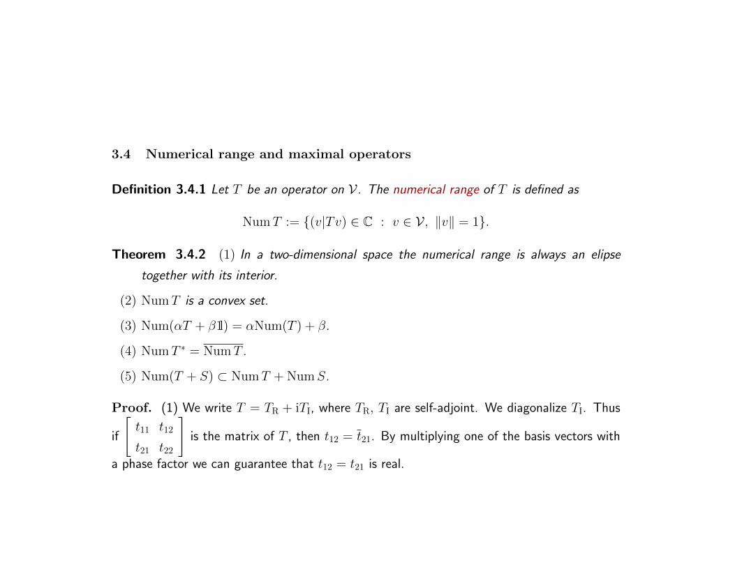
3.4 Numerical range and maximal operators
Definition 3.4.1 Let T be an operator on V . The numerical range of T is defined as
NumT := (v|Tv) ∈ C : v ∈ V , ‖v‖ = 1.
Theorem 3.4.2 (1) In a two-dimensional space the numerical range is always an elipse
together with its interior.
(2) NumT is a convex set.
(3) Num(αT + β1l) = αNum(T ) + β.
(4) NumT ∗ = NumT .
(5) Num(T + S) ⊂ NumT + NumS.
Proof. (1) We write T = TR + iTI, where TR, TI are self-adjoint. We diagonalize TI. Thus
if
[t11 t12
t21 t22
]is the matrix of T , then t12 = t21. By multiplying one of the basis vectors with
a phase factor we can guarantee that t12 = t21 is real.

Now T is given by a matrix of the form
c
[1 0
0 1
]+
[λ µ
µ −λ
]+ i
[γ 0
0 −γ
]
Any normalized vector up to a phase factor equals v = (cosα, eiφ sinα) and
(v|Tv)− c = λ cos 2α + µ cosφ sin 2α + iγ cos 2α =′: x+ iy. (3.4.1)
Now it is an elementary exercise to check that x+ iy are given by (3.4.1), iff they satisfy
(γx− λy)2 + µ2y2 ≤ γ2µ2.
(2) follows immediately from (1). 2
Theorem 3.4.3 (1) ‖(z − T )v‖ ≥ dist(z,NumT )‖v‖, v ∈ DomT .
(2) If T is a closed operator and z ∈ C\(NumT )cl, then z − T has a closed range.
(3) If z ∈ rsT\NumT , then ‖(z − T )−1‖ ≤ |dist(z,NumT )|−1.
(4) Let ∆ be a connected component of C\(NumT )cl. Then either ∆ ⊂ spT or ∆ ⊂ rsT .

Proof. To prove (1), take z 6∈ (NumT )cl. Recall that NumT is convex. Hence, replacing
T wih αT + β we can assume that z = iν and 0 ∈ (NumT )cl ⊂ Imz ≤ 0. Thus
ν = dist(iν,NumT ) and
‖(iν − T )v‖2 = (Tv|Tv)− iν(v|Tv) + iν(Tv|v) + |ν|2‖v‖2
= (Tv|Tv)− 2νIm(v|Tv) + |ν|2‖v‖2
≥ |ν|2‖v‖2.
(1) implies (2) and (3).
Let z0 ∈ rsT\NumT . By (3), if r = dist(z0,NumT ), then |z − z0| < r ⊂ rsT . This
proves (4). 2
Definition 3.4.4 An operator T is called maximal, if spT ⊂ (NumT )cl.
Clearly, if T is a maximal operator, and z 6∈ (NumT )cl, then
‖(z − T )−1‖ ≤ (dist(z,NumT ))−1.

If T is bounded, then T is maximal.
Theorem 3.4.5 Suppose that T is an operator and for any connected component ∆i of
C\(NumT )cl we choose λi ∈ ∆i. Then the following conditions are necessary and sufficient
for T to be maximal
(1) For all i, λi 6∈ spT ;
(2) T is closable and for all i, Ran (λi − T ) = V .
(3) T is closed and for all i, Ran (λi − T ) is dense in V .
(4) T is closed and for all i, Ker(λi − T ∗) = 0.
If K is a closed convex subset of C, then C\K is either connected or has two connected
components.

3.5 Dissipative operators
Definition 3.5.1 We say that an operator A is dissipative iff
Im(v|Av) ≤ 0, v ∈ DomA.
Equivalently, A is dissipative iff NumA ⊂ Imz ≤ 0.
Definition 3.5.2 A is maximally dissipative iff A is dissipative and spA ⊂ Imz ≤ 0.
Theorem 3.5.3 Let A be a densely defined operator. Then the following conditions are
equivalent:
(1) −iA is the generator of a strongly continuous semigroup of contractions.
(2) A is maximally dissipative.
Proof. (1) ⇒(2) We have
Re(v|e−itAv) ≤ |(v|e−itAv)| ≤ ‖v‖2.

HenceIm(v|Av) = Re(v| − iAv)
= Re limt0
t−1((v|e−itAv)− ‖v‖2
)≤ 0.
Hence A is dissipative.
We know that the generators of contractions satisfy Rez > 0 ⊂ rs(−iA).
(2)⇒(1) Let Rez > 0. We have
‖v‖‖(z + iA)v‖ ≥ |(v|(z + iA)v)|
≥ Re(v|(z + iA)v) ≥ Rez‖v‖2.
Hence, noting that z ∈ rs(−iA), we obtain ‖(z + iA)−1‖ ≤ Rez−1. Therefore, −iA is an
operator of the type (1, 0). 2
Theorem 3.5.4 Let A be dissipative. Then the following conditions are equivalent:
(1) A is maximally dissipative.
(2) A is closable and there exists z0 with Imz0 > 0 and Ran (z0 − A) = V .

(3) A is closed and there exists z0 with Imz0 > 0 and Ran (z0 − A) dense in V .
(4) A is closed and there exists z0 with Imz0 > 0 and Ker(z0 − A∗) = 0.
3.6 Hermitian operators
Definition 3.6.1 An operator A : V → V is hermitian iff
(Aw|v) = (w|Av), w, v ∈ DomA.
Equivalently, A is hermitian iff NumA ⊂ R.
If in addition A is densely defined, then it is hermitian iff A ⊂ A∗.
Remark 3.6.2 In a part of literature the term “symmetric” is used instead of “hermitian”.
Theorem 3.6.3 Let A be densely defined and hermitian. Then A is closable. Besides, one
of the following possibilities is true:
(1) spA ⊂ R.
(2) spA = Imz ≥ 0.

(3) spA = Imz ≤ 0.
(4) spA = C.
Proof. A is closable because A ⊂ A∗ and A∗ is closed. 2
Theorem 3.6.4 Let A be a densely defined operator. Then the following conditions are
equivalent:
(1) −iA is the generator of a strongly continuous semigroup of isometries.
(2) A is hermitian and spA ⊂ Imz ≤ 0.
Proof. (1)⇒(2): For v ∈ DomA,
0 = ∂t(e−itAv|e−itAv)
∣∣∣t=0
= −i(Av|v) + i(v|Av).
Hence A is hermitian.
Isometries are contractions. Hence, by Thm 2.8.1, spA ⊂ Imz ≤ 0.(2)⇒(1): By Thm 3.4.3, ‖(z + iA)−1‖ ≤ |Rez|−1, Rez > 0. Hence, by Thm 2.8.1, e−itA is
the generator of a strongly continuous contractive semigroup.

For v ∈ DomA,
0 = ∂t(e−itAv|e−itAv)
Hence, for v ∈ DomA, ‖e−itAv‖2 = ‖v‖2. In other words, e−itA is a group of isometries. 2
Theorem 3.6.5 Let A be hermitian. Then the following conditions are equivalent:
(1) spA ⊂ Imz ≤ 0.
(2) There exists z0 with Imz0 > 0 and Ran (z0 − A) = V .
(3) A is closed and there exists z0 with Imz0 > 0 and Ran (z0 − A) dense in V .
(4) A is closed and there exists z0 with Imz0 > 0 and Ker(z0 − A∗) = 0.
3.7 Self-adjoint operators
Definition 3.7.1 Let A be a densely defined operator on V . A is self-adjoint iff A∗ = A.
In other words, A is self-adjoint if for w ∈ W there exists y ∈ V such that
(y|v) = (w|Av), v ∈ DomA,

then w ∈ DomA and Aw = y.
Theorem 3.7.2 Every self-adjoint operator is hermitian and closed. If A ∈ B(V) , then it is
self-adjoint iff it is hermitian.
Theorem 3.7.3 Fix z± with ±Imz± > 0. Let A be hermitian. Then the following conditions
are necessary and sufficient for A to be self-adjoint:
(1) spA ⊂ R.
(2) z± 6∈ spA.
(3) Ran (z± − A) = V .
(4) A is closed and Ran (z± − A) is dense in V .
(5) A is closed and Ker(z± − A∗) = 0.
Theorem 3.7.4 Let z0 ∈ R. Let A be hermitian and z0 6∈ NumA. Then the following
conditions are sufficient for A to be self-adjoint:
(1) z0 6∈ spA.
(2) Ran (z0 − A) = V .
(3) A is closed and Ran (z0 − A) is dense in V .
(4) A is closed and Ker(z0 − A∗) = 0.
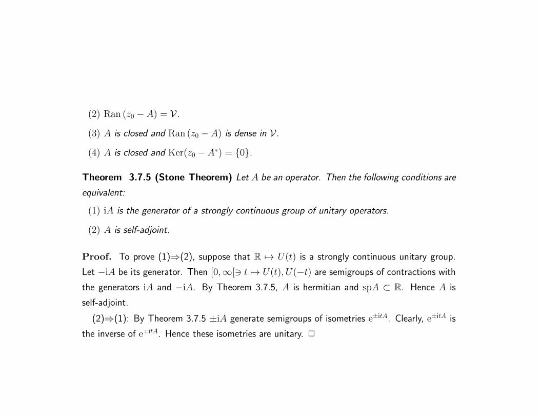
Theorem 3.7.5 (Stone Theorem) Let A be an operator. Then the following conditions are
equivalent:
(1) iA is the generator of a strongly continuous group of unitary operators.
(2) A is self-adjoint.
Proof. To prove (1)⇒(2), suppose that R 7→ U(t) is a strongly continuous unitary group.
Let −iA be its generator. Then [0,∞[3 t 7→ U(t), U(−t) are semigroups of contractions with
the generators iA and −iA. By Theorem 3.7.5, A is hermitian and spA ⊂ R. Hence A is
self-adjoint.
(2)⇒(1): By Theorem 3.7.5 ±iA generate semigroups of isometries e±itA. Clearly, e±itA is
the inverse of e∓itA. Hence these isometries are unitary. 2

3.8 Spectral theorem
Definition 3.8.1 Recall that B ∈ B(V) is called normal if B∗B = BB∗.
Let us recall one of the versions of the spectral theorem for bounded normal operators.
Let X be a Borel subset of C. Let M(X) denote the space of measurable functions on X
with values in C. For f ∈ M(X) we set f ∗(x) := f(x), x ∈ X. In particular, the function
X 3 z 7→ id(z) := z belongs to M(X).
L∞(X) will denote the space of bounded measurable functions on X.
Theorem 3.8.2 Let B be a bounded normal operator on V . Then there exists a unique linear
map
L∞(spB) 3 f 7→ f(B) ∈ B(V)
such that 1(B) = 1l, id(B) = B, fg(B) = f(B)g(B),
f(B)∗ = f ∗(B), ‖f(B)‖ ≤ sup |f |,if fn → f pointwise and |fn| ≤ c then s− lim
n→∞fn(B)→ f(B).
Above, all functions f, fn, g ∈ L∞(spB).

Theorem 3.8.3 Let B be a bounded normal operator B. Let f ∈M(spB). Set
fn(x) :=
f(x) |f(x)| ≤ n,
0, |f(x)| > n.
Dom(f(B)) = v ∈ V : sup ‖fn(B)v‖ <∞.
Then for v ∈ DomB there exists the limit
f(B)v := limn→∞
fn(B)v,
which defines a closed normal operator.
Let now A be a (possibly unbounded) self-adjoint operator on V .
Theorem 3.8.4 Then U := (A+ i)(A− i)−1 is a unitary operator with
spU = (spextA+ i)(spextA− i)−1.

Proof. Using the fact that A is hermitian, for v ∈ DomA we check that
‖(A± i)v‖2 = ‖Av‖2 + ‖v‖2.
Therefore, (A± i) : DomA → V are isometric. Using Ran (A± i) = V we see that they are
unitary. Hence so is (A+ i)(A− i)−1.
The location of the spectrum of U follows from
(z − U)−1 = (A− i)−1(z − 1)−1(A− i(z + 1)(z − 1)−1
)−1
.
2
U is unitary, hence normal. If f is a measurable function on spA, we define
f(A) := g(U),
where g(z) = f(i(z + i)(z − 1)−1).

Theorem 3.8.5 The map
M(spA) 3 f 7→ f(A) ∈ B(V)
is linear and satisfies 1(A) = 1l, id(A) = A, fg(A) = f(A)g(A),
f(A)∗ = f(A), ‖f(A)‖ ≤ sup |f |,where f, g ∈M(spA),
Definition 3.8.6 A possibly unbounded densely defined operator A is called normal if DomA =
DomA∗ and
‖Av‖2 = ‖A∗v‖, v ∈ DomA.
One can extend Thm 3.8.5 to normal unbounded operators in an obvious way.
Proposition 3.8.7 Let A be normal. Then the closure of the numerical range is the convex
hull of its spectrum.
Proof. We can write A =∫λdE(λ), where E(λ) is a spectral measure. Then for ‖v‖ = 1,
(v|Av) is the center of mass of the measure (v|dE(λ)v). 2

3.9 Essentially self-adjoint operators
Definition 3.9.1 An operator A : V → V is essentially self-adjoint iff Acl is self-adjoint.
Theorem 3.9.2 (1) Every essentially self-adjoint operator is hermitian and closable.
(2) A is essentially self-adjoint iff A∗ is self-adjoint.
Theorem 3.9.3 Let A be hermitian. Fix z± ∈ C with ±Imz± > 0. Then the following
conditions are necessary and sufficient for A to be essentially self-adjoint:
(1) Ran (z+ − A) and Ran (z− − A) are dense in V .
(2) Ker(z+ − A∗) = 0 and Ker(z− − A∗) = 0.
Theorem 3.9.4 Let A be hermitian. Let z0 ∈ R\NumA. Then the following conditions are
sufficient for A to be essentially self-adjoint:
(1) Ran (z0 − A) is dense in V .
(2) Ker(z0 − A∗) = 0.

3.10 Rigged Hilbert space
Let V be a Hilbert space with the scalar product (·|·). Suppose that T is a self-adjoint operator
on V with T ≥ c0 > 0. Then DomT can equipped with the scalar product
(Tv|Tw), v, w ∈ DomT
is a Hilbert space embedded in V . We will prove a converse construction, that leads from an
embedded Hilbert space to a positive self-adjoint operator.
Let V∗ denote the space of bounded antilinear functionals on V . The Riesz lemma says that
V∗ is a Hilbert space naturally isomorphic to V .
Suppose that W is a Hilbert space contained and dense in V . We assume that for c0 > 0
(w|w)W ≥ c0(w|w), w ∈ W . (3.10.2)
Of course, W∗ is also a Hilbert naturally isomorphic to W . However, we do not want to use
this isomorphism.
Let J : W → V denote the embedding. By (3.10.2), it is bounded. Clearly J∗ : V →

W∗ (where we use the identification V ' V∗). We have KerJ∗ = (Ran J)⊥ = 0 and
(Ran J∗)⊥ = KerJ = 0. Hence J∗ is a dense embedding of V in W∗. Thus we obtain a
triplet of Hilbert spaces, sometimes called a rigged Hilbert space
W ⊂ V ⊂ W∗.
Theorem 3.10.1 There exists a unique positive injective self-adjoint operator T on V such
that DomT =W and
(w1|w2)W = (Tw1|Tw2), w1, w2 ∈ W . (3.10.3)
Proof. Without loss of generality we will assume that c0 = 1.
For v ∈ V , w ∈ W , we have
|(w|v)| ≤ ‖w‖‖v‖ ≤ ‖w‖W‖v‖.

By the Riesz lemma, there exists A : V → W such that
(w|v) = (w|Av)W , (3.10.4)
We treat A as an operator from V to V . A is bounded, because
‖Av‖2 ≤ ‖Av‖2W = (Av|Av)W = (Av|v) ≤ ‖Av‖‖v‖.
A is positive, (and hence in particular self-adjoint) because
(Av|v) = (Av|Av)W ≥ 0.
A has a zero kernel, because Av = 0 implies
0 = (w|Av)V = (w|v), v ∈ DomW ,
and W is dense.

Thus T := A−1/2 defines a positive self-adjoint operator ≥ 1l. We have
(w|y)W = (w|T 2y), w ∈ W , y ∈ DomT 2 = RanA.
Using the lemma below, with two embedded Hilbert spaces W and DomT having a common
dense subspace DomT 2, we obtain W = DomT and the equality (3.10.3). 2
Lemma 3.10.2 Let W+,W− be two Hilbert spaces embedded in a Hilbert space V . Suppose
that their norms satisfy
‖w‖ ≤ ‖w‖+, w ∈ W+, ‖w‖ ≤ ‖w‖−, w ∈ W−.
Let D ⊂ W+ ∩W− be dense both in W+ and in W−. Suppose ‖ · ‖+ = ‖ · ‖− in D. Then
W+ =W− and ‖ · ‖+ = ‖ · ‖−.
Proof. Let w+ ∈ W+. There exists (wn) ⊂ D such that ‖wn − w+‖+ → 0. This implies
‖wn − w+‖ → 0.
Besides wn is Cauchy in W− Hence there exists w− ∈ W− such that ‖wn − w−‖− → 0.

This implies ‖wn−w−‖ → 0. Hence w+ = w−. Besides, ‖w+‖+ = lim ‖wn‖+ = lim ‖wn‖− =
‖w−‖−.
Thus W+ ⊂ W− and in W+ the norm ‖ · ‖+ coincides with the norm ‖ · ‖−. 2
By functional calculus for self-adjoint operators we can define S := T 2. Clearly, T =√S
and
(v|Sw) = (v|w)W , v ∈ Dom√S, w ∈ DomS.
We will say that the operator S is associated with the sesquilinear form (·|·)W .
3.11 Polar decomposition
Let A be a densely defined closed operator. Let S+ 1 be the positive operator associated with
the sesquilinear form
(Av|Aw) + (v|w), v, w ∈ DomA.
Theorem 3.11.1 S = A∗A.

In order to prove this theorem, introduce V1 = (1l + T )−1V and V−1 = (1l + T )V , so that
V1 = DomA and V−1 = V∗1 . Denote by A(1) the operator A treated as an operator V1 → V .
Clearly, A(1) is bounded, and so is A∗(1) : V → V−1.
Proposition 3.11.2 (1) DomA∗ = v ∈ V : A∗(1)v ∈ V.
(2) On DomA∗ the operators A∗ and A∗(1) coincide.
(3) DomT 2 = v ∈ DomA : Av ∈ DomA∗
(4) For v ∈ DomT 2, T 2v = A∗Av.
Proof. (1). Let w ∈ V . We have
w ∈ DomA∗ ⇔ |(w|Av)| ≤ C‖v‖, v ∈ DomA. (3.11.5)
But DomA = V1 and (w|Av) = (A∗(1)w|v). Hence, (3.11.5) is equivalent to
|(A∗(1)w|v)| ≤ C‖v‖, v ∈ DomA, (3.11.6)
which means A∗(1)w ∈ V .

In the proof of (3) we will use the operators T(1) and T ∗(1) defined analogously as A(1) and
A∗(1). We have
T ∗(1)T(1) = A∗(1)A(1). (3.11.7)
In fact, for v, w ∈ V1
(w|T ∗(1)T(1)v) = (T(1)w|T(1)v) = (A(1)w|A(1)v) = (w|A∗(1)A(1)v).
Now
DomT 2 = v ∈ V1 : T ∗(1)T(1)v ∈ V by spectral theorem
= v ∈ V1 : A∗(1)A(1)v ∈ V by (3.11.7)
= v ∈ V1 : A(1)v ∈ DomA∗ by (1).
2
Theorem 3.11.3 Let A be closed. Then there exist a unique positive operator |A| and a
unique partial isometry U such that KerU = KerA and A = U |A|. We have then RanU =

RanAcl.
Proof. The operator A∗A is positive. By the spectral theorem, we can then define
|A| :=√A∗A.
On Ran |A| the operator U is defined by
U |A|v := Av.
It is isometric, because
‖|A|v‖2 = (v||A|2v) = (v|A∗Av) = ‖Av‖2,
and correctly defined. We can extend it to (Ran |A|)cl by continuity. On Ker|A| = (Ran |A|)cl,
we extend it by putting Uv = 0. 2

3.12 Scale of Hilbert spaces I
Let A be a positive self-adjoint operator on V with A ≥ 1. We define the family of Hilbert
spaces Vα, α ∈ R as follows.
For α ≥ 0, we set Vα := RanA−α = DomAα with the scalar product
(v|w)α := (v|A2αw).
Clearly, for 0 ≤ α ≤ β we have the embedding Vα ⊃ Vβ.
For α ≤ 0 we set Vα := V∗−α, If α ≤ β ≤ 0 we have a natural inclusion Vα ⊃ Vβ.
Note that we have the identification V = V∗, hence both definitions give V0 = V .
Thus we obtain
Vα ⊃ Vβ, for any α ≤ β. (3.12.8)
Note that for α ≤ 0 V is embedded in Vα and for v, w ∈ V
(v|w)α =(v|A2αw
).

Moreover, V is dense in Vα.
Sometimes we will use a different notation: A−αV = Vα.
By restriction or extension, we can reinterpret the operator Aβ as a unitary operator
Aβ(−α) : AαV → Aα+βV .
If B is a self-adjoint operator, then we will use the notation 〈B〉 := (1 +B2)1/2. Clearly, B
gives rise to a bounded operator
B(α) : 〈B〉−αV → 〈B〉−α+1V .
Thus every self-adjoint operator can be interpreted in many ways, depending on β we choose.
The standard choice corresponding to β = 1
B(1) : DomB = 〈B〉−1V → V
can be called the “operator interpretation”.
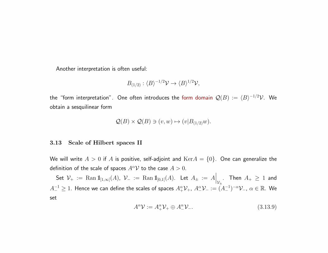
Another interpretation is often useful:
B(1/2) : 〈B〉−1/2V → 〈B〉1/2V ,
the “form interpretation”. One often introduces the form domain Q(B) := 〈B〉−1/2V . We
obtain a sesquilinear form
Q(B)×Q(B) 3 (v, w) 7→ (v|B(1/2)w).
3.13 Scale of Hilbert spaces II
We will write A > 0 if A is positive, self-adjoint and KerA = 0. One can generalize the
definition of the scale of spaces AαV to the case A > 0.
Set V+ := Ran 1l[1,∞[(A), V− := Ran 1l[0,1[(A). Let A± := A∣∣∣V±
. Then A+ ≥ 1 and
A−1− ≥ 1. Hence we can define the scales of spaces Aα
+V+, Aα−V− := (A−1
− )−αV−, α ∈ R. We
set
AαV := Aα+V+ ⊕ Aα
−V−. (3.13.9)

If A is not bounded away from zero, then the scale (3.13.9) does not have the nested property
(3.12.8). However, for any α, β ∈ R, AαV ∩ AβV is dense in AαV . Again, we have a family
of unitary operators
Aβ(α) : AαV → Aα+βV .
3.14 Complex interpolation
Let us recall a classic fact from complex analysis:
Theorem 3.14.1 (Three lines theorem) Suppose that a function 0 ≤ Rez ≤ 1 3 z 7→f(z) ∈ C is continuous, bounded, analytic in the interor of its domain, and satisfies the bounds
|f(is)| ≤ c0,
|f(1 + is)| ≤ c1, s ∈ R. (3.14.10)
Then
|f(t+ is)| ≤ c1−t0 ct1, t ∈ [0, 1], s ∈ R. (3.14.11)

Theorem 3.14.2 Let A > 0 on V , B > 0 on W . Consider an operator C : V ∩ A−1V →W ∩B−1W that satisfies
‖Cv‖ ≤ c0‖v‖,
‖BCv‖ ≤ c1‖Av‖, v ∈ V ∩ A−1V .
(In other words, C is bounded as an operator V → W with the norm ≤ c0 and A−1V → B−1Wwith the norm ≤ c1.) Then, for 0 ≤ t ≤ 1,
‖BtCv‖ ≤ c1−t0 ct1‖Atv‖, (3.14.12)
and so C extends to a bounded operator
C : A−tV → B−tW ,
with the norm ≤ c1−t0 ct1.

Proof. Let w ∈ W ∩B−1W and v ∈ V ∩A−1V . The vector valued functions z 7→ Bzw and
z 7→ Azv are bounded on 0 ≤ Rez ≤ 1, and hence so is
f(z) := (Bzw|CAzv)
We have
|f(is)| ≤ c0‖w‖‖v‖,
|f(1 + is)| ≤ c1‖w‖‖v‖, s ∈ R.
Hence,
|f(t)| ≤ c1−t0 ct1‖w‖‖v‖, t ∈ [0, 1].
This implies (3.14.12), by the density of W ∩B−1W . 2

3.15 Relative operator boundedness
Let A be a closed operator and B an operator with DomB ⊃ DomA. Recall that the
(operator) A-bound of B is
a1 := infν>0
supv 6=0, v∈DomA
(‖Bv‖2
‖Av‖2 + ν2‖v‖2
) 12
. (3.15.13)
In a Hilbert space
‖Av‖2 + ν2‖v‖2 = ‖(A∗A+ ν2)1/2v‖2.
Therefore, (3.15.13) can be rewritten as
a1 = infν>0‖B(A∗A+ ν2)−1/2‖. (3.15.14)
If, moreover, A is self-adjoint, then, using the unitarity of (A2 + ν2)−1/2(±iν − A), we can
rewrite (3.15.14) as
a1 = infν 6=0‖B(iν − A)−1‖. (3.15.15)

Using Prop. 1.7.4 we obtain
a1 = infz∈rsA
‖B(z − A)−1‖. (3.15.16)
Theorem 3.15.1 (Kato-Rellich) Let A be self-adjoint, B hermitian. Let B be A-bounded
with the A−bound < 1. Then
(1) A+B is self-adjoint on DomA.
(2) If A is essentally self-adjoint on D, then A+B is essentially self-adjoint on D.
Proof. Clearly, A+B is hermitian on DomA. Moreover, for some ν, ‖B(±iν −A)−1‖ < 1.
Hence, iν − A−B and −iν − A−B are invertible. 2
3.16 Relative form boundedness
Assume first that A is a positive self-adjoint operator. Let B be a bounded operator from
DomA1/2 = (1l +A)−1/2V to (1l +A)1/2V . Note that B defines a bounded quadratic form on
Q(B) := (1l + A)−1/2VQ(B) 3 u, v 7→ (u|Bv).

Let us assume that this form is hermitian, that is
(u|Bv) = (v|Bu).
Definition 3.16.1 We say that B is form-bounded relatively to A iff there exist constants a,
b such that
|(v|Bv)| ≤ a(v|Av) + b(v|v), v ∈ DomA1/2. (3.16.17)
The infimum of a satisfying (3.16.17) is called the A-bound of B.
In other words: the A-form bound of B equals
a2 := infc>0
supv∈DomA1/2\0
(v|Bv)
(v|Av) + c(v|v).
This can be rewritten as
a2 = infc>0‖(A+ c)−1/2B(A+ c)−1/2‖.
Theorem 3.16.2 A is a positive self-adjoint operator. Let B have the form A-bound less
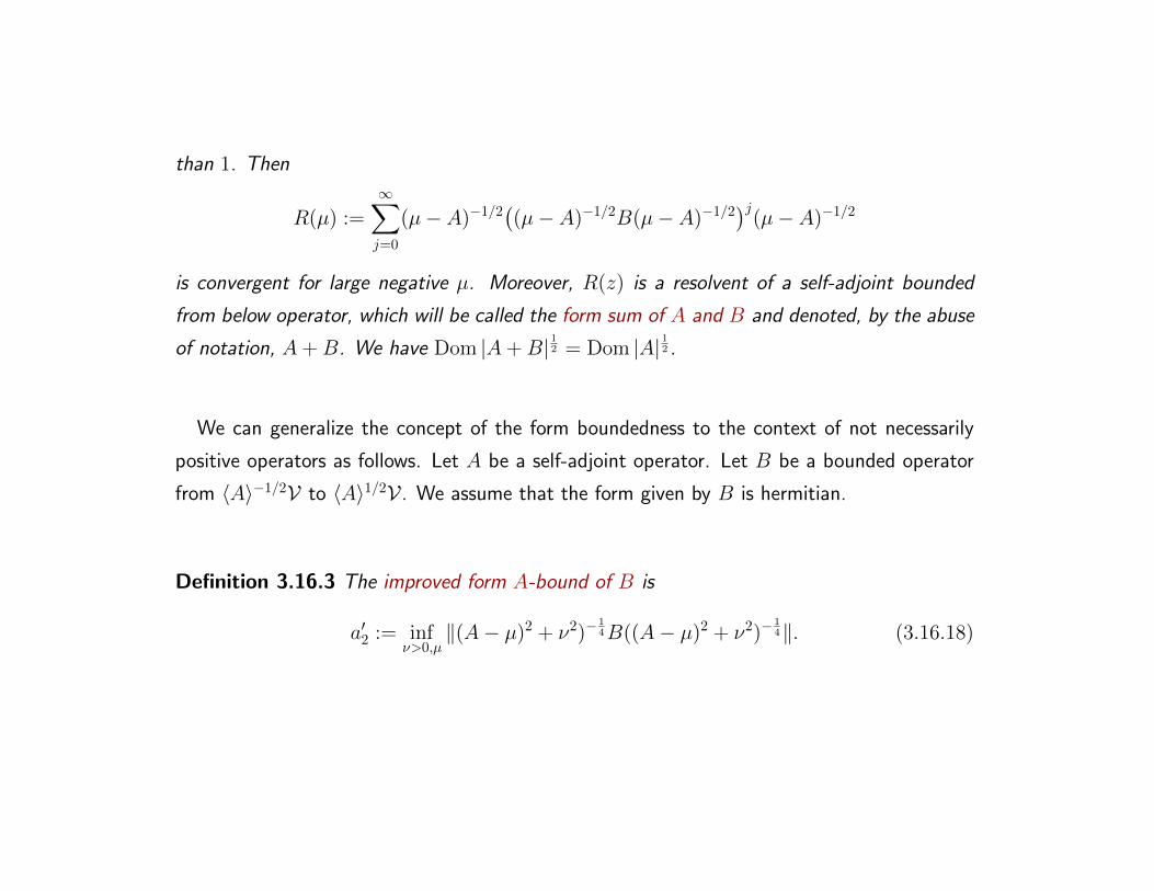
than 1. Then
R(µ) :=∞∑j=0
(µ− A)−1/2((µ− A)−1/2B(µ− A)−1/2
)j(µ− A)−1/2
is convergent for large negative µ. Moreover, R(z) is a resolvent of a self-adjoint bounded
from below operator, which will be called the form sum of A and B and denoted, by the abuse
of notation, A+B. We have Dom |A+B| 12 = Dom |A| 12 .
We can generalize the concept of the form boundedness to the context of not necessarily
positive operators as follows. Let A be a self-adjoint operator. Let B be a bounded operator
from 〈A〉−1/2V to 〈A〉1/2V . We assume that the form given by B is hermitian.
Definition 3.16.3 The improved form A-bound of B is
a′2 := infν>0,µ
‖(A− µ)2 + ν2)−14B((A− µ)2 + ν2)−
14‖. (3.16.18)

(3.16.18) can be rewritten as
a′2 = infν>0,µ
‖(µ+ iν − A)−12B(µ+ iν − A)−
12‖. (3.16.19)
Theorem 3.16.4 Let A be a self-adjoint operator. Let B have the improved A-form bound
less than 1. Then there exists open subsets in the upper and lower complex half-plane such
that the series
R(z) :=∞∑j=0
(z − A)−1/2((z − A)−1/2B(z − A)−1/2
)j(z − A)−1/2
is convergent. Moreover, R(z) is a resolvent of a self-adjoint operator, which will be called the
form sum of A and B and denoted, by the abuse of notation, A+B.
The form boundedness is stronger than the operator boundedness. Indeed, suppose that B
is a hermitian operator on V with DomB ⊃ DomA and
‖B((A− µ)2 + ν2
)1/2‖ ≤ a.
This means that B is bounded as an operator((A− µ)2 + ν2
)−1/2V → V and as an operator
V →((A − µ)2 + ν2
)1/2V , in both cases with norm ≤ a. By the complex interpolation, it is
bounded as an operator((A − µ)2 + ν2
)−1/4V →((A − µ)2 + ν2
)1/4V with norm ≤ a. In
particular, we have a′2 ≤ a1, where a1 is the operator A-bound and a′2 is the improved form
A-bound.
3.17 Self-adjointness of Schrodinger operators
The following lemma is a consequence of the Holder inequality:
Lemma 3.17.1 Let 1 ≤ p, q ≤ ∞ and 1p + 1
q = 1r . Then the operator of multiplication by
V ∈ Lp(Rd) is bounded as a map Lq(Rd)→ Lr(Rd) with norm equal to ‖V ‖q.
The following two lemmas follow from the Hardy-Littlewood-Sobolev inequality:
Lemma 3.17.2 The operator (1l−∆)−1 is bounded from L2(Rd) to Lq(Rd) in the following
cases:
(1) For d = 1, 2, 3 if 1∞ ≤
1q ≤
12 .

(2) For d = 4 if 1∞ < 1
q ≤12 .
(3) For d ≥ 5 if 12 −
2d ≤
1q ≤
12 .
Lemma 3.17.3 The operator (1l−∆)−12 is bounded from L2(Rd) to Lq(Rd) in the following
cases:
(1) For d = 1 if 1∞ ≤
1q ≤
12 .
(2) For d = 2 if 1∞ < 1
q ≤12 .
(3) For d ≥ 3 if 12 −
1d ≤
1q ≤
12 .
Proposition 3.17.4 Let V ∈ Lp + L∞(Rd),where
(1) for d = 1, 2, 3, p = 2,
(2) for d = 4, p > 2,
(3) for d ≥ 5, p = d2 .
Then the −∆-bound of V is zero. Hence −∆ + V (x) is self-adjoint on Dom(−∆).

Proof. We need to show that
limc→∞
V (x)(c−∆)−1 = 0, (3.17.20)
where (3.17.20) is understood as an operator on L2(Rd).
For any ε > 0 we can write V = V∞+Vp, where V∞ ∈ L∞(Rd), Vp ∈ Lp(Rd) and ‖Vp‖p ≤ ε.
Now
V (x)(c−∆)−1 = V∞(x)(c−∆)−1 + Vp(x)(c−∆)−1.
The first term has the norm ≤ ‖V∞‖∞c−1. Consider the second term. Let
1
q+
1
p=
1
2
‖Vp(x)Lq→L2 = ‖Vp‖p ≤ ε, and ‖(c−∆)−1L2→Lq‖ is uniformly finite for c > 1 by Lemma 3.17.3.
2
Proposition 3.17.5 Let V ∈ Lp + L∞(Rd),where

(1) for d = 1, p = 1,
(2) for d = 2, p > 1,
(3) for d ≥ 3, p = d2 .
Then the form −∆-bound of V is zero. Hence −∆ + V (x) can be defned in the sense of the
form sum with the form domain Dom(√−∆).
Proof. We need to show that
limc→∞
(c−∆)−1/2V (x)(c−∆)−1/2 = 0, (3.17.21)
where (3.17.21) is understood as an operator on L2(Rd). For any ε > 0 we can write V =
V∞ + Vp, where V∞ ∈ L∞(Rd), Vp ∈ Lp(Rd) and ‖Vp‖p ≤ ε. Now
(c−∆)−1/2V (x)(c−∆)−1/2 = (c−∆)−1/2V∞(x)(c−∆)−1/2
+(|Vp(x)|1/2(c−∆)−1/2
)∗sgnVp(x)|Vp(x)|1/2(c−∆)−1/2.

The first term has the norm ≤ ‖V∞‖∞c−1. Consider the second term. Let
1
q+
2
p=
1
2.
‖|Vp(x)|1/2Lq(Rd)→L2(Rd)‖ =
√‖Vp‖p ≤
√ε and ‖(c − ∆)
−1/2L2→Lq‖ is uniformly finite for c > 1 by
Lemma 3.17.3. 2

Chapter 4
Positive forms
4.1 Quadratic forms
Let V ,W be complex vector spaces.
Definition 4.1.1 a is called a sesquilinear form on W ×V iff it is a map
W ×V 3 (w, v) 7→ a(w, v) ∈ C
115

antilinear wrt the first argument and linear wrt the second argument.
If λ ∈ C, then λ can be treated as a sesquilinear form λ(w, v) := λ(w|v). If a is a form,
then we define λa by (λa)(w, v) := λa(w, v). and a∗ by a∗(v, w) := a(w, v). If a1 and a2 are
forms, then we define a1 + a2 by (a1 + a2)(w, v) := a1(w, v) + a2(w, v).
Suppose that V =W . We will write a(v) := a(v, v). We will call it a quadratic form. The
knowledge of a(v) determines a(w, v):
a(w, v) =1
4(a(w + v) + ia(w − iv)− a(w − v)− ia(w + iv)) . (4.1.1)
Suppose now that V ,W are Hilbert spaces. A form is bounded iff
|a(w, v)| ≤ C‖w‖‖v‖.
Proposition 4.1.2 (1) Let a be a bounded sesquilinear form on W × V . Then there exists
a unique operator A ∈ B(V ,W) such that
a(w, v) = (w|Av).

(2) If A ∈ B(V ,W), then (w|Av) is a bounded sesquilinear form on W ×V .
Proof. (2) is obvious. To show (1) note that w 7→ a(w|v) is an antilinear functional on W .
Hence there exists η ∈ W such that a(w, v) = (w|η). We put Av := η.
Theorem 4.1.3 Suppose that D,Q are dense linear subspaces of V ,W and a is a bounded
sesquilinear form on D ×Q. Then there exists a unique extension of a to a bounded form on
V ×W .
4.2 Sesquilinear quasiforms
Let V ,W be complex spaces. We say that t is a sesquilinear quasiform on W × V iff there
exist subspaces Doml t ⊂ W and Domr t ⊂ V such that
Domlt×Domrt 3 (w, v) 7→ t(w, v) ∈ C
is a sesquilinear map. From now on by a sesquilinear form we will mean a sesquilinear quasiform.
We define a form t∗ with the domains Doml t∗ := Domr t, Domr t
∗ := Doml t, by the formula

t∗(v, w) := t(w, v). If t1 are t2 forms, then we define t1 + t2 with the domain Doml(t1 + t2) :=
Doml t1∩Doml t1, Domr(t1 +t2) := Domr t1∩Domr t1 by (t1 +t2)(w, v) := t1(w, v)+t2(w, v).
We write t1 ⊂ t2 if Doml t1 ⊂ Doml t2, Domr t1 ⊂ Domr t2, and t1(w, v) = t2(w, v), w ∈Doml t1, v ∈ Domr t1.
From now on, we will usually assume that W = V and Doml t = Domr t and the latter
subspace will be simply denoted by Dom t. We will then write t(v) := t(v, v), v ∈ Dom t.
The numerical range of the form t is defined as
Numt := t(v) : v ∈ Dom t, ‖v‖ = 1.
We proved that Numt is a convex set.
With every operator T on V we can associate the form
t1(w, v) := (w|Tv), w, v ∈ DomT.
Clearly, Numt1 = NumT . If T is self-adjoint, we will however prefer to associate a different
form to it, see Theorem 4.5.1.

The form t is bounded iff Numt is bounded. Equivalently, |t(v)| ≤ c‖v‖2.
t is hermitian iff Numt ⊂ R. An equivalent condition: t(w, v) = t(v, w).
A form t is bounded from below, if there exists c such that
Numt ⊂ z : Rez > c.
A form t is positive if Numt ⊂ [0,∞[. In this section we develop the basics of the theory of
positive forms.
Note that many of the concepts and facts about positive forms generalize to hermitian
bounded from below forms. In fact, if t is bounded from below hermitian, then for some c ∈ Rwe have a positive form t + c. We leave these generalizations to the reader.
4.3 Closed positive forms
Let s be a positive form.

Definition 4.3.1 We say that s is a closed form iff Dom s with the scalar product
(w|v)s := (s + 1)(w, v), w, v ∈ Dom s, (4.3.2)
is a Hilbert space. We will then write ‖v‖s :=√
(v|v)s.
Clearly, the scalar product (4.3.2) is equivalent with
(s + c)(w, v), w, v ∈ Dom s,
for any c > 0.
Theorem 4.3.2 The form s is closed iff for any sequence (vn) in Dom s, if vn → v and
s(vn − vm)→ 0, then v ∈ Dom s and s(vn − v)→ 0.
Example 4.3.3 Let A be an operator. Then
(Aw|Av), w, v ∈ DomA,
is a closed form iff A is closed.

4.4 Closable positive forms
Let s be a positive form.
Definition 4.4.1 We say that s is a closable form iff there exists a closed form s1 such that
s ⊂ s1.
Theorem 4.4.2 (1) The form s is closable ⇔ for any sequence (vn) ⊂ Dom s, if vn → 0
and s(vn − vm)→ 0, then s(vn)→ 0.
(2) If s is closable, then there exists the smallest closed form s1 such that s ⊂ s1. We will
denote it by scl.
(3) Nums is dense in Numscl
Proof. (1) ⇒ follows immediately from Theorem 4.3.2.
To prove (1) ⇐, define s1 as follows: v ∈ Dom s1, iff there exists a sequence (vn) ⊂ Dom s
such that vn → v and s(vn − vm) → 0. From s(vn) ≤ (√s(v1) +
√s(vn − v1))
2 it follows
that(s(vn)
)is bounded. From |s(vn)− s(vm)| ≤
√s(vn − vm)
(√s(vn) +
√s(vn)
)it follows
that(s(vn)
)is a Cauchy sequence. Hence we can set s1(v) := lim
n→∞s(vn)

To show that the definition is correct, suppose that (wn) ∈ Dom s, wn → v and s(wn −wm) → 0. Then s(vn − wn − (vm − wm)) → 0 and vn − wn → 0. By the hypothesis we get
s(vn − wn) → 0. Hence, limn→∞
s(vn) = limn→∞
s(wn). Thus the definition of s1 does not depend
on the choice of the sequence vn. It is clear that s1 is a closed form containing s. Hence s is
closable.
To prove (2) note that the form s1 constructed above is the smallest closed form containg
s. 2
Example 4.4.3 Let A be an operator. Then
(Aw|Av), w, v ∈ DomA,
is closable iff A is a closable operator. Then
(Aclw|Aclv), w, v ∈ DomAcl
is its closure.
Definition 4.4.4 We say that a linear subspace Q is an essential domain of the form s if

(s∣∣∣Q×Q
)cl
= s.
4.5 Operators associated with positive forms
Let S be a self-adjoint operator. We define the form s as follows:
s(v, w) := (|S|1/2v|sgn(S)|S|1/2w), v, w ∈ Dom s := Dom |S|1/2.
We will say that s is the form associated with the operator S.
Theorem 4.5.1 (1) NumS is dense in Nums.
(2) If S is positive, then s is a closed positive form and DomS is its essential domain.
The next theorem describes the converse construction. It follows immediately from Thm
3.11.2.
Theorem 4.5.2 (Lax-Milgram Theorem) Let s be a densely defined closed positive form.

Then there exists a unique positive self-adjoint operator S such that
s(v, w) := (S1/2v|S1/2w), v, w ∈ Dom s := DomS1/2.
Proof. By Thm 3.10.1 applied to Dom s there exists a positive self-adjoint operator T such
that
s(v, w) := (Tv|Tw), v, w ∈ Dom s := DomT.
We set S := T 2. 2
We will say that S is the operator associated with the form s.
4.6 Perturbations of positive forms
Theorem 4.6.1 Let t1 and t2 be positive forms.
(1) t1 + t2 is also a positive form.
(2) If t1 and t2 are closed, then t1 + t2 is closed as well.

(3) If t1 and t2 are closable, then t1 + t2 is closable as well and (t1 + t2)cl ⊂ tcl
1 + tcl2 .
Definition 4.6.2 Let p, t be hermitian forms. Let t be positive. We say that p is t-bounded
iff Dom t ⊂ Dom p and
b := infc>0
supv∈Dom t
|p(v)|t(v) + c‖v‖2
<∞.
The number b is called the t-bound of p.
Theorem 4.6.3 Let t be positive and let p be t-bounded with the t-bound < 1. Then
(1) The form t + p (with the domain Dom t) is bounded from below.
(2) t is closed ⇔ t + p is closed.
(3) t is closable ⇔ t + p is closable, and then Dom(t + p)cl = Dom tcl.
Proof. Let us prove (1). For some b < 1, we have
(t + p)(v) ≥ t(v)− |p(v)| ≥ (1− b)t(v)− c‖v‖2. (4.6.3)
This proves that t + p is bounded from below.

To see (2) and (3), note that (4.6.3) and
(1 + b)t(v) + c‖v‖2 ≥ (t + p)(v)
prove that the norms ‖ · ‖t and ‖ · ‖t+p are equivalent. 2
4.7 Friedrichs extensions
Theorem 4.7.1 Let T be a positive densely defined operator. Then the form
t(w, v) := (w|Tv), w, v ∈ Dom t := DomT
is closable.
Proof. Suppose that wn ∈ DomT , wn → 0, limn,m→∞
t(wn − wm) = 0. Then
|t(wn)| ≤ |t(wn − wm, wn)|+ |t(wm, wn)|
≤√t(wn)
√t(wn − wm) + (wm|Twn).

For any ε > 0 there exists N such that for n,m > N we have t(wn − wm) ≤ ε2. Besides,
limm→∞
(wm|Twn) = 0. Therefore, for n > N ,
|t(wn)| ≤ ε|t(wn)|1/2.
Hence t(wn)→ 0. 2
Thus there exists a unique postive self-adjoint operator TFr associated with the form tcl.
The operator TFr is called the Friedrichs extension of T .
Clearly, DomT is then essential form domain of TFr. However in general it is not an essential
operator domain of T Fr. The theorem says nothing about essential operator domains.
For example, consider any open Ω ⊂ Rd. Note that C∞c (Ω) is dense in L2(Ω). The equation
(f | −∆g) =
∫∇f(x)∇g(x)dx, f ∈ C∞c (Ω)
shows that −∆ on C∞c (Ω) is a positive operator. Its Friedrichs extension is called the laplacian
on Ω with the Dirichlet boundary conditions.

If V is any positive bounded from below function we can consider ∆ + V (x) and define its
Friedrichs extension.

129

Chapter 5
Non-maximal operators
5.1 Defect indices
If V is a finite dimensional Hilbert space and V1,V2 its two subspaces such that V1∩V2 = 0,then we have the following obvious inequalities:
dimV1 + dimV2 ≤ dimV ,
dimV1 ≤ dimV⊥2 ,
dimV2 ≤ dimV⊥1 .
If dimV = ∞, then clearly the first inequality loses its interest. However the other two
inequalities, which are still true, may be interesting.
Let A be an operator on a Hilbert space V .
Theorem 5.1.1 dim Ran (z − A)⊥ = dim Ker(z − A∗) is a constant function on connected
components of C\(NumA)cl.
Proof. Let us show that if |z − z1| < dist(z,NumA), then
Ran (z − A) ∩ Ran (z1 − A)⊥ = 0. (5.1.1)
Let w ∈ Ran (z − A). Then there exists v ∈ DomA such that
w = (z − A)v
and ‖v‖ ≤ c‖w‖, where c =(dist(z,NumA)
)−1. If moreover, w ∈ Ran (z1 − A)⊥ =

Ker(z1 − A∗), then
0 =((z1 − A∗)w|v
)=(w|(z − A)v
)+ (z1 − z)(w|v)
= ‖w‖2 + (z − z1)(w|v).
But ∣∣‖w‖2 + (z1 − z)(w|v)∣∣ ≥ (1− |z1 − z|c)‖w‖2 > 0,
which is a contradiction and completes the proof of (5.1.1).
Now (5.1.1) implies that dim Ran (z − A)⊥ ≤ dim Ran (z1 − A)⊥. 2
5.2 Extensions of hermitian operators
Let A be closed hermitian.
Theorem 5.2.1 The so-called defect indices of A
n± := dim Ker(z − A∗), z ∈ C±

do not depend on z. Then A possesses a self-adjoint extension iff n+ = n−. Moreover, one of
the following possibilities is true:
(1) NumA 6= R.
(i) spA ⊂ R, n+ = n− = 0 and A is self-adjoint.
(ii) spA = C, n+ = n− > 0.
(2) NumA = R.
(i) spA ⊂ R, n+ = n− = 0, A is self-adjoint.
(ii) spA = Imz ≥ 0, n+ > 0, n− = 0, A is not self-adjoint.
(iii) spA = Imz ≤ 0, n+ = 0, n− > 0, A is not self-adjoint.
(iv) spA = C, n+ > 0, n− > 0, A is not self-adjoint.
Proof. The existence of self-adjoint extensions for n+ = n− follows from Theorem 5.2.3.
The remaining statements are essentially a special case of Theorem 5.1.1. 2

Definition 5.2.2 Define on DomA∗ the following scalar product:
(v|w)A∗ := (v|w) + (A∗v|A∗w)
and the following antihermitian form:
[v|w]A∗ := (A∗v|w)− (v|A∗w).
The A∗−closedness and the A∗−orthogonality is defined using the scalar product (·|·)A∗.
Theorem 5.2.3 (1) Every closed extension of A is a restriction of A∗ to an A∗−closed
subspace in DomA∗ containing DomA.
(2)
DomA∗ = DomA⊕Ker(A∗ + i)⊕Ker(A∗ − i)
and the components in the above direct sum are A∗-closed, A∗−orthogonal and
(w0 ⊕ w+ ⊕ w−|v0 ⊕ v+ ⊕ v−)A∗ = (w0|v0) + (Aw0|Av0) + 2(w+|v+) + 2(w−|v−),
[w0 ⊕ w+ ⊕ w−|v0 ⊕ v+ ⊕ v−]A∗ = 2i(w+|v+)− 2i(w−|v−).

Proof. (1) is obvious. In (2) the A∗−orthogonality and the A∗−closedness are easy.
Let w ∈ DomA∗ and
w ⊥A∗ DomA⊕Ker(A∗ + i).
In particular, for v ∈ DomA we have
0 = (A∗w|A∗v) + (w|v) = (A∗w|Av) + (w|v).
Hence A∗w ∈ DomA∗ and
A∗A∗w = −w.
Therefore,
(A∗ + i)(A∗ − i)w = 0.
Thus
(A∗ − i)w ∈ Ker(A∗ + i). (5.2.2)

If y ∈ Ker(A∗ + i), then
i(y|(A∗ − i)w) = (A∗y|A∗w) + (y|w) = (y|w)A∗ = 0
In particular, by (5.2.2) we can set y = (A∗ − i)w. We get w ∈ Ker(A∗ − i). 2
DomA belongs to the kernel of the antisymmetric form [·, ·]A∗. Therefore, in what follows
we restrict this form to
Vdef := Ker(A∗ + i)⊕Ker(A∗ − i).
We will write
Zper := v ∈ Vdef : [z, v]A∗ = 0, z ∈ Z.
We will say that a subspace Z of Vdef is A∗−isotropic iff [·|·]A∗ vanishes on Z and A∗-Lagrangian
if Zper = Z.
Every A∗−closed subspace of V containing DomA is of the form DomA ⊕ Z, where
Z ⊂ Vdef . If
A ⊂ B ⊂ A∗,

then the subspace Z corresponding to B will be denoted by ZB.
Theorem 5.2.4 (1) We have
ZB∗ = (ZB)per.
(2) B is hermitian iff ZB is A∗−isotropic iff there exists a partial isometry U : Ker(A∗+i)→Ker(A∗ − i) such that
Z := w+ ⊕ Uw+ : w+ ∈ RanU ∗U.
(3) B is self-adjoint iff ZB is A∗-Lagrangian iff there exists a unitary U : Ker(A∗ + i) →Ker(A∗ − i) such that
Z := w+ ⊕ Uw+ : w+ ∈ Ker(A∗ + i).
5.3 Extension of positive operators
(This subsection is based on unpublished lectures of S.L.Woronowicz).

Theorem 5.3.1 Let V = V0 ⊕ V1 and
B =
[B00 B01
B10 B11
]
be an operator in B(V) with B11 invertible. Then B is positive iff B11 ≥ 0, B01 = B∗10 and
B00 ≥ B01B−111 B10.
Proof. Let v0 ∈ V0, v1 ∈ V1. For vz =
[v0
v1
]. Then
0 ≤ (v|Bv) = (v0B00v0) + (v0|B01v1) + (v1|B10v0) + (v1|B11v1)
=(v0|(B00 −B01B
−111 B10)v0
)+ ‖B−1/2
11 B10v0 +B1/211 v1‖2
This proves ⇒.
Let us prove ⇐. The necessity of B11 ≥ 0 is obvious. Given v0, we can choose v1 =
−B−111 B10v0. This shows that B00 −B01B
−111 B10 has to be positive. 2

Suppose that G is hermitian, positive and closed. We would like to describe its positive
self-adjoint extensions. Thus we are looking for positive self-adjoint H such that G ⊂ H.
The operator G + 1l is injective and has a closed range. Define V1 := RanG and set
V0 := V⊥1 , so that V = V0⊕V1. Let A ∈ B(V1,V) be the left inverse of G+ 1l. We can write
it as
A =
[A01
A11
]We are looking for a bounded operator
(1l +H)−1 = B =
[B00 B01
B10 B11
]∈ B(V)
that extends A and 0 ≤ B ≤ 1l. Clearly, B11 = A11, B01 = A01, B10 = A∗01. By Theorem
5.3.1,
B00 ≥ B01B−111 B10,
1l00 −B00 ≥ B01(1l11 −B11)−1B10.

Thus we can choose any B00 ∈ B(V0) satisfying
1l00 − A01(1l11 − A11)−1A∗01 ≥ B00 ≥ A01A
−111 A
∗01.
This condition has two extreme solutions: The smallest A01A−111 A
∗01 yields the largest extension,
called the Friedrichs extension HFr. The largest 1l00−A01(1l11−A11)−1A∗01, gives the smallest
positive extension, called the Krein extension HKr. We have the following formula for both
extensions:
(1l +HFr)−1
:=(A
1/211 + A01A
−1/211
)(A
1/211 + A01A
−1/211
)∗,
1l− (1l +HKr)−1
:=((1l11 − A11)
1/2 − A01(1l11 − A11)−1/2
)((1l11 − A11)
1/2 − A01(1l11 − A11)−1/2
)∗.

141

Chapter 6
Aronszajn-Donoghue Hamiltonians and their
renormalization
6.1 Construction
Recall that the operators (h| and |h) are defined by
H 3 v 7→ (h|v := (h|v) ∈ C,
C 3 α 7→ |h)α := αh ∈ H.(6.1.1)

In particular, |h)(h| equals the orthogonal projection onto h times ‖h‖2.
Let H0 be a self-adjoint operator on H, h ∈ H and λ ∈ R.
Hλ := H0 + λ|h)(h|, (6.1.2)
is a rank one perturbation of H0. We will call (6.1.2) the Aronszajn Donoghue Hamiltonian.
We would like to describe how to define the Aronszajn-Donoghue Hamiltonian if h is not
necessarily a bounded functional on H. It will turn out that it is natural to consider 3 types of
h:
I. h ∈ H, II. h ∈ 〈H0〉1/2H \ H, III. h ∈ 〈H0〉H \ 〈H0〉1/2H, (6.1.3)
where 〈H0〉 := (1 +H20)1/2.
Clearly, in the case I Hλ is self-adjoint on DomH0. We will see that in the case II one
can easily define Hλ as a self-adjoint operator, but its domain is no longer equal to DomH0.
In the case III, strictly speaking, the formula (6.1.2) does not make sense. Nevertheless, it
is possible to define a renormalized Aronszajn-Donoghue Hamiltonian. To do this one needs

to renormalize the parameter λ. This procedure resembles the renormalization of the charge
in quantum field theory. In this case usually the parameter λ looses its meaning, so we will
abandon the notation Hλ. Instead, one can label the Hamiltonian by various parameters, which
we will put in brackets.
Lemma 6.1.1 In Case I with λ 6= 0, the resolvent of H equals
R(z) := (z −H)−1
= (z −H0)−1 − g(z)−1(z −H0)
−1|h)(h|(z −H0)−1, (6.1.4)
where
g(z) := −λ−1 + (h|(z −H0)−1h). (6.1.5)
defined for z 6∈ spH0.
Proof. We have
R(z)− (z −H0)−1 = λR(z)|h)(h|(z −H0)
−1
= λ(z −H0)−1|h)(h|R(z). (6.1.6)

Hence the range of (6.1.6) is C(z − H0)−1h, and the kernel is (z − H0)
−1h⊥. Therefore,
(6.1.6) has the form
−g(z)−1(z −H0)−1|h)(h|(z −H0)
−1 (6.1.7)
for some complex function g(z). Thus it remains to determine g(z) in (6.1.4). We insert
(6.1.4) into
λ(z −H0)−1|h)(h|R(z) = −g(z)−1(z −H0)
−1|h)(h|(z −H0)−1,
and we obtain the formula for g, sometimes called Krein’s formula. 2
For λ = 0, clearly
R0(z) = (z −H0)−1. (6.1.8)
The following theorem describes how to define the Aronszajn-Donoghue Hamiltonian also in
cases II and III:
Theorem 6.1.2 Assume that:
(A) h ∈ 〈H0〉1/2H, λ ∈ R ∪ ∞. Let Rλ(z) be given by (6.1.8) or (6.1.4) with gλ(z) given

by (6.1.5),
or
(B) h ∈ 〈H0〉H, γ ∈ R. Let R(γ)(z) be given by (6.1.4) where g(γ)(z) is the solution of∂zg(γ)(z) = −
(h|(z −H0)
−2h),
12
(g(γ)(i) + g(γ)(−i)
)= γ.
(6.1.9)
Then, for z ∈ C\spH0 such that g(z) 6= 0
(1) z 7→ R(z) is a pseudoresolvent (a function with values in bounded operators that fulfill
the first resolvent formula);
(2) KerR(z) = 0, unless h ∈ H and λ =∞;
(3) RanR(z) is dense in H, unless h ∈ H and λ =∞;
(4) R(z)∗ = R(z).
Hence, except for the case h ∈ H, λ = ∞, there exists a unique densely defined self-adjoint
operator H such that R(z) is the resolvent of H.
The initial condition in (6.1.9) can be called the renormalization condition. It is easy to solve

(6.1.9) obtaining
g(γ)(z) = γ +(h|((z −H0)
−1 +H0(1 +H20)−1
)h).
If g(β) = 0 and β 6∈ spH0, then H has an eigenvalue at β, and the corresponding eigenpro-
jection is
1β(H) = (h|(β −H0)−2h)−1(β −H0)
−1|h)(h|(β −H0)−1.
In Case I and II the function R ∪ ∞ 3 λ 7→ Hλ is increasing.
In Case III we rename H0 as H(∞).
6.2 Cut-off method
Another way to define H for the case h ∈ 〈H0〉H is the cut-off method. For Λ > 0 we define
hΛ := 1l[−Λ,Λ](H0)h, (6.2.10)
where 1l[−Λ,Λ](H0) is the spectral projection for H0 onto [−Λ,Λ] ⊂ R. Note that hΛ ∈ H.

We fix the running coupling constant by
−λ−1Λ := γ + (hΛ|H0(1 +H2
0)−1hΛ)
and set the cut-off Hamiltonian to be
HΛ := H0 + λΛ|hΛ)(hΛ|. (6.2.11)
Then the resolvent for HΛ is given by
RΛ(z) = (z −H0)−1 − gΛ(z)−1(z −H0)
−1|hΛ)(hΛ|(z −H0)−1, (6.2.12)
where
gΛ(z) := −λ−1Λ +
(hΛ|(z −H0)
−1hΛ
). (6.2.13)
Note that λΛ is chosen in such a way that the renormalization condition 12 (gΛ(i) + gΛ(−i)) = γ.
holds. The cut-off Hamiltonian converges to the renormalized Hamiltonian:
Theorem 6.2.1 Assume that h ∈ 〈H0〉H. Then limk→∞
RΛ(z) = R(z).

6.3 Extensions of hermitian operators
Let H0 be as above and h ∈ 〈H0〉H\H. (Thus we consider jointly Case II and III.) Define
Hmin to be the restriction of H0 to
Dom(Hmin) := v ∈ Dom(H0) = 〈H0〉−1H : (h|v) = 0.
Then Hmin is a closed densely defined Hermitian operator. Set Hmax := H∗min. Then
Dom(Hmax) = Span(
DomH0 ∪ (z0 −H0)−1h
),
where z0 ∈ rsH0. Note that Ker(Hmax ± i) is spanned by
v± := (±i−H0)−1h.
Thus the indices of defect of Hmin are (1, 1).
The operators H(γ) described in the previous subsection are self-adjoint extensions of Hmin.

To obtain H(γ) it suffices to increase the domain of Hmin by adding the vector
γ + (h|H0(1 +H20)−1h)
γ − i(h|(1 +H20)−1h)
(i−H0)−1h− γ + (h|H0(1 +H2
0)−1h)
γ + i(h|(1 +H20)−1h)
(i +H0)−1h,
If H(γ) has an eigenvalue β outside of spH0, then instead we can add the vector
(β −H0)−1h.
6.4 Positive H0
Let us consider the special case H0 > 0.
We can define the positive form hmin associated with Hmin:
hmin(v, v) = (v|Hminv) = (v|H0v),
v ∈ Dom(hmin) := DomHmin = v ∈ Dom(H0) : (h|v) = 0.
In Case II and III the form hmin is densely defined.
Clearly, g is analytic on C\[0,∞[. g restricted to ] −∞, 0[ is a decreasing function (in all

cases I, II and III). Therefore, H can possess at most one negative eigenvalue.
We distinguish subcases of Cases I, II and III
Case I iff h ∈ H;
Case Ia iff h ∈ DomH−1/20 ;
Case Ib iff h 6∈ DomH−1/20 .
Case II iff h ∈ (1 +H0)1/2H, h 6∈ H;
Case IIa iff (1 +H0)−1/2h ∈ Dom(1 +H0)
1/2H−1/20 ;
Case IIb iff (1 +H0)−1/2h 6∈ Dom(1 +H0)
1/2H−1/20 .
Case II iff h ∈ (1 +H0)H, h 6∈ (1 +H0)1/2H;
Case IIIa iff (1 +H0)−1h ∈ Dom(1 +H0)
1/2H−1/20 ;
Case IIIb iff (1 +H0)−1h 6∈ Dom(1 +H0)
1/2H−1/20 .

In Case Ia and IIa we set
λKr := −(h|H−10 h)−1. (6.4.14)
Note that λKr is negative. (In all other cases one could interpret (h|H−10 h) as +∞, and
therefore one can then set λKr := 0). We have
limx→−∞
g(x) = −λ−1, g(0) = −λ−1 + λ−1Kr .
Therefore, Hλ is positive for λKr ≤ λ ≤ ∞. For λ < λKr, Hλ has a single negative eigenvalue
β, which is the solution of
λ(h|(H0 − β)−1h) = −1. (6.4.15)
In Case IIa HλKris the Krein extension of Hmin and H∞ is the Friedrichs extension.
In Case Ib and IIb we have
limx→−∞
g(x) = −λ−1, g(0) = −∞.
Hλ is positive for 0 ≤ λ ≤ ∞. For λ < 0, Hλ has a single negative negative eigenvalue β,
which is the solution of (6.4.15). In Case IIb H0 is the Krein extension of Hmin and H∞ is its

Friedrichs extension.
In Case III we will use several kinds of parameters, always putting them in brackets. In
particular, it is natural to rename H0 and call it H(∞). It is the Friedrichs extension of Hmin.
In Case IIIa we have
limx→−∞
g(x) =∞, g(0) =: γ0,
where γ0 is a finite real number that can be used to parametrize H, so that
g(z) = γ0 −(h|(H0 − z)−1H−1
0 h)z.
H(γ0) is an increasing function of γ0. It is positive for 0 ≤ γ0. It has a single negative eigenvalue
at β solving
γ0 = (h|(H0 − β)−1H−10 h)β.
The Krein extension corresponds to γ0 = 0.
In Case IIIb
limx→−∞
g(x) =∞, g(0) = −∞.

A natural way to parametrize the Hamiltonian is by g(z0) for some fixed z0 ∈] −∞, 0[, say
γ−1 := g(−1). This yields
g(z) = γ−1 −(h|(H0 − z)−1(H0 + 1)−1h
)(z + 1).
H is an increasing function of γ−1 on R ∪ ∞. The Krein extension is H(∞) (and coincides
with the Friedrichs extension).
H(γ−1) has a single negative eigenvalue β for all γ−1 ∈ R. β is an increasing function of γ−1.
If we use the cut-off method in Case III, then λΛ 0. Thus we should think of λ as
infinitesimally small negative.

155

Chapter 7
Friedrichs Hamiltonians and their
renormalization
7.1 Construction
Let H0 be again a self-adjoint operator on the Hilbert space H. Let ε ∈ R and h ∈ H. The
following operator on the Hilbert space C⊕H is often called the Friedrichs Hamiltonian:
G :=
[ε (h||h) H0
]. (7.1.1)

We would like to describe how to define the Friedrichs Hamiltonian if h is not necessarily a
bounded functional on H. It will turn out that it is natural to consider 3 types of h:
I. h ∈ H, II. h ∈ 〈H0〉1/2H \ H, III. h ∈ 〈H0〉H \ 〈H0〉1/2H, (7.1.2)
Clearly, in the case I G is self-adjoint on C ⊕ DomH0. We will see that in the case II one
can easily define G as a self-adjoint operator, but its domain is no longer C ⊕ DomH0. In
the case III, strictly speaking, the formula (7.1.1) does not make sense. Nevertheless, it is
possible to define a renormalized Friedrichs Hamiltonian. To do this one needs to renormalize
the parameter ε. This procedure resembles the renormalization of mass in quantum field theory.
Let us first consider the case h ∈ H. As we said earlier, the operator G with DomG =
C⊕DomH0 is self-adjoint. It is well known that the resolvent of G can be computed exactly.
In fact, for z 6∈ spH0 define the analytic function
f(z) := ε+ (h|(z −H0)−1h). (7.1.3)

Then for z ∈ C\spH0, f(z) 6= z the resolvent Q(z) := (z −G)−1 is given by
Q(z) =
[0 0
0 (z −H0)−1
](7.1.4)
+(z − f(z)
)−1
1l (h|(z −H0)−1
(z −H0)−1|h) (z −H0)
−1|h)(h|(z −H0)−1
.Theorem 7.1.1 Assume that:
(A) h ∈ 〈H0〉1/2H, ε ∈ R. Let Q(z) be given by (7.1.4) with f(z) defined by (7.1.3),
or
(B) h ∈ 〈H0〉H, γ ∈ R. Let Q(z) be given by (7.1.4) with f(z) defined by∂zf(z) = −
(h|(z −H0)
−2h),
12
(f(i) + f(−i)
)= γ.
(7.1.5)
Then for all z ∈ C\spH0, f(z) 6= z :
(1) Q(z) is a pseudoresolvent;

(2) KerQ(z) = 0;
(3) RanQ(z) is dense in C⊕H;
(4) Q(z)∗ = Q(z).
Therefore, there exists a unique densely defined self-adjoint operator G such that Q(z) =
(z −G)−1.
Proof. Let z ∈ C\spH0, f(z) 6= z. It is obvious that Q(z) is bounded and satisfies (4). We
easily see that both in the case (A) and (B) the function f(z) satisfies
f(z1)− f(z2) = −(z1 − z2)(h|(z1 −H0)−1(z2 −H0)
−1|h). (7.1.6)
Direct computations using (7.1.6) show the first resolvent formula.
Let (α, f) ∈ C⊕H be such that (α, f) ∈ KerQ(z). Then
0 = (z − f(z))−1(α + (h|(z −H0)
−1f)), (7.1.7)
0 = (z −H0)−1f + (z −H0)
−1h(z − f(z))−1(α + (h|(z −H0)
−1f)). (7.1.8)
Inserting (7.1.7) into (7.1.8) we get 0 = (z −H0)−1f and hence f = 0. Now (7.1.7) implies
α = 0, so KerQ(z) = 0.
Using (2) and (4) we get (RanQ(z))⊥ = KerQ(z)∗ = KerQ(z) = 0. Hence (3) holds.
2
It is easy to solve (7.1.5):
f(z) := γ +(h|((z −H0)
−1 +H0(1 +H20)−1)h
)= γ +
(h|( i−z
2(z−H0)(i−H0) −i+z
2(z−H0)(−i−H0))h) (7.1.9)
7.2 The cut-off method
Let h ∈ 〈H0〉H and γ ∈ R. We can also use the cut-off method. For all Λ > 0 we define hΛ
as in (6.2.10), that is hΛ := 1l[−Λ,Λ](H0)h,. We set
εΛ := γ + (hΛ|H0(1 +H20)−1hΛ).
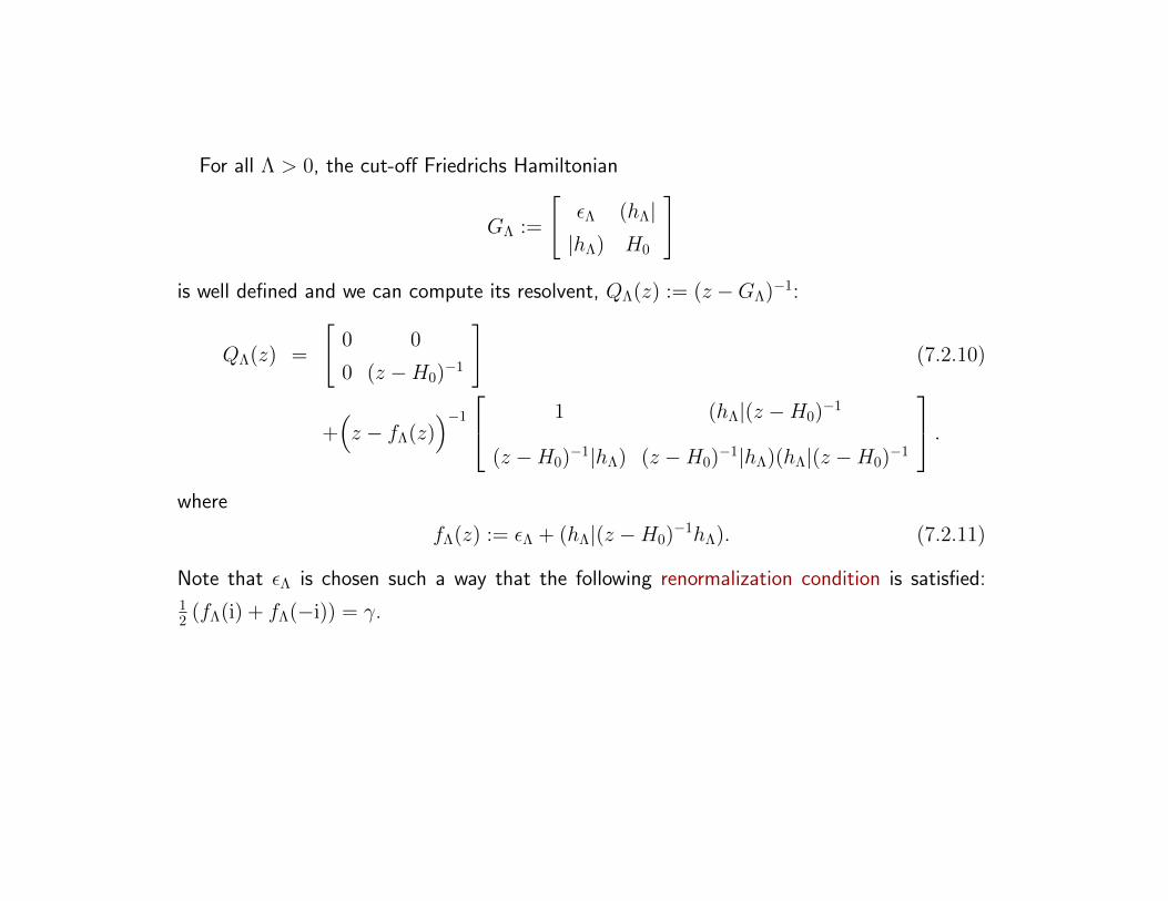
For all Λ > 0, the cut-off Friedrichs Hamiltonian
GΛ :=
[εΛ (hΛ||hΛ) H0
]
is well defined and we can compute its resolvent, QΛ(z) := (z −GΛ)−1:
QΛ(z) =
[0 0
0 (z −H0)−1
](7.2.10)
+(z − fΛ(z)
)−1
1 (hΛ|(z −H0)−1
(z −H0)−1|hΛ) (z −H0)
−1|hΛ)(hΛ|(z −H0)−1
.where
fΛ(z) := εΛ + (hΛ|(z −H0)−1hΛ). (7.2.11)
Note that εΛ is chosen such a way that the following renormalization condition is satisfied:12 (fΛ(i) + fΛ(−i)) = γ.

Theorem 7.2.1 Assume that h ∈ 〈H0〉H. Then limk→∞
QΛ(z) = Q(z), where Q(z) is given by
(7.1.4) and f(z) is given by (7.1.9). If H0 is bounded from below, then limk→∞
εΛ =∞.
Proof. The proof is obvious if we note that limk→∞‖(z − H0)
−1h − (z − H0)−1hΛ‖ = 0 and
limk→∞
fΛ(z) = f(z). 2
Thus the cut-off Friedrichs Hamiltonian is norm resolvent convergent to the renormalized
Friedrichs Hamiltonian.
7.3 Eigenvectors and resonances
Let β 6∈ spH0, If β = f(β) = 0 then G has an eigenvalue at β. The corresponding eigenpro-
jection equals
1lβ(G) = (1 + (h|(β −H0)−2|h))−1
[1 (h|(β −H0)
−1
(β −H0)−1|h) (β −H0)
−1|h)(h|(β −H0)−1
].
It may happen that C\spH0 3 z 7→ f(z) extends to an analytic multivalued function accross
some parts of spH0. Then so does the resolvent (z−G)−1 sandwiched between a certain class

of vectors, in particular, between
w :=
[1
0
](7.3.12)
(w∣∣(z −G)−1w
)= (z − f(z))−1.
It may happen that we obtain a solution of
f(β) = β
in this non-physical sheet of the complex plane. This gives a pole of the resolvent called a
resonance.
Suppose that we replace h with λh and ε with ε0 + λ2α and assume that we have Case I or
II with λ small.
Then if ε0 6∈ spH0, we have an approximate expression for the eigenvalue for small λ:
ελ = ε0 + λ2α + λ2(h|(ε0 −H0)−1h) +O(λ4).
If ε0 ∈ spH0, then the eigenvalue typically disappears and we obtain an approximate formula

for the resonance:
ελ = ε0 + λ2α + λ2(h|(ε0 + i0−H0)−1h) +O(λ4)
= ε0 + λ2α + λ2(h|P(ε0 −H0)−1h)− λ2iπ(h|δ(H0)h) +O(λ4).
Suppose now that ε0 = 0. Then we have the weak coupling limit:
limλ0
(w|e−i tλ2Gλw) = exp
(−itα + it(h|P(H−1
0 )h)− tπ(h|δ(H0)h)).
7.4 Dissipative semigroup from a Friedrichs Hamiltonian
Consider L2(R), ε ∈ R, λ ∈ C and
H0v(k) := kv(k), v ∈ L2(R), k ∈ R.

Then R 3 k 7→ 1(k) = 1 does not belong to 〈H0〉1/2L2(R), however it belongs to 〈H0〉L2(R).
We will see that
G =
[ε λ(1|
λ|1) H0
](7.4.13)
is a well defined Friedrichs Hamiltonian without renormalizing λ, even though it is only type
III.
Set 1Λ(k) := 1l[−Λ,Λ](k). We approximate (7.4.13) by
GΛ =
[ε λ(1Λ|
λ|1Λ) H0
](7.4.14)
Note that (7.4.14) has a norm resolvent limit, which can be denoted (7.4.13). In fact,
f(z) = ε+ limΛ→∞
∫ −Λ
Λ
|λ|2
z − kdk =
ε− iπ|λ|2 Imz > 0,
ε+ iπ|λ|2 Imz < 0.

If w is the distinguished vector (7.3.12), then(w|(z −G)−1w
)= (z − ε± iπ|λ|2)−1, ±Imz > 0,(
w|e−itGw)
= e−iεt−π|λ|2|t|.

Chapter 8
Momentum in one dimension
8.1 Distributions on R
The space of distributions on R is denoted D′(R). Note that L1loc(R) ⊂ D′(R).
Proposition 8.1.1 (1) Let g ∈ L1loc(R). Then∫ x
0
g(y)dy =: f(x) (8.1.1)
167

is a continuous function and f ′ = g, where we use the derivative in the distributional
sense.
(2) If g ∈ Lp(R) with 1 ≤ p, then g ∈ L1loc(R) and so f(x) defined in (8.1.1) is a continuous
function.
(3) If f ∈ C1(R), then f ′ in the classical and ditributional sense coincide.
θ will denote the Heavyside function.
8.2 Momentum on the line
Consider the Hilbert space L2(R).
The equation
U(t)f(x) := f(x− t), f ∈ L2(R), t ∈ R,
defines a unitary strongly continuous group.

The momentum operator p is defined by on the domain
Dom p := f ∈ L2(R) : f ′ ∈ L2(R)
by
pf(x) :=1
i∂xf(x), f ∈ Dom p. (8.2.2)
Its graph scalar product is
(f |g)p =
∫ ∞−∞
(f(x)g(x) + f ′(x)g′(x)
)dx.
Theorem 8.2.1 (1) U(t) = e−itp.
(2) p is a self-adjoint operator.
(3) C∞c (R) is an essential domain of p.
(4) sp p = R, sppp = ∅.

(5) The integral kernel of (z − p)−1 equals
R(z, x, y) =
−iθ(x− y)eiz(x−y), Imz > 0,
+iθ(y − x)eiz(x−y), Imz < 0.
Proof. (1): Let A be the generator, f ∈ DomA. Then for any φ ∈ C∞c (R)
(φ|Af)→ 1
t(φ|U(t)f − f) =
1
t
∫ (φ(x+ t)− φ(x)
)f(x)dx→
∫φ′(x)f(x)dx.
Therefore, Af = −f ′ in the distributional sense.
Let f ∈ L2, g := f ′ ∈ L2. Then f ∈ C(R) and
1
t
(f(x− t)− f(x) =
1
t
∫ x
x−tg(y)dy = jt ∗ g → g, (8.2.3)
where we jt :=
1/t, y ∈ [−t, 0],
0 y 6∈ [−t, 0].and (8.2.3) is understood in the L2 sense. Therefore,
f ∈ Dom p.

(3): C∞c (R) is a dense subspace of L2(R) left invariant by U(t). Therefore, it is an essential
domain.
(5): For Imz > 0
(z − p)−1 = −i
∫ ∞0
eiztU(t)dt.
Hence
(z − p)−1f(x) = −i
∫ ∞0
eiztf(x− t)dt = −i
∫ ∞−∞
ei(x−y)zθ(x− y)f(y)dy.
For Imz < 0 we can use
(z − p)−1∗ = (z − p)−1.
(4): Let k ∈ R. Consider fε,k =√πεe−εx
2+ikx. Then ‖fε,k‖ = 1, fε,k ∈ Dom p and
(k − p)fε,k → 0 as ε→ 0. Hence k ∈ spp.
Suppose that f ∈ Dom p and pf = kf . Clearly, f ∈ Dom p2. Hence, by Theorem 9.1.1,
f ∈ C1(R) and pf = −i∂xf = kf . It is well known that the only solution is f = ceikx, which
does not belong to L2(R). 2

Proposition 8.2.2 (1) Dom p ⊂ C∞(R) and Dom p 3 f 7→ f(x) ∈ C is a continuous
functional.
(2) If f ∈ Dom p and pf ∈ C(R), then f ∈ C1(R) and (8.2.2) is true in the classical sense.
(3) If f ∈ Dom p and f = 0 on ]a, b[, then pf = 0 on ]a, b[.
Proof. (1): Dom p = Ran (i − p)−1. Now (i − p)−1 is the convolution with −iθ(x)e−|x|,
which belongs to L2(R). The convolution of two L2(R) functions belongs to C∞(R).
(2) Let f ∈ Dom p, g ∈ C(R) and pf = g. Let x ∈ R, r > 0. Set h := 1[x,x+r]. Then
t−1(h|U(t)f − f) = t−1∫ x+r−tx−t f(y)dy − t−1
∫ x+r
x f(y)dy
= −t−1∫ x+r
x+r−t f(y)dy + t−1∫ xx−t f(y)dy → −f(x+ r) + f(x).
where we used the continuity of f . Therefore
i(h|g) = i
∫ x+r
x
g(y)dy = −f(x+ r) + f(x).
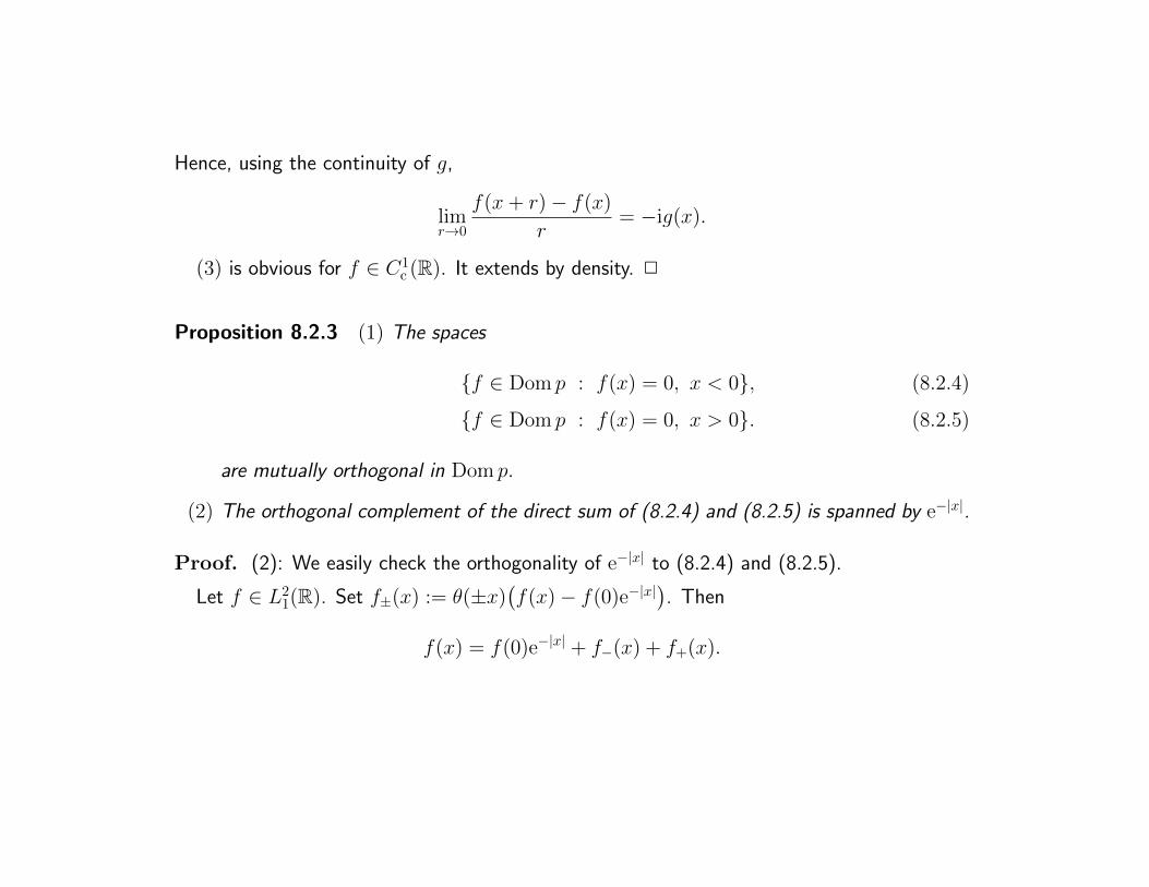
Hence, using the continuity of g,
limr→0
f(x+ r)− f(x)
r= −ig(x).
(3) is obvious for f ∈ C1c (R). It extends by density. 2
Proposition 8.2.3 (1) The spaces
f ∈ Dom p : f(x) = 0, x < 0, (8.2.4)
f ∈ Dom p : f(x) = 0, x > 0. (8.2.5)
are mutually orthogonal in Dom p.
(2) The orthogonal complement of the direct sum of (8.2.4) and (8.2.5) is spanned by e−|x|.
Proof. (2): We easily check the orthogonality of e−|x| to (8.2.4) and (8.2.5).
Let f ∈ L21(R). Set f±(x) := θ(±x)
(f(x)− f(0)e−|x|
). Then
f(x) = f(0)e−|x| + f−(x) + f+(x).

2
8.3 Momentum on the half-line
Consider the Hilbert space L2([0,∞[).
Define the semigroups
U←(t)f(x) := f(x+ t), t ≥ 0.
U→(t)f(x) :=
f(x− t), x ≥ t ≥ 0.
0, t > x,
Define pmax by
pmaxf(x) :=1
i∂xf(x), f ∈ Dom pmax := 1l[0,∞[f : f ∈ Dom p. (8.3.6)
Note that the graph scalar product of pmax is
(f |g)pmax=
∫ ∞0
(f(x)g(x) + f ′(x)g′(x)
)dx.

Define the operator pmin as the restriction of pmax to the domain
Dom pmin := f ∈ Dom p : f(x) = 0, x < 0.
(In the definitions of Dom pmax and Dom pmin we used concepts defined in the space L2(R),
however it is easy to see that both are subspaces of L2([0,∞[).)
Theorem 8.3.1 (1) We have U←(t) = eitpmax and U→(t) = e−itpmin.
(2) pmin ⊂ pmax, p∗min = pmax, p∗max = pmin; the operators pmin and −pmax are m-dissipative
(in particular, they are closed); the operator pmin is hermitian.
(3) Dom pmin is a subspace of Dom pmax of codimension 1 and its orthogonal complement is
spanned by 1l[0,∞[(x)e−x.
(4) C∞c ([0,∞[) is an essential domain of pmax and C∞c (]0,∞[) is an essential domain of pmin.
(5) sppmax = spppmax = Imz ≥ 0, sppmin = Imz ≤ 0, spppmin = ∅,
pmaxeizx = zeizx, eizx ∈ Dom pmax, Imz > 0; (8.3.7)

(6) The integral kernels of (z − pmax)−1 and (z − pmin)−1 are equal
Rmax(z, x, y) = iθ(y − x)eiz(x−y), Imz < 0.
Rmin(z, x, y) = −iθ(x− y)eiz(x−y), Imz > 0.
8.4 Momentum on an interval I
Consider the Hilbert space L2([−π, π]).
Define pmax as an operator with domain
Dom pmax =:= 1l[−π,π]f : f ∈ Dom p
and
pmaxf(x) :=1
i∂xf(x), f ∈ Dom pmax. (8.4.8)

Note that the graph scalar product for pmax is
(f |g)pmax=
∫ π
−π
(f(x)g(x) + f ′(x)g′(x)
)dx, f, g ∈ Dom pmax.
Define the operator pmin as the restriction of pmax to the domain
Dom pmin := f ∈ Dom p : f(x) = 0, x 6∈]− π, π[.
Theorem 8.4.1 (1) Neither pmax nor pmin generate a semigroup.
(2) pmin ⊂ pmax, p∗min = pmax, p∗max = pmin; the operators pmin and pmax are closed; the
operator pmin is hermitian.
(3) C∞([−π, π]) is an essential domain of pmax and C∞c (]− π, π[) is an essential domain of
pmin.
(4) sppmax = spppmax = C, sppmin = C, spppmin = ∅,
pmaxeizx = zeizx, z ∈ C, (8.4.9)

8.5 Momentum on an interval II
Let κ ∈ C. Define the family of groups on L2([−π, π]) by
Uκ(t)φ(x) = ei2πnκφ(x− t), −(2n− 1)π < x− t < −(2n+ 1)π, n ∈ Z.
Let the operator pκ be defined as the restriction of pmax to
Dom pκ = f ∈ Dom pmax : ei2πκf(−π) = f(π).
Theorem 8.5.1 (1) Uκ(t) = e−itpκ.
(2) ‖Uκ(t)‖ = e2πnImκ, 2π(n− 1) < t ≤ 2πn, n ∈ Z.
(3) The semigroup [0,∞[3 t 7→ Uκ(t) is of type (1, 0) for Imκ ≤ 0 and of type (e2πImκ, Imκ)
for Imκ ≥ 0.
(4) p∗κ = pκ, pκ = pκ+1; pmin ⊂ pκ ⊂ pmax. Operators pκ are closed. For κ ∈ R they
are self-adjoint.
(5) f ∈ C∞([−π, π]) : ei2πκf(−π) = f(π) is an essential domain of pκ.
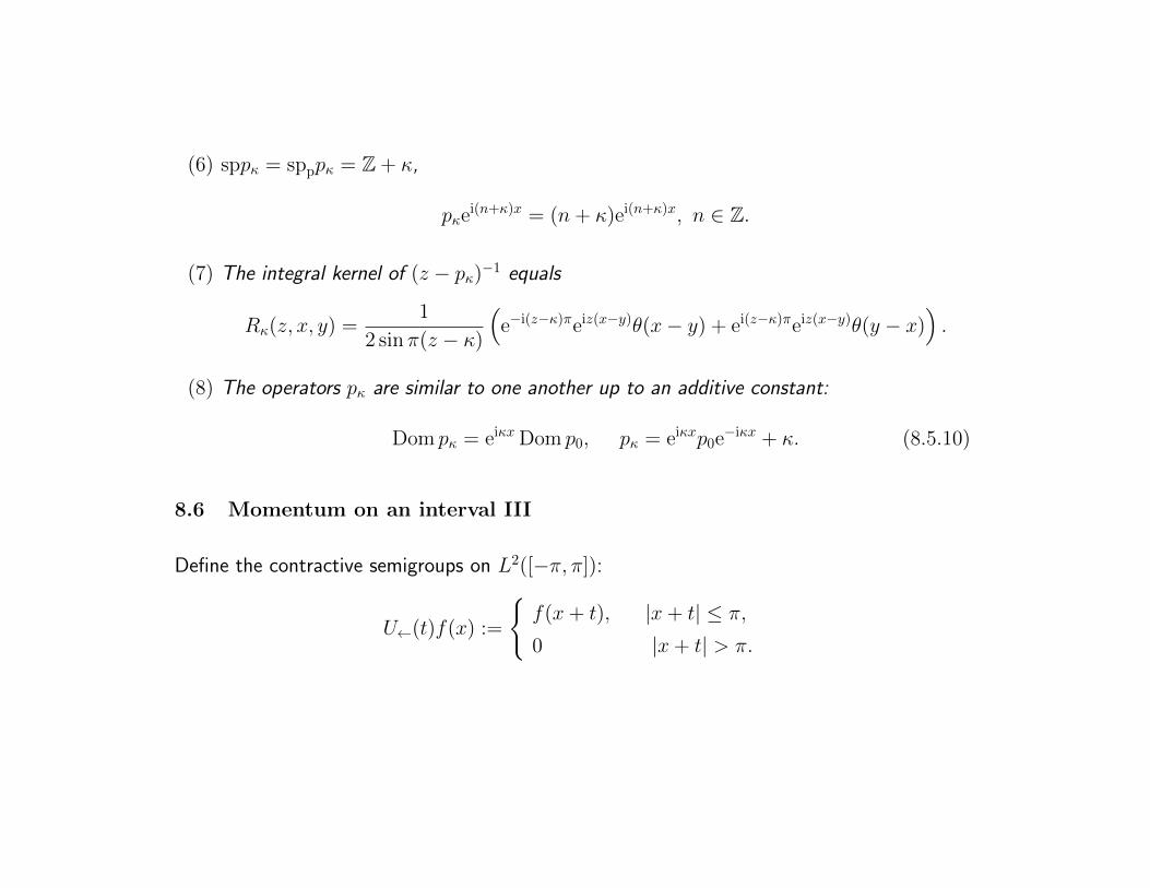
(6) sppκ = spppκ = Z + κ,
pκei(n+κ)x = (n+ κ)ei(n+κ)x, n ∈ Z.
(7) The integral kernel of (z − pκ)−1 equals
Rκ(z, x, y) =1
2 sinπ(z − κ)
(e−i(z−κ)πeiz(x−y)θ(x− y) + ei(z−κ)πeiz(x−y)θ(y − x)
).
(8) The operators pκ are similar to one another up to an additive constant:
Dom pκ = eiκx Dom p0, pκ = eiκxp0e−iκx + κ. (8.5.10)
8.6 Momentum on an interval III
Define the contractive semigroups on L2([−π, π]):
U←(t)f(x) :=
f(x+ t), |x+ t| ≤ π,
0 |x+ t| > π.

U→(t)f(x) :=
f(x− t), |x− t| ≤ π,
0 |x− t| > π..
Let the operator p±i∞ be defined as the restriction of pmax to
Dom p±i∞ = f ∈ Dom pmax : f(±π) = 0.
Theorem 8.6.1 (1) U←(t) = eitp+i∞ and U→(t) = e−itp−i∞.
(2) p∗±i∞ = p∓i∞; pmin ⊂ p±i∞ ⊂ pmax. Operators p±i∞ are closed.
(3) spp±i∞ = ∅.
(4) The integral kernel of (z − p±i∞)−1 equals
R±i∞(z, x, y) = ±ieiz(x−y±π)θ(±y ∓ x), z ∈ C.

Chapter 9
Laplacian
9.1 Sobolev spaces in one dimension
For α ∈ R let 〈p〉−αL2(R) be the scale of Hilbert spaces associated with the operator p. It is
called the scale of Sobolev spaces. We will focus in the case α ∈ N.
Theorem 9.1.1 (1)
〈p〉−nL2(R) = f ∈ L2(R) : f (n) ∈ L2(R).
181

(2) 〈p〉−nL2(R) ⊂ Cn−1(R) and 〈p〉−nL2(R) 3 f 7→ f (j)(x) for j = 0, . . . , n − 1 are
continuous functionals depending continuously on x ∈ R.
Proof. We use induction. The step n = 1 was proven before.
Suppose that we know that 〈p〉−nL2(R) ⊂ Cn(R). Let f ∈ 〈p〉−(n+1)L2(R). Then (i−p)f =
g ∈ 〈p〉−nL2(R). Clearly, 〈p〉−n−1L2(R) ⊂ 〈p〉−nL2(R), hence f ∈ Cn−1(R). Likewise,
g ∈ Cn−1(R), by the induction assumption. Now pf = −g + if ∈ Cn−1(R). Hence, by Prop.
8.2.2 (2) f ∈ Cn(R). 2
9.2 Laplacian on the line
Define the form d by
d(f, g) :=
∫f ′(x)g′(x)dx, f, g ∈ Dom d := 〈p〉−1L2(R).

The operator p2 on L2(R) will be denoted −∆. Thus
−∆f(x) = −∂2xf(x), f ∈ Dom(−∆) = 〈p〉−2L2(R).
Theorem 9.2.1 (1) −∆ is a positive self-adjoint operator.
(2) spp(−∆) = ∅.
(3) sp(−∆) = [0,∞[.
(4) The integral kernel of (k2 −∆)−1, for Rek > 0, is
R(k, x, y) =1
2ke−k|x−y|.
(5) The integral kernel of et∆ is
K(t, x, y) = (4πt)−12 e−
(x−y)2
4t .
(6) The form d is closed and associated with the operator −∆.

(7) f ∈ C2(R) ∩ L2(R) : f ′, f ′′ ∈ L2(R) is contained in Dom(−∆) and on this set
−∆f(x) = −∂2xf(x).
(8) C∞c (R) is an essential domain of −∆.
Proof. (4) Let Rek > 0. Then
(ik − p)−1(x, y) = −iθ(x− y)e−k|x−y|, (−ik − p)−1(x, y) = iθ(y − x)e−k|x−y|.
Now(k2 −∆)−1 = (ik − p)−1(−ik − p)−1
= (−2ik)−1((ik − p)−1 − (−ik − p)−1
).
(9.2.1)
The integral kernel of (9.2.1) equals (2k)−1e−k|x−y|.
(5) We have
et∆ = (2πi)−1
∫γ
(z −∆)−1etzdz,

where γ is a contour of the form e−iα]0,∞[∪eiα[0,∞[ bypassing 0, where π/2 < α < π. Hence
et∆(x, y) = (2πi)−1
∫γ
e−k|x−y|+tk2
dk
where γ is a contour of the form e−iα/2[0,∞[∪eiα/2[0,∞[. We put k = iu and obtain
et∆(x, y) = (2πi)−1
∫ ∞−∞
e−iu|x−y|−tu2
idu
2
9.3 Laplacian on the halfline I
Consider the space L2([0,∞[). Define −∆max by
−∆maxf = −∂2xf, f ∈ Dom
(−∆max
):= 1l[0,∞[f : f ∈ 〈p〉−2L2(R).
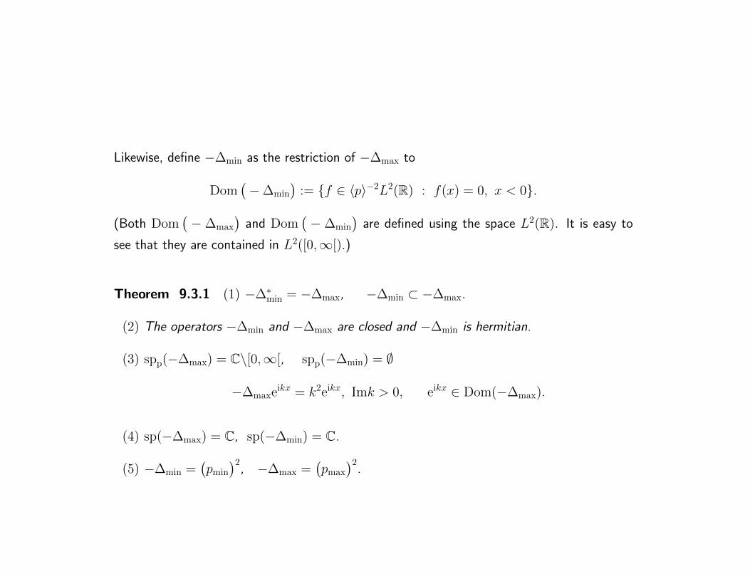
Likewise, define −∆min as the restriction of −∆max to
Dom(−∆min
):= f ∈ 〈p〉−2L2(R) : f(x) = 0, x < 0.
(Both Dom(− ∆max
)and Dom
(− ∆min
)are defined using the space L2(R). It is easy to
see that they are contained in L2([0,∞[).)
Theorem 9.3.1 (1) −∆∗min = −∆max, −∆min ⊂ −∆max.
(2) The operators −∆min and −∆max are closed and −∆min is hermitian.
(3) spp(−∆max) = C\[0,∞[, spp(−∆min) = ∅
−∆maxeikx = k2eikx, Imk > 0, eikx ∈ Dom(−∆max).
(4) sp(−∆max) = C, sp(−∆min) = C.
(5) −∆min =(pmin
)2, −∆max =
(pmax
)2.

9.4 Laplacian on the halfline II
Let µ ∈ C ∪ ∞. Let −∆µ be the restriction of −∆max to
Dom(−∆µ) = f ∈ Dom(−∆max) : µf(0) = f ′(0). (9.4.2)
(If µ =∞, these are the Dirichlet boundary conditions, that means f(0) = 0, if µ = 0, these
are the Neumann boundary conditions, that means f ′(0) = 0).
Define also the form dµ as follows. If µ ∈ R, then
dµ(f, g) := µf(0)g(0) +
∫f ′(x)g′(x)dx, f, g ∈ Dom dµ := Dom pmax.
For µ =∞,
d∞(f, g) :=
∫f ′(x)g′(x)dx, f, g ∈ Dom d∞ := Dom pmin.
Theorem 9.4.1 (1) −∆min ⊂ −∆µ ⊂ −∆max.
(2) −∆∗µ = −∆µ.
(3) The operator −∆µ is a generator of a group. For µ ∈ R ∪ ∞ it is self-adjoint.

(4) spp(−∆µ) =
−µ2, Reµ < 0;
∅, otherwise;
−∆µeµx = −µ2eµx, Reµ < 0, eµx ∈ Dom(−∆µ).
(5) sp(−∆µ) =
−µ2 ∪ [0,∞[, Reµ < 0,
[0,∞[, otherwise.
(6) −∆0 = p∗maxpmax, −∆∞ = p∗minpmin.
(7) The forms dµ are closed and associated with the operator −∆µ.
(8) Let Rek > 0. The integral kernel of (k2 −∆µ)−1 is equal
Rµ(k, x, y) =1
2ke−k|x−y| +
1
2k
(k − µ)
(k + µ)e−k(x+y),
in particular, for the Dirichlet boundary conditions,
R∞(z, x, y) =1
2ke−k|x−y| − 1
2ke−k(x+y),

and for the Neumann boundary conditions
R0(k, x, y) =1
2ke−k|x−y| +
1
2ke−k(x+y).
(9) The semigroups et∆µ have the integral kernel
Kµ(t, x, y) = (4πt)−12 e−
(x−y)2
4t + (2π)−1
∫ ∞−∞
iu− µiu+ µ
e−iu(x+y)−tu2
du,
In particular, in the Dirichlet case
K∞(t, x, y) = (4πt)−12 e−
(x−y)2
4t − (4πt)−12 e−
(x+y)2
4t ,
and in the Neumann case
K0(t, x, y) = (4πt)−12 e−
(x−y)2
4t + (4πt)−12 e−
(x+y)2
4t .
The group eit∆µ for µ ∈ R∪∞ describes a quantum particle with a potential well or bump
at the end of the halfline.
The semigroup et∆µ for µ ∈ R describes the diffusion with a sink or source at the end of the
halfline. Note that et∆µ preserves the pointwise positivity. If pt = et∆µp0, 0 < a < b, then
∂t
∫ b
a
pt(x)dx = p′(b)− p′(a).
∂t
∫ a
0
pt(x)dx = p′(a)− µp(0).
Thus at 0 there is a sink of p with the rate µ.
9.5 Neumann Laplacian on a halfline with the delta potential
On L2([0,∞[) we define the cosine transform
UNf(k) := π−1/2
∫ ∞0
cos kxf(x)dx, k ≥ 0.
Note that UN is unitary and U 2N = 1.
Let ∆N be the Laplacian on L2([0,∞[) with the Neumann boundary condition. Clearly,
−UN∆NU∗N = k2.

Let |δ)(δ| be the quadratic form given by
(f1|δ)(δ|f2) = f1(0)f2(0),
Note that it can be formally written as∫ ∞0
f(x)δ(x)g(x)dx,
and thus is interpreted as a “potential”.
Let (1| denote the functional on L2([0,∞[) given by
(1|g) =
∫ ∞0
g(k)dk.
Using δ(x) = π−1∫∞
0 cos kxdx we deduce that
UN|δ)(δ|U ∗N = π−1|1)(1|.
Then
UN (−∆N + λ|δ)(δ|)U ∗N = k2 + λπ−1|1)(1|

is an example of an Aronszajn-Donoghue Hamiltonian of type IIb, because∫ ∞0
1dk =∞,∫ ∞
0
1
1 + k2dk <∞,
∫ ∞0
1
k2dk =∞.
9.6 Dirichlet Laplacian on a halfline with the δ′ potential
On L2([0,∞[) we define the sine transform
UDf(k) := π−1/2
∫ ∞0
sin kxf(x)dx, k ≥ 0.
Note that UD is unitary and U 2D = 1
Let ∆D be the Laplacian on L2([0,∞[) with the Dirichlet boundary condition. Clearly,
−UD∆DU∗D = k2.
Using −δ′(x) = π−1∫∞
0 sin kxdx we deduce that
UD|δ′)(δ′|U ∗D = π−1|k)(k|.

Here |δ′)(δ′| is the quadratic form given by
(f1|δ′)(δ′|f2) = f ′1(0)f ′2(0),
and (k| is the functional on L2([0,∞[) given by
(k|g) =
∫ ∞0
kg(k)dk.
Thus
UD (−∆D + λ|δ′)(δ′|)U ∗ = k2 + λπ−1|k)(k|
is an example of an Aronszajn-Donoghue Hamiltonian of type IIIa, because∫ ∞0
k2
1 + k2dk =∞,
∫ ∞0
k2
(1 + k2)2dk <∞,
∫ ∞0
k2
(1 + k2)k2dk <∞.
9.7 Laplacian on L2(Rd) with the delta potential
On L2(Rd) we consider the unitary operator U = (2π)d/2F , where F is the Fourier transfor-
mation. Note that U is unitary.
Let ∆ be the usual Laplacian. Clearly,
−U∆U ∗ = k2.
Let |δ)(δ| be the quadratic form given by
(f1|δ)(δ|f2) = f1(0)f2(0).
Note that again it can be also written as∫f(x)δ(x)g(x)dx,

and thus is interpreted as a “potential”. Let (1| denote the functional on L2(Rd) given by
(1|g) =
∫g(k)dk.
Using δ(x) = (2π)−d∫
eikxdx we deduce that
U |δ)(δ|U ∗ = (2π)−d|1)(1|.
Consider
U (−∆ + λ|δ)(δ|)U ∗ = k2 + λ(2π)−d|1)(1|
as an example of an Aronszajn-Donoghue Hamiltonian. We compute:∫ddk
1 + k2<∞ ⇔ d = 1,∫
ddk
(1 + k2)2<∞ ⇔ d = 1, 2, 3,∫
ddk
k2(1 + k2)<∞ ⇔ d = 3.

Thus
(1) for d = 1 it is of type IIb, so it can be defined in the form sense using the parameter λ
(as we have already seen),
(2) for d = 2 it is of type IIIb. It can be renormalized.
(3) for d=3 it is of type IIIa. It can be renormalized.
(4) for d ≥ 4 there is no nontrivial renormalization procedure.
Consider dimension d = 2. Let us compute the resolvent for z = −p2. We have
g(−p2) = γ−1 + (p2 − 1)(1|(H0 + p2)−1(H0 + 1)−1|1)
= γ−1 + (p2 − 1)
∫d3k
(k2 + p2)(k2 + 1)= γ−1 + π ln p2.
Using that the Fourier transform of k 7→ 1k2+p2 equals x 7→ 2πK0(p|x|), where K0 is the 0th
MacDonald function, we obtain the following expression for the integral kernel of (p2 +H)−1:
2πK0(p|x− y|) +K0(p|x|)K0(p|y|)γ−1 + π ln p2
. (9.7.3)

In the physics literature one usually introduces the parameter a = eγ−1/2π called the scattering
length. There is a bound state K0(|x|/a) with eigenvalue −a−2.
Note that
f ∈ (1−∆)−1L2(R2) : f(0) = 0 (9.7.4)
is a closed subspace of (1−∆)−1L2(R2). The domain of H is spanned by (9.7.4) and
(−a−2 −∆)−1|1), (9.7.5)
which is in L2(R2)\(1−∆)−1L2(R2). In the position representation (9.7.5) is x 7→ 2πK0(|x|/a)
Around r ∼ 0 we have the asymptotics K0(r) ' − log(r/2)− γ. Therefore, the domain of H
contains functions that behave at zero as C(
log(|x|/2a) + γ).
Consider dimension d = 3. Let us compute the resolvent for z = −p2. We have
g(−p2) = γ0 + p2(1|(H0 + p2)−1H−10 |1)
= γ0 + p2
∫d3k
(k2 + p2)k2= γ0 + p4π2

Using that the Fourier transform of k 7→ 1k2+p2 equals x 7→ 2π2 ep|x|
|x| , we obtain the following
expression for the integral kernel of (p2 +H)−1:
2π2 e−p|x−y|
|x− y|+
πe−p|x|e−p|y|
2(γ0 + 4π2p)|x||y|. (9.7.6)
In the physics literature one usually introduces the parameter a = −(4πγ0)−1 called the scat-
tering length.
f ∈ (1−∆)−1L2(R3) : f(0) = 0 (9.7.7)
is a closed subspace of (1−∆)−1L2(R3). The domain of H is spanned by (9.7.7)
(aeiπ/4 − i)(i−∆)−1|1) + (ae−iπ/4 + i)(−i−∆)−1|1) (9.7.8)
In the position representation (±i − ∆)−1|1) equals x 7→ 2π2 exp(e±iπ/4|x|)|x| . Therefore, the
Hamiltonian with the scattering length a has the domain whose elements around zero behave
as C(1− a/|x|).
For a > 0 there is a bound state e−|x|/a
|x| with eigenvalue −a−2. To get the domain, instead
of (9.7.8), we can adjoin this bound state to (9.7.7).
Note that the Hamiltonian is increasing wrt γ0 ∈] − ∞,∞]. It is also increasing wrt a
separately on [−∞, 0] and ]0,∞]. At 0 the monotonicity is lost. a = 0 corresponds to the
usual Laplacian.
The following theorem summarizes a part of the above results.
Theorem 9.7.1 Consider −∆ on C∞c (Rd\0)
(1) It has the defficiency index (2, 2) for d = 1.
(2) It has the defficiency index (1, 1) for d = 2, 3.
(3) It is essentially self-adjoint for d ≥ 4.
(4) For d = 1 its Friedrichs extension is −∆D and its Krein extension is −∆.
(5) For d = 2 its Friedrichs and Krein extension is −∆.
(6) For d = 3 its Friedrichs extension is −∆ an its Krein extension corresponds to a =∞.

Let us sketch an alternative approach. The Laplacian in d dimensions written in spherical
coordinates equals
∆ = ∂2r +
d− 1
r∂r +
∆LB
r2,
where ∆LB is the Laplace-Beltrami operator on the sphere. For d ≥ 2, the eigenvalues of ∆LB
are −l(l + d − 2), for l = 0, 1, . . . . For d = 1 instead of the Laplace-Beltrami operator we
consider the parity operator with the eigenvalues ±1. We will write l = 0 for parity +1 and
l = 1 for parity −1. Hence the radial part of the operator is
∂2r +
d− 1
r∂r −
l(l + d− 2)
r2.
The indicial equation of this operator reads
λ(λ+ d− 2)− l(l + d− 2) = 0.
It has the solutions λ = l and λ = 2− l − d.
For l ≥ 2 only the solutions behaving as rl around zero are locally square integrable, the
solutions behaving as r2−1−d have to be discarded. For l = 0, 1 we have the following possible

square integrable behaviors around zero:
l = 0 l = 1 l ≥ 2
d = 1 r0, r1 r0, r1 −−d = 2 r0, r0 ln r r1 rl
d = 3 r0, r−1 r1 rl
d ≥ 4 r0 r1 rl
In dimension d = 1 in both parity sectors we have non-uniqueness of boundary conditions.
In dimensions d = 2, 3 this non-uniqueness appears only in the spherically symmetric sector.
There is no nonuniqueness in higher dimensions.

9.8 Approximating delta potentials by separable potentials
Set 1Λ(k) := 1l[0,Λ](|k|). The Laplacian with a delta potential can be conveniently approximated
by a separable potential
−∆ +λ
(2π)d|1Λ)(1Λ|. (9.8.9)
In dimension d = 1 and d = 2 (9.8.9) has a (single) negative bound state iff λ < 0.
Clearly, in dimension d = 1 (9.8.9) converges to −∆ + λδ in the norm resolvent sense for
all λ ∈ R.
It is easy to check that
−∆−(γ−1 + π log(1 + Λ2)
)−1|1Λ)(1Λ| (9.8.10)
converges to −∆(γ−1) for all γ−1 ∈ R.
In dimension d = 3 (9.8.9) has a (single) negative bound state for all λ(2π)3 < −(Λ4π)−1. It
is easy to check that
−∆−(γ0 + 4πΛ
)−1|1Λ)(1Λ| (9.8.11)

converges to −∆(γ0) for all γ0 ∈ R.


Chapter 10
Orthogonal polynomials
First we discuss some basic general facts about orthogonal polynomials. Then we will classify
the so called classical orthogonal polynomials, that is orthogonal polynomials that are eigefunc-
tions of a certain second order differential operator. We will show that all classical orthogonal
polynomials essentially fall into one of the following 3 classes:
205

(1) Hermite polynomials Hn(x) = (−1)n
n! ex2
∂xe−x2
, which form an orthogonal basis in L2(R, e−x2
)
and satisfy
(∂2x − 2x∂x + 2n)Hn(x) = 0.
(2) Laguerre polynomials Lαn(x) = 1n!e
x∂nxe−xxn+α , which form an orthogonal basis in
L2(]0,∞[, e−xxα) for α > −1 and satisfy
(x∂2x + (α + 1− x)∂x + n)Lαn(x) = 0.
(3) Jacobi polynomials P α,βn (x) = (−1)n
2nn! (1 − x)−α(1 + x)−β∂nx(1 − x)α+n(1 + x)β+n, which
form an orthogonal basis in L2(]− 1, 1[, (1− x)α(1 + x)β) for α, β > −1 and satisfy
(1− x2)∂2x + (β − α− (α + β + 2)x)∂x + n(n+ α + β + 1)P α,β
n (x) = 0.
An important role in the proof is played by unbounded operators. More precisely, we use the
fact that eigenvectors of hermitian operators with distinct eigenvalues are orthogonal.

Note that the proof is quite elementary – it has been routinely used in courses for physics
students of 2nd year of University of Warsaw. In particular, one does not need to introduce
the concept of a self-adjoint or essentially self-adjoint operator: one can limit oneself to the
concept of a hermitian operator, which is much less technical and acceptable for students
without sophisticated mathematical training.
10.1 Orthogonal polynomials
Let −∞ ≤ a < b ≤ ∞. Let ρ > 0 be a fixed positive integrable function on ]a, b[ called a
weight. Let x denote the generic variable in R.
We will denote by Pol the space of complex polynomials of the real variable. We assume
that ∫ b
a
|x|nρ(x)dx <∞, n = 0, 1, . . . . (10.1.1)
Then Pol is contained in L2([a, b], ρ).
The monomials 1, x, x2, . . . form a linearly independent sequence in L2([a, b], ρ). Applying

the Gram-Schmidt orthogonalization to this sequence we obtain the orthogonal polynomials
P0, P1, P2, . . . . Note that degPn = n. There exist a simple criterion that allows us to check
whether this is an orthogonal basis.
Theorem 10.1.1 Suppose that there exists ε > 0 such that∫ b
a
eε|x|ρ(x)dx <∞.
Then Pol is dense in L2([a, b], ρ). Therefore, P0, P1, . . . form an orthogonal basis of L2([a, b], ρ).
Proof. Let h ∈ L2([a, b], ρ). Then for |Imz| ≤ ε2∫ b
a
|ρ(x)h(x)eixz|dx ≤(∫ b
a
ρ(x)eε|x|dx
) 12(∫ b
a
ρ(x)|h(x)|2dx) 1
2
<∞.
Hence, for |Imz| ≤ ε2 we can define
F (z) :=
∫ b
a
ρ(x)e−izxh(x)dx.
F is analytic in the strip z ∈ C : |Imz| < ε2. Let (xn|h) = 0, n = 0, 1, . . . . Then
dn
dznF (z)
∣∣∣z=0
= (−i)n∫ b
a
xnρ(x)h(x)dx = (−i)n(xn|h) = 0.
But an analytic function vanishing with all derivatves at one point vanishes in its whole (con-
nected) domain. Hence F = 0 in the whole strip, and in particular on the real line. Hence
h = 0. Applying the inverse Fourier transformation we obtain h = 0.
Therefore, there are no nonzero vectors orthogonal to Pol. 2
10.2 Reminder about hermitian operators
In this chapter we will need some minimal knowledge about hermitian operators. In order to
make it essentially self-contained, we recall that an operator A is hermitian if
(w|Av) = (Aw|v), v, w ∈ DomA.
Theorem 10.2.1 Let A be a hermitian operator.

(1) If v ∈ DomA is its eigenvector with eigenvalue λ, that is Av = λv, then λ ∈ R.
(2) If λ1 6= λ2 are its eigenvalues with eigenvectors v1 and v2, then v1 is orthogonal to v2.
Proof. To prove (1), we note that
λ(v|v) = (v|Av) = (Av|v) = λ(v|v).
then we divide by (v|v) 6= 0.
Proof of (2):
(λ1 − λ2)(v1|v2) = (Av1|v2)− (v1|Av2) = (v1|Av2)− (v1|Av2) = 0.
2
Remark 10.2.2 In finite dimension we can always find an orthonormal basis consisting of
eigenvectors of a hermitian operators. In infinite dimension this is not always the case. If it
happens then the operator is essentially self-adjoint.

10.3 2nd order differential operators
A general 2nd order differential operator without a 0th order term can be written as
C := σ(x)∂2x + τ(x)∂x, (10.3.2)
for some functions σ(x) and τ(x).
It is often convenient to rewrite C in a different form. Let ρ(x) satisfy
σ(x)ρ′(x) = (τ(x)− σ′(x))ρ(x). (10.3.3)
We have then
C = ρ(x)−1∂xρ(x)σ(x)∂x. (10.3.4)
The form (10.3.4) of the operator C is convenient for the study of its hermiticity.
To simplify the exposition, in the remaining part of this subsection we will assume that a = 0
and b = ∞, which will illustrate the two possible types of endpoints. The generalization to
arbitrary a < b will be obvious.

Theorem 10.3.1 Assume (10.1.1). Suppose also that
(1) ρ and σ are real differentiable functions on ]0,∞[ and ρ > 0;
(2) at the boundaries of the interval we have
σ(0)ρ(0) = 0,
limx→∞
σ(x)ρ(x)|x|n = 0, n = 0, 1, 2, . . . .
Then C as an operator on L2([0,∞[, ρ) with domain Pol is hermitian.
Proof.
(g|Cf) =
∫ ∞0
ρ(x)g(x)ρ(x)−1∂xσ(x)ρ(x)∂xf(x)dx
= limR→∞
∫ R
0
g(x)∂xσ(x)ρ(x)∂xf(x)dx
= limR→∞
g(x)ρ(x)σ(x)f ′(x)∣∣∣R0− lim
R→∞
∫ R
0
(∂xg(x))σ(x)ρ(x)∂xf(x)dx
= − limR→∞
g′(x)ρ(x)σ(x)f(x)∣∣∣R0
+ limR→∞
∫ R
0
(∂xρ(x)σ(x)∂xg(x))f(x)dx
=
∫ ∞0
ρ(x)(ρ(x)−1∂xσ(x)ρ(x)∂xg(x))f(x)dx = (Cg|f).
2
Self-adjoint operators of the form (10.3.4) are often called Sturm-Liouville operators.

10.4 Hypergeometric type operators
We are looking for 2nd order differential operators whose eigenfunctions are polynomials. This
restricts severely the form of such operators.
Theorem 10.4.1 Let
C := σ(z)∂2z + τ(z)∂z + η(z) (10.4.5)
Suppose there exist polynomials P0, P1, P2 of degree 0, 1, 2 respectively, satisfying
CPn = λnPn.
Then
(1) σ(z) is a polynomial of degree ≤ 2,
(2) τ(z) is a polynomial of degree ≤ 1,
(3) η(z) is a polynomial of degree ≤ 0 (in other words, it is a number).
Proof. CP0 = η(z)P0, hence deg η = 0.

CP1 = τ(z)P ′1 + ηP1, hence deg τ ≤ 1.
CP2 = σ(z)P ′′2 + τ(z)P ′2(z) + ηP2, hence deg σ ≤ 2. 2
Clearly, the number η can be included in the eigenvalue. Therefore, it is enough to consider
operators of the form
C := σ(z)∂2z + τ(z)∂z, (10.4.6)
where deg σ ≤ 2 and deg τ ≤ 1. We will show that for a large class of (10.4.6) there exists
for every n ∈ N a polynomial Pn of degree n that is an eigenfunction of (10.4.6).
The eigenvalue equation of (10.4.6), that is equations of the form(σ(z)∂2
z + τ(z)∂z + λ)f(z) = 0,
will be called hypergeometric type equations. Solutions of these equations will be called hyper-
geometric type functions. Polynomial solutions will be called hypergeometric type polynomials.

10.5 Generalized Rodrigues formula
Some of the properties of hypergeometric type polynomials can be introduced in a unified way.
Let ρ satisfy
σ(z)∂zρ(z) = (τ(z)− σ′(z)) ρ(z). (10.5.7)
Note that ρ can be expressed by elementary functions.
Let us fix σ. We will however make explicit the dependence on ρ. The operator C(ρ) can
be written as
C(ρ) = ρ−1(z)∂zσ(z)ρ(z)∂z (10.5.8)
= ∂zρ−1(z)σ(z)∂zρ(z)− τ ′ + σ′′. (10.5.9)
The following is a generalization of the Rodrigues formula, originally given in the case of

Legendre polynomials:
Pn(ρ; z) :=1
n!ρ−1(z)∂nz σ
n(z)ρ(z) (10.5.10)
=1
2πiρ−1(z)
∫[0+]
σn(z + t)ρ(z + t)t−n−1dt. (10.5.11)
Theorem 10.5.1 Pn is a polynomial, typically of degree n, more precisely its degree is given
as follows:
(1) If σ′′ = τ ′ = 0, then degPn = 0.
(2) If σ′′ 6= 0 and −2τ ′
σ′′ + 1 = m is a positive integer, then
degPn =
n, n = 0, 1, . . . ,m;
n−m− 1, n = m+ 1,m+ 2, . . . .
(3) Otherwise, degPn = n.

We have (σ(z)∂2
z + τ(z)∂z)Pn(ρ; z) = (nτ ′ + n(n− 1)
σ′′
2)Pn(ρ; z), (10.5.12)
(σ(z)∂z + τ(z)− σ′(z))Pn(ρ; z) = (n+ 1)Pn+1(ρσ−1; z), (10.5.13)
∂zPn(ρ; z) =
(τ ′ + (n− 1)
σ′′
2
)Pn−1(ρσ; z), (10.5.14)
ρ(z + tσ(z))
ρ(z)=
∞∑n=0
tnPn(ρσn; z). (10.5.15)
Proof. Introduce the following creation and annihilation operators:
A+(ρ) := σ(z)∂z + τ(z) = ρ−1(z)∂zρ(z)σ(z),
A− := ∂z.

Note that
C(ρ) = A+(ρ)A−
= A−A+(ρσ−1)− τ ′ + σ′′.
Hence
C(ρ)A+(ρ) = A+(ρ)A−A+(ρ)
= A+(ρ)(C(ρσ) + τ ′
).
Therefore, if C(ρσn)F0 = λ0F0, then
C(ρ) A+(ρ) · · ·A+(ρσn−1)F0
=(λ0 + nτ ′ + n(n− 1)
σ′′
2
)A+(ρ) · · ·A+(ρσ−1)F0.

Using
A+(ρ) = ρ−1(z)∂zρ(z)σ(z),
A+(ρσ) = ρ−1(z)σ−1(z)∂zρ(z)σ2(z),
· · · = · · ·
A+(ρσn−1) = ρ−1(z)σ−(n−1)∂zρ(z)σn(z),
we obtain
A+(ρ) · · ·A+(ρσn−1)F0 = ρ(z)−1∂nz ρ(z)σn(z)F0(z).
Take F0 = 1, for which λ0 = 0. We then obtain (10.5.12). 2

10.6 Classical orthogonal polynomials as eigenfunctions of a Sturm-Liouville
operator
We are looking for −∞ ≤ a < b ≤ ∞ and weights ]a, b[3 x 7→ ρ(x) with the following
properties: There exist polynomials P0, P1, . . . satisfying degPn = n which form an orthogonal
basis of L2(]a, b[, ρ) and are eigenfunctions of a certain 2nd order differential operator C :=
σ(x)∂2x + τ(x)∂x, that is, for some λn ∈ R(
σ(x)∂2x + τ(x)∂x + λn
)Pn(x) = 0. (10.6.16)
In particular, we want C to be hermitian on Pol.
We know that one has to satisfy the following conditions:
(1) For any n ∈ N ∫ b
a
ρ(x)|x|ndx <∞, (10.6.17)
which guarantees that Pol ⊂ L2(]a, b[, ρ).
(2) σ has to be a polynomial of degree at most 2 and τ a polynomial of degree at most 1.

(See Thm 10.4.1).
(3) The weight ρ has to solve
σ(x)ρ′(x) = (τ(x)− σ′(x))ρ(x), (10.6.18)
to be positive, σ has to be real. (See Thm 10.3.1 (1)).
(4) We have to check the boundary conditions
(i) If an endpoint, say, a is a finite number, we check whether ρ(a)σ(a) = 0.
(ii) If an endpoint is infinite, say a = −∞, then
limx→−∞
|x|nσ(x)ρ(x) = 0, n = 0, 1, 2, . . . .
(see Thm 10.3.1 (2).)
We will find all weighted spaces L2(]a, b[, ρ) satisfying the conditions (1)-(4). It will turn

out that in all cases the condition ∫ b
a
eε|x|ρ(x)dx <∞ (10.6.19)
for some ε > 0 will hold, which will guarantee that we obtain an orthogonal basis (see Thm
10.1.1).
We will simplify our answers to standard forms
(1) by changing the variable x 7→ αx+ β for α 6= 0;
(2) by dividing (both the differential equation and the weight) by a constant.
As a result, we will obtain all classical orthogonal polynomials.
10.7 Classical orthogonal polynomials for deg σ = 0
We can assume that σ(x) = 1.
If deg τ = 0, then
C = ∂2y + c∂y.

It is easy to discard this case.
Hence deg τ = 1. Thus
C = ∂2y + (ay + b)∂y.
Let us set x =√|a|2
(y + b
a
). We obtain
C = ∂2x + 2x∂x, a > 0; (10.7.20)
C = ∂2x − 2x∂x, a < 0. (10.7.21)
Thus ρ(x) = e±x2
.
σ(x)ρ(x) = e±x2
is never zero, hence the only possible interval is ]−∞,∞[.
If a > 0, we have ρ(x) = ex2
, which is impossible because of (4ii).
If a < 0, we have ρ(x) = e−x2
and the interval ] −∞,∞[ is admissible, and even satisfes
(10.6.19). We obtain Hermite polynomials

10.8 Classical orthogonal polynomials for deg σ = 1
We can assume that σ(y) = y.
If deg τ = 0, then
C = y∂2y + c∂y
Such a C always decreases the degree of a polynomial. Therefore, if P is a polynomial and
CP = λP , then λ = 0. Hence P (x) = x−c. Therefore, we do not obtain polynomials of all
degrees as eigenfunctions.
Thus deg τ = 1. Hence, for b 6= 0,
y∂2y + (a+ by)∂y. (10.8.22)
After rescaling, we obtain the operator:
C = −x∂2x + (−α− 1 + x)∂x.
We compute: ρ = xαe−x. ρ(x)σ(x) = xα+1e−x is zero only for x = 0 i α > −1. The

interval [−∞, 0] is eliminated by (4ii). The interval [0,∞] is admissible for α > −1, and even
it satisfies 10.6.19. We obtain Laguerre polynomials.
10.9 Classical orthogonal polynomials for deg σ = 2,
σ has a double root
We can assume that σ(x) = x2.
If τ(0) = 0, then
C = x2∂2x + cx∂x.
xn are eigenfunctions of this operator, but the weight ρ(x) = xc−2 is not good.
Let us assume now that τ(0) 6= 0. After rescaling we can suppose that
τ(x) = 1 + (γ + 2)x.
This gives ρ(x) = e−1xxγ. The only point where ρ(x)σ(x) = e−
1xxγ+2 can be zero is x = 0.
Hence the only possible intervals are ]−∞, 0[ and ]0,∞[. Both are eliminated by (4ii).

10.10 Classical orthogonal polynomials for deg σ = 2,
σ has two roots
If both roots are imaginary, it suffices to assume that σ(x) = 1 + x2. We can suppose that
τ(x) = a+ (b+ 2)x. Then ρ(x) = ea arctanx(1 + x2)b. σ(x)ρ(x) is nowhere zero and therefore
the only admissble interval is [−∞,∞]. This has to be rejected, because lim|x|→∞ ρ(x)|x|n(1+
x2) =∞ for large enough n.
Thus we can assume that the roots are real. It suffices to assume that σ(x) = 1− x2. Let
τ(x) = β − α− (α + β − 2)x,
which corresponds to the operator
(1− x2)∂2x + (β − α− (α + β − 2)x∂x,
We obtain ρ(x) = |1 − x|β|1 + x|α. (4ii) eliminates the intervals ] −∞,−1[ and ]1,∞[.
There remains only the interval [−1, 1], which satisfies (4i) for α, β > −1. We obtain Jacobi
polynomials.

Chapter 11
Homogeneous Schrodinger operators
This chapter is partly based on the joint work with V.Georgescu and L.Bruneau. Some of the
results (in particular (11.3.6)) were obtained independently by Pankrashkin and Richard.
11.1 Modified Bessel equation
229
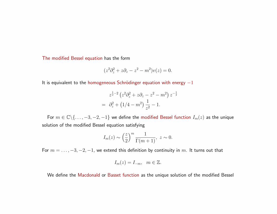
The modified Bessel equation has the form
(z2∂2z + z∂z − z2 −m2)v(z) = 0.
It is equivalent to the homogeneous Schrodinger equation with energy −1
z12−2(z2∂2
z + z∂z − z2 −m2)z−
12
= ∂2z +
(1/4−m2
) 1
z2− 1.
For m ∈ C\. . . ,−3,−2,−1 we define the modified Bessel function Im(z) as the unique
solution of the modified Bessel equation satisfying
Im(z) ∼(z
2
)m 1
Γ(m+ 1), z ∼ 0.
For m = . . . ,−3,−2,−1, we extend this definition by continuity in m. It turns out that
Im(z) = I−m, m ∈ Z.
We define the Macdonald or Basset function as the unique solution of the modified Bessel

equation satisfying, for | arg z| > π − ε,
lim|z|→∞
Km(z)e−z√π√
2z
= 1.
We have the relations
K−m(z) = Km(z) =π
2 sinπm(I−m(z)− Im(z)), (11.1.1)
Im(z) =1
iπ
(Km(e−iπz)− eiπmKm(z)
). (11.1.2)
As x→ 0, we have
Km(x) ∼
Re(Γ(m)
(2x
)m)if Rem = 0, m 6= 0;
− ln(x2
)− γ if m = 0,
Γ(m)2
(2x
)mif Rem > 0;
Γ(−m)2
(x2
)mif Rem < 0.
(11.1.3)

From a single solution we can generate a whole ladder of solutions:(1
z∂z
)nzmIm(z) = zm−nIm−n(z),(
1
z∂z
)nz−mIm(z) = z−m−nIm+n(z).
Analoguous identities hold for Km(z).
For m = ±12 (and hence for all m ∈ Z+ 1
2) the modified Bessel and the MacDonald functions
can be expressed in terms of elementary functions:
I 12(z) =
(2
πz
) 12
sinh z
I− 12(z) = =
(2
πz
) 12
cosh z,
K− 12(z) = K 1
2(z) =
( π2z
) 12
e−z.

11.2 Standard Bessel equation
Replacing z with ±iz in the modified Bessel equation leads to the standard Bessel equation:
(z2∂2z + z∂z + z2 −m2)v(z) = 0.
It is equivalent to the homogeneous Schrodinger equation with energy 1
z12−2(z2∂2
z + z∂z + z2 −m2)z−
12
= ∂2z +
(1/4−m2
) 1
z2+ 1.
For m ∈ C\. . . ,−3,−2,−1 we define the Bessel function Jm(z) as the unique solution
of the Bessel equation satisfying
Jm(z) ∼(z
2
)m 1
Γ(m+ 1), z ∼ 0.
For m = . . . ,−3,−2,−1, we extend this definition by continuity in m. It turns out that
Jm(z) = (−1)mJ−m, m ∈ Z.

It is simply related to the modified Bessel function:
Jm(z) = e±iπm2 Im(∓iz).
There are two Hankel functions. They can be defined as the unique functions satisfying the
following asymptotic formulas are true for −π + δ < arg z < 2π − δ, δ > 0:
limz→∞
H+m(z)(
2πz
) 12 eize−
imπ2 −
iπ4
= 1,
limz→∞
H−m(z)(2πz
) 12 e−ize
imπ2 + iπ
4
= 1.
Both are analytic continuations of the MacDonald function – one to the lower and the other
to the upper part of the complex plane:
H±m(z) =±2
iπe∓iπm2 Km(∓iz),
Km(z) = ± iπ
2e±imπH±(±iz).

Note the identitiesH±−m(z) = e±mπiH±m(z),
Jm(z) = 12 (H+
m(z) +H−m(z)) ,
J−m(z) = 12
(emπiH+
m(z) + e−mπiH−m(z)),
H±m(z) = ± ie∓mπiJm(z)−iJ−m(z)sinmπ ,
From a single solution we can generate a whole ladder of solutions:(1
z∂z
)nzmJm(z) = zm−nJm−n(z),(
−1
z∂z
)nz−mJm(z) = z−m−nJm+n(z).
Analogous identities hold for H±m(z).
For m = ±12 (and hence for all m ∈ Z+ 1
2) the modified Bessel and the MacDonald functions

can be expressed in terms of elementary functions:
J 12(z) = =
(2
πz
) 12
sin z,
J− 12(z) =
(2
πz
) 12
cos z,
H±12
(z) =
(2
πz
) 12
e±i(z−π2 ),
H±− 12
(z) =
(2
πz
) 12
e±iz
11.3 Homogeneous Schrodinger operators
Let Uτ be the group of dilations on L2[0,∞[, that is (Uτf)(x) = eτ/2f(eτx). We say that an
operator A is homogeneous of degree ν if UτAU−1τ = e−ντA.
Let D := 12(xp+ px) denote the generator of dilations, so that Uτ = e−iτD.
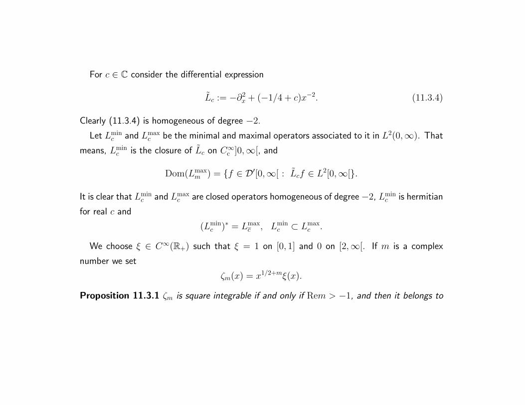
For c ∈ C consider the differential expression
Lc := −∂2x + (−1/4 + c)x−2. (11.3.4)
Clearly (11.3.4) is homogeneous of degree −2.
Let Lminc and Lmax
c be the minimal and maximal operators associated to it in L2(0,∞). That
means, Lminc is the closure of Lc on C∞c ]0,∞[, and
Dom(Lmaxm ) = f ∈ D′[0,∞[ : Lcf ∈ L2[0,∞[.
It is clear that Lminc and Lmax
c are closed operators homogeneous of degree −2, Lminc is hermitian
for real c and
(Lminc )∗ = Lmax
c , Lminc ⊂ Lmax
c .
We choose ξ ∈ C∞(R+) such that ξ = 1 on [0, 1] and 0 on [2,∞[. If m is a complex
number we set
ζm(x) = x1/2+mξ(x).
Proposition 11.3.1 ζm is square integrable if and only if Rem > −1, and then it belongs to

DomLmaxm2 . For Rem > 1, ζm belongs also to DomLmin
m2 , otherwise it does not.
For Re(m) > −1, we define Hm to be the operator Lmaxm2 restricted to Dom(Lmin
m2 ) + Cζm.
We will see that the family of operators m 7→ Hm possesses very good properties. The main
tool in its investigation is its resolvent, which can be computed explicitly.
Theorem 11.3.2 (1) The operators Hm are homogeneous of degree −2
(2) Hm = Lminm2 = Lmax
m2 iff Rem > 1.
(3) For any Re(m) > −1 we have sp(Hm) = [0,∞[.
(4) Let λ ∈ C\[0,∞[. Set Rm(λ;x, y) to be the integral kernel of (λ − Hm)−1. Then for
Rek > 0 we have
Rm(−k2;x, y) =
√xyIm(kx)Km(ky) if x < y,√xyIm(ky)Km(kx) if x > y.
,
where Im is the modified Bessel function and Km is the MacDonald function.
(5) The resolvent (λ−Hm)−1 is an analytic function of m for Rem > −1. As Rem approaches
−1, its norm blows up.

(6) We have H∗m = Hm. In particular, Hm is self-adjoint and positive iff m is real.
In the following theorem we describe the self-adjoint extensions of Lminc for various real values
of c.
Theorem 11.3.3 (1) If 1 ≤ c, then Lminc = Lmax
c = Hm with m =√c is self-adjoint. In
particular, Hm is essentially self-adjoint on C∞c ]0,∞[.
(2) If 0 < c < 1, then a subspace of DomLmaxc complementary to DomLmin
c is spanned by
ζm and ζ−m with m =√c. Self-adjoint extensions are obtained by adjoining to DomLmin
c
cosαζm + sinαζ−m.
Among them we have Hm, which is the Friedrichs extension of Lminc , and H−m, which is
its Krein extension.
(3) A subspace of DomLmax0 complementary to DomLmin
0 is spanned by ζ0 and log xζ0.
Self-adjoint extensions are obtained by adjoining to DomLmin0
cosαζ0 + sinα log xζ0.

Among them there is H0, which is both a Friedrichs and Krein extension of Lmin0 .
(4) If c ≤ 0, then a subspace of DomLmaxc complementary to DomLmin
c is spanned by ζik
and ζ−ik with k =√−c. Self-adjoint extensions are obtained by adjoining to DomLmin
c
eiαζik + e−iαζ−ik.
H−ik and Hik are non-self-adjoint extensions of Lminc .
Theorem 11.3.4 (1) 0 ≤ m ≤ m′ ⇒ Hm ≤ Hm′.
(2) 0 ≤ m < 1⇒ H−m ≤ Hm.
(3) If 0 ≤ argm ≤ π/2, then Num(Hm) = z : 0 ≤ arg z ≤ 2 argm.
(4) If −π/2 ≤ argm ≤ 0, then Num(Hm) = z : 2 argm ≤ arg z ≤ 0.
(5) If π/2 < | argm| < π, then Num(Hm) = C.
In the following theorem we show how to compute various quantities closely related to the
operators Hm. We restrict ourselves to the case of real m.

Theorem 11.3.5 (1) For 0 < a < b <∞, the integral kernel of 1l[a,b](Hm) is
1l[a,b](Hm)(x, y) =
∫ √b√a
√xyJm(kx)Jm(ky)kdk,
where Jm is the Bessel function.
(2) Let Fm be the operator on L2[0,∞] given by
Fm : f(x) 7→∫ ∞
0
Jm(kx)√kxf(x)dx (11.3.5)
Up to an inessential factor, Fm is the so-called Hankel transformation. Fm is a unitary
involution on L2[0,∞] diagonalizing Hm, more precisely
FmHmF−1m = x2.
It satisfies FmeitD = e−itDFm for all t ∈ R.
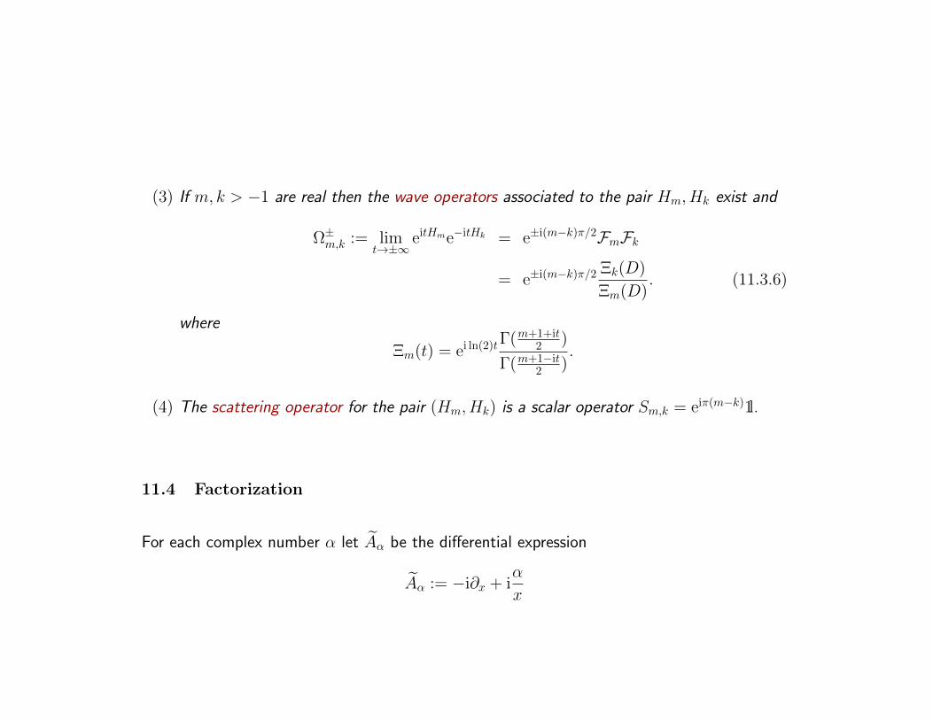
(3) If m, k > −1 are real then the wave operators associated to the pair Hm, Hk exist and
Ω±m,k := limt→±∞
eitHme−itHk = e±i(m−k)π/2FmFk
= e±i(m−k)π/2 Ξk(D)
Ξm(D). (11.3.6)
where
Ξm(t) = ei ln(2)tΓ(m+1+it2 )
Γ(m+1−it2 )
.
(4) The scattering operator for the pair (Hm, Hk) is a scalar operator Sm,k = eiπ(m−k)1l.
11.4 Factorization
For each complex number α let Aα be the differential expression
Aα := −i∂x + iα
x

acting on distributions on R+. Its restriction to C∞c ]0,∞[ is a closable operator in L2[0,∞[
whose closure will be denoted Aminα . This is the minimal operator associated to Aα. The
maximal operator Amaxα associated to Aα is defined as the restriction of Aα to Dom(Amax
α ) :=
f ∈ L2[0,∞[ : Aαf ∈ L2[0,∞[.The following properties of the operators Amin
α and Amaxα are easy to check:
(i) Aminα ⊂ Amax
α ,
(ii) (Aminα )∗ = Amax
−α and (Amaxα )∗ = Amin
−α ,
(iii) Aminα and Amax
α are homogeneous of degree −1.

Proposition 11.4.1 (1) We have Aminα = Amax
α if and only if |Reα| ≥ 1/2.
(2) Let Reα > −1/2. Then
(i) rs(Amaxα ) = C−.
(ii) The map α 7→ Amaxα is holomorphic in the region Reα > −1/2.
(iii) If Reα ≥ 0 then iAmaxα is the generator of a C0-semigroup of contractions
(1) Let Reα < 1/2. Then
(i) rs(Aminα ) = C+.
(ii) The map α 7→ Aminα is holomorphic in the region Reα < 1/2.
(iii) if Reα ≤ 0 the operator −iAminα is the generator of a C0-semigroup of contractions

m ≥ 1: Hm = A∗1/2+mA1/2+m = A∗1/2−mA1/2−m, H10 = Q(Hm),
Hm = Lminm2 = Lmax
m2 ;
0 < m < 1: Hm = A∗1/2+mA1/2+m =(Amin
1/2−m
)∗Amin
1/2−m H10 = Q(Hm),
Hm is the Friedrichs ext. of Lminm2 ;
m = 0: H0 = A∗1/2A1/2, H10 + Cζ0 dense in Q(H0),
H0 is the Friedrichs and Krein ext. of Lmin0 ;
−1 < m < 0: Hm =(Amax
1/2+m
)∗Amax
1/2+m, H10 + Cζm = Q(Hm),
Hm is the Krein ext. of Lminm2 .
In the region −1 < m < 1 (which is the most interesting one), it is quite remarkable that
for strictly positive m one can factorize Hm in two different ways, whereas for m ≤ 0 only one
factorization appears.
As an example, let us consider the case of the Laplacian −∂2x, i.e. m2 = 1/4. The operators

H1/2 and H−1/2 coincide with the Dirichlet and Neumann Laplacian respectively. One usually
factorizes them as H1/2 = P ∗minPmin and H−1/2 = P ∗maxPmax, where Pmin and Pmax denote the
usual momentum operator on the half-line with domain H10[0,∞[ and H1[0,∞[ respectively.
The above analysis says that, whereas for the Neumann Laplacian this is the only factorization
of the form S∗S with S homogeneous, in the case of the Dirichlet Laplacian one can also
factorize it in the rather unusual following way
H1/2 =(Pmin + ix−1
)∗ (Pmin + ix−1
).
11.5 Hm as a holomorphic family of closed operators
The definition (or actually a number of equivalent definitions) of a holomorphic family of
bounded operators is quite obvious and does not need to be recalled. In the case of unbounded
operators the situation is more subtle.
Suppose that Θ is an open subset of C, H is a Banach space, and Θ 3 z 7→ H(z) is a
function whose values are closed operators on H. We say that this is a holomorphic family

of closed operators if for each z0 ∈ Θ there exists a neighborhood Θ0 of z0, a Banach space
K and a holomorphic family of injective bounded operators Θ0 3 z 7→ A(z) ∈ B(K,H) such
that RanA(z) = D(H(z)) and
Θ0 3 z 7→ H(z)A(z) ∈ B(K,H)
is a holomorphic family of bounded operators.
We have the following practical criterion:
Theorem 11.5.1 Suppose that H(z)z∈Θ is a function whose values are closed operators
on H. Suppose in addition that for any z ∈ Θ the resolvent set of H(z) is nonempty.
Then z 7→ H(z) is a holomorphic family of closed operators if and only if for any z0 ∈ Θ
there exists λ ∈ C and a neighborhood Θ0 of z0 such that λ ∈ rs(H(z)) for z ∈ Θ0 and
z 7→ (H(z)− λ)−1 ∈ B(H) is holomorphic on Θ0.
The above theorem indicates that it is more difficult to study holomorphic families of closed
operators that for some values of the complex parameter have an empty resolvent set.

It is interesting to note that Ξm(D) is a unitary operator for all real values of m and
Ξ−1m (D)x−2Ξm(D) (11.5.7)
is a function with values in self-adjoint operators for all real m. Ξm(D) is bounded and
invertible also for all m such that Rem 6= −1,−2, . . . . Therefore, the formula (11.5.7) defines
an operator for all m | Rem 6= −1,−2, . . . ∪ R. Clearly, for Rem > −1, this operator
function coincides with the operator Hm studied in this paper. Its spectrum is always equal to
[0,∞[ and it is analytic in the interior of its domain.
One can then pose the following question: does this operator function exetnd to a holomor-
phic function of closed operators on the whole complex plane?

Bibliography
[Da] Davies, E. B.: One parameter semigroups, Academic Press 1980
[Ka] Kato, T.: Perturbation theory for linear operators, Springer 1966
[RS1] Reed, M., Simon, B.: Methods of Modern Mathematics, vol. 1, Academic Press 1972
[RS2] Reed, M., Simon, B.: Methods of Modern Mathematics, vol. 4, Academic Press 1978
249


![AdS-Phobiasp18.fuw.edu.pl/wp-content/uploads/participants-database/ads... · [See Irene’s talk] ... [Arkani-Hamed, Dubovski, Nicolis, Villadoro ’07] ADS-PHOBIA AND THE SM [Arnold,](https://img.pdfslide.net/doc/110x75/5c660b9109d3f2d12a8ba887/ads-see-irenes-talk-arkani-hamed-dubovski-nicolis-villadoro-07.jpg)