EUROPEAN COMMISSION

nuclear science and technology

Validation of Constraint-Based Assessment Methodology in Structural Integrity

(VOCALIST)

Editor: David Lidbury, Serco Assurance (UK)

Final report Part I (technical report)

Contract No: FIKS CT-2000-00090

Work performed as part of the European Atomic Energy Community's R&T specific programme Nuclear Energy, key action Nuclear Fission Safety, 1998-2002

Area: Operational Safety of Existing Installations

Directorate-General for Research 2006 Euratom

II

Project coordinator Serco Assurance Partners Serco Assurance British Nuclear Group EDF R&D Areva NP SAS CEA, Saclay MPA, Stuttgart Areva NP GmbH VTT Manufacturing Technology EC JRC-IE, Petten Oak Ridge National Laboratory E.ON Energie NRI Rez plc

III

EXECUTIVE SUMMARY

VOCALIST (Validation of Constraint-Based Assessment Methodology in Structural Integrity) was a shared cost action project co-financed by DG Research of the European Commission under the Fifth Framework Programme of the European Atomic Energy Community (Euratom). The motivation for VOCALIST was based on the understanding that the pattern of crack-tip stresses and strains causing plastic flow and fracture in components is different to that in test specimens. This gives rise to the so-called constraint effect. Crack-tip constraint in components is generally lower than in test specimens. Effective toughness is correspondingly higher. The fracture toughness measured on test specimens is thus likely to underestimate that exhibited by cracks in components. The purpose of VOCALIST was to develop validated models of the constraint effect and associated best practice advice, with the objective of aiding improvements in defect assessment methodology for predicting safety margins and making component lifetime management decisions. The main focus in VOCALIST was an assessment of constraint effects on the cleavage fracture toughness of ferritic steels used in the fabrication of nuclear reactor pressure vessels, because of relevance to the development of improved safety assessments for plant under postulated accident conditions. This paper provides a detailed summary of the main results and conclusions from VOCALIST and points out their contribution to advances in constraint-based methodology for structural integrity assessment. In particular, the output from VOCALIST has improved confidence in the use of KJ-Tstress and KJ-Q approaches to assessments of cleavage fracture where the effects of in-plane constraint are dominant. Cleavage fracture models based on the Weibull stress, σW, have been shown to be reliable, although current best practice advice suggests that σW should be computed in terms of hydrostatic stress (as distinct from maximum principal stress) for problems involving out-of-plane loading. Correspondingly, the results suggest that the hydrostatic parameter, QH, is the appropriate one with which to characterise crack-tip constraint in analysing such problems. The materials characterisation test results generated as part of VOCALIST have provided added confidence in the use of sub-size specimens to determine the Master Curve reference temperature, T0, for as-received and degraded ferritic RPV materials. The usefulness of correlating the Master Curve reference temperature, T0, with the constraint parameter, Q, has been demonstrated; however, the trend curves derived require further development and validation before they can be used in fracture analyses. The output from VOCALIST has contributed in providing the validation of methodology necessary to underpin the diffusion of constraint-based fracture mechanics arguments in RPV safety cases, with potential applications including WWER as well as Western-style LWR reactor types. The report that follows constitutes Part I (technical report) of the final report of the project VOCALIST. It summarises in detail the technical results of the project. The Part I report has

IV

been subject to independent peer review and accepted for publication during 2006 in a Special Edition of Fatigue and Fracture of Engineering Materials and Structures, available at www.blackwell-synergy.com.

V

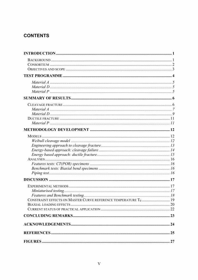
CONTENTS INTRODUCTION.................................................................................................................... 1

BACKGROUND ......................................................................................................................... 1 CONSORTIUM .......................................................................................................................... 2 OBJECTIVES AND SCOPE .......................................................................................................... 3

TEST PROGRAMME ............................................................................................................. 4

Material A .......................................................................................................................... 5 Material D.......................................................................................................................... 5 Material P .......................................................................................................................... 5

SUMMARY OF RESULTS..................................................................................................... 6 CLEAVAGE FRACTURE............................................................................................................. 6

Material A .......................................................................................................................... 7 Material D.......................................................................................................................... 9

DUCTILE FRACTURE .............................................................................................................. 11 Material P ........................................................................................................................ 11

METHODOLOGY DEVELOPMENT ................................................................................ 12 MODELS ................................................................................................................................ 12

Weibull cleavage model ................................................................................................... 12 Engineering approach to cleavage fracture..................................................................... 13 Energy-based approach: cleavage failure ....................................................................... 14 Energy based approach: ductile fracture......................................................................... 15

ANALYSES............................................................................................................................. 16 Features tests: CT(POR) specimens ................................................................................ 16 Benchmark tests: Biaxial bend specimens ....................................................................... 16 Piping test......................................................................................................................... 16

DISCUSSION ......................................................................................................................... 17 EXPERIMENTAL METHODS ..................................................................................................... 17

Miniaturised testing.......................................................................................................... 17 Features and Benchmark testing...................................................................................... 18

CONSTRAINT EFFECTS ON MASTER CURVE REFERENCE TEMPERATURE T0 ............................ 19 BIAXIAL LOADING EFFECTS ................................................................................................... 20 CURRENT STATUS OF PRACTICAL APPLICATION ..................................................................... 22

CONCLUDING REMARKS................................................................................................. 23

ACKNOWLEDGEMENTS................................................................................................... 24

REFERENCES....................................................................................................................... 25

FIGURES ................................................................................................................................ 27

VI

1

INTRODUCTION

BACKGROUND

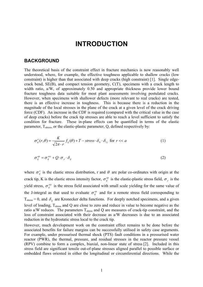
The theoretical basis of the constraint effect in fracture mechanics is now reasonably well understood, where, for example, the effective toughness applicable to shallow cracks (low constraint) is higher than that associated with deep cracks (high constraint) [1]. Single edge-crack bend, SE(B), and compact tension geometry, C(T), specimens with a crack length to width ratio, a/W, of approximately 0.50 and appropriate thickness provide lower bound fracture toughness data suitable for most plant assessments involving postulated cracks. However, when specimens with shallower defects (more relevant to real cracks) are tested, there is an effective increase in toughness. This is because there is a reduction in the magnitude of the local stresses in the plane of the crack at a given level of the crack driving force (CDF). An increase in the CDF is required (compared with the critical value in the case of deep cracks) before the crack tip stresses are able to reach a level sufficient to satisfy the condition for fracture. These in-plane effects can be quantified in terms of the elastic parameter, Tstress, or the elastic-plastic parameter, Q, defined respectively by:

jiijeij stressTf

rKr 11)(

2),( δδθ

πθσ ⋅⋅−+

⋅= for ar << (1)

ijyssyij

epij Q δσσσ ⋅⋅+= (2)

where e

ijσ is the elastic stress distribution, r and θ are polar co-ordinates with origin at the

crack tip, K is the elastic stress intensity factor, epijσ is the elastic-plastic stress field, yσ is the

yield stress, ssyijσ is the stress field associated with small scale yielding for the same value of

the J-integral as that used to evaluate epijσ and for a remote stress field corresponding to

Tstress = 0, and ijδ are Kronecker delta functions. For deeply notched specimens, and a given level of loading, Tstress and Q are close to zero and reduce in value to become negative as the ratio a/W reduces. The parameters Tstress and Q are measures of crack-tip constraint, and the loss of constraint associated with their decrease as a/W decreases is due to an associated reduction in the hydrostatic stress local to the crack tip. However, much development work on the constraint effect remains to be done before the associated benefits for failure margins can be successfully utilised in safety case arguments. For example, under pressurised thermal shock (PTS) fault conditions in a pressurised water reactor (PWR), the thermal, pressure, and residual stresses in the reactor pressure vessel (RPV) combine to form a complex, biaxial, non-linear state of stress [2]. Included in this stress field are significant tensile out-of-plane stresses aligned parallel to possible surface or embedded flaws oriented in either the longitudinal or circumferential directions. While the

2

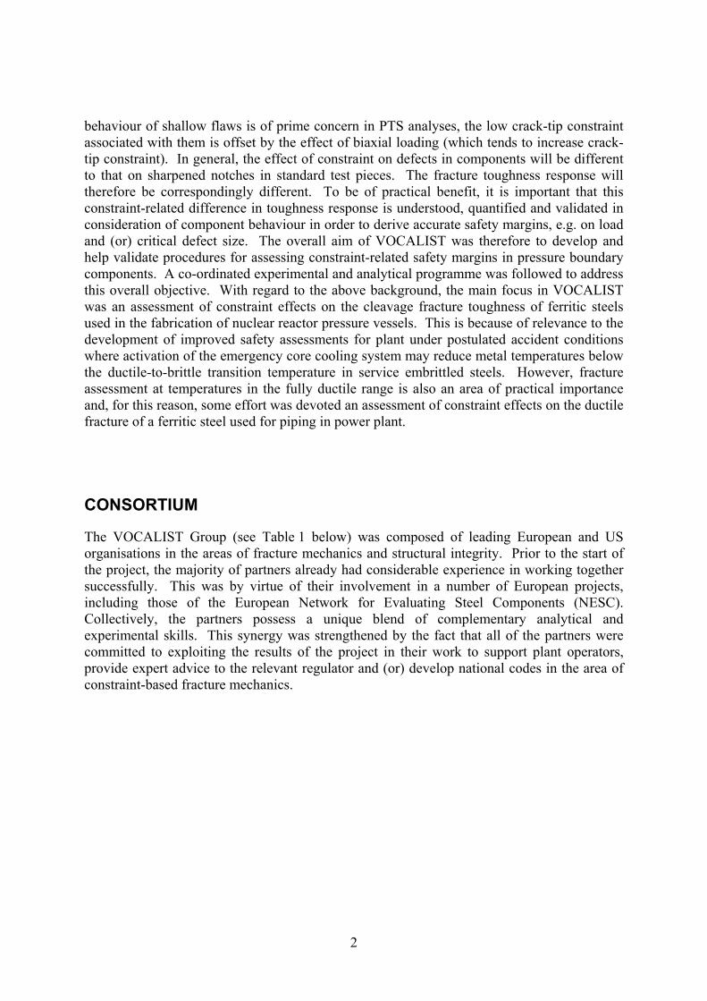
behaviour of shallow flaws is of prime concern in PTS analyses, the low crack-tip constraint associated with them is offset by the effect of biaxial loading (which tends to increase crack-tip constraint). In general, the effect of constraint on defects in components will be different to that on sharpened notches in standard test pieces. The fracture toughness response will therefore be correspondingly different. To be of practical benefit, it is important that this constraint-related difference in toughness response is understood, quantified and validated in consideration of component behaviour in order to derive accurate safety margins, e.g. on load and (or) critical defect size. The overall aim of VOCALIST was therefore to develop and help validate procedures for assessing constraint-related safety margins in pressure boundary components. A co-ordinated experimental and analytical programme was followed to address this overall objective. With regard to the above background, the main focus in VOCALIST was an assessment of constraint effects on the cleavage fracture toughness of ferritic steels used in the fabrication of nuclear reactor pressure vessels. This is because of relevance to the development of improved safety assessments for plant under postulated accident conditions where activation of the emergency core cooling system may reduce metal temperatures below the ductile-to-brittle transition temperature in service embrittled steels. However, fracture assessment at temperatures in the fully ductile range is also an area of practical importance and, for this reason, some effort was devoted an assessment of constraint effects on the ductile fracture of a ferritic steel used for piping in power plant.

CONSORTIUM

The VOCALIST Group (see Table 1 below) was composed of leading European and US organisations in the areas of fracture mechanics and structural integrity. Prior to the start of the project, the majority of partners already had considerable experience in working together successfully. This was by virtue of their involvement in a number of European projects, including those of the European Network for Evaluating Steel Components (NESC). Collectively, the partners possess a unique blend of complementary analytical and experimental skills. This synergy was strengthened by the fact that all of the partners were committed to exploiting the results of the project in their work to support plant operators, provide expert advice to the relevant regulator and (or) develop national codes in the area of constraint-based fracture mechanics.

3

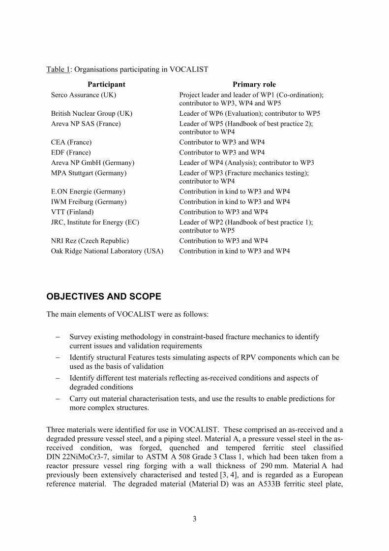
Table 1: Organisations participating in VOCALIST

Participant Primary role Serco Assurance (UK) Project leader and leader of WP1 (Co-ordination);

contributor to WP3, WP4 and WP5 British Nuclear Group (UK) Leader of WP6 (Evaluation); contributor to WP5 Areva NP SAS (France) Leader of WP5 (Handbook of best practice 2);

contributor to WP4 CEA (France) Contributor to WP3 and WP4 EDF (France) Contributor to WP3 and WP4 Areva NP GmbH (Germany) Leader of WP4 (Analysis); contributor to WP3 MPA Stuttgart (Germany) Leader of WP3 (Fracture mechanics testing);

contributor to WP4 E.ON Energie (Germany) Contribution in kind to WP3 and WP4 IWM Freiburg (Germany) Contribution in kind to WP3 and WP4 VTT (Finland) Contribution to WP3 and WP4 JRC, Institute for Energy (EC) Leader of WP2 (Handbook of best practice 1);

contributor to WP5 NRI Rez (Czech Republic) Contribution to WP3 and WP4 Oak Ridge National Laboratory (USA) Contribution in kind to WP3 and WP4

OBJECTIVES AND SCOPE

The main elements of VOCALIST were as follows:

− Survey existing methodology in constraint-based fracture mechanics to identify current issues and validation requirements

− Identify structural Features tests simulating aspects of RPV components which can be used as the basis of validation

− Identify different test materials reflecting as-received conditions and aspects of degraded conditions

− Carry out material characterisation tests, and use the results to enable predictions for more complex structures.

Three materials were identified for use in VOCALIST. These comprised an as-received and a degraded pressure vessel steel, and a piping steel. Material A, a pressure vessel steel in the as-received condition, was forged, quenched and tempered ferritic steel classified DIN 22NiMoCr3-7, similar to ASTM A 508 Grade 3 Class 1, which had been taken from a reactor pressure vessel ring forging with a wall thickness of 290 mm. Material A had previously been extensively characterised and tested [3, 4], and is regarded as a European reference material. The degraded material (Material D) was an A533B ferritic steel plate,

4

HSST Plate 14, which had been heat treated in order to produce elevated yield stress (range 620 to 655 MPa) typical of a radiation sensitive RPV steel irradiated to a fluence of 1.5 x 1019 n/cm2 (En > 1 MeV). Material P was French ferritic steel Tu52B used for piping in power plant.

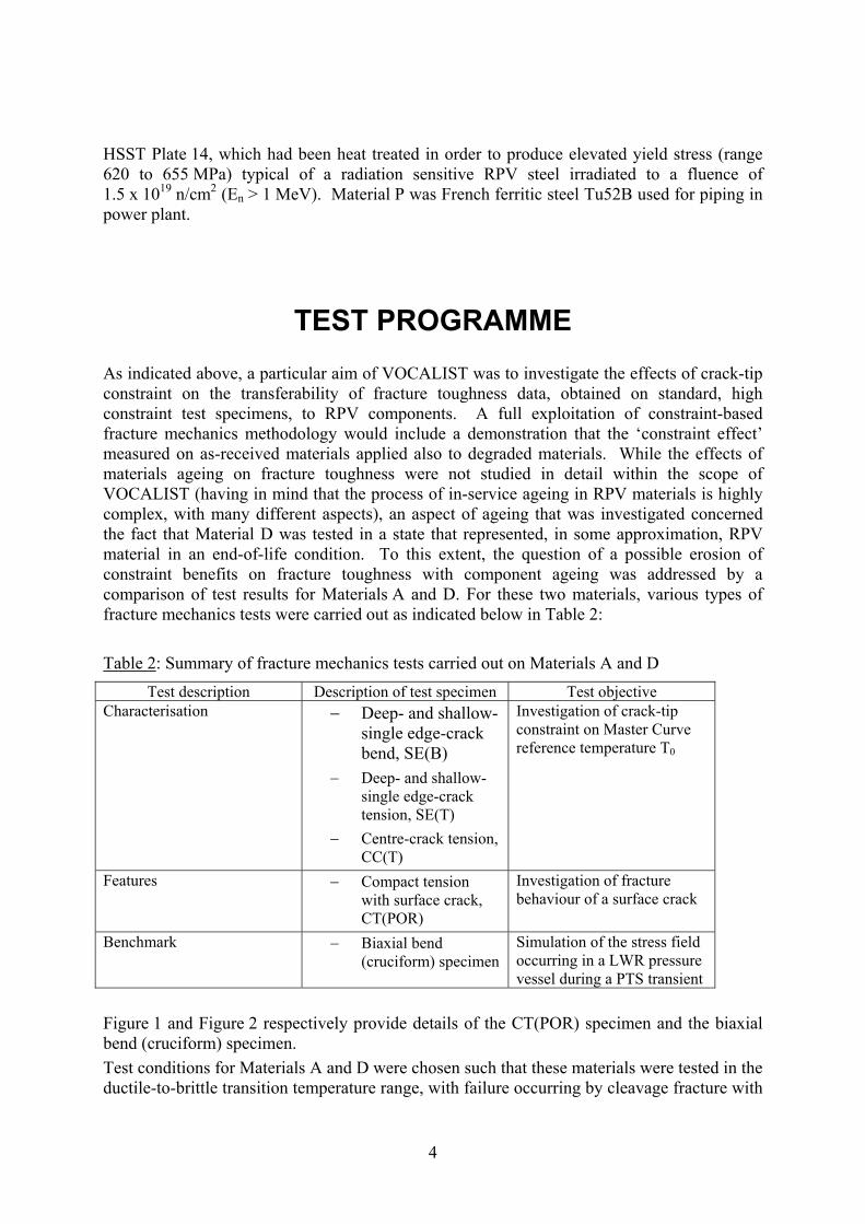
TEST PROGRAMME As indicated above, a particular aim of VOCALIST was to investigate the effects of crack-tip constraint on the transferability of fracture toughness data, obtained on standard, high constraint test specimens, to RPV components. A full exploitation of constraint-based fracture mechanics methodology would include a demonstration that the ‘constraint effect’ measured on as-received materials applied also to degraded materials. While the effects of materials ageing on fracture toughness were not studied in detail within the scope of VOCALIST (having in mind that the process of in-service ageing in RPV materials is highly complex, with many different aspects), an aspect of ageing that was investigated concerned the fact that Material D was tested in a state that represented, in some approximation, RPV material in an end-of-life condition. To this extent, the question of a possible erosion of constraint benefits on fracture toughness with component ageing was addressed by a comparison of test results for Materials A and D. For these two materials, various types of fracture mechanics tests were carried out as indicated below in Table 2: Table 2: Summary of fracture mechanics tests carried out on Materials A and D

Test description Description of test specimen Test objective Characterisation − Deep- and shallow-

single edge-crack bend, SE(B)

− Deep- and shallow-single edge-crack tension, SE(T)

− Centre-crack tension, CC(T)

Investigation of crack-tip constraint on Master Curve reference temperature T0

Features − Compact tension with surface crack, CT(POR)

Investigation of fracture behaviour of a surface crack

Benchmark − Biaxial bend (cruciform) specimen

Simulation of the stress field occurring in a LWR pressure vessel during a PTS transient

Figure 1 and Figure 2 respectively provide details of the CT(POR) specimen and the biaxial bend (cruciform) specimen. Test conditions for Materials A and D were chosen such that these materials were tested in the ductile-to-brittle transition temperature range, with failure occurring by cleavage fracture with

5

minimal pre-cleavage ductile tearing. Most of the subsequent methodology development (described below) was based on Material A data. Tests on Material P were carried out at ambient temperature, which corresponded to a temperature in the fully ductile regime. A summary of the fracture mechanics tests performed within VOCALIST on all three materials is presented below.

Material A The tests on Material A covered several types of specimen, in which absolute size (thickness B and width W), and relative crack length (a/W), were varied as follows: SE(B); B = W =25 mm, (a/W ~ 0.5 and ~ 0.1), tested at temperatures in the range -110° to

-60°C SE(B); B = W =10 mm, (a/W ~ 0.5 and ~ 0.1), tested at temperatures in the range -113° to

-110°C (a/W ~ 0.5) and -118° to -101°C (a/W ~ 0.1) SE(T); B = W =10 mm, (a/W ~ 0.5 and ~ 0.1), tested at temperatures in the range -130° to

-110°C (a/W ~ 0.5) and -150° to -120°C (a/W ~ 0.1) CC(T); B = 10 mm, 2W = 80 mm, (a/W ~ 0.7), test temperature = -110°C CT(POR); B = 50 mm, W = 100 mm, crack depth a = 6 mm and length 2c = 16 mm (crack

front length ~ 22.6 mm) tested at temperatures in the range -90° to -60°C

Biaxial bend; B = W ~ 100 mm, a/W ~ 0.1, equibiaxial loading, tested at temperatures in the range -60° to -50°C

All specimens were tested in the L-S orientation, where L = circumferential direction in the ring forging and S = radial (thickness) direction.

Material D SE(B); B = W =25 mm, (a/W ~ 0.5 and ~ 0.1), tested at temperatures in the range

-60° to -20°C (a/W ~ 0.5) and -90° to -60°C (a/W ~ 0.1) SE(B); B = W =10 mm, (a/W ~ 0.5 and ~ 0.1), tested at temperatures in the range

-60° to -20°C (a/W ~ 0.5) and -110° to -80°C (a/W ~ 0.1) SE(T); B = W =10 mm, (a/W ~ 0.5 and ~ 0.1), tested at temperatures in the range

-90° to -60°C (a/W ~ 0.5) and -110° to -80°C (a/W ~ 0.1) CT(POR); B = 50 mm, W = 100 mm, crack depth a = 6 mm and length 2c = 16 mm (crack

front length ~ 22.6 mm) tested at -40°C Biaxial bend; B = W ~ 100 mm, a/W ~ 0.1, equibiaxial loading, tested at -5°C Biaxial bend; B = W ~ 150 mm, a/W ~ 0.1, equibiaxial loading, tested at 0°C

All specimens were tested in the L-S orientation, where L = rolling direction in the plate and S = thickness direction.

Material P These tests were designed to investigate the ductile tearing occurring at circumferential defects in pipes subject to four-point bending. A through-wall defect was considered in the first test; a surface-breaking defect was considered in the second. The rig in which these

6

Benchmark tests were conducted is shown in Figure 3. In addition to Benchmark tests, a comprehensive materials characterisation programme was carried out which involved the testing of Charpy impact specimens, plain-sided and notched tensile specimens, and 12 mm- and 25 mm-thick compact fracture toughness specimens, C(T).

SUMMARY OF RESULTS

CLEAVAGE FRACTURE

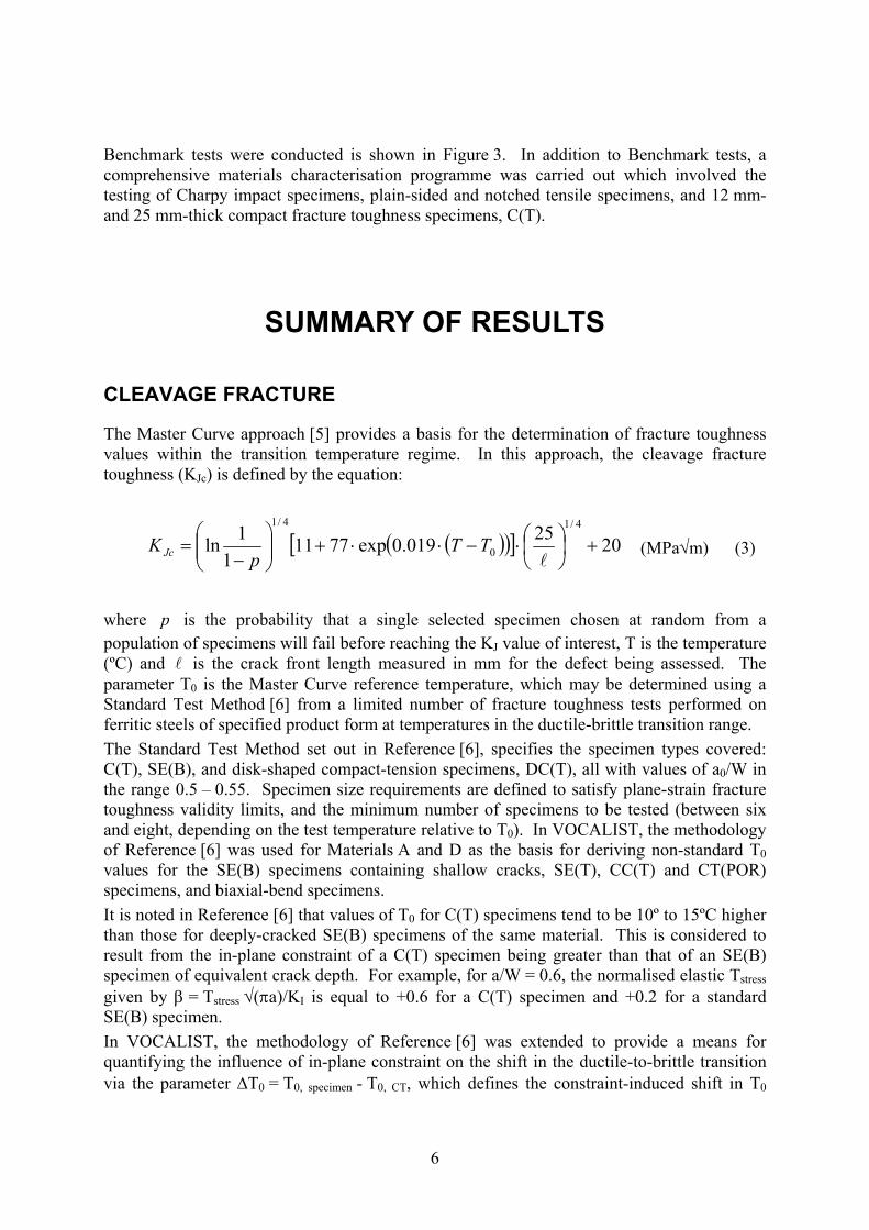
The Master Curve approach [5] provides a basis for the determination of fracture toughness values within the transition temperature regime. In this approach, the cleavage fracture toughness (KJc) is defined by the equation:

( )( )[ ] 2025019.0exp77111

1ln4/1

0

4/1

+⎟⎠⎞

⎜⎝⎛⋅−⋅⋅+⎟⎟

⎠

⎞⎜⎜⎝

⎛−

=l

TTp

K Jc (MPa√m) (3)

where p is the probability that a single selected specimen chosen at random from a population of specimens will fail before reaching the KJ value of interest, T is the temperature (ºC) and l is the crack front length measured in mm for the defect being assessed. The parameter T0 is the Master Curve reference temperature, which may be determined using a Standard Test Method [6] from a limited number of fracture toughness tests performed on ferritic steels of specified product form at temperatures in the ductile-brittle transition range. The Standard Test Method set out in Reference [6], specifies the specimen types covered: C(T), SE(B), and disk-shaped compact-tension specimens, DC(T), all with values of a0/W in the range 0.5 – 0.55. Specimen size requirements are defined to satisfy plane-strain fracture toughness validity limits, and the minimum number of specimens to be tested (between six and eight, depending on the test temperature relative to T0). In VOCALIST, the methodology of Reference [6] was used for Materials A and D as the basis for deriving non-standard T0 values for the SE(B) specimens containing shallow cracks, SE(T), CC(T) and CT(POR) specimens, and biaxial-bend specimens. It is noted in Reference [6] that values of T0 for C(T) specimens tend to be 10º to 15ºC higher than those for deeply-cracked SE(B) specimens of the same material. This is considered to result from the in-plane constraint of a C(T) specimen being greater than that of an SE(B) specimen of equivalent crack depth. For example, for a/W = 0.6, the normalised elastic Tstress given by β = Tstress √(πa)/KI is equal to +0.6 for a C(T) specimen and +0.2 for a standard SE(B) specimen. In VOCALIST, the methodology of Reference [6] was extended to provide a means for quantifying the influence of in-plane constraint on the shift in the ductile-to-brittle transition via the parameter ∆T0 = T0, specimen - T0, CT, which defines the constraint-induced shift in T0

7

relative to the high constraint C(T) transition curve. This approach assumes that the transition curve shape remains unchanged by constraint loss. Whilst this may not strictly be the case over the full transition temperature range, this assumption is considered reasonable within the requirements of Reference [6] for measurement of a valid reference temperature (T0 ± 50ºC).

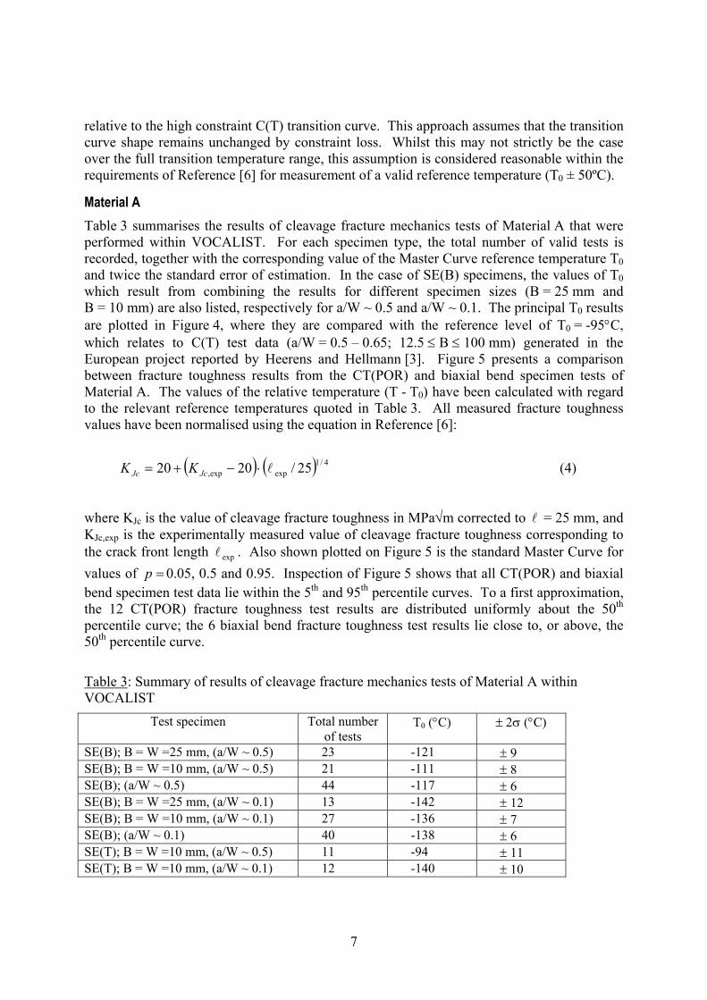
Material A Table 3 summarises the results of cleavage fracture mechanics tests of Material A that were performed within VOCALIST. For each specimen type, the total number of valid tests is recorded, together with the corresponding value of the Master Curve reference temperature T0 and twice the standard error of estimation. In the case of SE(B) specimens, the values of T0 which result from combining the results for different specimen sizes (B = 25 mm and B = 10 mm) are also listed, respectively for a/W ~ 0.5 and a/W ~ 0.1. The principal T0 results are plotted in Figure 4, where they are compared with the reference level of T0 = -95°C, which relates to C(T) test data (a/W = 0.5 – 0.65; 12.5 ≤ B ≤ 100 mm) generated in the European project reported by Heerens and Hellmann [3]. Figure 5 presents a comparison between fracture toughness results from the CT(POR) and biaxial bend specimen tests of Material A. The values of the relative temperature (T - T0) have been calculated with regard to the relevant reference temperatures quoted in Table 3. All measured fracture toughness values have been normalised using the equation in Reference [6]:

( ) ( ) 4/1expexp, 25/2020 l⋅−+= JcJc KK (4)

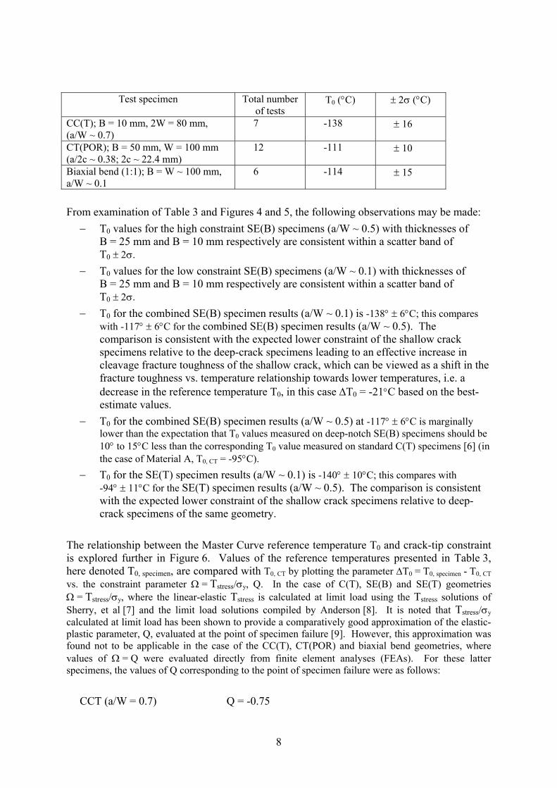
where KJc is the value of cleavage fracture toughness in MPa√m corrected to l = 25 mm, and KJc,exp is the experimentally measured value of cleavage fracture toughness corresponding to the crack front length expl . Also shown plotted on Figure 5 is the standard Master Curve for values of =p 0.05, 0.5 and 0.95. Inspection of Figure 5 shows that all CT(POR) and biaxial bend specimen test data lie within the 5th and 95th percentile curves. To a first approximation, the 12 CT(POR) fracture toughness test results are distributed uniformly about the 50th percentile curve; the 6 biaxial bend fracture toughness test results lie close to, or above, the 50th percentile curve. Table 3: Summary of results of cleavage fracture mechanics tests of Material A within VOCALIST

Test specimen Total number of tests

T0 (°C) ± 2σ (°C)

SE(B); B = W =25 mm, (a/W ~ 0.5) 23 -121 ± 9 SE(B); B = W =10 mm, (a/W ~ 0.5) 21 -111 ± 8 SE(B); (a/W ~ 0.5) 44 -117 ± 6 SE(B); B = W =25 mm, (a/W ~ 0.1) 13 -142 ± 12 SE(B); B = W =10 mm, (a/W ~ 0.1) 27 -136 ± 7 SE(B); (a/W ~ 0.1) 40 -138 ± 6 SE(T); B = W =10 mm, (a/W ~ 0.5) 11 -94 ± 11 SE(T); B = W =10 mm, (a/W ~ 0.1) 12 -140 ± 10

8

Test specimen Total number of tests

T0 (°C) ± 2σ (°C)

CC(T); B = 10 mm, 2W = 80 mm, (a/W ~ 0.7)

7 -138 ± 16

CT(POR); B = 50 mm, W = 100 mm (a/2c ~ 0.38; 2c ~ 22.4 mm)

12 -111 ± 10

Biaxial bend (1:1); B = W ~ 100 mm, a/W ~ 0.1

6 -114 ± 15

From examination of Table 3 and Figures 4 and 5, the following observations may be made:

− T0 values for the high constraint SE(B) specimens (a/W ~ 0.5) with thicknesses of B = 25 mm and B = 10 mm respectively are consistent within a scatter band of T0 ± 2σ.

− T0 values for the low constraint SE(B) specimens (a/W ~ 0.1) with thicknesses of B = 25 mm and B = 10 mm respectively are consistent within a scatter band of T0 ± 2σ.

− T0 for the combined SE(B) specimen results (a/W ~ 0.1) is -138° ± 6°C; this compares with -117° ± 6°C for the combined SE(B) specimen results (a/W ~ 0.5). The comparison is consistent with the expected lower constraint of the shallow crack specimens relative to the deep-crack specimens leading to an effective increase in cleavage fracture toughness of the shallow crack, which can be viewed as a shift in the fracture toughness vs. temperature relationship towards lower temperatures, i.e. a decrease in the reference temperature T0, in this case ∆T0 = -21°C based on the best-estimate values.

− T0 for the combined SE(B) specimen results (a/W ~ 0.5) at -117° ± 6°C is marginally lower than the expectation that T0 values measured on deep-notch SE(B) specimens should be 10° to 15°C less than the corresponding T0 value measured on standard C(T) specimens [6] (in the case of Material A, T0, CT = -95°C).

− T0 for the SE(T) specimen results (a/W ~ 0.1) is -140° ± 10°C; this compares with -94° ± 11°C for the SE(T) specimen results (a/W ~ 0.5). The comparison is consistent with the expected lower constraint of the shallow crack specimens relative to deep-crack specimens of the same geometry.

The relationship between the Master Curve reference temperature T0 and crack-tip constraint is explored further in Figure 6. Values of the reference temperatures presented in Table 3, here denoted T0, specimen, are compared with T0, CT by plotting the parameter ∆T0 = T0, specimen - T0, CT vs. the constraint parameter Ω = Tstress/σy, Q. In the case of C(T), SE(B) and SE(T) geometries Ω = Tstress/σy, where the linear-elastic Tstress is calculated at limit load using the Tstress solutions of Sherry, et al [7] and the limit load solutions compiled by Anderson [8]. It is noted that Tstress/σy calculated at limit load has been shown to provide a comparatively good approximation of the elastic-plastic parameter, Q, evaluated at the point of specimen failure [9]. However, this approximation was found not to be applicable in the case of the CC(T), CT(POR) and biaxial bend geometries, where values of Ω = Q were evaluated directly from finite element analyses (FEAs). For these latter specimens, the values of Q corresponding to the point of specimen failure were as follows:

CCT (a/W = 0.7) Q = -0.75

9

CT(POR) (a/W = 0.085) Q = -0.4 Biaxial-bend (a/W = 0.1) Q = -0.6

Also shown plotted in Figure 6 is ∆T0 = T0, Ω - T0, CT vs. Ω, where, following Reference [9]:

yTT σλ

⋅⎟⎠⎞

⎜⎝⎛ Ω

+= =Ω 00 (5)

and where T0, CT = -95°C [3] and λ = 12 MPa°C-1. The value of T0, Ω=0 = -118°C in Figure 6 is set so as to enable the trend line to pass through the data point corresponding to high constraint specimens, C(T) (a/W = 0.55); σy = 580 MPa, and corresponds to the average yield stress of Material A over the range of test temperatures considered. The value of the trend line slope λ = 12 MPa°C-1 in Equation (5) represents a recent revision by Wallin during the course of project VOCALIST to the value λ = 10 MPa°C-1 originally quoted by this author in Reference [9]. Inspection of Figure 6 shows that the above trend line, with an approximate 2 standard deviations scatter band of ± 10°C, provides an approximate guide to the behaviour of deep- and shallow-notch SE(B) specimens, and shallow-notch SE(T) specimens, relative to deep-notch C(T) specimens. For the other geometries considered (deep-notch SE(T), CT(POR), shallow-notch biaxial bend, and deep-notch CC(T) specimens), the trend line overestimates the shift in transition temperature with crack-tip constraint relative to that of the deep-notch C(T) specimens.

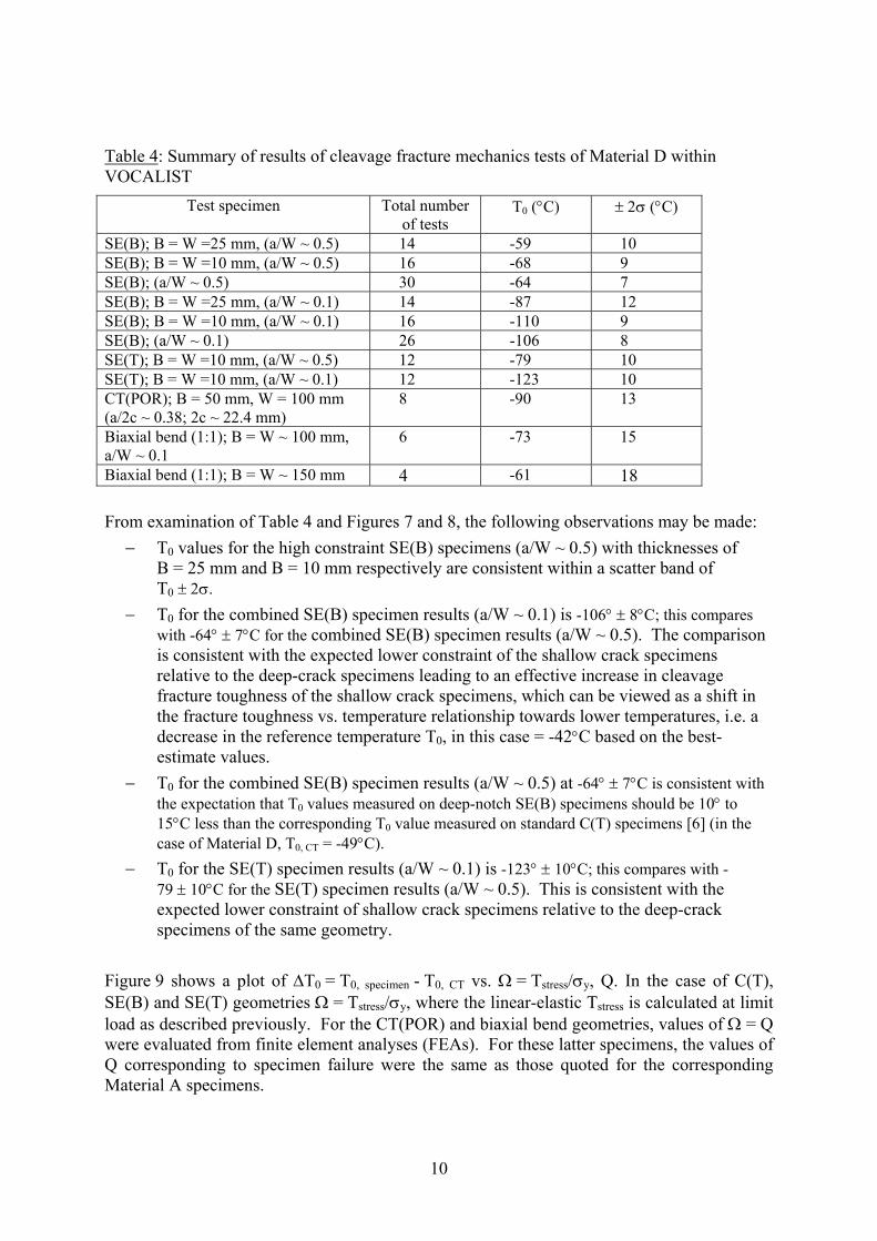
Material D Table 4 summarises the results of cleavage fracture mechanics tests of Material D that were performed within VOCALIST. For each specimen type, the total number of valid tests is recorded, together with the corresponding value of the Master Curve reference temperature T0 and twice the standard error of estimation. In the case of SE(B) specimens, the values of T0 which result from combining the results for different specimen sizes (B = 25 mm and B = 10 mm) are also listed, respectively for a/W ~ 0.5 and a/W ~ 0.1. The principal T0 results are plotted in Figure 7, where they are compared with the reference level of T0 = -49°C, which relates to C(T) test data (a/W = 0.5, B = 12.5 mm) reported by Bass, et al [10]. Figure 8 compares fracture toughness results from the CT(POR) and biaxial bend specimen tests of Material D. The values of the relative temperature (T - T0) have been calculated with regard to the relevant reference temperatures quoted in Table 4. All measured fracture toughness values have been size corrected to l = 25 mm using Equation (4). Inspection of Figure 8 shows that all but one of the CT(POR) specimen results, and all but one of the 100 mm x 100 mm biaxial bend specimen results, lie within the 5th and 95th percentile Master Curves. To a first approximation, all test data are distributed uniformly about the 50th percentile curve.

10

Table 4: Summary of results of cleavage fracture mechanics tests of Material D within VOCALIST

Test specimen Total number of tests

T0 (°C) ± 2σ (°C)

SE(B); B = W =25 mm, (a/W ~ 0.5) 14 -59 10 SE(B); B = W =10 mm, (a/W ~ 0.5) 16 -68 9 SE(B); (a/W ~ 0.5) 30 -64 7 SE(B); B = W =25 mm, (a/W ~ 0.1) 14 -87 12 SE(B); B = W =10 mm, (a/W ~ 0.1) 16 -110 9 SE(B); (a/W ~ 0.1) 26 -106 8 SE(T); B = W =10 mm, (a/W ~ 0.5) 12 -79 10 SE(T); B = W =10 mm, (a/W ~ 0.1) 12 -123 10 CT(POR); B = 50 mm, W = 100 mm (a/2c ~ 0.38; 2c ~ 22.4 mm)

8 -90 13

Biaxial bend (1:1); B = W ~ 100 mm, a/W ~ 0.1

6 -73 15

Biaxial bend (1:1); B = W ~ 150 mm 4 -61 18 From examination of Table 4 and Figures 7 and 8, the following observations may be made:

− T0 values for the high constraint SE(B) specimens (a/W ~ 0.5) with thicknesses of B = 25 mm and B = 10 mm respectively are consistent within a scatter band of T0 ± 2σ.

− T0 for the combined SE(B) specimen results (a/W ~ 0.1) is -106° ± 8°C; this compares with -64° ± 7°C for the combined SE(B) specimen results (a/W ~ 0.5). The comparison is consistent with the expected lower constraint of the shallow crack specimens relative to the deep-crack specimens leading to an effective increase in cleavage fracture toughness of the shallow crack specimens, which can be viewed as a shift in the fracture toughness vs. temperature relationship towards lower temperatures, i.e. a decrease in the reference temperature T0, in this case = -42°C based on the best-estimate values.

− T0 for the combined SE(B) specimen results (a/W ~ 0.5) at -64° ± 7°C is consistent with the expectation that T0 values measured on deep-notch SE(B) specimens should be 10° to 15°C less than the corresponding T0 value measured on standard C(T) specimens [6] (in the case of Material D, T0, CT = -49°C).

− T0 for the SE(T) specimen results (a/W ~ 0.1) is -123° ± 10°C; this compares with -79 ± 10°C for the SE(T) specimen results (a/W ~ 0.5). This is consistent with the expected lower constraint of shallow crack specimens relative to the deep-crack specimens of the same geometry.

Figure 9 shows a plot of ∆T0 = T0, specimen - T0, CT vs. Ω = Tstress/σy, Q. In the case of C(T), SE(B) and SE(T) geometries Ω = Tstress/σy, where the linear-elastic Tstress is calculated at limit load as described previously. For the CT(POR) and biaxial bend geometries, values of Ω = Q were evaluated from finite element analyses (FEAs). For these latter specimens, the values of Q corresponding to specimen failure were the same as those quoted for the corresponding Material A specimens.

11

Also shown plotted in Figure 9 is ∆T0 = T0, Ω - T0, CT vs. Ω where, for Material D, the parameters in Equation (5) are T0, CT = -49°C, λ = 12 MPa°C-1 as before, the reference temperature T0, Ω=0 = -76°C and the average yield stress σy = 676 MPa. Inspection of Figure 9 shows that the calibrated Equation (5) trend line, with an approximate 2 standard deviations scatter band of ± 10°C, provides a reasonable guide to the behaviour of the deep- and shallow-notch SE(B) specimens, deep- and shallow-notch SE(T) specimens, and the CT(POR) specimens, relative to deep-notch C(T) specimens. For the shallow-notch biaxial bend specimens (100 mm x 100 mm and 150 mm x 150 mm), the trend line overestimates the shift in transition temperature with crack-tip constraint relative to that of the deep-notch C(T) specimens.

DUCTILE FRACTURE

Material P The large-scale tests carried out on Material P were designed to investigate the effect of crack-tip constraint on the ductile tearing behaviour of circumferential defects in pipes subjected to four-point loading in bend. Two Benchmark tests were carried out. In the first test a through-wall defect was considered. The central test section was 236 mm long, with an outside diameter of 220 mm and a wall thickness of 15 mm. This section contained a circumferential machined slot, which subtended an angle 2β ~ 90° in the radial plane. The ends of the slot were sharpened by fatigue. The dimensions of the initial crack were measured on the final fracture surface as summarised in Table 5 below. Table 5: Crack sizes after fatigue pre-cracking in first Benchmark test of Material P ∆a - average ∆a – inner wall ∆a – outer wall θ average (°) Notch at +45° 8.8 mm 9.6 mm 8 mm +49.9 Notch at –45° 11.4 mm 12 mm 10.8 mm -51.4 The first test resulted in a significant amount of stable ductile tearing at the ends of the through-wall circumferential crack. Table 6 summarises the crack lengths measured by the potential drop technique during the test. The maximum bending moment reached was 124.6 kNm. Figure 3(a) shows a photograph of the central section of the test assembly; Figure 3(b) shows a photograph of the test rig. Table 6: Measurements of ductile crack growth in first Benchmark test of Material P ∆a - maximum ∆a – inner wall ∆a – outer wall θ maximum (°) Notch at +45° 26.4 mm 20 mm 21.6 mm +64.7 Notch at –45° 28.8 mm 26.4 mm 26.4 mm -67.5 The second test was on a pipe with an external part-circumferential surface-breaking defect introduced by spark erosion (length 2c = 50.1 mm, depth a = 8.1 mm) and sharpened by fatigue. A larger load was required to deform the pipe than that used in the first test. Unfortunately, problems with a hydraulic pump prevented the load being raised sufficiently to

12

cause crack initiation. However, the maximum load reached was sufficient to cause significant plastic deformation, and this enabled theoretical methods for calculating the load-displacement relationship for the defective pipe to be validated.

METHODOLOGY DEVELOPMENT A number of methodologies for the assessment of constraint effects on fracture behaviour were the subject of considerable study and development within VOCALIST. Of particular importance was a critical assessment of the robustness of such methodologies in using the results obtained from small-scale (or miniature) laboratory tests for predicting the fracture behaviour of both Features and Benchmark tests. The methodologies are described below.

MODELS

Weibull cleavage model The statistical cleavage model developed by Beremin [11] has been widely used to describe the cleavage fracture behaviour of ferritic steels within the transition temperature regime. The model is based on Weibull failure statistics in which the probability of cleavage Pf is represented by either a two- or three-parameter expression of the form:

⎪⎭

⎪⎬⎫

⎪⎩

⎪⎨⎧

⎟⎟⎠

⎞⎜⎜⎝

⎛−−=

m

u

WfP

σσ

exp1 (6a)

or

⎪⎭

⎪⎬⎫

⎪⎩

⎪⎨⎧

⎟⎟⎠

⎞⎜⎜⎝

⎛−−

−−=−

−

m

Wu

WWfP

min

minexp1σσσσ

(6b)

where σW is the Weibull stress, a volume integral of stress within the fracture process zone, σW-min is the value of σW corresponding to a crack driving force of 20 MPa√m (i.e. Kmin within the Master Curve approach). The parameters m and σu represent the shape and scale parameters within the Weibull model, and are deemed to be material parameters which are independent of crack-tip constraint, but which may vary with temperature. The Weibull stress is conventionally derived from the distribution of maximum principal stress (σ1) within the plastic zone ahead of the crack. Williams et al. [12] have suggested that replacing σ1 with the hydrostatic stress, σH, to calculate the parameter QH (i.e. Q → QH, the so-called hydrostatic Q-stress) provides an improved prediction of out-of-plane constraint effects on fracture toughness, i.e. provides a means for predicting the influence of out-of-plane biaxial loading (loading parallel to the crack front) on fracture toughness.

13

Calibration of parameters in the Weibull cleavage model is a key requirement for its successful application, and work undertaken by Gao et al. [13] has provided a clear methodology for calibration against a combined reference dataset of high and low constraint fracture toughness data. This approach was adopted and Table 7 summarises the Weibull parameters derived for Material A within VOCALIST. Whilst there is relatively little scatter in the shape parameter m, the scale parameter σu varies between 1,649 and 2,062 MPa. This variation in the Weibull scale parameter is attributed to differences in the reference datasets used as the basis for calibration, whether a two- or a three-parameter Weibull model was used, and (or) whether σ1 or the σH was referenced in the calculation of Weibull stress. Table 7: Weibull cleavage model parameters derived for Materials A Calbn. m σu, MPa σW-min, MPa Reference dataset A. + 6.30 1,649 460 − SE(B) a/W ≈ 0.1 and 0.5

− Specimen data for W = B = 10 mm

− T = -90ºC B.* 5.62 2,062 667 − SE(B) a/W ≈ 0.1 and 0.5

− Statistically generated dataset from Master Curve.

− T = -60ºC C. 6.23 1,840 - − SE(B) a/W ≈ 0.1 and 0.5

− Specimen data for W = B = 10 mm

− T = -110ºC + Scale parameter includes σw-min for consistency with Eqn (4) above. * σW based on hydrostatic stress. Once calibrated, the Weibull model was used to predict the behaviour of the Features and Benchmark tests of Material A. Two approaches were used to undertake these predictions. First, using calibrations A and B, a 3D finite element analysis (FEA) was performed for the relevant specimen geometry, and the local crack-tip stresses so derived were used to calculate σW and hence Pf as a function of the crack driving force. Second, using calibration C, an engineering approach was adopted for Material A, as described in the next sub section. For Material D, Bass et al. [14] have defined m and σu as 12.65 and 2,851 MPa respectively via 3D FEA of biaxial bend specimen data. Using these data, an engineering approach was also adopted for Material D.

Engineering approach to cleavage fracture Within the R6 defect assessment method [15], the influence of crack-tip constraint on cleavage fracture toughness is defined with respect to two material parameters, α and k, such that the constraint-dependent fracture toughness mat

cK is represented by the following equations:

matcmat KK = for 0,/ ≥QT ystress σ , and (7a)

14

( ) krmat

cmat LKK βα −+= 1 for 0,/ <QT ystress σ (7b)

where Kmat is the cleavage fracture toughness under high constraint conditions for a given Pf and l . The parameter β is a measure of structural constraint, being defined either in terms of the linear-elastic Tstress or the elastic-plastic parameter, Q. The material parameters α and k may be defined with respect to cleavage fracture toughness data derived from tests on high and low constraint geometries, or via the solutions published by Sherry et al. [16, 17] which define α and k as a function of the yield, flow and fracture properties of the material of interest, i.e. Young’s modulus, E, yield stress, σy, work hardening coefficient, n, and the Weibull shape parameter, m. Using the methods detailed in Reference [17], values of α and k may be derived as functions of n, m and E/σy using the following equations:

r

p pq pr

yqp

pqr

EmnC∑∑∑= = =

⎟⎟⎠

⎞⎜⎜⎝

⎛⎟⎠⎞

⎜⎝⎛

⎟⎠⎞

⎜⎝⎛=

4

0

4 4

7502020σ

α (8a)

r

p pq pr

yqp

pqr

EmnDk ∑∑∑= = =

⎟⎟⎠

⎞⎜⎜⎝

⎛⎟⎠⎞

⎜⎝⎛

⎟⎠⎞

⎜⎝⎛=

4

0

4 4

7502020σ

(8b)

where the coefficients pqrC and pqrD are tabulated in Reference [17].

The results of the calculations of values of α and k for Materials A and D are tabulated below: Table 8: Values of α and k for Materials A and D

Tstress Q Material m n E/σy α k α k A 6.23+ 10 360 1.163 2.074 0.796 1.694 D 12.65* 12 310 4.045 2.303 2.254 1.759

+ From Reference [17] * From Reference [14] These parameters, used alongside the Master Curve description of Kmat, provide the means for predicting the Benchmark and Features tests, using the values of α and k defined with respect to the Tstress or Q.

Energy-based approach: cleavage failure The Francfort and Marigo theory generalises the Griffith brittle fracture theory to predict the initiation and sudden propagation of cracks, using an energy minimisation principle [18]. An increment of crack extension, ∆a, minimises the total energy of the structure including the energy dissipated during the propagation, and an energy release rate, Gp, can be defined. The energy minimisation is equivalent to the maximization of the function Gp(∆a) calculated as

15

the maximum of the elastic energy, integrated over a volume, Ze, encompassing the increment of crack extension, and normalised by ∆a, i.e.

⎥⎥⎦

⎤

⎢⎢⎣

⎡∆⎟⎟

⎠

⎞⎜⎜⎝

⎛= ∫∆

adawGZe

eap .max (9)

The statistical nature of cleavage failure is accounted for through a fracture probability, similar to Equation (6a) as follows:

⎥⎥

⎦

⎤

⎢⎢

⎣

⎡

⎟⎟⎠

⎞⎜⎜⎝

⎛⋅−−=

2'

'exp1m

pc

pf G

GaP (10)

where a′ and m′ are material constants calibrated against experimental data and Gpc is the critical value of Gp (the Weibull scale parameter). The approach is capable of describing brittle fracture [19], and within VOCALIST was applied to the analysis of constraint effects.

Energy based approach: ductile fracture For ductile fracture, the Ji-Gfr approach of Marie and Chapuliot [20] was considered. Within this approach, Ji is initiation toughness, determined from stretch zone width. The parameter Gfr is the energy release rate per unit of crack extension that has to be dissipated in front of the crack tip to damage the material and initiate crack extension. The parameter Gfr is derived from an FEA of a reference test (in this case C(T) tests) using several different crack lengths, bounding the range of ductile crack growth observed. As described in Reference [20], the energy dissipated during crack extension is calculated by relating the measured load-displacement curve from the reference test with numerically calculated curves for each crack length. The model parameters were identified for Material P via tests performed on C(T) specimens of thickness 12.5 mm. The initiation toughness was defined as 100 kJ/m2 and Gfr as 84 MPa. Rousselier ductile damage model The Rousselier model of ductile tearing incorporates the influence of void initiation, growth and coalescence into the constitutive equation governing material flow behaviour [21]. The plastic potential is defined as follows:

( ) 0exp1

* =−⎟⎟⎠

⎞⎜⎜⎝

⎛⋅⋅⋅+=Φ pRDf Heq

ρσσσ

ρσ

(11)

where σeq is the von Mises equivalent stress, σH is the hydrostatic stress, R(p) is the undamaged material flow stress, f is the volume fraction of voids, σ* is the stress which characterises the resistance of the matrix to the growth and coalescence of voids, D is a constant and ρ is a function of f and f0, the current and initial void volume fractions

16

respectively. Additional parameters inherent in the approach are fc, which is the critical volume fraction for void coalescence, and λmesh, which is the crack-tip mesh size. Using a series of elastic-plastic FEA of both notched tensile and C(T) specimens, the parameters derived for Material P were as follows [22]: D = 2, f0 = 5 × 10-5, σ* = 300 MPa, fc = 0.05 and λmesh = 0.15 mm.

ANALYSES

Features tests: CT(POR) specimens Figure 10 shows a comparison between the Material A CT(POR) Features test data and the Weibull model predictions. The predictions were undertaken using the Weibull cleavage fracture model with reference to Calibrations A and C, the former through a full 3D FEA and the latter applied via the engineering approach with T0 = -111ºC, and l = 15 mm defining Kmat in Equations (7a, b). Here, l was equated with the sector, symmetrical about the deepest point, of highest constraint along the semi-elliptical crack front. Both predictions provide a good description of the data over the full range of cleavage probability.

Benchmark tests: Biaxial bend specimens The predicted cumulative distributions of KJC values for the Material A biaxial bend Benchmark tests are presented in Figure 11. The Master Curve description of the high constraint C(T) specimen data for B = 25 mm is included for comparison. Predictions of the Benchmark tests were undertaken using the Weibull cleavage fracture model with respect to Calibrations A, B and C. Weibull cleavage model predictions were undertaken with respect to Calibrations A and B via full 3D FEAs. Calibration C was used for the engineering approach prediction with T0 = -117ºC (the reference temperature for deep-notch, uniaxially loaded bend specimens) and l = 112 mm (the crack-front length of the biaxial bend specimens) defining Kmat in Equations (7a, b). In addition, the results obtained using the energy-based approach to cleavage fracture are included. All Weibull model predictions provide a reasonable fit to the experimental data, with Calibration B providing a marginally better prediction of the data for Pf < 0.5 and Calibration A providing an improved prediction for Pf > 0.5. The engineering approach provides a prediction that is slightly lower for Pf < 0.5, most probably due to the fact that this analysis employed a two-parameter Weibull model, while the other analyses used a three-parameter Weibull model, Equation (6b). For Pf > 0.5, the engineering approach prediction falls between the 3D FEA predictions. By comparison, the energy-based approach provides a prediction that falls approximately 20 to 30 MPa√m below the data over the full range of cleavage probability.

Piping test Predictions of the first piping test were performed using the energy approach of Marie and Chapuliot [20] and the Rousselier ductile damage model [21]. The results in terms of predicted moment versus ductile crack extension are illustrated in Figure 12. Both approaches provided similar predictions of the critical applied moment, Mi, for ductile crack initiation. The actual initiation moment was estimated at just less than 75 kNm. The

17

energy-based approach yielded a prediction of 75.5 kNm, whilst the Rousselier model gave a prediction of 75.7 kNm. This latter prediction was found to be sensitive to the crack-tip mesh size, λmesh, with the largest value of λmesh yielding the largest predicted Mi. The variation of Mi with mesh size was 75.7, 86.9 and 109.1 kNm for λmesh = 0.15, 0.30 and 0.45 mm, respectively, suggesting a convergence of Mi to the true value (~75.7 kNm) with decreasing mesh size. For the early stages ductile crack extension, ∆a ≤ 1.0 mm, both approaches over-estimated the extent of tearing for a given applied moment. For a given load, the energy-based approach predicted slightly higher amounts of crack growth than the Rousselier model. This would be conservative for assessment purposes. For larger amounts of ductile crack extension, ∆a > 1.0 mm, the predictions agree well with the experimental data. It is noteworthy that the energy-based approach has the ability to predict larger amounts of crack growth than the Rousselier model. This limitation of Rousselier model is due to difficulties associated with numerical convergence of the finite element calculation at large amounts of crack growth. Classical J-∆a methodology was also applied to prediction of the first piping test, giving similar results to the predictions of the Ji-Gfr and Rousselier approaches. The J-∆a methodology predicted the maximum applied bending moment well, but it tended to underestimate the load at a given displacement beyond this point. Whilst predictions of initiation and ductile crack extension were performed for the second piping test, there were no experimental data with which to compare the predictions. In general, the trends predicted for the first test were reproduced in the second test. In particular, the initiation moment predicted by the energy-based approach agreed with the prediction of the Rousselier model, when the latter was used with λmesh = 0.15 mm. As in the analysis of the first piping test, the initiation moment predicted by the Rousselier model was dependent on crack-tip mesh size; similarly, the energy-based approach predicted a slightly greater amount of tearing than the Rousselier model for a given applied moment.

DISCUSSION

EXPERIMENTAL METHODS

Miniaturised testing One aspect of the matrix of fracture mechanics tests performed under VOCALIST was to allow the Master Curve reference temperature, T0, determined from tests on sub-sized specimens (B = 10 mm) to be compared with the value obtained from tests on full sized specimens (B ≥ 25 mm). It has already been noted that for both Materials A and D, T0 values for high constraint SE(B) specimens (a/W ~ 0.5) with thicknesses of B = 10 mm and B = 25 mm respectively were consistent within a scatter band of T0 ± 2σ. In the case of Material A it was possible to compare T0 obtained from testing 10 mm-thick, deep-notch

18

SE(B) specimens (-111° ± 8°C) with the value obtained from testing standard C(T) specimens up to 100 mm in thickness (T0 = -95°C). Allowing for an anticipated shift T0, SE(B) - T0, CT of up to -15°C [6], the two values agree very well, adding some confidence in the use of sub-sized specimens for Master Curve reference temperature determinations. However, despite this agreement, there are some inconsistencies which should be noted. Figure 13 compares reference temperatures, T0, for SE(B) specimens of Material A with thicknesses of B = 25mm and B = 10mm. Figure 14 makes similar comparisons for Material D. It might be expected that the 10mm-thick specimens would exhibit somewhat lower values of T0 compared with the 25mm-thick specimens [13] since, with increasing levels of crack driving force, 10mm-thick specimens would lose constraint, due to a relaxation of out-of-plane crack-tip stresses, more rapidly than 25mm-thick specimens. This expectation is borne out for Material D in Figure 14, but the opposite trend is observed in the case of Material A in Figure 13. The use of pre-cracked Charpy specimens in surveillance testing is of course an important aspect of applying Master Curve methodology to the assessment of irradiated RPV ferritic steels. Notwithstanding the above remarks, the results within VOCALIST demonstrate that tests on 10 mm-thick, deep-notch SE(B) specimens of Materials A and D at relative temperatures in the range -50° ≤ T-T0 ≤ +50°C produced values of T0 that are consistent (within 10°C) with the corresponding values obtained by testing 25 mm-thick specimens. It is noted that Material D was specially heat treated so as to simulate the elevation in yield stress expected of radiation sensitive RPV steel irradiated to a fluence of 1.5 x 1019 n/cm2 (En > 1 MeV). To this extent, the results provide some added confidence to applications of the Master Curve procedure to the analysis of pre-cracked Charpy specimen data obtained in surveillance testing of irradiated RPV steels.

Features and Benchmark testing A particular objective of VOCALIST was to investigate the extent to which the Master Curve procedure is able to provide an adequate description of cleavage fracture toughness for non-standard geometries as a function of temperature in the ductile brittle transition range. The CT(POR) specimen was used as a Features test to investigate whether a relatively small specimen could be used to investigate the cleavage behaviour of a surface crack. The biaxial bend specimen was used as a Benchmark test to investigate shallow crack behaviour under loading conditions that simulate some aspects of the stress field occurring in a PWR vessel during a PTS transient. In all cases, the Features and Benchmark tests achieved the objective of terminating in brittle fracture, with minimal pre-cleavage ductile tearing. There are two aspects relating to the application of the Master Curve procedure to these test data: (i) definition of T0 for a non-standard geometry and, in the case of the biaxial bend specimen, non-standard loading conditions; (ii) comparison of Features and Benchmark test data normalised to l = 25 mm with the standard Master Curves (p = 0.05, 0.5 and 0.95) over a given temperature range relative to T0. These comparisons are made in Figures 5 and 8 for Material A and Material D test data respectively. It has already been noted that these data are indeed described adequately by the Master Curve description of cleavage toughness vs. relative temperature, T - T0. In the case of Material A, the comparison of the normalised test data with the standard Master Curves is over the approximate temperature range -20° ≤ T - T0 ≤ +60°C. For Material D the range for comparison is somewhat narrower, +50° ≤ T - T0 ≤ +70°C. Collectively, the data presented in Figures 5 and 8 provide confidence in the usefulness of the Master Curve procedure in providing an adequate description of the

19

cleavage fracture toughness behaviour of ferritic RPV steel test specimens of non-standard geometry as a function of temperature in the ductile brittle transition range.

CONSTRAINT EFFECTS ON MASTER CURVE REFERENCE TEMPERATURE T0

One of the main outputs from VOCALIST has been the substantial amount of experimental data from tests performed on a range of specimens designed to exhibit the effect of wide variations in constraint on cleavage fracture behaviour. For a crack of constant depth, in-plane constraint is influenced by dimensions that lie in a plane that is normal to the plane of the crack, i.e. specimen width, W, ligament size, (W-a), and the ratio, a/W. It has already been noted that deep-notch geometries lead to higher crack-tip constraint compared with shallow-notch geometries. Out-of-plane constraint relates to the influence on fracture behaviour of features affecting stresses acting parallel to the line of the crack (z-axis), with conditions leading to plane strain being a special case (εz = 0 for strict conditions of mathematical plane strain). For fixed in-plane geometry, an increase in specimen thickness will tend to inhibit the relaxation of stresses along the line of the crack, thereby promoting conditions of plane strain; similarly, loading in bend will more easily promote conditions of plane strain compared with uniaxial loading in tension. Biaxial loading in tension, however, will tend to suppress the loss of crack-tip constraint by virtue of increasing the out-of-plane component of crack tip loading. For a surface-breaking crack, conditions will approach plane strain at the deepest point (high constraint) and plane stress at and close to the surface (low constraint). In terms of crack-tip plasticity, factors leading to high crack-tip constraint promote the development of hydrostatic stress and suppress the development of shear stresses, i.e. inhibit the development of crack-tip plasticity, which, in turn, increases crack opening stress, and hence the tendency for Mode I crack initiation. Values of the Master Curve reference temperature, T0, have been determined for a range of fracture toughness test specimens. However, it should be kept in mind that the ASTM-E1921 Standard Test Method [6] only advocates the use of high constraint (deep-notch) compact and bend specimens for T0 determinations. To this extent, the values of T0 reported for other specimen types in this paper should be regarded as non-standard. In addition, it will be recalled that values of the constraint parameter Q at the point of specimen failure have been inferred from values of the parameter Tstress/σy calculated at limit load in the case of C(T), SE(B) and SE(T) geometries. Whilst acknowledging these limitations, it is nevertheless useful to explore further the trends in T0 with crack-tip constraint at the point of specimen failure noted earlier in the paper. The trend of ∆T0 = T0, Ω - T0, CT with Ω given by Equation (5) has already been described for the various fracture tests performed on Materials A and D. While Equation (5) provides a useful description of the effect of constraint loss on the ductile-brittle transition temperature, in the case of Material A, it tends to overestimate ∆T0 as Ω becomes increasingly negative; it also overestimates ∆T0 in the case of biaxial bend data for Material D. An improved prediction of the behaviour of ∆T0 with Ω for Material A and Material D may be obtained by use of Equations (7a, b) for c

matK as a function of constraint in conjunction with the equation:

20

⎟⎟⎠

⎞⎜⎜⎝

⎛ −⋅−=∆

2

10 ln1

KKK

Tcmat

ζ (12)

given in Reference [4], where ζ = 0.019 °C-1, K1 = 30 MPa√m and K2 = 70 MPa√m. Using Equations (7a, b) and Equation (12), predictions of ∆T0 vs. Ω based on the values of α and k listed in Table 8 are presented in Figures 15 and 16 for Materials A and D respectively. It will be noted that for values of Ω < 0, predictions of ∆T0 based on values of α and k appropriate to Q are more conservative than those based on values of α and k appropriate to Tstress/σy. On a pragmatic basis, the variation of ∆T0 with Ω in Figure 15 based on Q adequately bounds the various mean data points for Materials A and D presented in Figures 15 and 16. The only exception to this is the data point in Figure 16 representing tests carried out on biaxial bend specimens of Material D with B = W = 150 mm. However, in this case the estimated value of T0 (-64° ± 18°C) is somewhat tentative because of the very limited number of tests (4) on which it is based. The equation of the bounding line for Material A and Material D is:

00 =∆T (13a)

for Ω > 0, and

4320 67.3984.2005.4324.10 Ω⋅+Ω⋅+Ω⋅−Ω⋅=∆T (°C) (13b)

for -0.8 < Ω ≤ 0, where Ω = Q ~ Tstress/σy. Equations (13a, b) are only valid for the range of E/σy, n covered in the analysis of Sherry, et al in Reference [16]. The applicability of the equations to configurations involving biaxial loading is explored further in the following section.

BIAXIAL LOADING EFFECTS

Figure 11 shows that the Weibull model predictions of the Material A biaxial bend Benchmark tests based on calibration sets A, B and C (see Table 7) lead to reasonable predictions of cumulative failure probability )(ifP compared with the median rank probability for the cruciform experimental data:

4.03.0

exp)( +

−=

NiP if (14)

The agreement between the various predictions and the experimental results is encouraging, considering that it was only possible to test a relatively small number of specimens (Nexp = 7), two specimens were tested at T = -50°C, whereas the remainder were tested at T = -60°C, and

21

one specimen was tested at a biaxial load ratio of 0.87:1, compared with 1:1 for the remaining specimens. Figure 17 summarises the calculations reported by Yin, et al [23], based on calibration set B. The results show predictions of cumulative cleavage failure probability of the shallow flaw cruciform specimen (Figure 2) under conditions of uniaxial (0:1) and biaxial loading (1:1and 2:1). The predicted effect of biaxiality ratio on values of KJC (corrected to l = 25 mm) for a given value of Pf is measured relative to the failure curve for conditions of uniaxial loading. The shallow flaw effect is measured by comparing the failure curve predicted for the cruciform specimen under uniaxial loading with the datum small-scale yielding (SSY) failure curve for a 2D semi-infinite body loaded under conditions of plane strain (Tstress/σy = 0), generated as part of the calibration process. The experimental points plotted on Figure 17 have also been corrected to l = 25 mm. (Note that, in Figure 17, the experimentally determined T0 for the 1:1 biaxial bend specimen test results, is quoted as -118°C, which is marginally lower than the corresponding value of -114°C quoted in Table 3, based on an independent analysis of the test data.) Although testing of cruciform specimens with biaxiality ratios of 0:1 and 2:1 was not possible within the scope of VOCALIST, the above results are encouraging, since they demonstrate that, in principle, application of a Weibull model calibrated on the basis of hydrostatic stress σH is capable of discriminating between the effects of in-plane (shallow flaw effect) and out-of-plane (biaxiality effect) constraint on cleavage fracture behaviour. As noted previously, the cruciform bend specimen shown in Figure 2 was developed at Oak Ridge National Laboratory to introduce a linear, far field, out-of-plane biaxial bending stress component in a test section containing a shallow crack to approximate, by purely mechanical loading, conditions of PTS loading in an RPV. The calculations reported for this specimen in Reference [23] suggest a shift in ∆T0 between uniaxially-loaded deep (a/W = 0.5) and shallow (a/W = 0.1) crack bend bars of -34°C; allowing for the effects of equibiaxial loading in offsetting the shallow crack effect (-19°C), the effective ∆T0 reduces to -15°C. While this net reduction in T0 appears modest, the potential implications for assessment of a shallow crack in an RPV under conditions of PTS loading are nevertheless significant. Firstly, application of Equation (12) shows that a shift in ∆T0 of -15°C corresponds to an increase in effective mean toughness of mat

cmat KK / = 1.23 measured at T = T0 (Kmat = 100.3 MPa√m). Secondly,

based on data presented in Reference [24], Figure 18 illustrates how the nil-ductility reference temperature RTNDT for an axial, Linde 80 RPV weld with Cu = 0.22% and Ni = 0.77% increases with increasing in-service neutron exposure over, and beyond, the nominal design life of the RPV. Here, a nominal design life of 32 effective full power years (EFPY) has been assumed to correspond to a fluence of 2.5 x 1019 n/cm2 (En > 1MeV). A uniform dose rate of (2.5/32) x 1019 n/cm2/yr (En > 1MeV) has also been assumed. The irradiation shift ∆RTNDT vs. EFPY was assessed using the RG 1.99 Rev. 2 trend curve equation [25]:

)log1.028.0(][ φφ ⋅−⋅=∆ CFRTNDT (15)

where CF is the chemistry factor as a function of copper and nickel content, and φ is fluence in units of 1019 n/cm2 (En > 1MeV), i.e.

( )325.2)( EFPYEFPY ⋅=φ (16)

22

The upper trend curve in Figure 18 corresponds to the data given in Reference [24] to estimate an end of design life RTNDT of 301°F (149.4°C) for a fluence of 2.5 x 1019 n/cm2, given an initial RTNDT of 0°F (-17.8°C), a margin term of two standard deviations, 66°F (36.7°C), and a mean shift in RTNDT of 235°F (130.5°C). The lower (constraint-adjusted) trend curve corresponds to an initial RTNDT of -27°F (-32.8°C), i.e. -15°C lower than in the case of the upper trend curve, all other terms remaining unchanged. (It has been assumed that ∆RTNDT ~ ∆T0 = -15°C in estimating this constraint benefit.) Figure 18 shows that, in the case of the upper trend curve, the USNRC 1991 PTS Rule [26] screening criteria limit of RTNDT = RTPTS = 270°F (132.2°C) is reached after ~ 17 EFPY. With the constraint-adjusted trend curve, this condition is not reached until after ~ 29 EFPY, a gain of approximately 12 EFPY. Whilst the above example is hypothetical, it nevertheless illustrates the potential benefit of only a modest constraint-based adjustment to ductile-brittle transition temperature on an RPV pressurised thermal shock screening assessment in the case of a radiation sensitive axial weld. Note also, in the above example, that no benefit has been claimed for through-wall attenuation of neutron radiation at the position of the crack tip – see Reference [27] for a detailed discussion on the constraint-attenuation effect.

CURRENT STATUS OF PRACTICAL APPLICATION

In the characterisations of cleavage fracture toughness carried out within VOCALIST, extensive use has been made of Master Curve methodology [5, 6]. This provides a relatively simple alternative to a full statistical analysis of cleavage fracture toughness data (assuming sufficient data are available in the first place), based on determination of the reference temperature T0 (requiring only a limited data set) and application of Equation (3). VOCALIST has provided validation of the procedure whereby the effects of crack-tip constraint loss on cleavage fracture toughness may assessed by comparing T0 values determined from deep-notch specimens (according to the procedure of Reference [5]) with non-standard T0 values determined from shallow-notch fracture toughness specimens, Features tests and (or) Benchmark tests. Data obtained within VOCALIST lend support to the shape of the Master Curve being constraint independent, at least for temperatures in the range -50° < (T - T0) < 50°C. Additionally, VOCALIST has provided limited validation of this conclusion for degraded (Material D) as well as start-of-life material (Material A). The Weibull stress parameters of the Beremin local approach cleavage model may be calibrated using the procedure of Gao, et al [13] from fracture data for deep- and shallow-notch SE(B) specimens. Differences in the parameters m and σu are evident, depending upon whether the crack opening stress σ1 or the hydrostatic stress σH is used to calculate the Weibull stress. Although biaxial loading effects on cleavage fracture are not yet completely understood, the σH-based model is considered to be theoretically more correct for predicting the effects of out-of-plane biaxial loading in suppressing constraint loss [17] – a conclusion that is noted in the Final Report of the NESC-IV Project [28], which reported an investigation of the transferability of Master Curve technology to shallow flaws in RPV applications. References [16, 17], based on contributions to VOCALIST, demonstrate the fusion of local approach methodology, Master Curve methodology and 2-parameter fracture mechanics within the framework of the R6 defect assessment procedure. For practical, engineering

23

applications, this represents the most complete constraint-based fracture mechanics methodology developed to date. Equation (13a, b) provides a potentially useful, conservative estimate of the decrease in reference temperature (∆T0 ≤ 0) with loss of constraint (measured in terms of Q ~ Tstress/σy). However, further effort is needed to collate all available data on low constraint test specimens for reactor pressure vessel steels, with a view to validating its more general use.

CONCLUDING REMARKS VOCALIST has been a very successful project, the main focus of which was an assessment of constraint effects on the cleavage fracture toughness of ferritic steels used in the fabrication of nuclear reactor pressure vessels. All of the original project objectives have been met: A survey of existing methodology in constraint-based fracture mechanics was carried out,

which identified current issues and validation requirements. Fracture toughness tests were carried out on RPV steels to investigate as-received

conditions and aspects of degraded conditions. Structural Features and Benchmark tests were conducted to simulate aspects of the

fracture behaviour of ferritic RPV components and piping. Calibration tests involving blunt notch specimens and fracture toughness specimens were

performed and the data obtained were used to make predictions of the more complex Features and Benchmark tests.

Best practice advice on the application of constraint-based fracture mechanics was complied based on the initial survey of methodology and the subsequent results from the experimental and analytical Work Packages of VOCALIST.

The main achievements of VOCALIST are as follows: Compilation of a substantial database of test results describing the effects of crack-tip

constraint on the cleavage and ductile fracture behaviour of as-received and degraded materials relevant to ferritic RPV components and piping.

Calibration of various models of cleavage and ductile fracture. Design, execution and validated predictions of small-scale Features tests to investigate the

cleavage fracture behaviour of semi-elliptical surface cracks. Design, execution and validated predictions of large-scale biaxial bend (cruciform)

Benchmark cleavage fracture tests to investigate aspects of PTS behaviour. Integration of classical two-parameter constraint-based fracture mechanics methodology

with the Master Curve and local approach descriptions of cleavage toughness to describe cleavage fracture behaviour in Features and Benchmark tests.

Development and validation of an energy-based approach to describe the effect of crack-tip constraint on cleavage fracture.

24

Design and execution of large-scale Benchmark tests to demonstrate crack-tip constraint effects on ductile fracture of ferritic piping.

Development and validation of continuum damage mechanics and energy-based approaches to describe the effects of crack-tip constraint on ductile fracture.

The output from VOCALIST has improved confidence in the use of KJ- Tstress and KJ-Q approaches to assessments of cleavage fracture where the effects of in-plane constraint are dominant. For situations where out-of-plane loading has to be considered, the results suggest that QH is the appropriate parameter with which to characterise crack-tip constraint. Cleavage fracture models based on the Weibull stress have been shown to be reliable, although current best practice advice suggests that σW should be computed in terms of hydrostatic stress (as distinct from maximum principal stress) for problems involving out-of-plane loading. The characterisation test results have provided added confidence in the use of sub-size specimens to determine the Master Curve reference temperature, T0, for as-received and degraded ferritic RPV materials. The usefulness of correlating the Master Curve reference temperature, T0, with the crack-tip constraint parameter, Q, has been demonstrated; however, the trend curves derived require further development and validation before they can be used in fracture analyses. The Ji-Gfr and Rousselier approaches have been demonstrated as being valuable adjuncts to classical J-∆a methodology in considering the effects of crack-tip constraint on ductile fracture of ferritic piping. The output from VOCALIST has contributed in providing the validation of methodology necessary to underpin the application/diffusion of constraint-based fracture mechanics arguments in RPV safety cases both in Europe and in the United States (the latter via the participation of Oak Ridge National Laboratory). Through the membership of NRI Rez, plc and VTT as part of the VOCALIST Group, this advice is being extended to Eastern WWER as well as Western LWR-style reactor types. The output of VOCALIST is foreseen as being relevant to both deterministic and probabilistic fracture mechanics analyses (mean toughness, and the distribution of toughness about the mean are both predicted to increase with decreasing crack-tip constraint), with particular reference to the analysis of the behaviour of postulated and real cracks under PTS loading.

ACKNOWLEDGEMENTS The authors wish to acknowledge David Beardsmore and Dennis Hooton (Serco Assurance), Paul Williams, Sean Yin and Wallace McAfee (Oak Ridge National Laboratory), Ludwig Stumpfrock (MPA, Stuttgart), Nigel Taylor (EC, JRC-IE, Petten), Michael Ludwig (formerly Framatome ANP GmbH), Milan Brumovsky (NRI, Rez), Stéphane Chapuliot (CEA, Saclay), David Swan (Rolls-Royce Marine Power) and Panagiotis Manolatos (EC, DG RTD). VOCALIST was a project of the Euratom Fifth Framework Programme in the area of Plant Life Management. David Lidbury and Andrew Sherry wish to acknowledge the support of the UK Health & Safety Executive.

25

REFERENCES 1. ASTM STP 1171. “Constraint effects in fracture”, E M Hackett, K-H Schwalbe and R H

Dodds (Eds.), papers presented at the ASTM symposium held in Indianapolis on 9-9 May 1991, American Society for Testing and Materials, March 1993. ISBN 0-8031-1481-8

2. D P G Lidbury, A H Sherry, C E Pugh and B R Bass. “The performance of large-scale structures and validation of assessment procedures”, Volume 7 Chapter 14 of Comprehensive Structural Integrity, R A Ainsworth and K-H Schwalbe (Eds.), Elsevier Science, 2003, pp 529-566. ISBN 0-08-043749-4 (Set)

3. J Heerens and D Hellmann. “Development of the Euro fracture toughness dataset”, Eng. Fracture Mechanics, 69 (2002), 421-49.

4. J Heerens, R A Ainsworth, R Moskovic, K Wallin. “Fracture toughness characterisation in the ductile-to-brittle transition and upper shelf regimes using pre-cracked Charpy single-edge bend specimens”, International Journal of Pressure Vessels and Piping, Vol. 82 (2005), 649-667.

5. K Wallin. “Fracture toughness transition curve shape for ferritic structural steels”, Fracture of Engineering Materials and Structures, S T Keoh and K H Lee (Eds.), Elsevier Applied Science, 1991, pp 83-88.

6. “Standard Test Method for Determination of Reference Temperature, T0, for Ferritic Steels in the Transition Range”, American Society for Testing and Materials, ASTM - E1921-05, 2005.

7. A H Sherry, et al. “Compendium of Tstress solutions for two- and three-dimensional cracked geometries”, Fatigue, Fract. Engng. Mater. Struct., 1995, (18), pp. 141-155.

8. T L Anderson. “Fracture Mechanics – Fundamentals and Applications”, Second Edition, CRC Press, Boca Raton, 1995.

9. K Wallin. “Quantifying Tstress controlled constraint by the Master Curve transition temperature T0”, Engng. Fract. Mech. 2001, (68), pp. 303-328.

10. B R Bass, et al. “Development of a Weibull model of cleavage fracture toughness for shallow flaws in reactor pressure vessel material”, Paper ICONE9051, Ninth International Conference on Nuclear Engineering, Nice, France, April 8-12, 2001.

11. F M Beremin. "A local criterion for cleavage fracture of a nuclear pressure vessel steel", Metallurgical Transactions 14A: 2277-2287, 1983.

12. P T Williams, B. R. Bass, et al. "Shallow flaws under biaxial loading conditions - Part II: Application of a Weibull stress analysis of the cruciform bend specimen using a hydrostatic stress criterion." Journal of Pressure Vessel Technology-Transactions of The ASME 123(1): 25-31, 2001.

13. X Gao, C. Ruggieri, et al. "Calibration of Weibull stress parameters using fracture toughness data." International Journal of Fracture 92(2): 175-200, 1998.

14. B R Bass, W J McAfee, P T Williams and W E Pennell. “Fracture assessment of HSST Plate 14 shallow flaw specimens tested under biaxial loading conditions”, ORNL Report No. ORNL/NRC/LTR-989, June 1998.

15. R6: Assessment of the integrity of structures containing defects, British Energy Generation Limited, Revision 4, 2001.

26

16. A H Sherry, M A Wilkes, D W Beardsmore and D P G Lidbury. “Material constraint parameters for the assessment of shallow defects in structural components – Part I: parameter solutions”, Engng. Fract. Mech., Vol. 72, pp. 2373 - 2395, 2005.

17. A H Sherry, D G Hooton, D W Beardsmore and D P G Lidbury. “Material constraint parameters for the assessment of shallow defects in structural components – Part II: constraint-based assessment of shallow defects”, Engng. Fract. Mech., Vol. 72, pp. 2396 - 2415, 2005.

18. G Francfort and J J Marigo. “Revisiting Brittle Fracture as an Energy Minimisation Problem”, J. Mech. Phys. Sol., Vol. 46, pp. 1319-1342, 1998.

19. Y Wadier and E Lorentz. “Mécanique de la rupture fragile en presence de plasticité: modélisation de la fissure par une entaille”, C. R. Mécanique, Vol. 332, pp. 979-986, 2004.

20. S Marie and S Chapuliot. “2D crack growth simulation with an energetic approach”, Nuclear Engineering and Design, Vol. 212, pp. 31-40, 2002.

21. G Rousselier. “Ductile fracture models and their potential in local approach to fracture”, Nuclear Engineering and Design, Vol. 105, pp. 97-111, 1987.

22. S Marie. “Determination of the Rousselier model parameters of the TU52B ferritic steel”, CEA Report No. SEMT/LISN/RT/02-0125/A, 2002.

23. S Yin, B R Bass, and P T Williams. “Development of a modified Weibull stress model to predict cleavage fracture of shallow-flaw cruciform beams”, ORNL Progress Report to VOCALIST, 2004.

24. V N Shah and P E MacDonald (Eds.). “Aging and Life Extension of Major Light Water Reactor Components”, Chapter 3.4, Table 3-3, Page 43. Elsevier Science, 1993. ISBN 0 444 89448 9

25. USNRC Regulatory Guide 1.99, Revision 2. “Radiation Embrittlement of Reactor Vessel Materials”, U S Nuclear Regulatory Commission, 1988.

26. Federal Register 1991. “Fracture Toughness Requirements for Protection Against Pressurized Thermal Shock Events, Final Rule”, 56 FR 94, May 15, 1991, pp. 22300-22304.

27. A R Dowling and D P G Lidbury. “Local approach modelling of constraint contributions to the ductile to brittle transition”, Proceedings of the Seventh Symposium Organised by the Technical Advisory Group on Structural Integrity of Nuclear Plant, Book 772, IOM Communications Ltd, 2000, pp 129-148. ISBN 1-86125-095-9

28. DG JRC-IE. Final Report of NESC-IV Project, EUR 21846 EN, September 2005.

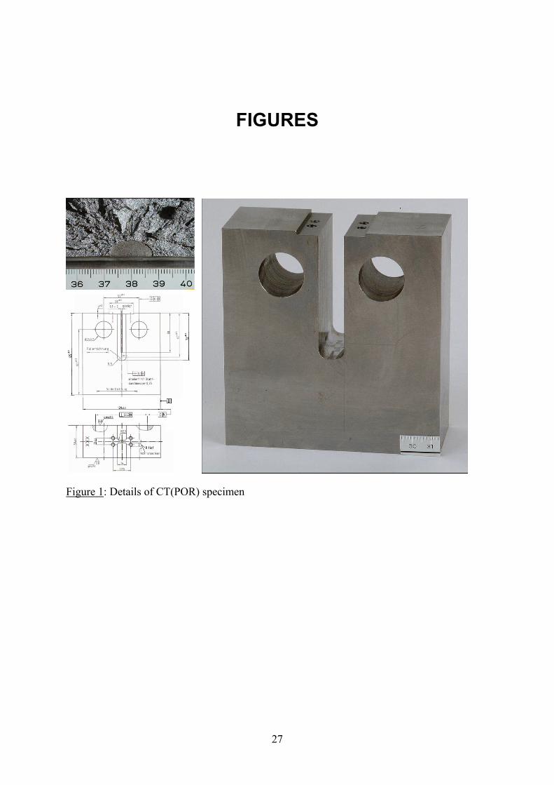
27

FIGURES

Figure 1: Details of CT(POR) specimen

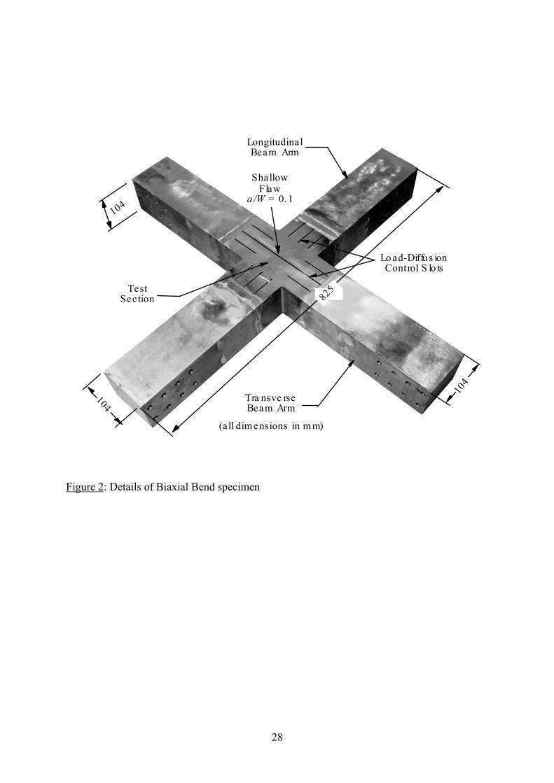
28

Figure 2: Details of Biaxial Bend specimen

825

104

104

Longitudinal Beam Arm

Tra nsve rse Beam Arm

Test Section

(all dim ensions in m m)

Lo ad-Diffu s ion Control S lo ts

Shallow Flaw

a /W = 0.1

104

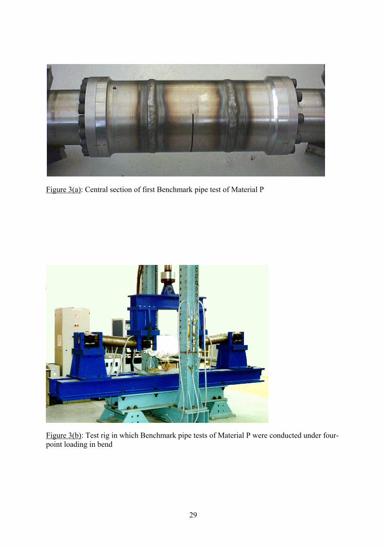
29

Figure 3(a): Central section of first Benchmark pipe test of Material P

Figure 3(b): Test rig in which Benchmark pipe tests of Material P were conducted under four-point loading in bend

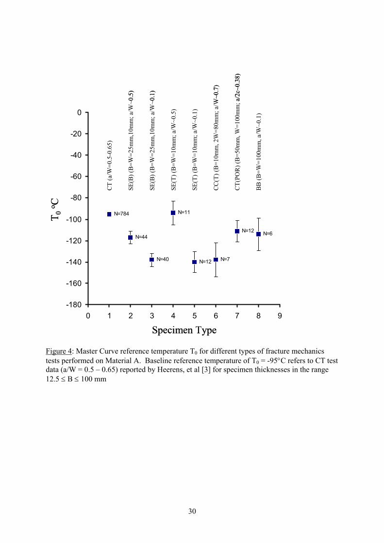
30

Figure 4: Master Curve reference temperature T0 for different types of fracture mechanics tests performed on Material A. Baseline reference temperature of T0 = -95°C refers to CT test data (a/W = 0.5 – 0.65) reported by Heerens, et al [3] for specimen thicknesses in the range 12.5 ≤ B ≤ 100 mm

N=44

N=40

N=11

N=12 N=7

N=12 N=6

N=784

-180

-160

-140

-120

-100

-80

-60

-40

-20

0

0 1 2 3 4 5 6 7 8 9

CT

(a/W

=0.5

-0.6

5)

SE(B

) (B

=W=2

5mm

,10m

m; a

/W~0

.5)

SE(B

) (B

=W=2

5mm

,10m

m; a

/W~0

.1)

SE(T

) (B

=W=1

0mm

; a/W

~0.5

)

SE(T

) (B

=W=1

0mm

; a/W

~0.1

)

CC

(T) (

B=1

0mm

, 2W

=80m

m; a

/W~0

.7)

CT(

POR

) (B

=50m

m, W

=100

mm

; a/2

c~0.

38)

BB

(B=W

=100

mm

, a/W

~0.1

)

T 0o C

Specimen Type

N=44

N=40

N=11

N=12 N=7

N=12 N=6

N=784

-180

-160

-140

-120

-100

-80

-60

-40

-20

0

0 1 2 3 4 5 6 7 8 9

CT

(a/W

=0.5

-0.6

5)

SE(B

) (B

=W=2

5mm

,10m

m; a

/W~0

.5)

SE(B

) (B

=W=2

5mm

,10m

m; a

/W~0

.1)

SE(T

) (B

=W=1

0mm

; a/W

~0.5

)

SE(T

) (B

=W=1

0mm

; a/W

~0.1

)

CC

(T) (

B=1

0mm

, 2W

=80m

m; a

/W~0

.7)

CT(

POR

) (B

=50m

m, W

=100

mm

; a/2

c~0.

38)

BB

(B=W

=100

mm

, a/W

~0.1

)

T 0o C

Specimen Type

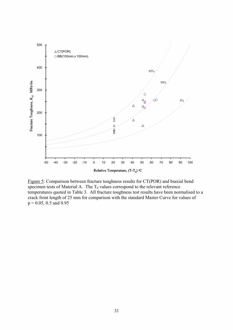
31

Figure 5: Comparison between fracture toughness results for CT(POR) and biaxial bend specimen tests of Material A. The T0 values correspond to the relevant reference temperatures quoted in Table 3. All fracture toughness test results have been normalised to a crack front length of 25 mm for comparison with the standard Master Curve for values of p = 0.05, 0.5 and 0.95

-

100

200

300

400

500

-50 -40 -30 -20 -10 0 10 20 30 40 50 60 70 80 90 100

CT(POR)BB(100mm x 100mm)

Relative Temperature, (T-T0) oC

Frac

ture

Tou

ghne

ss, K

JCM

Pa√m

5%

50%

95%

-

100

200

300

400

500

-50 -40 -30 -20 -10 0 10 20 30 40 50 60 70 80 90 100

CT(POR)BB(100mm x 100mm)

Relative Temperature, (T-T0) oC

Frac

ture

Tou

ghne

ss, K

JCM

Pa√m

5%

50%

95%

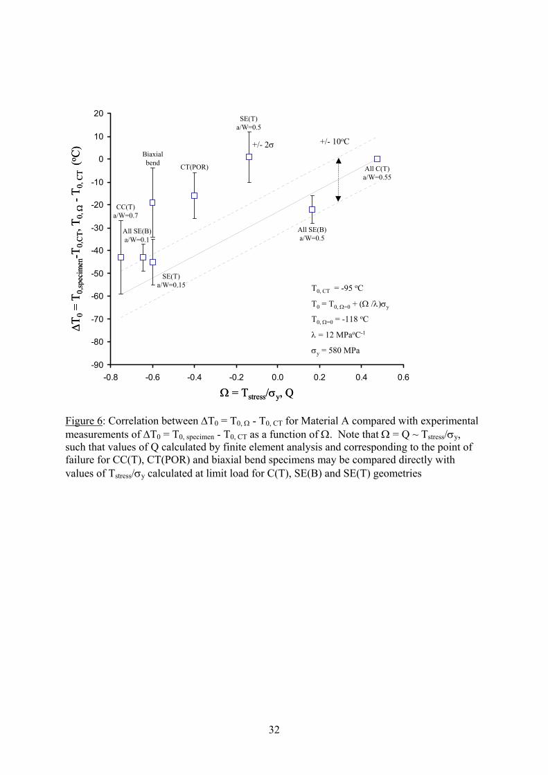
32

Figure 6: Correlation between ∆T0 = T0, Ω - T0, CT for Material A compared with experimental measurements of ∆T0 = T0, specimen - T0, CT as a function of Ω. Note that Ω = Q ~ Tstress/σy, such that values of Q calculated by finite element analysis and corresponding to the point of failure for CC(T), CT(POR) and biaxial bend specimens may be compared directly with values of Tstress/σy calculated at limit load for C(T), SE(B) and SE(T) geometries

-90

-80

-70

-60

-50

-40

-30

-20

-10

0

10

20

-0.8 -0.6 -0.4 -0.2 0.0 0.2 0.4 0.6

Ω = Tstress/σy, Q

All SE(B) a/W=0.5

All C(T) a/W=0.55

SE(T) a/W=0.5

CT(POR)

Biaxial bend

SE(T) a/W=0.15

All SE(B) a/W=0.1

CC(T) a/W=0.7

+/- 10oC+/- 2σ

∆T0

= T 0

,spec

imen

-T0,

CT,

T0,

Ω-T

0, C

T (o C

)

T0, CT = -95 oC

T0 = T0, Ω=0 + (Ω /λ)σy

T0, Ω=0 = -118 oC

λ = 12 MPaoC-1

σy = 580 MPa

-90

-80

-70

-60

-50

-40

-30

-20

-10

0

10

20

-0.8 -0.6 -0.4 -0.2 0.0 0.2 0.4 0.6

Ω = Tstress/σy, Q

All SE(B) a/W=0.5

All C(T) a/W=0.55

SE(T) a/W=0.5

CT(POR)

Biaxial bend

SE(T) a/W=0.15

All SE(B) a/W=0.1

CC(T) a/W=0.7

+/- 10oC+/- 2σ

∆T0

= T 0

,spec

imen

-T0,

CT,

T0,

Ω-T

0, C

T (o C

)

T0, CT = -95 oC

T0 = T0, Ω=0 + (Ω /λ)σy

T0, Ω=0 = -118 oC

λ = 12 MPaoC-1

σy = 580 MPa

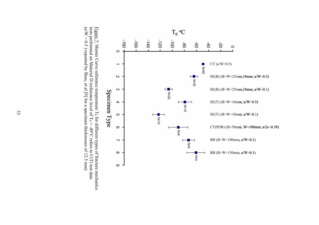
33

Figure 7: Master C

urve reference temperature T

0 for different types of fracture mechanics

tests performed on M

aterial D (reference level of T

0 = -49°C refers to C

(T) test data (a/W

= 0.5 ) reported by Bass, et al [9] for a specim

en thicknesses of 12.5 mm

)

N=30

N=26

N=12

N=12

N=8

N=6

N=4

N=60

-180

-160

-140

-120

-100

-80

-60

-40

-20 0

01

23

45

67

89

Specimen Type

T0oC

CT (a/W=0.5)

SE(B) (B=W=25mm,10mm; a/W~0.5)

SE(B) (B=W=25mm,10mm; a/W~0.1)

SE(T) (B=W=10mm; a/W~0.5)

SE(T) (B=W=10mm; a/W~0.1)

CT(POR) (B=50mm, W=100mm; a/2c~0.38)

BB (B=W=100mm, a/W~0.1)

BB (B=W=150mm, a/W~0.1)

N=30

N=26

N=12

N=12

N=8

N=6

N=4

N=60

-180

-160

-140

-120

-100

-80

-60

-40

-20 0

01

23

45

67

89

Specimen Type

T0oC

CT (a/W=0.5)

SE(B) (B=W=25mm,10mm; a/W~0.5)

SE(B) (B=W=25mm,10mm; a/W~0.1)

SE(T) (B=W=10mm; a/W~0.5)

SE(T) (B=W=10mm; a/W~0.1)

CT(POR) (B=50mm, W=100mm; a/2c~0.38)

BB (B=W=100mm, a/W~0.1)

BB (B=W=150mm, a/W~0.1)

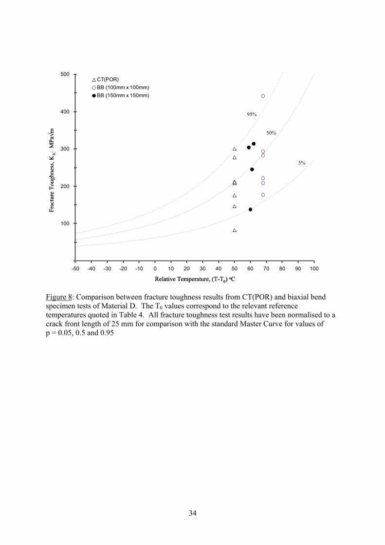
34

Figure 8: Comparison between fracture toughness results from CT(POR) and biaxial bend specimen tests of Material D. The T0 values correspond to the relevant reference temperatures quoted in Table 4. All fracture toughness test results have been normalised to a crack front length of 25 mm for comparison with the standard Master Curve for values of p = 0.05, 0.5 and 0.95

-

100

200

300

400

500

-50 -40 -30 -20 -10 0 10 20 30 40 50 60 70 80 90 100

CT(POR)BB (100mm x 100mm)BB (150mm x 150mm)

Frac

ture

Tou

ghne

ss, K

JCM

Pa√m

Relative Temperature, (T-T0) oC

5%

50%

95%

-

100

200

300

400

500

-50 -40 -30 -20 -10 0 10 20 30 40 50 60 70 80 90 100

CT(POR)BB (100mm x 100mm)BB (150mm x 150mm)

Frac

ture

Tou

ghne

ss, K

JCM

Pa√m

Relative Temperature, (T-T0) oC

5%

50%

95%

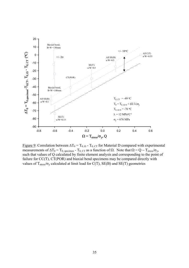
35

Figure 9: Correlation between ∆T0 = T0, Ω - T0, CT for Material D compared with experimental measurements of ∆T0 = T0, specimen - T0, CT as a function of Ω. Note that Ω = Q ~ Tstress/σy, such that values of Q calculated by finite element analysis and corresponding to the point of failure for CC(T), CT(POR) and biaxial bend specimens may be compared directly with values of Tstress/σy calculated at limit load for C(T), SE(B) and SE(T) geometries

-90

-80

-70

-60

-50

-40

-30

-20

-10

0

10

20

-0.8 -0.6 -0.4 -0.2 0.0 0.2 0.4 0.6

Ω = Tstress/σy, Q

+/- 10oC

+/- 2σAll C(T) a/W=0.55All SE(B)

a/W=0.5

SE(T) a/W=0.5

CT(POR)

Biaxial bend, B=W=150mm

Biaxial bend, B=W=100mm

All SE(B) a/W=0.1

SE(T) a/W=0.15

∆T 0

= T 0

,spec

imen

-T0,

CT,

T0,

Ω-T

0, C

T (o C

)

T0, CT = -49 oC

T0 = T0, Ω=0 + (Ω /λ)σy

T0, Ω=0 = -76 oC

λ = 12 MPaoC-1

σy = 676 MPa

-90

-80

-70

-60

-50

-40

-30

-20

-10

0

10

20

-0.8 -0.6 -0.4 -0.2 0.0 0.2 0.4 0.6

Ω = Tstress/σy, Q

+/- 10oC

+/- 2σAll C(T) a/W=0.55All SE(B)

a/W=0.5

SE(T) a/W=0.5

CT(POR)

Biaxial bend, B=W=150mm

Biaxial bend, B=W=100mm

All SE(B) a/W=0.1

SE(T) a/W=0.15

∆T 0

= T 0

,spec

imen

-T0,

CT,

T0,

Ω-T

0, C

T (o C

)

T0, CT = -49 oC

T0 = T0, Ω=0 + (Ω /λ)σy

T0, Ω=0 = -76 oC

λ = 12 MPaoC-1

σy = 676 MPa

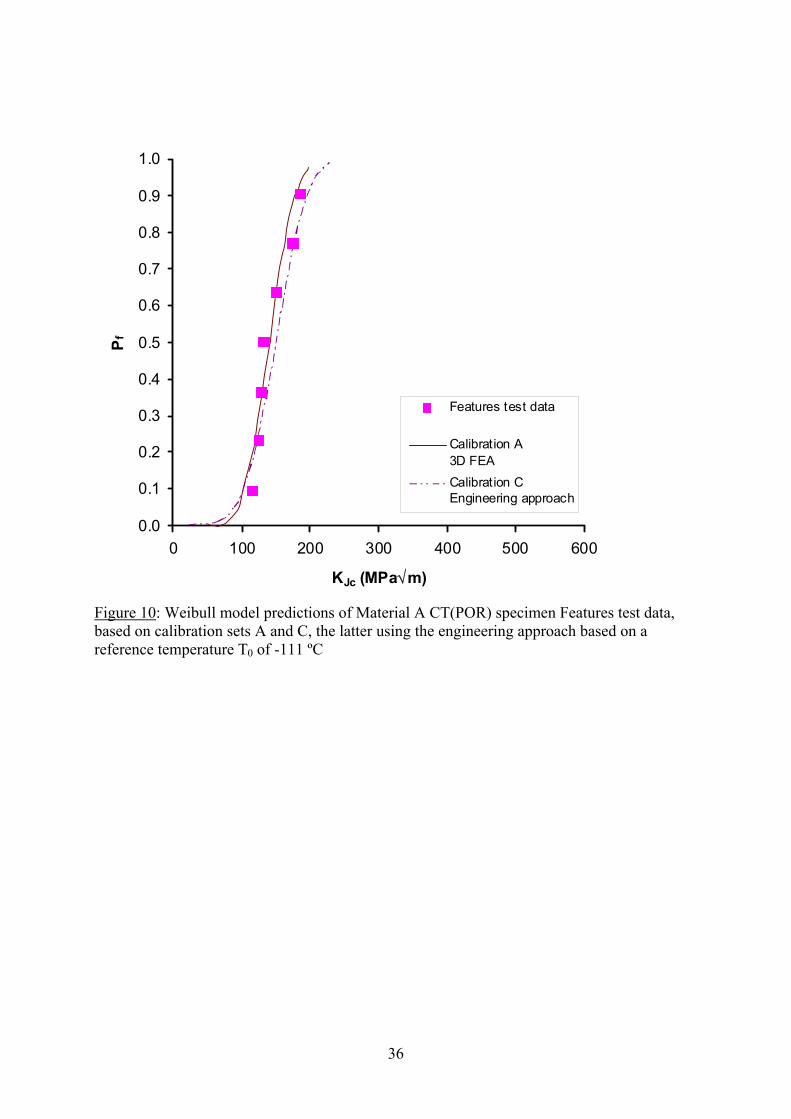
36

Figure 10: Weibull model predictions of Material A CT(POR) specimen Features test data, based on calibration sets A and C, the latter using the engineering approach based on a reference temperature T0 of -111 ºC

0.0

0.1

0.2

0.3

0.4

0.5

0.6

0.7

0.8

0.9

1.0

0 100 200 300 400 500 600

KJc (MPa√m)

Pf

Features test data

Calibration A3D FEACalibration CEngineering approach

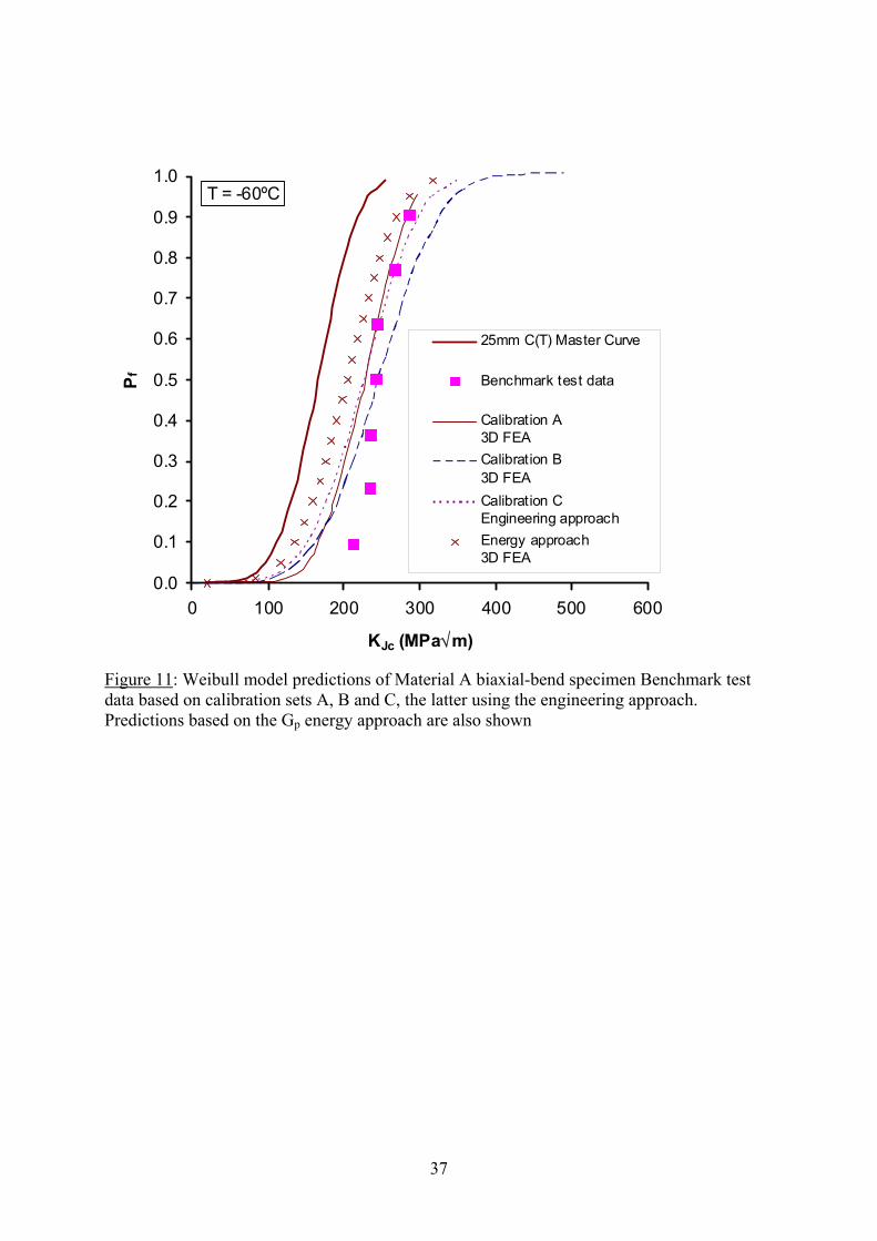
37

Figure 11: Weibull model predictions of Material A biaxial-bend specimen Benchmark test data based on calibration sets A, B and C, the latter using the engineering approach. Predictions based on the Gp energy approach are also shown

0.0

0.1

0.2

0.3

0.4

0.5

0.6

0.7

0.8

0.9

1.0

0 100 200 300 400 500 600

KJc (MPa√m)

Pf

25mm C(T) Master Curve

Benchmark test data

Calibration A3D FEACalibration B3D FEACalibration CEngineering approachEnergy approach3D FEA

T = -60ºC

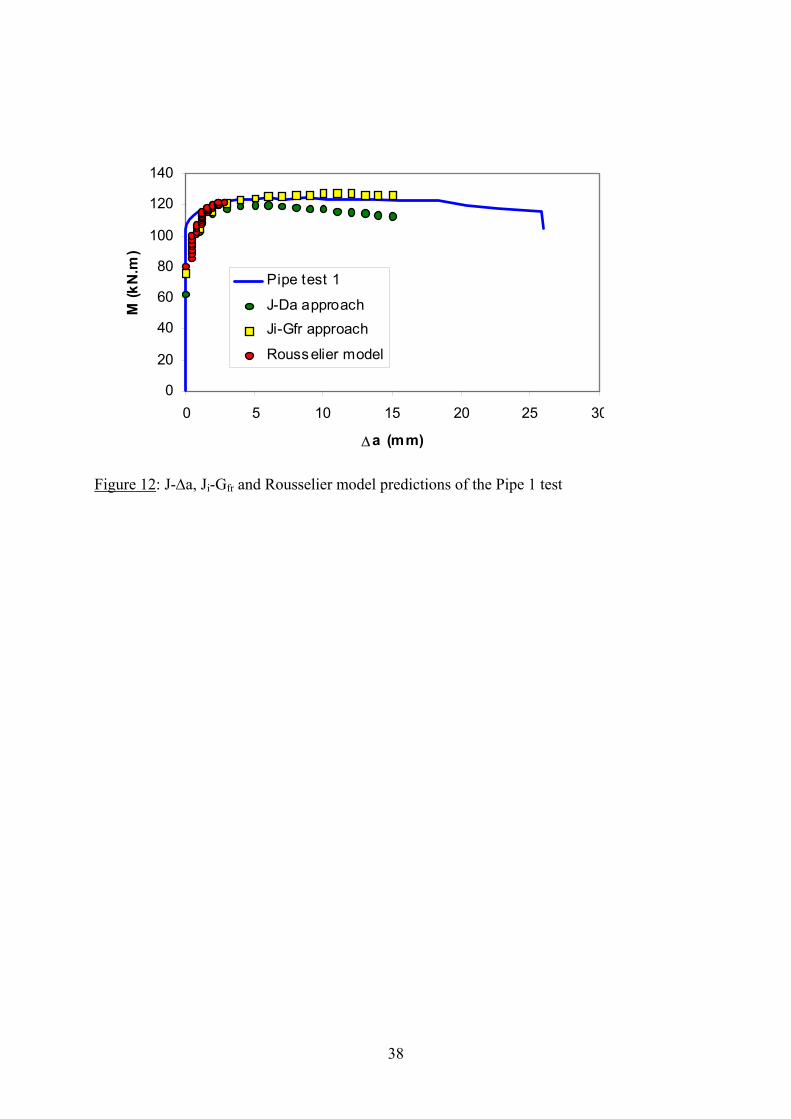
38

Figure 12: J-∆a, Ji-Gfr and Rousselier model predictions of the Pipe 1 test

0

20

40

60

80

100

120

140

0 5 10 15 20 25 30

∆a (mm)

M (k

N.m

)

Pipe test 1

J-Da approachJi-Gfr approach

Rousselier model

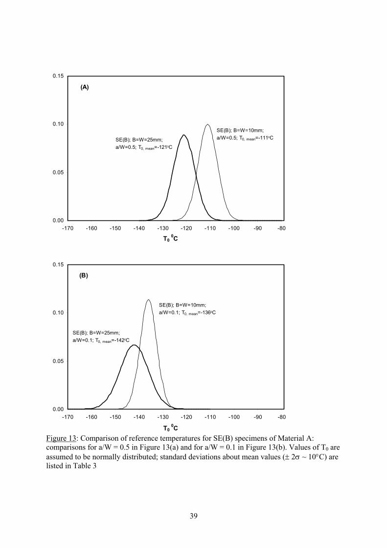
39

Figure 13: Comparison of reference temperatures for SE(B) specimens of Material A: comparisons for a/W = 0.5 in Figure 13(a) and for a/W = 0.1 in Figure 13(b). Values of T0 are assumed to be normally distributed; standard deviations about mean values (± 2σ ~ 10°C) are listed in Table 3

0.00

0.05

0.10

0.15

-170 -160 -150 -140 -130 -120 -110 -100 -90 -80

SE(B); B=W=25mm; a/W=0.5; T0, mean=-1210C

SE(B); B=W=10mm; a/W=0.5; T0, mean=-1110C

T0 0C

(A)

0.00

0.05

0.10

0.15

-170 -160 -150 -140 -130 -120 -110 -100 -90 -80

SE(B); B=W=25mm; a/W=0.1; T0, mean=-1420C

SE(B); B=W=10mm; a/W=0.1; T0, mean=-1360C

T0 0C

(B)

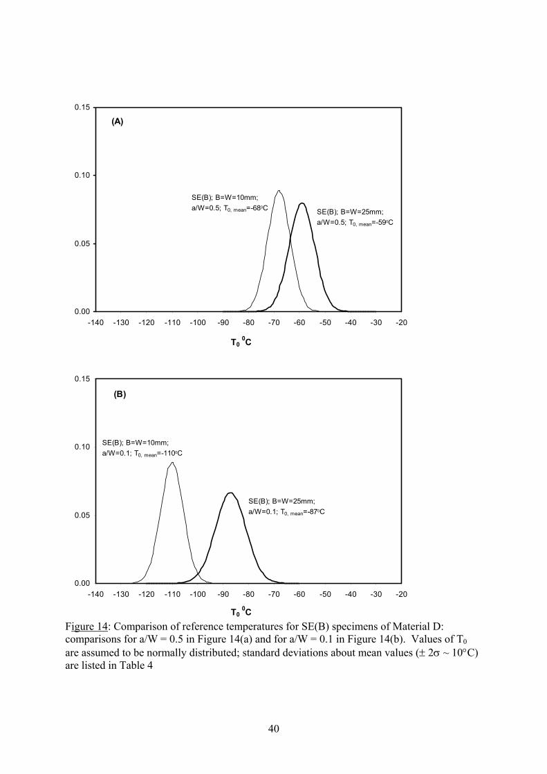
40

Figure 14: Comparison of reference temperatures for SE(B) specimens of Material D: comparisons for a/W = 0.5 in Figure 14(a) and for a/W = 0.1 in Figure 14(b). Values of T0 are assumed to be normally distributed; standard deviations about mean values (± 2σ ~ 10°C) are listed in Table 4

0.00

0.05

0.10

0.15

-140 -130 -120 -110 -100 -90 -80 -70 -60 -50 -40 -30 -20

SE(B); B=W=25mm; a/W=0.5; T0, mean=-590C

SE(B); B=W=10mm; a/W=0.5; T0, mean=-680C

T0 0C

(A)

0.00

0.05

0.10

0.15

-140 -130 -120 -110 -100 -90 -80 -70 -60 -50 -40 -30 -20

SE(B); B=W=10mm; a/W=0.1; T0, mean=-1100C

SE(B); B=W=25mm; a/W=0.1; T0, mean=-870C

T0 0C

(B)

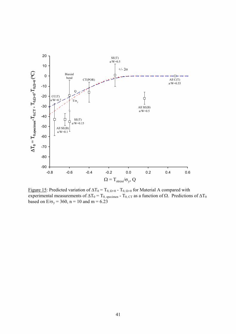
41

Figure 15: Predicted variation of ∆T0 = T0, Ω<0 - T0, Ω=0 for Material A compared with experimental measurements of ∆T0 = T0, specimen - T0, CT as a function of Ω. Predictions of ∆T0 based on E/σy = 360, n = 10 and m = 6.23

-90

-80

-70

-60

-50

-40

-30

-20

-10

0

10

20

-0.8 -0.6 -0.4 -0.2 0.0 0.2 0.4 0.6

Ω = Tstress/σy, Q

All SE(B) a/W=0.5

All C(T) a/W=0.55

SE(T) a/W=0.5

CT(POR)

Biaxial bend

SE(T) a/W=0.15

All SE(B) a/W=0.1

CC(T) a/W=0.7

∆T0

= T 0

,spec

imen

-T0,

CT

, T0,

Ω<0

-T0,

Ω=0

(o C) +/- 2σ

T/σy

Q

-90

-80

-70

-60

-50

-40

-30

-20

-10

0

10

20

-0.8 -0.6 -0.4 -0.2 0.0 0.2 0.4 0.6

Ω = Tstress/σy, Q

All SE(B) a/W=0.5

All C(T) a/W=0.55

SE(T) a/W=0.5

CT(POR)

Biaxial bend

SE(T) a/W=0.15

All SE(B) a/W=0.1

CC(T) a/W=0.7

∆T0

= T 0

,spec

imen

-T0,

CT

, T0,

Ω<0

-T0,

Ω=0

(o C) +/- 2σ

T/σy

Q

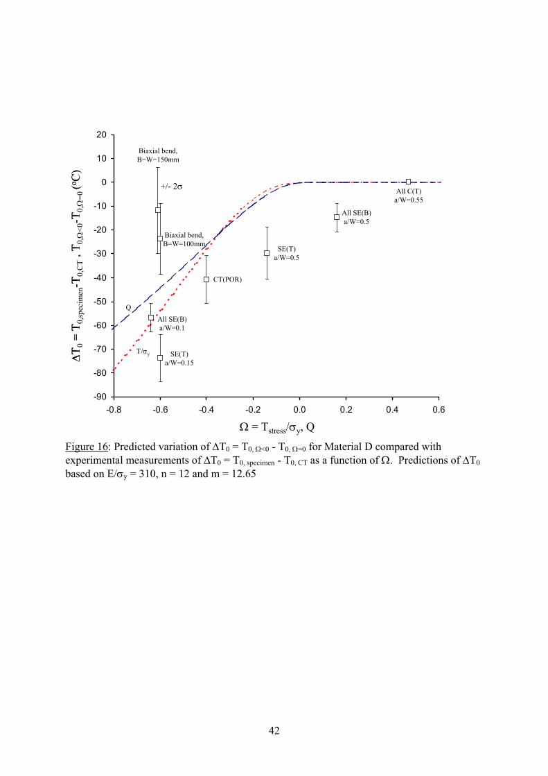
42

Figure 16: Predicted variation of ∆T0 = T0, Ω<0 - T0, Ω=0 for Material D compared with experimental measurements of ∆T0 = T0, specimen - T0, CT as a function of Ω. Predictions of ∆T0 based on E/σy = 310, n = 12 and m = 12.65

-90

-80

-70

-60

-50

-40

-30

-20

-10

0

10

20

-0.8 -0.6 -0.4 -0.2 0.0 0.2 0.4 0.6

Ω = Tstress/σy, Q

+/- 2σ All C(T) a/W=0.55

All SE(B) a/W=0.5

SE(T) a/W=0.5

CT(POR)

Biaxial bend, B=W=150mm

Biaxial bend, B=W=100mm

All SE(B) a/W=0.1

SE(T) a/W=0.15∆T

0=

T 0,sp

ecim

en-T

0,C

T, T

0,Ω

<0-T

0,Ω

=0 (o C

)

T/σy

Q

-90

-80

-70

-60

-50

-40

-30

-20

-10

0

10

20

-0.8 -0.6 -0.4 -0.2 0.0 0.2 0.4 0.6

Ω = Tstress/σy, Q

+/- 2σ All C(T) a/W=0.55

All SE(B) a/W=0.5

SE(T) a/W=0.5

CT(POR)

Biaxial bend, B=W=150mm

Biaxial bend, B=W=100mm

All SE(B) a/W=0.1

SE(T) a/W=0.15∆T

0=

T 0,sp

ecim

en-T

0,C

T, T

0,Ω

<0-T

0,Ω

=0 (o C

)

T/σy

Q

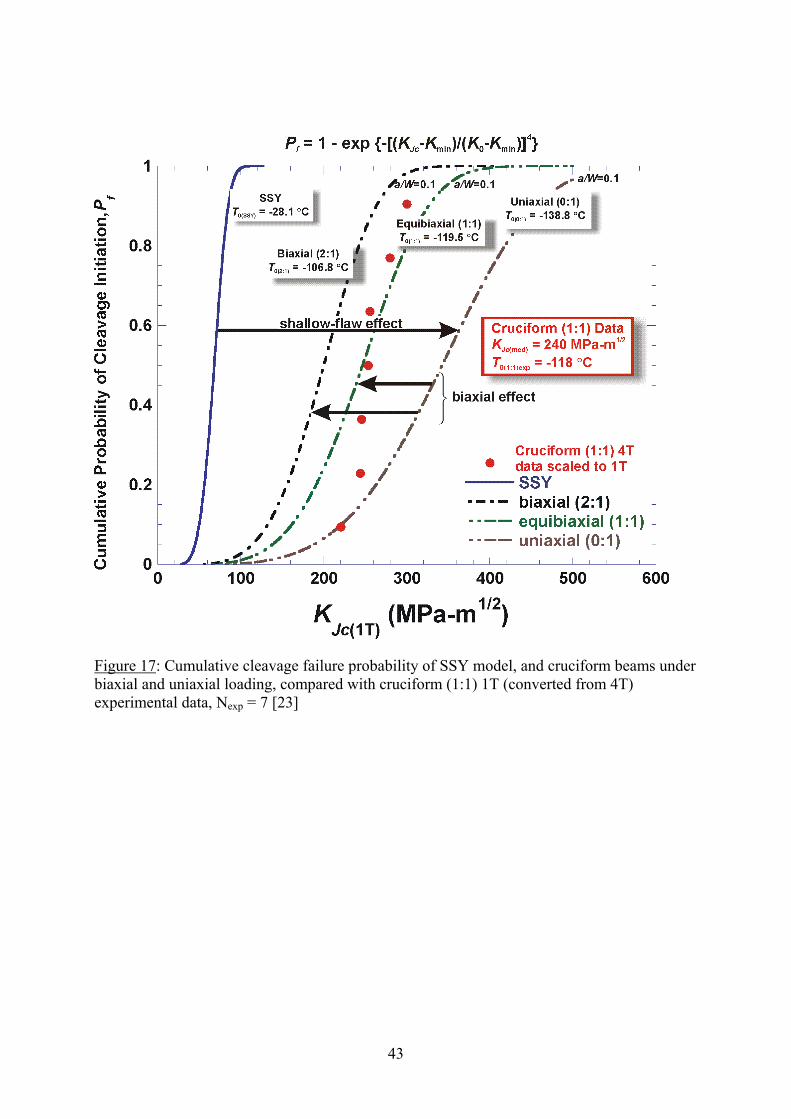
43

Figure 17: Cumulative cleavage failure probability of SSY model, and cruciform beams under biaxial and uniaxial loading, compared with cruciform (1:1) 1T (converted from 4T) experimental data, Nexp = 7 [23]

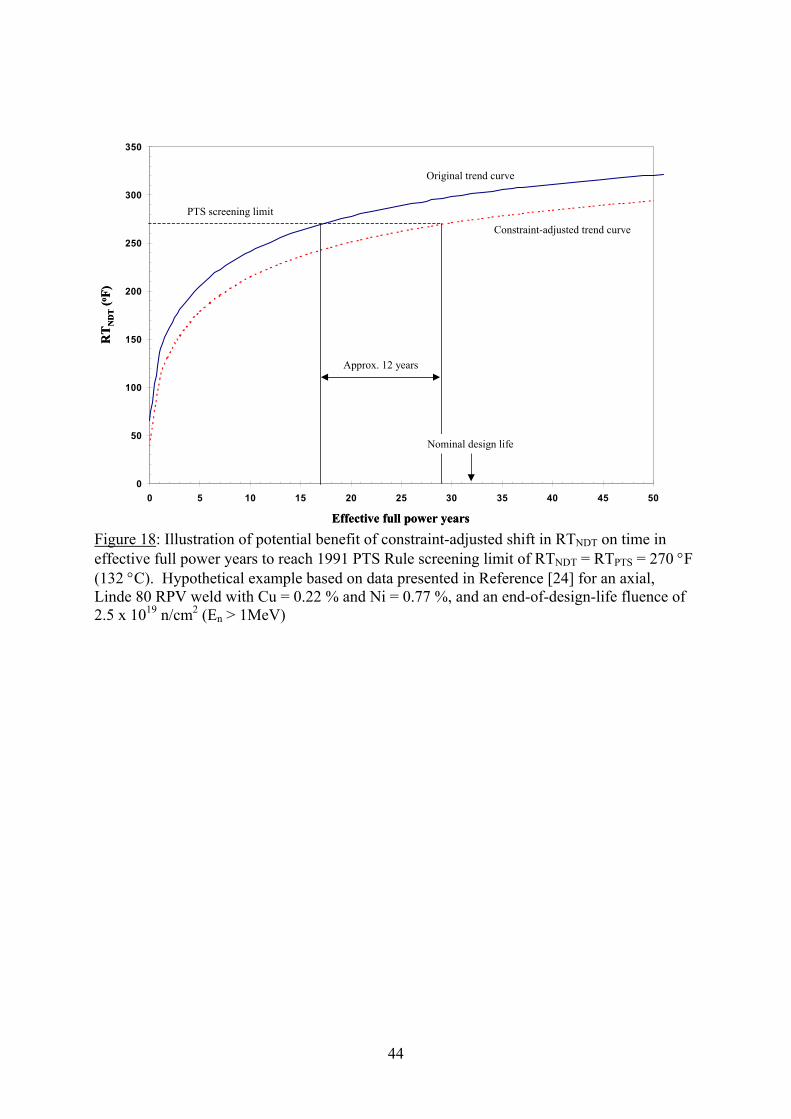
44

Figure 18: Illustration of potential benefit of constraint-adjusted shift in RTNDT on time in effective full power years to reach 1991 PTS Rule screening limit of RTNDT = RTPTS = 270 °F (132 °C). Hypothetical example based on data presented in Reference [24] for an axial, Linde 80 RPV weld with Cu = 0.22 % and Ni = 0.77 %, and an end-of-design-life fluence of 2.5 x 1019 n/cm2 (En > 1MeV)

0

50

100

150

200

250

300

350

0 5 10 15 20 25 30 35 40 45 50

Effective full power years

RT

ND

T(o F

)

Nominal design life

PTS screening limit

Constraint-adjusted trend curve

Original trend curve

Approx. 12 years

0

50

100

150

200

250

300

350

0 5 10 15 20 25 30 35 40 45 50

Effective full power years

RT

ND

T(o F

)

Nominal design life

PTS screening limit

Constraint-adjusted trend curve

Original trend curve

Approx. 12 years