NUMERICAL ANALYSIS OF SILO DISCHARGE - · PDF fileNUMERICAL ANALYSIS OF SILO DISCHARGE. ... To fulﬂll these two demands the original design of the silo has a perforated inner tube

Master’s DissertationStructural

Mechanics

JOHN BROWN

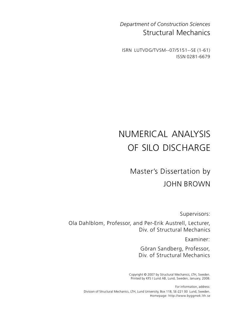
NUMERICAL ANALYSISOF SILO DISCHARGE

Denna sida skall vara tom!

Copyright © 2007 by Structural Mechanics, LTH, Sweden.Printed by KFS I Lund AB, Lund, Sweden, January, 2008.

For information, address:

Division of Structural Mechanics, LTH, Lund University, Box 118, SE-221 00 Lund, Sweden.Homepage: http://www.byggmek.lth.se

Structural MechanicsDepartment of Construction Sciences

Master’s Dissertation by

JOHN BROWN

Supervisors:

Ola Dahlblom, Professor, and Per-Erik Austrell, Lecturer,Div. of Structural Mechanics

NUMERICAL ANALYSIS

OF SILO DISCHARGE

ISRN LUTVDG/TVSM--07/5151--SE (1-61)ISSN 0281-6679

Examiner:

Göran Sandberg, Professor,Div. of Structural Mechanics


Abstract

A silo discharge with a bulk material consisting of iron ore pellets is studied. The silo isabout 65 meters high and 38 meters wide. The quality of pellets decreases when they areexposed to high stresses while moving. The stresses are therefore not allowed to exceeda certain threshold. It must also be possible to trace the origin of a sample from thedischarge. To fulfill these two demands the original design of the silo has a perforatedinner tube to obtain a specific flow pattern.

The simulations are performed using the finite element method with the pellets as a con-tinuum in three dimensions. The constitutive relation used for the pellets is the Drucker-Prager plasticity model. The simulations are performed with the commercial softwareABAQUS/Explicit and a pure Eulerian adaptive mesh. The preliminary original design issimulated together with proposed modified designs that benefit pellet quality.

The result of the original design exceeds the threshold stress level and lacks the possibilityto trace the sample’s origin. Of the investigated modified designs there is one that showslower stresses and improved traceability; a silo where the inner tube has a smaller radiusthan the original design.

Keywords: Granular flow, Silo, Iron ore pellets, Inner tube, FEM, ABAQUS.

i


Contents

Abstract i

I Introduction 1

1 Introduction 31.1 Objective . . . . . . . . . . . . . . . . . . . . . . . . . . . . . . . . . . . . . 41.2 Delimitations . . . . . . . . . . . . . . . . . . . . . . . . . . . . . . . . . . . 41.3 Disposition . . . . . . . . . . . . . . . . . . . . . . . . . . . . . . . . . . . . 4

2 Project presentation 52.1 Iron ore pellets . . . . . . . . . . . . . . . . . . . . . . . . . . . . . . . . . . 62.2 The silos . . . . . . . . . . . . . . . . . . . . . . . . . . . . . . . . . . . . . . 62.3 The thesis . . . . . . . . . . . . . . . . . . . . . . . . . . . . . . . . . . . . . 7

II Theory and methodology 11

3 Finite element formulation 133.1 Analysis type . . . . . . . . . . . . . . . . . . . . . . . . . . . . . . . . . . . 133.2 Stability and increment time . . . . . . . . . . . . . . . . . . . . . . . . . . 153.3 Adaptive mesh generation . . . . . . . . . . . . . . . . . . . . . . . . . . . . 15

3.3.1 Tracer particle . . . . . . . . . . . . . . . . . . . . . . . . . . . . . . 163.4 Quad element with reduced integration . . . . . . . . . . . . . . . . . . . . . 16

4 Constitutive relations 174.1 Mohr-Coulomb plasticity . . . . . . . . . . . . . . . . . . . . . . . . . . . . . 184.2 Drucker-Prager plasticity . . . . . . . . . . . . . . . . . . . . . . . . . . . . 194.3 Frictional contact . . . . . . . . . . . . . . . . . . . . . . . . . . . . . . . . . 20

5 Simulation conditions 215.1 Density . . . . . . . . . . . . . . . . . . . . . . . . . . . . . . . . . . . . . . 215.2 Elasticity . . . . . . . . . . . . . . . . . . . . . . . . . . . . . . . . . . . . . 215.3 Plasticity . . . . . . . . . . . . . . . . . . . . . . . . . . . . . . . . . . . . . 225.4 Friction . . . . . . . . . . . . . . . . . . . . . . . . . . . . . . . . . . . . . . 225.5 Boundaries . . . . . . . . . . . . . . . . . . . . . . . . . . . . . . . . . . . . 235.6 Stresses and strain . . . . . . . . . . . . . . . . . . . . . . . . . . . . . . . . 24

iii

iv CONTENTS

III Result 25

6 Original design 276.1 Discharge state 1 . . . . . . . . . . . . . . . . . . . . . . . . . . . . . . . . . 28

6.1.1 Impact of the friction coefficient µ . . . . . . . . . . . . . . . . . . . 306.1.2 Impact of the material parameter β . . . . . . . . . . . . . . . . . . 32

6.2 Discharge state 2 . . . . . . . . . . . . . . . . . . . . . . . . . . . . . . . . . 346.3 Discharge state 3 . . . . . . . . . . . . . . . . . . . . . . . . . . . . . . . . . 34

7 Modified design 377.1 No inner tube . . . . . . . . . . . . . . . . . . . . . . . . . . . . . . . . . . . 387.2 Design modification 1 - Oblique plateau . . . . . . . . . . . . . . . . . . . . 407.3 Design modification 2 - Increased inclination in the hopper . . . . . . . . . 407.4 Design modification 3 - Varying thickness of the inner tube . . . . . . . . . 447.5 Design modification 4 - Shorter inner tube . . . . . . . . . . . . . . . . . . . 467.6 Design modification 5 - Decreased radius of the inner tube . . . . . . . . . . 48

IV Summary 51

8 Summary 538.1 Conclusions . . . . . . . . . . . . . . . . . . . . . . . . . . . . . . . . . . . . 548.2 Discussion . . . . . . . . . . . . . . . . . . . . . . . . . . . . . . . . . . . . . 548.3 Future work . . . . . . . . . . . . . . . . . . . . . . . . . . . . . . . . . . . . 55

References 57

A - Original drawings 61

Part I

Introduction

1

Chapter 1

Introduction

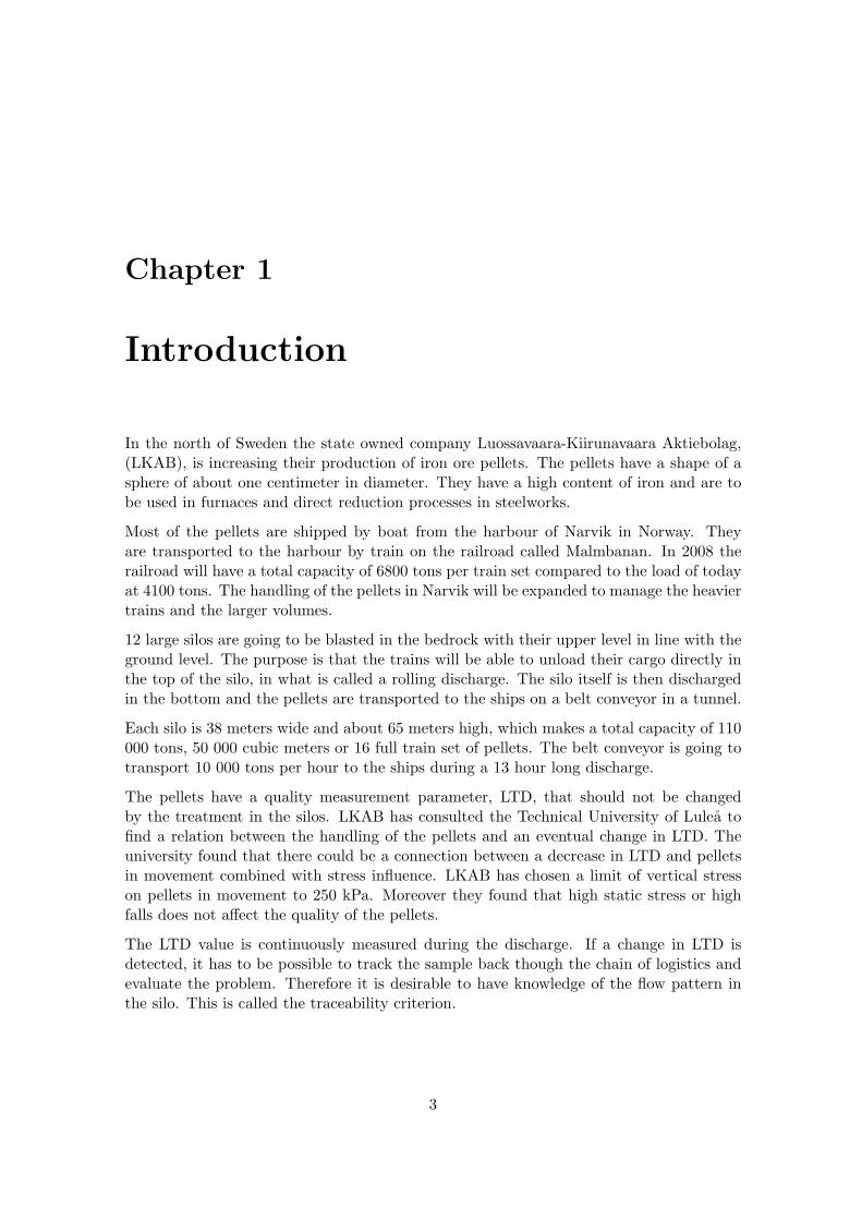
In the north of Sweden the state owned company Luossavaara-Kiirunavaara Aktiebolag,(LKAB), is increasing their production of iron ore pellets. The pellets have a shape of asphere of about one centimeter in diameter. They have a high content of iron and are tobe used in furnaces and direct reduction processes in steelworks.

Most of the pellets are shipped by boat from the harbour of Narvik in Norway. Theyare transported to the harbour by train on the railroad called Malmbanan. In 2008 therailroad will have a total capacity of 6800 tons per train set compared to the load of todayat 4100 tons. The handling of the pellets in Narvik will be expanded to manage the heaviertrains and the larger volumes.

12 large silos are going to be blasted in the bedrock with their upper level in line with theground level. The purpose is that the trains will be able to unload their cargo directly inthe top of the silo, in what is called a rolling discharge. The silo itself is then dischargedin the bottom and the pellets are transported to the ships on a belt conveyor in a tunnel.

Each silo is 38 meters wide and about 65 meters high, which makes a total capacity of 110000 tons, 50 000 cubic meters or 16 full train set of pellets. The belt conveyor is going totransport 10 000 tons per hour to the ships during a 13 hour long discharge.

The pellets have a quality measurement parameter, LTD, that should not be changedby the treatment in the silos. LKAB has consulted the Technical University of Lule̊a tofind a relation between the handling of the pellets and an eventual change in LTD. Theuniversity found that there could be a connection between a decrease in LTD and pelletsin movement combined with stress influence. LKAB has chosen a limit of vertical stresson pellets in movement to 250 kPa. Moreover they found that high static stress or highfalls does not affect the quality of the pellets.

The LTD value is continuously measured during the discharge. If a change in LTD isdetected, it has to be possible to track the sample back though the chain of logistics andevaluate the problem. Therefore it is desirable to have knowledge of the flow pattern inthe silo. This is called the traceability criterion.

3

4 CHAPTER 1. INTRODUCTION

1.1 Objective

There are two objectives in this thesis; the first is to determine the stresses in the pelletsand the second is to prove that the silo fulfills the traceability criterion. Both of themduring discharge.

Simulating the discharge of a silo will determine the stresses and compare this to a thresh-old value. If the stresses exceed these values, or if the traceability criterion fails, differentmodifications will be analyzed to find a better solution. The modifications will mainly begeometrical changes.

The work will be performed using the commercial finite element software ABAQUS.

1.2 Delimitations

The stresses in the silo will be compared with the stated value of 250 kPa vertical stressdetermined by LKAB. A more detailed investigation of the stresses inside the individualpellet or what is causing the decreasing quality are not processed.

There is a possibility to discuss different types of stress in the criterion because of uncer-tainties in the expression vertical stress.

Concerning the traceability criterion for the silo there is no delimitation.

All simulations assume that the pellets are filled symmetrically into the silo. No asym-metric load will therefore be investigated.

1.3 Disposition

The disposition is divided into four parts. First there is a presentation of the project andits background. The second part presents the theory together with the methodology thatare used in the simulations.

The results from the simulations are then presented in the third part, The Result, whichis divided into two chapters, the first investigates the original design at different statesand the second chapter that investigates different modified designs.

The fourth and last part is a summary of the entire work.

Chapter 2

Project presentation

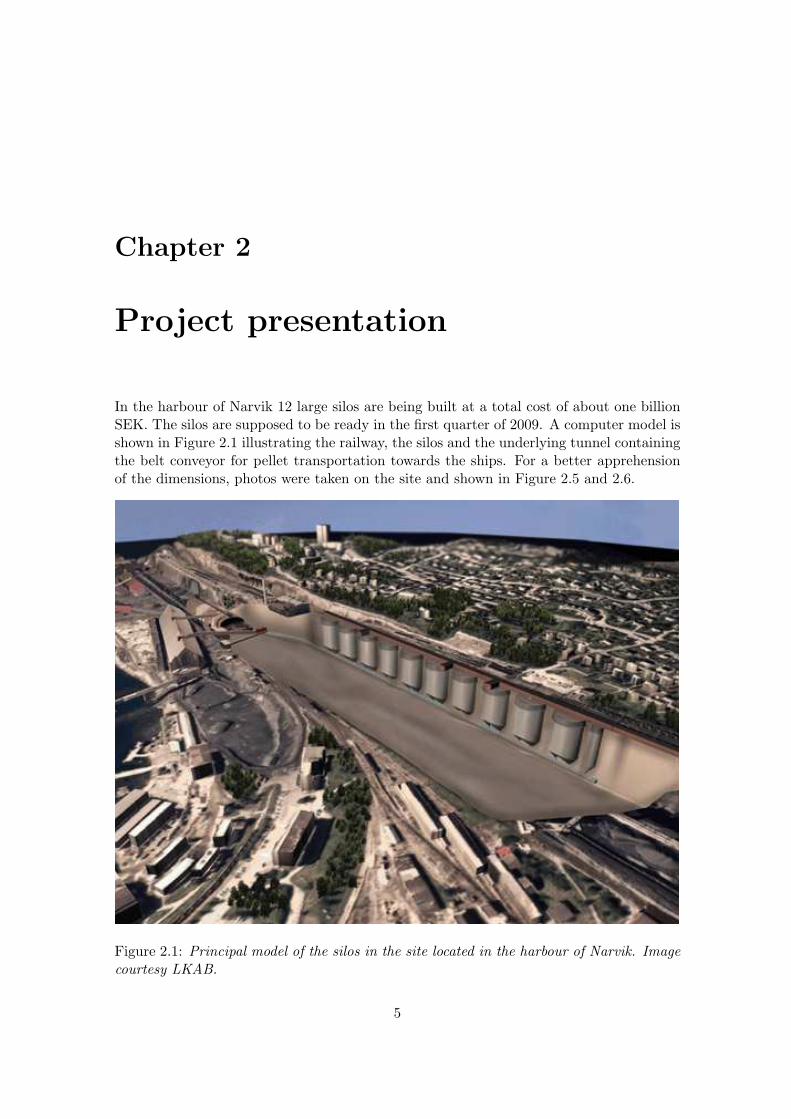
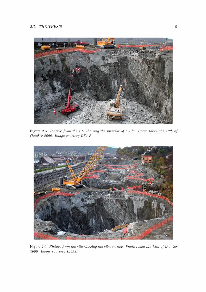
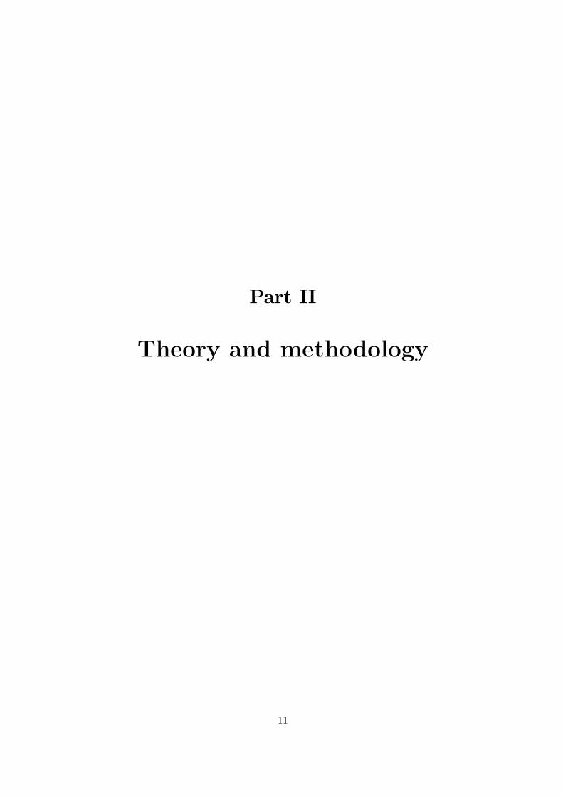
In the harbour of Narvik 12 large silos are being built at a total cost of about one billionSEK. The silos are supposed to be ready in the first quarter of 2009. A computer model isshown in Figure 2.1 illustrating the railway, the silos and the underlying tunnel containingthe belt conveyor for pellet transportation towards the ships. For a better apprehensionof the dimensions, photos were taken on the site and shown in Figure 2.5 and 2.6.

Figure 2.1: Principal model of the silos in the site located in the harbour of Narvik. Imagecourtesy LKAB.

5

6 CHAPTER 2. PROJECT PRESENTATION

2.1 Iron ore pellets

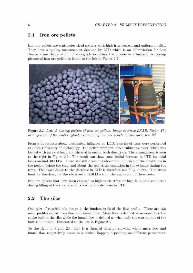
Iron ore pellets are centimeter sized spheres with high iron content and uniform quality.They have a quality measurement denoted by LTD which is an abbreviation for LowTemperature Degradation. The degradation refers the process in a furnace. A closeuppicture of iron ore pellets is found to the left in Figure 2.2

Figure 2.2: Left: A closeup picture of iron ore pellets. Image courtesy LKAB. Right: Thearrangement of the rubber cylinder containing iron ore pellets during shear test [6].

From a hypothesis about mechanical influence on LTD, a series of tests were performedat Lule̊a University of Technology. The pellets were put into a rubber cylinder, which wasloaded with an axial load, and sheared in one or both directions. The arrangement is seento the right in Figure 2.2. The result can show some initial decrease in LTD for axialloads around 400 kPa. There are still questions about the influence of the conditions inthe pellets before the tests and about the real stress condition in the cylinder during thetests. The exact cause to the decrease in LTD is therefore not fully known. The stresslimit for the design of the silo is set to 250 kPa from the evaluation of these tests.

Iron ore pellets that have been exposed to high static stress or high falls, that can occurduring filling of the silos, are not showing any decrease in LTD.

2.2 The silos

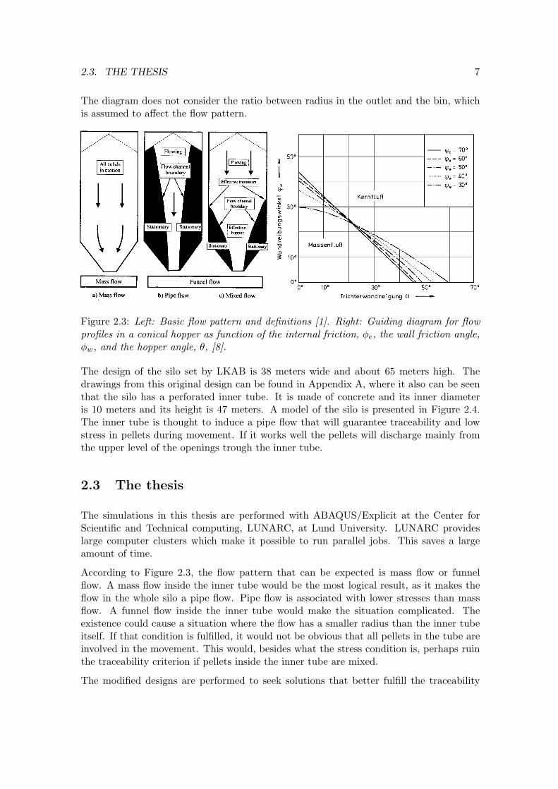
One part of classical silo design is the fundamentals of the flow profile. There are twomain profiles called mass flow and funnel flow. Mass flow is defined as movement of theentire bulk in the silo, while the funnel flow is defined as when only the central part of thebulk is in motion. Illustrated to the left in Figure 2.3.

To the right in Figure 2.3 there is a classical diagram showing where mass flow andfunnel flow respectively occur in a conical hopper, depending on different parameters.

2.3. THE THESIS 7

The diagram does not consider the ratio between radius in the outlet and the bin, whichis assumed to affect the flow pattern.

Figure 2.3: Left: Basic flow pattern and definitions [1]. Right: Guiding diagram for flowprofiles in a conical hopper as function of the internal friction, φe, the wall friction angle,φw, and the hopper angle, θ, [8].

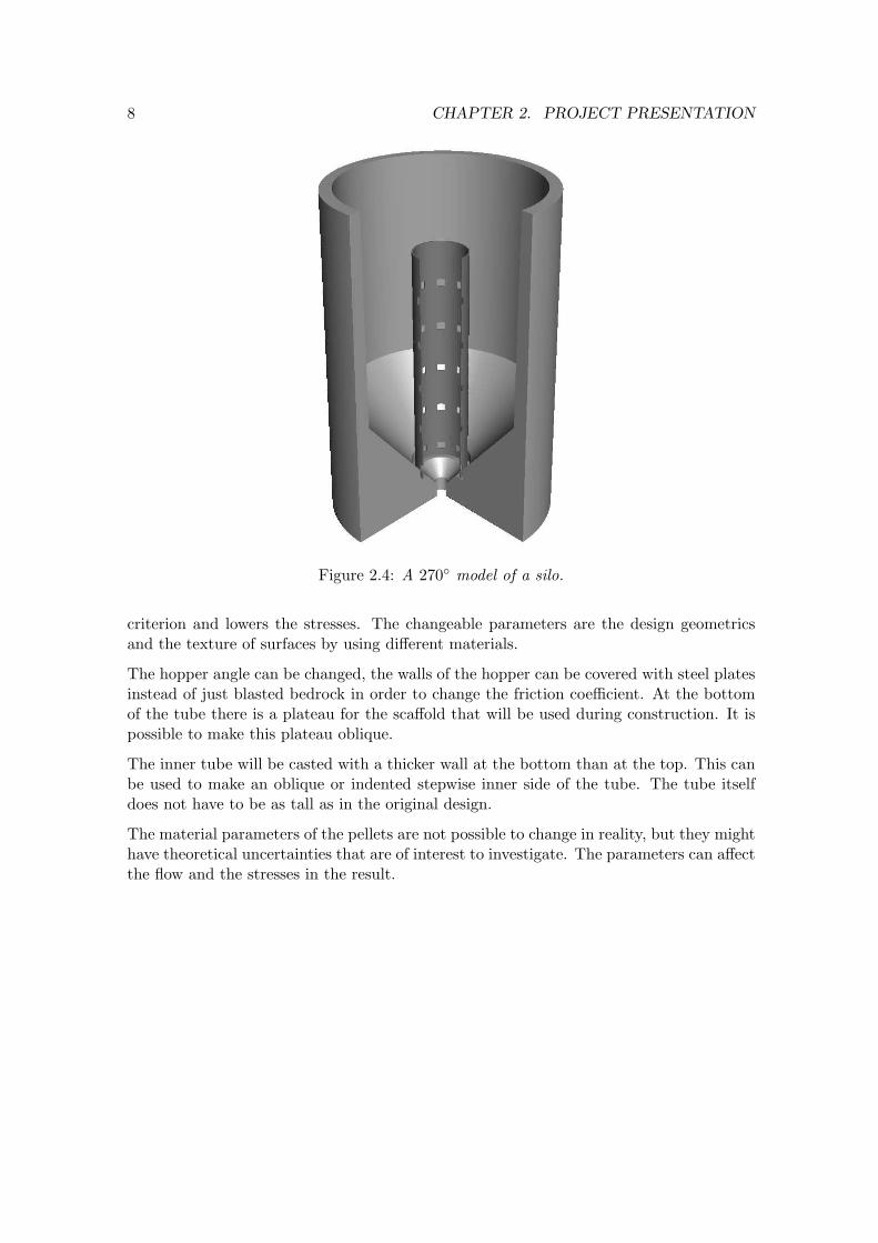
The design of the silo set by LKAB is 38 meters wide and about 65 meters high. Thedrawings from this original design can be found in Appendix A, where it also can be seenthat the silo has a perforated inner tube. It is made of concrete and its inner diameteris 10 meters and its height is 47 meters. A model of the silo is presented in Figure 2.4.The inner tube is thought to induce a pipe flow that will guarantee traceability and lowstress in pellets during movement. If it works well the pellets will discharge mainly fromthe upper level of the openings trough the inner tube.

2.3 The thesis

The simulations in this thesis are performed with ABAQUS/Explicit at the Center forScientific and Technical computing, LUNARC, at Lund University. LUNARC provideslarge computer clusters which make it possible to run parallel jobs. This saves a largeamount of time.

According to Figure 2.3, the flow pattern that can be expected is mass flow or funnelflow. A mass flow inside the inner tube would be the most logical result, as it makes theflow in the whole silo a pipe flow. Pipe flow is associated with lower stresses than massflow. A funnel flow inside the inner tube would make the situation complicated. Theexistence could cause a situation where the flow has a smaller radius than the inner tubeitself. If that condition is fulfilled, it would not be obvious that all pellets in the tube areinvolved in the movement. This would, besides what the stress condition is, perhaps ruinthe traceability criterion if pellets inside the inner tube are mixed.

The modified designs are performed to seek solutions that better fulfill the traceability

8 CHAPTER 2. PROJECT PRESENTATION

Figure 2.4: A 270◦ model of a silo.

criterion and lowers the stresses. The changeable parameters are the design geometricsand the texture of surfaces by using different materials.

The hopper angle can be changed, the walls of the hopper can be covered with steel platesinstead of just blasted bedrock in order to change the friction coefficient. At the bottomof the tube there is a plateau for the scaffold that will be used during construction. It ispossible to make this plateau oblique.

The inner tube will be casted with a thicker wall at the bottom than at the top. This canbe used to make an oblique or indented stepwise inner side of the tube. The tube itselfdoes not have to be as tall as in the original design.

The material parameters of the pellets are not possible to change in reality, but they mighthave theoretical uncertainties that are of interest to investigate. The parameters can affectthe flow and the stresses in the result.

2.3. THE THESIS 9

Figure 2.5: Picture from the site showing the interior of a silo. Photo taken the 13th ofOctober 2006. Image courtesy LKAB.

Figure 2.6: Picture from the site showing the silos in row. Photo taken the 13th of October2006. Image courtesy LKAB.


Part II

Theory and methodology

11

Chapter 3

Finite element formulation

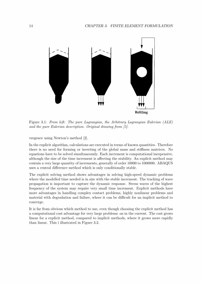
Finite element analysis are Lagrangian, which means that the mesh follows the materialin its movement. If the material has a movement that is comparable to a flow, butwithout for that sake being a pure fluid like in a silo with granular matter, it will havelarge deformations and the mesh will suffer of severe distortion. This can be handledby an adaptivity mesh technique, which recalculates and optimizes the mesh by certaincriterions during the analysis.

In a silo the Lagrangian description is suitable in the bin and at the upper free surface.At the outflow, where the material leaves the silo, the Eulerian is more suitable becausethen material can leave the mesh. The Eulerian description has a mesh that is fixed inspace. This calls for an Arbitrary Lagrangian Eulerian, ALE, description of the problemwhere the two types of analysis can be combined.

If the silo has inserts, which the flow has to pass, the Lagrangian description of the meshinside the bin will then again suffer from difficulties. As the upper surface of the materialmoves downwards, the mesh will be compressed above the insert. The only availablesolution is then the pure Eulerian description with the disadvantage that it must have afixed upper surface with an inflow, to make sure no element lacks material. Hence, onlysteady states can be evaluated.

An illustration of the pure Lagrangian, the Arbitrary Lagrangian Eulerian (ALE) and thepure Eulerian description is available in Figure 3.1.

3.1 Analysis type

There are two different algorithms to solve a dynamic finite element problem, implicit andexplicit. The implicit algorithm solves the equations of motion through the sets of coupleddifferential equations, in the mass and stiffness matrices, simultaneously. It is usuallyunconditionally stable and has no time increment size limit. However it is computationalexpensive to invert matrices and it may require many iterations to converge.

The implicit algorithm in ABAQUS uses the Hilber-Hughes-Taylor operator for integra-tion, which is an extension of the trapezoidal rule. The solution is then iterated to con-

13

14 CHAPTER 3. FINITE ELEMENT FORMULATION

Figure 3.1: From left: The pure Lagrangian, the Arbitrary Lagrangian Eulerian (ALE)and the pure Eulerian description. Original drawing from [5].

vergence using Newton’s method [2].

In the explicit algorithm, calculations are executed in terms of known quantities. Thereforethere is no need for forming or inverting of the global mass and stiffness matrices. Noequations have to be solved simultaneously. Each increment is computational inexpensive,although the size of the time increment is affecting the stability. An explicit method maycontain a very large quantity of increments, generally of order 10000 to 1000000. ABAQUSuses a central difference method which is only conditionally stable.

The explicit solving method shows advantages in solving high-speed dynamic problemswhere the modelled time needed is in size with the stable increment. The tracking of wavepropagation is important to capture the dynamic response. Stress waves of the highestfrequency of the system may require very small time increment. Explicit methods havemore advantages in handling complex contact problems, highly nonlinear problems andmaterial with degradation and failure, where it can be difficult for an implicit method toconverge.

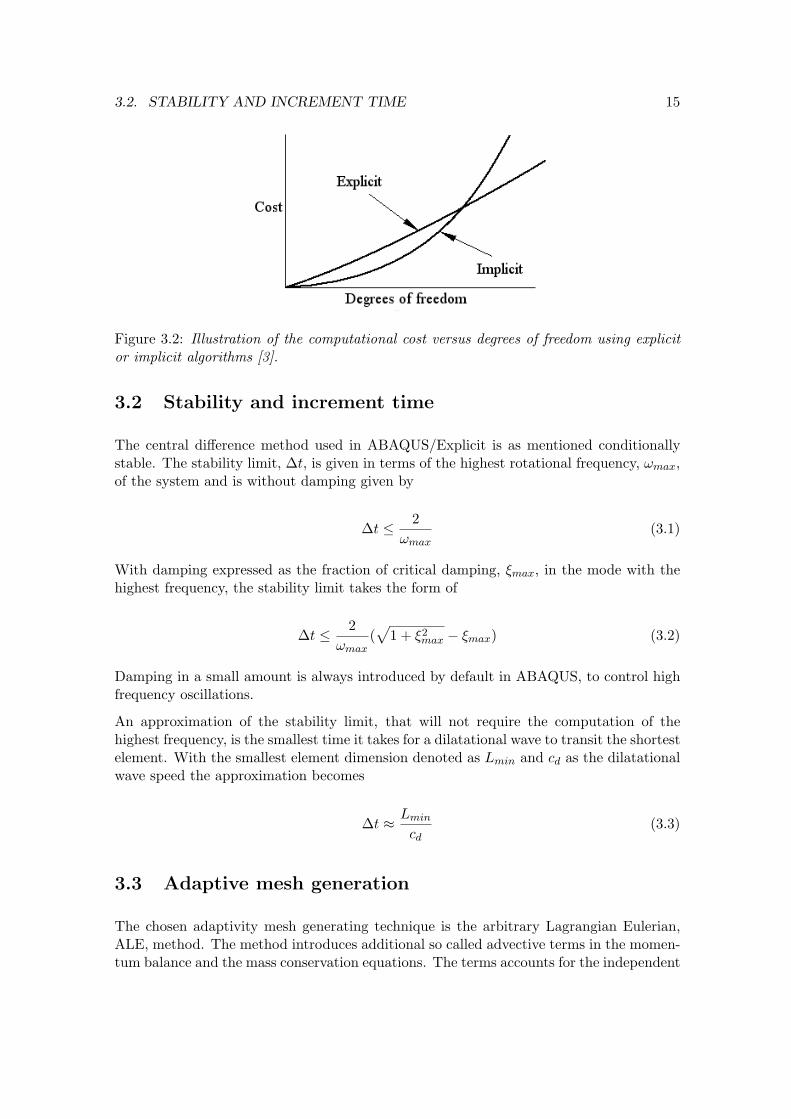
It is far from obvious which method to use, even though choosing the explicit method hasa computational cost advantage for very large problems -as in the current. The cost growslinear for a explicit method, compared to implicit methods, where it grows more rapidlythan linear. This i illustrated in Figure 3.2.

3.2. STABILITY AND INCREMENT TIME 15

Figure 3.2: Illustration of the computational cost versus degrees of freedom using explicitor implicit algorithms [3].

3.2 Stability and increment time

The central difference method used in ABAQUS/Explicit is as mentioned conditionallystable. The stability limit, ∆t, is given in terms of the highest rotational frequency, ωmax,of the system and is without damping given by

∆t ≤ 2ωmax

(3.1)

With damping expressed as the fraction of critical damping, ξmax, in the mode with thehighest frequency, the stability limit takes the form of

∆t ≤ 2ωmax

(√

1 + ξ2max − ξmax) (3.2)

Damping in a small amount is always introduced by default in ABAQUS, to control highfrequency oscillations.

An approximation of the stability limit, that will not require the computation of thehighest frequency, is the smallest time it takes for a dilatational wave to transit the shortestelement. With the smallest element dimension denoted as Lmin and cd as the dilatationalwave speed the approximation becomes

∆t ≈ Lmin

cd(3.3)

3.3 Adaptive mesh generation

The chosen adaptivity mesh generating technique is the arbitrary Lagrangian Eulerian,ALE, method. The method introduces additional so called advective terms in the momen-tum balance and the mass conservation equations. The terms accounts for the independent

16 CHAPTER 3. FINITE ELEMENT FORMULATION

mesh and material motion where the modified equations can be solved directly or by anoperator split that decouples the material motion from the additional mesh motion. Theoperator split is used in ABAQUS/Explicit since it is computationally efficient [2].

In every adaptive increment the whole model is first handled in a pure lagrangian manner.The solution is then remapped to the new mesh which is preformed by mesh sweeps undercertain criterions.

3.3.1 Tracer particle

There is a possibility to track the time history of specific nodes during the simulations bythe tracer particle function in ABAQUS. Every time an adaptivity increment is remappingthe mesh, it calculates the new position of an earlier defined node that completely followsthe physical matter.

The tracer particle can show movement, that is separated from vibrations, which aredifficult to observe in an Eulerian simulation where the mesh is fixed in space.

3.4 Quad element with reduced integration

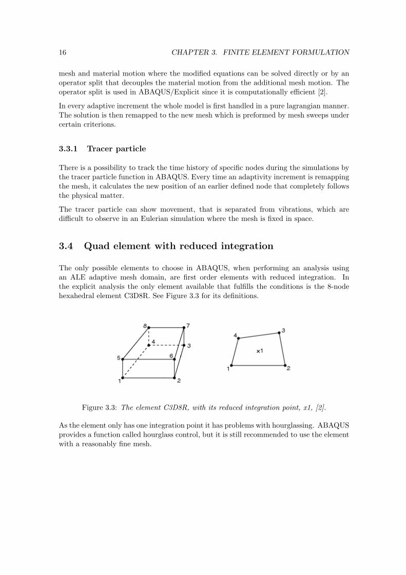
The only possible elements to choose in ABAQUS, when performing an analysis usingan ALE adaptive mesh domain, are first order elements with reduced integration. Inthe explicit analysis the only element available that fulfills the conditions is the 8-nodehexahedral element C3D8R. See Figure 3.3 for its definitions.

Figure 3.3: The element C3D8R, with its reduced integration point, x1, [2].

As the element only has one integration point it has problems with hourglassing. ABAQUSprovides a function called hourglass control, but it is still recommended to use the elementwith a reasonably fine mesh.

Chapter 4

Constitutive relations

Granular matter, as iron ore pellets, has a constitutive relation that depends on the normalstress to a specific surface, and will without cohesion not resist any tensile stress. At acertain state of stress the material will yield. The material will undergo deformations untilthe stress state is beneath the yield criterion, also called the failure model.

Granular material usually consolidates when exposed to long time stress. The bulk densityand shear strength increases as the particles become more tightly packed. When thematerial is exposed to deformation it will dilate, causing changes in the bulk density.Previous work of Karlsson [5] made the assumption that granular matter has constantbulk density as long as it is in motion.

In the simulation of flowing granular matter the initial consolidation is not taken intoaccount. Therefore the bulk density can be taken as constant. The material is non-dilatant, and iron ore pellets have no cohesion.

17

18 CHAPTER 4. CONSTITUTIVE RELATIONS

4.1 Mohr-Coulomb plasticity

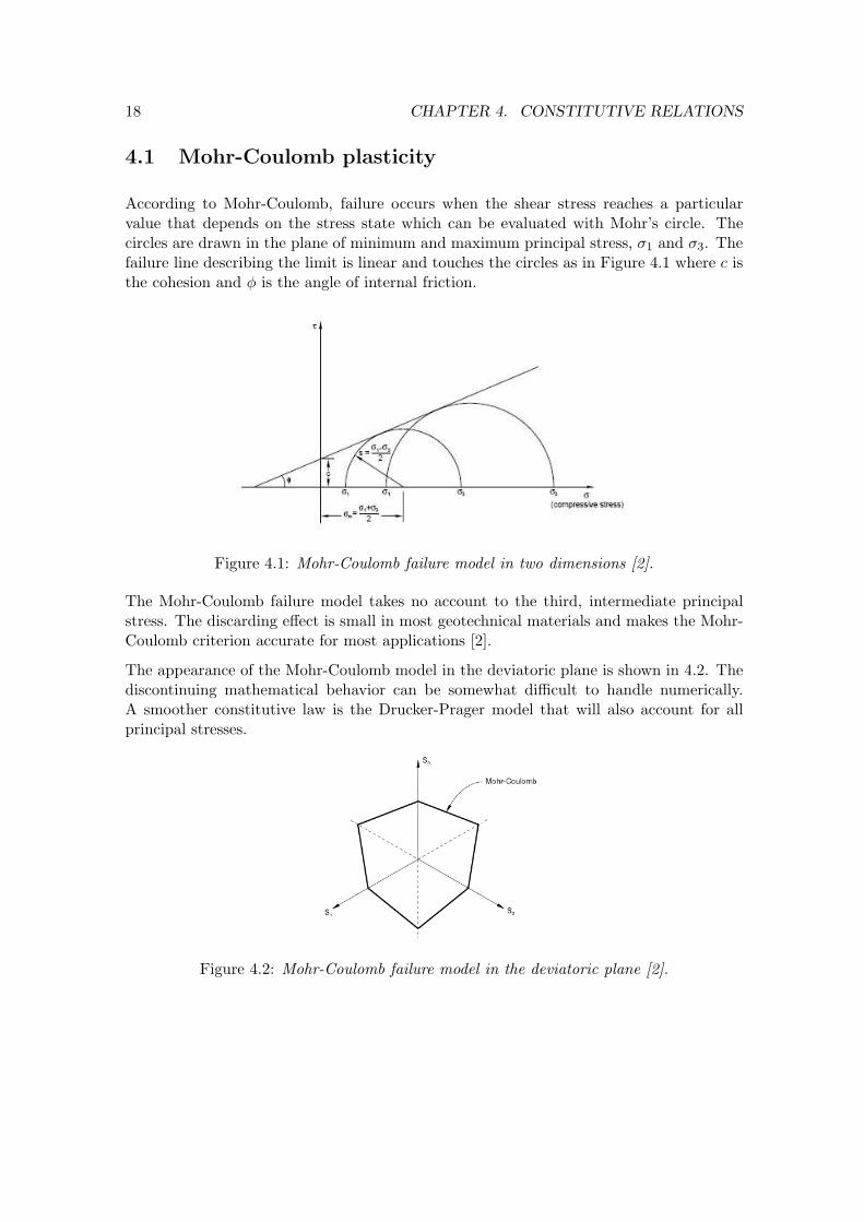
According to Mohr-Coulomb, failure occurs when the shear stress reaches a particularvalue that depends on the stress state which can be evaluated with Mohr’s circle. Thecircles are drawn in the plane of minimum and maximum principal stress, σ1 and σ3. Thefailure line describing the limit is linear and touches the circles as in Figure 4.1 where c isthe cohesion and φ is the angle of internal friction.

Figure 4.1: Mohr-Coulomb failure model in two dimensions [2].

The Mohr-Coulomb failure model takes no account to the third, intermediate principalstress. The discarding effect is small in most geotechnical materials and makes the Mohr-Coulomb criterion accurate for most applications [2].

The appearance of the Mohr-Coulomb model in the deviatoric plane is shown in 4.2. Thediscontinuing mathematical behavior can be somewhat difficult to handle numerically.A smoother constitutive law is the Drucker-Prager model that will also account for allprincipal stresses.

Figure 4.2: Mohr-Coulomb failure model in the deviatoric plane [2].

4.2. DRUCKER-PRAGER PLASTICITY 19

4.2 Drucker-Prager plasticity

The Drucker-Prager model takes account for all principal stresses. In its most genericform, the criterion is stated in terms of the first stress invariant I1 and the second stressdeviator invariant J2 as [7]

F (I1, J2) = 0 (4.1)

where

I1 = σii (4.2)

I2 =12σijσji (4.3)

J2 = I2 − 16I21 (4.4)

The explicit and linear form of (4.1) for a nondilatant material is a relation between I1

and√

J2 stated in

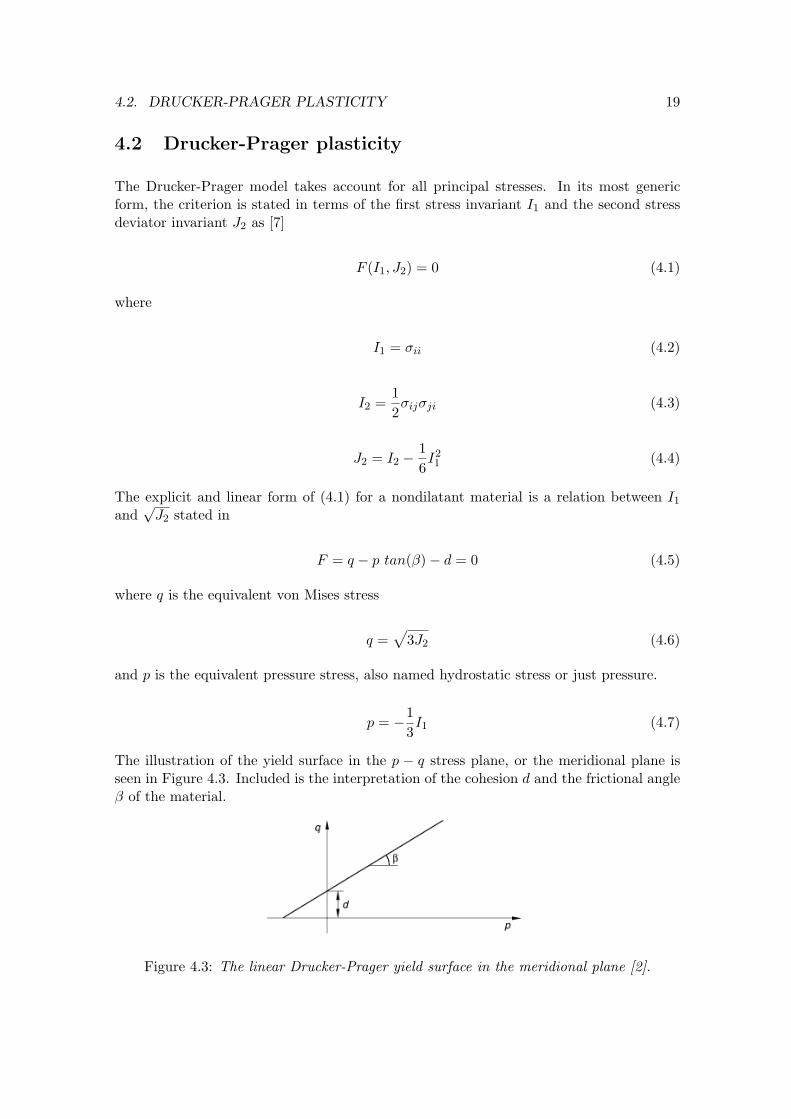
F = q − p tan(β)− d = 0 (4.5)

where q is the equivalent von Mises stress

q =√

3J2 (4.6)

and p is the equivalent pressure stress, also named hydrostatic stress or just pressure.

p = −13I1 (4.7)

The illustration of the yield surface in the p − q stress plane, or the meridional plane isseen in Figure 4.3. Included is the interpretation of the cohesion d and the frictional angleβ of the material.

Figure 4.3: The linear Drucker-Prager yield surface in the meridional plane [2].

20 CHAPTER 4. CONSTITUTIVE RELATIONS

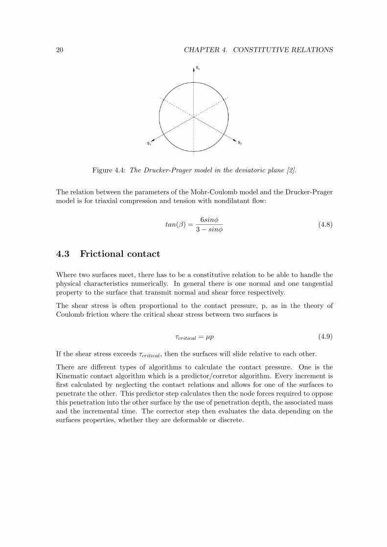
Figure 4.4: The Drucker-Prager model in the deviatoric plane [2].

The relation between the parameters of the Mohr-Coulomb model and the Drucker-Pragermodel is for triaxial compression and tension with nondilatant flow:

tan(β) =6sinφ

3− sinφ(4.8)

4.3 Frictional contact

Where two surfaces meet, there has to be a constitutive relation to be able to handle thephysical characteristics numerically. In general there is one normal and one tangentialproperty to the surface that transmit normal and shear force respectively.

The shear stress is often proportional to the contact pressure, p, as in the theory ofCoulomb friction where the critical shear stress between two surfaces is

τcritical = µp (4.9)

If the shear stress exceeds τcritical, then the surfaces will slide relative to each other.

There are different types of algorithms to calculate the contact pressure. One is theKinematic contact algorithm which is a predictor/corretor algorithm. Every increment isfirst calculated by neglecting the contact relations and allows for one of the surfaces topenetrate the other. This predictor step calculates then the node forces required to opposethis penetration into the other surface by the use of penetration depth, the associated massand the incremental time. The corrector step then evaluates the data depending on thesurfaces properties, whether they are deformable or discrete.

Chapter 5

Simulation conditions

As the simulation has to be performed with an Eulerian description, the time history dataof the discharge cannot be captured. Even if it were possible to simulate the upper surfacewith a Lagrangian description, the physical discharge time is as long as 13 hours and wouldbe impractical to calculate. Therefore the simulations have to be done at specific states.The states can be found by evaluating and discuss the result of the previous simulatedstates.

The forces acting on the pellets are gravitational and frictional forces. The gravitationalforce will cause a compaction of the pellets immediately when the simulation begins andwill disturb the location of the tracer particles with an unnatural movement. Thereforethe simulation needs a first step, where the compaction is simulated, and thereafter asecond step where the outlet will be opened. The first step also gives the static stresscondition. To avoid unwished transients the applying of the gravity force and the openingof the outlet should be simulated smoothly.

5.1 Density

The density of interest for modelling the pellets as a continuum is the bulk density whichis 2300 kg/m3.

5.2 Elasticity

The elasticity module and the lateral contraction ratio is ambiguous. In the work ofGustafsson [4] it is indicated that both the modulus of elasticity and the Poissont’s ratiodepend on the stress state, however the dependency is not fully investigated. The valuesare then set to consist of average values from the current work.

The simulations will have an elastic modulus of 2.4 MPa and a Poisson’s ratio of 0.4.

21

22 CHAPTER 5. SIMULATION CONDITIONS

5.3 Plasticity

The plasticity part in the constitutive relation is described by the Drucker-Prager failuremodel. The angle of internal friction is assumed equal to the angle of repose evaluated by[6]. The angle of repose is found to be about 26◦, which is also claimed in the EuropeanStandard [1]. The European Standard is also claiming that the angle of internal frictionis somewhat higher than the angle of repose, about 31◦.

If the angle of 26◦ is assumed to be the internal friction of the Mohr-Coulomb failuremodel, φ, it is needed to be recalculated to obtain the angle of internal friction of theDrucker-Prager failure model, β as

β = tan−1

(6sin26

3− sin26

)= 46 (5.1)

It is the same value as Gustafsson [4] found, and is therefore settled as the most interestingvalue. But it is still of interest to simulate how eventual fluctuations, in the angle of internalfriction, will influence on the stresses and the flow pattern in the silo.

5.4 Friction

The friction is a property with large impact on the result. The lower the friction is, thehigher the stresses will be in the pellets. More force will be received in the bottom ofthe silo where more horizontal surfaces exist. If the material fails along the walls, higherfriction coefficients will have no impact on the stresses.

The friction coefficients, between iron ore pellets and the walls, is found in the EuropeanStandard [1]. The values are formulated as an average value and a modification coefficientto give upper and lower characteristic values.

For a wall type D2, which is defined as steel finished concrete and carbon steel with lightsurface rust, the average value is µ = 0.54 with upper characteristic value of 0.6 and lowerof 0.48. For a wall type D3, which is defined as off-form concrete, the average value is 0.59with upper characteristic value of 0.66 and lower of 0.53.

The inner tube will be made of off-form concrete and the silo walls of blasted bedrock.The inner tube is of a wall type D3, however the walls of bedrock are harder to evaluate.As pellets in the outer part of the silo are expected to be in a static condition, the frictioncoefficient are not that important as inside the inner tube. In the hopper, located insidethe inner tube, the pellets will move and the friction coefficient is therefore important.The hopper can be covered by steel plates to give low friction coefficients and is in thatcase a wall of type D2. Otherwise the friction coefficient is assumed to be ”high”.

It is of interest to simulate how larger fluctuations of the friction coefficient will affect thestresses and the flow pattern.

5.5. BOUNDARIES 23

5.5 Boundaries

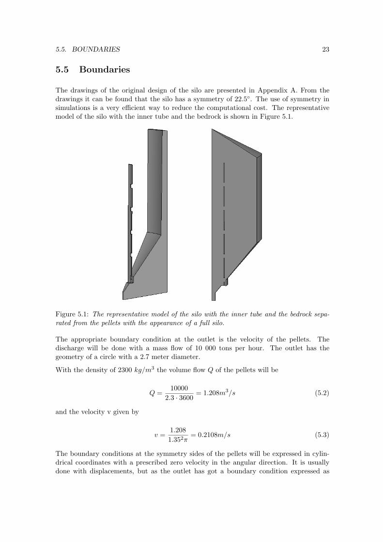
The drawings of the original design of the silo are presented in Appendix A. From thedrawings it can be found that the silo has a symmetry of 22.5◦. The use of symmetry insimulations is a very efficient way to reduce the computational cost. The representativemodel of the silo with the inner tube and the bedrock is shown in Figure 5.1.

Figure 5.1: The representative model of the silo with the inner tube and the bedrock sepa-rated from the pellets with the appearance of a full silo.

The appropriate boundary condition at the outlet is the velocity of the pellets. Thedischarge will be done with a mass flow of 10 000 tons per hour. The outlet has thegeometry of a circle with a 2.7 meter diameter.

With the density of 2300 kg/m3 the volume flow Q of the pellets will be

Q =10000

2.3 · 3600= 1.208m3/s (5.2)

and the velocity v given by

v =1.2081.352π

= 0.2108m/s (5.3)

The boundary conditions at the symmetry sides of the pellets will be expressed in cylin-drical coordinates with a prescribed zero velocity in the angular direction. It is usuallydone with displacements, but as the outlet has got a boundary condition expressed as

24 CHAPTER 5. SIMULATION CONDITIONS

prescribed velocity, it will cause difficulties at the edges that are separating two surfaceswith different types of boundary conditions.

The vertical line in the center of the model will have a prescribed velocity of zero in theradial direction in a cylindrical coordinate system. The reason to describe the conditionas prescribed velocity is the same as for the symmetry sides.

The inlet at the upper surface will have no boundary condition, more than the meshconstraint, that makes the mesh domain Eulerian. Material will be free to flow acrossthe surface and ”fill” the mesh as the silo discharges. During the first step, when thecompaction is simulated, it will be possible to see if the assumed surface in the currentstate is stable. If it is not, there will be a flow indication.

5.6 Stresses and strain

The limit of 250 kPa vertical stress is evaluated from tests made inside a rubber cylinderwith an axial load and a horizontal displacement between the upper and lower circularsurfaces. The vertical stress limit is taken from the axial load with a good margin. As theshear stress state in the cylinder is not known, it could be of interest to evaluate not onlythe vertical stresses but also the principal stress.

Equivalent plastic strain or PEEQ, is an interesting parameter that can show where thematerial has plastic strain. The plastic strain indicates yield surfaces that can be of interestin the analysis. It is defined by

PEEQ =∫ t

0ε̇pldt (5.4)

Where ε̇pl is the strain rate in uniaxial compression.

Part III

Result

25

Chapter 6

Original design

This chapter evaluates the silo in its original design, as it is established by LKAB incollaboration with specialists on the subject. Experimental scale tests on silos both withand without an inner tube are done as a part of the design process.

There are mainly two reasons of having an inner tube. At first it is thought that it reducesthe stresses in the pellets by reducing movement to inside the tube. The second reasonis that if the pellets are mostly discharging through the upper opening, while having auniform velocity inside the tube, then it is possible to have almost full control over thetraceability. This will produce an artificial pipe flow.

By first looking at the classical silo design, shown in Figure 2.3, with a friction coefficientof about 0.5, with the internal friction of the pellets set to 26◦ and with a slope in thehopper of 40◦, a funnel flow could be expected. This will ruin the traceability criterion ifthe bulk inside the tube is mixed.

The angle of the hopper will have to be as precipitous as 20◦ or the friction coefficienthas to be reduced to 0.2 to give a mass flow inside the inner tube. The diagram assumesa perfect silo. The original design also has a plateau at the transition between the innertube and the hopper. The plateau is for supporting scaffolding during construction.

In terms of stress, a high friction coefficient will give low stresses in the pellets but highforces on the structure. In terms of flow pattern, high friction coefficients will tend tomake the flow a funnel flow inside the inner tube and low friction coefficients will tend theflow to become a mass flow.

The characteristics of the influence from the friction coefficient is therefore complex.Higher as well as lower coefficients are of interest since low coefficients give high stresseswhile high coefficients give the presumed unwished funnel flow.

The upper bound of the friction coefficient is used to evaluate the flow profile since it ispreventing a mass flow. The lower bound is used to evaluate the stress condition. If thereis mass flow, at high friction coefficients, there will also be a mass flow at low frictioncoefficients.

27

28 CHAPTER 6. ORIGINAL DESIGN

6.1 Discharge state 1

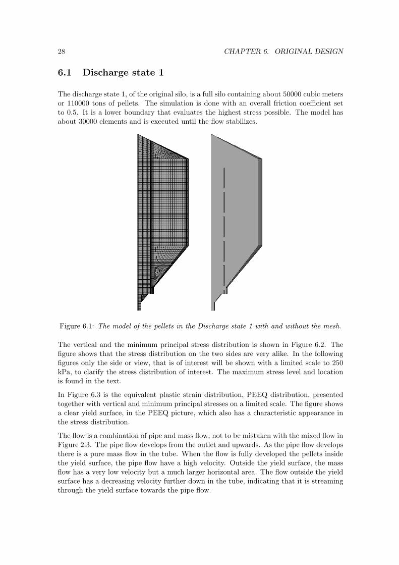
The discharge state 1, of the original silo, is a full silo containing about 50000 cubic metersor 110000 tons of pellets. The simulation is done with an overall friction coefficient setto 0.5. It is a lower boundary that evaluates the highest stress possible. The model hasabout 30000 elements and is executed until the flow stabilizes.

Figure 6.1: The model of the pellets in the Discharge state 1 with and without the mesh.

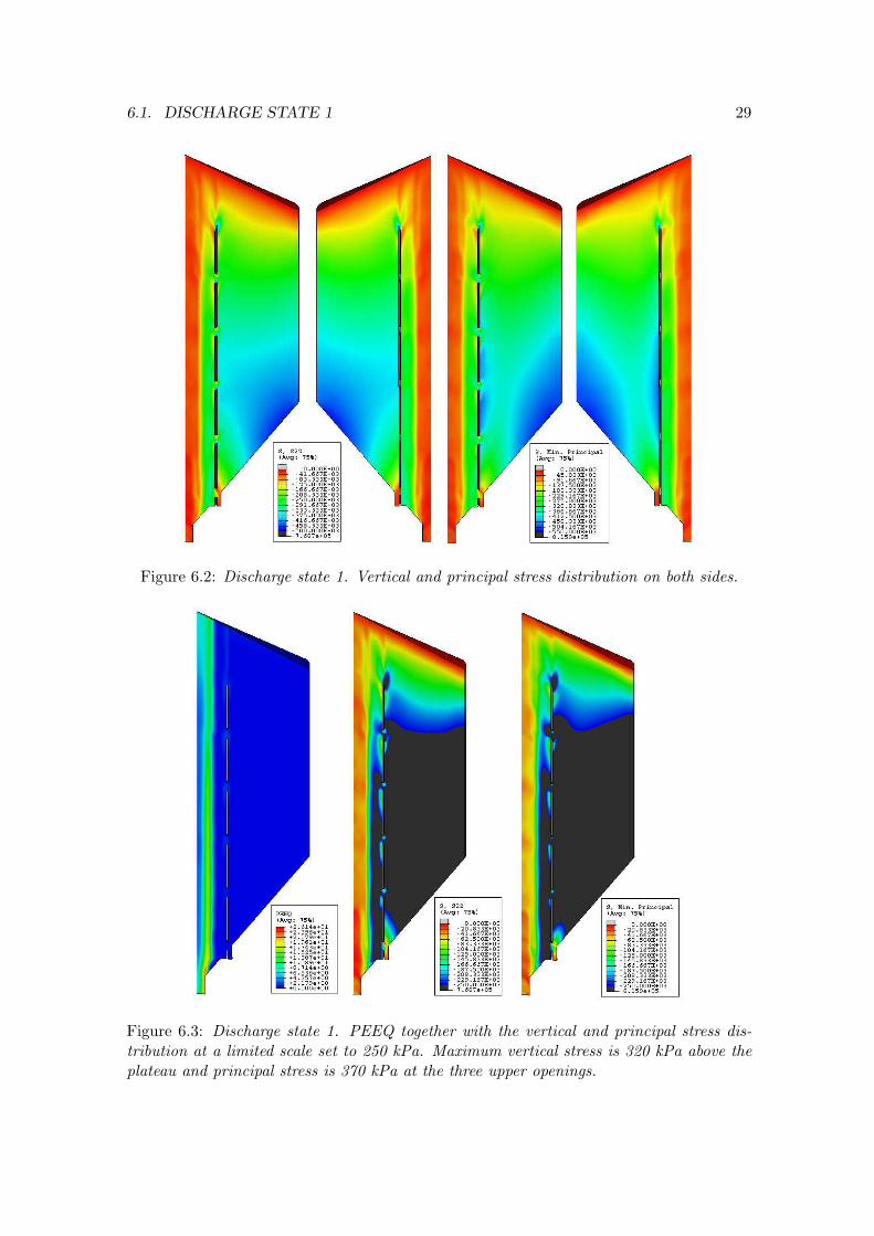
The vertical and the minimum principal stress distribution is shown in Figure 6.2. Thefigure shows that the stress distribution on the two sides are very alike. In the followingfigures only the side or view, that is of interest will be shown with a limited scale to 250kPa, to clarify the stress distribution of interest. The maximum stress level and locationis found in the text.

In Figure 6.3 is the equivalent plastic strain distribution, PEEQ distribution, presentedtogether with vertical and minimum principal stresses on a limited scale. The figure showsa clear yield surface, in the PEEQ picture, which also has a characteristic appearance inthe stress distribution.

The flow is a combination of pipe and mass flow, not to be mistaken with the mixed flow inFigure 2.3. The pipe flow develops from the outlet and upwards. As the pipe flow developsthere is a pure mass flow in the tube. When the flow is fully developed the pellets insidethe yield surface, the pipe flow have a high velocity. Outside the yield surface, the massflow has a very low velocity but a much larger horizontal area. The flow outside the yieldsurface has a decreasing velocity further down in the tube, indicating that it is streamingthrough the yield surface towards the pipe flow.

6.1. DISCHARGE STATE 1 29

Figure 6.2: Discharge state 1. Vertical and principal stress distribution on both sides.

Figure 6.3: Discharge state 1. PEEQ together with the vertical and principal stress dis-tribution at a limited scale set to 250 kPa. Maximum vertical stress is 320 kPa above theplateau and principal stress is 370 kPa at the three upper openings.


A calculation at the top of the inner tube shows that the pipe flow is around 1.1 m3/s andthe mass flow 0.1 m3/s. A light yield surface can be seen above the top of the inner tubethat is separating the mass flow from the surrounding pellets. Then the outflow consistsup to 10% of pellets that have an uncertain origin. It is possible that they have had theirway through with high stress areas.

The maximum vertical stress is 320 kPa and the maximum principal stress is as most 370kPa, both located outside the yield surface in the mass flow. The highest vertical stress islocated above the plateau, in the bottom of the inner tube and the highest principal stressis found at the openings. The vertical stress is influenced by the horizontal surface andthe principal stress by shear stress from the opening’s horizontal surface. The principalstress is highest at the three openings at the top where the velocity is higher than furtherdown. There is no flow through the openings.

6.1.1 Impact of the friction coefficient µ

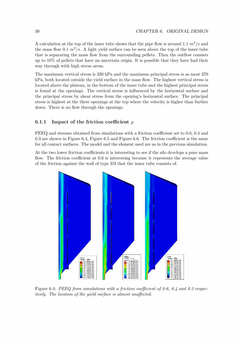
PEEQ and stresses obtained from simulations with a friction coefficient set to 0.6, 0.4 and0.3 are shown in Figure 6.4, Figure 6.5 and Figure 6.6. The friction coefficient is the samefor all contact surfaces. The model and the element used are as in the previous simulation.

At the two lower friction coefficients it is interesting to see if the silo develops a pure massflow. The friction coefficient at 0.6 is interesting because it represents the average valueof the friction against the wall of type D3 that the inner tube consists of.

Figure 6.4: PEEQ from simulations with a friction coefficient of 0.6, 0.4 and 0.3 respec-tively. The location of the yield surface is almost unaffected.


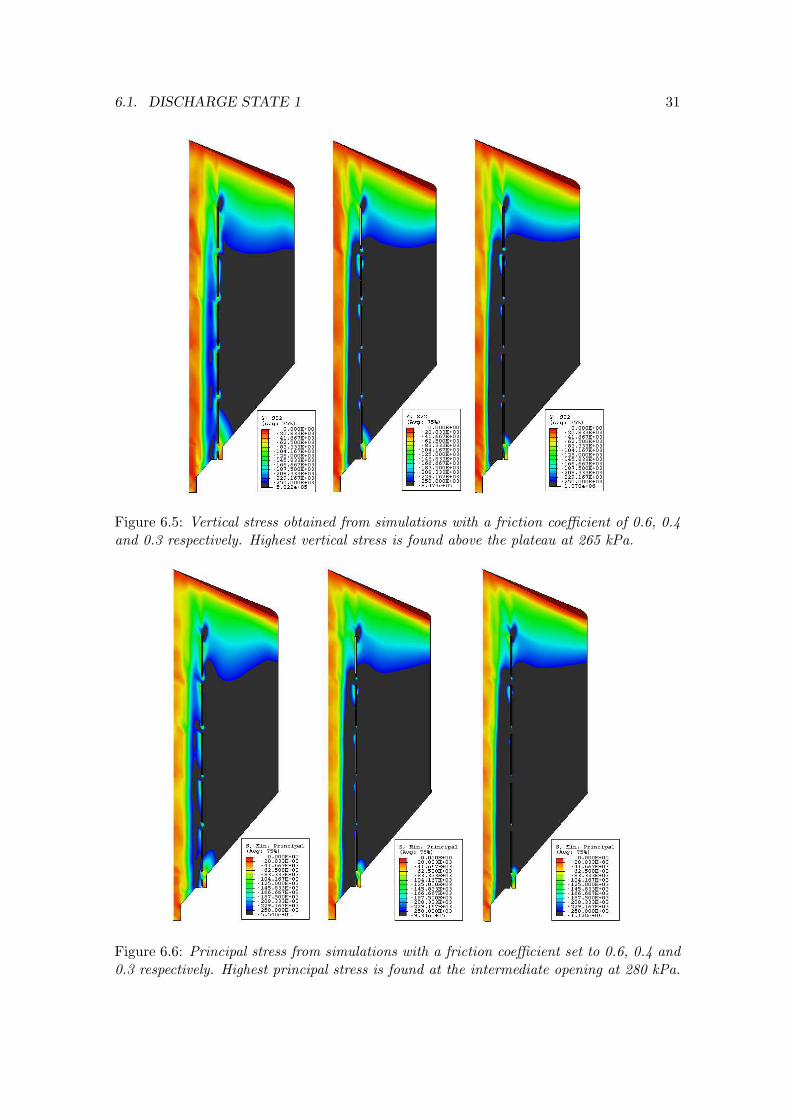
Figure 6.5: Vertical stress obtained from simulations with a friction coefficient of 0.6, 0.4and 0.3 respectively. Highest vertical stress is found above the plateau at 265 kPa.

Figure 6.6: Principal stress from simulations with a friction coefficient set to 0.6, 0.4 and0.3 respectively. Highest principal stress is found at the intermediate opening at 280 kPa.


The location of the yield surface and the flow pattern is almost unaffected by the changes.The silo has no tendency to develop a mass flow at these friction coefficients. The stressesare decreased when the friction is higher and are increased when the friction is lowered asit was assumed. At the friction coefficient 0.6 the maximum vertical stress is reduced to265 kPa and the maximum principal stress to 280 kPa.

6.1.2 Impact of the material parameter β

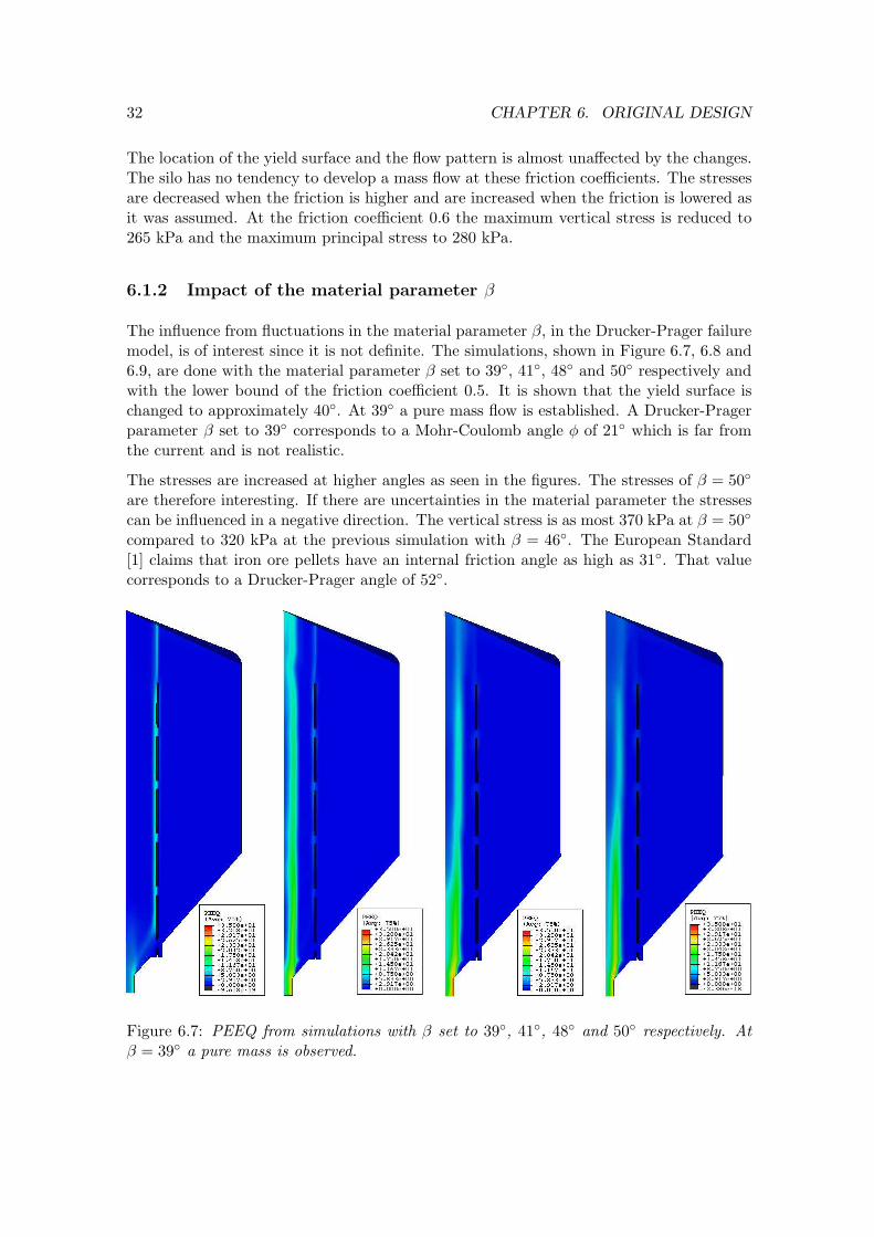
The influence from fluctuations in the material parameter β, in the Drucker-Prager failuremodel, is of interest since it is not definite. The simulations, shown in Figure 6.7, 6.8 and6.9, are done with the material parameter β set to 39◦, 41◦, 48◦ and 50◦ respectively andwith the lower bound of the friction coefficient 0.5. It is shown that the yield surface ischanged to approximately 40◦. At 39◦ a pure mass flow is established. A Drucker-Pragerparameter β set to 39◦ corresponds to a Mohr-Coulomb angle φ of 21◦ which is far fromthe current and is not realistic.

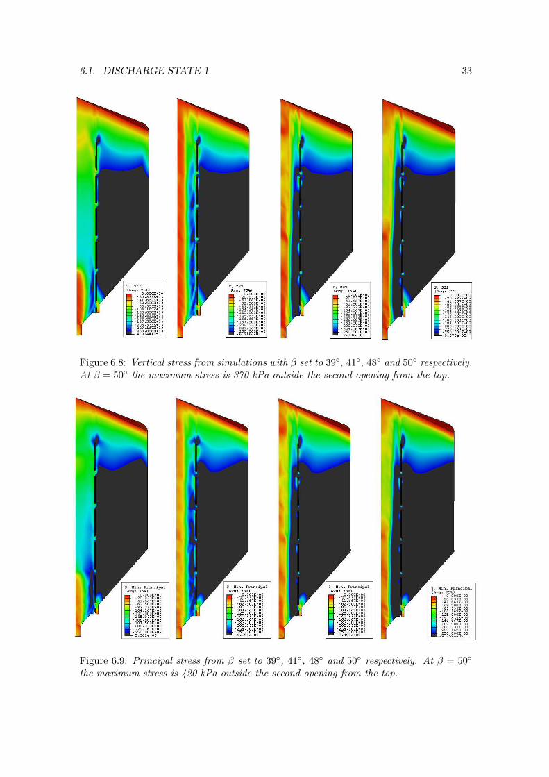
The stresses are increased at higher angles as seen in the figures. The stresses of β = 50◦

are therefore interesting. If there are uncertainties in the material parameter the stressescan be influenced in a negative direction. The vertical stress is as most 370 kPa at β = 50◦

compared to 320 kPa at the previous simulation with β = 46◦. The European Standard[1] claims that iron ore pellets have an internal friction angle as high as 31◦. That valuecorresponds to a Drucker-Prager angle of 52◦.

Figure 6.7: PEEQ from simulations with β set to 39◦, 41◦, 48◦ and 50◦ respectively. Atβ = 39◦ a pure mass is observed.


Figure 6.8: Vertical stress from simulations with β set to 39◦, 41◦, 48◦ and 50◦ respectively.At β = 50◦ the maximum stress is 370 kPa outside the second opening from the top.

Figure 6.9: Principal stress from β set to 39◦, 41◦, 48◦ and 50◦ respectively. At β = 50◦

the maximum stress is 420 kPa outside the second opening from the top.



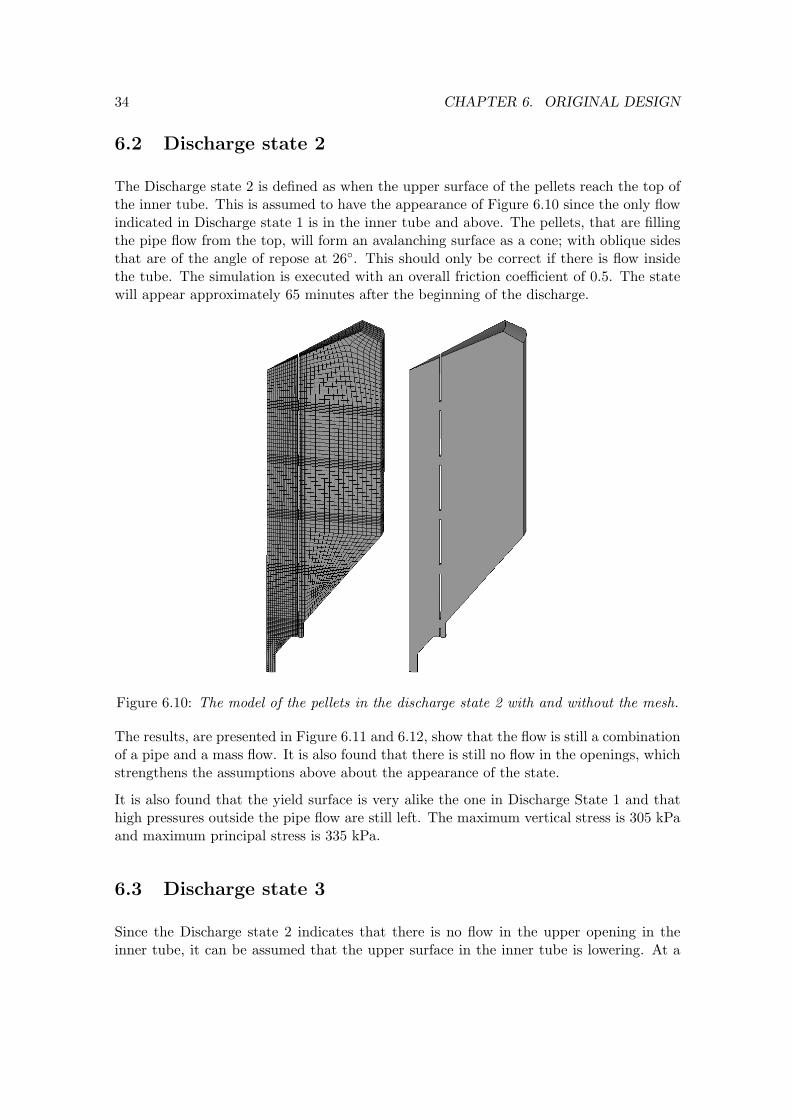
The Discharge state 2 is defined as when the upper surface of the pellets reach the top ofthe inner tube. This is assumed to have the appearance of Figure 6.10 since the only flowindicated in Discharge state 1 is in the inner tube and above. The pellets, that are fillingthe pipe flow from the top, will form an avalanching surface as a cone; with oblique sidesthat are of the angle of repose at 26◦. This should only be correct if there is flow insidethe tube. The simulation is executed with an overall friction coefficient of 0.5. The statewill appear approximately 65 minutes after the beginning of the discharge.

Figure 6.10: The model of the pellets in the discharge state 2 with and without the mesh.

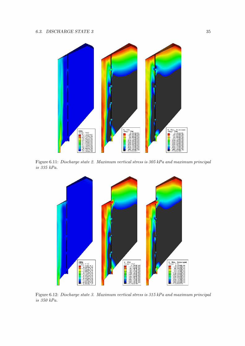
The results, are presented in Figure 6.11 and 6.12, show that the flow is still a combinationof a pipe and a mass flow. It is also found that there is still no flow in the openings, whichstrengthens the assumptions above about the appearance of the state.

It is also found that the yield surface is very alike the one in Discharge State 1 and thathigh pressures outside the pipe flow are still left. The maximum vertical stress is 305 kPaand maximum principal stress is 335 kPa.


Since the Discharge state 2 indicates that there is no flow in the upper opening in theinner tube, it can be assumed that the upper surface in the inner tube is lowering. At a


Figure 6.11: Discharge state 2. Maximum vertical stress is 305 kPa and maximum principalis 335 kPa.

Figure 6.12: Discharge state 3. Maximum vertical stress is 315 kPa and maximum principalis 350 kPa.


certain level the pressure difference, at the opening, will be high enough to cause a flowthrough it.

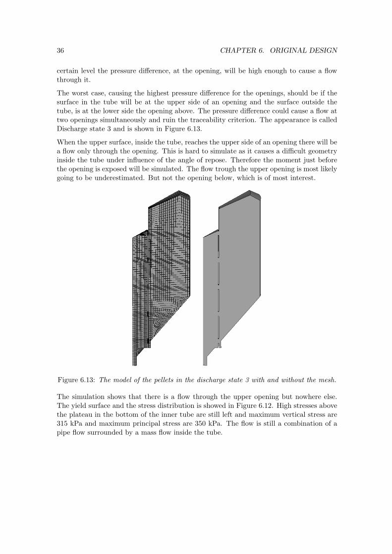
The worst case, causing the highest pressure difference for the openings, should be if thesurface in the tube will be at the upper side of an opening and the surface outside thetube, is at the lower side the opening above. The pressure difference could cause a flow attwo openings simultaneously and ruin the traceability criterion. The appearance is calledDischarge state 3 and is shown in Figure 6.13.

When the upper surface, inside the tube, reaches the upper side of an opening there will bea flow only through the opening. This is hard to simulate as it causes a difficult geometryinside the tube under influence of the angle of repose. Therefore the moment just beforethe opening is exposed will be simulated. The flow trough the upper opening is most likelygoing to be underestimated. But not the opening below, which is of most interest.

Figure 6.13: The model of the pellets in the discharge state 3 with and without the mesh.

The simulation shows that there is a flow through the upper opening but nowhere else.The yield surface and the stress distribution is showed in Figure 6.12. High stresses abovethe plateau in the bottom of the inner tube are still left and maximum vertical stress are315 kPa and maximum principal stress are 350 kPa. The flow is still a combination of apipe flow surrounded by a mass flow inside the tube.

Chapter 7

Modified design

With knowledge of the conditions in the original design of the silo it is of interest toinvestigate the effects of modified designs.

37

38 CHAPTER 7. MODIFIED DESIGN

7.1 No inner tube

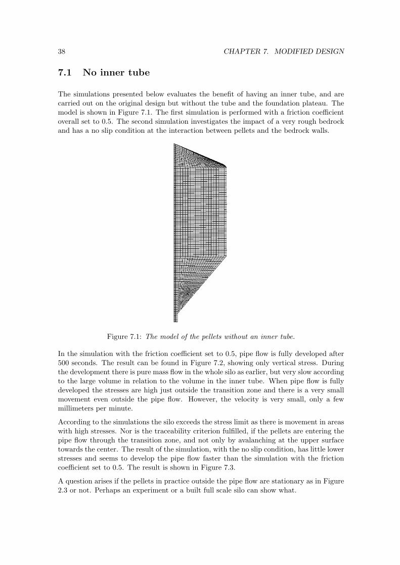
The simulations presented below evaluates the benefit of having an inner tube, and arecarried out on the original design but without the tube and the foundation plateau. Themodel is shown in Figure 7.1. The first simulation is performed with a friction coefficientoverall set to 0.5. The second simulation investigates the impact of a very rough bedrockand has a no slip condition at the interaction between pellets and the bedrock walls.

Figure 7.1: The model of the pellets without an inner tube.

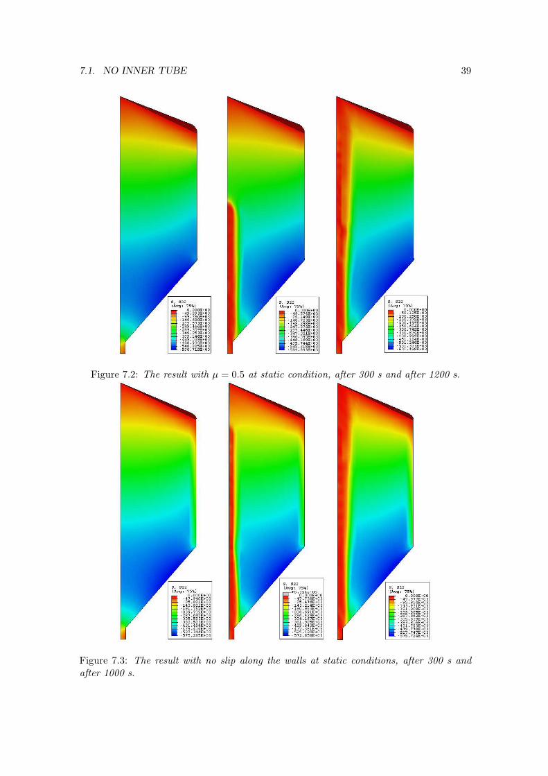
In the simulation with the friction coefficient set to 0.5, pipe flow is fully developed after500 seconds. The result can be found in Figure 7.2, showing only vertical stress. Duringthe development there is pure mass flow in the whole silo as earlier, but very slow accordingto the large volume in relation to the volume in the inner tube. When pipe flow is fullydeveloped the stresses are high just outside the transition zone and there is a very smallmovement even outside the pipe flow. However, the velocity is very small, only a fewmillimeters per minute.

According to the simulations the silo exceeds the stress limit as there is movement in areaswith high stresses. Nor is the traceability criterion fulfilled, if the pellets are entering thepipe flow through the transition zone, and not only by avalanching at the upper surfacetowards the center. The result of the simulation, with the no slip condition, has little lowerstresses and seems to develop the pipe flow faster than the simulation with the frictioncoefficient set to 0.5. The result is shown in Figure 7.3.

A question arises if the pellets in practice outside the pipe flow are stationary as in Figure2.3 or not. Perhaps an experiment or a built full scale silo can show what.

7.1. NO INNER TUBE 39

Figure 7.2: The result with µ = 0.5 at static condition, after 300 s and after 1200 s.

Figure 7.3: The result with no slip along the walls at static conditions, after 300 s andafter 1000 s.


7.2 Design modification 1 - Oblique plateau

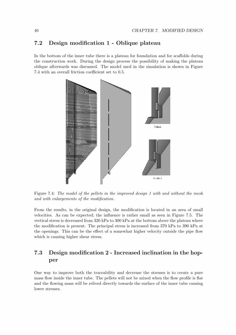
In the bottom of the inner tube there is a plateau for foundation and for scaffolds duringthe construction work. During the design process the possibility of making the plateauoblique afterwards was discussed. The model used in the simulation is shown in Figure7.4 with an overall friction coefficient set to 0.5.

Figure 7.4: The model of the pellets in the improved design 1 with and without the meshand with enlargements of the modification.

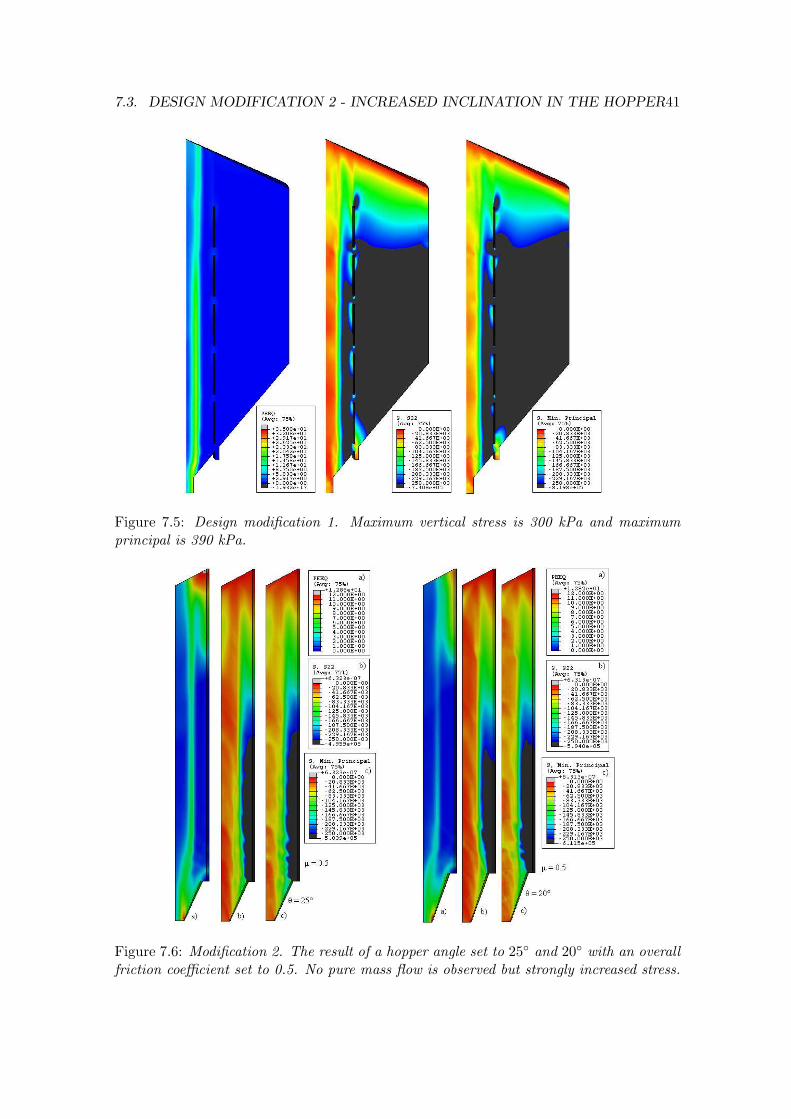
From the results, in the original design, the modification is located in an area of smallvelocities. As can be expected; the influence is rather small as seen in Figure 7.5. Thevertical stress is decreased from 320 kPa to 300 kPa at the bottom above the plateau wherethe modification is present. The principal stress is increased from 370 kPa to 390 kPa atthe openings. This can be the effect of a somewhat higher velocity outside the pipe flowwhich is causing higher shear stress.

7.3 Design modification 2 - Increased inclination in the hop-per

One way to improve both the traceability and decrease the stresses is to create a puremass flow inside the inner tube. The pellets will not be mixed when the flow profile is flatand the flowing mass will be relived directly towards the surface of the inner tube causinglower stresses.

7.3. DESIGN MODIFICATION 2 - INCREASED INCLINATION IN THE HOPPER41

Figure 7.5: Design modification 1. Maximum vertical stress is 300 kPa and maximumprincipal is 390 kPa.

Figure 7.6: Modification 2. The result of a hopper angle set to 25◦ and 20◦ with an overallfriction coefficient set to 0.5. No pure mass flow is observed but strongly increased stress.


To make the simulations more rational simply pellets inside the inner tube are evaluated.The simulations are performed simply to determine where it is possible to find a massflow. The stresses are showed in the results, but are not final because the openings arenot present.

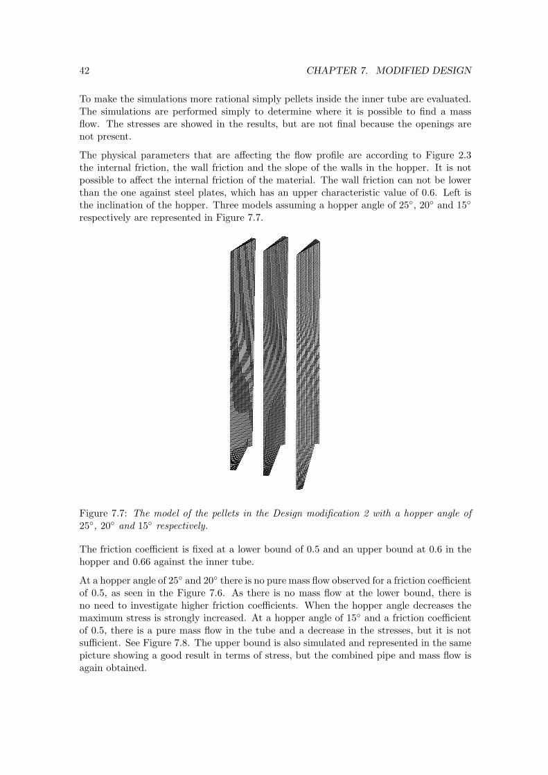
The physical parameters that are affecting the flow profile are according to Figure 2.3the internal friction, the wall friction and the slope of the walls in the hopper. It is notpossible to affect the internal friction of the material. The wall friction can not be lowerthan the one against steel plates, which has an upper characteristic value of 0.6. Left isthe inclination of the hopper. Three models assuming a hopper angle of 25◦, 20◦ and 15◦

respectively are represented in Figure 7.7.

Figure 7.7: The model of the pellets in the Design modification 2 with a hopper angle of25◦, 20◦ and 15◦ respectively.

The friction coefficient is fixed at a lower bound of 0.5 and an upper bound at 0.6 in thehopper and 0.66 against the inner tube.

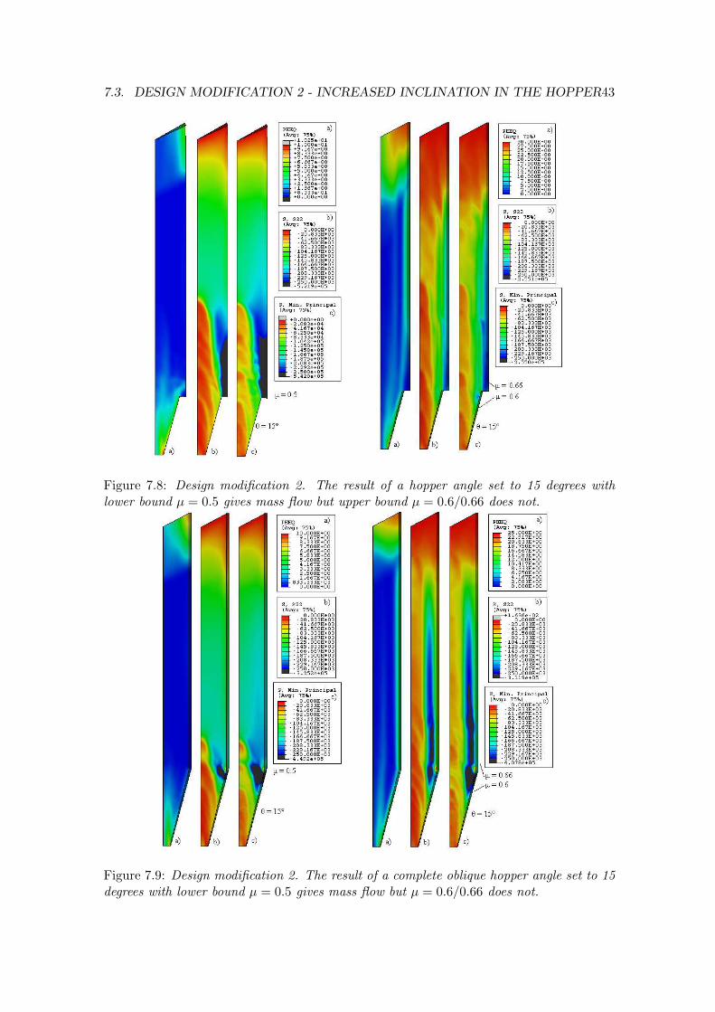
At a hopper angle of 25◦ and 20◦ there is no pure mass flow observed for a friction coefficientof 0.5, as seen in the Figure 7.6. As there is no mass flow at the lower bound, there isno need to investigate higher friction coefficients. When the hopper angle decreases themaximum stress is strongly increased. At a hopper angle of 15◦ and a friction coefficientof 0.5, there is a pure mass flow in the tube and a decrease in the stresses, but it is notsufficient. See Figure 7.8. The upper bound is also simulated and represented in the samepicture showing a good result in terms of stress, but the combined pipe and mass flow isagain obtained.

7.3. DESIGN MODIFICATION 2 - INCREASED INCLINATION IN THE HOPPER43

Figure 7.8: Design modification 2. The result of a hopper angle set to 15 degrees withlower bound µ = 0.5 gives mass flow but upper bound µ = 0.6/0.66 does not.

Figure 7.9: Design modification 2. The result of a complete oblique hopper angle set to 15degrees with lower bound µ = 0.5 gives mass flow but µ = 0.6/0.66 does not.


In Figure 7.9 the pellets inside the inner tube are simulated without the presence of theplateau and at a hopper angle of 15◦, both at the lower and upper bound of the frictioncoefficient. The figure shows that both higher stresses and the combined funnel and massflow is obtained without the influence of the plateau at this hopper angle.

By the original drawings in appendix A it can be noticed that the smallest angle possibleis 25◦. If lower angles are needed the underlaying tunnel has to be lowered or the diameterof the inner tube has to be smaller.

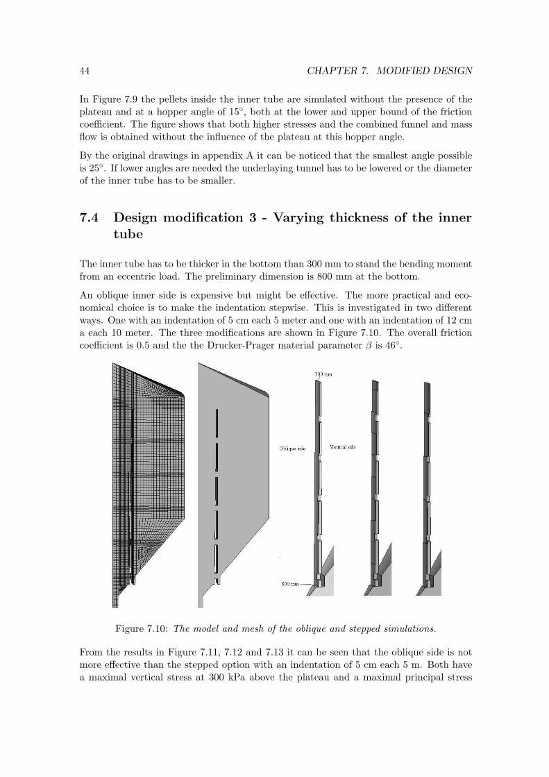
7.4 Design modification 3 - Varying thickness of the innertube

The inner tube has to be thicker in the bottom than 300 mm to stand the bending momentfrom an eccentric load. The preliminary dimension is 800 mm at the bottom.

An oblique inner side is expensive but might be effective. The more practical and eco-nomical choice is to make the indentation stepwise. This is investigated in two differentways. One with an indentation of 5 cm each 5 meter and one with an indentation of 12 cma each 10 meter. The three modifications are shown in Figure 7.10. The overall frictioncoefficient is 0.5 and the the Drucker-Prager material parameter β is 46◦.

Figure 7.10: The model and mesh of the oblique and stepped simulations.

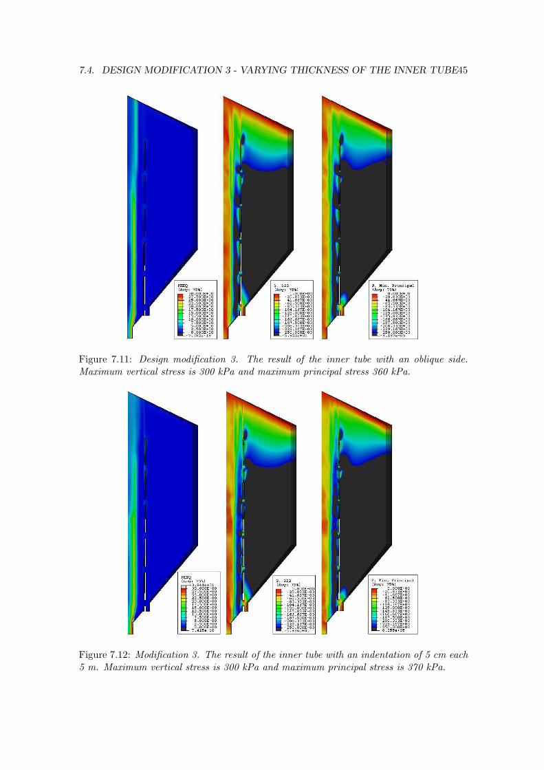
From the results in Figure 7.11, 7.12 and 7.13 it can be seen that the oblique side is notmore effective than the stepped option with an indentation of 5 cm each 5 m. Both havea maximal vertical stress at 300 kPa above the plateau and a maximal principal stress

7.4. DESIGN MODIFICATION 3 - VARYING THICKNESS OF THE INNER TUBE45

Figure 7.11: Design modification 3. The result of the inner tube with an oblique side.Maximum vertical stress is 300 kPa and maximum principal stress 360 kPa.

Figure 7.12: Modification 3. The result of the inner tube with an indentation of 5 cm each5 m. Maximum vertical stress is 300 kPa and maximum principal stress is 370 kPa.


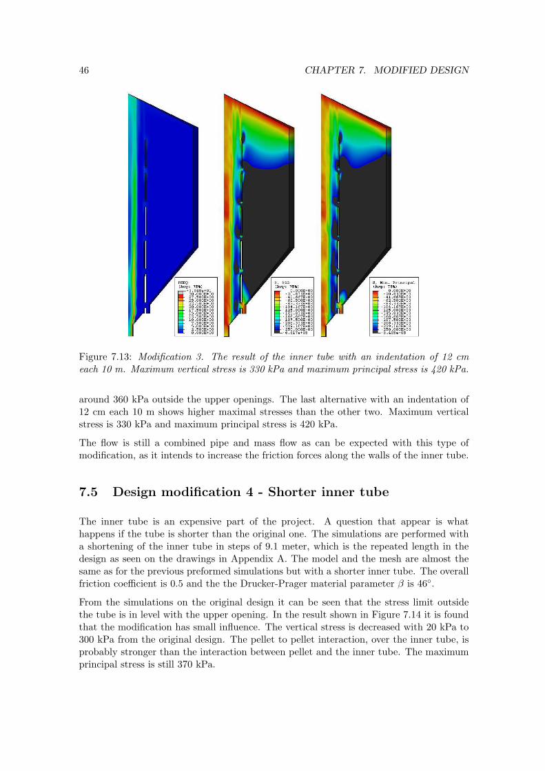
Figure 7.13: Modification 3. The result of the inner tube with an indentation of 12 cmeach 10 m. Maximum vertical stress is 330 kPa and maximum principal stress is 420 kPa.

around 360 kPa outside the upper openings. The last alternative with an indentation of12 cm each 10 m shows higher maximal stresses than the other two. Maximum verticalstress is 330 kPa and maximum principal stress is 420 kPa.

The flow is still a combined pipe and mass flow as can be expected with this type ofmodification, as it intends to increase the friction forces along the walls of the inner tube.

7.5 Design modification 4 - Shorter inner tube

The inner tube is an expensive part of the project. A question that appear is whathappens if the tube is shorter than the original one. The simulations are performed witha shortening of the inner tube in steps of 9.1 meter, which is the repeated length in thedesign as seen on the drawings in Appendix A. The model and the mesh are almost thesame as for the previous preformed simulations but with a shorter inner tube. The overallfriction coefficient is 0.5 and the the Drucker-Prager material parameter β is 46◦.

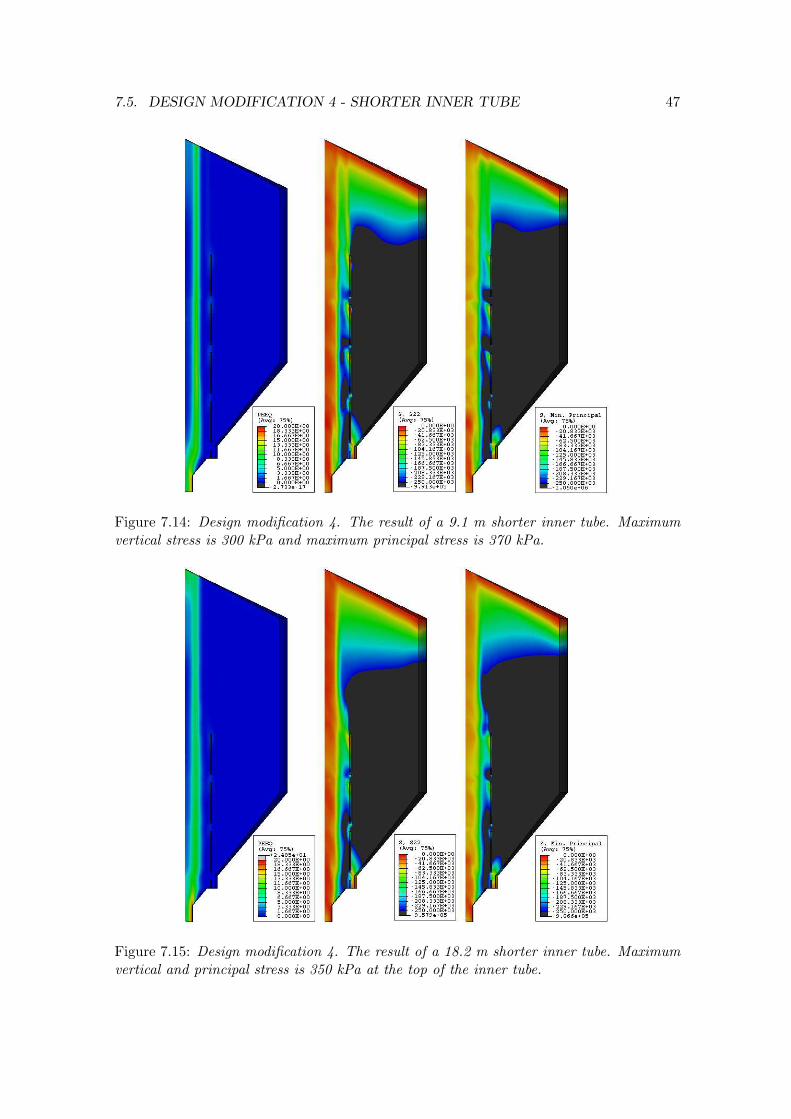
From the simulations on the original design it can be seen that the stress limit outsidethe tube is in level with the upper opening. In the result shown in Figure 7.14 it is foundthat the modification has small influence. The vertical stress is decreased with 20 kPa to300 kPa from the original design. The pellet to pellet interaction, over the inner tube, isprobably stronger than the interaction between pellet and the inner tube. The maximumprincipal stress is still 370 kPa.

7.5. DESIGN MODIFICATION 4 - SHORTER INNER TUBE 47

Figure 7.14: Design modification 4. The result of a 9.1 m shorter inner tube. Maximumvertical stress is 300 kPa and maximum principal stress is 370 kPa.

Figure 7.15: Design modification 4. The result of a 18.2 m shorter inner tube. Maximumvertical and principal stress is 350 kPa at the top of the inner tube.


When shorting the tube, by 18.2 m, the principal stress downwards the tube is also loweredwith 50 kPa to 320 kPa. But now there is an area at the top of the silo which has maximumvertical and principal stress at 350 kPa.

7.6 Design modification 5 - Decreased radius of the innertube

As seen from Design modification 2 with increased inclination in the hopper an inclinationlower than 15◦ is needed to obtain mass flow for the upper bound of the friction coefficient.The lower bound would on the other hand give very high stresses.

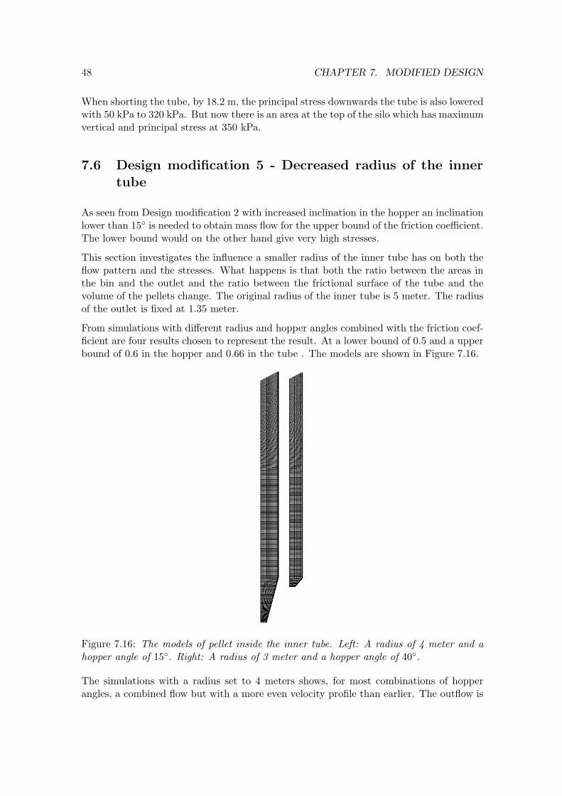
This section investigates the influence a smaller radius of the inner tube has on both theflow pattern and the stresses. What happens is that both the ratio between the areas inthe bin and the outlet and the ratio between the frictional surface of the tube and thevolume of the pellets change. The original radius of the inner tube is 5 meter. The radiusof the outlet is fixed at 1.35 meter.

From simulations with different radius and hopper angles combined with the friction coef-ficient are four results chosen to represent the result. At a lower bound of 0.5 and a upperbound of 0.6 in the hopper and 0.66 in the tube . The models are shown in Figure 7.16.

Figure 7.16: The models of pellet inside the inner tube. Left: A radius of 4 meter and ahopper angle of 15◦. Right: A radius of 3 meter and a hopper angle of 40◦.

The simulations with a radius set to 4 meters shows, for most combinations of hopperangles, a combined flow but with a more even velocity profile than earlier. The outflow is

7.6. DESIGN MODIFICATION 5 - DECREASED RADIUS OF THE INNER TUBE49

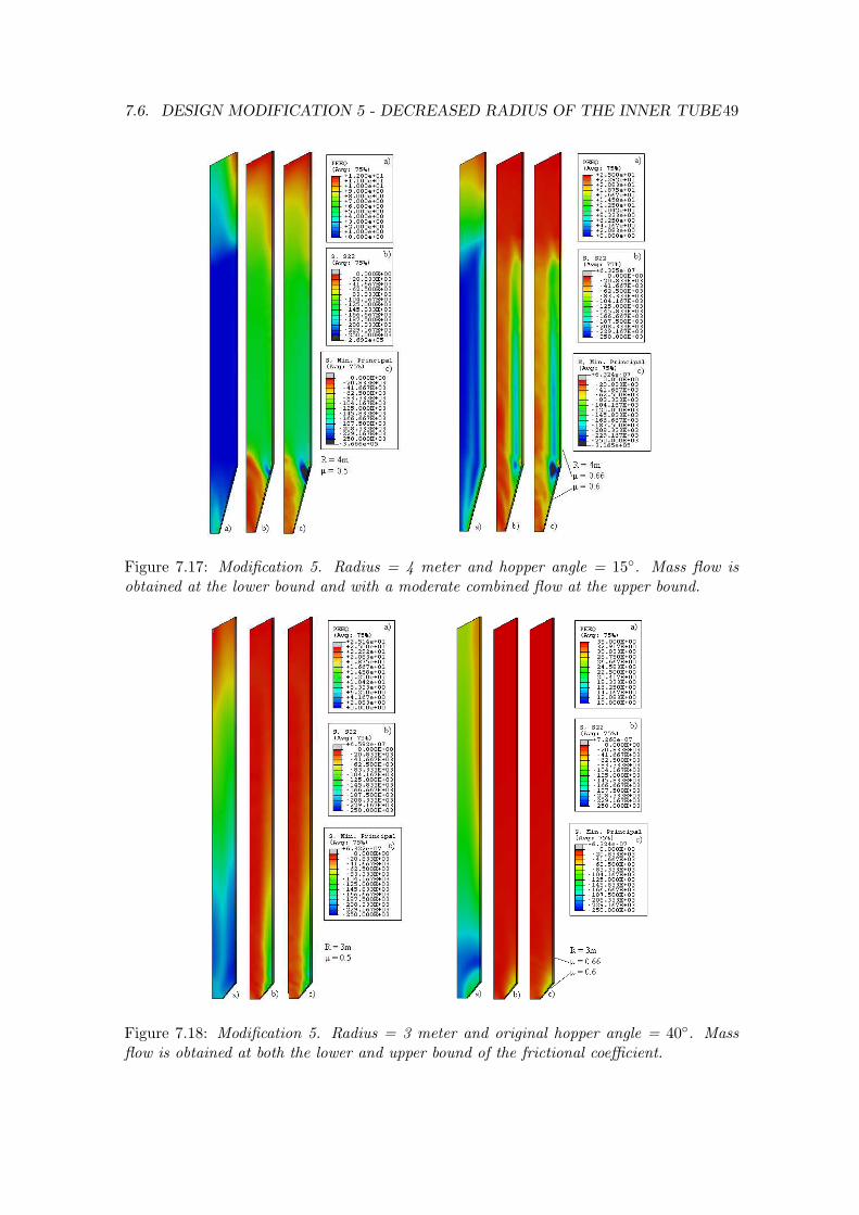
Figure 7.17: Modification 5. Radius = 4 meter and hopper angle = 15◦. Mass flow isobtained at the lower bound and with a moderate combined flow at the upper bound.

Figure 7.18: Modification 5. Radius = 3 meter and original hopper angle = 40◦. Massflow is obtained at both the lower and upper bound of the frictional coefficient.


still mixed with about 10% pellets but as the velocities are more equal improves this thetraceability. Only at a hopper angle of 15◦ is a pure mass flow is obtained for the lowerbound, at the upper bound is there a moderate combined flow. The simulations with aradius set to 4 meters and a hopper angle of 15◦ is presented in Figure 7.17.

The stresses are at a hopper angle of 40◦ about 360 kPa in both directions and at a hopperangle of 25◦ as high as 400 kPa vertical and 450 kPa in principal direction.

In Figure 7.18 the result is shown from a simulation with an inner radius of 3 meter and ahopper angle of 40◦ which is the original angle. For this radius mass flow is obtained, evenmoderate at the upper bound of the frictional coefficient. According to the simulationwith the lower bound maximum vertical stress is 205 kPa and the maximum principalstress is 215 kPa. At the upper bound of the frictional coefficient both the maximmumvertical and maximum principal stress is as low as about 85 kPa.

The ratio between the radius in the bin and at the outlet has, according to these simula-tions, influence on the flow pattern.

Part IV

Summary

51

Chapter 8

Summary

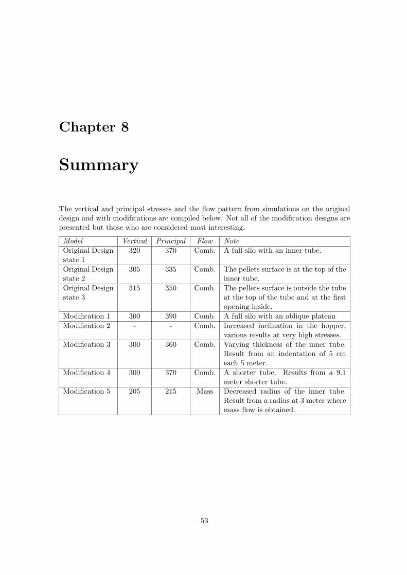
The vertical and principal stresses and the flow pattern from simulations on the originaldesign and with modifications are compiled below. Not all of the modification designs arepresented but those who are considered most interesting.

Model Vertical Principal Flow NoteOriginal Designstate 1

320 370 Comb. A full silo with an inner tube.

Original Designstate 2

305 335 Comb. The pellets surface is at the top of theinner tube.

Original Designstate 3

315 350 Comb. The pellets surface is outside the tubeat the top of the tube and at the firstopening inside.

Modification 1 300 390 Comb. A full silo with an oblique plateauModification 2 - - Comb. Increased inclination in the hopper,

various results at very high stresses.Modification 3 300 360 Comb. Varying thickness of the inner tube.

Result from an indentation of 5 cmeach 5 meter.

Modification 4 300 370 Comb. A shorter tube. Results from a 9.1meter shorter tube.

Modification 5 205 215 Mass Decreased radius of the inner tube.Result from a radius at 3 meter wheremass flow is obtained.

53

54 CHAPTER 8. SUMMARY

8.1 Conclusions

The original design has a combined pipe and mass flow inside the inner tube but nomovements in pellets outside the tube. The pellets in the outlet are mixed with about10% pellets with uncertain origin. The stresses are higher than the limit at 250 kPa in bothvertical and principal direction. The conditions are almost the same for all three simulatedstates making it an issue during a noticeable time. None of the smaller modifications onthe original design shows any big improvement but are of interest as basics for decisions.

The only modification that shows improvement is the one with an inner tube with a smallerradius than the original 5 meter. At a radius of 3 meters, mass flow is obtained even forthe original hopper angle at 40◦ together with low stresses.

The wall friction coefficient and the angle of internal friction in the pellets have influenceon the result. Higher friction coefficients give lower stress but counteract mass flow. Lowfriction coefficients tend to give mass flow but with high stresses. The internal frictionangle in the pellets, influence in such a way that it gives mass flow at low values and higherstress at higher values.

8.2 Discussion

The silo with the original design will probably have no problem with the stress levels as thethreshold is chosen with good margin, but from an economical point of view this margin isof interest. With a more detailed knowledge about the causes of the quality decreasing inthe pellets during mechanical influence, maybe a more custom made design is possible ora design that can have an increased focus on the pellets’ quality. Better knowledge in theeffects of stress influence on iron ore pellets will lead to a better economical use. Thereis a possibility that this knowledge will have large benefits as it is the most uncertainparameter in the simulations.

The parameters in the simulations that affect the result on a specific geometric designare the wall frictional coefficient and the internal friction angle. The more exact theparameters are known, the more accurate the simulations will be. In this thesis they havebeen executed with friction coefficients from the European standard and not from specifictests.

The most attractive design of the tube identified from the simulations is the one witha smaller radius than the original. The smaller radius gives mass flow for high frictioncoefficients and lower stresses. A smaller radius, however, gives the tube a decreasedmoment of inertia and will therefore probably meet engineering problems.

A lower tube is shown possible and should decrease the bending moment in the tube whichis a cantilever beam. To avoid problems caused by decreased moment of inertia, the tubecan be supported by beams or stays made of wires in the top. At the bottom it can besupported with plates from the bedrock. With a smaller radius it may also be possible toconstruct the inner tube out of steel instead of concrete.

8.3. FUTURE WORK 55

8.3 Future work

It is of interest to verify the simulation method in the current work. Not only the stressesand the flow pattern should be verified but also the material model. It is of importanceto verify the simulations with both practical experiments and observations in full scale.The most interesting observation is if the pellets outside the pipe flow really have a flowtowards the pipe flow through the transition zone. This flow is what causes the mass flowoutside the pipe flow in areas with high stresses. If there is no such flow the inner tubewill be unnecessary.

Experiments on iron ore pellets’ material parameters should be performed, to make themmore accurate. This will lead to better simulation conditions and to a more realistic result.

From the discussion, it is possible to obtain a more detailed knowledge of the causes tothe quality decrease in the pellets during mechanical influence. The increased knowledgecan lead to a more economical, or from a stress point of view, better design.


References

57


Bibliography

[1] European Committee for Standardization, Eurocode 1, Part 4: Actions on Silos andTanks, Central Secetariat, Brussels 2002

[2] ABAQUS Inc. ABAQUS Analysis Manual V6.6, www.gorkon.byggmek.lth.se/v6.6,2007

[3] ABAQUS Inc. Getting Started with ABAQUS/Explicit: Keywords Version V6.6,www.gorkon.byggmek.lth.se/v6.6, 2007

[4] Gustafsson, Gustaf, Simulation and Modelling of Pellets in Large Storing Systems,Master’s Thesis LTU 2006:218 CIV, Lule̊a 2006

[5] Karlsson, Tomas, Finite Element Simulation of Flow in Granular Materials, Researchreport, TULEA 1995:32, Lule̊a 1995

[6] Knutsson, Sven, Measurments on Iron Ore Pellets, Power Point Presentation at ameeting in Narvik 2006-01-29, Lule̊a 2006

[7] Saabye Ottosen, Niels and Ristinmaa Matti, The Mechanics of Constitutive Modeling,Elsevier 2007

[8] Martens, Peter, Silo Handbuch, Ernst und Sohn, Berlin 1988

59


A - Original drawings

61

62 A - ORIGINAL DRAWINGS

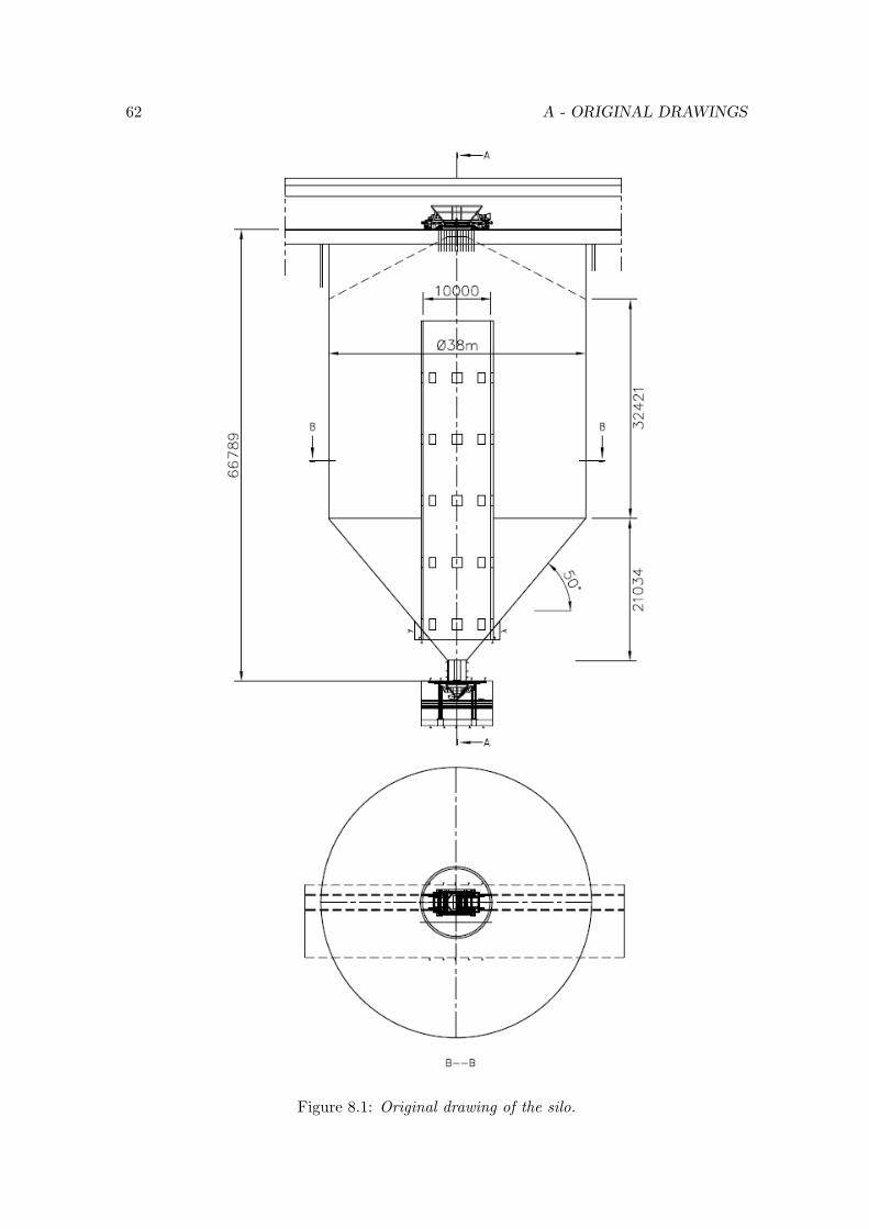
Figure 8.1: Original drawing of the silo.

63

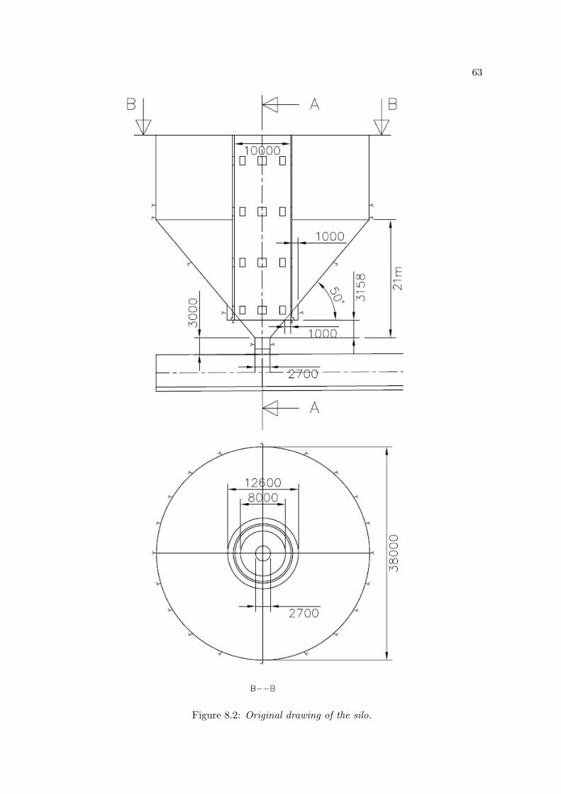
Figure 8.2: Original drawing of the silo.

64 A - ORIGINAL DRAWINGS

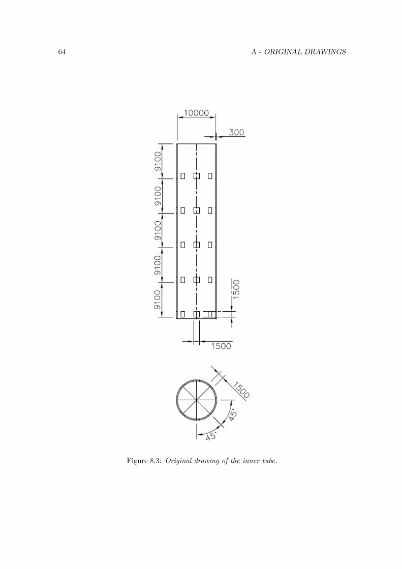
Figure 8.3: Original drawing of the inner tube.

Documents

NUMERICAL ANALYSIS OF SILO DISCHARGE - · PDF fileNUMERICAL ANALYSIS OF SILO DISCHARGE. ... To fulﬂll these two demands the original design of the silo has a perforated inner tube