NUMERICAL ANALYSIS OF SPATIAL EVOLUTION OF POWER IN AN EDFA

UNDER TEMPORAL STEADY STATE

Thesis

Submitted to

School o f Engineering UNIVERSITY OF DAYTON

In partial fulfillment o f the requirement for the degree o f

Master o f Science in Electrical Engineering

By

Mrudula N Garagaparti

School o f Engineering UNIVERSITY OF DAYTON

Dayton, Ohio May 2006

NUMERICAL ANALYSIS OF SPATIAL EVOLUTION OF POWER IN AN EDFA UNDER TEMPORAL STEADY STATE

APPROVED BY:

Monish R. Chatteijee, Ph.D. Advisory Committee Chairman Professor, Department o f Electrical Engineering

Partha $. Ban^rjee, Ph.D. Committee Member Professor, Department o f Electrical Engineering

Guru Subramanyam, Ph.D. Committee Member Associate Professor, Department of Electrical Engineering

Donald L. Moon, Ph.D. Joseph ST. Salib£ Ph.D., P.E.Associate Dean Dean, School o f EngineeringGraduate Engineering Programs & Research,School o f Engineering

ii

ABSTRACT

NUMERICAL ANALYSIS OF SPATIAL EVOLUTION OF POWER IN AN EDFA UNDER TEMPORAL STEADY STATE

Name: Mrudula N. Garagaparti

Department of Electrical Engineering

University o f Dayton, May 2006

Advisor: Dr. Monish. R. Chatteijee

Erbium Doped Fiber Amplifiers (EDFA) have revolutionized long haul fiber

optic communication systems. The numerous advantages o f erbium amplifier over other

amplifiers such as semiconductor laser amplifiers, Raman amplifiers and Brillouin

amplifiers have triggered the undertaking of this work. In this work our main objective is

to set up power evolution equations for EDFAs and find solutions to these equations.

Analysis o f power distribution in EDFAs typically proceeds from two sets o f equations.

The first set o f equations depends on the spatial variations o f signal, pump and the

amplified spontaneous emission (ASE) powers. The second set shows the rate o f change

with time of population densities o f ground and metastable levels in the amplifier. In

these equations, power and number densities are coupled together, leading to a highly

nonlinear spatial - temporal system. We have used two approaches to solve these

equations. In the first approach we have solved power evolution equations numerically.

For solving rate equations numerically, we have used the model o f a three level laser

iii

system. We have simplified the problem to some extent by assuming that the populations

reach temporal steady state (with that we were originally interested in the transient

population dynamics). In the second approach we obtained analytic solution to the power

equations assuming temporal and spatial steady state o f the population densities. We have

solved the equations using both approaches, and the numerical graphs for the population

densities, signal and ASE power versus distance are plotted. It is found that there is a

region (the gain region) where the population, once inverted, remains approximately

constant which leads to amplification in the EDFA. Comparing with literature, some

physical interpretations o f the numerical findings are also summarized in this work.

IV

ACKNOWLEDGEMENTS

I sincerely thank my advisor Dr. Monish Chatteijee for his guidance, inspiration, patience

and excellent advising. Without his guidance and support I would never have made this

work possible.

I want to thank my committee members Dr. Partha Baneijee and Dr. Guru Subramanyam

for their time and patience.

I would like to thank Dr. Malcolm Daniels, Chair o f The Department o f Electrical and

Computer Engineering, for his support.

My special thanks to Arun M Venkataraman for his endless support and guidance in my

work.

I am also thankful to my husband Sekhar Kanagala and to all my friends Yoga L.

Srinivas Kantamani, Sangameshwar Sonth, Ramakrishna Gudavalli and Divya

Kanneganti. I am dedicating this work to my Beloved Parents with whose blessings I

accomplish all my endeavors.

v

TABLE OF CONTENTS

ABSTRACT iii

ACKNOWLEDGEMENTS v

LIST OF FIGURES viii

LIST OF TABLES x

CHAPTER1. INTRODUCTION

1.1 Background1.2 Historical Development of EDFA

1.2.1 Origin of Optical Amplifiers1.2.2 The Road to Fiber Amplifiers1.2.3 Work on EDFA in 80’s

1.3 EDFAs in Transmission Networks

2. CHARACTERISTICS OF FIBER BASED OPTICAL AMPLIFIERS2.1 Optical Amplifiers

2.1.1 Important Parameters of Optical Amplifiers2.1.2 Optical Amplifier Applications2.2.3 Types of Optical Amplifiers

2.2 Architecture of EDFA2.3 Characteristics o f EDFA

2.3.1 Spectroscopy of Erbium2.3.2 Gain versus Pump Power2.3.3 Gain versus Signal Power and Amplifier Saturation2.3.4 ASE Noise and Noise Figure

2.4 Four level Fiber Amplifier for 1.3/zm2.4.1 Gain in a Four Level System2.4.2 Pr3+ Doped Fiber Amplifiers2.4.3 Nd3+ Doped Fiber Amplifiers

112245 7

9991113181920 21232425262930

3. TEMPORAL AND SPATIAL EVOLUTION OF POWER IN EDFA - ANUMERICAL APPROACH 33

3.1 Introduction 333.2 Modeling of EDFA as Three level System 333.3 Quasi Analytical Solution of Power Equations 343.4 Signal and ASE Power Evolution 36

vi

4. TEMPORAL AND SPATIAL EVOLUTION OF POPULATION ANDPOWER IN EDFA - A NUMERICAL APPROACH 3 8

4.1 Introduction 384.2 Rate Equations 3 84.3 Pump Configurations 394.4 Solution for the EDFA Rate Equations - Numerical Approach 41

4.4.1 Numerical Approach 434.5 Graphical Results and Analysis 44

4.5.1 Population Inversion 464.5.2 Variation of Input Signal Power 484.5.3 Variation of Input Pump Power 524.5.4 Variation on Pump and Signal Wavelength 53

4.5.4.1 Effect o f Pump and Signal Wavelength onPopulation Inversion 56

4.6 Optimum Parameter Values 604.7 Accuracy of the Analysis and Plots 624.8 Solution for the EDFA Power Evolution Equations - Analytical

Approach 624.9 Conclusion 63

5. SUMMARY AND CONCLUSIONS 645.1 Summary 645.2 Future Work 65

vii

L IS T O F F IG U R E S

2.1 Four possible applications o f optical amplifiers in lightwave systems; inlineamplifiers, booster amplifier, preamplifier, compensation o f distribution losses in LAN 13

2.2 The energy level scheme associated with SRS 15

2.3 Architecture o f an EDFA implementation 18

2.4 Energy level diagram of Er:glass showing absorption and radiativeTransitions 20

2.5 Absorption spectrum of alumino silicate Er3+:doped fiber 21

2.6 Signal gain at X = 1.531 fim versus input pump power at X = 514nm fordifferent fiber lengths 22

2.7 Schematic representation of ASE 25

2.8 Four level system used for the amplifier model 26

2.9 Population inversion in an ideal system 27

2.10 Energy level diagram of Praseodymium showing the 1,3/zm transition 29

2.11 Energy level diagram of Neodymium and the relative transition for1,3/tm for the amplification process 31

2.12 Gain at 1.3/tm and fluorescence as a function of pump power in an Nddoped fluoride fiber amplifier 32

3.1 Three Level Laser Energy Level Diagram 34

3.2 ASE evolution along the fiber length using Franco’s Equations 37

3.3 Signal Power evolution along the fiber amplifier length using Franco’sEquations 37

4.1 (a) Copropagating Pump and Signal 40

viii

(b) Counter Propagating Pump and Signal 40

(c) Bidirectional Pump 41-124.2 (a) Evolution of Signal, Pump and ASE power for initial ASE as 10'

Watts 44

(b) Evolution o f Signal, Pump and ASE power for initial ASE as 10'15Watts 45

4.3 (a) Population Evolution of Ground level (Ni) and Metastable level (N2)in an EDFA 46

(b) Gain Plot for EDFA 46

4.4 Population Inversion for Different Population Densities 47

4.5 Variation of Output Signal Power for Different Input Signal Powers 48

4.6 Gain Plot for Different Input Signal Powers 49

4.7 Variation of Pump Power for Different Input Signal Powers 50

4.8 (a) Population Inversion for Input Signal Power 1 mW 51

(b) Population Inversion for Input Signal Power 1 OmW 51

4.9 (a) Population Inversion for Input Pump Power 1 OmW 52

(b) Population Inversion for Input Pump Power 50mW 53

4.10 (a) Variation of Output Signal Power for Different Pump Wavelengths 53

(b) Variation o f Pump Power for Different Pump Wavelengths 54

4.11 (a) Variation o f Output Signal Power for Different Signal Wavelengths 55

(b) Variation of Pump Power for Different Signal Wavelengths 55

4.12 (a) Population Inversion for Pump Wavelength 1480nm 56

(b) Population Inversion for Pump Wavelength 151 Onm 57

(c) Population Inversion for Pump Wavelength 1550nm 57

4.13 (a) Population Inversion for Signal Wavelength 1400nm 58

(b) Population Inversion for Signal Wavelength 1530nm 59

(c) Population Inversion for Signal Wavelength 1600nm 59

ix

4.14 Population Inversion for N t = 5 x l0 18 and Input Pump 50mW

4.15 Population Inversion for N, = 8x 1018 and Input Pump 50mW

61

61

x

LIST OF TABLES

2.1 Summary of the advantages and disadvantages of different types o f amplifiers....... 18

3.1 Values of the Parameters used to Generate Franco P lo ts ..............................................37

4.1 Fiber Amplifier Parameters used in Calculations...........................................................43

4.2 Pump and Signal Powers for different Az at z = 30m.................................................... 62

xi

CHAPTER 1

INTRODUCTION

1.1 Background:

The erbium doped fiber amplifier is emerging as a major enabler in the

development o f world wide fiber optic networks. The emergence of the fiber amplifier

foreshadows the invention and development o f novel guided wave devices that should

play a major role in the continuing increase in transmission capacity and functionality of

fiber networks. Currently fiber networks are used predominantly in long distance

telephone networks, high density metropolitan areas and in cable television trunk lines.

The most vivid illustrations o f fiber based transmission systems have been in undersea

transcontinental cables [24].

The technique o f new light wave amplification in situ with vastly improved

capacity and cost is based on the recent development o f erbium doped fiber amplifiers.

Undersea systems were the early beneficiaries, as EDFA repeaters replaced expensive

and intrinsically unreliable electronic regenerators. Indeed, early EDFA technology was

driven by the submarine system developers who were quick to recognize its advantages

soon after the first diode pumped EDFA was demonstrated in 1989 [25]. Terrestrial

telecommunications systems have also adopted EDFA technology in order to avoid

electronic regeneration. Hybrid fiber/coax cable television networks employ EDFAs to

extend the number o f homes served. An equally attractive feature o f the EDFA is its wide

1

gain bandwidth product. Along with providing gain at 1550nm in the low loss window of

silica fiber it can provide gain over a band that is more than 4000 GHz wide. With

available wavelength division multiplexing components, commercial systems transport

more than 16 channels on a single fiber; the number is expected to reach 100 within the

next decade. Hence, installed systems can be upgraded many fold and new WDM

systems can be built inexpensively with much greater capacity.

The erbium amplifier is a three level system as opposed to neodymium, which is

a four level system. One significant difference between the two types is that a good deal

o f more pump power is required to invert the three level system. Hence, neodymium ions

were the earliest successful rare earth dopant used in lasers. However, erbium is the more

popular choice for fiber dopant because the amplifiers with using this dopant were having

high gain and efficiency.

1.2 Historical Development of EDFAs

1.2.1 Origin of optical amplifiers

Optical amplifiers play an exceptionally important role in long haul networks.

Prior to the advent o f optical amplifiers, the standard way o f coping with the attenuation

o f light signals along a fiber span was to periodically space electronic regenerators along

the line [24], Such regenerators consist o f a photodetector to detect the weak incoming

light, electronic amplifiers, timing circuitry to maintain the timing o f the signals, and a

laser along with its driver to launch the signal along the next span. Such regenerators are

limited by the speed of their electronic components. Thus even though fiber systems have

inherently large transmission capacity and bandwidth due to their optical nature, they are

limited by electronic regenerators in the event such regenerators are employed. The cost

and complexity o f converting the signal to electronic form in electro optic repeaters, and

the associated reduction in speed of operation, created the need for optical amplifiers.

Optical amplification is based on stimulated emission. Early laser developers saw

amplification via stimulated emission as a step toward building a laser. As opposed to

standard electronic repeaters and amplifiers, optical fiber amplifiers are purely optical in

nature, and require no high speed circuitry. The signal is not detected and regenerated;

rather, it is very simply optically amplified in strength by several orders of magnitude as

it traverses the active region of the amplifier in situ, without being limited by any

electronic bandwidth. The shift from regenerators to amplifiers thus permits a dramatic

increase in the capacity and speed of the transmission system, and this feature is being

realized in current applications.

The basic concept of a traveling wave optical amplifier was first introduced in

1962 by Geusic and Scovil [1]. Shortly thereafter, an optical fiber amplifier was invented

in 1964 by E.Snitzer, then at the American Optical Corporation, who described an unclad

neodymium glass fiber amplifier at 1.06 pm. Snitzer later, demonstrated an amplifier in a

clad fiber. This work lay dormant for many years thereafter. It emerged as an exceedingly

relevant technological innovation after the advent o f silica glass fibers for

telecommunications. Motivation for developing optical amplifiers prior to the emergence

of fiber optic communications was virtually non-existent, except for a few optical

amplifiers built to raise pulse powers to very high levels, there was no need for optical

amplifiers until the advent of fiber optic communications. One approach was to develop

amplifiers from semiconductor lasers used as light sources. Semiconductors have high

gain, so suppressing reflection from the end facets of the chip looked attractive.

3

Stimulated Raman scattering also looked promising because although it required very

high pump power, it could be distributed along the entire length of a fiber. Eventually,

EDFAs effectively replaced semiconductor optical amplifiers and Raman amplifiers,

since the latter suffer serious technical problems.

Snitzer also demonstrated the first erbium doped glass laser [2]. This work

represents the earliest fiber laser. Interestingly, rare earth doped lasers in a small diameter

crystal fiber form were investigated during the early 70s as potential devices for fiber

transmission systems [3]. The crystal fibers had cores as small as 15 pm in diameter, with

typical values in the 25 pm to 70 pm range. The crystalline cores were doped with

neodymium, surrounded by a fused silica cladding. Lasing o f this device was achieved at

1.06 pm. Since commercial fiber-optic transmission systems did not adopt the 1.06 pm

wavelength as a signal wavelength, these lasers did not make their way into today’s fiber

communication systems. The development o f low loss single mode fiber lasers was

followed by that o f fiber amplifiers.

1.2.2 The road to fiber amplifiers

The roots of erbium doped fiber lasers and amplifiers began in 1964 with the first

amplification experiments in rare earth doped fiber lasers.

When David Payne of the University of Southampton started down the road to

erbium fiber amplifiers, he was looking for fiber lasers or fiber optic sensors. In 1985, he

recognized that the next thing to do is to put some rare earths into the fibers. They started

with neodymium, the best developed solid state laser dopant. They found that the rare

earth ions caused no significant losses at the low doping levels they used [9]. The next

step was to make a fiber laser. Payne et.al noted that doped fibers could be used to make

4

an optical amplifier. Solid state lasers had too little gain to provide the 30 dB

amplification needed in fiber optic systems. Instead, fiber lasers were experimented with,

since power could build with in a resonant cavity. However, fiber lasers were typically

several meters in length - long by conventional laser standards.

As indicated before, rare earth elements were already well known as lasers in bulk

glass and crystalline hosts. Though the late 1970s and early 1980s, researchers used

neodymium, thulium and ytterbium before erbium, noting that the neodymium laser

could be tuned across 80nm, while the erbium laser only across 25nm [10].

It turns out that the three level erbium system absorbs strongly around the laser

transition at low pump powers and the 1530nm Er transition wavelength is also well

adapted to propagation in silica fibers. The Southampton group developed the first

amplifier in late 1986; the peak gain was 26 dB at 1536 nm in a three meter fiber,

pumped at 514.5 nm by a mode locked argon laser [11], Later, by switching to pumping

with a mode locked argon pumped dye laser near 670nm, a peak gain of 28dB was

achieved, along with a gain of at least 10 dB between 1530 and 1555nm.

1.2.3 Work on EDFA in 80s

Emmanuel Desurvire and coworkers in 1986 started working on erbium fibers at

Bell Laboratories. They built an erbium fiber amplifier, pumping with a continuous wave

argon laser at 514.5nm, and developed a theoretical model, optimizing thereby the

effective fiber length[28]. The need for a better pump source remained a major issue.

Argon lasers used in the laboratory, required 100s o f kilowatts o f electricity, cooling

water and extensive care, often left as assignment to laboratory assistants. Scientists

searched the erbium absorption spectrum for pump bands. British Telecom first pumped

5

an erbium fiber laser at 808nm with a dye laser [12]; The Southampton group later

pumped one with a continuous wave 8O8nm diode laser generating output to 130

microwatts [13]. A high power diode array pump at 800nm increased the laser output.

However, pumping with diode arrays at 800nm proved to be inefficient. The excited state

absorption was at least as large as ground state absorption for pumping at 810 and

488nm. Excited state absorption was found to be absent at 980nm pumping [14]; however

a diode oscillator at 980nm was not available. In 1988 Snitzer attempted operation at

1480nm. A net gain was reported when pumping erbium fiber amplifier with a color

center laser at 1490 and 1500nm [5], Eventually, 1480nm was shown to be the best

wavelength choice for the pump. The following year, Desurvire et.al demonstrated 37 dB

of gain or a record 2.1 dB per milliwatt of pump power [15]. In late 1989, the Nakazawa

group of Japan reached a 46.5 dB gain when pumping an erbium fiber amplifier with

133mW from multiple 1480 nm diode lasers [16]. Diode pumping had compelling

advantages for practical fiber amplifiers, and development quickly narrowed to systems

pumped at 980nm and 1480nm. The longer wavelength got a headstart because 1480nm

lasers were better developed. A decade later, these two wavelengths remain the standard

choices today.

Erbium doped fiber amplifiers for traveling wave amplification of 1.5 pm signals

were simultaneously developed in 1987 at the University o f Southampton and at AT&T

Bell Laboratories [11]. A key advance was the recognition that the Er3+ ion, with its

propitious transition at 1.5 pm was ideally suited as an amplifying medium for modem

fiber optic transmission systems at 1.5 pm. The high signal gains obtained with these

erbium doped fibers attracted worldwide attention. As the previously mentioned amplifier

6

demonstrations typically used large frame laser pumps, the final hurdle was to

demonstrate an effective erbium doped fiber amplifier pumped by a laser diode or an

array. This was achieved in 1989 by Nakazawa and coworkers, after the demonstration

by Snitzer et.al., that 1.48 pm was a suitable pump wavelength for erbium amplification

in the 1.53 pm to 1.55 pm range[5]. Nakazawa and group were able to use high power

1.48 pm laser diode pumps previously developed for fiber Raman amplifiers[6]. This

demonstration opened the way to serious consideration of amplifiers for systems

application. Previous work exploring optical amplification with semiconductor amplifiers

provided a foundation for understanding signal and noise issues in optically amplified

transmission systems [7].

1.3 EDFAs in Transmission Networks:

Starting in 1989, erbium doped fiber amplifiers were the catalyst for an entirely

new generation of high capacity undersea and terrestrial fiber optic links and networks.

At an optical fiber conference in 1989, Desurvire’s group reported that erbium fiber

amplifiers could handle signals at multiple wavelengths without crosstalk between

channels [17]. By inserting a fiber amplifier after the first 51 km o f fiber, researchers at

Bellcore stretched the transmission distance to 93.7km, claiming a record for the bit rate

distance product for a single amplifier. Bellcore also demonstrated 16 channel

wavelength division multiplexing(WDM), using coherent transmission without optical

amplifiers and transmitting only 155Mbit/s on each channel [18]. A team from KDD

R&D laboratories transmitted 2.4 Gbit/s at four separate wavelengths about 2nm apart

through 459 km of fiber using six erbium amplifiers along the route [19]. The first

undersea test of erbium doped fiber amplifiers in a fiber optic transmission cable

7

occurred in 1989[8]. By 1996 erbium doped fiber amplifiers were in commercial use in a

number o f undersea links increasing the capacity near ten fold over the previous

generation o f cables.

The first implementation of erbium doped fiber amplifiers has been in long haul

systems such as the TAT-12, 13 fiber cable that AT&T and its European partners

installed across the Atlantic in 1996 [24]. This cable, the first transoceanic cable to use

fiber amplifiers, provides a near ten fold increase in voice and data transmission capacity

over the previous transatlantic cable.

With recent advances made throughout the 1990s in a number o f optical

transmission technologies, be it lasers or novel components such as fiber grating devices

or signal processing fiber devices, the optical amplifier offers a solution to the high

capacity needs o f today’s voice and data transmission applications. Commercial erbium

fiber amplifiers are finding increasing applications, along with steady improvements in

the technology. Today, erbium fiber amplifiers carry signals thousands o f kilometers in

submarine cables and transmit dozens of channels at lOGbit/s in commercial land

systems [25]. Developers opened up a new erbium fiber window at 1570 to 1620 nm,

where gain is lower but still adequate for optical amplifiers. Erbium remains by far the

best fiber amplifier dopant.

8

CHAPTER 2

CHARACTERISTICS OF FIBER BASED OPTICAL AMPLIFIERS

2.1 Optical Amplifiers

As discussed in the previous chapter, the transmission distance o f any fiber optic

communication system is limited by fiber loss and dispersion. Optical amplifiers in fibers

amplify the incident light through stimulated emission, the same mechanism used by

lasers. The external pump, either optically or electronically, generates a population

inversion in amplification media. Indeed, an optical amplifier is nothing but a laser

without feedback, where an amplified photon is a signal photon.

2.1.1 Important Parameters of Optical Amplifiers:

Gain (dB):

An important measure for the amplification ability o f an optical amplifier is the

optical gain realized when the amplifier is pumped to achieve population inversion. The

optical gain in general depends not only on the frequency o f the incident signal, but also

on the local beam intensity at any point inside the amplifier. In optical amplifiers, gain is

defined as the ratio o f output to input optical power and is usually expressed in dB

through

Gain (dB) = 10 x logio[Pout/ Pm]

(2T)

9

Gain saturation:

When the optical power is too high, the gain coefficient starts to decrease, thus

reducing the power o f the signal undergoing amplification. This effect is called gain

saturation. More precisely, when the optical power P exceeds the saturation optical power

Psat, the gain becomes saturated. Gain saturation is an important characteristic to

determine the saturated output power.

Saturated output power:

It is the maximum output power Pout from an optical amplifier when the optical

power within the amplification medium reaches the saturation optical power Psat. The

saturated output power Pout is usually less than the saturation optical power Psat because

the latter is the sum of the input pump power and output power.

Amplified Spontaneous Emission (ASE):

It is the amplified optical power resulting from the spontaneous (i.e., not

stimulated by any signal photons) release o f photons within the gain spectrum of an

EDFA operation due to the random decay of erbium ions from the metastable state to the

ground state. A detailed description of the occurrence and effects o f ASE is given at a

later stage in this chapter.

Noise Figure (dB):

It quantifies the noise performance o f an optical amplifier and is defined as the

signal-to-noise ratios o f the input and output signals:

nf= [SNR]in/[SNR]0Ut

(2.2)

It is usually expressed in units o f dB, given by

10

NF= 10 x lo g w tf S N R M S N R M

(2-3)

NF is often referred to as a figure o f merit when one is evaluating the noise performance

o f an optical amplifier. The SNR degradation is quantified through this parameter.

Small Signal Gain (dB):

It is the amplifier gain, when operated in the linear region, where it is essentially

independent o f the input signal power at a specific signal wavelength and operating

conditions (e.g., pump power, temperature ...).

2.1.2 Optical Amplifier Applications

Optical amplifiers can serve several purposes in the design o f fiber optic

communication systems. Four such applications are as follows [23],

Inline amplifiers:

When optical amplifiers are used to replace electronic regenerators as shown in

Fig 2.1(a) in long haul systems, they are called in-line amplifiers. They modify a small

input signal and boost it for retransmission down the fiber. Controlling the small signal

performance and noise added by the EDFA reduces the risk o f limiting a system’s length

due to the noise produced by the amplifying components. Such a replacement can be

carried out as long as the system performance is not limited by the cumulative effects of

dispersion and spontaneous emission.

11

Power amplifiers:

Optical amplifiers can also be used to increase the transmitter power by placing

them just after the transmitter as shown in Fig 2.1(b). Such amplifiers are called power

amplifiers or boosters. This application requires the amplifier to take a large signal input

and provide the maximum output level. Small signal response is not as important because

the direct transmitter output is usually -10 dBm or higher. The noise added by the

amplifier at this point is also not as critical because the incoming signal has a large

signal-to-noise ratio (SNR).

Preamplifiers:

In the past, receiver sensitivity o f -30 dBm at 622 Mb/s was acceptable; however,

currently, the demands require sensitivities o f -40 dBm or -45 dBm. This performance

can be achieved by placing an optical amplifier prior to the receiver which is shown in

the Fig 2.1(c). Boosting the signal at this point presents a much larger signal into the

receiver, thus easing the demands of the receiver design. This application requires careful

attention to the noise added by the amplifier; the noise added by the amplifier must be

minimal to maximize the received SNR.

LAN amplifier:

Another application of optical amplifiers is to use them for compensating

distribution losses in local area networks (LANs) [29]. Such amplifiers are called LAN

amplifiers and they are depicted in the Fig 2.1(d).

12

Fig. 2.1: Four possible applications o f optical amplifiers in lightwave systems; (a) inline amplifiers,(b) booster amplifier,(c) preamplifier and (d) compensation o f distribution losses in LAN [23].

2.1.3 Types of Optical Amplifiers

A number of different types of optical amplifiers have been studied [26]. These

include:

• semiconductor laser amplifiers (SLA),

• fiber Raman amplifiers,

• fiber Brillouin amplifiers, and

• rare earth ion doped fiber amplifiers.

13

Semiconductor laser amplifiers:

SLAs provide high gain, large bandwidth, and lower current consumption with a

high expected reliability and small size. SLAs are bidirectional amplifiers and can be

used only as lumped amplifiers. Disadvantages o f SLAs as compared to erbium

amplifiers involve the interference between the adjacent pulses in the saturation regime

due to the short gain recovery time. The short gain recovery time allows the amplification

condition of a given pulse to affect only a relatively small number o f the following time

slots which results in a pulse pattern dependent intersymbol interference. This limits the

maximum bit rate and reduces the acceptable input power. SLAs produce a significant

pulse pattern distortion in the output signal at 25Gbps where no significant degradation

was observed with erbium amplifiers over lOOGbps [30]. An additional disadvantage of

SLAs is a large coupling loss between the SLA and the optical fiber. The losses degrade

both the fiber to fiber gain and the effective noise figure. Losses can reach up to lOdB

[31]. In view o f the above, rare earth activated fibers find a major field of application as

traveling wave fiber amplifiers for optical communications as an alternative to

semiconductor laser amplifiers.

Raman amplifiers (RAs):

A fiber Raman amplifier uses stimulated Raman scattering (SRS) occurring in

silica fibers when an intense pump beam propagates through it [32], SRS differs from

standard stimulated emission in one fundamental aspect: whereas in the case o f standard

stimulated emission, an incident photon stimulates the emission of another identical

photon without losing its energy, in the case of SRS the incident pump photon loses its

energy to create another photon of reduced energy at a lower frequency, the remaining

14

energy is absorbed by the medium in the form of molecular vibrations. Thus Raman

amplifiers must be pumped optically to provide gain in contrast with SLAs which can be

pumped electronically. An important difference from the case o f SLA is that population

inversion is not required for fiber Raman amplifiers. In fact, SRS is a nonresonant

nonlinear phenomenon that does not require population transfer between energy levels.

The Fig.2.2 shows schematically the operation o f fiber Raman amplifiers and the energy

Fig. 2.2: The energy level scheme associated with SRS [23].

The pump and signal beam at frequencies <ap and cos are injected into the fiber

through a wavelength selective coupler. The energy is transferred from the pump beam to

the signal beam through SRS as the two beams copropagate along the fiber. The pump

and signal beams can also be injected in such a way that they counter propagate inside the

fiber.

Both Raman amplifiers and erbium amplifiers amplify optical signals in the fiber

by transferring energy from a pump to the signal. RAs have a low noise figure, low

15

connection loss, high gain, high output power, and broad bandwidth. The major drawback

o f RA’s as compared to erbium amplifiers is their low efficiency (8dB fiber loss

compensated with a lOOmW pump power in an 80km fiber) [33].

Brillouin amplifiers (BAs):

Fiber Brillouin amplifiers are also pumped optically and a part of the pump power

is transferred to the signal through SBS (stimulated Brillouin scattering). BAs are

different from RAs in that the difference between the pump and signal frequencies is

much smaller. The amplification process is similar and called stimulated Brillouin

scattering. BAs provide high gain, high efficiency, and low connection loss. The major

disadvantages are narrow bandwidths required for the pump signal, a large noise figure

due to the thermal noise, and a low output power [34],

Both the Raman scattering and the Brillouin scattering are examples of inelastic

scattering during which the frequency of the scattered light is shifted downward. Both of

them can be understood as scattering of a photon to a lower energy photon such that the

energy difference appears in the form of a phonon. The main difference between the two

is that optical phonons participate in Raman scattering whereas acoustic phonons

participate in Brillouin scattering. SBS also differs from SRS in the aspect that the

amplification occurs only when the signal beam propagates in a direction opposite to that

of the pump beam. Both scattering processes result in a loss of energy at the incident

frequency and constitute a loss mechanism for optical fibers. However, the scattering

cross sections are sufficiently small that power loss is negligible at low power levels. At

higher power levels the nonlinear phenomena o f stimulated Raman scattering and

stimulated Brillouin scattering can lead to considerable fiber loss.

16

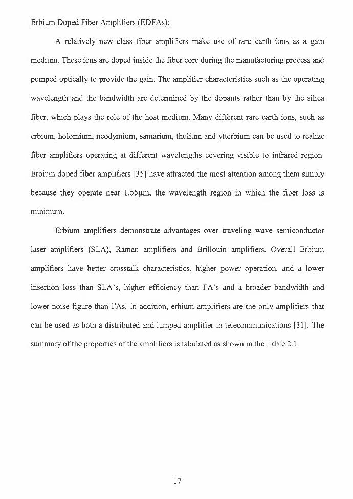
Erbium Doped Fiber Amplifiers (EPFAs):

A relatively new class fiber amplifiers make use o f rare earth ions as a gain

medium. These ions are doped inside the fiber core during the manufacturing process and

pumped optically to provide the gain. The amplifier characteristics such as the operating

wavelength and the bandwidth are determined by the dopants rather than by the silica

fiber, which plays the role of the host medium. Many different rare earth ions, such as

erbium, holomium, neodymium, samarium, thulium and ytterbium can be used to realize

fiber amplifiers operating at different wavelengths covering visible to infrared region.

Erbium doped fiber amplifiers [35] have attracted the most attention among them simply

because they operate near 1.55pm, the wavelength region in which the fiber loss is

minimum.

Erbium amplifiers demonstrate advantages over traveling wave semiconductor

laser amplifiers (SLA), Raman amplifiers and Brillouin amplifiers. Overall Erbium

amplifiers have better crosstalk characteristics, higher power operation, and a lower

insertion loss than SLA’s, higher efficiency than FA’s and a broader bandwidth and

lower noise figure than FAs. In addition, erbium amplifiers are the only amplifiers that

can be used as both a distributed and lumped amplifier in telecommunications [31]. The

summary o f the properties o f the amplifiers is tabulated as shown in the Table 2.1.

17

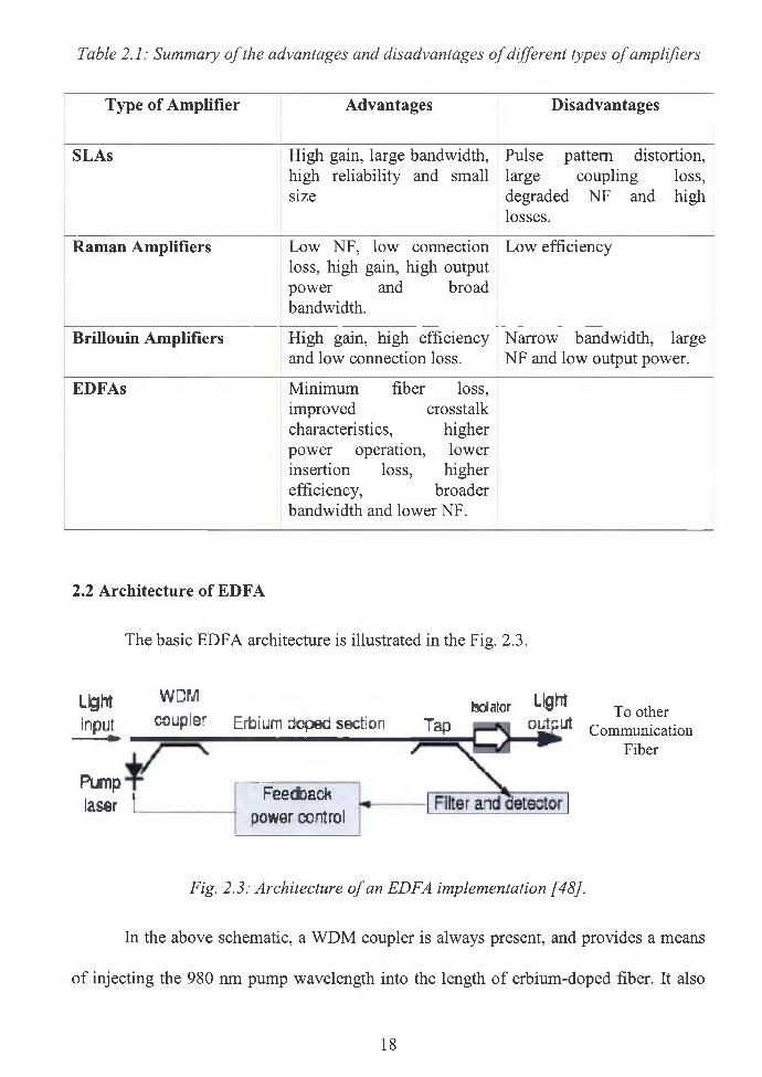
Table 2.1: Summary o f the advantages and disadvantages o f different types o f amplifiers

Type of Amplifier Advantages Disadvantages

SLAs High gain, large bandwidth, high reliability and small size

Pulse pattern distortion, large coupling loss,degraded NF and high losses.

Raman Amplifiers Low NF, low connection loss, high gain, high output power and broadbandwidth.

Low efficiency

Brillouin Amplifiers High gain, high efficiency and low connection loss.

Narrow bandwidth, large NF and low output power.

EDFAs Minimum fiber loss,improved crosstalkcharacteristics, higherpower operation, lower insertion loss, higherefficiency, broaderbandwidth and lower NF.

2.2 Architecture of EDFA

The basic EDFA architecture is illustrated in the Fig. 2.3.

Lightinput

WDMcoupler Erbium doped section Tap

Pump laser t Feedback

power control

Isolator Light output

Fig. 2.3: Architecture o f an EDFA implementation [48].

To other Communication

Fiber

In the above schematic, a WDM coupler is always present, and provides a means

o f injecting the 980 nm pump wavelength into the length o f erbium-doped fiber. It also

18

allows the optical input signal to be coupled into the erbium-doped fiber with minimal

optical loss. The erbium-doped optical fiber is usually tens o f meters long. The 980 nm

energy pumps the erbium atom into a slowly decaying, excited state. When energy in the

1550 nm band travels through the fiber it causes stimulated emission of radiation, much

like in a laser, allowing the 1550 nm signal to gain strength. The erbium fiber has

relatively high optical loss, so its length is optimized to provide maximum power output

in the desired 1550 nm band [24], The tap that goes to detector is used to monitor the

optical output power. The optical isolator is placed to monitor reflections back into the

EDFA. This feature can be used to detect if the connector on the optical output has been

disconnected. All these components have single mode fiber pigtails and are spliced

together.

2.3 Characteristics of EDFA

The characteristics o f an EDFA are essentially determined by the amplifier gain,

saturation, and noise properties; all three are generally coupled together. Ideally, the

EDFA should yield the highest gain possible, while having the highest saturation output

power and lowest noise possible. The combined EDFA characteristics o f gain, saturation

power and noise are often referred as the EDFA performance. The spectroscopy o f Er

doped glass fibers plays a fundamental role in the analysis and physical understanding of

optical fiber amplifiers. All the important device characteristics o f EDFA may be

evaluated via spectroscopic properties.

19

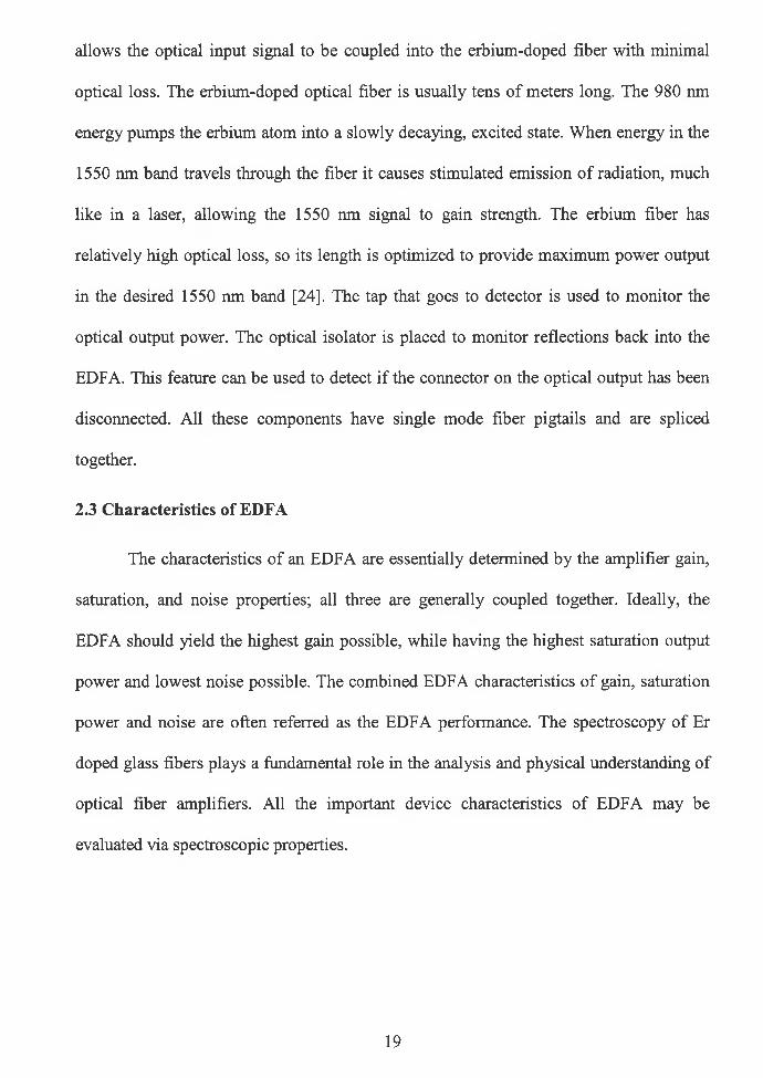
2.3.1 Spectroscopy of Erbium:

The energy levels corresponding to each possible atomic state for Er: glass are

shown in the Fig. 2.4 [27]. The figure also shows possible absorption transitions in the

visible and near infrared as well as possible radiative transitions. It shows the transition

with center wavelength o f 1.540nm, relevant to optical communications, originates from

the 4Ii3/2 level and terminates in the 4115,-2 ground level. The pump absorption transition is

justified near 1.480nm when considering the Stark level substructure o f the 4Ii3/2 and

4Iis/2 levels.

Ener

gy (1

03c

Fig. 2.4: Energy level diagram o f Er: glass showing transitions [27].

3+Er is the ion of choice for lasing and amplification in the 1.5pm region, due to

its 4Ii3/2 4Ii5/2 transition. The various absorption bands seen in this spectrum correspond

20

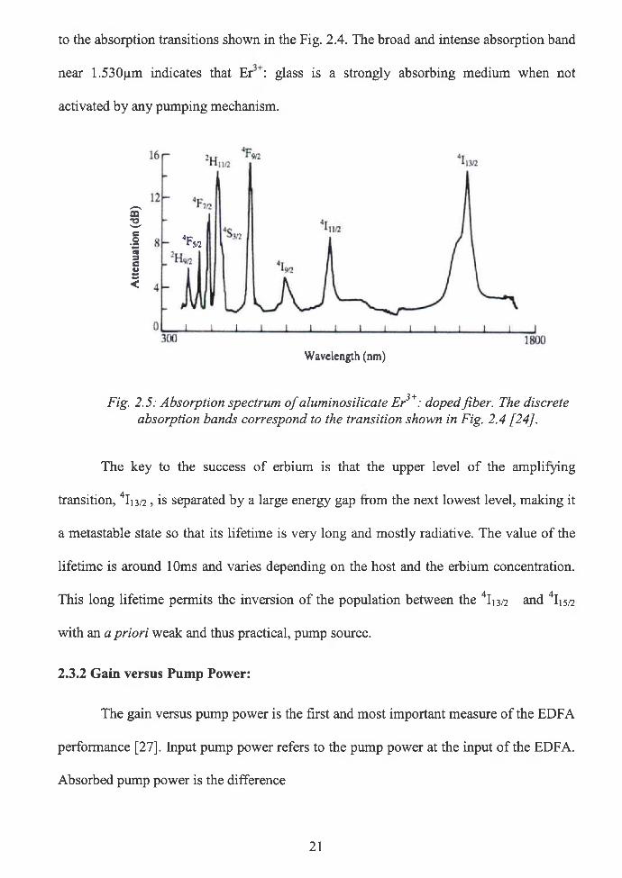
to the absorption transitions shown in the Fig. 2.4. The broad and intense absorption band

near 1.530pm indicates that Er : glass is a strongly absorbing medium when not

activated by any pumping mechanism.

Fig. 2.5: Absorption spectrum o f aluminosilicate Er3+: doped fiber. The discrete absorption bands correspond to the transition shown in Fig. 2.4 [24].

The key to the success o f erbium is that the upper level o f the amplifying

transition, 4Ii3/2, is separated by a large energy gap from the next lowest level, making it

a metastable state so that its lifetime is very long and mostly radiative. The value o f the

lifetime is around 10ms and varies depending on the host and the erbium concentration.

This long lifetime permits the inversion o f the population between the 4Ii 3/2 and 4Iis/2

with an a priori weak and thus practical, pump source.

2.3.2 Gain versus Pump Power:

The gain versus pump power is the first and most important measure o f the EDFA

performance [27]. Input pump power refers to the pump power at the input o f the EDFA.

Absorbed pump power is the difference

21

p abs _ p in p out Ip - r p r p

(2.4)

For EDFAs, absorbed pump power is generally not relevant, since the amount of

unabsorbed pump power due to bleaching can be significant in some cases. Thus,

expressing the gain characteristics as a function o f absorbed pump power does not reflect

how much launched pump power is necessary to achieve the result. There exists an

optimum wave length near X = 665nm (see Fig. 2.5) for which the gain is maximized and

this corresponds to the peak absorption wavelength. But at high pumps, near 980nm and

1480nm, the gain is nearly independent of the pump wavelength and this reflects a

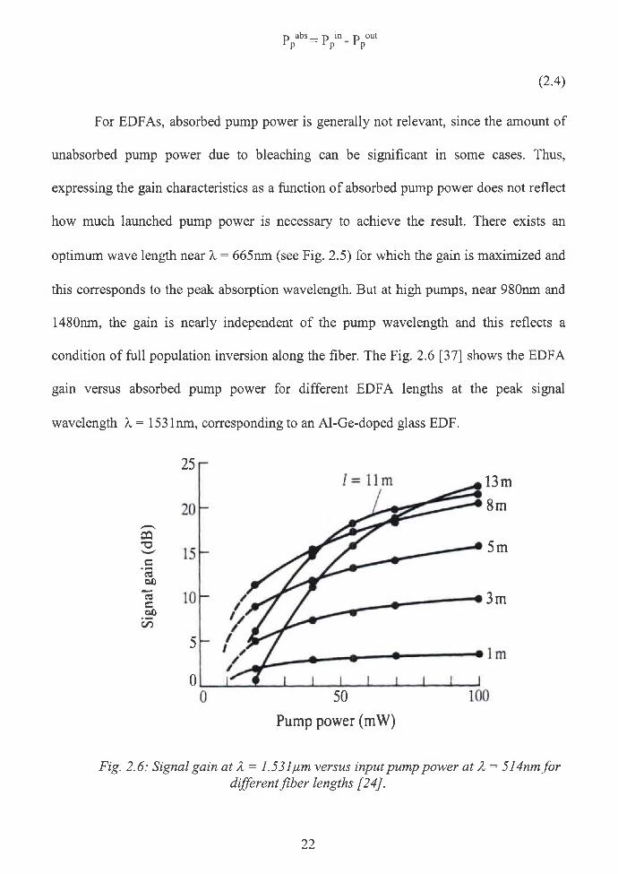
condition of full population inversion along the fiber. The Fig. 2.6 [37] shows the EDFA

gain versus absorbed pump power for different EDFA lengths at the peak signal

wavelength A = 1531nm, corresponding to an Al-Ge-doped glass EDF.

Fig. 2.6: Signal gain at 2 = 1.531pm versus input pump power at 2 = 514nm fo r different fiber lengths [24].

22

The most important feature of these measurements is the existence o f an optimum

length Lopt, different for each input pump power, for which the signal gain is maximized

for amplifier lengths L>Lopt, the signal is reabsorbed along the fiber, as a result o f an

absence o f population inversion in the fiber section, corresponding to a greater population

in the 4Ii5/2 ground level.

2.3.3 Gain versus Signal Power and Amplifier Saturation:

When EDFAs are operated in the small signal regime, the gain is independent of

the input signal power [27]. The effect of increasing the input signal power Psin on the

EDFA gain can be characterized by the expression

Psout = f(Psin) , G = f(Psm) or G = f(Ps0Ut)

(2-5)

In the small signal regime these expressions are linear.

Psout (P™) = const, x Psin, GOP” ) = G (Psout) = const.

(2-6)

Gain saturation is reached when the EDFA characteristics depart from those linear

relations. The powers are expressed in decibel - mW or dBm units, according to the

definition

P(dBm) = 10 logio [P(mW)/Po], with Po = lmW.

(2.7)

Another parameter in EDFA, which is the saturation output power Psatout; is

defined as the output power for which the EDFA gain has dropped by -3dB below its

23

unsaturated value Gmax. The power Psatout is also referred to as saturated output power for

3dB gain compression. The parameter Psat'n which is input saturation power is defined as

for which the gain saturation or compression is -3dB. The two parameter set Gmax and

Psatin or Psat°ut which corresponds to a given or available LD pump power determine the

EDFA power dynamic range. Psatout should not be confused with the EDFA saturated

output power defined as the maximum output signal power that can be achieved under

given experimental conditions. EDFAs that are operated in the saturation regime in order

to yield a maximized output signal power are referred to as power amplifiers. For power

EDFAs the power conversion efficiency is defined as the ratio

PCE = (Psout-P sin) /P p m

(2-8)

2.3.4 ASE Noise and Noise Figure:

The amplified spontaneous emission and the optical noise figure comprise the

third most important characteristic feautures o f EDFAs. The ASE power spectrum

provides useful information on the EDFA operating characteristics in various pump and

signal power regimes. The NF represents a measure of the SNR degradation from the

input to the output of the amplifier. System applications require that a certain level of

SNR be achieved at the receiver end. The ASE noise falling into the operating signal

bandwidth represents a major parameter according to which the overall system

performance can be determined.

24

Amplified spontaneous emission (ASE):

ASE arises from the fact that all the excited ions can spontaneously relax from the

upper state to the ground state by emitting a photon that is uncorrelated with the signal

photons. As shown in Fig 2. this spontaneously emitted photon can be amplified as it

travels along the fiber and stimulates the emission of more photons from excited ions,

viz., photons that belong to the same mode o f the electromagnetic field as the original

spontaneous photon. This parasitic process which can occur at any frequency within the

fluorescence spectrum of the amplifier transitions reduces the gain from the amplifier. It

robs photons that would otherwise participate in stimulated emission with the signal

photons. This limits the total amount o f gain available from the amplifier. Under normal

condition the probability o f spontaneous emission is higher than stimulated emission.

Random phase and frequency

Fig2.7: Schematic representation o f ASE [48],

2.4 Four Level Fiber Amplifier for 1.3pm

The rare earth ions that have been used for the optical amplifiers for 1.3 pm signal

wavelength all operate on the four level laser principle. The two principal candidates are

Praseodymium (Pr3+) and Neodymium (Nd3+) all doped in a nonsilica host [24]. Pr3+ has

received the most attention among the two ions. But these ions have low efficiency when

compared to the EDFA and this necessitates higher pump levels for these amplifiers.

25

Another factor is the need for fluoride fiber processing and fabrication technology, which

is less widespread and more complex than that o f silica fibers.

2.4.1 Gain in a Four Level System:

The fundamental differences between the PDF A, NDFA and the EDFA arise

because o f the differences in the gain process between a four level amplifier and a three

level amplifier.

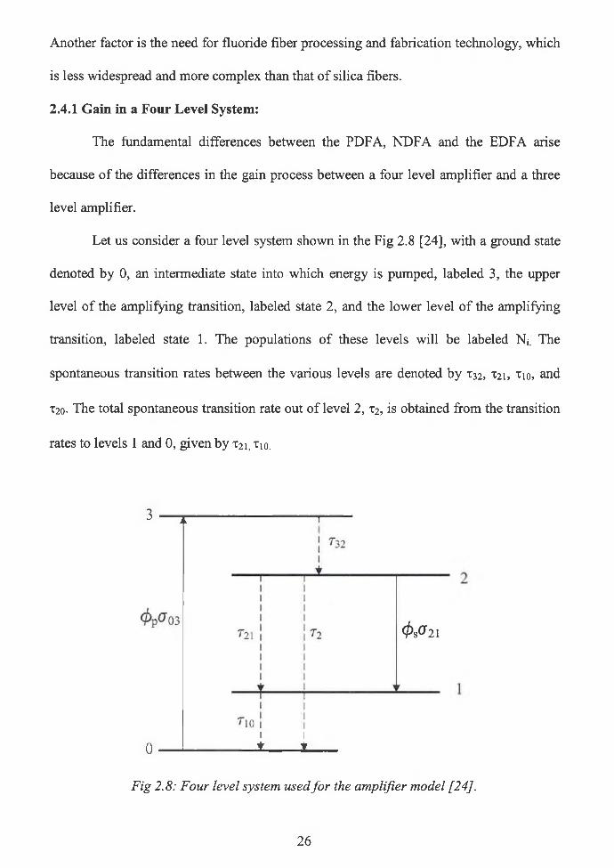
Let us consider a four level system shown in the Fig 2.8 [24], with a ground state

denoted by 0, an intermediate state into which energy is pumped, labeled 3, the upper

level o f the amplifying transition, labeled state 2, and the lower level o f the amplifying

transition, labeled state 1. The populations of these levels will be labeled Nj. The

spontaneous transition rates between the various levels are denoted by T32, T21, X10, and

T2o- The total spontaneous transition rate out o f level 2, x2, is obtained from the transition

rates to levels 1 and 0, given by T21, Tio.

3 T 7

I I± t

Fig 2.8: Four level system used fo r the amplifier model [24].

0

26

1/t32 = 1/^21+ 1/̂ 20

(2.9)

We assume a fast relaxation rate from level 3 to level 2, so that N3 ~ 0. We also assume

that level 1 empties into level 0 at a fast rate so that we can write in addition that Ni~ 0.

We then have No + N2 = N where N is the total population. For small signal gains, the

population inversion is given by

N2 ~ N2 - Ni ~ (t2 cr03 <|>p)/ ( 1 + t2 a 03 <))p)

(2-10)

In contrast to a three level system, the population inversion in a four level system is

always positive, as shown in the Fig.2.9.

Fig 2.9:Population inversion in an ideal system [24].

In the case where the pump power is zero, the signal should suffer no attenuation

and no gain. Thus, an advantage of a four level fiber amplifier as is true with Pr3+ or Nd3+

27

ions over an erbium doped fiber amplifier is that in the event o f a pump source failure the

former becomes transparent whereas the latter becomes a strong absorber. As soon as the

pump power becomes infinite, the signal experiences gain. In practice, the situation is

complicated by the fact that there is usually some nonzero background loss, such that

even with zero pump power the signal experiences some absorption in a four level

amplifier ion doped fiber. Thus a small amount o f pump power is needed to render the

active medium transparent in an EDFA. The small signal gain after the signal has

traversed a section of pumped amplifier fiber is

g — (^ e m T Pabs F)/ (ht)pAeff T|p)

(2.11)

where c em is the emission cross section, t is the upper state lifetime, ht>p is the pump

photon energy, A is the fiber core area, P abs is the absorbed pump power in the section of

fiber considered, F is the overlap integral between the pump and signal fields in the

traverse dimensions, and r)p is the fractional pump energy that propagates in the fiber core

[38]. Finally, it must be noted that for most four level fiber amplifiers, an ideal four level

system does not take into account the following complex effects

• a finite population in level 1,

• signal excited state absorptions,

• pump excited state absorption,

• competing fluorescent transitions between other levels.

2.4.2 Pr3+Doped Fiber Amplifiers:

The energy level diagram of Pr3+is shown in Fig.2.10

28

20000 “3Pi

so

toOS-4<uCW

15000 “ 'Do

10000 ” 'G 4

5000 -

3h 6

%3H4

Fig. 2.10: Energy level diagram o f Praseodymium showing the 1.3 ym transition[24].

The transition between levels ^ 4 and 3H5 is very short and there is no prospect of

obtaining sufficient population inversion on the [G4 - 3H5 transition. This is due to

nonradiative relaxation from the *G4 level to the levels directly below it, i.e. the 3F4> 3; 2

levels. This can be contrasted with the case of Er3+, where there are no intermediate levels

lying between the two levels o f the amplifying transition, eliminating the possibility for a

multitude o f nonradiative decay processes.

The Pr3+ doped fiber amplifier was first demonstrated by Ohishi and coworkers

and by other groups [39]. Gains in excess of 30dB have been observed for pump powers

on the order of several hundreds o f mW. Laser diode pumping has been demonstrated. A

gain o f 28dB was obtained when pumping with four 1.02pm laser diodes, and a one laser

29

diode pumped double pass configuration module was shown to have a gain o f 23 dB [40].

A gain o f 40dB was obtained with a two stage Pr3+ fiber amplifier with each stage

pumped by a solid state Nd: YLF laser. In a latter demonstration by the same group a

saturated signal output power o f 20dB was obtained as well as a small signal noise figure

o f 5dB, at 1,30pm [41], High gain and high output power Pr3+ fiber amplifiers using high

power MOP A laser diodes as pumps have also been demonstrated [42],

2.4.3 Nd3+Doped Fiber Amplifiers:

Nd doped fiber amplifiers were early candidates as amplifiers at 1.3 pm. But

unfortunately they suffer from a host o f problems and have never yielded suitable gains at

the wavelength of interest for transmission applications despite the fact that they can be

pumped in the 800nm region where high power laser diodes are available. But the study

of the Nd3+ based amplifiers has provided useful insights into the properties of rare earth

doped fiber amplifiers. In addition to a very strong excited state signal absorption effect,

Nd3+ suffers from the fact that another transition at a wavelength o f 1.06pm, originates

from the same 4F3/2 upper state as the 1.3 pm transition. The 1.06pm transition has, in fact

an emission cross section about four times stronger than that at 1.3 pm, and thus the

1.06 pm transition tends to steal the gain from the 1.3 pm transition. Even without these

deleterious effects, the product of the emission cross section and the lifetime for Nd3+ is

an order o f magnitude lower than that for Er3+, indicating that the pump efficiencies for

an Nd3+ fluoride fiber amplifier will be significantly lower than what we are accustomed

to for Er3+ doped fiber amplifiers at 1.5pm[43]. The Fig.2.11 shows the Nd3+ energy

levels, along with the processes relevant to gain in an Nd3+ doped amplifier.

30

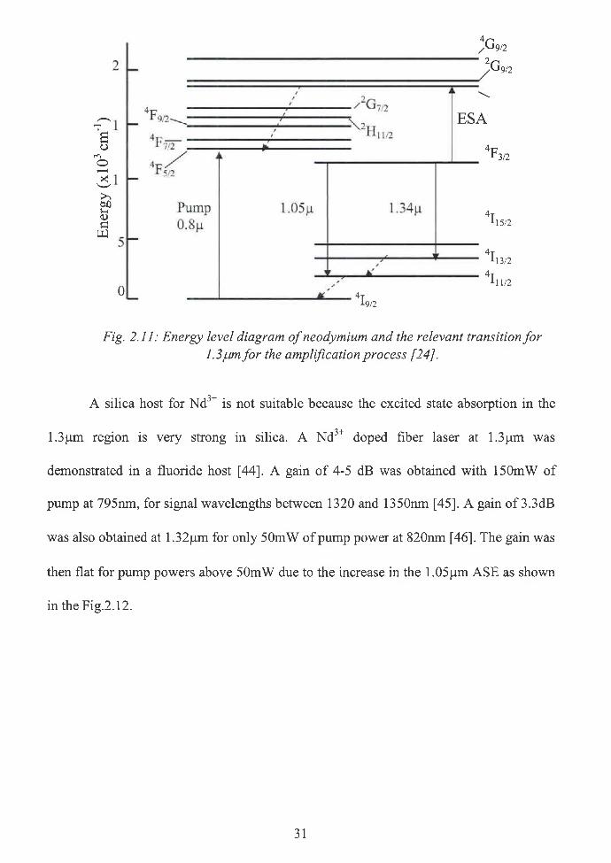
Fig. 2.11: Energy level diagram o f neodymium and the relevant transition fo r 1.3pm fo r the amplification process [24].

A silica host for Nd3+ is not suitable because the excited state absorption in the

1.3pm region is very strong in silica. A Nd3+ doped fiber laser at 1.3pm was

demonstrated in a fluoride host [44]. A gain o f 4-5 dB was obtained with 150mW of

pump at 795nm, for signal wavelengths between 1320 and 1350nm [45], A gain o f 3.3dB

was also obtained at 1.32pm for only 50mW of pump power at 820nm [46]. The gain was

then flat for pump powers above 50mW due to the increase in the 1.05pm ASE as shown

in the Fig.2.12.

31

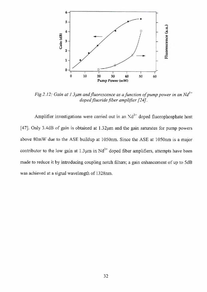
Fig.2.12: Gain at 1.3/jm and fluorescence as a function ofpump power in an Nd3+ doped fluoride fiber amplifier [24].

Amplifier investigations were carried out in an Nd3+ doped fluorophosphate host

[47]. Only 3.4dB o f gain is obtained at 1.32pm and the gain saturates for pump powers

above 80mW due to the ASE buildup at 1050nm. Since the ASE at 1050nm is a major

contributor to the low gain at 1.3 pm in Nd3+ doped fiber amplifiers, attempts have been

made to reduce it by introducing coupling notch filters; a gain enhancement o f up to 5dB

was achieved at a signal wavelength of 1328nm.

32

CHAPTER 3

SPATIAL EVOLUTION OF POWER IN EDFA

ANALYTICAL APPROACH

3.1 Introduction

The simplest treatment o f the erbium doped fiber amplifier starts out by

considering a three level atomic system [28]. Most of the important characteristics o f the

amplifier can be obtained from this simple model and its underlying assumptions. An

added complication will be stimulated emission at the pump wavelength.

As mentioned, the erbium doped amplifier is modeled as a three level laser

system. This model allows us to characterize the amplifier in terms of pump, signal and

amplified spontaneous emission (ASE) powers [24]. The rate equations describing the

effects o f pump, signal and ASE powers on the population density in an erbium doped

fiber amplifier is suggested.

In this chapter, these rate equations are solved by finding an appropriate solution

with has no loss terms. The quasi analytical solutions o f the rate equations are used to

find power equations for pump, signal and ASE powers. Later, the evolution o f powers

with respect to distance is analyzed.

3.2 Modeling of EDFA as Three Level System

A three level system [24] is shown in Fig.3.1, with the ground state denoted by 1,

an intermediate state labeled 3 (into which energy is pumped) and upper laser state 2.

33

Since state 2 often has a long lifetime in the case o f a good laser or amplifier, it is

sometimes referred to as a metastable level. Thus, state 2 is the upper level o f the

amplifying transition and state 1 is the lower level. The populations o f the levels are

labeled Nj, N2 and N3. This three level system is intended to represent that part o f the

energy level structure o f Er3+ as was shown in chapter 2, Fig 2.4, that is relevant to the

amplification process.

J;---------------------------------------------

37*32

r

3

P s

3

ji

3

7*21

t

Fig 3.1: Three Level Laser Energy Level Diagram [24].

3.3 Quasi Analytical Solution of Power Equations

In this section we present quasi analytical solution derived by Franco et.al [26] for

signal and ASE spectral power densities versus the propagating distance. The application

o f these solutions requires only a preliminary measurement o f pump power, power

absorption in the absence of signal. We also monitor the pump power at the EDFA

output. The pump, signal, and ASE spectral density powers along the fiber in a three level

laser satisfy [26]

d P (z )p = -< t „ N T P ( z ) ,, P 1 P P\ t 1

34

(3.1)

(3-2)

(3.3)

where 2 are the lower and upper laser level populations, cr are the emission

and absorption cross sections, is the absorption cross section at the pump wavelength,

and r is the overlap factor between signal and pump modes and the doped fiber core

respectively.

The ASE and signal power depends on the power evolution of pump power.

From (3.1) the pump power is straight forwardly obtained as:

P p ( z ) = P p (0 ) exp( - a z ) , where a =

(3-4)

The parameter a may be determined experimentally by measuring the pump power at

the EDFA output. Without input signal

a -

(3.5)

Using a as in eq. (3.4) in eqs (3.2 and 3.3) leads to:

(3.6)

35

Ps(z ) = P,(O)exp[(A '-aB)z],

(3.7)

Where

<7 +<t aK = Y .a N . , B = r -2 ----C = r —e—s e t 9 s j 9 s

P P P P

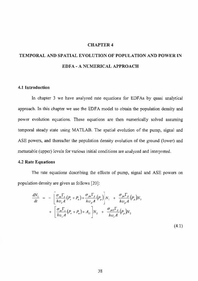
3.4 Signal and ASE Power Evolution

To understand the nature o f solutions for power obtained in the previous section,

we chose a set o f practical parameters and plotted the evolution o f signal and ASE

graphically. Fig 3.2 and Fig 3.3 show the behavior o f the ASE power and signal power

densities obtained by the numerical solutions o f the eqs. (3.1), (3.2) and (3.3) using the

parameters listed in the Table 3.1.

Table 3.1 Values o f the Parameters used to Generate Franco Plots

Ap = 514.5zizm = 1530nm

crp = 2.4 xlO -21 cm2 <ra = 4.83x10

ere = 8.1xlO~21czn2 Ps = 100/JF

r , = r , = o . 4 Pp = 50mJF

N, = 9.02x102°w -3 n2= 7.31x10

36

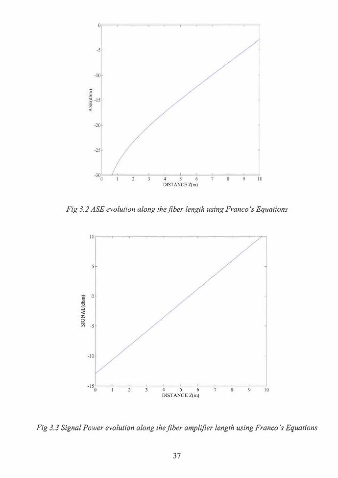
Fig 3.2 ASE evolution along the fiber length using Franco’s Equations

Fig 3.3 Signal Power evolution along the fiber amplifier length using Franco’s Equations

37

CHAPTER 4

TEMPORAL AND SPATIAL EVOLUTION OF POPULATION AND POWER IN

EDFA - A NUMERICAL APPROACH

4.1 Introduction

In chapter 3 we have analyzed rate equations for EDFAs by quasi analytical

approach. In this chapter we use the EDFA model to obtain the population density and

power evolution equations. These equations are then numerically solved assuming

temporal steady state using MATLAB. The spatial evolution o f the pump, signal and

ASE powers, and thereafter the population density evolution of the ground (lower) and

metastable (upper) levels for various initial conditions are analyzed and interpreted.

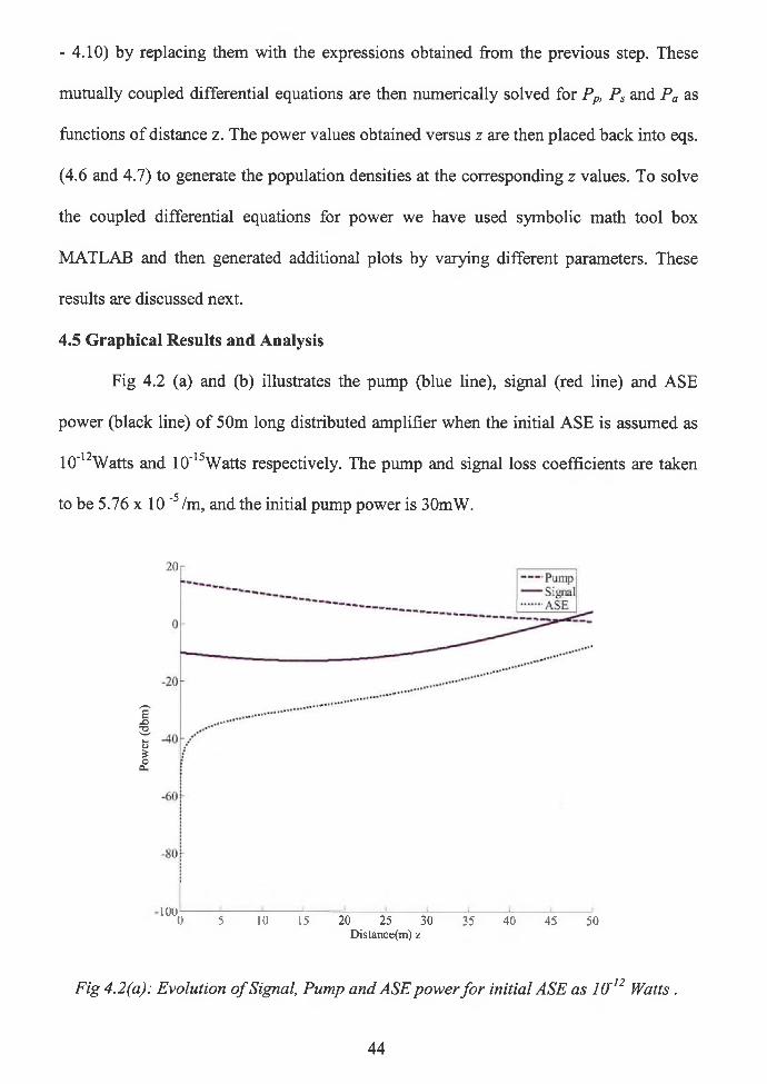
4.2 Rate Equations

The rate equations describing the effects of pump, signal and ASE powers on

population density are given as follows [20]:

dN,dt hvsA

hv.A

hopA N‘ +

(Ps +Pa)+A2i N, +hu.A

(4.1)

38

dN 2dt h v .A

(P ,+ P .)N , -T-<

+p„)+a.h o ,A [ s a/ 21

+ W ,h v pA

N ,

(4.2)

In the above equations, the absorption and emission cross sections o f the signal and

pump are os, p: a, e, e2- With pumping into the metastable level, the amplifier behaves as a

two level system and

oPe2 = Ope- Pumping into other absorption bands have ape2 = 0. Other parameters are the

fiber core area A, the signal to core overlap Ts, and the pump to core overlap Tp. The

parameters Ts and Tp are small since the erbium ions are considered to be confined to the

region of the optical mode’s peak intensity. The nonradiative transition rate from level 3

to 2 is A32 and the radiative transition rate from level 2 to 1 is A2i .

4.3. Pump Configurations

Three different pump configurations are possible for pumping a length o f erbium

doped fiber. These are: copropagating pump and signal, counter propagating pump and

signal, and bi-directional pumping, as depicted in the Fig. 4.1 (a), (b) and (c). As far as

small signal gain is concerned, copropagating and counterpropagating pumps yield the

same gain and only the total amount o f pump power matters. This is because the ASE

patterns generated by the two pump patterns are mirror images o f each other and so the

average upper state population is the same in both the cases. When the fiber is

sufficiently long, bi-directional pumping results in higher small signal gain at 1.5 pm for

equal amounts o f pump power than either the co or counter propagating pumping

patterns.

39

The copropagating pump configuration offers the lowest noise figure because the

portion o f the fiber that the signal enters tends to be more inverted than the section by

which the signal exits. Thus the signal undergoes more gain per unit length at the

beginning of the fiber than at the exit. In the counter propagating configuration, lower

gain per unit length at the beginning o f the fiber is equivalent to having some amount of

loss for the signal before it enters the amplifier. Any loss that the signal experiences at

the beginning of the fiber will degrade the noise figure. Thus, in the absence o f any other

effects, the copropagating pump configuration is preferred for obtaining a low noise

figure.

Er-doped fiber

Fig 4.1 (a): Copropagating Pump and Signal [24],

Signal out

Fig 4.1 (b): Counter Propagating Pump and Signal [24],

Signal out

40

Er-doped fiber

4.4 Solution for the EDFA Rate Equations - Numerical Representation

In steady state, we assume Nj and N2 to be independent o f time. This can be justified

since the settling period o f the population densities is in the order o f 10'5 - IO-6 sec [49].

Thus,

dN,dt

0 , and

(4.3)

(4.4)

Consider also

N 3 = N t - N , - N 2,

(4.5)

Where Nt is the total population o f particles (erbium ions). By grouping the coefficients

for the population densities individually yields eq. (4.6) and eq. (4.7) from eqs. (4.1 and

4.2) respectively.

41

The propagation equations [20] for the pump, signal and ASE field powers are given as:

(4.8)

- « Z » a n d

(4.9)

+ 2a„N2TshDsLo - asPa.

(4.10)

The ojr and oj, represent the internal loss terms. The second term in eq. (4.10) gives

the ASE power produced in an amplifier per unit length. The power produced is within

the amplifier bandwidth An, which is homogeneously broadened. The internal loss o f the

amplifier usually corresponds to signal and pump attenuation in the transmission fiber.

The values o f all the parameters used in the eqs. (4.6 - 4.10) are given in Table 4.1 [20].

Table 4.1 Fiber Amplifier Parameters used in Calculations

a p =1480 nm z s =1545 nm

<rpe = 0.42 x 10~21 cm2 cr = 1.86x 10~21ctm2

<rse = 5.03 x IO-21 cw2 <7 = 2 .8 5 x 10’21cw2sa

>f21 =100s_1 A32 = 109s ~1

A = 12.6x 10~8cw2 At? = 3100 GHz(25 nm)

r = r = 0.4

The signal chosen for amplification is o f the wavelength 1550 nm approximately,

and a 1480 nm pump is used instead of 980 nm. This is because the 1480 nm pump

provides a higher gain than the 980 nm pump [24]. The 1480 nm pump can maintain the

necessary inversion levels over significantly longer lengths than the 980 nm pump. The

reason for this is the higher quantum efficiency o f 1480 nm pumping. This allows the

signal to grow to a higher maximum value.

4.4.1 Numerical Approach

For the numerical approach, the rate o f change o f population levels with respect to

time is neglected, thereby assuming steady state. However, the population levels are

assumed to be varying with distance z. From eqs. (4.1 and (4.2), Ni and N2 are solved in

terms o f the pump, signal and ASE powers. Next, Ni and N2 are eliminated from eqs. (4.8

43

- 4.10) by replacing them with the expressions obtained from the previous step. These

mutually coupled differential equations are then numerically solved for Pp, Ps and Pa as

functions o f distance z. The power values obtained versus z are then placed back into eqs.

(4.6 and 4.7) to generate the population densities at the corresponding z values. To solve

the coupled differential equations for power we have used symbolic math tool box

MATLAB and then generated additional plots by varying different parameters. These

results are discussed next.

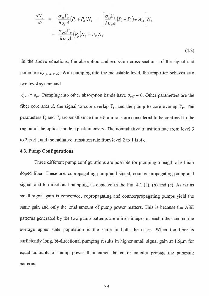
4.5 Graphical Results and Analysis

Fig 4.2 (a) and (b) illustrates the pump (blue line), signal (red line) and ASE

power (black line) o f 50m long distributed amplifier when the initial ASE is assumed as

10’12Watts and 10’15Watts respectively. The pump and signal loss coefficients are taken

to be 5.76 x 10 '5 /m, and the initial pump power is 30mW.

ioo---------- ----------------------------------0 5 10 15 20 25 30 35 40 45 50

Distance(m) z

Fig 4.2(a): Evolution o f Signal, Pump and ASE power fo r initial ASE as IO'12 Watts .

44

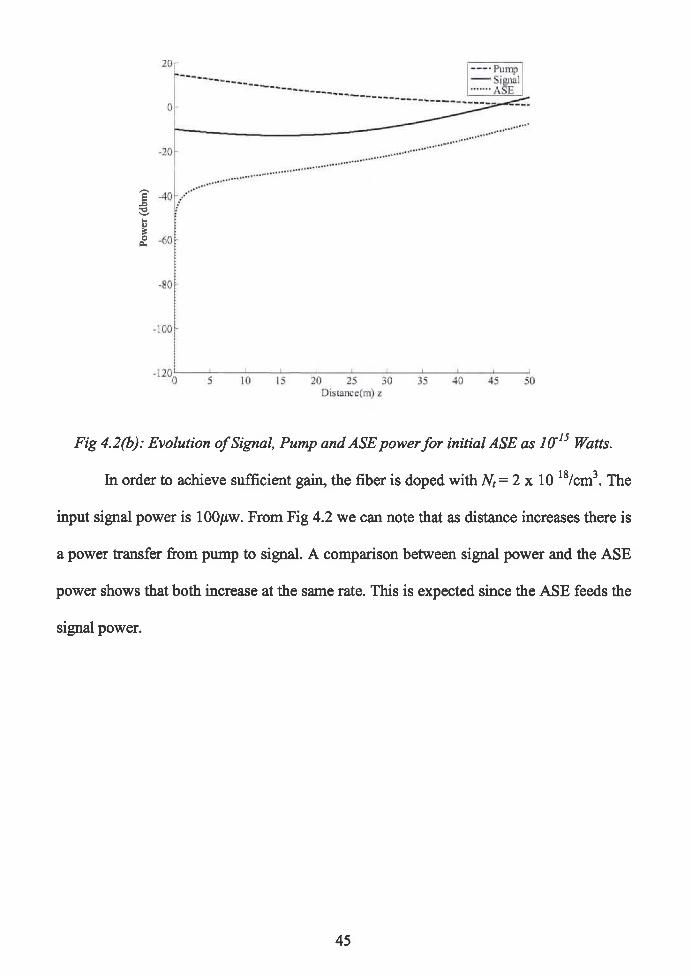
Fig 4.2(b): Evolution o f Signal, Pump and ASE power fo r initial ASE as I f f 15 Watts.

In order to achieve sufficient gain, the fiber is doped with Nt = 2 x 10 18/cm3. The

input signal power is 100/xw. From Fig 4.2 we can note that as distance increases there is

a power transfer from pump to signal. A comparison between signal power and the ASE

power shows that both increase at the same rate. This is expected since the ASE feeds the

signal power.

45

4.5.1 Population Inversion

Fig 4.3: Population Evolution o f Ground level (Nj) and Metastable level (N2) in EDFA

Fig 4.3 (a): Gain Plot fo r EDFA

46

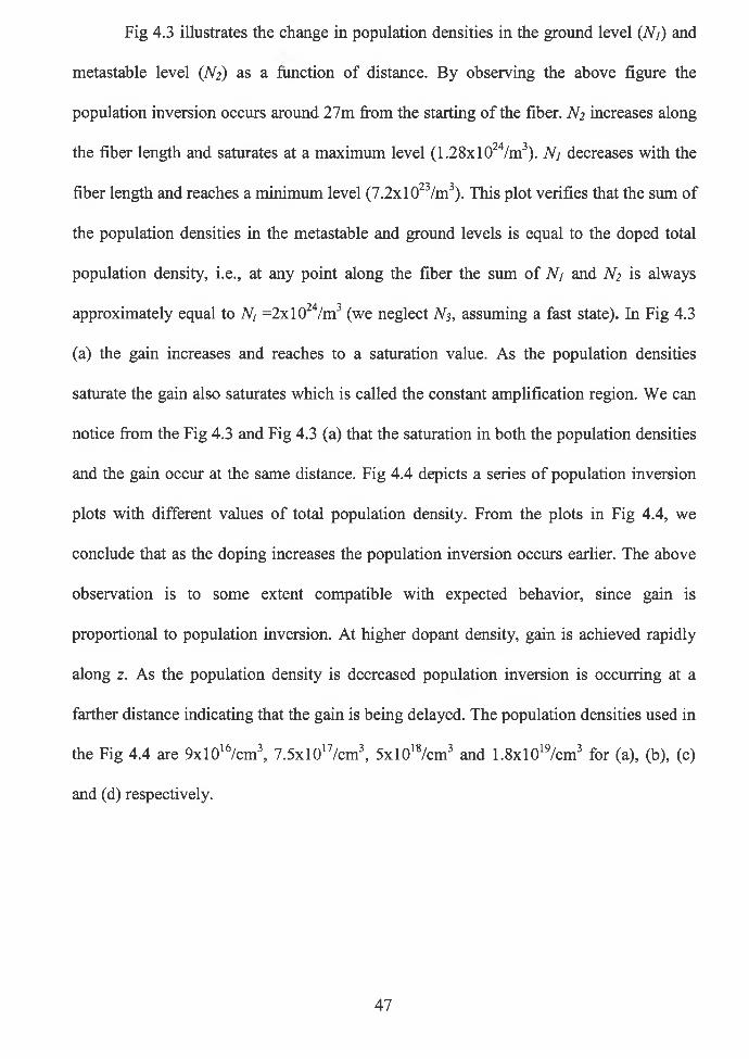
Fig 4.3 illustrates the change in population densities in the ground level (TV;) and

metastable level (TVj) as a function of distance. By observing the above figure the

population inversion occurs around 27m from the starting o f the fiber. N2 increases along

the fiber length and saturates at a maximum level (1.28xl024/m3). TV; decreases with the

fiber length and reaches a minimum level (7.2x1023/m3). This plot verifies that the sum of

the population densities in the metastable and ground levels is equal to the doped total

population density, i.e., at any point along the fiber the sum o f TV; and TV2 is always

approximately equal to TV, =2xl024/m3 (we neglect TV;, assuming a fast state). In Fig 4.3

(a) the gain increases and reaches to a saturation value. As the population densities

saturate the gain also saturates which is called the constant amplification region. We can

notice from the Fig 4.3 and Fig 4.3 (a) that the saturation in both the population densities

and the gain occur at the same distance. Fig 4.4 depicts a series o f population inversion

plots with different values o f total population density. From the plots in Fig 4.4, we

conclude that as the doping increases the population inversion occurs earlier. The above

observation is to some extent compatible with expected behavior, since gain is

proportional to population inversion. At higher dopant density, gain is achieved rapidly

along z. As the population density is decreased population inversion is occurring at a

farther distance indicating that the gain is being delayed. The population densities used in

the Fig 4.4 are 9 x l0 16/cm3, 7 .5xl017/cm3, 5x l018/cm3 and 1.8xl019/cm3 for (a), (b), (c)

and (d) respectively.

47

(a)

DuUnccim)

(c)

(b)

Dwtanee(n])

(d)

Fig 4.4: Population Inversion fo r Different Population Densities.

48

4.5.2 Variation of Input Signal Power

-40; — ■ ------ ----------- — ' - - — ----- 10 10 20 30 40 50 60 70 80 90 100

Distance(m) z

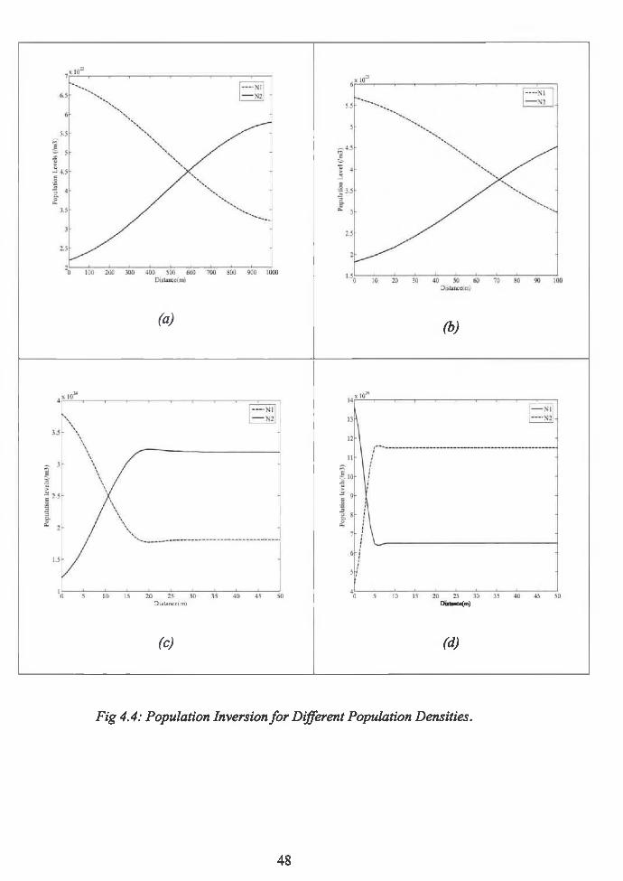
Fig 4.5: Variation o f Output Signal Power fo r Different Input Signal Powers

For a particular length o f amplification section the gain is constant. So, as the

input signal power is increased the output signal power must increase in order to keep the

gain constant. Fig 4.5 shows that signal variation with different input signal powers for a

IO opopulation density Nt = 2x10 /cm , initial pump power o f 30mW, pump wavelength

= 1480nzn and signal wavelength = 1545hwj .

From Fig 4.7 we can note that for higher input signal powers the decay in the

pump power is less. This is also evident from eq. 4.8 which is a pump power variation

along the propagation distance, depends upon the input signal power.

49

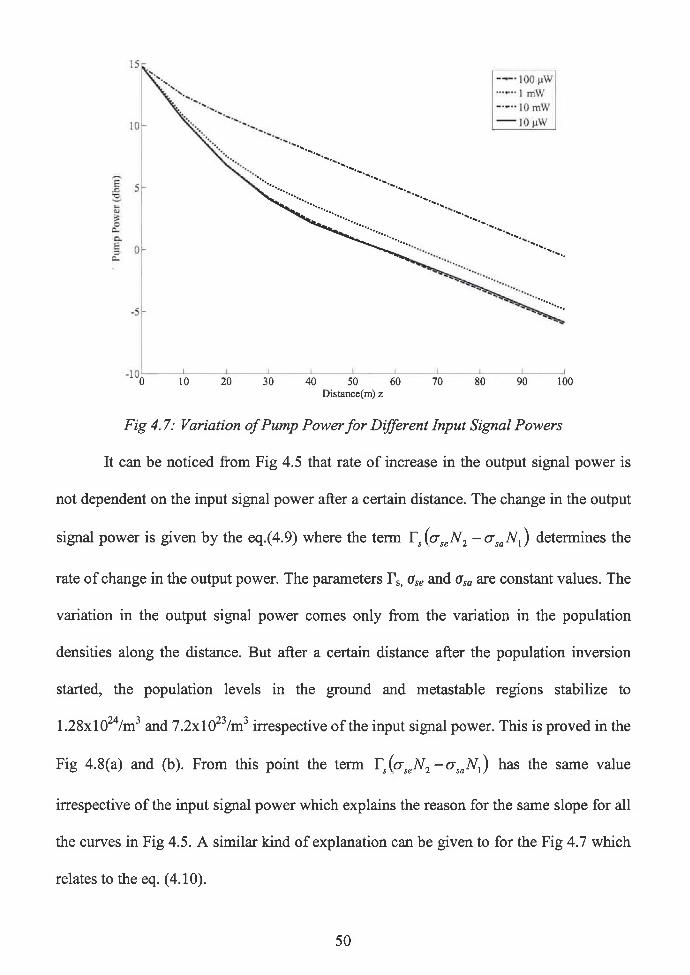
Fig 4.7: Variation o f Pump Power fo r Different Input Signal Powers

It can be noticed from Fig 4.5 that rate o f increase in the output signal power is

not dependent on the input signal power after a certain distance. The change in the output

signal power is given by the eq.(4.9) where the term Ys(<jseN 2 -<TsaA ,) determines the

rate o f change in the output power. The parameters Ts> ose and oSa are constant values. The

variation in the output signal power comes only from the variation in the population

densities along the distance. But after a certain distance after the population inversion

started, the population levels in the ground and metastable regions stabilize to

1.28xl024/m3 and 7.2xl023/m3 irrespective o f the input signal power. This is proved in the

Fig 4.8(a) and (b). From this point the term Ys(aseN 2 - a saN ^ has the same value

irrespective o f the input signal power which explains the reason for the same slope for all

the curves in Fig 4.5. A similar kind o f explanation can be given to for the Fig 4.7 which

relates to the eq. (4.10).

50

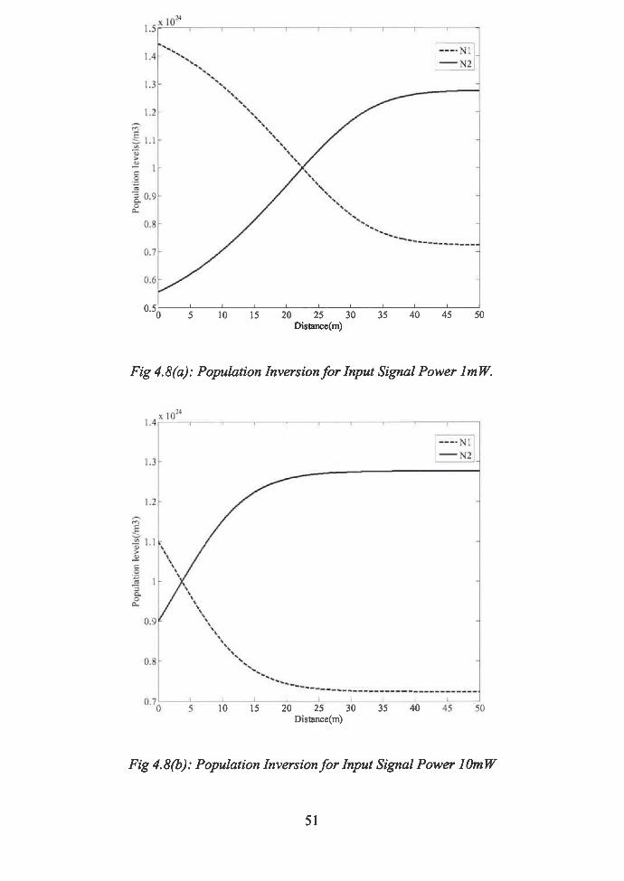
Fig 4.8(a): Population Inversion fo r Input Signal Power I mW.

Fig 4.8(b): Population Inversion fo r Input Signal Power lOmW

51

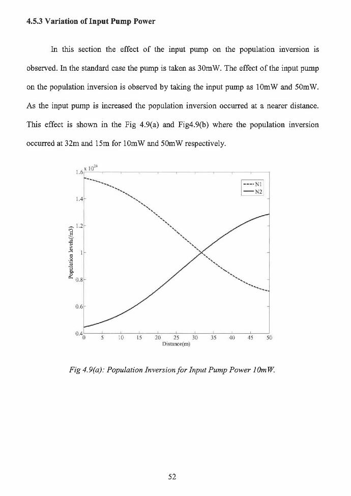
4.5.3 Variation of Input Pump Power

In this section the effect o f the input pump on the population inversion is

observed. In the standard case the pump is taken as 30mW. The effect o f the input pump

on the population inversion is observed by taking the input pump as lOmW and 50mW.

As the input pump is increased the population inversion occurred at a nearer distance.

This effect is shown in the Fig 4.9(a) and Fig4.9(b) where the population inversion

occurred at 32m and 15m for lOmW and 50mW respectively.

Fig 4.9(a): Population Inversion fo r Input Pump Power 10m W.

52

Fig 4.9(b): Population Inversion fo r Input Pump Power 50mW.

4.5.4 Variation of Pump and Signal Wavelength

Distance(m) z

Fig 4.10(a): Variation o f Output Signal Power fo r Different Pump Wavelengths

53

15-

Fig 4.10(b): Variation o f Pump Power fo r Different Pump Wavelengths

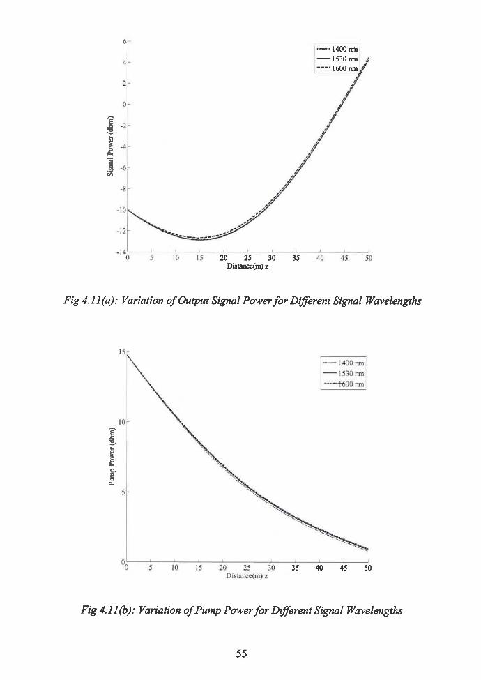
Fig 4.10(a) and (b) show the variation o f signal and pump power for different

pump wavelengths for a population density Nt = 2 x l0 18/cm3, signal wavelength

A, = 1545nm , initial pump power o f 30mW and input signal power o f lOOpW. Higher the

wavelength (lower frequency) energy in the pump is less. This leads to the following

result. As the pump wavelength increases the amplification o f the signal is less and the

decay in the pump power is more. The same thing happens with the variation in signal

wavelength. This is shown in Fig 4.11(a) and (b).

54

6

Fig 4.11(a): Variation o f Output Signal Power fo r Different Signal Wavelengths

Fig 4.11(b): Variation ofPump Power fo r Different Signal Wavelengths

55

4.5.4.1 Effect o f Pump and Signal Wavelength on Population Inversion

Variation o f the pump wavelength did not shift the position o f the population

inversion proportionately in the amplifier. This is shown in the series o f the plots as Fig

4.12(a), (b), (c) where the pump wavelength is assumed as 1480nm, 1510nm, 1550nm.

Fig 4.12(a): Population Inversion fo r Pump Wavelength 1480nm.

56

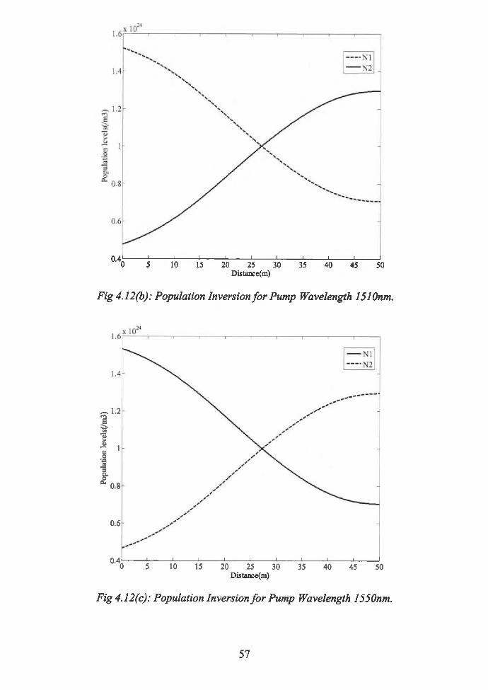
Fig 4.12(b): Population Inversion fo r Pump Wavelength 1510nm.

Fig 4.12(c): Population Inversion fo r Pump Wavelength 1550nm.

57

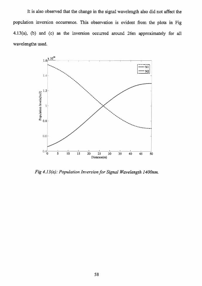
It is also observed that the change in the signal wavelength also did not affect the

population inversion occurrence. This observation is evident from the plots in Fig

4.13(a), (b) and (c) as the inversion occurred around 26m approximately for all

wavelengths used.

Fig 4.13(a): Population Inversion fo r Signal Wavelength 1400nm.

58

Fig 4.13(b): Population Inversion fo r Signal Wavelength 1530nm.

Fig 4.13(c): Population Inversion fo r Signal Wavelength 1600nm.

59

4.6 Optimum Parameter Values

The parameters that we could vary during the computations were the input pump

power, input signal power, pump wavelength, signal wavelength and the initial

population density o f the erbium doping. Our goal is to achieve the population inversion

in the least distance possible. For this, we have varied all the above mentioned parameters

and noticed that enhanced energy transfer effectively results from the variation o f the

input pump power and the erbium doping as compared to the variation of signal and

pump wavelengths in the previous sections. The increase in the input signal strength also

shifted the point of population inversion to a closer point. This is explicit as the increase

in signal strength would increase the gain and hence the variation in this parameter is not

considered for optimization. As the pump power increased the population inversion

occurred at a closer point. The same effect is seen for the variation o f the erbium doping

which is the total population density. So keeping all the other parameter values at the

regular values as shown in the Table 4.1 we have varied the pump power and the

population density. We have considered the population density N t = 5 x 1018 and the input

pump power as 50mW for one case. At these values the population inversion occurred at

around 6.1m as shown in Fig 4.14. In the second case we have further increased the

erbium doping to N, = 8 x l0 18 keeping the pump power at 50mW. Under these

conditions the population inversion moved much closer and occurred at around 3.8m as

shown in Fig 4.15.

60

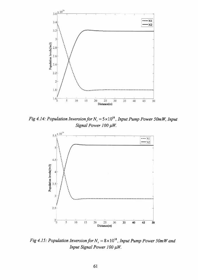
Fig 4.14: Population Inversion fo r N t = 5xl018, Input Pump Power 50mW, Input Signal Power 100 pW.

Fig 4.15: Population Inversion fo rN , = 8 x 1018, Input Pump Power 50m W and Input Signal Power 100 pW.

61

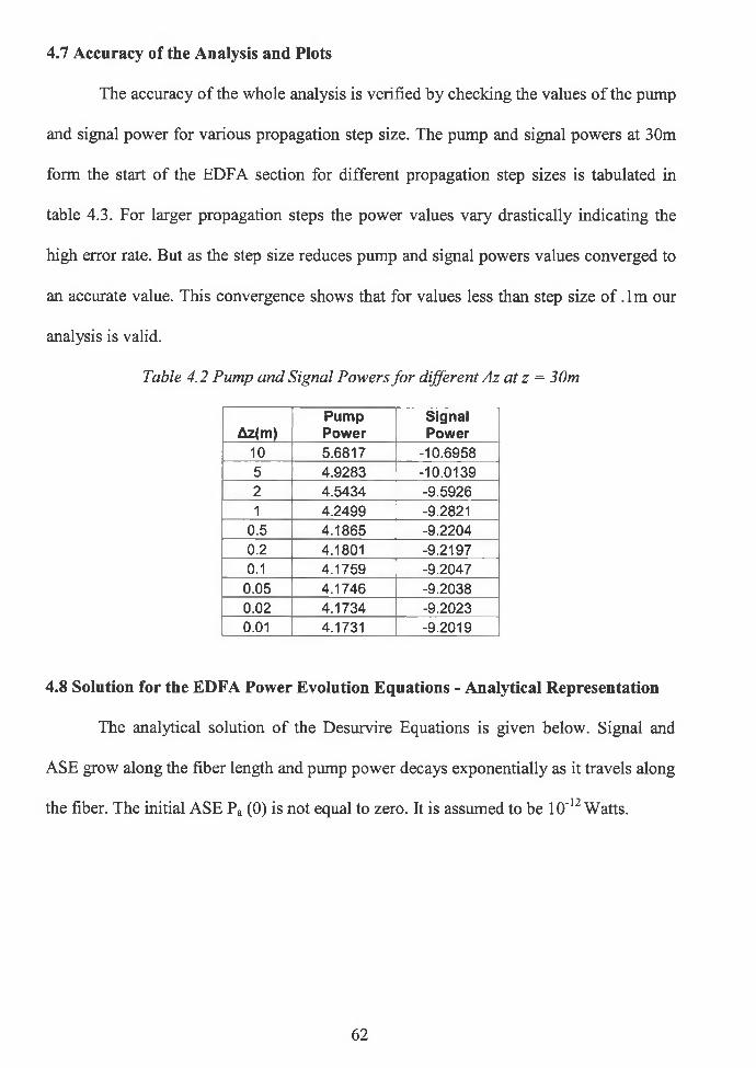
4.7 Accuracy of the Analysis and Plots

The accuracy of the whole analysis is verified by checking the values o f the pump

and signal power for various propagation step size. The pump and signal powers at 30m

form the start o f the EDFA section for different propagation step sizes is tabulated in

table 4.3. For larger propagation steps the power values vary drastically indicating the

high error rate. But as the step size reduces pump and signal powers values converged to

an accurate value. This convergence shows that for values less than step size o f .lm our

analysis is valid.

Table 4.2 Pump and Signal Powers fo r different Az at z = 30m

Az(m)PumpPower

SignalPower

10 5.6817 -10.69585 4.9283 -10.01392 4.5434 -9.59261 4.2499 -9.2821

0.5 4.1865 -9.22040.2 4.1801 -9.21970.1 4.1759 -9.2047

0.05 4.1746 -9.20380.02 4.1734 -9.20230.01 4.1731 -9.2019

4.8 Solution for the EDFA Power Evolution Equations - Analytical Representation

The analytical solution o f the Desurvire Equations is given below. Signal and

ASE grow along the fiber length and pump power decays exponentially as it travels along

the fiber. The initial ASE Pa (0) is not equal to zero. It is assumed to be 10'12 Watts.

62

PP(z) = Pp(Q) exp(-;4iz)Ps(z) = Ps(O) exp(^2z)P ,(z) = e\p(A-,(z + hl( ^ 4 /^ ) ) )

A3A\ — [(OpoTV 1 — OpeN2)!""p + GpJ A2 = A3 = [((JseN2 ~ OsaNi)D - Cfc]

At, = 2aseN 2h UsY sA u

4.8 Conclusion

Franco neglected attenuation in the transmission fiber. Moreover, Franco’s

equations are power spectral density equations and Desurvire’s equations are power

equations. The detailed analysis in this chapter shows that, in the case o f pure numerical

solutions, the ASE and signal power increase along the length o f the EDFA section. But

taking a closer look on the signal power more realistic pump power fitting will lead to

accurate signal power evolution. The set o f eqs. (3.1), (3.2) and (3.3) when compared

with the (4.8), (4.9) and (4.10) eqs. respectively look structurally symmetric.

63

CHAPTER 5

SUMMARY AND CONCLUSIONS

5.1 Summary:

To overcome the problem o f signal attenuation during long distance propogation,

electronic regenerators limited by the speed o f the electronic components have been used

for many years. With the advent o f fiber optic communications, electronic regenerators

are being replaced by optical amplifiers based on the phenomenon o f stimulated

emission. Optical amplifiers serve fiber communication systems in several ways. Since

the 80s, many researchers and scientists throughout the world have worked to improve

amplifiers so as to increase their bandwidth and channel capacity.

SLAs, Raman amplifiers, Brillouin amplifiers and rare earth ion doped fiber

amplifiers are different types o f fiber amplifiers that have been used for amplification

purposes [23]. Certain characteristics such as gain saturation, ASE power, noise figure

and signal gain define an optical amplifier. In-line amplifiers, power amplifiers, LAN

amplifiers are some examples o f the applications o f optical amplifiers. O f the different

kinds of optical amplifiers we have analyzed the erbium doped fiber amplifiers (EDFAs)

because they have better cross-talk characteristics, higher operating power, lower

insertion loss, broader bandwidth, higher efficiency and low noise figure. In addition,

64

they can be used both as distributed and lumped amplifiers. The architecture,

characteristics and the spectrum of erbium dopant are also discussed.

The three level laser system model [24] for the evolution o f signal and ASE

power due to an applied pump power is found to be an easy and efficient way of

analyzing the EDFA section in fiber communications. We have analyzed the evolution

equations for signal and ASE power densities using the numerical method given in

chapter 4. This method is found to be so much at bit tedious, but accurate. The growth of

the population densities o f both ground and metastable levels is numerically solved under

temporal steady state in the direction of propagation. The resulting population densities

illustrate the occurrence o f population inversion at a cross over point which leads to the

amplification in EDFAs. The evolution equations which are solved numerically, are also

plotted by varying parameters such as initial pump and input signal powers, the level of

erbium doping, and pump and signal wavelengths within the optimum range. The effects

o f these parameters on the behavior o f the EDFA have been analyzed. Based on these

results, an optimum set o f values has been suggested for the parameters in order to obtain

the population inversion in the shortest possible distance (approximately less than 10m).

Further we used quasi analytical solution fitting for the rate equations as suggested by P.

Franco [22] and a more exact result solved from a modified set o f equations. The trends

in the plots generated using the solution appear to match with the numerical solution

suggested by E. Desurvire [20],

5.2 Future Work:

We have solved the spatial evolution equation for the EDFA section for temporal

steady state conditions. If we consider non steady state in both space and time we obtain

65

highly nonlinear coupled differential equations; ideally, solutions to such equations

would provide better insight into the transient dynamics o f population and power. This

may be pursued as an extension o f this work. Moreover, in the quasi analytical solution

for the rate equation suggested in chapter 3 consist o f only few parameters. We can add

more parameters such as the attenuation losses o f signal and power in the fiber to the

power equation solution fitting, which will yield a precise result. Before making a fitting

we should compare and analyze the solution between the two methods suggested in

chapters 3 and 4. This will allow us to choose an optimum set o f parameters, so that the

computation does not become large, and the result obtained is precise with in an error

margin.

66

Bibliography

1. J. E. Geusic and H. E. D. Scovil, “A unidirectional traveling-wave optical laser,” Bell Syst. Tech. J. 41, 1371 (1962).

2. E. Snitzer and R. Woodcock, “Yb3+-Er3+ glass laser,” Appl. Phys. Lett. 6, 45 (1965).

3. J. Stone and C. A. Burrus, “Neodymium-doped silica lasers in end-pumped fiber geometry,” Appl. Phys. Lett. 23, 388 (1973).

4. R. J. Mears, L. Reekie, I. M. Jaunice, and D. N. Payne, “High-gain rare-earth doped fiber amplifier at 1.54 pm,” Optical Fiber Communication Conference. 3, 167(1987)

5. E. Snitzer, H. Po, F. Hakimi, R. Tuminelli, and B. C. MaCollum, “Erbium fiber laser amplifier at 1.55 pm with pump at 1.49 pm and Yb sensitized Er oscillator,” Optical Fiber Communication Conference. 1, 218 (1988).

6. M. Nakazawa, K. Suzuki, and Y. Kimura, “Efficient Er3 + - doped optical fiber amplifier pumped by a 1.48 pm InGaAsP laser diode,” Appl. Phys. Lett. 54, 295 (1989).

7. N. A. Olsson, J. Light. Tech. 7, 1071 (1989).

8. N. Edagawa, K. Mochizuki, and H. Wakabayashi, “ 1.2Gbit/s, 218 km Transmission Experiment Using Inline Er-Doped Fibre Amplifier,” Elect. Lett. 25, 363 (1989).

9. S. B. Poole, D. N. Payne, and M. E. Fermann, “Fabrication of low loss optical fibers containing rare-earth ions,” Elect. Lett. 21, 737 (1985).

10. L. Reekie, R. J. Mears, S. B. Poole and D. N. Payne, “Tunable single-mode fiber lasers,” J. Light. Tech. 4, 956 (1986).

11. R. J. Mears et.al., “High-gain rare-earth doped fiber amplifier at 1.54 pm,” Optical Fiber Communication Conference. 12, 19 (1987).

67

12. C. A. Millar, “Thermal properties o f an erbium-doped fiber amplifier,” Elect. Lett. 23, 865 (1987).

13. L. Reekie, I. M. Jauncey, S. B. Poole, and D. N. Payne, “Diode Laser pumped operation of an Er3+ doped single mode fiber laser,” Elect. Lett. 23, 1076 (1987).

14. R. I. Laming, S. B. Poole, and E. J. Tarbox, “Pump excited-state absorption in erbium-doped fibers,” Opt. Lett. 13, 1084 (1988).

15. E. Desurvire et.al., “2-Gbit/s signal amplification at X=1.53 /xm in an erbium- doped single-mode fiber amplifier,” Opt. Lett. 14, 1266 (1989).

16. Y. Kimura, K. Suzuki, and M. Nakazawa, “Soliton amplification and transmission with Er3+-dopedfibre repeater pumped by GalnAsP diode,” Elect. Lett. 25, 1656 (1989).

17. E. Desurvire, C. R. Giles, and J. R. Simpson, “Saturation-induced crosstalk in high speed erbium doped fiber amplifiers at I = 1.53 /xm,” Optical Fiber Communication Conference. 7, 14 (1989).

18. R. E. Wagner et.al., “ 16-channel coherent broadcast network at 155 Mb/s,” Optical Fiber Communication Conference. 12, 21 (1989).

19. H. Taga et.al., “459 km, 2.4 Gbit/s 4 wavelength multiplexing optical fiber transmission experiment using 6 Er-doped fiber amplifiers,” Optical Fiber Communication Conference. 9, 23 (1990).

20. C. R. Giles and E. Desurvire, “Propagation of Signal and Noise in Concatenated Erbium Doped Fiber Optical Amplifiers,” J. Light. Tech 9, 147 (1991).

21. E. Desurvire and J. R. Simpson, “Amplification o f Spontaneous Emission in Erbium-Doped Single-Mode Fibers,” J. Light. Tech. 7, 835 (1989).

22. Pierluigi Franco and Michele Midrio, “Quasi-analytic solution o f erbium-doped fiber-amplifier power equations,” Appl. Opt. 32, 7442 (1993).

23. G. P. Agrawal, Fiber- Optic Communication Systems. New York: John Wiley & Sons, 1992.

24. P. C. Becker, N. A. Olsson and J. R. Simpson, Erbium Doped Fiber Amplifiers: Fundamentals and Technology. San Diego: Academic Press, 1999.

25. J. Hecht, “The Evolution of Optical Amplifiers,” Optical and Photonics News 13, 36 (2002).

68

26. Hansel E. Lee Jr., “A research paper on Erbium Doped fiber Amplifiers,” Optical Comm. Systems, (1996). Available at http://hansel.hansel.com/papers/erbium.html

27. E. Desurvire, Erbium Doped Fiber Amplifiers: Principles and Applications. New York: John Wiley & Sons, 1987

28. E. Desurvire, J. R. Simpson, and P. C. Becker, “High-gain erbium-doped traveling-wave fiber amplifier,” Opt. Lett. 12, 888 (1987).

29. K. Nakagawa, S. Nishi, K. Aida, and E. Yoneda, “Trunk and distribution network application of erbium-doped fiber amplifier,” J. Light. Tech. 9, 198 (1991)

30. Mukai, T., K. Inoue and T. Saito, “Homogeneous gain saturation in 1.5mm InGaAsP traveling wave semiconductor laser amplifiers,” Appl. Phys. Lett. 51, 366 (1987).

31. M. J. F. Digonnet, Rare Earth Doped Fiber Lasers and Amplifiers. New York: Marcel Dekker Inc, 1993.

32. R. H. Stolen, E. P. Ippen, and A.R. Tynes, “Raman oscillation in glass Optical waveguides,” Appl. Phys. Lett. 20, 62 (1972);R. H. Stolen and E. P. Ippen, “Raman gain in glass optical waveguides,” Appl. Phys. Lett. 22, 276 (1973).

33. N. Edagawa, K. Mochizuki, S. Ryu and H. Wakabayashi, “Amplification characteristics o f fiber Raman Amplifiers,” ICICE Technical Report. 88, 33 (1988).

34. C. G. Atkins, D. Cotter, D.W. Smith and R. Wyatt, “Application o f Brillouin amplification in coherent optical transmission,” Elect. Lett. 22, 348 (1986).

35. R. J. Mears, L. Reekie, I. M. Jauncey, and D. N. Payne, “Low-Noise Erbium- Doped Fiber Amplifier Operating at 1.54pm,” Elect. Lett. 23, 1026 (1987).

36. B. E. A. Saleh and M. C. Teich, Fundamentals o f Photonics, New York: John Wiley & Sons, 1991.

37. C. Bendjaballah and M. Charbit, “Detection of optical signals in generalized Gaussian noise,” IEEE Trans. Comm. 73, 1840 (1983).

38. M. J. F. Digonnet, “Closed-form expressions for the gain in three- and four-level laser fibers,” IEEE J. Quant. Elect. 26, 1788 (1990).

39. Y. Ohishi, T. Kanamori, T. Kitagawa, S. Takahashi, E. Snitzer and G. H. Sigel, “Pr3+ doped fluoride fiber amplifier operating at 1.31pm,” Optical Fiber Communication Conference. 4, 237 (1991).

69

40. M. Shimizu, T. Kanamori, J. Temmyo, M. Wada, M. Yamada, Y. Terunuma, Y. Ohishi and S. Sudo, “28.3 dB gain 1.3gm band Pr-doped fluoride fiber amplifier module pumped by 1.017/im InGaAs - LD’s,” IEEE Phot. Tech. Lett. 5, 654 (1993).

41. M. Yamada, M. Shimizu, T. Kanamori, Y. Ohishi, Y. Terunuma, K. Oikawa, H. Yoshinaga, K. Kikushima, Y. Miyamoto, and S. Sudo, “Low-noise and high - power Pr3+ -doped fluoride fiber amplifier,” IEEE Phot. Tech. Lett. 7, 869 (1995).

42. S. Sanders, K. Dzurko, R. Parke, S. O’Brien, D. F. Welch, S. G. Grubb, G. Nykolak, and P. C. Becker, “Praseodymium doped fibre amplifiers (PDFAs) pumped by monolithic master oscillator power amplifier (M-MOPA) laser diodes,” Elect. Lett. 32, 343 (1993).

43. M. L. Dakss and W. J. Miniscalco, “A large-signal model and signal/noise ratio analysis for Nd3+ doped fiber amplifiers at 1.3/xm,” Fiber Laser Sources and Amplifiers II. 1373, 111 (1990).

44. W. J. Miniscalco, L. J. Andrews, B. A. Thompson, R. S. Quimbly, L. J. B. Vacha, and M. G. Drexhage, “1.3 pm fluoride fibre laser,” Elect. Lett. 24, 28 (1988).

45. M. Brierley, S. Carter, P. France, and J. E. Pederson, “Amplification in the 1300 nm telecommunications window in an Nd-doped fluoride fiber,” Elect. Lett. 26, 330 (1990).

46. Y. Miyajima, T. Sugawa, and T. Komukai, “ 10 dB gain and high saturation in a Nd3+ - doped fluorozirconate fiber amplifier,” Elect. Lett. 26, 1398 (1990).

47. E. Ishikawa, H. Aoki, T. Yamashita, and Y. Asahara, “Laser emission and amplification at 1.3gm in neodymium - doped fluorophosphates fibres,” Elect. Lett. 28, 1497 (1992).

48. Vivek Mehta., Amplified Spontaneous Emission available at http ://light.utoronto .ca/vmehta/ase.pdf

70