Numerical block diagonalization of matrix

∗-algebras with application to semidefinite

programming

Etienne de Klerk∗ Cristian Dobre† Dmitrii V. Pasechnik‡

November 21, 2009

Abstract

Semidefinite programming (SDP) is one of the most active areas inmathematical programming, due to varied applications and the availabil-ity of interior point algorithms. In this paper we propose a new pre-processing technique for SDP instances that exhibit algebraic symmetry.We present computational results to show that the solution times of cer-tain SDP instances may be greatly reduced via the new approach.

Keywords: semidefinite programming, algebraic symmetry, pre-processing, in-terior point methods

AMS classification: 90C22∗Department of Econometrics and OR, Tilburg University, The Netherlands.

e.deklerk@uvt.nl†Department of Econometrics and OR, Tilburg University, The Netherlands.

c.dobre@uvt.nl‡Division of Mathematical Sciences, SPMS, Nanyang Technological University, 21 Nanyang

Link, 637371 Singapore. dima@ntu.edu.sg

1

1 Introduction

Semidefinite programming (SDP) is currently one of the most active areas ofresearch in mathematical programming. The reason for this is two-fold: appli-cations of SDP may be found in control theory, combinatorics, real algebraicgeometry, global optimization and structural design, to name only a few; see thesurveys by Vandenberghe and Boyd [29] and Todd [26] for more information.The second reason is the extension of interior point methods from linear pro-gramming (LP) to SDP in the 1990’s by Nesterov and Nemirovski [22], Alizadeh[1], and others.

A recurrent difficulty in applying interior point methods for SDP is that itis more difficult to exploit special structure in the data than in the LP case. Inparticular, sparsity may readily be exploited by interior point methods in LP,but this is not true for SDP. Some structures in SDP data have been exploitedsuccessfully, see the recent survey [11] for details.

Of particular interest for this paper is a structure called algebraic symme-try, where the SDP data matrices are contained in a low-dimensional matrixC∗-algebra. (Recall that a matrix ∗-algebra is a linear subspace of Cn×n thatis closed under multiplication and taking complex conjugate transposes.) Al-though this structure may seem exotic, it arises in a surprising number of ap-plications, and first appeared in a paper by Schrijver [23] in 1979 on boundsfor binary code sizes. (Another early work on algebraic symmetry in SDP is byKojima et al. [16].)

More recent applications are surveyed in [11, 7, 28] and include bounds onkissing numbers [2], bounds on crossing numbers in graphs [12, 13], boundson code sizes [24, 9, 17], truss topology design [10, 3], quadratic assignmentproblems [14], etc.

Algebraic symmetry may be exploited since matrix C∗-algebras have a canon-ical block diagonal structure after a suitable unitary transform. Block diagonalstructure may in turn be exploited by interior point algorithms.

For some examples of SDP instances with algebraic symmetry, the requiredunitary transform is known beforehand, e.g. as in [24]. For other examples, likethe instances in [12, 13], it is not.

In cases like the latter, one may perform numerical pre-processing in orderto obtain the required unitary transformation. A suitable algorithm is given in[5], but the focus there is on complexity and symbolic computation, as opposedto practical floating point computation. Murota et al. [21] presented a practicalrandomized algorithm that may be used for pre-processing of SDP instanceswith algebraic symmetry; this work has recently been extended by Maeharaand Murota [19].

In this paper, we propose another numerical pre-processing approach in thespirit of the work by Murota et al. [21], although the details are somewhat dif-ferent. We demonstrate that the new approach may offer numerical advantagesfor certain group symmetric SDP instances, in particular for the SDP instancesfrom [13]. In particular, we show how to solve one specific instance from [13] in afew minutes on a PC after pre-processing, where the original solution (reported

2

in [13]) required a week on a supercomputer.

Outline

This paper is structured as follows. After a summary of notation we review thebasic properties of matrix C∗-algebras in Section 2. In particular, the canon-ical block decomposition is described there, and two conceptual algorithms tocompute it in two steps are given in Sections 3 and 4.

In this paper we will apply these algorithms not to the given matrix C∗-algebra, but to its so-called regular ∗-representation, described in Section 5.

In Section 6 we review how these algorithms may be used to reduce the sizeof SDP instances with algebraic symmetry, and we summarize the numericalalgorithm that we propose in this paper.

We relate our approach to the earlier work of Murota et al. [21] in Section7, and conclude with Section 8 on numerical experiments.

Notation and preliminaries

The space of p× q real (resp. complex) matrices will be denoted by Rp×q (resp.Cp×q), and the space of k × k symmetric matrices by Sk×k.

We use In to denote the identity matrix of order n. Similarly, Jn denotesthe n× n all-ones matrix. We will omit the subscript if the order is clear fromthe context.

A complex matrix A ∈ Cn×n may be decomposed as

A = Re(A) +√−1Im(A),

where Re(A) ∈ Rn×n and Im(A) ∈ Rn×n are the real and imaginary parts of A,respectively. The complex conjugate transpose is defined as:

A∗ = Re(A)T −√−1Im(A)T ,

where the superscript T denotes the transpose.A matrix A ∈ Cn×n is called Hermitian if A∗ = A, i.e. if Re(A) is symmetric

and Im(A) is skew-symmetric. If A is Hermitian, then A � 0 means A is positivesemidefinite. A matrix Q ∈ Cn×n is called unitary if Q∗Q = I. A real unitarymatrix is called orthogonal.

2 Basic properties of matrix *-algebras

In what follows we give a review of decompositions of matrix ∗-algebras overC, with an emphasis on the constructive (algorithmic) aspects. Our expositionand notation is based on the PhD thesis of Gijswijt [8], §2.2.

Definition 1. A set A ⊆ Cn×n is called a matrix *-algebra over C (or a matrixC∗-algebra) if, for all X, Y ∈ A:

• αX + βY ∈ A ∀α, β ∈ C;

3

• X∗ ∈ A;

• XY ∈ A.

A matrix C∗-subalgebra of A is called maximal, if it is not properly containedin any other proper C∗-subalgebra of A.

In applications one often encounters matrix C∗-algebras with the followingadditional structure.

Definition 2. A matrix C∗-algebra is called a coherent configuration, if it con-tains the identity matrix and has a basis of zero-one matrices that sum to theall ones matrix.

More information on coherent configurations and related structures may befound in [4].

The direct sum of two square matrices A1, A2, is defined as

A1 ⊕A2 :=(

A1 00 A2

), (1)

and the iterated direct sum of square matrices A1, ..., An is denoted by⊕n

i=1 Ai.If all the Ai matrices are equal we define:

t�A :=t⊕

i=1

A.

Let A and B be two matrix C∗-algebras. Then the direct sum of the two algebrasA and B is defined as:

A⊕ B := {M ⊕M ′ | M ∈ A,M ′ ∈ B}.

Note that the ”⊕” symbol is used to denote both the direct sum of matricesand the direct sum of algebras. Since these are conceptually completely differentoperations, we will always denote algebras with calligraphic capitals, like A, andmatrices using capitals in normal font, like A, to avoid confusion.

We say that A is a zero algebra if it consists only of the zero matrix.

Definition 3. A matrix C*-algebra A is called basic if

A = t� Cs×s := {t�M | M ∈ Cs×s} (2)

for some integers s, t.

Note that each eigenvalue of a generic element of the basic C∗-algebra in (2)has multiplicity t.

Definition 4. Two matrix C∗-algebras A,B ⊂ Cn×n are called equivalent ifthere exists a unitary matrix Q ∈ Cn×n such that

B = {Q∗MQ | M ∈ A} =: Q∗AQ.

4

It is well known that every simple matrix C∗-algebra that contains the iden-tity is equivalent to a basic algebra. (Recall that a matrix C∗-algebra is calledsimple if it has no nontrivial ideal.)

The fundamental decomposition theorem for matrix C∗-algebra states thefollowing.

Theorem 1 (Wedderburn (1907) [30]). Each matrix *-algebra over C is equiv-alent to a direct sum of basic algebras and possibly a zero algebra.

A detailed proof of this result is given e.g. in the thesis by Gijswijt [8](Proposition 4 there). The proof is constructive, and forms the basis for numer-ical procedures to obtain the decomposition into basic algebras.

3 Constructing the Wedderburn decomposition

Let center(A) denote the center of a given matrix C∗-algebra A ⊂ Cn×n:

center(A) = {X ∈ A | XA = AX for all A ∈ A} .

The center is a commutative sub-algebra of A and therefore has a commonset of orthonormal eigenvectors that we may view as the columns of a unitarymatrix Q, i.e. Q∗Q = I. We arrange the columns of Q such that eigenvectorscorresponding to one eigenspace are grouped together. The center also has abasis of idempotents (see e.g. Proposition 1 in [8]), say E1, . . . , Et. If A containsthe identity I, then

∑ti=1 Ei = I. In what follows we assume that A contains

the identity.The unitary transform A′ := Q∗AQ transforms the Ei matrices to zero-one

diagonal matrices (say E′i := Q∗EiQ) that sum to the identity.

One clearly has

A′ =t∑

i=1

A′E′i =

t∑i=1

A′E′i2 =

t∑i=1

E′iA′E′

i.

Each term E′iA′E′

i (i = 1, . . . , t) is clearly a matrix C∗-algebra. For a fixedi, the matrices in the algebra E′

iA′E′i have a common nonzero diagonal block

indexed by the positions of the ones on the diagonal of E′i. Define Ai as the

restriction of E′iA′E′

i to this principal submatrix. One now has

Q∗AQ = ⊕ti=1Ai. (3)

Moreover, one may show (see Proposition 4 in [8]), that each Ai is a simplealgebra, i.e. it has no nontrivial ideal.

Numerically, the decomposition (3) of A into simple components may bedone using the following framework algorithm.

In step (i), we assume that a basis of center(A) is available. The genericelement X is then obtained by taking a random linear combination of the basiselements. This approach is also used by Murota et al. [21], see e.g. Algorithm4.1. there.

5

Algorithm 1 Decomposition of A into simple componentsINPUT: A C∗-algebra A.(i) Sample a generic element, say X, from center(A);(ii) Perform the spectral decomposition of X to obtain a unitary matrix Qcontaining a set of orthonormal eigenvectors of X;OUTPUT: a unitary matrix Q such that Q∗AQ gives the decomposition(3).

4 From simple to basic components

Recall that all simple matrix ∗-algebras over C are equivalent to basic algebras.Thus we may still decompose each Ai in (3) as

U∗i AiUi = ti � Cni×ni

for some integers ni and ti and some unitary matrix Ui (i = 1, . . . , t). For thedimensions to agree, one must have

t∑i=1

niti = n and dim(A) =t∑

i=1

n2i ,

since Q∗AQ = ⊕ti=1Ai ⊂ Cn×n.

Now let B denote a given basic matrix ∗-algebra over C. One may computethe decomposition U∗BU = t � Cs×s, say, where U is unitary and s and t areintegers, as follows.

Algorithm 2 Decomposition of a basic B into basic componentsINPUT: A basic C∗-algebra B.(i) Sample a generic element, say B, from any maximal commutative matrixC∗-sub-algebra of B.(ii) Perform a spectral decomposition of B, and let Q denote the unitarymatrix of its eigenvectors.(iii) Partition Q∗BQ into t× t square blocks, each of size s× s, where s is thenumber of distinct eigenvalues of B.(iv) Sample a generic element from Q∗BQ, say B′, and denote the ijth blockby B′

ij . We may assume that B′11, . . . , B

′1t are unitary matrices (possibly after

a suitable constant scaling).(v) Define the unitary matrix Q′ := ⊕t

i=1 (B′1i)

∗ and replace Q∗BQ byQ′∗Q∗BQQ′. Each block in the latter algebra equals CIs.(vi) Permute rows and columns to obtain PT Q′∗Q∗BQQ′P = t�Cs×s, whereP is a suitable permutation matrix.OUTPUT: a unitary matrix U := QQ′P such that U∗BU = t� Cs×s.

A few remarks on Algorithm 2:

6

• Step (i) in Algorithm 2 may be performed by randomly sampling a genericelement from B.

• By the proof of Proposition 5 in [8], the diagonal blocks in step (iii) arethe algebras CIs.

• By the proof of Proposition 5 in [8], the blocks B′11, . . . , B

′1t used in step

(v) are all unitary matrices (up to a constant scaling), so that Q′ in step(v) is unitary too.

5 The regular *-representation of AIn this paper we will not compute the Wedderburn decomposition of a givenC∗-algebra A directly, but will compute the Wedderburn decomposition of afaithful (i.e. isomorphic) representation of it, called the regular ∗-representationof A. This allows numerical computation with smaller matrices. Moreover, wewill show that it is relatively simple to obtain a generic element from the centerof the regular ∗-representation of A.

Assume now that A has an orthogonal basis of real matrices B1, . . . , Bd ∈Rn×n. This situation is not generic, but it is usual for the applications insemidefinite programming that we will consider.

We normalize this basis with respect to the Frobenius norm:

Di :=1√

trace(BTi Bi)

Bi (i = 1, . . . , d),

and define multiplication parameters γki,j via:

DiDj =∑

k

γki,jDk,

and subsequently define the d× d matrices Li (i = 1, . . . , d) via

(Li)k,j := γki,j (i, j, k = 1, . . . , d).

The matrices Lk form a basis of a faithful (i.e. isomorphic) representation of A,say Areg, that is also a matrix ∗-algebra, called the regular ∗-representation ofA.

Theorem 2 (cf. [13]). The bijective linear mapping φ : A 7→ Areg such thatφ(Di) = Li (i = 1, . . . , d) defines a ∗-isomorphism from A to Areg. Thus, φ isan algebra isomorphism with the additional property

φ(A∗) = φ(A)∗ ∀A ∈ A.

Since φ is a homomorphism, A and φ(A) have the same eigenvalues (up tomultiplicities) for all A ∈ A. As a consequence, one has

d∑i=1

xiDi � 0 ⇐⇒d∑

i=1

xiLi � 0.

7

We note that the proof in [13] was only stated for the case that A is the com-mutant of a group of permutation matrices, but the proof given there remainsvalid for any matrix C∗-algebra.

By the Wedderburn theorem, any matrix C∗-algebra A takes the form

Q∗AQ = ⊕ti=1ti � Cni×ni , (4)

for some integers t, ti and ni (i = 1, . . . , t), and some unitary Q.It is easy to verify that the regular ∗-representations of A and Q∗AQ are

the same. This implies that, when studying Areg, we may assume without lossof generality that A takes the form

A = ⊕ti=1ti � Cni×ni .

Our goal here is to show that the Wedderburn decomposition of Areg has aspecial structure that does not depend on the values ti (i = 1, . . . , t).

To this end, the basic observation that is needed is given in the followinglemma. The proof is straightforward, and therefore omitted.

Lemma 1. Let t and n be given integers. The regular *-representation of t �Cn×n is equivalent to n� Cn×n.

Using the last lemma, one may readily prove the following.

Theorem 3. The regular *-representation of A := ⊕ti=1ti�Cni×ni is equivalent

to ⊕ti=1ni � Cni×ni .

The Wedderburn decomposition of Areg therefore takes the form

U∗AregU = ⊕ti=1ni � Cni×ni , (5)

for some suitable unitary matrix U .Comparing (4) and (5), we may informally say that ”the ti and ni values are

equal for all i” in the Wedderburn decomposition of a regular ∗-representation.We will also observe this in the numerical examples in Section 8.

Sampling from the center of a regular ∗-representation.

In order to compute the Wedderburn decomposition of Areg we need to samplea generic element from center(Areg) (see step (i) in Algorithm 1).

To this end, assume X :=∑d

k=1 xkLk is in the center of Areg. This is the

8

same as assuming for j = 1, ..., d:

XLj = LjX ⇔d∑

i=1

xiLjLi =d∑

i=1

xiLiLj

⇔d∑

i=1

xi

∑k

(Lj)kiLk =d∑

i=1

xi

∑k

(Li)kjLk

⇔∑

k

(d∑

i=1

xi(Lj)ki −d∑

i=1

xi(Li)kj

)Lk = 0

⇔d∑

i=1

xi ((Lj)ki − (Li)kj) = 0 ∀k = 1, . . . , d,

where the last equality follows from the fact that the Lk’s form a basis for Areg.To sample a generic element from center(Areg) we may therefore proceed as

outlined in Algorithm 3.

Algorithm 3 Obtaining a generic element of center(Areg)INPUT: A basis L1, . . . , Ld of Areg.(i) Compute a basis of the nullspace of the linear operator L : Cd → Cd2

givenby

L(x) =

[d∑

i=1

xi ((Lj)ki − (Li)kj)

]j,k=1,...,d

.

(ii) Take a random linear combination of the basis elements of the nullspaceof L to obtain a generic element, say x, in the nullspace of L.OUTPUT: X :=

∑dk=1 xkLk, a generic element of center(Areg).

6 Symmetry reduction of SDP instances

We consider the standard form SDP problem

minX�0

{trace(A0X) : trace (AkX) = bk ∀ k = 1, . . . ,m} , (6)

where the Hermitian data matrices Ai = A∗i ∈ Cn×n (i = 0, . . . ,m) are linearly

independent.We say that the SDP data matrices exhibit algebraic symmetry if the fol-

lowing assumption holds.

Assumption 1 (Algebraic symmetry). There exists a matrix C∗-algebra, sayASDP with dim(ASDP ) � n, that contains the data matrices A0, . . . , Am.

Under this assumption, one may restrict the feasible set of problem (6) toits intersection with ASDP , as the following theorem shows. Although results

9

of this type are well-known, we include a proof since we are not aware of thetheorem appearing in this form in the literature. Related, but slightly lessgeneral results are given in [7, 11] and other papers. The outline of the proofgiven here was suggested to the authors by Professor Masakazu Kojima.

Theorem 4. Let ASDP denote a matrix C∗-algebra that contains the data ma-trices A0, . . . , Am of problem (6) as well as the identity. If problem (6) has anoptimal solution, then it has an optimal solution in ASDP .

Proof. By Theorem 1 we may assume that there exists a unitary matrix Q suchthat

Q∗ASDP Q = ⊕ti=1ti � Cni×ni , (7)

for some integers t, ni and ti (i = 1, . . . , t).Since A0, . . . , Am ∈ A, one has

Q∗AjQ =: ⊕ti=1ti �A

(i)j (j = 0, . . . ,m)

for Hermitian matrices A(i)j ∈ Cni×ni where i = 1, . . . , t and j = 0, . . . ,m.

Now assume X is an optimal solution for (6). We have for each i = 0, ...,m:

trace(AjX) = trace(QQ∗AjQQ∗X)

= trace((Q∗AjQ)(Q∗XQ))

= trace⊕ti=1 ti �A

(i)j Q∗XQ

=: trace⊕ti=1 ti �A

(i)j X,

where X := Q∗XQ.The only elements of X that appear in the last expression are those in

the diagonal blocks that correspond to the block structure of Q∗AQ. We maytherefore construct a matrix X ′ � 0 from X by setting those elements of X thatare outside the blocks to zero, say

X ′ = ⊕ti=1

(⊕ti

k=1X(k)i

)where the X

(k)i ∈ Cni×ni (k = 1, . . . , ti) are the diagonal blocks of X that

correspond to the blocks of the ith basic algebra, i.e. ti � Cni×ni in (7). Thus

10

we obtain, for j = 0, . . . ,m,

trace(AjX) = trace⊕ti=1 ti �A

(i)j X ′

=t∑

i=1

ti∑k=1

trace(A

(i)j X

(k)i

)=

t∑i=1

trace

(A

(i)j

[ti∑

k=1

X(k)i

])

=:t∑

i=1

trace((ti �A

(i)j )(ti � Xi)

), (8)

where Xi = 1ti

[∑ti

k=1 X(k)i

]� 0. Defining

X :=t∑

i=1

ti � Xi

one has X � 0, X ∈ Q∗ASDP Q by (7), and

trace(AjX) = trace(Q∗AjQX) = trace(AjQXQ∗), (j = 0, . . . ,m),

by (8). Thus QXQ∗ ∈ ASDP is an optimal solution of (6).

In most applications, the data matrices A0, . . . , Am are real, symmetric ma-trices, and we may assume that ASDP has a real basis (seen as a subspace ofCn×n). In this case, if (6) has an optimal solution, it has a real optimal solutionin ASDP .

Corollary 1. Assume the data matrices A0, . . . , Am in (6) are real symmetric.If X ∈ Cn×n is an optimal solution of problem (6) then Re(X) is also an optimalsolution of this problem.

Moreover, if ASDP has a real basis, and X ∈ ASDP , then Re(X) ∈ ASDP .

Proof. We have trace(AkX) = trace(AkRe(X)) (k = 0, . . . ,m). Moreover, X �0 implies Re(X) � 0.

The second part of the result follows from the fact that, if X ∈ ASDP andASDP has a real basis, then both Re(X) ∈ ASDP and Im(X) ∈ ASDP .

By Theorem 4, we may rewrite the SDP problem (6) as:

minX�0

{trace(A0X) : trace(AkX) = bk (k = 1, . . . ,m), X ∈ ASDP } . (9)

Assume now that we have an orthogonal basis B1, . . . , Bd of ASDP . We set

11

X =∑d

i=1 xiBi to get

minX�0

{trace(A0X) : trace(AkX) = bk (k = 1, . . . ,m), X ∈ ASDP }

= min∑di=1 xiBi�0

{d∑

i=1

xitrace(A0Bi) :d∑

i=1

xitrace(AkBi) = bk, (10)

(k = 1, . . . ,m)} .

If ASDP is a coherent configuration (see Definition 2), then we may assumethat the Bi’s are zero-one matrices that sum to the all ones matrix. In thiscase, adding the additional constraint X ≥ 0 (i.e. X elementwise nonnegative)to problem (9) is equivalent to adding the additional constraint x ≥ 0 to (10).

We may now replace the linear matrix inequality in the last SDP problemby an equivalent one,

d∑i=1

xiBi � 0 ⇐⇒d∑

i=1

xiQ∗BiQ � 0,

to get a block-diagonal structure, where Q is the unitary matrix that providesthe Wedderburn decomposition of ASDP . In particular, we obtain

Q∗BkQ =: ⊕ti=1ti �B

(i)k (k = 1, . . . , d)

for some Hermitian matrices B(i)k ∈ Cni×ni (i = 1, . . . , t). Subsequently, we

may delete any identical copies of blocks in the block structure to obtain a finalreformulation. In particular,

∑di=1 xiQ

∗BiQ � 0 becomes

d∑k=1

xk ⊕ti=1 B

(i)k � 0.

Thus we arrive at the final SDP reformulation:

minx∈Rd

{d∑

i=1

xitrace(A0Bi) :d∑

i=1

xitrace(AkBi) = bk ∀k,d∑

k=1

xk ⊕ti=1 B

(i)k � 0

}.

(11)Note that the numbers trace(AkBi) (k = 0, . . . ,m, i = 1, . . . , d) may be com-puted beforehand.

An alternative way to arrive at the final SDP formulation (11) is as follows.We may first replace the LMI

∑di=1 xiBi � 0 by

∑di=1 xiLi � 0 where the Li’s

(i = 1, . . . , d) form the basis of the regular *-representation of ASDP . Nowwe may replace the latter LMI using the Wedderburn decomposition (block-diagonalization) of the Li’s, and delete any duplicate blocks as before. Thesetwo approaches result in the same final SDP formulation, but the latter approachoffers numerical advantages and is the one used to obtain the numerical resultsin Section 8.

12

Note that, even if the data matrices Ai are real symmetric, the final blockdiagonal matrices in (11) may in principle be complex Hermitian matrices, sinceQ may be unitary (as opposed to real orthogonal). This poses no problem intheory, since interior point methods apply to SDP with Hermitian data matricesas well. If required, one may reformulate a Hermitian linear matrix inequalityin terms of real matrices by applying the relation

A � 0 ⇐⇒[

Re(A) Im(A)T

Im(A) Re(A)

]� 0 (A = A∗ ∈ Cn×n)

to each block in the LMI. Note that this doubles the size of the block.A summary of the symmetry reduction algorithm for SDP is given as Algo-

rithm 4.

Algorithm 4 Symmetry reduction of the SDP problem (6)INPUT: data for the SDP problem (6), and a real, orthonormal basisD1, . . . , Dd of ASDP .(i) Compute the basis L1, . . . , Ld of Areg

SDP as described in Section 5;(ii) Obtain a generic element from center(Areg

SDP ) via Algorithm 3;(iii) Decompose Areg

SDP into simple components using Algorithm 1;(iv) Decompose the simple components from step (iii) into basic componentsusing Algorithm 2.OUTPUT: The reduced SDP of the form (11).

We conclude this section with a few remarks on the use of Algorithm 4 inpractice.

6.1 Symmetry from permutation groups

In most applications of symmetry reduction in SDP, the algebra ASDP arises asthe centralizer ring of some permutation group; see e.g. §4.4 in [11] or Chapter2 in [8] for more details.

In particular, assume we have a permutation group, say GSDP , acting on{1, . . . , n} such that

(Ak)i,j = (Ak)σ(i),σ(j) ∀σ ∈ GSDP , i, j ∈ {1, . . . , n}

holds for k = 0, . . . ,m. Let us define the permutation matrix representation ofthe group GSDP as follows:

(Pσ)i,j :={

1 if π(i) = j0 else. σ ∈ GSDP , i, j = 1, . . . , n.

Now one hasAkPσ = PAk ∀σ ∈ GSDP , k = 0, . . . ,m,

13

i.e. the SDP data matrices commute with all the permutation matrices Pσ

(σ ∈ GSDP ). In other words, A0, . . . , Am are contained in

{A ∈ Cn×n | APσ = PσA ∀σ ∈ GSDP }.

This set is called the commutant or centralizer ring of the group GSDP , or thecommuting algebra of the group. It forms a matrix ∗-algebra over C, as is easyto show, and we may therefore choose ASDP to be the commutant.

In this case, ASDP is a coherent configuration, and an orthogonal basis ofASDP is obtained from the so-called orbitals of GSDP .

Definition 5. The two-orbit or orbital of an index pair (i, j) is defined as

{(σ(i), σ(j)) : σ ∈ GSDP } .

The orbitals partition {1, . . . , n} × {1, . . . , n} and this partition yields the0− 1 basis matrices of the coherent configuration.

Moreover, in this case the regular ∗-representation of ASDP may be effi-ciently computed; see e.g. [31]. In the numerical examples to be presented inSection 8, we will deal with this situation.

Finally, if the algebra ASDP is not from a permutation group, but stillcontained in some (low dimensional) coherent configuration, then one may usean efficient combinatorial procedure known as stabilization to find this coherentconfiguration; see [31] for details.

7 Relation to an approach by Murota et al. [21]

In this section we explain the relation between our approach and the ones inMurota et al. [21] and Maehara and Murota [19]. In these papers the authorsstudy matrix ∗-algebras over R (as opposed to C). This is more complicated thanstudying matrix C∗-algebras, since there is no simple analogy of the Wedderburndecomposition theorem (Theorem 1) for matrix ∗-algebras over R. While anysimple matrix C∗-algebra is basic, there are three types of simple matrix ∗-algebras over R; see [19] for a detailed discussion.

We therefore assume now, as in [21], that ASDP is a matrix ∗-algebra overR, and that

ASDP ∩ Sn×n = span{A0, . . . , Am},

and thatASDP = 〈{A0, . . . , Am}〉.

In words, the Ai’s generate ASDP and form a basis for the symmetric part ofASDP .

The approach of Murota et al. (Algorithm 4.1 in [21]) to decompose ASDP

into simple components works as follows.

14

Algorithm 4.1 in [21]

1. Choose a random r = [r0, . . . , rm]T ∈ Rm+1;

2. Let A :=∑m

i=0 riAi;

3. Perform the spectral decomposition of A to obtain an orthogonal matrix,say Q, of eigenvectors.

4. Make a k-partition of the columns of Q that defines matrices Qi (i =1, . . . , k) so that

QTi ApQj = 0 ∀ p = 0, . . . ,m, i 6= j. (12)

Similar to Algorithm 1, Algorithm 4.1 in [21] involves sampling from the centerof ASDP . To prove this, we will require the following lemma.

Lemma 2. Assume A = AT ∈ ASDP has spectral decomposition A =∑

i λiqiqTi .

Then, for any (eigen)values ri ∈ R, the matrix∑i

riqiqTi

is also in ASDP , provided that ri = ri′ whenever λi = λi′ .

Proof. The result of the lemma is a direct consequence of the properties ofVandermonde matrices.

Theorem 5. The matrices QiQTi (i = 1, . . . , k) are symmetric, central idem-

potents of ASDP .

Proof. For each i, let Ei := QiQTi , and note that E2

i = Ei, i.e. Ei is idempotent.Also note that

k∑i=1

Ei = QQT = I. (13)

Fix p ∈ {0, . . . ,m}. One has

EiApEj = Qi

(QT

i ApQj

)QT

j

= 0 if i 6= j.

By (13) one has

k∑i=1

EiAp = Ap andk∑

i=1

ApEi = Ap,

which implies EjApEj = ApEj and EjApEj = EjAp respectively (j = 1, . . . , k).Thus, EjAp = ApEj for all j = 1, . . . , k. Since the Ai (i = 1, . . . ,m) are gener-ators of ASDP , this means that the Ej ’s (j = 1, . . . , k) are in the commutant ofASDP .

15

It remains to show that Ej ∈ ASDP (j = 1, . . . , k). This follows directlyfrom Lemma 2.

Note that Ej and A share the set Q of eigenvectors, thus Ej ∈ ASDP (j =1, . . . , k) by the lemma. Thus Ej (j = 1, . . . , k) is in the center of ASDP .

Note that the matrix Q is implicitly used to construct the matrices Ej ;In particular, the the k-partition of Q yields the matrices Qj and then Ej :=

QjQTj are central idempotents.

8 Numerical experiments

In this section we illustrate the proposed symmetry reduction technique for SDPinstances from two sources:

1. instances that give lower bounds on the crossing numbers of completebipartite graphs.

2. The calculation of the ϑ′-number of certain graphs with large automor-phism groups.

Unless otherwise indicated, all computation was done using the SDPT3 [27]solver and a Pentium IV PC with 2GB of RAM memory.

8.1 Numerical results for crossing number SDP’s

Recall that the crossing number cr(G) of a graph G is the minimum number ofintersections of edges in a drawing of G in the plane.

The crossing number of the complete bipartite graph Kr,s is only known ina few special cases (like min{r, s} ≤ 6), and it is therefore interesting to obtainlower bounds on cr(Kr,s). (There is a well known upper bound on cr(Kr,s) viaa drawing which is conjectured to be tight.)

De Klerk et al. [12] showed that one may obtain a lower bound on cr(Kr,s)via the optimal value of a suitable SDP problem, namely:

cr(Kr,s) ≥s

2

(s min

X≥0, X�0{trace(QX) | trace(JX) = 1} −

⌊r

2

⌋⌊r − 1

2

⌋),

where Q is a certain (given) matrix of order n = (r − 1)!, and J is the all-onesmatrix of the same size. The rows and columns of Q are indexed by all thecyclic orderings of r elements. For this SDP problem the algebra ASDP is acoherent configuration and an orthogonal basis B1, . . . , Bd of zero-one matricesof ASDP is available.

Some information on ASDP is given in Table 1.The instance corresponding to r = 7 was first solved in [12], by solving the

partially reduced SDP problem (9), that in this case takes the form:

min∑di=1 xiBi�0,x≥0

{d∑

i=1

xitrace(QBi) :d∑

i=1

xitrace(JBi) = 1

}.

16

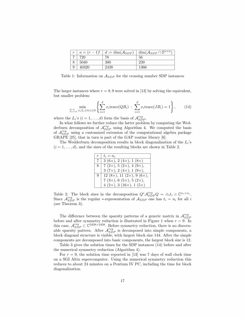
r n = (r − 1)! d := dim(ASDP ) dim(ASDP ∩ Sn×n)7 720 78 568 5040 380 2399 40320 2438 1366

Table 1: Information on ASDP for the crossing number SDP instances

The larger instances where r = 8, 9 were solved in [13] by solving the equivalent,but smaller problem:

min∑di=1 xiLi�0,x≥0

{d∑

i=1

xitrace(QBi) :d∑

i=1

xitrace(JBi) = 1

}, (14)

where the Li’s (i = 1, . . . , d) form the basis of AregSDP .

In what follows we further reduce the latter problem by computing the Wed-derburn decomposition of Areg

SDP using Algorithm 4. We computed the basisof Areg

SDP using a customized extension of the computational algebra packageGRAPE [25], that in turn is part of the GAP routine library [6].

The Wedderburn decomposition results in block diagonalization of the Li’s(i = 1, . . . , d), and the sizes of the resulting blocks are shown in Table 2.

r ti = ni

7 3 (6×), 2 (4×), 1 (8×)8 7 (2×), 5 (2×), 4 (9×),

3 (7×), 2 (4×), 1 (9×),9 12 (8×), 11 (2×), 9 (6×),

7 (3×), 6 (5×), 5 (2×),4 (2×), 3 (16×), 1 (5×)

Table 2: The block sizes in the decomposition Q∗AregSDP Q = ⊕iti � Cni×ni .

Since AregSDP is the regular ∗-representation of ASDP one has ti = ni for all i

(see Theorem 3).

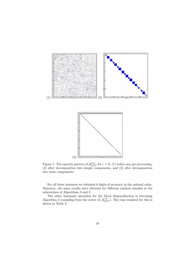
The difference between the sparsity patterns of a generic matrix in AregSDP

before and after symmetry reduction is illustrated in Figure 1 when r = 9. Inthis case, Areg

SDP ⊂ C2438×2438. Before symmetry reduction, there is no discern-able sparsity pattern. After Areg

SDP is decomposed into simple components, ablock diagonal structure is visible, with largest block size 144. After the simplecomponents are decomposed into basic components, the largest block size is 12.

Table 3 gives the solution times for the SDP instances (14) before and afterthe numerical symmetry reduction (Algorithm 4).

For r = 9, the solution time reported in [13] was 7 days of wall clock timeon a SGI Altix supercomputer. Using the numerical symmetry reduction thisreduces to about 24 minutes on a Pentium IV PC, including the time for blockdiagonalization.

17

(1) (2)

(3)

Figure 1: The sparsity pattern of AregSDP for r = 9: (1) before any pre-processing,

(2) after decomposition into simple components, and (3) after decompositioninto basic components.

For all three instances we obtained 6 digits of accuracy in the optimal value.Moreover, the same results were obtained for different random samples in thesubroutines of Algorithms 3 and 2.

The other dominant operation for the block diagonalization is executingAlgorithm 3 (sampling from the center of Areg

SDP ). The time required for this isshown in Table 3.

18

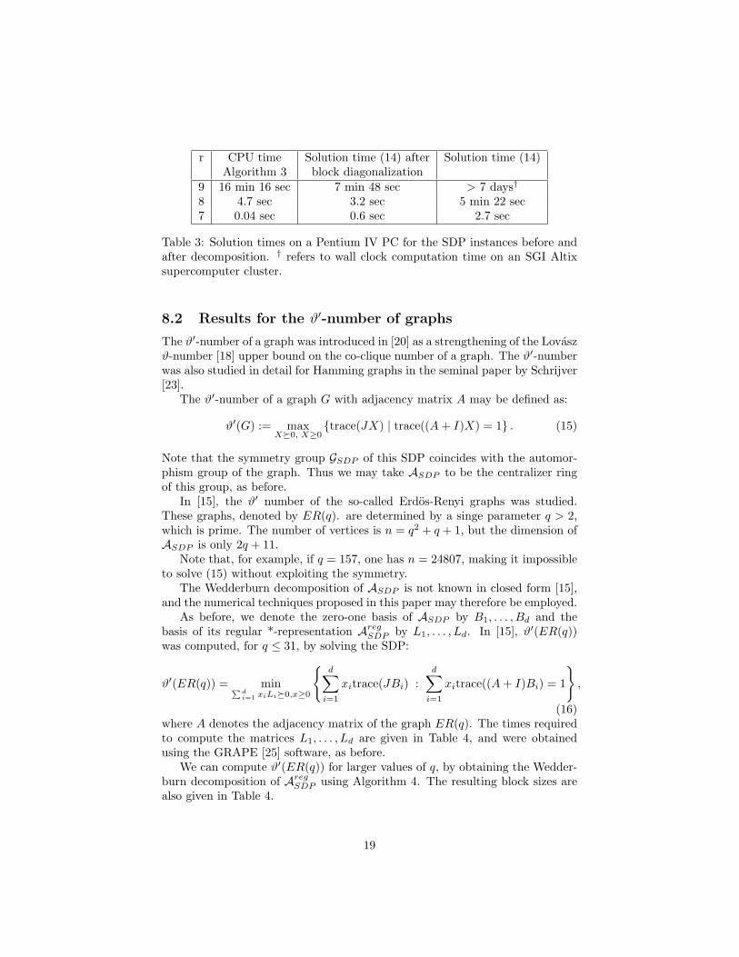
r CPU time Solution time (14) after Solution time (14)Algorithm 3 block diagonalization

9 16 min 16 sec 7 min 48 sec > 7 days†

8 4.7 sec 3.2 sec 5 min 22 sec7 0.04 sec 0.6 sec 2.7 sec

Table 3: Solution times on a Pentium IV PC for the SDP instances before andafter decomposition. † refers to wall clock computation time on an SGI Altixsupercomputer cluster.

8.2 Results for the ϑ′-number of graphs

The ϑ′-number of a graph was introduced in [20] as a strengthening of the Lovaszϑ-number [18] upper bound on the co-clique number of a graph. The ϑ′-numberwas also studied in detail for Hamming graphs in the seminal paper by Schrijver[23].

The ϑ′-number of a graph G with adjacency matrix A may be defined as:

ϑ′(G) := maxX�0, X≥0

{trace(JX) | trace((A + I)X) = 1} . (15)

Note that the symmetry group GSDP of this SDP coincides with the automor-phism group of the graph. Thus we may take ASDP to be the centralizer ringof this group, as before.

In [15], the ϑ′ number of the so-called Erdos-Renyi graphs was studied.These graphs, denoted by ER(q). are determined by a singe parameter q > 2,which is prime. The number of vertices is n = q2 + q + 1, but the dimension ofASDP is only 2q + 11.

Note that, for example, if q = 157, one has n = 24807, making it impossibleto solve (15) without exploiting the symmetry.

The Wedderburn decomposition of ASDP is not known in closed form [15],and the numerical techniques proposed in this paper may therefore be employed.

As before, we denote the zero-one basis of ASDP by B1, . . . , Bd and thebasis of its regular *-representation Areg

SDP by L1, . . . , Ld. In [15], ϑ′(ER(q))was computed, for q ≤ 31, by solving the SDP:

ϑ′(ER(q)) = min∑di=1 xiLi�0,x≥0

{d∑

i=1

xitrace(JBi) :d∑

i=1

xitrace((A + I)Bi) = 1

},

(16)where A denotes the adjacency matrix of the graph ER(q). The times requiredto compute the matrices L1, . . . , Ld are given in Table 4, and were obtainedusing the GRAPE [25] software, as before.

We can compute ϑ′(ER(q)) for larger values of q, by obtaining the Wedder-burn decomposition of Areg

SDP using Algorithm 4. The resulting block sizes arealso given in Table 4.

19

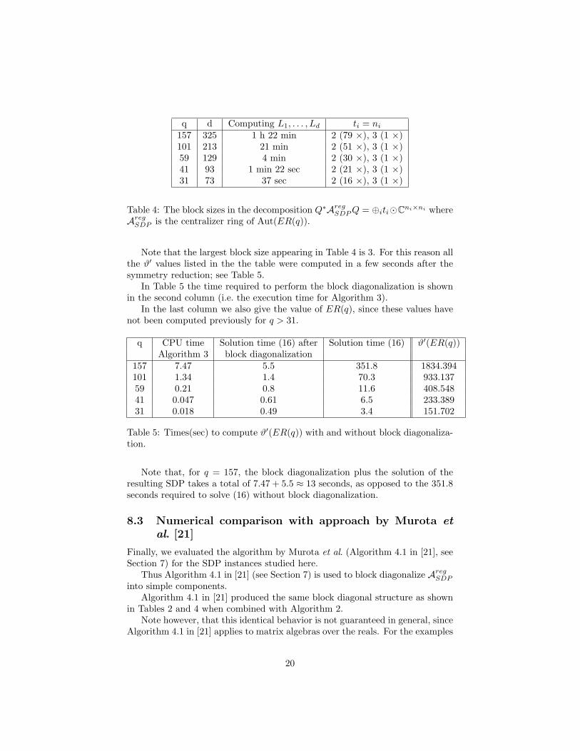
q d Computing L1, . . . , Ld ti = ni

157 325 1 h 22 min 2 (79 ×), 3 (1 ×)101 213 21 min 2 (51 ×), 3 (1 ×)59 129 4 min 2 (30 ×), 3 (1 ×)41 93 1 min 22 sec 2 (21 ×), 3 (1 ×)31 73 37 sec 2 (16 ×), 3 (1 ×)

Table 4: The block sizes in the decomposition Q∗AregSDP Q = ⊕iti�Cni×ni where

AregSDP is the centralizer ring of Aut(ER(q)).

Note that the largest block size appearing in Table 4 is 3. For this reason allthe ϑ′ values listed in the the table were computed in a few seconds after thesymmetry reduction; see Table 5.

In Table 5 the time required to perform the block diagonalization is shownin the second column (i.e. the execution time for Algorithm 3).

In the last column we also give the value of ER(q), since these values havenot been computed previously for q > 31.

q CPU time Solution time (16) after Solution time (16) ϑ′(ER(q))Algorithm 3 block diagonalization

157 7.47 5.5 351.8 1834.394101 1.34 1.4 70.3 933.13759 0.21 0.8 11.6 408.54841 0.047 0.61 6.5 233.38931 0.018 0.49 3.4 151.702

Table 5: Times(sec) to compute ϑ′(ER(q)) with and without block diagonaliza-tion.

Note that, for q = 157, the block diagonalization plus the solution of theresulting SDP takes a total of 7.47 + 5.5 ≈ 13 seconds, as opposed to the 351.8seconds required to solve (16) without block diagonalization.

8.3 Numerical comparison with approach by Murota etal. [21]

Finally, we evaluated the algorithm by Murota et al. (Algorithm 4.1 in [21], seeSection 7) for the SDP instances studied here.

Thus Algorithm 4.1 in [21] (see Section 7) is used to block diagonalize AregSDP

into simple components.Algorithm 4.1 in [21] produced the same block diagonal structure as shown

in Tables 2 and 4 when combined with Algorithm 2.Note however, that this identical behavior is not guaranteed in general, since

Algorithm 4.1 in [21] applies to matrix algebras over the reals. For the examples

20

studied here though, one could replace Algorithm 3 by Algorithm 4.1 in [21] inour Algorithm 4.

Acknowledgements

The authors are deeply indebted to Professor Masakazu Kojima for suggestingthe outline of the proof of Theorem 4, and for making his Matlab implementationof Algorithm 4.1 in [21] available to them.

The authors also thank an anonymous referee for pointing out erroneousnumerical results in an earlier version of this paper.

References

[1] F. Alizadeh. Combinatorial optimization with interior point methods andsemi–definite matrices. PhD thesis, University of Minnesota, Minneapolis,USA, 1991.

[2] C. Bachoc and F. Vallentin. New upper bounds for kissing numbers fromsemidefinite programming. Journal of the AMS, 21:909-924, 2008.

[3] Y.-Q. Bai, E. de Klerk, D.V. Pasechnik, and R. Sotirov. Exploiting groupsymmetry in truss topology optimization. Optimization and Engineering10(3):331–349, 2009.

[4] P.J. Cameron. Coherent configurations, association schemes, and permu-tation groups, pp. 55-71 in Groups, Combinatorics and Geometry (A. A.Ivanov, M. W. Liebeck and J. Saxl eds.), World Scientific, Singapore, 2003.

[5] W. Eberly and M. Giesbrecht. Efficient decomposition of separable alge-bras. Journal of Symbolic Computation, 37(1):35–81, 2004.

[6] GAP – Groups, Algorithms, and Programming, Version 4.4.12, TheGAP Group, 2008, http://www.gap-system.org

[7] K. Gatermann and P.A. Parrilo, Symmetry groups, semidefinite programs,and sums of squares. J. Pure and Applied Algebra, 192:95–128, 2004.

[8] D. Gijswijt. Matrix Algebras and Semidefinite Programming Techniquesfor Codes. PhD thesis, University of Amsterdam, The Netherlands, 2005.http://staff.science.uva.nl/~gijswijt/promotie/thesis.pdf

[9] D. Gijswijt, A. Schrijver, H. Tanaka, New upper bounds for nonbinarycodes based on the Terwilliger algebra and semidefinite programming, Jour-nal of Combinatorial Theory, Series A, 113:1719–1731, 2006.

[10] Y. Kanno, M. Ohsaki, K. Murota and N. Katoh. Group symmetry ininterior-point methods for semidefinite program, Optimization and Engi-neering, 2(3): 293–320, 2001.

21

[11] E. de Klerk. Exploiting special structure in semidefinite programming: asurvey of theory and applications. European Journal of Operational Re-search, 201(1): 1–10, 2010.

[12] E. de Klerk, J. Maharry, D.V. Pasechnik, B. Richter and G. Salazar. Im-proved bounds for the crossing numbers of Km,n and Kn. SIAM Journalon Discrete Mathematics 20:189–202, 2006.

[13] E. de Klerk, D.V. Pasechnik and A. Schrijver. Reduction of symmetricsemidefinite programs using the regular *-representation. MathematicalProgramming B, 109(2-3):613-624, 2007.

[14] E. de Klerk and R. Sotirov. Exploiting Group Symmetry in SemidefiniteProgramming Relaxations of the Quadratic Assignment Problem. Mathe-matical Programming, Series A, 122(2):225–246, 2010.

[15] E. de Klerk, M.W. Newman, D.V. Pasechnik, and R. Sotirov. On the Lovaszϑ-number of almost regular graphs with application to Erdos-Renyi graphs.European Journal of Combinatorics, 31:879–888, 2009.

[16] M. Kojima, S. Kojima and S. Hara. Linear algebra for semidefinite pro-gramming, Research Report B-290, Tokyo Institute of Technology, October1994; also in RIMS Kokyuroku 1004, Kyoto University, pp. 1-23, 1997.

[17] M. Laurent. Strengthened semidefinite bounds for codes. MathematicalProgramming, 109(2-3):239–261, 2007.

[18] L. Lovasz. On the Shannon capacity of a graph. IEEE Transactions onInformation theory, 25:1–7, 1979.

[19] T. Maehara and K. Murota. A numerical algorithm for block-diagonal de-composition of matrix *-algebras, Part II: general algorithm, May 2009,submitted for publication. (Original version: A numerical algorithm forblock-diagonal decomposition of matrix *-algebras with general irreduciblecomponents, METR 2008-26, University of Tokyo, May 2008.)

[20] R.J. McEliece, E.R. Rodemich, and H.C. Rumsey (1978), The Lovaszbound and some generalizations. Journal of Combinatorics, Information& System Sciences 3:134152, 1978.

[21] K. Murota, Y. Kanno, M. Kojima and S. Kojima, A Numerical Algorithmfor Block-Diagonal Decomposition of Matrix *-Algebras, Technical reportB-445, Department of Mathematical and Computing Sciences, Tokyo In-stitute of Technology, September 2007 (Revised June 2008).

[22] Yu.E. Nesterov and A.S. Nemirovski. Interior point polynomial algorithmsin convex programming. SIAM Studies in Applied Mathematics, Vol. 13.SIAM, Philadelphia, USA, 1994.

22

[23] A. Schrijver. A comparison of the Delsarte and Lovasz bounds. IEEE Trans-actions on Information Theory, 25:425–429, 1979.

[24] A. Schrijver. New code upper bounds from the Terwilliger algebra. IEEETransactions on Information Theory, 51:2859–2866, 2005.

[25] L.H. Soicher. GRAPE: GRaph Algorithms using PErmutation groups—A GAP package, Version number 4.3, 2006, http://www.maths.qmul.ac.uk/~leonard/grape/

[26] M.J. Todd. Semidefinite optimization. Acta Numerica, 10:515–560, 2001.

[27] K. C. Toh, M. J. Todd, and R. H. Tutuncu. SDPT3—a MATLAB softwarepackage for semidefinite programming, version 1.3. Optimization Methodsand Software, 11/12(1-4):545–581, 1999.

[28] F. Vallentin. Symmetry in semidefinite programs. Linear Algebra and itsApplications, to appear. Preprint version: arXiv:0706.4233

[29] L. Vandenberghe and S. Boyd. Semidefinite programming. SIAM Review,38:49–95, 1996.

[30] J.H.M. Wedderburn. On hypercomplex numbers. Proc. London Math. Soc.6(2):77–118, 1907.

[31] B. Weisfeiler, editor. On Construction and Identification of Graphs,Springer, Lecture Notes in Mathematics 558, 1976.

23