Numerical Integration - Wouter den Haan · Numerical Integration Wouter J. Den Haan London School of Economics c by Wouter J. Den Haan. OverviewNewton-CotesGaussian quadratureExtra

Numerical Integration

Wouter J. Den HaanLondon School of Economics

c© by Wouter J. Den Haan

Overview Newton-Cotes Gaussian quadrature Extra

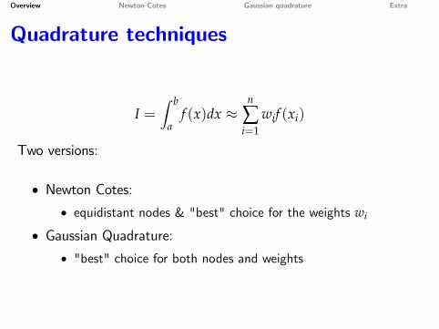
Quadrature techniques

I =∫ b

af (x)dx ≈

n

∑i=1

wif (xi) =n

∑i=1

wifi

• Nodes: xi

• Weights: wi


Quadrature techniques

I =∫ b

af (x)dx ≈

n

∑i=1

wif (xi)

Two versions:

• Newton Cotes:• equidistant nodes & "best" choice for the weights wi

• Gaussian Quadrature:• "best" choice for both nodes and weights


Monte Carlo techniques

• pseudo:• implemetable version of true Monte Carlo

• quasi:• looks like Monte Carlo, but is something different

• name should have been chosen better


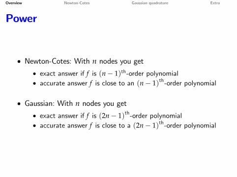
Power

• Newton-Cotes: With n nodes you get• exact answer if f is (n− 1)th-order polynomial• accurate answer f is close to an (n− 1)th-order polynomial

• Gaussian: With n nodes you get• exact answer if f is (2n− 1)th-order polynomial• accurate answer f is close to a (2n− 1)th-order polynomial


Power

• (Pseudo) Monte Carlo: accuracy requires lots of draws

• Quasi Monte Carlo: definitely better than (pseudo) MonteCarlo and dominates quadrature methods forhigher-dimensional problems


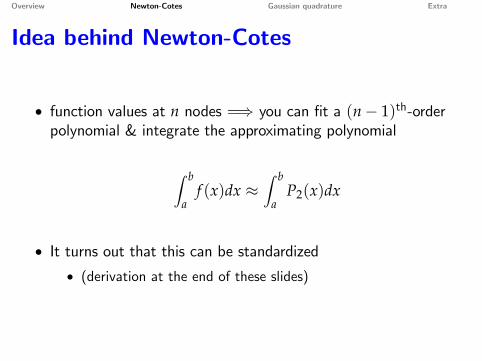
Idea behind Newton-Cotes

• function values at n nodes =⇒ you can fit a (n− 1)th-orderpolynomial & integrate the approximating polynomial

∫ b

af (x)dx ≈

∫ b

aP2(x)dx

• It turns out that this can be standardized• (derivation at the end of these slides)


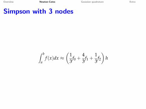
Simpson with 3 nodes

∫ b

af (x)dx ≈

(13

f0 +43

f1 +13

f2

)h


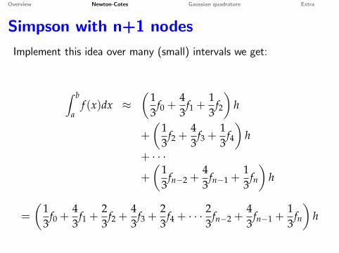
Simpson with n+1 nodesImplement this idea over many (small) intervals we get:

∫ b

af (x)dx ≈

(13

f0 +43

f1 +13

f2

)h

+

(13

f2 +43

f3 +13

f4

)h

+ · · ·

+

(13

fn−2 +43

fn−1 +13

fn

)h

=

(13

f0 +43

f1 +23

f2 +43

f3 +23

f4 + · · ·23

fn−2 +43

fn−1 +13

fn

)h


Simpson in Matlab

• Integration routine in Matlab

quad(@myfun,A,B)

• This is an adaptive procedure that adjusts the length of theinterval (by looking at changes in derivatives)


Gaussian quadrature

• Could we do better? That is, get better accuracy with sameamount of nodes?

• Answer: Yes, if you are smart about choosing the nodes• This is Gaussian quadrature


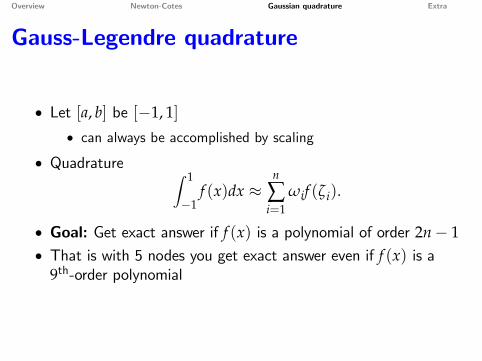
Gauss-Legendre quadrature

• Let [a, b] be [−1, 1]• can always be accomplished by scaling

• Quadrature ∫ 1

−1f (x)dx ≈

n

∑i=1

ωif (ζi).

• Goal: Get exact answer if f (x) is a polynomial of order 2n− 1• That is with 5 nodes you get exact answer even if f (x) is a

9th-order polynomial


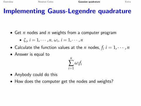
Implementing Gauss-Legendre quadrature

• Get n nodes and n weights from a computer program• ζ i, i = 1, · · · , n, ωi, i = 1, · · · , n

• Calculate the function values at the n nodes, fi i = 1, · · · , n• Answer is equal to

n

∑i=1

ωifi

• Anybody could do this• How does the computer get the nodes and weights?


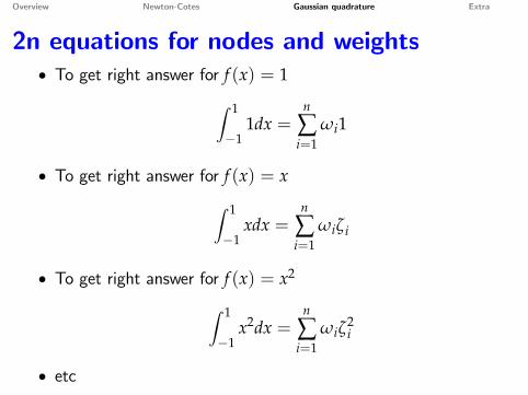
2n equations for nodes and weights• To get right answer for f (x) = 1∫ 1

−11dx =

n

∑i=1

ωi1

• To get right answer for f (x) = x∫ 1

−1xdx =

n

∑i=1

ωiζ i

• To get right answer for f (x) = x2

∫ 1

−1x2dx =

n

∑i=1

ωiζ2i

• etc


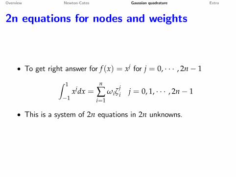
2n equations for nodes and weights

• To get right answer for f (x) = xj for j = 0, · · · , 2n− 1∫ 1

−1xjdx =

n

∑i=1

ωiζji j = 0, 1, · · · , 2n− 1

• This is a system of 2n equations in 2n unknowns.


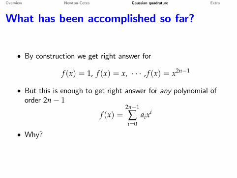
What has been accomplished so far?

• By construction we get right answer for

f (x) = 1, f (x) = x, · · · , f (x) = x2n−1

• But this is enough to get right answer for any polynomial oforder 2n− 1

f (x) =2n−1

∑i=0

aixi

• Why?


Gauss-Hermite Quadrature

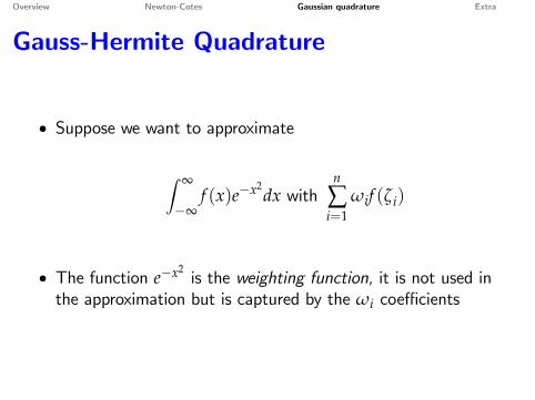
• Suppose we want to approximate

∫ ∞

−∞f (x)e−x2

dx withn

∑i=1

ωif (ζi)

• The function e−x2is the weighting function, it is not used in

the approximation but is captured by the ωi coeffi cients


Gauss-Hermite Quadrature

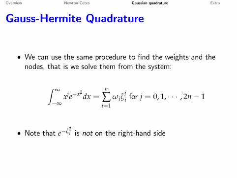
• We can use the same procedure to find the weights and thenodes, that is we solve them from the system:

∫ ∞

−∞xje−x2

dx =n

∑i=1

ωiζji for j = 0, 1, · · · , 2n− 1

• Note that e−ζ2i is not on the right-hand side


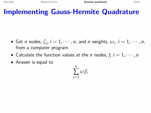
Implementing Gauss-Hermite Quadrature

• Get n nodes, ζi, i = 1, · · · , n, and n weights, ωi, i = 1, · · · , n,from a computer program

• Calculate the function values at the n nodes, fi i = 1, · · · , n• Answer is equal to

n

∑i=1

ωifi


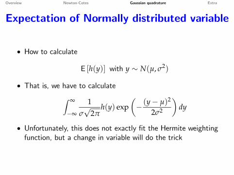
Expectation of Normally distributed variable

• How to calculate

E [h(y)] with y ∼ N(µ, σ2)

• That is, we have to calculate∫ ∞

−∞

1σ√

2πh(y) exp

(− (y− µ)2

2σ2

)dy

• Unfortunately, this does not exactly fit the Hermite weightingfunction, but a change in variable will do the trick


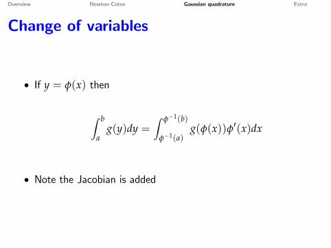
Change of variables

• If y = φ(x) then

∫ b

ag(y)dy =

∫ φ−1(b)

φ−1(a)g(φ(x))φ′(x)dx

• Note the Jacobian is added


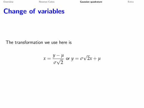
Change of variables

The transformation we use here is

x =y− µ

σ√

2or y = σ

√2x+ µ


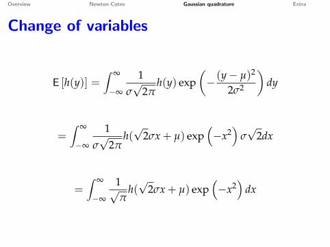
Change of variables

E [h(y)] =∫ ∞

−∞

1σ√

2πh(y) exp

(− (y− µ)2

2σ2

)dy

=∫ ∞

−∞

1σ√

2πh(√

2σx+ µ) exp(−x2

)σ√

2dx

=∫ ∞

−∞

1√π

h(√

2σx+ µ) exp(−x2

)dx


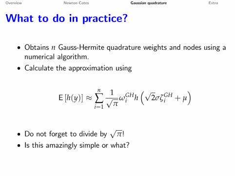
What to do in practice?

• Obtains n Gauss-Hermite quadrature weights and nodes using anumerical algorithm.

• Calculate the approximation using

E [h(y)] ≈n

∑i=1

1√π

ωGHi h

(√2σζGH

i + µ)

• Do not forget to divide by√

π!• Is this amazingly simple or what?


Extra material

• Derivation Simpson formula• Monte Carlo integration


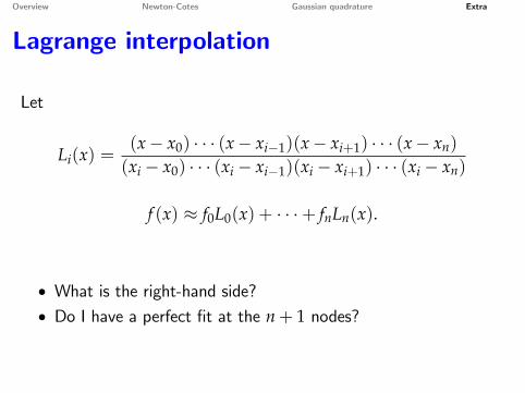
Lagrange interpolation

Let

Li(x) =(x− x0) · · · (x− xi−1)(x− xi+1) · · · (x− xn)

(xi − x0) · · · (xi − xi−1)(xi − xi+1) · · · (xi − xn)

f (x) ≈ f0L0(x) + · · ·+ fnLn(x).

• What is the right-hand side?• Do I have a perfect fit at the n+ 1 nodes?


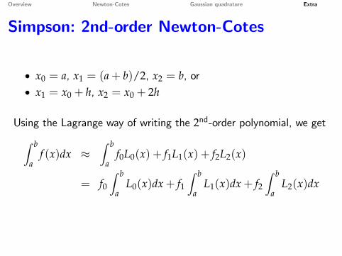
Simpson: 2nd-order Newton-Cotes

• x0 = a, x1 = (a+ b)/2, x2 = b, or• x1 = x0 + h, x2 = x0 + 2h

Using the Lagrange way of writing the 2nd-order polynomial, we get∫ b

af (x)dx ≈

∫ b

af0L0(x) + f1L1(x) + f2L2(x)

= f0∫ b

aL0(x)dx+ f1

∫ b

aL1(x)dx+ f2

∫ b

aL2(x)dx


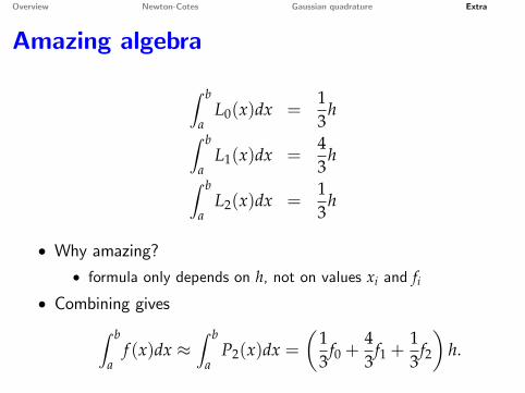
Amazing algebra

∫ b

aL0(x)dx =

13

h∫ b

aL1(x)dx =

43

h∫ b

aL2(x)dx =

13

h

• Why amazing?• formula only depends on h, not on values xi and fi

• Combining gives∫ b

af (x)dx ≈

∫ b

aP2(x)dx =

(13

f0 +43

f1 +13

f2

)h.


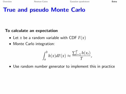
True and pseudo Monte Carlo

To calculate an expectation

• Let x be a random variable with CDF F(x)• Monte Carlo integration:∫ b

ah(x)dF(x) ≈ ∑T

t=1 h(xt)

T,

• Use random number generator to implement this in practice


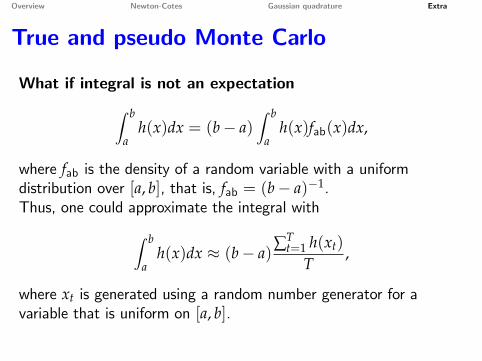
True and pseudo Monte Carlo

What if integral is not an expectation∫ b

ah(x)dx = (b− a)

∫ b

ah(x)fab(x)dx,

where fab is the density of a random variable with a uniformdistribution over [a, b], that is, fab = (b− a)−1.Thus, one could approximate the integral with∫ b

ah(x)dx ≈ (b− a)∑T

t=1 h(xt)

T,

where xt is generated using a random number generator for avariable that is uniform on [a, b].


Quasi Monte Carlo

• Monte Carlo integration has very slow convergence properties• In higher dimensional problems, however, it does better thanquadrature (it seems to avoid the curse of dimensionality)

• But why? Pseudo MC is simply a deterministic way to gothrough the state space

• Quasi MC takes that idea and improves upon it


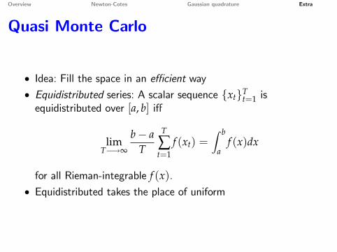
Quasi Monte Carlo

• Idea: Fill the space in an effi cient way• Equidistributed series: A scalar sequence {xt}T

t=1 isequidistributed over [a, b] iff

limT−→∞

b− aT

T

∑t=1

f (xt) =∫ b

af (x)dx

for all Rieman-integrable f (x).• Equidistributed takes the place of uniform


Quasi Monte Carlo

.

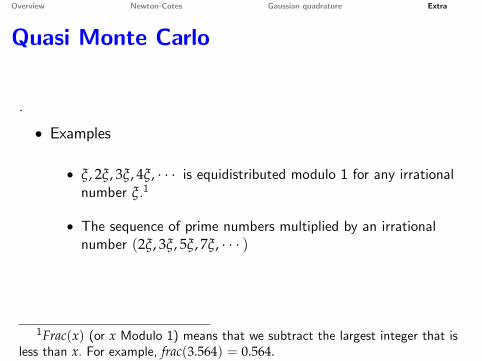
• Examples

• ξ, 2ξ, 3ξ, 4ξ, · · · is equidistributed modulo 1 for any irrationalnumber ξ.1

• The sequence of prime numbers multiplied by an irrationalnumber (2ξ, 3ξ, 5ξ, 7ξ, · · · )

1Frac(x) (or x Modulo 1) means that we subtract the largest integer that isless than x. For example, frac(3.564) = 0.564.


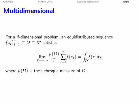
Multidimensional

For a d-dimensional problem, an equidistributed sequence{xt}T

t=1 ⊂ D ⊂ Rd satisfies

limT−→∞

µ(D)T

T

∑t=1

f (xt) =∫

Df (x)dx,

where µ(D) is the Lebesque measure of D.


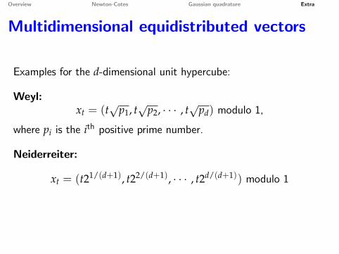
Multidimensional equidistributed vectors

Examples for the d-dimensional unit hypercube:

Weyl:xt = (t

√p1, t√

p2, · · · , t√

pd) modulo 1,

where pi is the ith positive prime number.

Neiderreiter:

xt = (t21/(d+1), t22/(d+1), · · · , t2d/(d+1)) modulo 1


References

• Den Haan, W.J., Numerical Integration, online lecture notes.• Heer, B., and A. Maussner, 2009, Dynamic General EquilibriumModeling.

• Judd, K. L., 1998, Numerical Methods in Economics.• Miranda, M.J, and P.L. Fackler, 2002, Applied ComputationalEconomics and Finance.

Documents

Numerical Integration - Wouter den Haan · Numerical Integration Wouter J. Den Haan London School of Economics c by Wouter J. Den Haan. OverviewNewton-CotesGaussian quadratureExtra