Numerical investigation of the flow in a swirl generator, using

Numerical investigation of the flow in a swirlgenerator, using OpenFOAM

Master’s Thesis in Fluid Mechanics

OSCAR BERGMAN

Department of Applied MechanicsDivision of Fluid MechanicsCHALMERS UNIVERSITY OF TECHNOLOGYGoteborg, Sweden 2010Master’s Thesis 2010:25

MASTER’S THESIS 2010:25

Numerical investigation of the flow in a swirl generator,

using OpenFOAM

Master’s Thesis in Fluid MechanicsOSCAR BERGMAN

Department of Applied MechanicsDivision of Fluid Mechanics

CHALMERS UNIVERSITY OF TECHNOLOGY

Goteborg, Sweden 2010

Numerical investigation of the flow in a swirl generator, using OpenFOAMOSCAR BERGMAN

c©OSCAR BERGMAN, 2010

Master’s Thesis 2010:25ISSN 1652-8557Department of Applied MechanicsDivision of Fluid MechanicsChalmers University of TechnologySE-412 96 GoteborgSwedenTelephone: + 46 (0)31-772 1000

Chalmers ReproserviceGoteborg, Sweden 2010

Numerical investigation of the flow in a swirl generator, using OpenFOAMMaster’s Thesis in Fluid MechanicsOSCAR BERGMANDepartment of Applied MechanicsDivision of Fluid MechanicsChalmers University of Technology

Abstract

This work presents results from OpenFOAM simulations conducted on a swirl generatordesigned to give similar flow conditions to those of a Francis turbine operating at partialload. Francis turbines are one of the most commonly used water turbines. In these tur-bines, there is however a frequent problem occuring at part load. Due to a swirling flowin the draft tube, a transient helical vortex rope builds up and creates severe pressurefluctuations in the system that increase the risk for fatique. To predict and control suchflow features is therefore critical. A test rig was developed at the ”Politehnica” Universityof Timisoara, Romania, to provide a detailed experimental database of such flow features.This test rig has four parts: leaning strout vanes, stay vanes, a rotating runner which isdesigned to have zero torque, and a convergent divergent draft tube.

In this work, numerical results are compared and validated against measurements real-ized on the swirling flow test rig at the Polytechnica University of Timisoara in Romania.The computational mesh is created with ICEM-Hexa and the parts have been meshedseparately and then merged together, using General Grid Interfaces (GGI) to couple themnumerically. The finite volume method is used to solve both the unsteady and steady stateReynolds Averaged Navier Stokes equations and the standard k-ε model is used to closethe turbulence equations. Steady-state simulations is a preliminary method, which is lesstime-consuming and predicts the general behavior of the flow field. It also provides goodinitial conditions for the unsteady simulations. For the unsteady simulations, the mesh ofthe rotating part of the domain is rotating and the coupling between the stationary androtating parts is handled by a sliding GGI interface.

The simulation results shows a developing vortex rope in the draft tube which gives riseto oscillations of flow properties in the system. The size and shape of this vortex rope, aswell as the frequency of the oscillations it gives rise to, is highly dependent on the rota-tional speed of the free runner. The results show that a rotational speed of 920 rpm onthe runner, corresponds best with the measurements out of the three rotational speeds 870rpm, 890 rpm and 920 rpm. The rotational speed of 870 rpm gives a positive moment onthe runner, an rpm of 890 of almost zero moment, and a speed of 920 rpm gives a positivemoment on the runner. Fourier analysis of the pressure fluctuations show that several newfrequencies has been introduced compared to a previous OpenFOAM study which was onlymade on the draft tube. The main frequencies for a rotational speed of 920 rpm have beenestimated to 3.0 Hz corresponding to an extraction/retraction of the vortex rope, 18.02 Hzwhich comes from the rotation of the vortex rope and 153.19 Hz which is caused by therotor stator interaction. Furthermore, the amplitudes of the fourier spectra have showngood agreement with the previous study.

, Applied Mechanics, Master’s Thesis 2010:25 I

II , Applied Mechanics, Master’s Thesis 2010:25

Contents

Abstract I

Preface V

Aknowledgements V

1 Introduction 11.1 Experimental rig . . . . . . . . . . . . . . . . . . . . . . . . . . . . . . . . 21.2 Measurements . . . . . . . . . . . . . . . . . . . . . . . . . . . . . . . . . . 31.3 Previous studies . . . . . . . . . . . . . . . . . . . . . . . . . . . . . . . . . 3

2 Theory 52.1 Governing Equations . . . . . . . . . . . . . . . . . . . . . . . . . . . . . . 5

2.1.1 Reynolds-Averaged Navier-Stokes equations (RANS) . . . . . . . . 52.1.2 Eddy viscosity models . . . . . . . . . . . . . . . . . . . . . . . . . 62.1.3 k − ε turbulence model . . . . . . . . . . . . . . . . . . . . . . . . . 6

2.2 Computational Fluid Dynamics . . . . . . . . . . . . . . . . . . . . . . . . 7

3 Method 83.1 Description of the OpenFOAM CFD toolbox . . . . . . . . . . . . . . . . . 83.2 Numerical Setup . . . . . . . . . . . . . . . . . . . . . . . . . . . . . . . . 9

3.2.1 Steady-State simulations . . . . . . . . . . . . . . . . . . . . . . . . 93.2.2 Unsteady Simulations . . . . . . . . . . . . . . . . . . . . . . . . . . 10

4 Results and Discussion 104.1 Steady-State Simulations . . . . . . . . . . . . . . . . . . . . . . . . . . . . 10

4.1.1 Comparison with theoretical design profiles . . . . . . . . . . . . . . 114.1.2 Comparison with LDV measurements . . . . . . . . . . . . . . . . . 124.1.3 Comparing moment forces . . . . . . . . . . . . . . . . . . . . . . . 14

4.2 Unsteady Simulations . . . . . . . . . . . . . . . . . . . . . . . . . . . . . . 154.2.1 Comparison with theoretical design profiles . . . . . . . . . . . . . . 154.2.2 Comparison with LDV measurements . . . . . . . . . . . . . . . . . 164.2.3 Comparison between the PISO based solver and a SIMPLE based

solver . . . . . . . . . . . . . . . . . . . . . . . . . . . . . . . . . . 184.2.4 Comparison of moment forces and pressure fluctuations . . . . . . . 19

4.3 Fourier Analysis . . . . . . . . . . . . . . . . . . . . . . . . . . . . . . . . . 224.3.1 Fourier analysis theory . . . . . . . . . . . . . . . . . . . . . . . . . 224.3.2 Fourier algorithm in Matlab . . . . . . . . . . . . . . . . . . . . . . 234.3.3 Results of fourier analysis . . . . . . . . . . . . . . . . . . . . . . . 24

5 Conclusion 27

6 Future work 27

, Applied Mechanics, Master’s Thesis 2010:25 III

IV , Applied Mechanics, Master’s Thesis 2010:25

Preface

In this study the swirling flow of a swirl generator has been analyzed and numerically in-vestigated. The OpenFOAM software has been tested and validated against experiments.The work has been carried out from January 2010 to June 2010 at the Department of Ap-plied Mechanics Division of Fluid Mechanics Chalmers University of Technology, Sweden,with Oscar Bergman as student and with Olivier Petit and Professor Hakan Nilsson fromthe department of Applied Mechanics as supervisors.

Acknowledgements

I would like to acknowledge the Timisoara research group, Professor Romeo F.Susan-Resiga, Sebastian Muntean, Alan Bosioc and their team for sharing experimental resultswith me. I would also like to acknowledge the Swedish National Infrastructure for Comput-ing (SNIC) and Chalmers Center for Computational Science and Engineering (C3SE) forproviding computer resources. I would like to give my thanks to Andreo Gonzalez, ShashaXie, Xin Zhao and everyone else at the department of Applied Mechanics for creating anice working atmosphere. Also I would like to thank my girlfriend Elin Holstensson andmy parents Ove and Elisabeth Bergman for all love, patience and support. Finally I wantto thank my supervisors Hakan Nilsson and Olivier Petit for being very patient and forsharing their knowledge. They really made this project a stimulating and fun learningexperience.

Goteborg, April 2010Oscar Bergman

, Applied Mechanics, Master’s Thesis 2010:25 V

VI , Applied Mechanics, Master’s Thesis 2010:25

1 Introduction

Sweden has a good access to water power. With the Norwegian mountains in the north-west, the rivers through Sweden provide the way for the water to reach Ostersjon. Duringspring, the snow melts on the mountaintops and the water finds its way to the surface ofthe ocean. Almost all electric energy in Sweden is supplied by water power and nuclearpower. These days however, when a lot of resources are put to alternative energy sources,water turbines are often turned on and off and used for filling in when the energy demandis high. Wind power is for example sensitive to weather, and can often fail to deliver thepower quota which it is set to provide, thus creating a gap in the electric grid. During theconditions of starting and stopping the water turbines, an unwanted phenomenon occurs.Some of the water turbines used today are Francis turbines. They are radial and mixedflow turbines. When these turbines operate at partial load, the flow in the draft tube getsa swirling flow profile. This is due to the fact that the runner is designed to neutralize theswirl created by the guide vanes at the best efficiency point. If the turbine is operatingaway from the effiency point, this swirl will not be neutralized to the same extent. Thismay then cause a transient helical vortex rope to build up and create pressure fluctuationswhich greatly increases the risk of fatigue damage on the turbines. Solving this problem iscrucial, and knowing more about the flow features of a swirling flow will help developmentof techniques that can prevent these problems to occur.

This work presents numerical investigations of a swirl generator test rig installed at thePolytehnica University of Timisoara, Romania. The swirl generator is designed to givesimilar flow features to that of a Francis turbine operating at part load. That is, at certainflow discharge, a vortex rope builds up and creates pressure fluctuations which affects thestresses on the runner. The swirl generator consists of strout blades, stayvanes, a freerunner and a convergent divergent draft tube.

Figure 1.1: A precessing vortex rope, created by the swirling flow in the test rig.

Figure 1.1 shows the phenomenon which is studied in this work. A precessing helicalvortex rope caused by the flow conditions created in the swirl generator.

, Applied Mechanics, Master’s Thesis 2010:25 1

1.1 Experimental rig

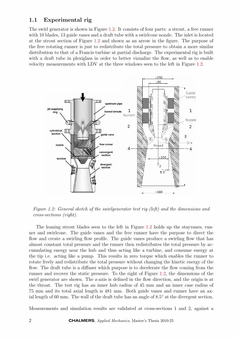
The swirl generator is shown in Figure 1.2. It consists of four parts: a strout, a free runnerwith 10 blades, 13 guide vanes and a draft tube with a swirlcone nozzle. The inlet is locatedat the strout section of Figure 1.2 and shown as an arrow in the figure. The purpose ofthe free rotating runner is just to redistribute the total pressure to obtain a more similardistribution to that of a Francis turbine at partial discharge. The experimental rig is builtwith a draft tube in plexiglass in order to better vizualize the flow, as well as to enablevelocity measurements with LDV at the three windows seen to the left in Figure 1.2.

Figure 1.2: General sketch of the swirlgenerator test rig (left) and the dimensions andcross-sections (right).

The leaning strout blades seen to the left in Figure 1.2 holds up the stayvanes, run-ner and swirlcone. The guide vanes and the free runner have the purpose to direct theflow and create a swirling flow profile. The guide vanes produce a swirling flow that hasalmost constant total pressure and the runner then redistributes the total pressure by ac-cumulating energy near the hub and thus acting like a turbine, and consume energy atthe tip i.e. acting like a pump. This results in zero torque which enables the runner torotate freely and redistribute the total pressure without changing the kinetic energy of theflow. The draft tube is a diffuser which purpose is to decelerate the flow coming from therunner and recover the static pressure. To the right of Figure 1.2, the dimensions of theswirl generator are shown. The z-axis is defined in the flow direction, and the origin is atthe throat. The test rig has an inner hub radius of 45 mm and an inner case radius of75 mm and its total axial length is 481 mm. Both guide vanes and runner have an ax-ial length of 60 mm. The wall of the draft tube has an angle of 8.5◦ at the divergent section.

Measurements and simulation results are validated at cross-sections 1 and 2, against a

2 , Applied Mechanics, Master’s Thesis 2010:25

theoretical design model, which was used when designing the swirl generator. The cross-sections are seen in the right of Figure 1.2. Cross-section 1 is located between the stay vanesand the runner and cross-section 2 is located just downstream the runner. Cross-sections3 and 4 are not used in this work.

1.2 Measurements

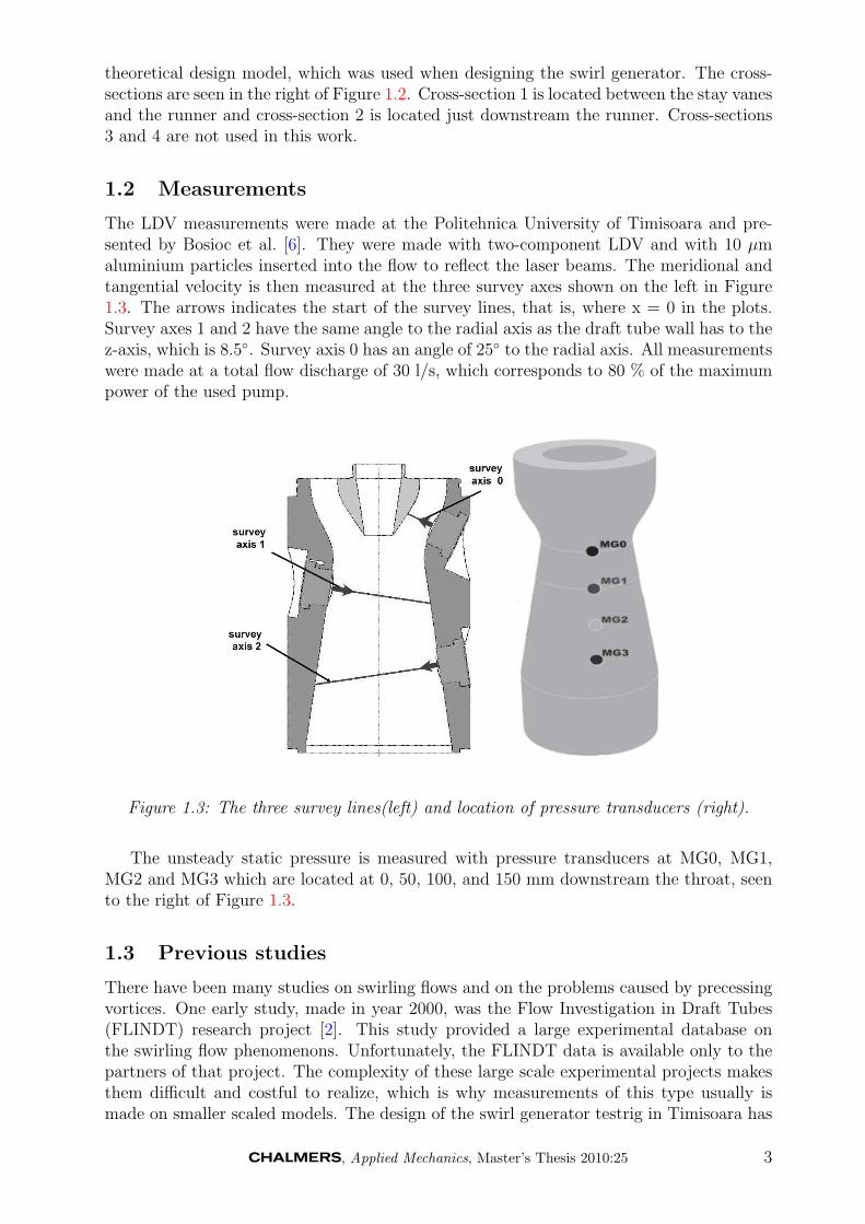
The LDV measurements were made at the Politehnica University of Timisoara and pre-sented by Bosioc et al. [6]. They were made with two-component LDV and with 10 µmaluminium particles inserted into the flow to reflect the laser beams. The meridional andtangential velocity is then measured at the three survey axes shown on the left in Figure1.3. The arrows indicates the start of the survey lines, that is, where x = 0 in the plots.Survey axes 1 and 2 have the same angle to the radial axis as the draft tube wall has to thez-axis, which is 8.5◦. Survey axis 0 has an angle of 25◦ to the radial axis. All measurementswere made at a total flow discharge of 30 l/s, which corresponds to 80 % of the maximumpower of the used pump.

Figure 1.3: The three survey lines(left) and location of pressure transducers (right).

The unsteady static pressure is measured with pressure transducers at MG0, MG1,MG2 and MG3 which are located at 0, 50, 100, and 150 mm downstream the throat, seento the right of Figure 1.3.

1.3 Previous studies

There have been many studies on swirling flows and on the problems caused by precessingvortices. One early study, made in year 2000, was the Flow Investigation in Draft Tubes(FLINDT) research project [2]. This study provided a large experimental database onthe swirling flow phenomenons. Unfortunately, the FLINDT data is available only to thepartners of that project. The complexity of these large scale experimental projects makesthem difficult and costful to realize, which is why measurements of this type usually ismade on smaller scaled models. The design of the swirl generator testrig in Timisoara has


similar goals to that of the FLINDT project. The optimal number of blades have beenestimated for creating similar swirling profiles to that of Francis turbines at part load,and the dimensions of the stay vanes and runner blades have been designed using a quasi-3D inverse design method for turbomachinery blades [15] to create a precessing vortexrope [16]. The convergent divergent draft tube have been designed with a beneficial shapefor swirling flows [5] and 2D Laser Doppler Velometry measurements have been made forinvestigating the flow at different parts of the swirl generator. Resiga [17] introduced atechnique to control the instabilities by using axial jet control in the discharge cone. Inlater studies [10], it was shown that at a jet discharge corresponding to 10% of the totalturbine discharge neutralizes the pressure oscillations the most. Muntean and Resiga laterconfirmed this in a 3D unsteady numerical investigation [4]. Using this technique wouldhowever require a to large fraction of the discharging flow to be bypassed, so Resiga andMuntean later showed that such a jet control can instead be obtained by using a flowfeedback method downstream the cone [14]. In a study by Muntean et al. [11], only thedraft tube was used when simulating the unsteady flow in 3D. Petit [13] extended thestudies by including all parts of the swirl generator test rig, which makes the draft tubeinlet conditions different from those applied by Muntean et al. [11]. This project aims atcreating a database of simulation results which can be used for further studies in attemptsto solve this problem.


2 Theory

When numerically simulating a flow field, the techniques and methods for this can be ofmany different kinds. The most used technique is based on the finite volume method whichuses small control volumes to discretise the governing differential equations.

2.1 Governing Equations

The equations that describe a fluid in motion are derived from the conservation of mass,momentum and energy. The motion of an incompressible fluid is described by the Navier-Stokes equations, which state that changes in momentum of a fluid only depends on thesurrounding pressure and the internal viscous fources acting on the fluid:

ρ

(∂ui∂t

+ vj∂ui∂xj

)︸︷︷︸

ρDuiDt

= − ∂p

∂xi+

∂

∂xj

(µ

(∂ui∂xj

+∂uj∂xi

))+ ρfi (2.1)

Where ρ is the density, DDt

the material derivative, u is the velocity, t is time, p is the staticpressure, µ is the dynamic viscosity and f is the body force acting on the fluid. Bodyforces can be for example gravity, centrifugal or Coriolis forces.

The Navier-Stokes equations are complemented with the continuity equations, which isa statement of conservation of mass:

∂ρ

∂t+∂ρuj∂xj

= 0 (2.2)

Dealing with water, this equations can be simplified due to the assumption of incompress-ibility, which means that density is independent of the pressure, and so the continuityequation becomes:

∂uj∂xj

= 0 (2.3)

Inserting into the Navier-Stokes equations we get:

ρ

(∂ui∂t

+ vj∂ui∂xj

)= − ∂p

∂xi+ µ

∂2ui∂x2

j

+ ρfi (2.4)

where the first term from the left is the unsteady term, the second term is the convectionterm. The sum of these two represents the inertia of the fluid. The third is the pressuregradient, the fourth is the viscosity term, and the last is again body forces acting on thefluid. Body forces like centrifugal or Coriolis forces appear when solving the equations ina rotating frame of reference.

2.1.1 Reynolds-Averaged Navier-Stokes equations (RANS)

The Reynolds-Averaged Navier-Stokes equations are the time averaged equations of theNavier-Stokes equations. They are obtained by decomposing the instantenous velocityvectors into one averaged part and one fluctuation part , i.e.

u(x, t) = U(x) + u′(x, t) (2.5)

inserting into the Navier-Stokes equations and time averaging yields :

ρ∂UjUi∂xj

= ρfi +∂

∂xj

[−P δij + µ

(∂Ui∂xj

+∂Uj∂xi

)− ρu′iu′j

](2.6)


In the unsteady RANS equations, an additional time dependant term is added on the lefthand side: ρ∂Ui

∂t.

As this averaging is performed, the new term u′iu′j appears. This is the Reynolds stress

tensor. It is an additional symmetric stress tensor that is added due to turbulence andwhich represents the correlations between fluctuating velocities. This stress tensor is un-known and it makes the system of equations unsolvable, as we have more unknowns thanequations. The equations can then be closed using a turbulence model for the Reynoldsstresses.

2.1.2 Eddy viscosity models

In eddy viscosity models, the closure problem is solved by introducing a linkage betweenthe Reynolds stresses and the velocity gradients, using an eddy viscocity µt. The diffusionterm then becomes:

∂

∂xj

[µ

(∂Ui∂xj

+∂Uj∂xi

)− ρu′iu′j

]=

∂

∂xj

[(µ+ µt)

(∂Ui∂xj

+∂Uj∂xi

)](2.7)

which gives us

ρu′iu′j = −µt

(∂Ui∂xj

+∂Uj∂xi

)(2.8)

if we set i=j, the reynolds stress becomes

u′iu′j ≡ 2k (2.9)

where k is the turbulent kinetic energy. Setting i=j however, the continuity equation wouldimply that u′iu

′j = 0. So in order to set i=j, we need to add 2/3ρδi,jk to the equation, i.e.

u′iu′j = −µt

(∂Ui∂xj

+∂Uj∂xi

)+

2

3ρδi,jk (2.10)

This relation is called the Boussinesq Assumption and the idea of this is to model thesmall-scale eddies with a viscosity term, similar to the way the momentum friction forcesin a fluid are modeled with a molecular viscosity.

2.1.3 k − ε turbulence model

The k−ε turbulence model is a two-equation eddy viscosity model that uses two transportequations to represent the turbulent properties of the flow. The equation of turbulentkinetic energy is derived from the Navier-Stokes equation. It includes convection terms,production terms, turbulent diffusion terms and dissipation. The turbulent dissipationterm ε, represents the transformation of kinetic energy at smaller scales into internal en-ergy. However, there are many unknowns in the k-equation, dissipation being one amongstthem. And so the k-equation is complemented with the dissipation-equation.

Turbulent kinetic energy-equation:

∂(ρk)

∂t+∂ρkUj∂xj

=∂

∂xj

[(µ+

µtσk

)∂k

∂xj

]+ Pk − ρε (2.11)

Dissipation -equation:

∂(ρε)

∂t+∂(ρεUj)

∂xj=

∂

∂xj

[(µ+

µtσε

)∂ε

∂xj

]+ C1ε

ε

kPk − C2ερ

ε2

k(2.12)


µt = ρCµk2

ε, Pk = −ρu′iu′j

∂uj∂xi

= µt2SijSij, Sij =1

2

(∂Ui∂xj

+∂Uj∂xi

)Here we have µt as the eddy viscosity and Pk as the production of turbulent kinetic energy.The model constants are given by:

C1ε = 1.44, C2ε = 1.92, Cµ = 0.09, σk = 1.0, σε = 1.3

The k-ε model uses wall functions to resolve the turbulence close to the wall. The meshis thus generated to give y+ values in the range from 30 to 300. The k − ε model is astable turbulence model which often is referred to as the industry standard model. Thedownsides can be that it is bad at predicting normal stresses which means that it can’ttake effects of streamline curvature into account or predict stagnation flows.

2.2 Computational Fluid Dynamics

Computational Fluid Dynamics (CFD), is nowadays an important tool for simulating flowsof all kinds. In the finite volume method the computational domain is divided into a largenumber of control volumes. The general transport equation

∂ρφ

∂t+∇ · (ρuφ) = ∇ · (Γ∇φ) + Sφ (2.13)

with φ beeing the quantity needed, ρ the density, u the velocities, Γ is a diffusivity constantand Sφ is a source term. Integrated over each control volume (CV) and time interval ∆t,it can be rewritten using Gauss’s divergence theorem to a surface integral:∫ t+∆t

t

[∫CV

∂ρφ

∂tdV +

∫A

ρu · ndA]dt =

∫ t+∆t

t

[∫A

Γ∇φ · ndA+

∫CV

SφdV

]dt (2.14)

where n is an outward pointing unit normal of the boundary of the control volume. Thefirst term on the left hand side represents the rate of change of the fluid property φ inthe control volume and the second term represents the net rate transport of property φout of the volume due to convection. The first term on the right hand side is the net ratetransport of property φ into the control volume due to diffusion and the last term on theright hand side is the net rate of increase of φ due to sources inside the control volume.

In order to then solve the equations, a discretisation of the different terms is needed.This discretisation can be done in different ways, dependent on the physics of the termbeing discretized. The convection term could for example be discretized with a range ofdifferent schemes such as the second order central differencing scheme, first and secondorder upwind scheme etc.. These schemes are just ways to interpolate the information thatis being transported between the cells and the order of each discretization scheme is just ameasure of its efficiency and accuracy.

As there is no explicit pressure equation included in the calculations, some type of pro-cedure is needed to couple the pressure with the velocity equations. The SIMPLE andPISO algorithms are methods of dealing with this. These procedures are well covered inliterature [18].


3 Method

The case setup is based on the swirl generator developed and created at the Polytech-nica University of Timisoara in Romania. A mesh was created with the dimensions of thetest rig, and then both steady and unsteady simulations were conducted using the Open-FOAM CFD toolbox. The results were later viewed in the visual tool kit Paraview andpostprocessed using Matlab and the two free softwares Gnuplot and Octave.

3.1 Description of the OpenFOAM CFD toolbox

OpenFOAM is an open source CFD software that has the advantage of beeing open forchanges and development. The users can contribute with new ideas and help with ex-tending the software features. OpenFOAM consists of a C++ library, which foremost isused to create applications. These applications consist of solvers and utilities. The solversare used for solving continuum mechanics problems, and the utilities are mostly used tomanipulate data in different forms. The main advantage with OpenFOAM however, is theease with which you can create and customize solvers. The solver applications are writtenwith OpenFOAM classes, which simplifies the syntax to resemble the partial differentialequations that is being used. To be able to make this happen, the programming languageneeds to have properties such as inheritance, template classes, virtual functions and oper-ator overloading. This is not found in many languages except for a few such as C++ andFortran-90 [1].

The solvers and utilities are controlled through the use of dictionaries. These are fileswhere specifications of the applications are accessed and controlled. Specificiations suchas disctretisations methods, Courant number, start and end time, divergence scheme, tur-bulenced method, pressure corrector settings, linear solver settings and many more are allcontrolled and accessed through these sets of dictionaries. Running the solvers in parallell,on several processors simultaneously, is done by decomposing the case into as many parts asprocessors intended for the job. This is easily done in OpenFOAM with the decomposeParutility. This utility is also controlled by a dictionary where you can specify in which wayto decompose your computational mesh.When the solver is finally running it will initiate the computations with the values givenin a folder named 0, as in time 0. Then it will print the quantity fields in time folders,with a time interval specified in the dictionary controlDict. Residuals are printed in theprompt during computations unless they are specified to be logged in a log file. When thesimulations are finished, the case can be reconstructed with the utility reconstructPar andpostprocessed through the VTK visualization application paraFoam.


3.2 Numerical Setup

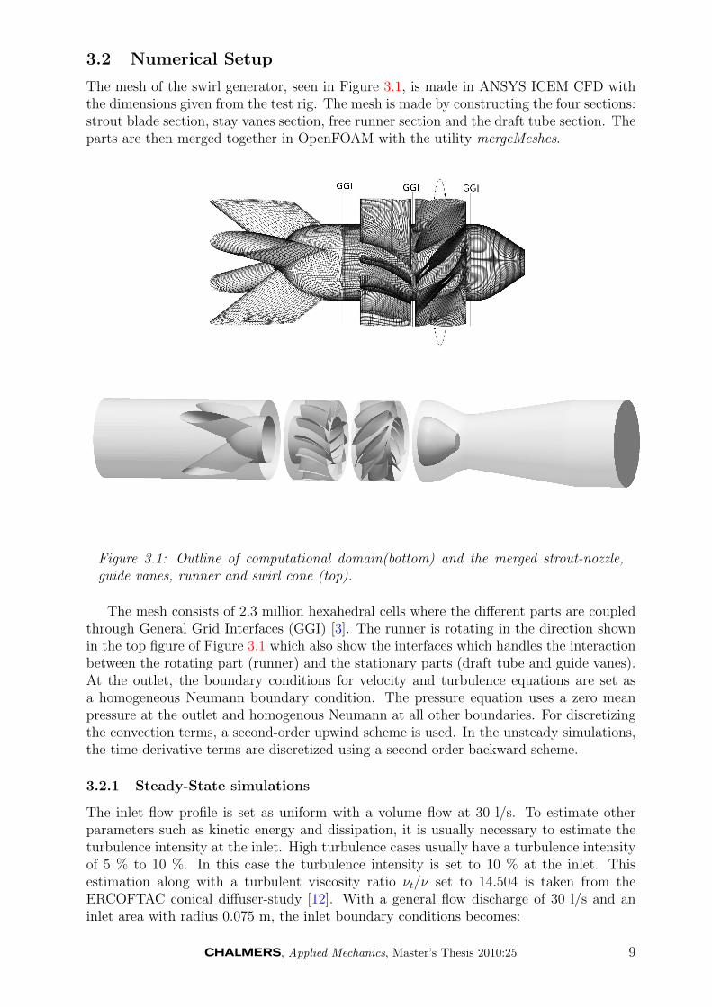
The mesh of the swirl generator, seen in Figure 3.1, is made in ANSYS ICEM CFD withthe dimensions given from the test rig. The mesh is made by constructing the four sections:strout blade section, stay vanes section, free runner section and the draft tube section. Theparts are then merged together in OpenFOAM with the utility mergeMeshes.

Figure 3.1: Outline of computational domain(bottom) and the merged strout-nozzle,guide vanes, runner and swirl cone (top).

The mesh consists of 2.3 million hexahedral cells where the different parts are coupledthrough General Grid Interfaces (GGI) [3]. The runner is rotating in the direction shownin the top figure of Figure 3.1 which also show the interfaces which handles the interactionbetween the rotating part (runner) and the stationary parts (draft tube and guide vanes).At the outlet, the boundary conditions for velocity and turbulence equations are set asa homogeneous Neumann boundary condition. The pressure equation uses a zero meanpressure at the outlet and homogenous Neumann at all other boundaries. For discretizingthe convection terms, a second-order upwind scheme is used. In the unsteady simulations,the time derivative terms are discretized using a second-order backward scheme.

3.2.1 Steady-State simulations

The inlet flow profile is set as uniform with a volume flow at 30 l/s. To estimate otherparameters such as kinetic energy and dissipation, it is usually necessary to estimate theturbulence intensity at the inlet. High turbulence cases usually have a turbulence intensityof 5 % to 10 %. In this case the turbulence intensity is set to 10 % at the inlet. Thisestimation along with a turbulent viscosity ratio νt/ν set to 14.504 is taken from theERCOFTAC conical diffuser-study [12]. With a general flow discharge of 30 l/s and aninlet area with radius 0.075 m, the inlet boundary conditions becomes:


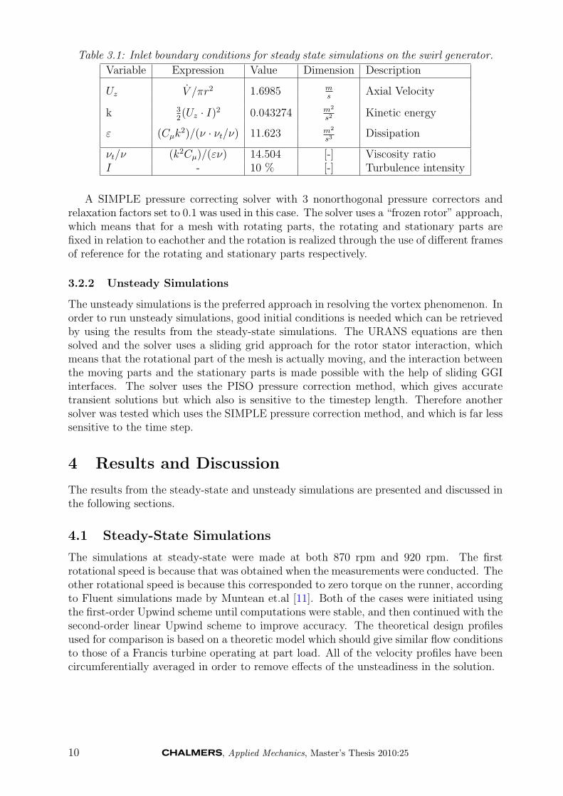
Table 3.1: Inlet boundary conditions for steady state simulations on the swirl generator.

Variable Expression Value Dimension Description

Uz V /πr2 1.6985 ms

Axial Velocity

k 32(Uz · I)2 0.043274 m2

s2Kinetic energy

ε (Cµk2)/(ν · νt/ν) 11.623 m2

s3Dissipation

νt/ν (k2Cµ)/(εν) 14.504 [-] Viscosity ratioI - 10 % [-] Turbulence intensity

A SIMPLE pressure correcting solver with 3 nonorthogonal pressure correctors andrelaxation factors set to 0.1 was used in this case. The solver uses a “frozen rotor” approach,which means that for a mesh with rotating parts, the rotating and stationary parts arefixed in relation to eachother and the rotation is realized through the use of different framesof reference for the rotating and stationary parts respectively.

3.2.2 Unsteady Simulations

The unsteady simulations is the preferred approach in resolving the vortex phenomenon. Inorder to run unsteady simulations, good initial conditions is needed which can be retrievedby using the results from the steady-state simulations. The URANS equations are thensolved and the solver uses a sliding grid approach for the rotor stator interaction, whichmeans that the rotational part of the mesh is actually moving, and the interaction betweenthe moving parts and the stationary parts is made possible with the help of sliding GGIinterfaces. The solver uses the PISO pressure correction method, which gives accuratetransient solutions but which also is sensitive to the timestep length. Therefore anothersolver was tested which uses the SIMPLE pressure correction method, and which is far lesssensitive to the time step.

4 Results and Discussion

The results from the steady-state and unsteady simulations are presented and discussed inthe following sections.

4.1 Steady-State Simulations

The simulations at steady-state were made at both 870 rpm and 920 rpm. The firstrotational speed is because that was obtained when the measurements were conducted. Theother rotational speed is because this corresponded to zero torque on the runner, accordingto Fluent simulations made by Muntean et.al [11]. Both of the cases were initiated usingthe first-order Upwind scheme until computations were stable, and then continued with thesecond-order linear Upwind scheme to improve accuracy. The theoretical design profilesused for comparison is based on a theoretic model which should give similar flow conditionsto those of a Francis turbine operating at part load. All of the velocity profiles have beencircumferentially averaged in order to remove effects of the unsteadiness in the solution.


4.1.1 Comparison with theoretical design profiles

0

0.1

0.2

0.3

0.4

0.5

0.6

0.7

0.8

0.045 0.05 0.055 0.06 0.065 0.07 0.075

Dim

ensi

onle

ss v

eloc

ity [-

]

Radius [m]

Numerical meridional velocity at 920 rpmNumerical meridional velocity at 870 rpm

Theoretical meridional velocity 0

0.1

0.2

0.3

0.4

0.5

0.6

0.7

0.045 0.05 0.055 0.06 0.065 0.07 0.075

Dim

ensi

onle

ss v

eloc

ity [-

]

Radius [m]

Numerical tangential velocity at 920 rpmNumerical tangential velocity at 870 rpm

Theoretical tangential velocity

0

0.2

0.4

0.6

0.8

1

1.2

0.045 0.05 0.055 0.06 0.065 0.07 0.075

Dim

ensi

onle

ss v

eloc

ity [-

]

Radius [m]

Numerical meridional velocity at 920 rpmNumerical meridional velocity at 870 rpm


0.1

0.2

0.3

0.4

0.5

0.6

0.7

0.045 0.05 0.055 0.06 0.065 0.07 0.075

Dim

ensi

onle

ss v

eloc

ity [-

]

Radius [m]

Numerical tangential velocity at 920 rpmNumerical tangential velocity at 870 rpm


Figure 4.1: Meridional (left) and tangential (right) velocities at cross-sections 1 (top)and 2 (bottom), compared with the theoretical design profile for each section.

Figure 4.1 show the velocity profiles at cross-sections 1 and 2, with section 1 locatedbetween the guide vanes and the runner and section 2 located downstream the runner.The results are compared with the theoretical design profiles from the blade design studyby Resiga et.al [15]. The numerical results show a good agreement with the design profiles.In the case with a rotational speed of 870 rpm, the tangential velocity at cross-section2 is in good agreement with the theoretical design profile. However, it is not reachingits intended value near the shroud, and in the case of 920 rpm, the tangential velocity isoverestimated compared to the theoretical profile design. This means that a rotationalspeed of 920 rpm is too high and that 870 rpm will more accurately create a swirling flowthat corresponds to the flow estimated by the theoretical model. As seen in Figure 4.1,the two numerical velocity profiles show a very similar shape to eachother. This similarityindicates that the deviation at the shroud is not dependent of the rotational speed, andthat it’s more likely caused by the computational model.


4.1.2 Comparison with LDV measurements

Comparison with LDV measurements for both rotational speeds is shown in Figure 4.2.The data is presented in dimensionless values where the used references are the minimumradius of the throat and the mean velocity at the throat. (see Figure 1.3 to see where thelocation of the survey axes are)

Rthroat = 0.05 [m], vthroat =V

π ·R2throat

[m/s]

-2

-1.5

-1

-0.5

0

0.5

1

1.5

2

0 0.1 0.2 0.3 0.4 0.5 0.6

Dim

ensi

onle

ss v

eloc

ity [-

]

Dimensionless survey axis [-]

Measured meridional velocityMeasured tangential velocity

Numerical meridional velocityNumerical tangential velocity

-2

-1.5

-1

-0.5

0

0.5

1

1.5

2

0 0.1 0.2 0.3 0.4 0.5 0.6

Dim

ensi

onle

ss v

eloc

ity [-

]




-1.5

-1

-0.5

0

0.5

1

1.5

0 0.5 1 1.5 2

Dim

ensi

onle

ss v

eloc

ity [-

]




-1.5

-1

-0.5

0

0.5

1

1.5

0 0.5 1 1.5 2

Dim

ensi

onle

ss v

eloc

ity [-

]




-1

-0.5

0

0.5

1

0 0.5 1 1.5 2 2.5

Dim

ensi

onle

ss v

eloc

ity [-

]




-1

-0.5

0

0.5

1

0 0.5 1 1.5 2 2.5

Dim

ensi

onle

ss v

eloc

ity [-

]




Figure 4.2: Comparison with meridional and tangential velocities between simulationsat 870 rpm (left) and 920 rpm (right). Velocities are compared at survey axis 0 (topplots), survey axis 1 (middle plots), and survey axis 2 (bottom plots).


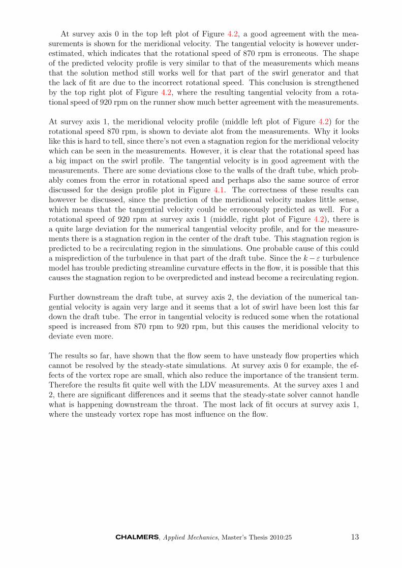
At survey axis 0 in the top left plot of Figure 4.2, a good agreement with the mea-surements is shown for the meridional velocity. The tangential velocity is however under-estimated, which indicates that the rotational speed of 870 rpm is erroneous. The shapeof the predicted velocity profile is very similar to that of the measurements which meansthat the solution method still works well for that part of the swirl generator and thatthe lack of fit are due to the incorrect rotational speed. This conclusion is strengthenedby the top right plot of Figure 4.2, where the resulting tangential velocity from a rota-tional speed of 920 rpm on the runner show much better agreement with the measurements.

At survey axis 1, the meridional velocity profile (middle left plot of Figure 4.2) for therotational speed 870 rpm, is shown to deviate alot from the measurements. Why it lookslike this is hard to tell, since there’s not even a stagnation region for the meridional velocitywhich can be seen in the measurements. However, it is clear that the rotational speed hasa big impact on the swirl profile. The tangential velocity is in good agreement with themeasurements. There are some deviations close to the walls of the draft tube, which prob-ably comes from the error in rotational speed and perhaps also the same source of errordiscussed for the design profile plot in Figure 4.1. The correctness of these results canhowever be discussed, since the prediction of the meridional velocity makes little sense,which means that the tangential velocity could be erroneously predicted as well. For arotational speed of 920 rpm at survey axis 1 (middle, right plot of Figure 4.2), there isa quite large deviation for the numerical tangential velocity profile, and for the measure-ments there is a stagnation region in the center of the draft tube. This stagnation region ispredicted to be a recirculating region in the simulations. One probable cause of this coulda misprediction of the turbulence in that part of the draft tube. Since the k− ε turbulencemodel has trouble predicting streamline curvature effects in the flow, it is possible that thiscauses the stagnation region to be overpredicted and instead become a recirculating region.

Further downstream the draft tube, at survey axis 2, the deviation of the numerical tan-gential velocity is again very large and it seems that a lot of swirl have been lost this fardown the draft tube. The error in tangential velocity is reduced some when the rotationalspeed is increased from 870 rpm to 920 rpm, but this causes the meridional velocity todeviate even more.

The results so far, have shown that the flow seem to have unsteady flow properties whichcannot be resolved by the steady-state simulations. At survey axis 0 for example, the ef-fects of the vortex rope are small, which also reduce the importance of the transient term.Therefore the results fit quite well with the LDV measurements. At the survey axes 1 and2, there are significant differences and it seems that the steady-state solver cannot handlewhat is happening downstream the throat. The most lack of fit occurs at survey axis 1,where the unsteady vortex rope has most influence on the flow.


4.1.3 Comparing moment forces

0.1118

0.1119

0.112

0.1121

0.1122

0.1123

0.1124

90000 100000 110000 120000 130000 140000

Mom

ent [

Nm

]

Iteration [-]

-0.5542

-0.554

-0.5538

-0.5536

-0.5534

-0.5532

-0.553

40000 50000 60000 70000 80000 90000 100000

Mom

ent [

Nm

]

Iterations [-]

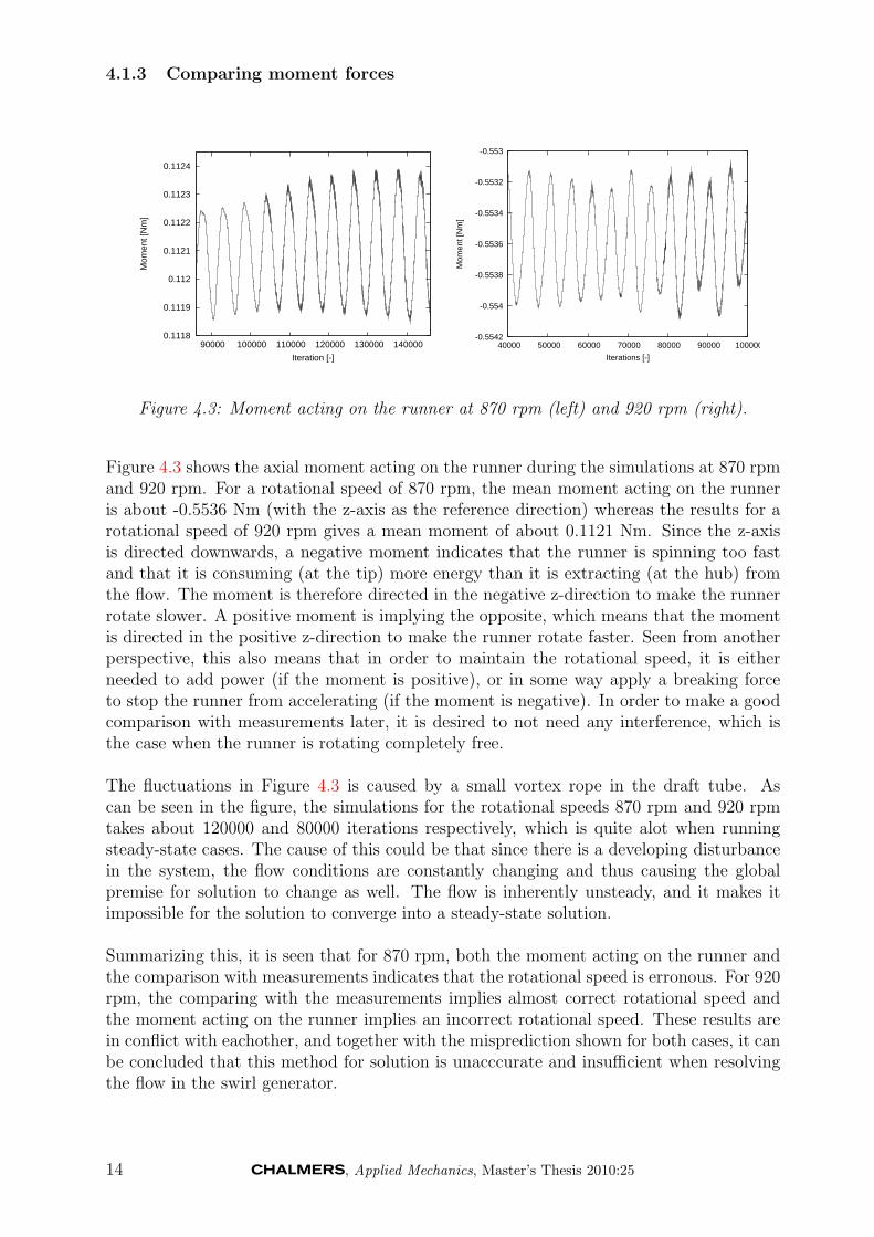
Figure 4.3: Moment acting on the runner at 870 rpm (left) and 920 rpm (right).

Figure 4.3 shows the axial moment acting on the runner during the simulations at 870 rpmand 920 rpm. For a rotational speed of 870 rpm, the mean moment acting on the runneris about -0.5536 Nm (with the z-axis as the reference direction) whereas the results for arotational speed of 920 rpm gives a mean moment of about 0.1121 Nm. Since the z-axisis directed downwards, a negative moment indicates that the runner is spinning too fastand that it is consuming (at the tip) more energy than it is extracting (at the hub) fromthe flow. The moment is therefore directed in the negative z-direction to make the runnerrotate slower. A positive moment is implying the opposite, which means that the momentis directed in the positive z-direction to make the runner rotate faster. Seen from anotherperspective, this also means that in order to maintain the rotational speed, it is eitherneeded to add power (if the moment is positive), or in some way apply a breaking forceto stop the runner from accelerating (if the moment is negative). In order to make a goodcomparison with measurements later, it is desired to not need any interference, which isthe case when the runner is rotating completely free.

The fluctuations in Figure 4.3 is caused by a small vortex rope in the draft tube. Ascan be seen in the figure, the simulations for the rotational speeds 870 rpm and 920 rpmtakes about 120000 and 80000 iterations respectively, which is quite alot when runningsteady-state cases. The cause of this could be that since there is a developing disturbancein the system, the flow conditions are constantly changing and thus causing the globalpremise for solution to change as well. The flow is inherently unsteady, and it makes itimpossible for the solution to converge into a steady-state solution.

Summarizing this, it is seen that for 870 rpm, both the moment acting on the runner andthe comparison with measurements indicates that the rotational speed is erronous. For 920rpm, the comparing with the measurements implies almost correct rotational speed andthe moment acting on the runner implies an incorrect rotational speed. These results arein conflict with eachother, and together with the misprediction shown for both cases, it canbe concluded that this method for solution is unacccurate and insufficient when resolvingthe flow in the swirl generator.


4.2 Unsteady Simulations

The solver for the unsteady simulations uses the feature of a sliding grid to simulate therotor stator interaction and the PISO algorithm for coupling the pressure with the velocityequations. The simulations are made at a rotational speed of 870 rpm, 920 rpm and 890rpm, where 890 rpm is obtained from linear interpolation of the results of 870 rpm and920 rpm. A solver which uses the SIMPLE algorithm is tested and compared to the PISObased solver. The initial conditions for all cases, are taken from the results of the steadystate simulations. For the case at 890 rpm, the steady-state results from the 870 rpmsimulations was used.

The simulations at 870 rpm were realized using a time step of 1.3e-4 s, yielding a maximumCourant number of 2.79. For the simulations with 920 rpm and 890 rpm, the timestep was1.4e-4 s and 1.2e-4 s respectively, giving a maximum Courant number of 3 at 920 rpm and2.5 at 890 rpm. The numerical velocity profiles are all averaged circumferentially and intime.

4.2.1 Comparison with theoretical design profiles

0

0.1

0.2

0.3

0.4

0.5

0.6

0.7

0.8

0.045 0.05 0.055 0.06 0.065 0.07 0.075

Dim

ensi

onle

ss v

eloc

ity [-

]

Radius [m]

Numerical meridional velocity at 920 rpmNumerical meridional velocity at 870 rpmNumerical meridional velocity at 890 rpm


0.1

0.2

0.3

0.4

0.5

0.6

0.7

0.045 0.05 0.055 0.06 0.065 0.07 0.075

Dim

ensi

onle

ss v

eloc

ity [-

]

Radius [m]

Numerical tangential velocity at 920 rpmNumerical tangential velocity at 870 rpmNumerical tangential velocity at 890 rpm


0

0.2

0.4

0.6

0.8

1

1.2

0.045 0.05 0.055 0.06 0.065 0.07 0.075

Dim

ensi

onle

ss v

eloc

ity [-

]

Radius [m]

Numerical meridional velocity at 920 rpmNumerical meridional velocity at 870 rpmNumerical meridional velocity at 890 rpm


0.1

0.2

0.3

0.4

0.5

0.6

0.7

0.045 0.05 0.055 0.06 0.065 0.07 0.075

Dim

ensi

onle

ss v

eloc

ity [-

]

Radius [m]

Numerical tangential velocity at 920 rpmNumerical tangential velocity at 870 rpmNumerical tangential velocity at 890 rpm


Figure 4.4: Meridional (left) and tangential (right) velocities at cross-sections 1 (top)and 2 (bottom), compared with the theoretical design profile for each section.

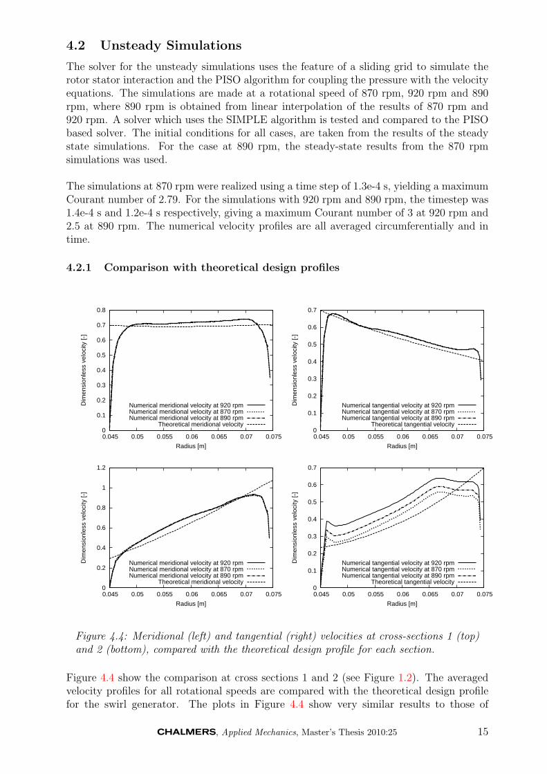
Figure 4.4 show the comparison at cross sections 1 and 2 (see Figure 1.2). The averagedvelocity profiles for all rotational speeds are compared with the theoretical design profilefor the swirl generator. The plots in Figure 4.4 show very similar results to those of


the steady-state simulations. The numerical velocity profiles are in good agreement withthe theoretical design profiles and the tangential velocities at cross-section 2 are againdeviating close to the shroud. The fact that the velocity profiles show these similaritieswith the steady-state results means that unsteady effects in this part of the flow is verysmall, and so the unsteady term in the equations gives little change to the solution. Asfor the steady-state results, simulation with the rotational speed of 870 rpm gives the bestagreement. When the rotational speed is increased, so is also the error in tangential speed.

4.2.2 Comparison with LDV measurements

-2

-1.5

-1

-0.5

0

0.5

1

1.5

2

0 0.1 0.2 0.3 0.4 0.5 0.6

Dim

ensi

onle

ss v

eloc

ity [-

]




-2

-1.5

-1

-0.5

0

0.5

1

1.5

2

0 0.1 0.2 0.3 0.4 0.5 0.6

Dim

ensi

onle

ss v

eloc

ity [-

]




-1.5

-1

-0.5

0

0.5

1

1.5

0 0.5 1 1.5 2

Dim

ensi

onle

ss v

eloc

ity [-

]




-1.5

-1

-0.5

0

0.5

1

1.5

0 0.5 1 1.5 2

Dim

ensi

onle

ss v

eloc

ity [-

]




-1

-0.5

0

0.5

1

0 0.5 1 1.5 2 2.5

Dim

ensi

onle

ss v

eloc

ity [-

]




-1

-0.5

0

0.5

1

0 0.5 1 1.5 2 2.5

Dim

ensi

onle

ss v

eloc

ity [-

]




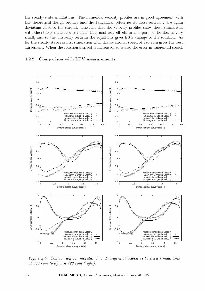
Figure 4.5: Comparison for meridional and tangential velocities between simulationsat 870 rpm (left) and 920 rpm (right).


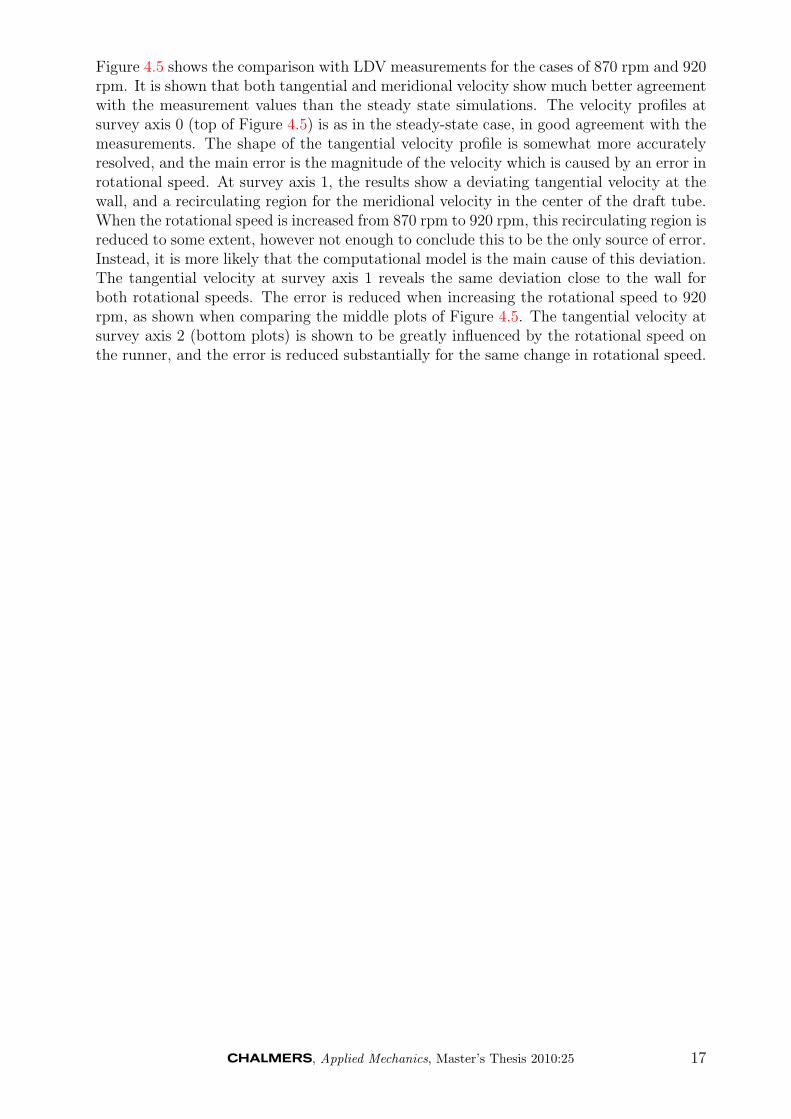
Figure 4.5 shows the comparison with LDV measurements for the cases of 870 rpm and 920rpm. It is shown that both tangential and meridional velocity show much better agreementwith the measurement values than the steady state simulations. The velocity profiles atsurvey axis 0 (top of Figure 4.5) is as in the steady-state case, in good agreement with themeasurements. The shape of the tangential velocity profile is somewhat more accuratelyresolved, and the main error is the magnitude of the velocity which is caused by an error inrotational speed. At survey axis 1, the results show a deviating tangential velocity at thewall, and a recirculating region for the meridional velocity in the center of the draft tube.When the rotational speed is increased from 870 rpm to 920 rpm, this recirculating region isreduced to some extent, however not enough to conclude this to be the only source of error.Instead, it is more likely that the computational model is the main cause of this deviation.The tangential velocity at survey axis 1 reveals the same deviation close to the wall forboth rotational speeds. The error is reduced when increasing the rotational speed to 920rpm, as shown when comparing the middle plots of Figure 4.5. The tangential velocity atsurvey axis 2 (bottom plots) is shown to be greatly influenced by the rotational speed onthe runner, and the error is reduced substantially for the same change in rotational speed.


4.2.3 Comparison between the PISO based solver and a SIMPLE based solver

-2

-1.5

-1

-0.5

0

0.5

1

1.5

2

0 0.1 0.2 0.3 0.4 0.5 0.6

Dim

ensi

onle

ss v

eloc

ity [-

]


Meridial velocity PISOTangential velocity PISOMeridial velocity SIMPLE

Tangential velocity SIMPLE-2

-1.5

-1

-0.5

0

0.5

1

1.5

2

0 0.1 0.2 0.3 0.4 0.5 0.6

Dim

ensi

onle

ss v

eloc

ity [-

]


Measured meridional velocityMeasured tangential velocityMeridional velocity SIMPLETangential velocity SIMPLE

-1.5

-1

-0.5

0

0.5

1

1.5

0 0.5 1 1.5 2

Dim

ensi

onle

ss v

eloc

ity [-

]



Tangential velocity SIMPLE-1.5

-1

-0.5

0

0.5

1

1.5

0 0.5 1 1.5 2

Dim

ensi

onle

ss v

eloc

ity [-

]



-1

-0.5

0

0.5

1

0 0.5 1 1.5 2 2.5

Dim

ensi

onle

ss v

eloc

ity [-

]



Tangential velocity SIMPLE-1

-0.5

0

0.5

1

0 0.5 1 1.5 2 2.5

Dim

ensi

onle

ss v

eloc

ity [-

]



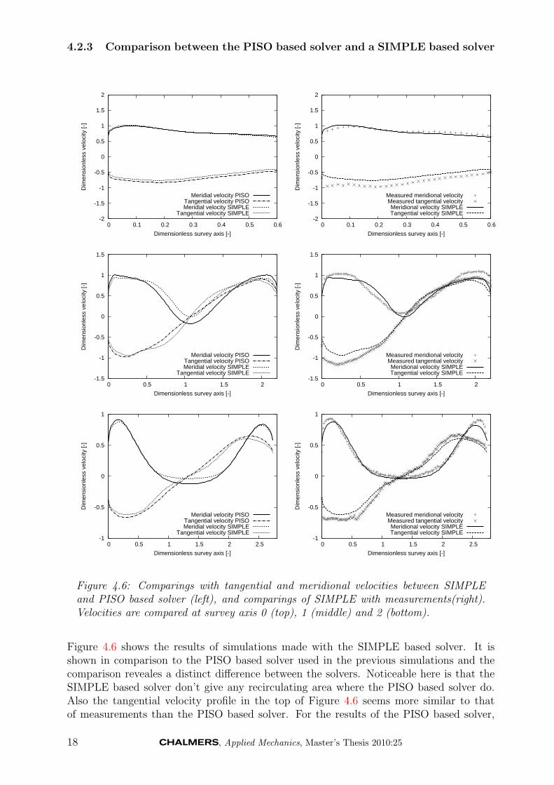
Figure 4.6: Comparings with tangential and meridional velocities between SIMPLEand PISO based solver (left), and comparings of SIMPLE with measurements(right).Velocities are compared at survey axis 0 (top), 1 (middle) and 2 (bottom).

Figure 4.6 shows the results of simulations made with the SIMPLE based solver. It isshown in comparison to the PISO based solver used in the previous simulations and thecomparison reveales a distinct difference between the solvers. Noticeable here is that theSIMPLE based solver don’t give any recirculating area where the PISO based solver do.Also the tangential velocity profile in the top of Figure 4.6 seems more similar to thatof measurements than the PISO based solver. For the results of the PISO based solver,


the tangential velocity in the center part of the draft tube looks more like a straight line,and it seems that the solver don’t predict this “s”-shape, shown in the measurements.The SIMPLE based solver seems to be resolving this. The comparison with measurementsdownstream the throat, at survey axis 1 and 2, show a very good agreement. There isstill a deviation close to the wall, but this has been concluded to be caused by an errorin rotational speed rather than the computational model, which makes these results thebest so far. The SIMPLE method for coupling the pressure with the velocity equationsare usually considered the more stable method out of the two. This stability is oftenachieved at the expense of accuracy, and so the results from using this method shouldbe less accurate than using PISO. The results are interesting, but further investigation isneeded in order to conclude that the SIMPLE based solver really gives a better predictionand that these results are not caused by “inaccuracy“ instead of accuracy.

4.2.4 Comparison of moment forces and pressure fluctuations

0.338

0.339

0.34

0.341

0.342

0.343

0.344

0.345

0.346

0.347

1.87 1.88 1.89 1.9 1.91 1.92 1.93 1.94 1.95

Mom

ent [

Nm

]

Time [s]

-0.298

-0.297

-0.296

-0.295

-0.294

-0.293

-0.292

-0.291

-0.29

1.89 1.9 1.91 1.92 1.93 1.94 1.95 1.96 1.97

Mom

ent [

Nm

]

Time [s]

0.082

0.084

0.086

0.088

0.09

0.092

0.094

1.86 1.87 1.88 1.89 1.9 1.91 1.92 1.93 1.94

Mom

ent [

Nm

]

Time [s]

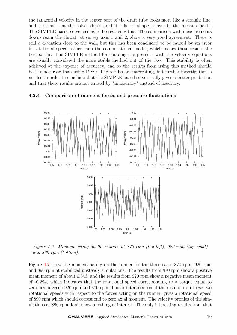
Figure 4.7: Moment acting on the runner at 870 rpm (top left), 920 rpm (top right)and 890 rpm (bottom).

Figure 4.7 show the moment acting on the runner for the three cases 870 rpm, 920 rpmand 890 rpm at stabilized unsteady simulations. The results from 870 rpm show a positivemean moment of about 0.343, and the results from 920 rpm show a negative mean momentof -0.294, which indicates that the rotational speed corresponding to a torque equal tozero lies between 920 rpm and 870 rpm. Linear interpolation of the results from these tworotational speeds with respect to the forces acting on the runner, gives a rotational speedof 890 rpm which should correspond to zero axial moment. The velocity profiles of the sim-ulations at 890 rpm don’t show anything of interest. The only interesting results from that


simulation is the moment acting on the runner, shown in the bottom plot in Figure 4.7. Itis seen that for 890 rpm, the mean moment acting on the runner is approximately 0.088Nm. This is not sufficient to conclude that 890 rpm is the correct rotational speed, but itis however a close value and it should give very similar flow conditions as the rotationalspeed that do give a torque equal to zero. The rotational speed could be better estimateddoing one additional linear interpolation, or maybe use another method to pinpoint wherethe moment will be zero.

Several frequencies can be observed in the plots of Figure 4.7. At least 3 frequenciescan be seen: One low frequency, one intermediate frequency and one high frequency whichall are caused by the pressure fluctuations in the system. Therefore, the pressure is anal-ysed in the following section to see where these frequencies originates from.

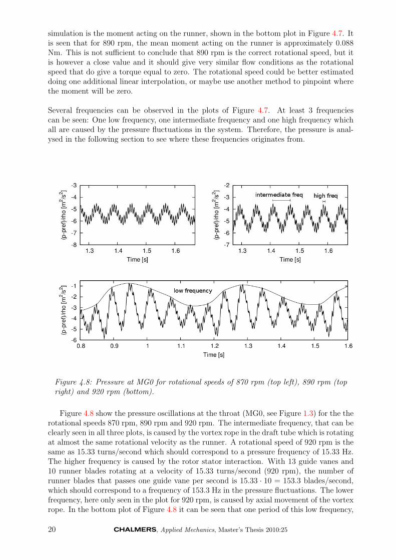
Figure 4.8: Pressure at MG0 for rotational speeds of 870 rpm (top left), 890 rpm (topright) and 920 rpm (bottom).

Figure 4.8 show the pressure oscillations at the throat (MG0, see Figure 1.3) for the therotational speeds 870 rpm, 890 rpm and 920 rpm. The intermediate frequency, that can beclearly seen in all three plots, is caused by the vortex rope in the draft tube which is rotatingat almost the same rotational velocity as the runner. A rotational speed of 920 rpm is thesame as 15.33 turns/second which should correspond to a pressure frequency of 15.33 Hz.The higher frequency is caused by the rotor stator interaction. With 13 guide vanes and10 runner blades rotating at a velocity of 15.33 turns/second (920 rpm), the number ofrunner blades that passes one guide vane per second is 15.33 · 10 = 153.3 blades/second,which should correspond to a frequency of 153.3 Hz in the pressure fluctuations. The lowerfrequency, here only seen in the plot for 920 rpm, is caused by axial movement of the vortexrope. In the bottom plot of Figure 4.8 it can be seen that one period of this low frequency,


corresponds to 5 periods of the intermediate frequency, which is the same as 5 turns ofthe runner, with each turn having a period of 1/15.33 = 0.0652 s, the period for the lowerfrequency would be 5 · 0.0652 = 0.326 s. These periods are just the time intervals thatthe pressure fluctuations should have, if it was following the motion of the runner directly,and the simulation show that they almost do. The definite frequencies of the predictedpressure fluctuations are estimated in the fourier analysis in section 4.3.

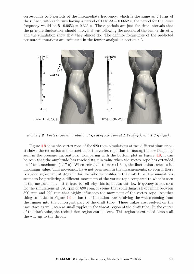
Figure 4.9: Vortex rope at a rotational speed of 920 rpm at 1.17 s(left), and 1.3 s(right).

Figure 4.9 show the vortex rope of the 920 rpmsimulations at two different time steps.It shows the retraction and extraction of the vortex rope that is causing the low frequencyseen in the pressure fluctuations. Comparing with the bottom plot in Figure 4.8, it canbe seen that the amplitude has reached its min value when the vortex rope has extendeditself to a maximum (1.17 s). When retracted to max (1.3 s), the fluctuations reaches itsmaximum value. This movement have not been seen in the measurements, so even if thereis a good agreement at 920 rpm for the velocity profiles in the draft tube, the simulationsseems to be predicting a different movement of the vortex rope compared to what is seenin the measurements. It is hard to tell why this is, but as this low frequency is not seenfor the simulations at 870 rpm or 890 rpm, it seems that something is happening between890 rpm and 920 rpm that highly influences the movement of the vortex rope. Anotherthing to notice in Figure 4.9 is that the simulations are resolving the wakes coming fromthe runner into the convergent part of the draft tube. These wakes are resolved on theisosurface as well, seen as small ripples in the throat region of the draft tube. In the centerof the draft tube, the reciculation region can be seen. This region is extended almost allthe way up to the throat.


4.3 Fourier Analysis

An analysis of the pressure fluctuations at MG0, MG1, MG2 and MG3 will be coveredin the following section. Muntean et al. [11] made a fourier analysis on Fluent andOpenFOAM simulations and compared them with measurements. The present analysisis made in Matlab using the built-in Fast Fourier Transform algorithm and the pressurevalues are taken at the transducer locations (see Figure 1.3) for the best fitted results,which was the unsteady 920 rpm simulation.(with the PISO-based solver)

4.3.1 Fourier analysis theory

Given periodic function f(t) with period T = 2L seconds, then the function f(t) can bedecomposed into a sum of components of sine and cosine functions as:

g(t) =a0

2+∞∑n=1

[ancos

(πnt

L

)+ bnsin

(πnt

T

)](4.1)

where

a0 =1

2L

∫ L

−Lf(t)dt, an =

1

L

∫ L

−Lf(t)cos

(nπt

L

)dt,

bn =1

L

∫ L

−Lf(t)sin

(nπt

L

)dt

and a0 is the mean value of f(t). an and bn are the sine and cosine mode amplitudes,respectively, for the angular frequency πn

L. This can also be expressed in the complex form:

g(t) =∞∑−∞

cneiπntL (4.2)

cn =1

2L

∫ L

−Lf(t)e−i

πntL dt, n = 0, 1, 2, 3, ...N − 1 (4.3)

A vector with N complex numbers xn = [x0, x1, ..., xN−1] can then be transformed into a fre-quency domain representation, Xk = [X0, X1, ..., XN−1] by the Discrete Fourier Transform(DFT), defined as:

Xk =N−1∑

0

xne−2πiN

kn, k = 0, 1, ..., N − 1 (4.4)

and transformed back again using its inverse (IDFT), which is defined as:

xn =1

N

N−1∑0

Xke2πiNkn, n = 0, 1, ..., N − 1 (4.5)

The DFT can be calculated using a Fast Fourier Transform algorithm.


4.3.2 Fourier algorithm in Matlab

Matlab uses a FFT algorithm called the Cooley- Tukey Fast Fourier Transform algo-rithm [7]. From the definition of eq. (4.2) it can be seen that the calculation of Xk

requires N operations that involves multiplication of two complex numbers followed by theaddition of two complex numbers. The transformation of the vector xn = [x0, x1, ..., xN−1],requires a total of N2 of these operations. If N is large , which usually is the case innumerical investigations, N2 is a lot higher, which makes the calculations hard to manage.Then, if N is not a prime, it can be decomposed into N = N1N2 and then N1 transformsof size N2 can be computed, followed by a computation of N2 transforms of size N1 and soon until the problem can be solved [8, 9]. This is what the Cooley- Tukey FFT algorithmdoes. It computes the fft and inverse fft pair for given vectors of length N by:

fft(xj) = Xk =N∑j=1

xje−2πN

(j−1)(k−1) (4.6)

ifft(Xk) = xj =1

N

N∑k=1

Xke2πN

(j−1)(k−1) (4.7)

for each number xj and each transformed number Xk.

The fourier transformed values can then be plotted in a power spectrum where the squaredabsolute value of the coefficients are plotted against the frequencies. The absolute valuesof the coefficients are the distance of the complex number to the origin, and since eachcomplex number produced by the FFT has a complex conjugate, the power and frequencyis calculated using only half of the transformed values.

power = |Xk|2 k = 1, 2, 3, ..., (N − 1)/2 (4.8)

f = nj/∆t j = 1, 2, 3, ..., (N − 1)/2 (4.9)

where nj is the j:th sample on the sampling time interval ∆t.

To compare the pressure fluctuations dimensionally, the Strohaul number can be calcu-lated:

St =f · lV

=f ·D(

4·Qπ·D2

) (4.10)

where D is the the reference length, i.e. the throat diameter = 100mm, Q is the totaldischarge of 30 l/s, and f is the fundamental frequency, in this case the vortex frequency.


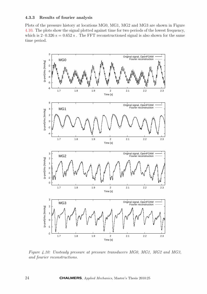
4.3.3 Results of fourier analysis

Plots of the pressure history at locations MG0, MG1, MG2 and MG3 are shown in Figure4.10. The plots show the signal plotted against time for two periods of the lowest frequency,which is 2 · 0.326 s = 0.652 s . The FFT reconstructioned signal is also shown for the sametime period.

-6

-5

-4

-3

-2

-1

0

1.7 1.8 1.9 2 2.1 2.2 2.3

(p-p

ref)

/rho

[Nm

/kg]

Time [s]

MG0Original signal, OpenFOAM

Fourier reconstruction

-4

-2

0

2

4

6

1.7 1.8 1.9 2 2.1 2.2 2.3

(p-p

ref)

/rho

[Nm

/kg]

Time [s]



-3

-2

-1

0

1

2

3

1.7 1.8 1.9 2 2.1 2.2 2.3

(p-p

ref)

/rho

[Nm

/kg]

Time [s]



-2

-1

0

1

2

3

1.7 1.8 1.9 2 2.1 2.2 2.3

(p-p

ref)

/rho

[Nm

/kg]

Time [s]

MG3 Original signal, OpenFOAMFourier reconstruction

Figure 4.10: Unsteady pressure at pressure transducers MG0, MG1, MG2 and MG3,and fourier reconstructions.


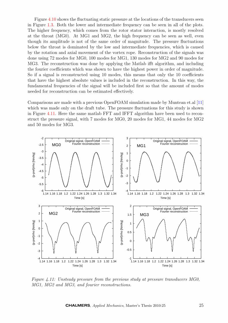
Figure 4.10 shows the fluctuating static pressure at the locations of the transducers seenin Figure 1.3. Both the lower and intermediate frequency can be seen in all of the plots.The higher frequency, which comes from the rotor stator interaction, is mostly resolvedat the throat (MG0). At MG1 and MG2, the high frequency can be seen as well, eventhough its amplitude is not of the same order of magnitude. The pressure fluctuationsbelow the throat is dominated by the low and intermediate frequencies, which is causedby the rotation and axial movement of the vortex rope. Reconstruction of the signals wasdone using 72 modes for MG0, 100 modes for MG1, 130 modes for MG2 and 90 modes forMG3. The reconstruction was done by applying the Matlab ifft algorithm, and includingthe fourier coefficients which was shown to have the highest power in order of magnitude.So if a signal is reconstructed using 10 modes, this means that only the 10 coefficientsthat have the highest absolute values is included in the reconstruction. In this way, thefundamental frequencies of the signal will be included first so that the amount of modesneeded for reconstruction can be estimated effectively.

Comparisons are made with a previous OpenFOAM simulation made by Muntean et.al [11]which was made only on the draft tube. The pressure fluctuations for this study is shownin Figure 4.11. Here the same matlab FFT and IFFT algorithm have been used to recon-struct the pressure signal, with 7 modes for MG0, 20 modes for MG1, 44 modes for MG2and 50 modes for MG3.

-6

-5.5

-5

-4.5

-4

-3.5

-3

-2.5

-2

1.14 1.16 1.18 1.2 1.22 1.24 1.26 1.28 1.3 1.32 1.34

(p-p

ref)

/rho

[Nm

/kg]

Time [s]



-4

-3

-2

-1

0

1

2

3

1.14 1.16 1.18 1.2 1.22 1.24 1.26 1.28 1.3 1.32 1.34

(p-p

ref)

/rho

[Nm

/kg]

Time [s]



-4

-3

-2

-1

0

1

2

3

1.14 1.16 1.18 1.2 1.22 1.24 1.26 1.28 1.3 1.32 1.34

(p-p

ref)

/rho

[Nm

/kg]

Time [s]



-1

-0.5

0

0.5

1

1.5

2

1.14 1.16 1.18 1.2 1.22 1.24 1.26 1.28 1.3 1.32 1.34

(p-p

ref)

/rho

[Nm

/kg]

Time [s]

MG3

Original signal, OpenFOAMFourier reconstruction

Figure 4.11: Unsteady pressure from the previous study at pressure transducers MG0,MG1, MG2 and MG3, and fourier reconstructions.


The pressure oscillations shown in Figure 4.11 has no lower or higher frequencies in-cluded in the pressure fluctuations, which is because this case was run on the draft tubeonly, without the effects of the runner included in the simulations.

0

2e+06

4e+06

6e+06

8e+06

1e+07

1.2e+07

0 20 40 60 80 100 120 140 160

Pow

er

Frequency [Hz]

MG0

OpenFOAM current studyOpenFOAM previous study

0

2e+06

4e+06

6e+06

8e+06

1e+07

1.2e+07

1.4e+07

1.6e+07

1.8e+07

0 20 40 60 80 100 120 140 160

Pow

er

Frequency [Hz]

MG1


0

2e+06

4e+06

6e+06

8e+06

1e+07

1.2e+07

0 20 40 60 80 100 120 140 160

Pow

er

Frequency [Hz]

MG2


0

2e+06

4e+06

6e+06

8e+06

1e+07

1.2e+07

0 20 40 60 80 100 120 140 160

Pow

er

Frequency [Hz]

MG3


Figure 4.12: Frequency spectra at transducer locations MG0, MG1, MG2 and MG3.

The frequency spectra in Figure 4.12 show a comparison with the previous OpenFOAMsimulation made by Muntean et.al. [11]. That study showed results that was in good agree-ment with the measurements, even though the harmonics were slightly overestimated. AtMG0, the amplitude of the 1st harmonic is almost in the same order of magnitude as theprevious study. It is seen at a frequency of 18.02 Hz, which is the same as the interme-diate frequency for 920 rpm shown in the bottom of Figure 4.8. Also, the low and highfrequencies discussed previously can be seen as the harmonics at 3.0 Hz and 153.19 Hzrespectively. At MG1, the difference in amplitude for the 1st harmonic has increased andthe present study show an amplitude about 1/3 part higher than the previous study. Theharmonics for the higher frequency harmonic at 153.19 Hz is not seen any more, and thelow frequency harmonic has been elevated. At MG2, the amplitude of the 1st harmonic isagain in good agreement with the previous study. The low frequency harmonic at 3 Hz isshown here as well with a slightly lower amplitude than at MG1. Good agreement is alsoshown at MG3 for the 1st harmonic amplitude. The vortex ropes frequency is 18.02 Hz,which corresponds to a Strohaul number of 0.480. The Strohaul number of the previousstudy was 0.427.


5 Conclusion

Meshing, steady and unsteady state simulations have been conducted on a swirl generator.The meshing have been made with ANSYS ICEM-Hexa, and the computational domainhave been aknowledged for running simulations that can be compareble with LDV data.Then steady state simulations at two different rotational speeds have been made, usingthe standard k − ε model to close the equations. The steady state simulations from bothrotational speeds are not accurately resolving the flow profiles. They serve as a goodinitial conditions for unsteady simulations, but can’t be used alone to predict the flowfeatures. Unstedy state simulations were conducted at three rotational speeds in order tofind the one corresponding to zero torque on the runner, and to compare the results fromthat rotational speed with LDV measurements. The results showed that unsteady CFDsimulations accurately predicts the flow field of the swirl generator. It was also seen, thata rotational speed of 920 rpm gives the best compareble results with LDV measurements,and that a rotational speed of 890 rpm gives almost zero torque on the runner, giventhat we don’t have any frictional forces acting on the runner. Further investigation of thepressure oscillations were conducted, which at a rotational speed of 920 rpm revealed 3distinct frequencies. One low frequency corresponding to an axial extraction/retraction ofthe vortex rope, one intermediate frequency corresponding to the rotation of the vortexrope, and one high frequency caused by the rotor stator interaction. Fourier analysis of thepressure history recorded at the wall of the draft tube showed that several new frequencieshave been introduced compared to a previous study which was made on only the drafttube.

6 Future work

Future work for this case study could be to continue investigation of the SIMPLE basedsolver and try another turbulence models such as LES or DES. This could better predictthe stagnation region seen for the meridional velocities in the draft tube. Since there hasbeen alot of time spent on finding the “correct” rotational speed for this particular setup,one idea could be to customize a solver to adjust the rotational speed in accordance tothe moment acting on the runner. This would make comparison with measurements aloteasier as it would be easier to get the definite rotational speed corresponding to zero torqueor if needed, any torque that is desired. This would also contribute to the OpenFOAMcommunity.


References

[1] Opencfd. http://www.openfoam.com.

[2] F. Avellan. Flow Investigation in a Francis Draft Tube: The FLINDT Project. InProceedings of the 20th IAHR Symposium on Hydraulic Machinery and Systems, Char-lotte, USA. Paper DES-11, 2000.

[3] M. Beaudoin and H. Jasak. Development of a Generalized Grid Interface for Tur-bomachinery simulations with OpenFOAM. In Proceedings of the OpenSource CFDInternational Conference, Berlin, Germany, 2008.

[4] A. Bosioc, S. Muntean, and R. Susan-Resiga. Numerical investigation of the jetcontrol method for swirling flow with precessing vortex rope. In Proceedings 3rdIAHR International Meeting of the Workgroup on Cavitation and Dynamic Problemsin Hydraulic Machinery and Systems, Brno, Czech Republic, October 14-16,2009.

[5] A. Bosioc, Susan-Resiga R., and S. Sebastian Muntean. Design and manufacturingof a convergent-divergent test section for swirling flow apparatus, 2008. NationalCenter for Engineering of Systems with Complex Fluids, Polytechnica University ofTimisoara, Timisoara, Romaia.

[6] A. Bosioc, C. Tanasa, S. Muntean, and R. Susan-Resiga. 2D LDV measurementsand comparison with axisymmetric flow analysis of swirling flow in a simplified drafttube. In Proceedings 3rd IAHR International Meeting of the Workgroup on Cavitationand Dynamic Problems in Hydraulic Machinery and Systems, Brno, Czech Republic,October 14-16, 2009.

[7] J. W. Cooley and J. W. Tukey. An algorithm for the machine computation of thecomplex fourier series. In Mathematics of Computation, pages Vol.19 , pp. 297–301,1965.

[8] Gerald B. Folland. Fourier Analysis and its applications. Brooks/Cole PublishingCompany, 1992.

[9] MathWorks Inc, 2010. http://www.mathworks.com/access/helpdesk/help/techdoc/ref/fft.html,april.

[10] S. Muntean, R. Susan-Resiga, A. Bosioc, A. Stuparu, A. Baya, and L.E. Anton.Mitigation of Pressure Fluctuation in a Conical Diffuser with Precessing Vortex RopeUsing Axial Jet Control Method. In Proceedings of the 24rd IAHR Symposium onHydraulic Machinery and Systems, Foz do Iguassu, Brazil, 2008.

[11] S. Muntean, R. Susan-Resiga, and H. Nilsson. 3d numerical analysis of the unsteadyturbulent swirling flow in a conical diffuser using fluent and OpenFOAM. In the 3rdIAHR International Meeting of the Workgroup on Cavitation and Dynamic Problemsin Hydraulic Machinery and Systems, Brno, Czech Republic. Brno University of Tech-nology, October 14-16,2009.

[12] H Nilsson, M. Page, M. Beaudin, B. Gschaider, and H. Jasak. The OpenFOAMTurbomachhinery Working Group, and Conclusions from the Turbomachinery Sessionof the Third OpenFOAM Workshop. In Proceedings of the 24rd IAHR Symposium onHydraulic Machinery and Systems, Foz do Iguassu, Brazil, Foz do Iguassu, October27-31, 2008.


[13] O. Petit. Investigations of Incompressible Turbomachinery Applications using Open-FOAM, 2010. Thesis of licentiate of engineering, Department of Applied Mechanics,Chalmers University of Technology, Goteborg, Sweden.

[14] R. Susan-Resiga and S. Muntean. Decelerated swirling flow in the discharge cone ofFrancis turbines. In the 4th Symposium on Fluid Machinery and Fluid Engineering,Beijing, China, November 24-27, 2008.

[15] R. Susan-Resiga, S. Muntean, and A. Bosioc. Blade design for swirling flow generator,2008. National Center for Engineering of Systems with Complex Fluids, PolytechnicaUniversity of Timisoara, Timisoara, Romaia.

[16] R. Susan-Resiga, S. Muntean, C. Tanasa, and A. Bosioc. Hydrodynamic Design andAnalysis of a Swirling Flow Generator, 2008. National Center for Engineering of Sys-tems with Complex Fluids, Polytechnica University of Timisoara, Timisoara, Romaia.

[17] R. Susan-Resiga, T.C Vu, S. Muntean, G.D Cicoan, and B. Nennemann. Jet Control ofthe Draft Tube Vortex rope in Francis Turbines at Partial Discharge. In Proceedings ofthe 23rd IAHR Symposium on Hydraulic Machinery and Systems, Yokohama, Japan.Paper F192, 2006.

[18] H.K. Versteeg and W Malalasekera. An Introduction to Computational Fluid Dynam-ics, The Finite Volmue Method. Pearson Education Limited, 2nd edition, 2007.


Documents

Numerical investigation of the flow in a swirl generator, using