Embed Size (px)
Citation preview
Thesis for the degree of doctor of philosophy
in
Thermo and Fluid Dynamics
Numerical Modelling of DieselSpray Injection, TurbulenceInteraction and Combustion
Fabian Peng Karrholm
Department of Applied Mechanics
Chalmers University of Technology
Goteborg, Sweden, 2008
Numerical Modelling of Diesel Spray Injection, Turbulence
Interaction and Combustion
Fabian Peng Karrholm
The image on the cover of the thesis is an illustrative image of a lagrangianspray, evaporation has been turned off to improve the visual experience.
c©Fabian Peng Karrholm, 2008
Doktorsavhandling vid Chalmers Tekniska Hogskola
First editionISBN: 978-91-7385-173-2ISSN: 0346-718XNy Serie: 2854
Department of Applied MechanicsChalmers University of TechnologySE-412 96 GoteborgSweden Telephone +46 31 772 10 00
Printed at Chalmers ReproserviceGoteborg, Sweden 2008
I guess this is my dissertationHomie this ... is basic, Welcome to Graduation
Good morning,Good morning
On this day, we become legendary- Kanye West

iii
AbstractThis thesis covers two main topics. The first is numerical modelling ofcavitating diesel injector flows, focusing on describing such flows using asingle-phase cavitation model based on a barotropic equation of state togetherwith a homogenous equilibrium assumption. The second topic isEuler-Lagrangian simulations of diesel sprays, focusing on attempts to reducethe high grid/timestep dependencies in numerical simulations of diesel sprays.In addition, the ability of two CFD codes to predict flame lift-off length andignition delay time, and the advection scheme’s influence on fuel distributions,are considered.
A long-term goal was to develop a new atomization model based on calculatedflows in injector nozzles, which did not have the drawback of requiring eithernon-physical parameters or information derived from specific experiments. Tovalidate the cavitation simulations, comparisons were made with experimentaldata obtained at AVL. The experimental data (which are practically 2D)provide information on velocity profiles and pressure contours. These datawere used to validate the code. However, since the code is not stable fordiesel-type pressures, no atomization model was developed.
The main part of the thesis describes how diesel sprays were simulated usingthe discrete droplet model (DDM), in which the liquid is described byLagrangian coordinates and the vapour by an Eulerian approach. Thesimulations have been used to investigate how the k-ε family of turbulencemodels influence spray behaviour, and a simple but efficient way to reduce thedependency of the mesh resolution, by limiting the turbulence length scale inthe liquid core region, is proposed. This constraint is shown to have a positiveeffect on the spray behaviour, and to reduce both grid and timestepdependencies.
In addition, the ignition delay time and flame lift-off lengths have beeninvestigated, since these two properties are believed to be important foremissions formation. The simulations used a complex chemical mechanisminvolving 83 species and 338 reactions. The effects of the numerical scheme,the turbulence model and physical parameters (like ambient temperature andoxygen content) on these variables have also been investigated.
Keywords: Spray, Computational Fluid Dynamics, Diesel, Turbulence Model,Cavitation, Atomization, Flame, Lift-off, Ignition Delay, Numerical Scheme,TVD, Combustion

iv
Acknowledgements
I thank Niklas Nordin for his supervision, help and guidance in OpenFOAM,especially during the first years of my phd studies. I am also in debt to FengTao, thank you for your enthusiasm, discussions, suggestions, encouragementand help during the latter part. I also owe a great deal to Rasmus Hemph forthe many discussions on the mysteries of OpenFOAM, CFD and autolyse.Thanks also goes out to Ingemar Denbratt for his enthusiasm and support. Ithank Alf-Hugo Magnusson for providing experimental data for paper 1. I alsowant to thank everyone else at the department, new and old. I have reallyappreciated the lunch & coffee breaks as well as discussions on morework-related matters.
I also wish to thank some people abroad, who have helped me during my timeat Chalmers. Dr. Tommaso Lucchini who I am proud to have shared officewith, and who showed me the path to self-learning in OpenFOAM. Dr HrvojeJasak for helping me with the appendix on Rhie-Chow, the work you do forOpenFOAM is priceless. Henry Weller for his assistance on the second paper,and for answering to so many of my questions on cavitation and itsimplementation in the code. I thank Dr. Ernst Winklhofer for sharing hisexperiments on cavitating nozzles.
I thank the Combustion Engine Research Center (CERC) for providingfinancial support for this work on Diesel Sprays.
Last, I want to thank my family, Cecilia PK, Edwin P and Alicia K. Afterall,you are the ones who makes everything worthwhile. I also thank myself forhanging in there, and accomplishing this.
v

vi
Nomenclature
Roman Symbols
b Relaxation coefficientc Molar Concentration mol/m3
cl Liquid specific heat at constant volume J/kgKcp,v Fluid specific heat at constant volume J/kgKC1,C2,C3,Cµ Turbulence model constantsCD Drag coefficientCd Discharge coefficient of nozzleCe Constant of the D2-lawCo Courant numberd Droplet diameter mD Droplet Diameter mD Mass Diffusion Coefficient m2/sEa Arrhenius Activation Energy J/molF Force on particle kgm/s2
Fs Spray momentum source term kgm/s2
f Coefficient in RNG turbulence modelfheat Correction factor for heat exchange due to mass transferg Gravitation acceleration vector m/s2
hv Enthalpy of vapour J/kgk Kinetic energy of turbulent fluctuations m2/s2
kj Arrhenius constant of reaction jl∞ Relaxation length scale mlt Length scale of turbulent fluctuations mLsgs Maximum user-set length scale mm Mass kgn Parameter for Rosin-Rammler distributionn Face NormalNr Number of reactionsNs Number of speciesNu Nusselt numberOh Ohnesorge numberp0 Pressure at outlet in previous time step Pap∞ Desired outlet pressure Pap Pressure Pa
vii
viii
p Momentum kgm/sRRNG Coefficient in the RNG k-ε turbulence modelR Universal Gas Constant J/KmolRRi Reaction Rate of species iRe Reynolds number of fluidS Strain 1/sSfa Help variableSc Schmidt numberSh Sherwood numberT Temperature of fluid Kt Time sTa Taylor numberu,U Velocity m/sw Outgoing pressure wave velocity m/sWe Weber numberXi Volume fraction of scalar iXv,s Mass fraction of fuel vapour at droplet surfaceXv,∞ Mass fraction of fuel vapour far awayYi Mass fraction of scalar i
Greek Symbols
α Volume fraction of fluidαk,αε Turbulence model constantβ Volume fraction of fluidβmax Maximum spray cone angleγ Vapour (cavitated liquid) fractionδ Cell-face distance coefficient m∆t Time-step sε Dissipation rate m2/s3
κc Thermal Conductivity W/mKλ Limiter function for interfaceCompression-schemeΛ Wavelength of fastest growing wave mµ Laminar viscosity kg/msµT Turbulent viscosity kg/msν Kinematic viscosity m2/sρ Density kg/m3
ρs Spray mass source term kg/m3sτe Relaxation time of evaporation sτu Momentum relaxation time sφ Volume flow across cell face m3/sψ Compressibility s2/m2
Ω Growth rate of fastest growing wave m/s2
Contents
1 Introduction 1
1.1 Background & Motivation . . . . . . . . . . . . . . . . . . . . . . 1
1.2 Simple Description of the Computational Approach . . . . . . . . 4
1.3 Implementation and Code . . . . . . . . . . . . . . . . . . . . . . 5
1.4 Outline of the Thesis . . . . . . . . . . . . . . . . . . . . . . . . . 6
2 Nozzle Flow 9
2.1 Previous Works in the Field . . . . . . . . . . . . . . . . . . . . . 10
2.2 A Code for Cavitating Diesel Injector Flow into Air . . . . . . . 11
2.3 Boundary Conditions for Pressure . . . . . . . . . . . . . . . . . 15
2.3.1 Inlet . . . . . . . . . . . . . . . . . . . . . . . . . . . . . . 15
2.3.2 Outlet . . . . . . . . . . . . . . . . . . . . . . . . . . . . . 15
2.4 A Code for Cavitating Single-Phase Flow . . . . . . . . . . . . . 16
2.4.1 Development of Injection Model . . . . . . . . . . . . . . 19
3 Spray Modelling 21
3.1 The Gas Phase . . . . . . . . . . . . . . . . . . . . . . . . . . . . 22
3.1.1 Basic Equations . . . . . . . . . . . . . . . . . . . . . . . 22
3.1.2 Turbulence Modelling . . . . . . . . . . . . . . . . . . . . 23
3.1.3 Turbulence/Spray Interaction . . . . . . . . . . . . . . . . 24
3.1.4 Chemistry . . . . . . . . . . . . . . . . . . . . . . . . . . . 27
3.2 Spray Sub-Models . . . . . . . . . . . . . . . . . . . . . . . . . . 30
3.2.1 Spray Motion Equation . . . . . . . . . . . . . . . . . . . 30
ix
x CONTENTS
3.2.2 Parcel Tracking . . . . . . . . . . . . . . . . . . . . . . . . 31
3.2.3 Injection Model . . . . . . . . . . . . . . . . . . . . . . . . 32
3.2.4 Drag Model . . . . . . . . . . . . . . . . . . . . . . . . . . 32
3.2.5 Breakup Model . . . . . . . . . . . . . . . . . . . . . . . . 33
3.2.6 Evaporation Model . . . . . . . . . . . . . . . . . . . . . . 34
3.2.7 Heat Transfer . . . . . . . . . . . . . . . . . . . . . . . . . 36
3.2.8 Particle Collisions . . . . . . . . . . . . . . . . . . . . . . 37
4 Results & Discussion 39
4.1 Simulations of a Diesel Flow in a Cavitating Model Nozzle . . . . 39
4.2 Injector Simulation Results . . . . . . . . . . . . . . . . . . . . . 43
4.2.1 Impact of Injection Model . . . . . . . . . . . . . . . . . . 44
4.3 Spray Results without Chemistry . . . . . . . . . . . . . . . . . . 46
4.3.1 Grid Dependency . . . . . . . . . . . . . . . . . . . . . . . 46
4.3.2 Time Step Dependency . . . . . . . . . . . . . . . . . . . 48
4.3.3 Comparison to Experimental Data . . . . . . . . . . . . . 50
4.4 Influence of Numerical Scheme . . . . . . . . . . . . . . . . . . . 51
4.5 Fuel Sprays with Chemistry . . . . . . . . . . . . . . . . . . . . . 53
4.5.1 Combustion Predictions Using Other Schemes . . . . . . . 57
4.6 Comment on the PaSR Model . . . . . . . . . . . . . . . . . . . . 59
5 Conclusions 61
6 Future Work 63
6.1 Outlook . . . . . . . . . . . . . . . . . . . . . . . . . . . . . . . . 64
7 Summary of Papers 67
A Implementation in OpenFOAM 71
A.1 Rhie-Chow Interpolation in OpenFOAM . . . . . . . . . . . . . . 71
A.2 Formulating the Momentum Equation Matrix in OpenFOAM . . 76
B Variable Definitions and Dimensionless Numbers 79
Chapter 1
Introduction
1.1 Background & Motivation
Today, cars and heavy duty vehicles are considered to be major sources ofenvironmental pollution. However, when the first automobiles appeared in thestreets of New York and London they were considered to be solutions toanother problem: horse manure. According to a rough estimate published inAppleton’s magazine in 1908, 20 000 New Yorkers died each year from“maladies that fly in the dust, created mainly by horse manure”. Details of thedata used to obtain the estimate are unknown, but there is no doubt thathorses, and the resulting manure, constituted a major environmentalproblem[1]. In the late 19th century, Nikolaus Otto in 1876, and later RudolfDiesel in 1897 patented their prime mover inventions. Horse manure became aproblem of the past. However, now, over 100 years later, we are facing a newenvironmental threat, and this time our former saviours have become ourproblem.
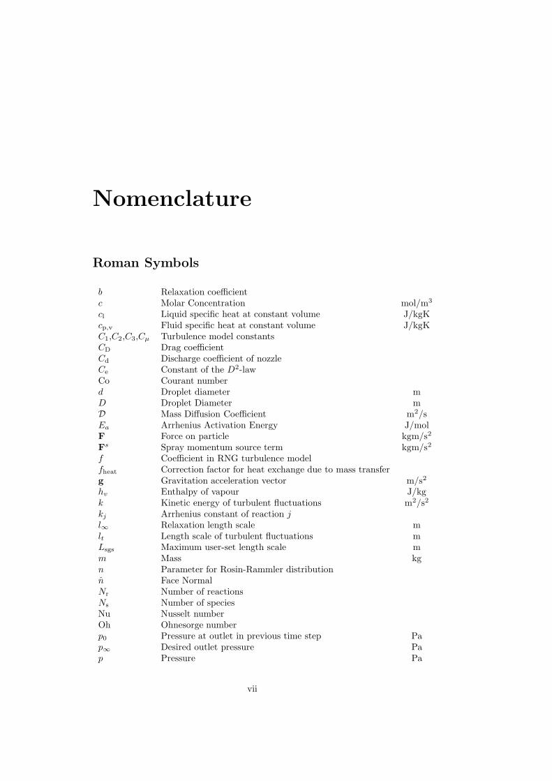
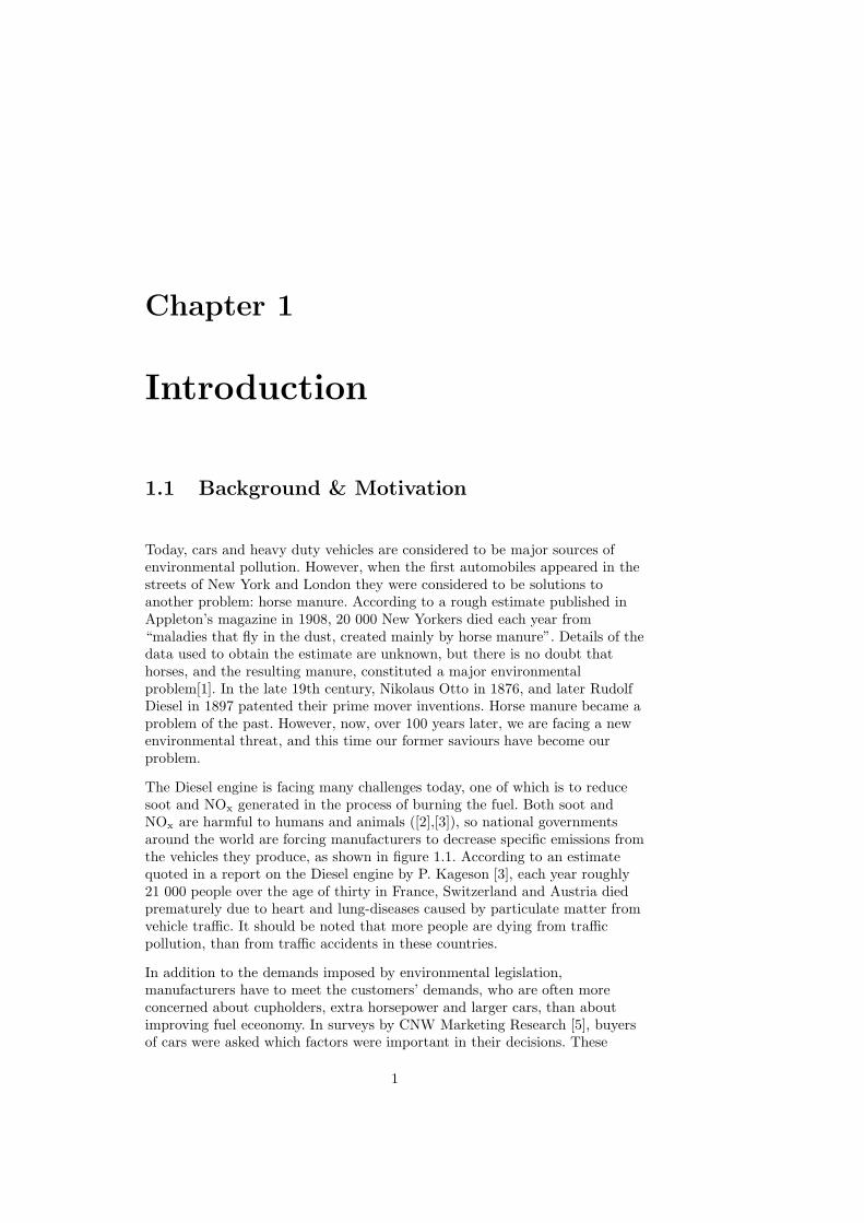
The Diesel engine is facing many challenges today, one of which is to reducesoot and NOx generated in the process of burning the fuel. Both soot andNOx are harmful to humans and animals ([2],[3]), so national governmentsaround the world are forcing manufacturers to decrease specific emissions fromthe vehicles they produce, as shown in figure 1.1. According to an estimatequoted in a report on the Diesel engine by P. Kageson [3], each year roughly21 000 people over the age of thirty in France, Switzerland and Austria diedprematurely due to heart and lung-diseases caused by particulate matter fromvehicle traffic. It should be noted that more people are dying from trafficpollution, than from traffic accidents in these countries.
In addition to the demands imposed by environmental legislation,manufacturers have to meet the customers’ demands, who are often moreconcerned about cupholders, extra horsepower and larger cars, than aboutimproving fuel eceonomy. In surveys by CNW Marketing Research [5], buyersof cars were asked which factors were important in their decisions. These
1
2 CHAPTER 1. INTRODUCTION
1990 1995 2000 2005 20100
0.5
1
1.5
2
2.5
3
year
g/km
NOx
PMHC+NO
x
CO
Figure 1.1: Changes in legal limits for emissions from automobiles within theEU, 1992-2008 [4].
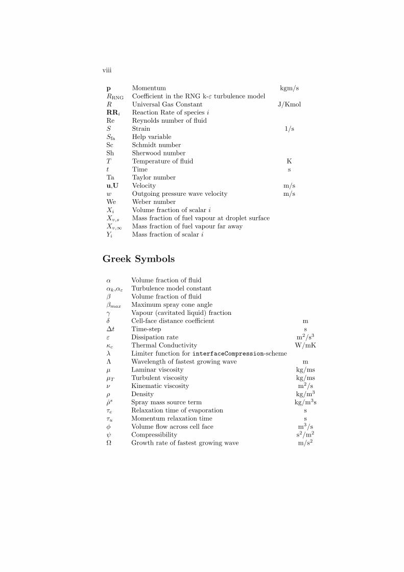
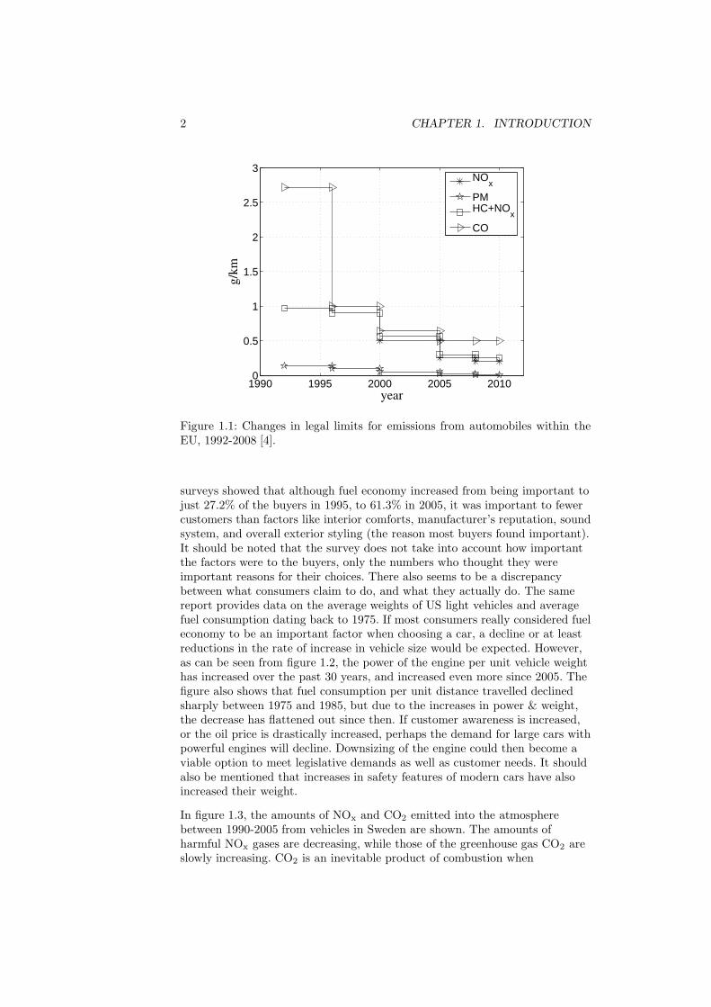
surveys showed that although fuel economy increased from being important tojust 27.2% of the buyers in 1995, to 61.3% in 2005, it was important to fewercustomers than factors like interior comforts, manufacturer’s reputation, soundsystem, and overall exterior styling (the reason most buyers found important).It should be noted that the survey does not take into account how importantthe factors were to the buyers, only the numbers who thought they wereimportant reasons for their choices. There also seems to be a discrepancybetween what consumers claim to do, and what they actually do. The samereport provides data on the average weights of US light vehicles and averagefuel consumption dating back to 1975. If most consumers really considered fueleconomy to be an important factor when choosing a car, a decline or at leastreductions in the rate of increase in vehicle size would be expected. However,as can be seen from figure 1.2, the power of the engine per unit vehicle weighthas increased over the past 30 years, and increased even more since 2005. Thefigure also shows that fuel consumption per unit distance travelled declinedsharply between 1975 and 1985, but due to the increases in power & weight,the decrease has flattened out since then. If customer awareness is increased,or the oil price is drastically increased, perhaps the demand for large cars withpowerful engines will decline. Downsizing of the engine could then become aviable option to meet legislative demands as well as customer needs. It shouldalso be mentioned that increases in safety features of modern cars have alsoincreased their weight.
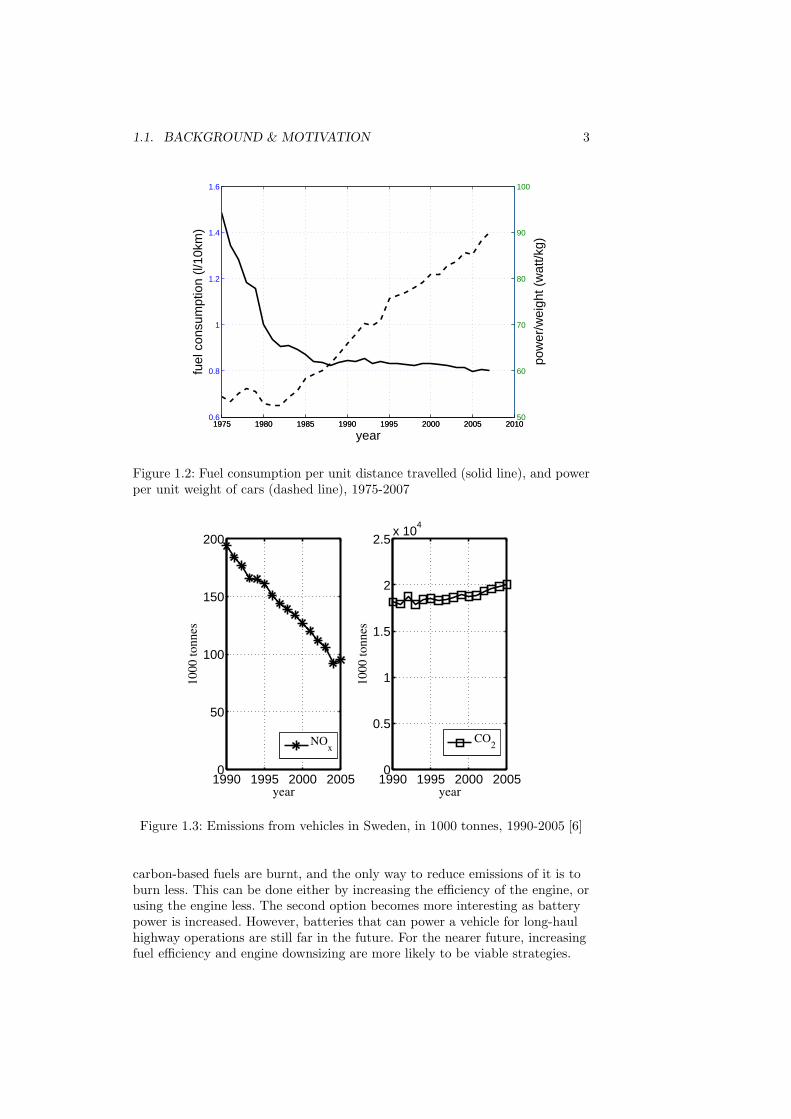
In figure 1.3, the amounts of NOx and CO2 emitted into the atmospherebetween 1990-2005 from vehicles in Sweden are shown. The amounts ofharmful NOx gases are decreasing, while those of the greenhouse gas CO2 areslowly increasing. CO2 is an inevitable product of combustion when
1.1. BACKGROUND & MOTIVATION 3
1975 1980 1985 1990 1995 2000 2005 20100.6
0.8
1
1.2
1.4
1.6
year
fuel
con
sum
ptio
n (l/
10km
)
1975 1980 1985 1990 1995 2000 2005 201050
60
70
80
90
100
pow
er/w
eigh
t (w
att/k
g)
Figure 1.2: Fuel consumption per unit distance travelled (solid line), and powerper unit weight of cars (dashed line), 1975-2007
1990 1995 2000 20050
50
100
150
200
year
1000
tonn
es
NOx
1990 1995 2000 20050
0.5
1
1.5
2
2.5x 10
4
year
1000
tonn
es
CO2
Figure 1.3: Emissions from vehicles in Sweden, in 1000 tonnes, 1990-2005 [6]
carbon-based fuels are burnt, and the only way to reduce emissions of it is toburn less. This can be done either by increasing the efficiency of the engine, orusing the engine less. The second option becomes more interesting as batterypower is increased. However, batteries that can power a vehicle for long-haulhighway operations are still far in the future. For the nearer future, increasingfuel efficiency and engine downsizing are more likely to be viable strategies.
4 CHAPTER 1. INTRODUCTION
There are two branches of research concerning the optimization of enginedesign and operators: one involving experiments with physical engines, and theother involving attempts to model engines numerically. A symbolicrelationship between the two approaches is usually employed, since neither ofthem can capture all the relevant details. The experimenter does not knowexactly what happens inside the engine, and the modeller cannot be certainthe events predicted by the model are correct without experimentalverification. However, with a verified model, a reasonable description of theprocesses taking place can be obtained. In addition, the modeller has all thedata available from them. Another advantage of modelling is that it allowsconceptual engines and combustion modes to be explored long beforeprototypes are made. Simulations can also be useful for parameter studies,where they provide a cheaper alternative than large-scale engine studies.
1.2 Simple Description of the Computational
Approach
CFD is an abbreviation of Computational Fluid Dynamics, and refers tosolving a finite approximation of the Navier-Stokes equations numerically. Thespatial domain of interest, for example the cylinder of an engine, the shape ofa car, or the inside of a diesel injector, is divided into several small cells orcontrol volumes. The sum of the control volumes, called a mesh, provides afinite approximation of the spatial domain. Solving conservation equationsusing such a mesh is called an Eulerian approach, meaning that each positionin space has a numerical representation. For instance, a thermometer thatmeasures the outdoor temperature at the same spot every day provides anexample of an Eulerian description of temperature. Another way to describereality is to follow a particle, and compute its state vector, including variablessuch as its position over time, conserving momentum and energy. Thisapproach, known as Lagrangian, is particularly appropriate when all forcesacting on an object are known. For example, the path of a rocket can beconveniently described in Lagrangian coordinates, as all forces acting on therocket moves with it.
A combination of these two representations is often used in Diesel spraysimulations. The air in the combustion chamber is described using an Eulerianframework, and the liquid spray is discretised into computational ’parcels’,each of which is described by Lagrangian coordinates. That is, we inject partof the spray, and track its position in time. The parcels may consist of anynumber of droplets, each of which is considered identical, depending on valuesset by the user. Each of these parcels is subject to the same processes as a realdiesel spray, including (inter alia): atomization, break-up, collision,evaporation, heat transfer and turbulence. The processes mentioned, such asheat transfer, occur as integral operations over the particle’s entire surface,but resolution of particle surfaces is computationally prohibitive. Therefore, a’point particle’ approximation is typically made, which requires a largenumber of sub-models to empirically account for integral fluxes over the
1.3. IMPLEMENTATION AND CODE 5
particle surfaces. Further sub-models, requiring still more empiricism, areneeded to model physical processes such as atomization. Unfortunately, mostof the sub-models available today are quite unreliable, and depend on the userto supply constants that have limited physical interpretability. These constantscan often differ widely between authors, and publications, depending on thetype of spray behaviour being considered. A typical example is the breakupconstant in the KelvinHelmholz-RayleighTaylor model ([7],[8],[9]), which canvary over an order of magnitude.
1.3 Implementation and Code
The code used in the work this thesis is based upon was OpenFOAM ([10]&[11]); an open-source code available at www.openfoam.com. It is anobject-oriented code written in C++, which makes it reasonablystraightforward to implement new models and fit them into the whole codestructure. OpenFOAM is being continously developed; when I started mydoctoral studies I used Nabla FOAM 1.2, followed by OpenFOAM 1.0 up untilthe recent 1.4.1 (the latest, 1.5, release has not been used). The code nowincludes polyhedral mesh support, making it possible to create meshes usingany form of cells, as long as the quality of the resulting mesh is high.Lagrangian parcels are tracked by face-to-face tracking, thus no parcels arelost when moving between cells as in Kiva-3V. Further, models areimplemented to be run-time-selectable, which makes it very easy for the userto switch between turbulence models, spray sub-models, numerical schemesetc. OpenFOAM has many other advantages1, but one of the most importantis the complete parallelization of the code. All solvers written in OpenFOAMcan easily be run in parallel, since the code is parallelized at such afundamental level, removing the need (in most cases) for the user to considermultiple processor simulations.
OpenFOAM code was chosen both because of the high scope it offers fordeveloping new models, and the demands it places on the user. It is moredifficult to not know what you are doing in OpenFOAM, than in other codes.One could argue that access to source code, and knowledge of what one isdoing, can easily be achieved by using an in-house code. While this is true, Ibelieve that research should generally be done in a community in whichexchange of information is the norm, and an important contributor toprogress. The ability to share codes and ideas developed in the sameframework is one of OpenFOAM’s most important strengths.
1One of the most recent additions is an automatic mesh generator.
6 CHAPTER 1. INTRODUCTION
1.4 Outline of the Thesis
The Introduction chapter presents basic information about sprays, andmotivation for the work. The idea is that this chapter should beunderstandable to people without a degree in engineering. Subsequentchapters assume a knowledge of basic university level math and physics. In thefollowing chapters, the project is described in the same order that the fueltravels, starting with the nozzle flow, and then on to the spray calculations,turbulence interactions and combustion. Some parts of the modelling havebeen described twice (in both papers and the thesis), but such repetition hasbeen kept to a minimum. Where it is included, it is included for continuity, orbecause the description in the article was too concise due to size limitations.
The goals of the work have been to improve existing models for diesel spraysimulations, and to develop better models. Spray modelling today is at a stagewhere there is a heavy reliance on experimental data for validation. Oneexample is the dependency on the computation grid. The errors in spraysimulations do not follow the common CFD rule of decreasing as the numberof cells is increased[12]. Instead, the discretization error has a minimum for aspecific grid size, due to the relationship between the liquid (Lagrangianparcels) and the gas (Eulerian cells). The minimum has to be found on acase-to-case basis, and the results compared to experimental data to determinewhich grid is most suitable. Therefore, spray simulations are more sensitive tothe grid than other CFD simulations, since an increase in the number of cellscan either increase or decrease the quality of the simulation. If some of thisgrid dependency could be reduced, it would be of great value to the numericalcommunity.
Euler-Lagrangian spray simulations uses sub-models to describe the processesthat affect the injected liquid. One of the models that has been focused on inthis work is the injection and atomization model. The model is used to obtaininitial droplet size and velocity parameters, thus it has a major influence onthe initial breakup of the spray. Atomization refers to the primary breakup ofthe liquid core of the spray, and it is separated from secondary breakup, whichdescribes how liquid droplets are split into smaller droplets. An atomizationmodel can be used to describe how the droplets break up initially, or simplyswitch off breakup within a certain distance from the injector. The mostcommon way to inject droplets in Euler-Lagrangian sprays is to use a sizedistribution and randomly inject droplets from the injector in directionswithin the prescribed cone angle. A better injection model taking cavitation,turbulence and the flow in the nozzle into account that is only dependent onphysical parameters could increase the quality of the simulations. Therefore, agoal of this project was to develop such a model, which does not prescribe aninjection angle and droplet distribution, but calculates it from set variablessuch as the injection pressure, fuel density, length and width of the nozzle etc.
A very important parameter for diesel simulations is the flame lift-off length,which is believed to have a strong effects on the emissions generated duringcombustion, since increasing it will cause the flame to have a more premixedcharacter and consequently yield lower emissions of NOx and particulate
1.4. OUTLINE OF THE THESIS 7
matter. The lift-off length phenomenon is quite complex, and requires awell-developed spray model to even appear. If inappropriate schemes,sub-models and combustion models are employed the flame will spread all theway to the nozzle and no lift-off length will be observed. It is also closely linkedto the ignition delay time, which is very important for engine simulations sincefull control over the ignition is highly desirable. Attempts were also made tobench-mark OpenFOAM’s performance in terms of simulating thesephenomena, and compare it to that of the commonly used KIVA-3V code.
The last issue addressed during the work underlying this thesis were the effectsof numerical schemes and initial turbulent viscosity on the solution. It wasdiscovered quite early on (during the studies described in Paper 1) that thechosen scheme and initial parameters have a large influence over the resultingspray. Part of the reason why this was studied is the wide variety of schemesavailable in OpenFOAM, in which it is very easy to switch between differenttypes.

8 CHAPTER 1. INTRODUCTION
Chapter 2
Nozzle Flow
In both Diesel engines and direct injection spark ignition engines fuel isinjected into the combustion chamber by high pressure. Ideally, it should thenatomize, form small droplets, and eventually completely evaporate, yielding amixture that is easily combustible without forming either soot or NOx. In aspark ignition engines it is also important to position the fuel cloud close tothe spark plug to promote good combustion. The atomization, i.e. theformation of the initial droplets and their breakup, is mainly governed by theflow in the nozzle which ejects the spray ([13]). It is therefore important tostudy the flow inside the nozzle, to find out how it is linked to the spray in thecylinder. Furthermore, cavitation is believed to have a strong influence on theflow inside the nozzle, so it is also important to consider these effects.
Cavitation can occur when fluid of high velocity passes through a contractionlike a nozzle. A pocket of low pressure is formed in the wake of thecontraction’s edge, and if the pressure in this wake is sufficiently low, i.e.below the saturation pressure, the liquid will cavitate. The size of thecavitation bubbles will depend on several factors, including injection pressure,geometry, smoothness of the interior of the nozzle, and the properties of thefluid. For example, if the fluid is pushed through the nozzle sufficiently slow,no cavitation will occur and ordinary pipe flow will be observed.
Cavitation introduces vapour bubbles into the flow and increases themaximum velocity in the centre. The velocity is increased for two reasonswhen the fluid is cavitating. Firstly, if there is vapour along the walls theliquid will not have a no-slip condition boundary since the vapour will not bestationary, thus allowing the velocity of the liquid to increase (which isessential when there is a high pressure drop over the nozzle). Secondly, whenthe fluid is cavitating the liquid can not fill the entire channel. Furthermore,since the vapor bubbles formed in the nozzle are mixed with the liquid, whenthey reach the combustion chamber the ligaments and droplets formed arealready partly evaporated through cavitation. The remaining liquid willevaporate faster, and the entire atomization process will be accelerated.
9
10 CHAPTER 2. NOZZLE FLOW
2.1 Previous Works in the Field
The flow inside a diesel nozzle has been studied by many researchers, bothexperimentally ([14],[15],[16],[17]), and numerically ([17],[18],[19],[20]). Theresults from [15] by Winklhofer et al have been used in this work to validatethe single-phase cavitation model. They have been used previously in [21]using a Rayleigh Bubble Growth model [22]. In some studies nozzle flowcalculations have been coupled to Lagrangian spray simulations ([23]) on acase-to-case basis, but few authors have performed nozzle simulations withintention to create a new atomization model for Euler-Lagrangian diesel spraysimulations covering a comprehensive range of initial conditions. An exceptionis Ning [24], who developed a new atomization model for the Euler-LagrangianSpray and Atomization (ELSA) approach. ELSA is a mixture of modellingapproaches in which a full Eulerian description is used for the near-nozzle flowwhere the spray is dense, but if the liquid volume fraction falls below auser-set value, it is transformed into a Lagrangian parcel.
An additional complication when modelling cavitation that most studies haveneglected (one exception is [25]) is the effect of cavitation in multi-holeinjectors. As reported by Nouri et al in [26], strings of cavitation can occurbetween different nozzle holes in multi-hole injectors and the strings reducethe effective hole flow area, which in turn increases the flow velocity.
Cavitation is usually modelled using either Rayleigh bubble growth dynamicstheory in conjunction with a volume of fluid method ([17],[22],[27]) or, theHomogenous Equilibrium Model (HEM,[20],[28]), which assumes that thecavitated mixture is perfectly mixed and the amount of cavitation can bedescribed by a vapour mass fraction between 0 and 1. In both approaches anassumption about isentropic nozzle flow is usually included, and the HEMapproach needs an equation of state relating pressure and density to calculatethe growth of cavitation. The Rayleigh bubble growth approach solves atransport equation for the liquid-gas interface, with a source term to modelcavitation, calculated from a simplified Rayleigh equation. There is also athird approach, based on Gibbs free energy [29], which is very rarely used.
Previous works in the field have modelled cavitating liquid, but not theambient air in the combustion chamber. This is often an essentialsimplification due to the difficulty of resolving three phases while maintainingreasonable computational times. As part of this project, OpenCFD Ltd. wascontracted to develop a code handling liquid, cavitating liquid and ambientair. The resulting code has not been validated within this project, due toproblems in its handling of diesel fuel flows. However, it is possible to use it tosimulate water injections, although the simulation time extends over severalweeks. This code was originally described in [30], but since the citedpublication has limited availability it will also be described here. A simplercode (presented in the following section) for a cavitating fluid was alsodeveloped as part of the project.
2.2. A CODE FOR CAVITATING DIESEL INJECTOR FLOW INTO AIR11
2.2 A Code for Cavitating Diesel Injector Flowinto Air
The purpose of this code is to simulate cavitating diesel fuel injected into achamber filled with air. Even though the code can have other uses, simulatingdiesel injections was its original purpose. In this text, gas refers to the ambientgas which the liquid is injected into, and vapour to liquid that undergoescavitation. To simulate the liquid-gas interface, the Volume of Fluid (VOF)method is used, in which the liquid phase is allowed to cavitate and the gasphase can be compressed due to pressure shocks. The equations that need tobe solved are, as usual, the momentum equation and the continuity equation,presented below:
∂ρU
∂t+ ((U · ∇)ρU) −∇ · (µ∇U) = −∇p (2.1)
with
µ = α(γµα,v + (1 − γ)µα,l) + βµβ + µsgs (2.2)
where α and β are the fuel and air volume fractions, respectively. Therelationship between these two is:
α+ β = 1 (2.3)
In equation 2.2, the vapour fraction is described by γ, indicating theproportion of the cells that are cavitated.
γ =ρα,lv − ρα,lSat
ρα,vSat − ρα,lSat(2.4)
The code uses a Large Eddy Simulation (LES) model, which is apparent inequation 2.2 in the µsgs-term. LES is believed to be necessary in order toresolve the liquid turbulence interaction with the low turbulence in the gasphase.
In addition to the momentum equation there is the continuity equation foreach phase:
∂αρα∂t
+ ∇ · (ρααU) = 0 (2.5)
∂βρβ∂t
+ ∇ · (ρββU) = 0 (2.6)
where
12 CHAPTER 2. NOZZLE FLOW
ρ = αρα + βρβ (2.7)
and thus equations 2.5 & 2.6 can be combined to form
∂ρ
∂t+ ∇ · (ρU) = 0 (2.8)
Since the code is intended to account for compressibility an equation of state(EOS) relating pressure and density is needed. There was a more detailedrationale for the EOS used in the studies presented in Paper 2, but that codedoes not use VOF and thus only one EOS is needed. For modelling dieselinjection into air two equations of state are needed, one for liquid and one forthe gas. The main reason for selecting the chosen EOS (for the liquid) is thatit obeys the liquid and vapour EOS in the limit cases of pure liquid and purevapour, and some form of mixture for the intermediate states. The gas EOS issimpler, since it is assumed to not undergo any phase-changes:
ρliq,vap = (1 − γ) ρ0l + (γψv + (1 − γ)ψl) p
sat + ψ(γ)(p− psat
)(2.9)
ρair = ψgp (2.10)
Where ψv and ψl refers to the vapour and liquid compressibility, respectively.For reference, it is related to the speed of sound by:
a =1√ψ
(2.11)
The constant ρ0l is defined as
ρ0l = ρl,sat − psatψl (2.12)
When the code is executed the model for ψ is chosen at runtime. Three modelshave been implemented: the Wallis equation [31]:
ψWallis = (γρv,Sat + (1 − γ)ρl,Sat)
(
γψv
ρv,Sat+ (1 − γ)
ψl
ρl,Sat
)
(2.13)
the Chung equation [32]:
sfa =
ρv,Sat
ψv
(1 − γ)ρv,Sat
ψv+ γ
ρl,Sat
ψl
(2.14)
ψChung =
((1− γ√ψv
+γsfa√ψl
) √ψvψl
sfa
)2
(2.15)
2.2. A CODE FOR CAVITATING DIESEL INJECTOR FLOW INTO AIR13
and a linear model:
ψlinear = γψv + (1 − γ)ψl (2.16)
The linear model was the one chosen for this work, since it is then consistentwith the VOF-method, where viscosity and mass fraction are also described bylinear equations. The Wallis model represents the lower speed of sound(compressibility) in a bubbly mixture in a more physical way, but it was foundto be quite unstable when used for high speed flows. When a linearcompressibility model is used, the EOS for the liquid can be reduced to:
ρliq,vap = ρl,sat + ψp (2.17)
We can now return to equations 2.5 and 2.6, and form equations that are moresuitable for solving for the phase fraction and densities. We can begin byseparating the two equations into two components: one representingincompressible flow, and the other the compressibility effects.
∂α
∂t+ ∇ · (αU) = − α
ρα
DραDt
(2.18)
∂β
∂t+ ∇ · (βU) = − β
ρβ
DρβDt
(2.19)
These two equations could be solved for α and β respectively with the righthand side as the compressible “source”. However, when these equations arediscretized, they will not be mass-conservative, since there is no couplingbetween α and β when they are solved. The way the phase fraction variablesare calculated will be described later. If the two equations above are combinedwith 2.3 an equation for the divergence of U is formed:
∇ ·U = − α
ρα
DραDt
− β
ρβ
DρβDt
(2.20)
This equation is used with the discretized momentum equation and theequation of state (equations 2.9 & 2.10, respectively) to form the equation forpressure. An example of how this is done for a simpler code (icoFoam) can befound in Appendix A.1.
Equations for U and p have now been derived, and by using the equation ofstate, the density can be found. However, we also need an equation to convectthe density for the momentum equation, which has already been defined in 2.5& 2.6. They can be re-arranged into:
14 CHAPTER 2. NOZZLE FLOW
∂ρα∂t
+ ∇ · (ραU) = ραβ
(1
ρα
DραDt
− 1
ρβ
DρβDt
)
(2.21)
∂ρβ∂t
+ ∇ · (ρβU) = ρβα
(1
ρβ
DρβDt
− 1
ρα
DραDt
)
(2.22)
These equations are used to convect ρ and illustrate that if the materialderivatives of either density is larger than the other, it will result in anegative/positive right hand side. Further, the phase densities will remainsingle-phase if either α or β is zero. The terms within the parenthesis on theright hand side are treated explicitly, when the equations are solved for ρα andρβ .
The last two variables that need to be solved for are the phase-fractions. Theequation to be solved can be derived from 2.18 & 2.19, where the convectionterm is evaluated and 2.20 is used to eliminate the divergence term. Thisresults in:
∂α
∂t+ U · ∇α = −αβ
(1
ρα
DραDt
− 1
ρβ
DρβDt
)
(2.23)
∂β
∂t+ U · ∇β = −αβ
(1
ρβ
DρβDt
− 1
ρα
DραDt
)
(2.24)
Unlike 2.18 and 2.19, these equations are bounded by αβ, and if care is takenwith regard to sign of the right hand side, the boundedness can be maintainedby choosing the solver to be implicit with respect to α or β, depending on thesign of the term within the parenthesis. The code only solves equation 2.23,and then calculates β through equation 2.3.
The last requirement is to find a way to maintain sharp interfaces, since whenusing the VOF method it is essential to ensure that the interface is notdispersed, causing cubes to lose their shape and balls to become “wiggly”.This is usually done by using a compressive differencing scheme such asCICSAM [33], which unfortunately has problems to fulfil its nondisperseproperty when both liquid and air are flowing away from the interface(divergent flow) [33]. For this code a “counter-gradient” method was chosen.This involves not only use of a specific scheme, but also the introduction of anew term, which compresses the interface. The new term cannot be allowed toaffect the solution in any other way than by compressing interfaces. It is alsoessential for this term to reduce to zero as the grid is refined, since thedistortion of interfaces and associated problems are larger for coarse grids. Byadding the term as a divergence term, the equation will still be conservative,and the term introduced will have an αβ term, meaning that it will only benon-zero around interfaces. Equation 2.21 is then modified by adding the thirdterm on the left hand side in the equation below:
∂α
∂t+ U · ∇α+ ∇ · (Ucαβ) = −αβ
(1
ρα
DραDt
− 1
ρβ
DρβDt
)
(2.25)
2.3. BOUNDARY CONDITIONS FOR PRESSURE 15
The success of the model now depends on the choice of Uc, which should onlycompress interfaces, and thus be directed in ∇α
|∇α| . The method must compress
interfaces even when no flow is present, i.e. when |U| is low. There are manyoptions for ensuring this, but the one chosen for this code is:
Uc = min(cα|U|,max(|U|)) ∇α|∇α| (2.26)
As mentioned above, the liquid/gas interface is maintained not only by use ofa specific compressible numerical scheme but also by introducing thementioned term. The scheme used is implemented in OpenFOAM underinterfaceCompression, which switches between upwind and centraldifferencing depending on the limiter function λ.
λ = min(max[1 − max(1 − 4αP(1 − αP))2, (1 − 4αN(1 − αN))2, 0], 1) (2.27)
where subscript P refers to the current cell value and N the neighbour cellvalue.
2.3 Boundary Conditions for Pressure
When modelling a high Mach-number flow, the boundary conditions becomevery important. If a non-reflective outlet condition is not used, pressure wavesfrom the nozzle will bounce off the outlet boundary and destroy the physicalrealism of the simulation. The same is true for the inlet; using a simple fixedvalue for the pressure at the inlet is insufficient. Therefore special care hasbeen applied to the boundaries.
2.3.1 Inlet
The total inlet pressure takes into account the compressibility of the mixture,as well as the calculated local velocity, as follows
pinlet =p0
(1 + 12ψ(1 − pos(φ))|U|2) (2.28)
where: p0 is the pressure set by the user; φ is a scalar volume flux on the face(for more information on what φ really means, see Appendix A.1); pos is afunction returning the positive part of this velocity (which is a scalar); while ψand U are read from the field.
2.3.2 Outlet
The non-reflective pressure boundary condition implemented in OpenFOAM isa simplification of that proposed in [34]. Input for the model is p∞ and l∞,
16 CHAPTER 2. NOZZLE FLOW
which represent the outlet pressure and relaxation length scale, respectively.The relaxation length scale is the parameter that governs how reflective theoutlet will be; a low value will give a more reflective outlet than a high value.The model begins by calculating the velocity of the outgoing pressure wave:
w = U · n+
√1
ψ(2.29)
where n is the outlet normal. The pressure wave velocity is used to calculatethe pressure wave coefficient α and the relaxation coefficient b:
α = w∆t
δ(2.30)
b =w∆t
l∞(2.31)
where δ is the cell-face distance coefficient. The value of the pressure can nowbe calculated using these properties:
ptrans =p0 + bp∞
1 + b(2.32)
ξ =1 + b
1 + α+ b(2.33)
where p0 refers to the pressure at the outlet in the previous time-step. Thepressure at the outlet is not set to ptrans, instead a mixture of ptrans and thepressure in the cell (pcell) closest to the outlet is used.
poutlet = ξptrans + (1 − ξ) pcell (2.34)
This ends the description of the multi-phase code for cavitating flow. In theresults section some results obtained by applying it to water injection into achamber are presented.
2.4 A Code for Cavitating Single-Phase Flow
A simpler, more robust code was also developed as part of the previouslymentioned three-phase code for cavitating nozzles. This code simulates onlycavitating liquid, and is the one used in the studies presented in Paper 2. Theimplementation is publicly available under the name cavitatingFoam inOpenFOAM 1.4.1.
A single-phase code for a cavitating fluid, is usually constructed byintroducing variable density, which can be dependent on pressure and/or
2.4. A CODE FOR CAVITATING SINGLE-PHASE FLOW 17
temperature. If it is only dependent on pressure, the equation of state is saidto be barotropic. Since it is implemented in a finite volume code, it is alsoconvenient to assume homogenous equilibrium, which means the liquid andvapour are assumed to be always perfectly mixed in each cell. A property, γ, isintroduced to describe the amount of cavitated vapour in each cell.
As mentioned above, an equation of state is required to model cavitation. Inthis case we have assumed the temperature is constant (in accordance withreference experiments [15]). A common barotropic equation of state is then thenon-equilibrium differential equation:
Dρ
Dt= ψ
Dp
Dt(2.35)
This equation 2.35 can either be used directly in the continuity equation toformulate a pressure equation, or integrated to obtain the pressure as afunction of the density. The latter approach has been applied by Schmidt et al[28]. The former approach is problematic when it comes to consistency. Theformer approach is complicated by the lack of consistency (since equation 2.35is not an equilibrium equation of state) between the pressure and densityobtained from it with the liquid and vapour equations of state beforeequilibrium is reached. Thus, until equilibrium is reached, errors from theinconsistency accumulate, and the code will not produce accurate results whenit has reached equilibrium.
Like the equivalent three-phase EOS, the equation of state for the single-phasecavitation code should therefore obey the liquid and vapour equations of stateboth in the limit cases when there is pure liquid or pure vapour, while inintermediate cases between these states it must have some form of mixture.The two states have the following linear equations of state:
ρv = ψvp (2.36)
ρl = ρ0l + ψlp (2.37)
The property that describes the proportion of liquid in each phase is γ:
γ =ρ− ρl,sat
ρv,sat − ρl,sat(2.38)
γ = 1 corresponds to a fully cavitated flow, and γ = 0 a flow withoutcavitation. ρv,sat is calculated from
ρv,sat = ψvpsat (2.39)
where ψv is the compressibility of the vapour. These properties together formthe mixture’s equalibrium equation of state:
18 CHAPTER 2. NOZZLE FLOW
ρ = (1 − γ) ρ0l + (γψv + (1 − γ)ψl) p
sat
+ψ(γ)(p− psat
)(2.40)
The compressibility, ψ, and choice of how it is modelled. were mentioned insection 2.2. For the single-phase code, the considerations when choosing amodel are the same, and for the simulations in Paper 2 the linear model inequation 2.16 was chosen. For the mixture’s viscosity, a simpler version ofequation 2.2 can be used, since only one compressible phase is then present:
µf = γµv + (1 − γ)µl (2.41)
When a linear model is used for the compressibility, the equation of state(2.40) can be simplified to:
ρ = (1 − γ) ρ0l + ψp (2.42)
The first term governs the liquid density when γ is low. If the fluid iscavitating, the second term becomes more dominant. The first term containsthe property ρ0
l which is:
ρ0l = ρl,sat − psatψl (2.43)
where ρl,sat is the liquid density at standard conditions. The saturation densityof the vapour, used earlier to calculate γ, is important for the liquid’stendency to cavitate. If ρv,sat is increased, ρ will not need to be so low in orderto obtain a higher γ.
The relationship between density and pressure are used in the continuityequation to transform it from a density equation to a pressure equation. Forreference, we have the compressible continuity equation:
∂ρU
∂t+ ∇ · (ρUU) = −∇p+ (µf∇U) (2.44)
∂ρ
∂t+ ∇ · (ρU) = 0 (2.45)
Since this is compressible flow, it is more straightforward than incompressibleflow. Now, with equation 2.40 we get:
∂ψp
∂t−(
ρ0l
∂γ
∂t+ (ψl − ψv) psat
)∂γ
∂t
−psat∂ψ
∂t+ ∇ · (ρU) = 0 (2.46)
2.4. A CODE FOR CAVITATING SINGLE-PHASE FLOW 19
This equation can be combined with the numerical discretization of themomentum equation to obtain the continuity equation for pressure. Thisequation is solved in conjunction with the momentum equation in a PISOloop, as normal. This code does not use any turbulence model, instead it relieson stabilizing numerical schemes. This can be regarded as implicit LES ifsmall cells are used.
2.4.1 Development of Injection Model
These simulations were originally intended to provide input for thedevelopment of a new injection model for Euler-Lagrangian diesel spraysimulations. The features of interest were the ways in which cavitation layerthickness, velocity profile, velocity fluctuations and the discharge coefficientvary with changes in injection pressure, curvature of the inlet, L
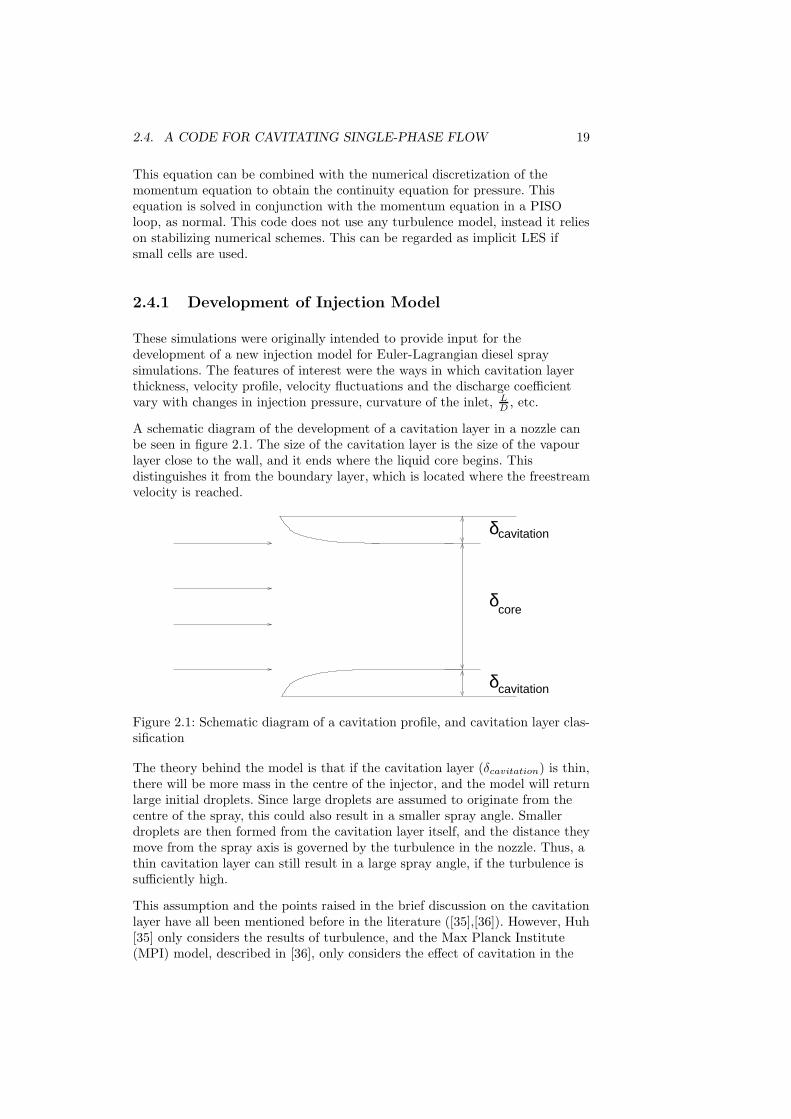
D , etc.
A schematic diagram of the development of a cavitation layer in a nozzle canbe seen in figure 2.1. The size of the cavitation layer is the size of the vapourlayer close to the wall, and it ends where the liquid core begins. Thisdistinguishes it from the boundary layer, which is located where the freestreamvelocity is reached.
δ
δ
δcavitation
cavitation
core
Figure 2.1: Schematic diagram of a cavitation profile, and cavitation layer clas-sification
The theory behind the model is that if the cavitation layer (δcavitation) is thin,there will be more mass in the centre of the injector, and the model will returnlarge initial droplets. Since large droplets are assumed to originate from thecentre of the spray, this could also result in a smaller spray angle. Smallerdroplets are then formed from the cavitation layer itself, and the distance theymove from the spray axis is governed by the turbulence in the nozzle. Thus, athin cavitation layer can still result in a large spray angle, if the turbulence issufficiently high.
This assumption and the points raised in the brief discussion on the cavitationlayer have all been mentioned before in the literature ([35],[36]). However, Huh[35] only considers the results of turbulence, and the Max Planck Institute(MPI) model, described in [36], only considers the effect of cavitation in the
20 CHAPTER 2. NOZZLE FLOW
nozzle. The aim of the new model was to account for both cavitation andturbulence, and to estimate their magnitude using CFD.
During the course of the project, several attempts were made to simulatecavitating diesel nozzle flow. Initially, the equation of state in the codeassumed that the vapour density was proportional to the pressure. The codeworked well for water injections into gas at atmospheric air pressures, but fordiesel pressures it caused the vapour density to rise above the liquid density.This forced the use of a unphysically high saturation pressure to avoidnegative pressures in the solution and allow the vapour density to remainbelow the liquid density. Attempts were made to extend this code to usePeng-Robinson equation of state (EOS) [37], but the EOS was not sufficientlysmooth to handle the large pressure gradients in the flow. The compressibilitymodel was also changed, from the Wallis [31] model to a linear compressibilitymodel. The change was necessary partly to enhance stability and partlybecause the same cavitation model was to be used for the multi-phase codehandling diesel vapour, liquid and air, as mentioned earlier. Since a linearcombination of the vapour fraction (γ) and liquid/gas fraction (α and β) ishighly suitable for describing the mixture’s properties in such cases, the samemodel was used for the single-phase code. A similar story of cavitation codedevelopment is reported in [38]. It starts off by using what the papers refers toas the Schmidt model [28], and ends in a modification of that model with acut-off for negative pressures.
The combined effects of these factors caused long delays in the simulations,and forced the author to limit the work to validating a model for cavitatingsingle-phase flow, without being able to develop a model for Lagrangian dieselspray simulations.1
1It should also be noted that it is only in special cases (mainly sprays with low evaporation,e.g. in cold starts) that the size of the initial droplets and their maximum spreading anglereally affect the combustion. This issue will be addressed in section 4.2.1
Chapter 3
Spray Modelling
In section 1.2, Lagrangian spray simulations were briefly described. Themethod used to introduce Lagrangian particles into an Eulerian grid issometimes called the discrete droplet model (DDM). This is based on the factthat we cannot resolve the full details of the near-nozzle flow using onlyEulerian cells (as yet at least). A typical nozzle has a diameter of around200 µm, so if it is to be resolved properly a cell size of about 20 µm is needed,but even if such small cells are only used around the injector the number ofcells required grows enormously if the calculations are run in 3D. Thus, thespray is usually modelled in some other way. There has been a growingnumber of attempts to simulate sprays using a full Eulerian approach, or byusing LES instead of the classical DDM with a k-ε turbulence model. Theseattempts are often associated with some limitations. For instance, de Villierset al [39] considers primary breakup close to a non-cavitating nozzle, Befrui etal [40] uses an updated version of the same code to study primary breakup innon-cavitating gasoline direct injection, and Menard et al [41] considers liquidinjection into incompressible air with a velocity of around 100 m/s. A spraystudy using LES and an Euler-Lagrangian description of the gas and liquidhas also been published, by Vuorinen et al [42]. They also used lower velocitiesthan those of diesel sprays and assumed the surrounding air to beincompressible, but the Reynolds number was comparable to those of dieselsprays. However, they did not simulate the near-nozzle behaviour, and mainlyfocused on studying the spray behaviour. All the papers mentioned above,ignore cavitation, and the simulations cover only part of the relevant physicaldomain.
One of the biggest problems associated with the DDM is modelling thenear-nozzle flow, more specifically the conditions close to the injector. In thisregion a liquid core forms from the liquid fuel being injected through theinjector. Ligaments are separated from this liquid core and form droplets thatevaporate and mix with the ambient gas. Hence, since the DDM assumesdisperse flow with spherical droplets of liquid, it is not an accuraterepresentation of the spray in this region. An option to improve near-injectorflow is to use the previously mentioned (in section 2.1) ELSA model. Aside
21
22 CHAPTER 3. SPRAY MODELLING
from the work by [24] (mentioned in 2.1), Blokkeel et al [43] and Lebas et al[44] have also used it to improve the primary breakup of the spray. Since theDDM model is only used when the liquid fraction is low, representing a statein which droplets (not ligaments) have been formed from the liquid core, themodel gives a better representation of the near-nozzle flow. Another benefit isthat such a modelling concept does not require a primary atomization model,and thus there are fewer model constants to tune. However, this raises some ofthe problems associated with high grid resolution to resolve the nozzlementioned earlier. There have also been other attempts to simulate spraysusing only Eulerian cells, in 2D ([45]). However, the Eulerian-Lagrangiandescription of the diesel spray has been the most widely used.
The large number of sub-models used to simulate the various physicalprocesses that the parcels are subjected to before they become part of the gascan pose further problems when using the DDM model. Each of these modelswill be thoroughly described later in this chapter, but here my intention is tomention the interactive problems they raise as a group. For instance, even ifthe breakup model is fully correct, the parcels can become too small due tothe evaporation model simulating evaporation too quickly, thus nullifying theexcellence of the breakup model. Similarly, a perfect turbulence interactioncan be ruined by a dissipative numerical scheme, or an overpredicting dragmodel that slows all the parcels down too much. Therefore, tuning the spraymodel in a non-combusting environment to constant volume experimentaldata, and then applying the results of the tuning to real engine calculationsoften yields poor results. The complex interactions amongst all of thesub-models make spray simulation somewhat more of an art than a science.
3.1 The Gas Phase
3.1.1 Basic Equations
The Eulerian grid is used to discretise the conservation equations of the fluidphase. When chemical reactions and interactions between the Lagrangian andEulerian phases are also involved, Eq. 2.8 needs to be extended to includeliquid spray evaporation. Furthermore, the density ρ becomes more complexsince diesel combustion involves multiple species, all of which affect thedensity. In addition, since chemical reactions are occuring various compoundswill be formed and participate in further reactions, so the mass fraction ofeach species is not conserved. However, if we consider the total density, theonly source term (ρs) is from spray evaporation.
∂ρ
∂t+ ∇ · (ρU) = ρs (3.1)
The evaporation source term is calculated from the evaporation sub-model,which will be described later. As already mentioned, each species will betransported, by both diffusion and convection, and may also be formed or
3.1. THE GAS PHASE 23
consumed by the reactions. The mass fraction for species i is denoted by Yi,and its transport equation is:
∂ρYi∂t
+ ∇ · (ρUYi) −∇ ((µ+ µT)∇Yi) = ρsi + κRRi (3.2)
ρs =∑
i
ρsi (3.3)
since most fuels consist of multiple species, and when combustion occurs theirnumber increases dramatically. For instance, when the mechanism including 83species was used for the calculations shown in Paper 3, the transport equationhad to be solved 83 times in each time iteration. The momentum equation alsoneeds to be modified due to the presence of a Lagrangian spray. Presentedhere is the equation for the mean velocities using a Reynolds Average NavierStokes assumption:
∂ρU
∂t+∇ ·
(ρUTU
)= −∇p+∇ ·
(
(µ+ µT)1
2(∇U + (∇U)T)
)
+ρg+Fs (3.4)
Fs is the spray momentum source term.
3.1.2 Turbulence Modelling
Since the goal of this project was to develop new models for industrialapplications, the turbulence was modelled using k-ε models. Paper 1 presentsconstant volume vessel simulations of diesel sprays conducted using threedifferent turbulence models, which yielded results that substantially differed interms of spray shape and penetration of liquid and vapour. For latersimulations different turbulence models were also tested, bearing in mind theintial results. The discrepancies between the models indicate the importance ofmodelling the turbulence correctly.
The three (compressible) models used in Paper 1 were: standard k-ε [46],Renormalized Group k-ε [47] (RNG) and Launder-Sharma’s k-ε (LS) [48]models. Each of the three turbulence models was developed with a differentrationale. The RNG model and the standard k-ε model used for these casesare both high Reynolds number models, meaning that they apply wallfunctions for the near wall cell. The Launder-Sharma turbulence model differsin this respect, since it is a low Reynolds number model, and has no wallfunctions. This places higher demands on the near-wall cell size, but since allcomputations in this work simulated events in a bomb, the near-wallbehaviour was not as important as the spray interactions by any of the wallsexcept the injector-wall.
The first turbulence model based on k and ε was originally presented in [46]. Itis shown in equations 3.5 and 3.6 in a general form to accommodate the threeturbulence models.
24 CHAPTER 3. SPRAY MODELLING
∂
∂t(ρk) + ∇ · (ρkU) −∇ · [(αkµT + µ)∇k] =
= 2µTS − 2
3ρk∇ ·U − ρε−Di (3.5)
∂
∂t(ρε) + ∇ · (ρεU) −∇ · [(αεµT + µ)∇ε] =
C12µTSε
k− 2
3C1ρε∇ ·U − C2ρ
ε2
k+ Bi (3.6)
where Bi and Di are listed below. Numerical constants and other variables arelisted in Paper 1.
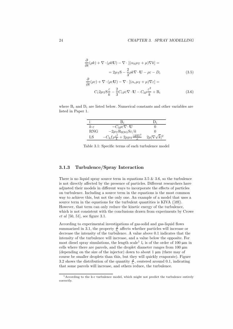
i Bi Di
k-ε −C3ρε∇ ·U 0RNG −2µTRRNGSε/k 0
LS −C2fρε2
k + 2µµT|∆U|2
ρ 2µ|∇√k|2
Table 3.1: Specific terms of each turbulence model
3.1.3 Turbulence/Spray Interaction
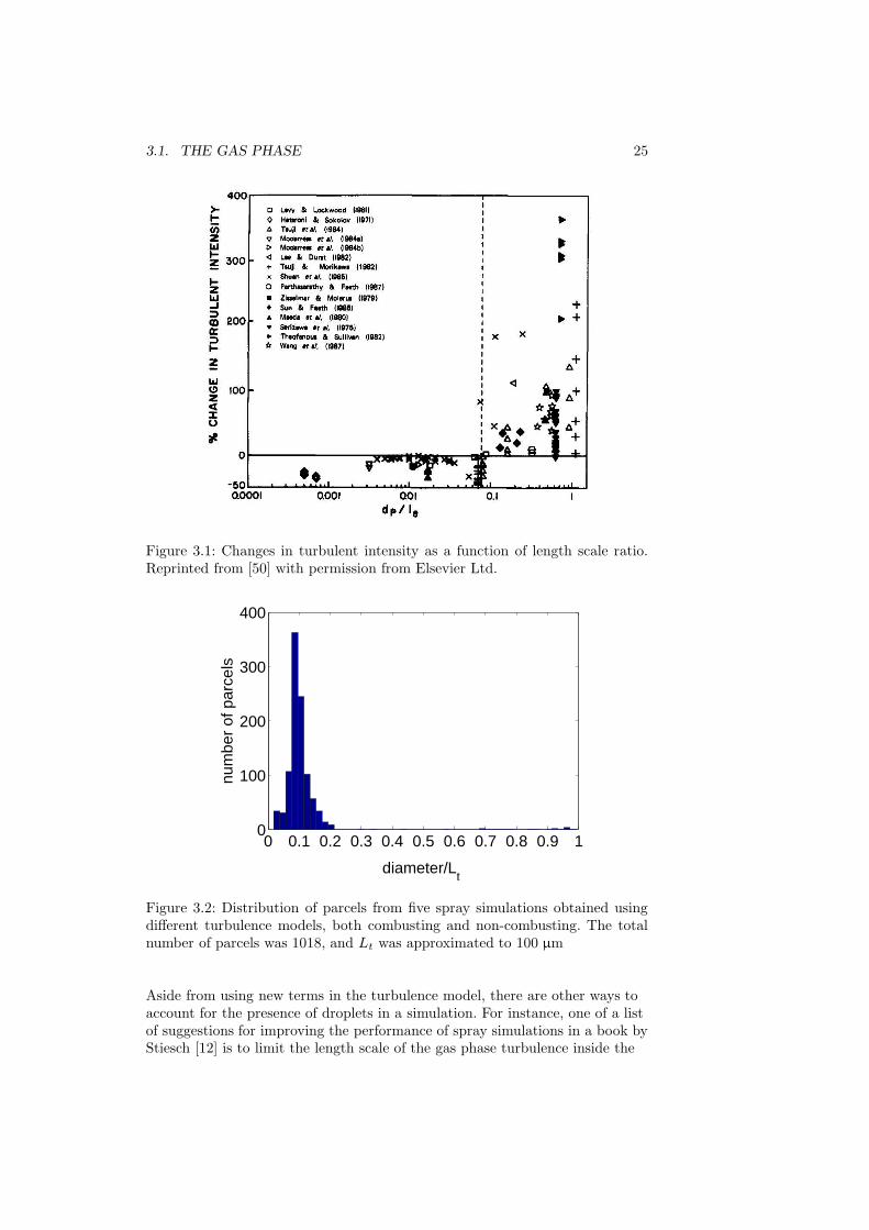
There is no liquid spray source term in equations 3.5 & 3.6, so the turbulenceis not directly affected by the presence of particles. Different researchers haveadjusted their models in different ways to incorporate the effects of particleson turbulence. Including a source term in the equations is the most commonway to achieve this, but not the only one. An example of a model that uses asource term in the equations for the turbulent quantities is KIVA ([49]).However, that term can only reduce the kinetic energy of the turbulence,which is not consistent with the conclusions drawn from experiments by Croweet al [50, 51], see figure 3.1.
According to experimental investigations of gas-solid and gas-liquid flowssummarized in 3.1, the property d
ltaffects whether particles will increase or
decrease the intensity of the turbulence. A value above 0.1 indicates that theintensity of the turbulence will increase, and a value below the opposite. Formost diesel spray simulations, the length scale1 lt is of the order of 100 µm incells where there are parcels, and the droplet diameter ranges from 100 µm(depending on the size of the injector) down to about 1 µm (there may ofcourse be smaller droplets than this, but they will quickly evaporate). Figure3.2 shows the distribution of the quantity d
lt, centered around 0.1, indicating
that some parcels will increase, and others reduce, the turbulence.
1According to the k-ε turbulence model, which might not predict the turbulence entirelycorrectly.
3.1. THE GAS PHASE 25
Figure 3.1: Changes in turbulent intensity as a function of length scale ratio.Reprinted from [50] with permission from Elsevier Ltd.
0 0.1 0.2 0.3 0.4 0.5 0.6 0.7 0.8 0.9 10
100
200
300
400
diameter/Lt
num
ber
of p
arce
ls
Figure 3.2: Distribution of parcels from five spray simulations obtained usingdifferent turbulence models, both combusting and non-combusting. The totalnumber of parcels was 1018, and Lt was approximated to 100 µm
Aside from using new terms in the turbulence model, there are other ways toaccount for the presence of droplets in a simulation. For instance, one of a listof suggestions for improving the performance of spray simulations in a book byStiesch [12] is to limit the length scale of the gas phase turbulence inside the
26 CHAPTER 3. SPRAY MODELLING
spray to the jet diameter in order to reduce the grid dependency of thecalculations. Such a modification would also cause the turbulence model to beaffected by the particles. However, the suggestion raises several problems.Notably, the jet diameter is not well defined, it could refer solely to the liquidpart of the spray, or the vapour part could also be included. Similarly, theterm “inside the spray”, could refer to just the liquid core, or include thevapour cloud.
The author chose to limit the turbulent length scale to the nozzle diameter incells with parcels. The spray is a cloud of parcels, and all cells that haveparcels in them must be inside this cloud. There can be cells that do not havea parcel in them, but if we choose a high number of injected parcels there willbe few such cells. The nozzle diameter is selected rather than the jet diameterbecause the nozzle diameter is the parameter that initially sets the lengthscale of the turbulence. Fixing the limit prevents the turbulence length scalefrom growing, but it also simplifies the calculations, since calculating the jetdiameter in every timestep would be costly. Thus, the nozzle diameter is agood first approximation.
k governs the scale of the fluctuating turbulent velocity, and ε the size of theturbulent eddies. The limit was thus imposed on ε. The length scale of theturbulence is defined as:
lt = Cµk3/2
ε(3.7)
Thus, since the limit was imposed on ε, it was limited by:
Cµk3/2
Lsgs< ε (3.8)
Where Lsgs is set to the nozzle diameter. The constraint is imposed after theequations for k and ε are solved. If the constraint is applied before any of theequations are solved, the constraint in equation 3.8 cannot be guaranteed.
The modification of the turbulence model implies an assumption regarding ε;that the equation for ε underestimates the dissipation when liquid parcels arepresent. One could also think of this as over-prediction of the length scale ofthe spray, which is perhaps easier to imagine, and this explanation will be usedin the rationale below.
The parcels in a diesel spray problem have fairly high velocities, and theincreased momentum of the gas comes from the spray. Thus, the resultinglength scale of the turbulence should also be governed by the spray and nozzlesize, which is what this modification does. One could argue that this only shiftsthe dependency from the grid to the magnitude of the turbulence length scalelimit. While this is true, it is a much cheaper dependency computationally.
3.1. THE GAS PHASE 27
3.1.4 Chemistry
After the fuel liquid droplets have undergone breakup and evaporation, thefuel mixes with the surrounding air and forms a combustible mixture. A realdiesel fuel consists of about 1000 different species, reacting with the air in over10 000 reactions. Thus, when studying combustion, either experimentally ornumerically, the complexities are generally reduced by considering thecombustion of a simpler model fuel. One such model fuel is n-heptane, anotheris the IDEA model fuel consisting of n-decane and α-methyl-naphthalene.Both have been used in this work: IDEA for the spray studies described inPaper 1, and n-heptane for the studies described in Papers 3 and 4.
Solving the chemistry numerically means solving a large system of reactionequations. For each reaction
Sf11[X1] + Sf
21[X2] + ... −→ Sr11[X1] + Sr
21[X2] + ... (Re. 1)
there is a corresponding reaction rate equation which determines how rapidlythe reaction is proceeding and in which direction. To formulate the reaction ina more general manner, reaction j is written as:
Ns∑
i=1
Sfij[Xi]
kfj
krj
Ns∑
i=1
Srij[Xi] (Re. 2)
where Sf and Sr are the matrices of forward and reverse stoichiometriccoefficients, respectively, kfj and krj are the corresponding reaction rateconstants of reaction j, and [Xi] is the molar concentration of species i in thecell. The matrix of stoichiometric coefficients consists of Ns rows, with therows corresponding to species. The columns represent reactions, making thematrix Ns ×Nr. The reaction rate constant k is itself a function of theArrhenius constants:
kj = AjTβje−
Ea,jRT (3.9)
which need to be specified as part of the mechanism. It is now possible towrite the equation for the reaction rate of the basic reaction, Re. 1. The rateof formation of species [X1] from reaction j is written as:
(d[X1]
dt
)
j
= Sr1j
(
kfj
Ns∏
i=1
[Xi]Sf
1j − krj
Ns∏
i=1
[Xi]Sr
1j
)
(3.10)
This equation is formulated for every species included in the chemicalmechanism, as well as for every reaction, resulting inn an equation system
28 CHAPTER 3. SPRAY MODELLING
consisting of Ns ×Nr equations. As can be seen from the above equation, it isa system of Ordinary Differential Equations (ODEs), which can be solvedcoupled using an ODE solver, sequentially using a reference species technique[52], or by an Euler-Implicit method. OpenFOAM has the ability to solve theequations using an ODE solver (an approach used in Paper 3). Some versionsof KIVA-3V also offer the option of solving the chemical rate reactionscoupled, one of them being the KIVA-3V version also used in Paper 3. Asidefrom the concentrations, it is also important to find the right hand side ofequation 3.10, since it is used in the source term in the transport equation(equation 3.2). The source term for species i is:
RRi =Wi
ρ
Nr∑
j=1
(Srij − Sfij)ωj (3.11)
ωj = kfj
Ns∏
i=1
[Xi]Sf
ij − krj
Ns∏
i=1
[Xi]Sr
ij (3.12)
As mentioned, a real mechanism for hydrocarbon fuels (including model fuels)would be very large. While it is possible to use such mechanisms in shock tubesimulations, they are too large to use in a CFD simulation. As mentioned inthe above section, each reaction requires a term describing the amounts ofeach species it forms, and each species requires a transport equation to besolved. One example of a sufficiently small mechanism is the reduced one usedin Paper 3, consisting of 338 reactions and 83 species. This mechanism has tosolve 83 systems of ODEs in every cell, in every timestep. Some of theequations in the system will not be applicable, since no reaction includes allspecies, but in theory the system could comprise 28054 ODEs in total.
To solve the chemical reaction equations, a stiff ODE solver is needed. The oneused in the studies presented in Paper 3 is the SIBS method (Semi-ImplicitBulirsch Stoer [53]) in OpenFOAM, which is based on Richardsonextrapolation of the approximated solution. As mentioned earlier the solverneeds to solve ODEs in every timestep to determine the chemical species’concentrations at the end of the timestep. The Richardson extrapolation of thefunction y assumes that as the interval (in our case the computational timestep∆t) is split up into increasing number of sub-steps, the solution will convergeto some value y∞. However, the solver will never apply enough sub-steps tofind it. Instead, it will approximate it, depending on the solution using largesub-steps. The analytical function used to approximate y∞ is a polynom, andthe error function of the method contains only even terms of the step size.
Chalmers PaSR Model
It is necessary to use some form of treatment for the chemistry and turbulentmixing, in the literature there are many suggestions for doing this, including:PaSR ([54]), diffusion flamelets [55], detailed chemical kinetics with aperfectly-stirred reactor [56], and the general flame surface density model [57].
3.1. THE GAS PHASE 29
However, the Chalmers PaSR model was used to model the turbulence -chemistry interaction in Paper 3.
The PaSR model is based on the theory that real flames are much thinnerthan any computational cell, so assuming that an entire cell is a perfectreactor is a severe overestimation. Thus, the cells are divided into a reactingpart, and a non-reacting part. The reacting part is treated like a perfectlystirred reactor, in which all present species are homogeneously mixed andreacted. After reactions have taken place, the species are assumed to be mixeddue to turbulence for the mixing time τmix, and the resulting concentrationgives the final concentration in the entire, partially stirred, cell. The relativesizes of the parts of the computational cell constituting the reactor and therest of the cell, are governed by the turbulent mixing time and the residencetime (the numerical time step, τ , in our case). The reaction rate term forspecies i is then approximated as:
∂ci
∂t=ci1 − ci0τ
= κRRi(ci1) (3.13)
Where RRi(ci1) is the laminar chemical source term, and κ the reaction rate
multiplier, defined as:
κ =τc
τc + τmix(3.14)
where τmix is the turbulence timescale mentioned above, and τc thecorresponding chemical timescale. This factor appears in the species transportequation with the chemical source term (as in equation 3.2):
∂ρYi∂t
+ ∇ (ρYiU) −∇ (µEff∇ (Yi)) =
= Si + κRRi(ci) (3.15)
where τmix is the turbulence timescale mentioned above, it is assumed to bedetermined by k and ε:
τmix = Cmixk
ε(3.16)
with Cmix = 0.03. The chemical timescale is determined by solving thereaction system’s ODEs fully coupled, and finding the characteristic time forthat system. Other variations and detailed derivations of the PaSR model canbe found in [52, 54, 58, 59].
30 CHAPTER 3. SPRAY MODELLING
3.2 Spray Sub-Models
3.2.1 Spray Motion Equation
The motion of a Lagrangian particle, moving in an Eulerian framework, isgoverned by one of the most fundamental laws of physics; Newton’s second law:
∂pd
∂t=∑
i
Fi (3.17)
Unfortunately, this equation cannot be solved immediately, simply because theforce acting on the parcel is unknown. The full spray equation, often referredto as the BBO equation - from Basset (1888), Boussinesq (1903) andOseen(1927) - includes effects of added mass, pressure, Basset force2, Magnuseffect3, Saffman force4, and Faxen5 force. They are all neglected. Most of theterms can be neglected due to the high density ratio between the two phases,while others like the Magnus effect are neglected since rotation of the dropletswill not be very important. What remains are the forces due to drag andgravity acting on the droplets. The latter is included for simplicity and theformer due to its physical importance. These simplifications allow us to writethe right hand side of equation 3.17 as:
∂pd
∂t= −ρg
πD2
8CD (ud −U) |ud −U| + ρd
πD3
6g (3.18)
This equation can be simplified further, if we assume the droplets arespherical, and that the drag will not be affected by changes in mass, then:
∂pd
∂t= md
∂ud
∂t= ρd
πD3
6
∂ud
∂t(3.19)
A droplet’s mass will of course change with time (due to breakup &evaporation), but we assume that the changes will not affect the drag. Thismeans we can neglect the effect that causes rockets to liftoff and airplanes tofly, an effect that is not believed to be pronounced in diesel droplets from whichsome mass is evaporating. If we combine equations 3.18 and 3.19, the result is:
∂ud
∂t= −3
4
ρg
ρd
1
DCD (ud −U) |ud −U| + g (3.20)
To simplify this equation further, a momentum relaxation time is introduced:
2This is the force that causes a motorboat to continue in its path even when the motor hasbeen switched off recently.
3The force that causes a soccer ball to rotate perfectly past defenders and into the net4Lift force due to shear5force due to curvature of the flow
3.2. SPRAY SUB-MODELS 31
τu =8md
πρgCDD2|ud − u| =4
3
ρdD
ρgCD|ud − u| (3.21)
Equation 3.20 can now be written as:
∂ud
∂t= −ud −U
τu+ g (3.22)
Even with the introduction of τu, the drag cannot be approximated without adrag coefficient, which will be introduced in a later section in this chapter.
3.2.2 Parcel Tracking
In Lagrangian spray simulations, the particles representing liquid are movingin a fixed Eulerian framework as described above. Tracking them and definingthe cells they are in are clearly important issues. There are two main ways ofdoing this, one called the Lose-Find algorithm, and one called theFace-To-Face algorithm.
The Lose-find algorithm is fairly simple and can be described in four steps.
1. Update the properties of the parcel2. Move the parcel with velocity ud for time ∆t3. Find out which cell the parcel is in4. Add momentum to the cell to which the parcel has moved
Assuming that the time step is sufficiently small to ensure that every parceltraverses more than one cell, this approach is acceptable. However, even for asmall time step, a parcel can still be moved across a cell without having anymomentum exchange with it. The model is used in KIVA-3V, as well as somecommercial CFD codes. Due to the problems mentioned above, however,another model is used in OpenFOAM; Face-To-Face tracking. It too can bedescribed in four steps:
1. Move the parcel until it reaches a cell boundary or for theentire time step ∆t if it remains in the same cell
2. If the parcel changes cell, calculate the time it took to moveout of the first cell, and update the parcel properties
3. Add the momentum-change to the cell that the parcel hasbeen in
4. If the parcel still has time left to move, go back to 1.
The Face-To-Face tracking in OpenFOAM includes a stability check thatbegins by tracking the parcel from the centre of the cell it belongs to, ratherthan from the particle’s position. This is done to ensure that particles thatmight be close to the edge of the cell (or even slightly outside) are properlytracked.
32 CHAPTER 3. SPRAY MODELLING
Parcels tracked by Face-To-Face tracking cannot ’skip’ cells, which improvesthe predictions of transfer of mass, momentum and energy. For a more detaileddescription, see [60].
3.2.3 Injection Model
The injection model used in the Lagrangian spray simulations is a solid-coneinjection model. The user supplies a drop diameter probability densityfunction (PDF) with parameters, in this case a Rosin-Rammler form waschosen. The model also requires minimum and maximum values for the dropletsize, as well as the maximum spray cone angle. The parameters for the modelcan be found in table 3.2
Model parameter Numerical Valuedmin 10−6 mdmax dnozzle
dmean dnozzle
n 3βmax 20
Table 3.2: Solid cone injection model constants
The direction of a droplet to be injected into the domain is calculated bymultiplying βmax and a random number between 0 and 1. This angle is theangle between the set spray direction and the direction of the injected droplet.Note that βmax is not the half-angle of the spray, but the full spray angle. Thevelocity of the injected parcel is based on the injection pressure, and thepressure in the domain:
ud = Cd
√
2∆p
ρi(3.23)
where ρi is the density of the injected parcel, taking the type of fuel, injectionpressure, and composition of fuel (for multi-component fuels) into account. Cdis the discharge coefficient, a parameter that varies from nozzle to nozzle, andis to a certain degree pressure-dependent [15].
3.2.4 Drag Model
Several options for the drag coefficient have been suggested in the literature([36],[61],[62]), but the one chosen here was:
CD =
24Red
(
1 +Re
23d
6
)
Red < 1000
0.44 Red > 1000
(3.24)
3.2. SPRAY SUB-MODELS 33
OpenFOAM also offers the possibility to account for changes in drag due tooscillations of the droplet surface, i.e. the instability waves eventually resultingin droplet breakup. If this model is used, the TAB model [9] will be used tocalculate the oscillations and the resulting drag will be added to the dragdescribed above. The modification is
CD = CD,model(1 + CD,distortmin(ylim, y)) (3.25)
where CD,distort and ylim are user-set constants, and y is the relative deviationfrom the equator of the parcel if it were spherical. ylim is usually set to 1.0.The minimum function is not necessary when the TAB breakup model is used,since a y-value of 1.0 will result in the parcel breaking up.
3.2.5 Breakup Model
The breakup model used is the Kelvin-Helmholtz-Rayleigh-Taylor (KHRT)model ([8] & [63]). This model, along with the TAB model, is one of the mostwidely used models in Lagrangian spray simulations today ([64],[65],[66]). TheKHRT model was chosen for its superior performance under diesel conditions([67]). It is also possible to use the TAB model, but often in conjunction withsome form of atomization model since the TAB model tends to break up thedroplets very rapidly. The KHRT model includes two modes of breakup: KHbreakup, accounting for unstable waves growing on the liquid jet due to thedifferences in velocity between the gas and liquid; and RT breakup, accountingfor waves growing on the droplets’ surface due to acceleration normal to thedroplet-gas interface. Analysis of a round liquid jet yields a fastest growingwave with a wavelength (ΛKH) and a growth rate (ΩKH):
ΛKH = 9.02r(1 + 0.45Oh
12 )(1 + 0.4Ta0.7)
(1 + 0.865We1.67)0.6(3.26)
ΩKH =(0.34 + 0.38We
32 )
(1 + Oh)(1 + 1.4Ta0.6)
√σ
ρdr3(3.27)
The critical droplet radius rc, which is the radius a parcel will have after it hasbeen stripped off the liquid jet, is assumed to depend linearly on thewavelength ΛKH and the stripping rate, or characteristic breakup time τKH
(which controls the breakup rate) is assumed to be a simple function of thegrowth rate ΩKH, wave-length ΛKH and droplet radius, r:
rc = B0ΛKH (3.28)
τKH =3.726B1r
ΩKHΛKH(3.29)
The continuous reduction of droplet size due to breakup can then be definedby the rate equation:
34 CHAPTER 3. SPRAY MODELLING
dr
dt= −r − rc
τKH(3.30)
which essentially describes how rapidly the drops will reach the stable state.The breakup parameters B0 and B1 can be found in Table B.1. In addition tothese two constants, there are two more parameters to control the KHbreakup. The first determines whether breakup will occur at all. IfWe < Welimit, the drop has reached a stable state and no breakup due toKelvin Helmholtz instabilities will occur. The second parameter controls therate of introduction of new child-parcels. As the jet breaks up the parcel willaccumulate a stripped mass, ms, and when ms exceeds a certain percentage ofthe average parcel mass, which is the total injected liquid mass divided by thetotal number of injected parcels, a new parcel will be introduced with size rc,containing the accumulated mass ms.
Rayleigh-Taylor breakup, on the other hand, is governed by how rapidlydisturbances grow on the surface of the droplet. For real droplets thesedisturbances originate from the droplets’ trailing edges [12]. If thesedisturbances are assumed to be linear, the frequency of the fastest growingwave, and the corresponding wavelength, is given by:
ΩRT =
√
2|gt(ρl − ρg)|1.53√
3σ(ρg + ρl)(3.31)
gt = (g +dud
dt) · ud
|ud|(3.32)
ΛRT = 2πCRT
√
3σ
|gt(ρl − ρg)|(3.33)
Where CRT is a modelling parameter. If this wavelength of the fastest growingwave is smaller than the diameter of the droplet diameter and theperturbations are allowed to grow for a period of time, the droplet will beimmediately converted into a parcel with smaller droplets when the growthtime exceeds the characteristic RT time. The new size is proportional to thewavelength ΛRT of the disturbances. Thus, CRT determines both whether ornot the droplets are going to be converted into smaller drops and how largethe new droplets are going to be. The RT mode does not add any new parcelsto the system, it only increases the statistical number of droplets in the parceland changes the radii of the droplets.
3.2.6 Evaporation Model
When modelling the evaporation of a droplet, the key parameter is thelifetime, or evaporation relaxation time of the droplet. The derivation of thistime starts by evaluating the time-derivate of the mass of the droplet.
3.2. SPRAY SUB-MODELS 35
dmd
dt= ρd
d
dt
(
4
3π
(D
2
)3)
=ρdπ
2D2 dD
dt(3.34)
Further, the evaporation is assumed to follow the empirical D2-law:
dD2
dt= Ce ⇒
dD
dt=
Ce
2D(3.35)
where Ce is a constant. From this equation we can determine the relaxationtime by integration (since Ce is a constant).
D2 = Cet+D2o (3.36)
If we want to determine the time (τe) when a droplet of size D0 has completelyevaporated, we can put D = 0 into the above equation, resulting in:
τe = −D20
Ce(3.37)
The only unknown in this equation is the constant Ce, which will bedetermined by inserting equation 3.35 into equation 3.34, the result is:
dmd
dt=ρdπ
4DCe (3.38)
However, the time derivative of the mass of the droplet can also be expressedas ([52]):
dmd
dt= −πDShDρvln
(p− pv,∞
p− pv,s
)
=
= −πDShDρvln
(
1 +Xv,s −Xv,∞
1 −Xv,s
)
(3.39)
Using these two equations for dmd
dt , the value of the constant Ce can beexpressed as:
Ce = −4Shρv
ρdDln
(
1 +Xv,s −Xv,∞
1 −Xv,s
)
(3.40)
The Sherwood number Sh is calculated using the Ranz-Marshall (or Frossling)correlation (from [51]):
Sh = 2 + 0.6Re1/2Sc1/3 (3.41)
36 CHAPTER 3. SPRAY MODELLING
Equation 3.37 can now be used with known Ce to solve equation 3.39:
dmd
dt= −md
τe(3.42)
where the relaxation time is
τe =ρdD
2
6DShρvln(
1 +Xv,s−Xv,∞
1−Xv,s
) (3.43)
and a similar equation for the diameter (from 3.35):
dD
dt= − D
3τe(3.44)
A relaxation time is introduced to characterise the evolution of the particlesize. If an explicit method is used, the time step (a function of the relaxationtimescale) must not be larger than the relaxation time, or the mass willbecome negative. If an implicit method is used, the method is unconditionallystable. It is also consistent with the way the momentum and heat transferequations for each parcel are solved. The difference in timescales of theseprocesses is useful for determining the rate at which each process is proceeding.
3.2.7 Heat Transfer
The heat transfer model comes in part from [51], and is based on theconvective heat transfer of a particle with a uniform temperature. Amodification was made to account for the latent heat phase transfer duringevaporation. The heat transfer model also uses the evaporation relaxationtime, since the evaporation of a droplet also transfers heat to the surroundinggas.
dTd
dt=πDκcNu
mdcl(Tg − Td) fheat −
1
cl
hv(Td)
τe(3.45)
The modification is in the factor fheat which is:
fheat =− cp,vmd
πDκcNu(
e−cp,vm
πDκcNu − 1) (3.46)
The first part of equation 3.45 accounts for the heat transfer to the liquid, andthe second part for latent heat arising from mass transfer. Since the masstransfer is related to the evaporation of the droplet, the relaxation timeintroduced in 3.2.6 is used. The heat transfer can also be expressed with arelaxation time:
3.2. SPRAY SUB-MODELS 37
τh =mdcl
πDκcNu(3.47)
resulting in:
dTd
dt=
(Tg − Td)
τhf − 1
cl
hv(Td)
τe(3.48)
where one term describes heat transfer due to temperature difference, and theother heat transfer due to mass of the droplet lost through evaporation.
3.2.8 Particle Collisions
OpenFOAM offers two collision models: the O’Rourke model [68], and themodification by Nordin [52]. Other models have also been published, forinstance the collision model by Schmidt et al [69], using adaptive collisionmeshing, which involves generating a separate orthogonal collision mesh withrandom orientation in every time step. The mesh is refined until the number ofparcels in each cell is below a set threshold.
In the simulations presented in the included papers and the results chapter thetrajectory collision model by Nordin [52] was used (unless otherwise stated).This is based on the O’Rourke collision model, which will be briefly described.Other modifications have also been made to the O’Rourke model [70]. In theoriginal version, parcels collide if they are in the same cell with a probabilitygiven by:
e−min(N1,N2)
14Vcell
π(d1+d2)2|U1−U2|∆t (3.49)
In practice, a random number between 0 and 1 is generated for each parcel. Ifthe number is lower than the probability, the parcels are set to collide. Theoutcome of the collision depends on the Weber number, resulting in eithercoalescence or grazing. Thus, the direction of the parcels has no influence onwhether they collide or not, nor does their position within the cell. If the cellsare large, parcels several droplet radii away will be able to collide, althoughthe probability of this will be lower, according to equation 3.49 (due to thelarge cell size). At the other extreme, there will be few collisions in very smallcells, since parcels will not often occupy the same cell. In all, the O’Rourkemodel has very strong grid dependency, as shown in [52, 69].
As mentioned previously, the model implemented into OpenFOAM used forthe work presented in the appended papers is a modified form of the O’Rourkemodel. Instead of only colliding parcels that are in the same cell, the algorithmcalculates the paths of all parcels and collides those that will intersect withinthe same timestep. Thus the parcels need to be in the same position,regardless of the mesh. Since a simulated spray may contain several thousandparcels, the algorithm first calculates whether a pair of parcels is heading
38 CHAPTER 3. SPRAY MODELLING
towards each other. If they are not, they are regarded as not colliding. Thisreduces the computational load of the algorithm, and is done by computing:
vAlign =(U1 −U2) · (x2 − x1)
|x2 − x1|(3.50)
This property will give how much of the vector x2 − x1 can be projected ontothe vector U1 −U2, if it is positive it indicates that the parcels are headingtowards one another, if it is negative they are travelling away from each other,and if it is zero, they are on a perpendicular course. The parcels also need tobe close enough to collide since, as mentioned before, they need to reach eachother within the current timestep, this gives the next criterion:
|x2 − x1| −d1 + d2
2< vAlign∆t (3.51)
On the left hand side of this equation is the distance between the dropletsurfaces, and on the right hand side the parcels’ relative displacement duringthe current timestep, which must be larger. This ensures that the parcels canreach each other within the given time (the numerical timestep). The questionthat remains to resolve is whether or not the parcels reach the intersection atthe same time. If, for instance, one parcel has a high velocity and the other alow velocity, they may miss each other. So the algorithm needs to determinethe times (designated tα and tβ) at which the parcels reach the intersection,this is done by solving:
x1,new = x1 + tU1 x2,new = x2 + tU2 (3.52)
∂|x2,new − x1,new|∂t1
(t = tα) = 0∂|x2,new−x1,new|
∂t2(t = tβ) = 0 (3.53)
Whether the parcels actually collide or not is governed by chance, theprobability for a collision is now given by:
Pcoll =
( 12 (d1 + d2)
max( 12 (d1 + d2), |x1,new(tα) − x2,new(tβ)|)
)Cspace
e−ctime|tα−tβ |
∆t
(3.54)
where |x1,new − x2,new| is the smallest distance between the two parcels duringthe timestep. As this value declines, the probability of collision increases. Thetwo model constants Ctime and Cspace control the collision rate in time andspace, respectively.
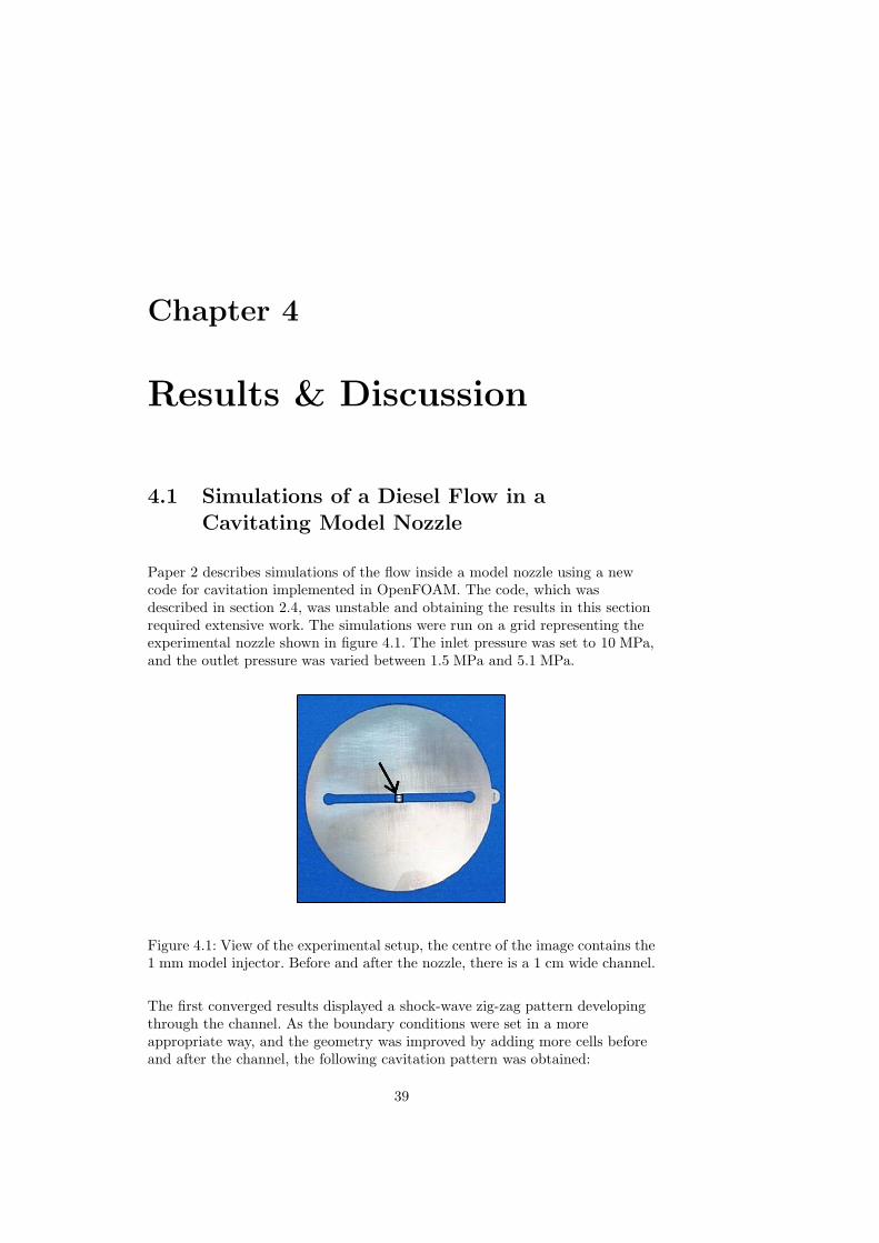
Chapter 4
Results & Discussion
4.1 Simulations of a Diesel Flow in a
Cavitating Model Nozzle
Paper 2 describes simulations of the flow inside a model nozzle using a newcode for cavitation implemented in OpenFOAM. The code, which wasdescribed in section 2.4, was unstable and obtaining the results in this sectionrequired extensive work. The simulations were run on a grid representing theexperimental nozzle shown in figure 4.1. The inlet pressure was set to 10 MPa,and the outlet pressure was varied between 1.5 MPa and 5.1 MPa.
Figure 4.1: View of the experimental setup, the centre of the image contains the1 mm model injector. Before and after the nozzle, there is a 1 cm wide channel.
The first converged results displayed a shock-wave zig-zag pattern developingthrough the channel. As the boundary conditions were set in a moreappropriate way, and the geometry was improved by adding more cells beforeand after the channel, the following cavitation pattern was obtained:
39
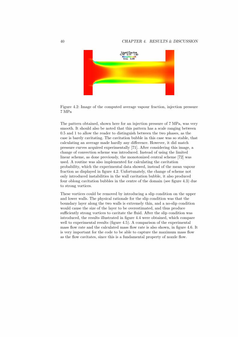
40 CHAPTER 4. RESULTS & DISCUSSION
Figure 4.2: Image of the computed average vapour fraction, injection pressure7 MPa
The pattern obtained, shown here for an injection pressure of 7 MPa, was verysmooth. It should also be noted that this pattern has a scale ranging between0.5 and 1 to allow the reader to distinguish between the two phases, as thecase is barely cavitating. The cavitation bubble in this case was so stable, thatcalculating an average made hardly any difference. However, it did matchpressure curves acquired experimentally [71]. After considering this image, achange of convection scheme was introduced. Instead of using the limitedlinear scheme, as done previously, the monotonized central scheme [72] wasused. A routine was also implemented for calculating the cavitationprobability, which the experimental data showed, instead of the mean vapourfraction as displayed in figure 4.2. Unfortunately, the change of scheme notonly introduced instabilities in the wall cavitation bubble, it also producedfour oblong cavitation bubbles in the centre of the domain (see figure 4.3) dueto strong vortices.
These vortices could be removed by introducing a slip condition on the upperand lower walls. The physical rationale for the slip condition was that theboundary layer along the two walls is extremely thin, and a no-slip conditionwould cause the size of the layer to be overestimated, and thus producesufficiently strong vortices to cavitate the fluid. After the slip condition wasintroduced, the results illustrated in figure 4.4 were obtained, which comparewell to experimental results (figure 4.5). A comparison of the experimentalmass flow rate and the calculated mass flow rate is also shown, in figure 4.6. Itis very important for the code to be able to capture the maximum mass flowas the flow cavitates, since this is a fundamental property of nozzle flow.
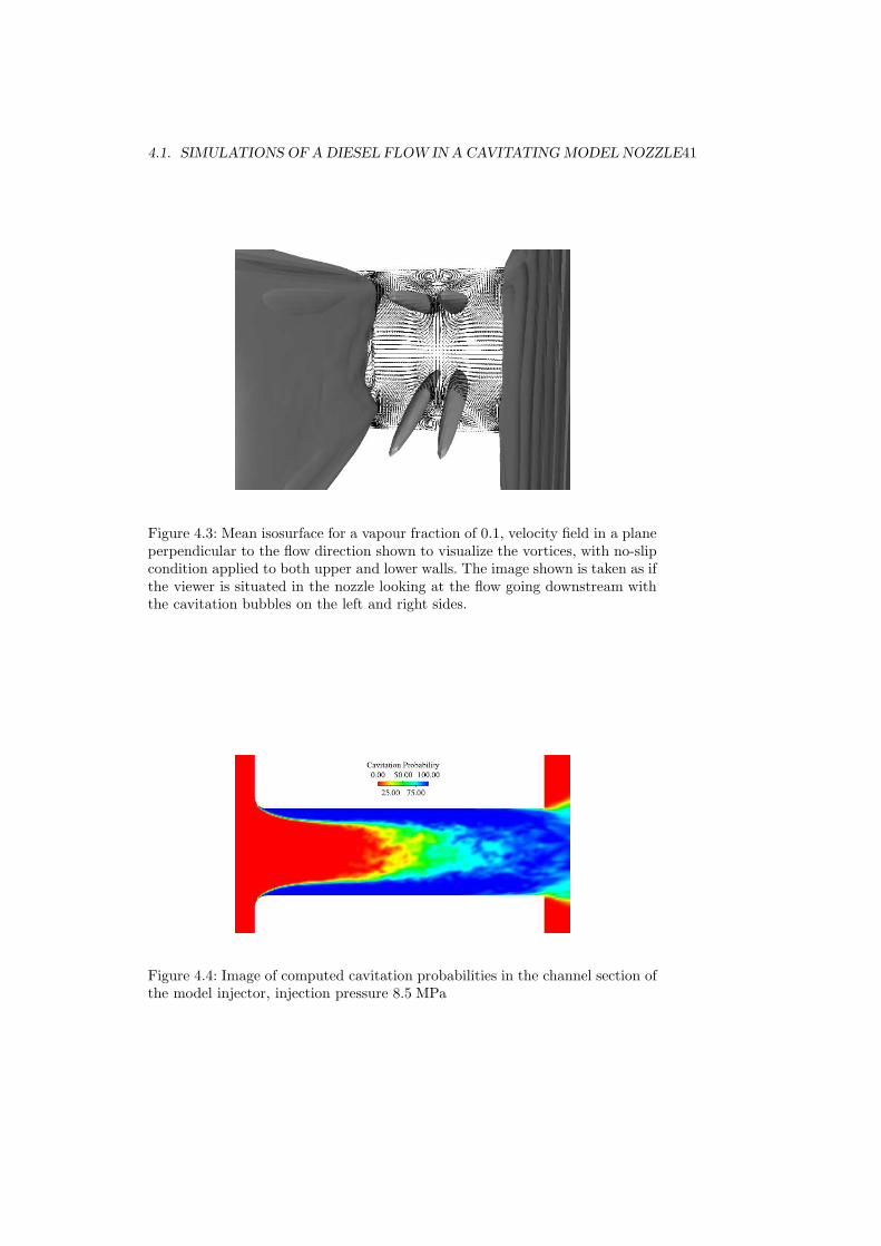
4.1. SIMULATIONS OF A DIESEL FLOW IN A CAVITATING MODEL NOZZLE41
Figure 4.3: Mean isosurface for a vapour fraction of 0.1, velocity field in a planeperpendicular to the flow direction shown to visualize the vortices, with no-slipcondition applied to both upper and lower walls. The image shown is taken as ifthe viewer is situated in the nozzle looking at the flow going downstream withthe cavitation bubbles on the left and right sides.
Figure 4.4: Image of computed cavitation probabilities in the channel section ofthe model injector, injection pressure 8.5 MPa
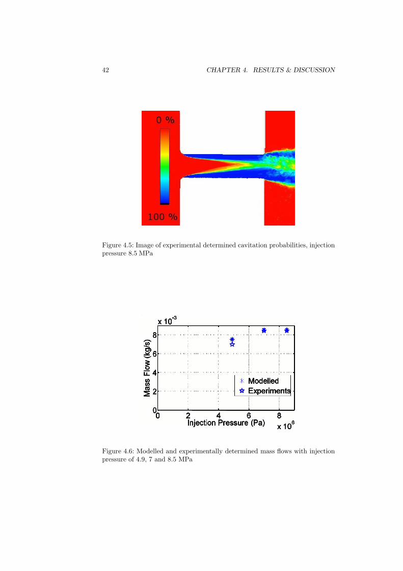
42 CHAPTER 4. RESULTS & DISCUSSION
Figure 4.5: Image of experimental determined cavitation probabilities, injectionpressure 8.5 MPa
Figure 4.6: Modelled and experimentally determined mass flows with injectionpressure of 4.9, 7 and 8.5 MPa
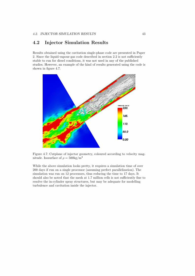
4.2. INJECTOR SIMULATION RESULTS 43
4.2 Injector Simulation Results
Results obtained using the cavitation single-phase code are presented in Paper2. Since the liquid-vapour-gas code described in section 2.2 is not sufficientlystable to run for diesel conditions, it was not used in any of the publishedstudies. However, an example of the kind of results generated using the code isshown in figure 4.7.
Figure 4.7: Cutplane of injector geometry, coloured according to velocity mag-nitude. Isosurface of ρ = 500kg/m3
While the above simulation looks pretty, it requires a simulation time of over200 days if run on a single processor (assuming perfect parallelization). Thesimulation was run on 12 processors, thus reducing the time to 17 days. Itshould also be noted that the mesh at 1.7 million cells is not sufficiently fine toresolve the in-cylinder spray structures, but may be adequate for modellingturbulence and cavitation inside the injector.
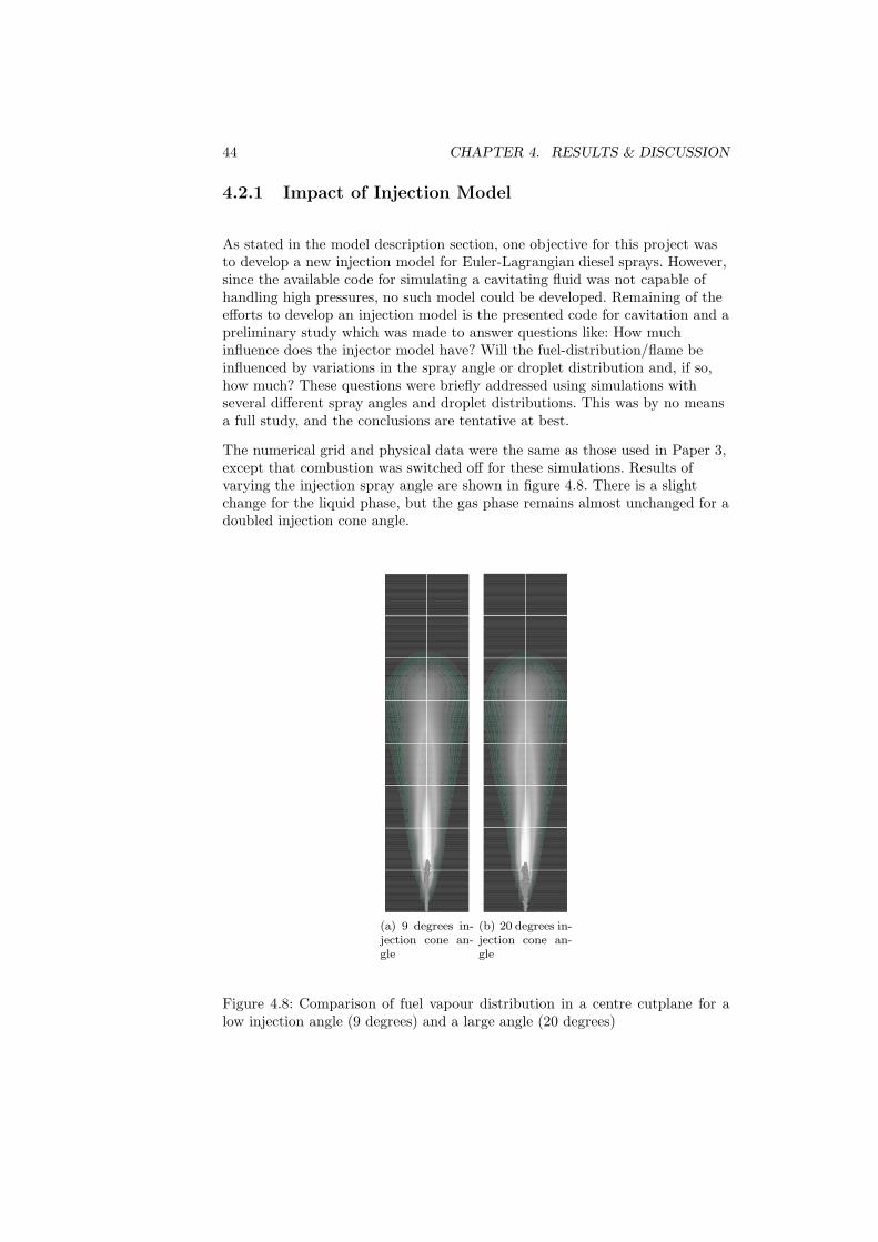
44 CHAPTER 4. RESULTS & DISCUSSION
4.2.1 Impact of Injection Model
As stated in the model description section, one objective for this project wasto develop a new injection model for Euler-Lagrangian diesel sprays. However,since the available code for simulating a cavitating fluid was not capable ofhandling high pressures, no such model could be developed. Remaining of theefforts to develop an injection model is the presented code for cavitation and apreliminary study which was made to answer questions like: How muchinfluence does the injector model have? Will the fuel-distribution/flame beinfluenced by variations in the spray angle or droplet distribution and, if so,how much? These questions were briefly addressed using simulations withseveral different spray angles and droplet distributions. This was by no meansa full study, and the conclusions are tentative at best.
The numerical grid and physical data were the same as those used in Paper 3,except that combustion was switched off for these simulations. Results ofvarying the injection spray angle are shown in figure 4.8. There is a slightchange for the liquid phase, but the gas phase remains almost unchanged for adoubled injection cone angle.
(a) 9 degrees in-jection cone an-gle
(b) 20 degrees in-jection cone an-gle
Figure 4.8: Comparison of fuel vapour distribution in a centre cutplane for alow injection angle (9 degrees) and a large angle (20 degrees)
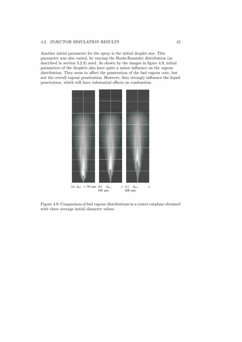
4.2. INJECTOR SIMULATION RESULTS 45
Another initial parameter for the spray is the initial droplet size. Thisparameter was also varied, by varying the Rosin-Rammler distribution (asdescribed in section 3.2.3) used. As shown by the images in figure 4.9, initialparameters of the droplets also have quite a minor influence on the vapourdistribution. They seem to affect the penetration of the fuel vapour core, butnot the overall vapour penetration. However, they strongly influence the liquidpenetration, which will have substantial effects on combustion.
(a) dav. = 50 µm (b) dav. =100 µm
(c) dav. =200 µm
Figure 4.9: Comparison of fuel vapour distributions in a centre cutplane obtainedwith three average initial diameter values
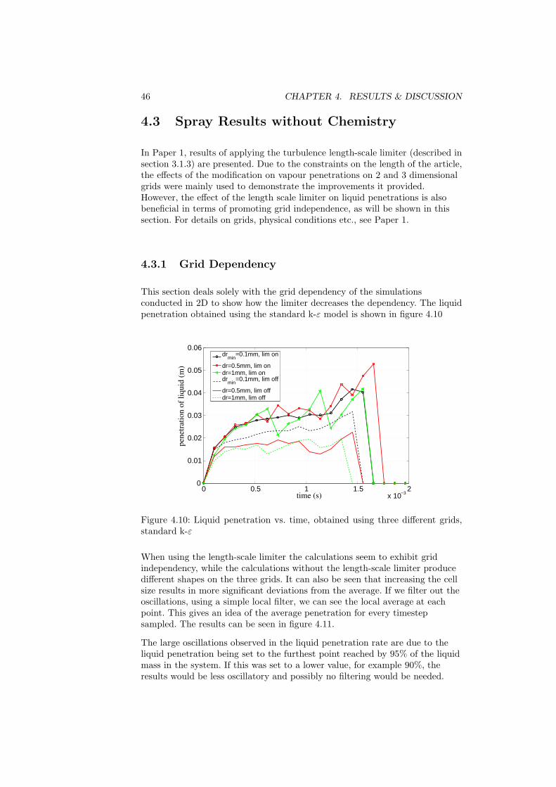
46 CHAPTER 4. RESULTS & DISCUSSION
4.3 Spray Results without Chemistry
In Paper 1, results of applying the turbulence length-scale limiter (described insection 3.1.3) are presented. Due to the constraints on the length of the article,the effects of the modification on vapour penetrations on 2 and 3 dimensionalgrids were mainly used to demonstrate the improvements it provided.However, the effect of the length scale limiter on liquid penetrations is alsobeneficial in terms of promoting grid independence, as will be shown in thissection. For details on grids, physical conditions etc., see Paper 1.
4.3.1 Grid Dependency
This section deals solely with the grid dependency of the simulationsconducted in 2D to show how the limiter decreases the dependency. The liquidpenetration obtained using the standard k-ε model is shown in figure 4.10
0 0.5 1 1.5 2x 10⁻³
0
0.01
0.02
0.03
0.04
0.05
0.06
time (s)
pene
tratio
n of
liqu
id (m
)
drmin
=0.1mm, lim on
dr=0.5mm, lim ondr=1mm, lim ondr
min=0.1mm, lim off
dr=0.5mm, lim offdr=1mm, lim off
Figure 4.10: Liquid penetration vs. time, obtained using three different grids,standard k-ε
When using the length-scale limiter the calculations seem to exhibit gridindependency, while the calculations without the length-scale limiter producedifferent shapes on the three grids. It can also be seen that increasing the cellsize results in more significant deviations from the average. If we filter out theoscillations, using a simple local filter, we can see the local average at eachpoint. This gives an idea of the average penetration for every timestepsampled. The results can be seen in figure 4.11.
The large oscillations observed in the liquid penetration rate are due to theliquid penetration being set to the furthest point reached by 95% of the liquidmass in the system. If this was set to a lower value, for example 90%, theresults would be less oscillatory and possibly no filtering would be needed.
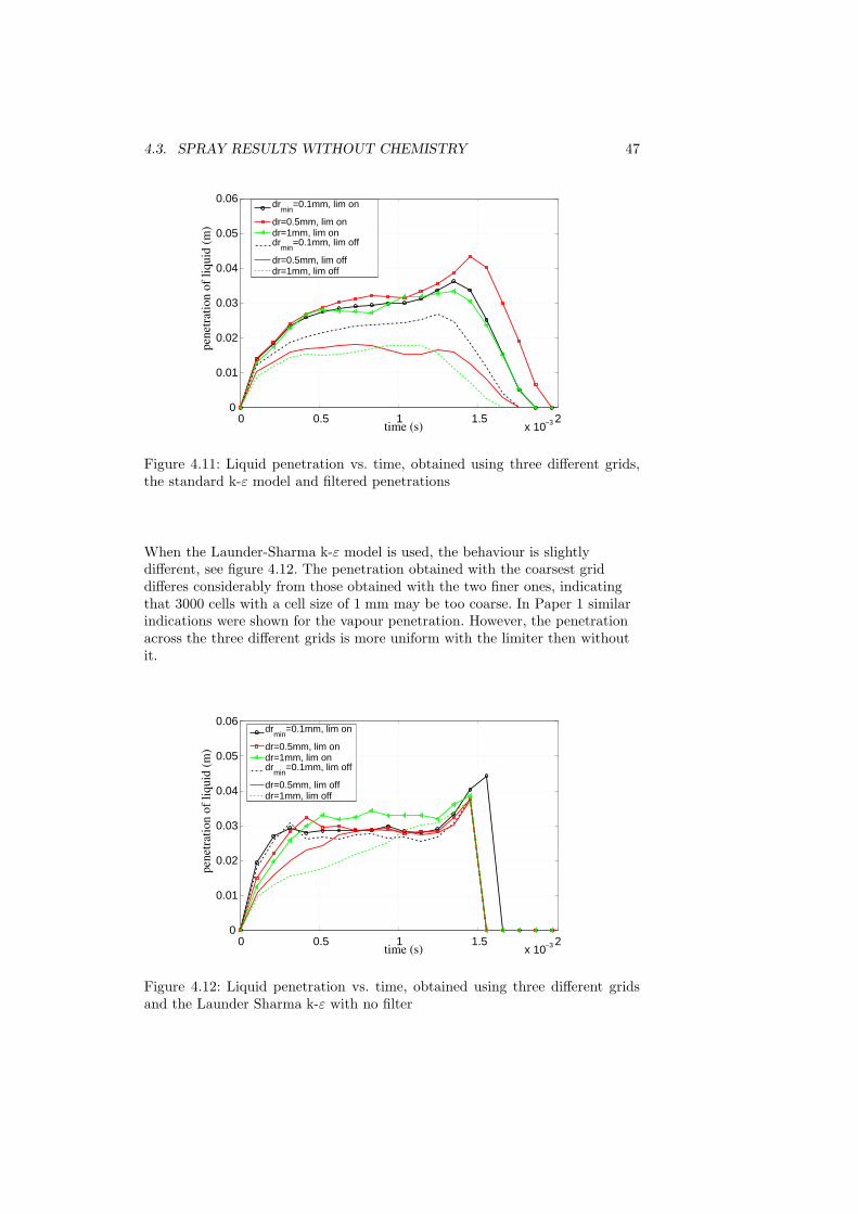
4.3. SPRAY RESULTS WITHOUT CHEMISTRY 47
0 0.5 1 1.5 2x 10⁻³
0
0.01
0.02
0.03
0.04
0.05
0.06
time (s)
pene
tratio
n of
liqu
id (m
)dr
min=0.1mm, lim on
dr=0.5mm, lim ondr=1mm, lim ondr
min=0.1mm, lim off
dr=0.5mm, lim offdr=1mm, lim off
Figure 4.11: Liquid penetration vs. time, obtained using three different grids,the standard k-ε model and filtered penetrations
When the Launder-Sharma k-ε model is used, the behaviour is slightlydifferent, see figure 4.12. The penetration obtained with the coarsest griddifferes considerably from those obtained with the two finer ones, indicatingthat 3000 cells with a cell size of 1 mm may be too coarse. In Paper 1 similarindications were shown for the vapour penetration. However, the penetrationacross the three different grids is more uniform with the limiter then withoutit.
0 0.5 1 1.5 2x 10⁻³
0
0.01
0.02
0.03
0.04
0.05
0.06
time (s)
pene
tratio
n of
liqu
id (m
)
drmin
=0.1mm, lim on
dr=0.5mm, lim ondr=1mm, lim ondr
min=0.1mm, lim off
dr=0.5mm, lim offdr=1mm, lim off
Figure 4.12: Liquid penetration vs. time, obtained using three different gridsand the Launder Sharma k-ε with no filter
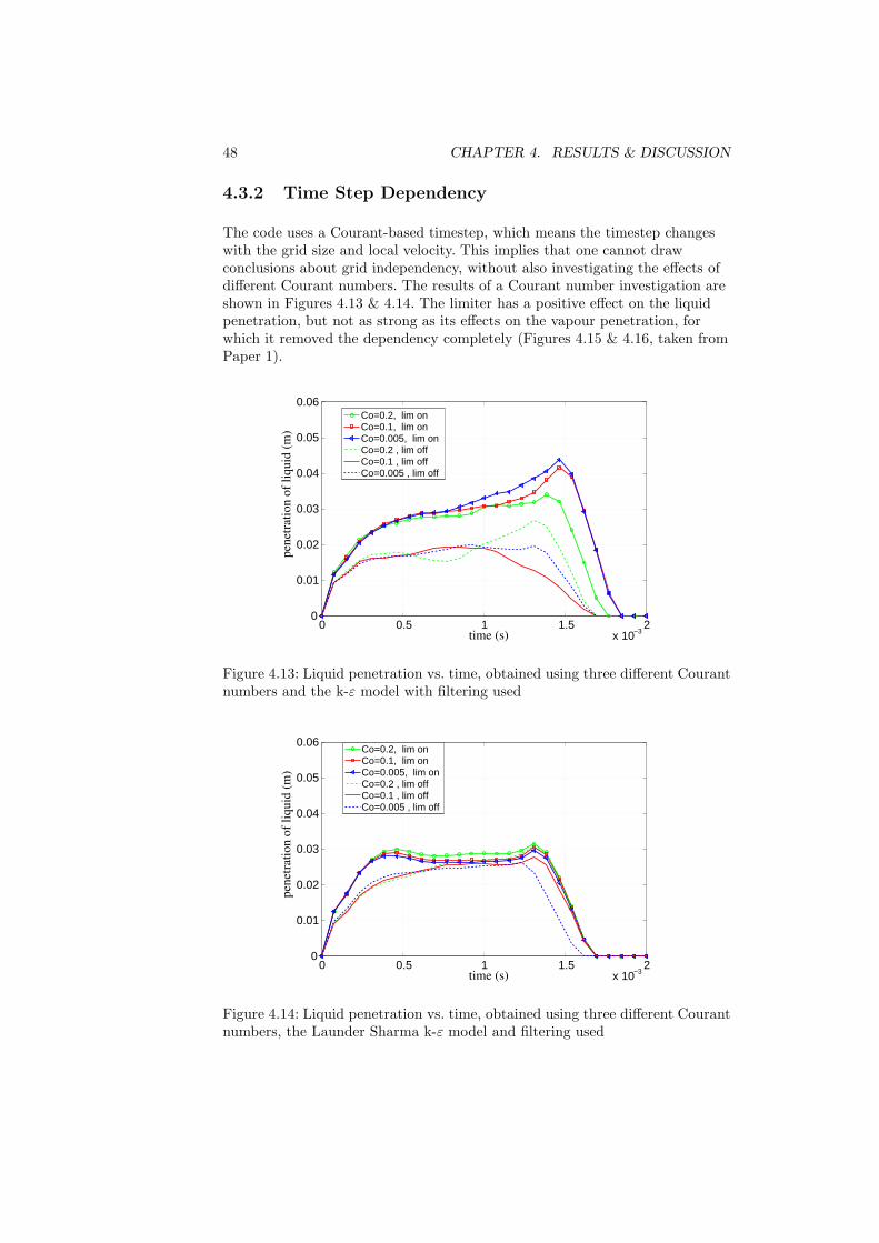
48 CHAPTER 4. RESULTS & DISCUSSION
4.3.2 Time Step Dependency
The code uses a Courant-based timestep, which means the timestep changeswith the grid size and local velocity. This implies that one cannot drawconclusions about grid independency, without also investigating the effects ofdifferent Courant numbers. The results of a Courant number investigation areshown in Figures 4.13 & 4.14. The limiter has a positive effect on the liquidpenetration, but not as strong as its effects on the vapour penetration, forwhich it removed the dependency completely (Figures 4.15 & 4.16, taken fromPaper 1).
0 0.5 1 1.5 2x 10⁻³
0
0.01
0.02
0.03
0.04
0.05
0.06
time (s)
pene
tratio
n of
liqu
id (m
)
Co=0.2, lim onCo=0.1, lim onCo=0.005, lim onCo=0.2 , lim offCo=0.1 , lim offCo=0.005 , lim off
Figure 4.13: Liquid penetration vs. time, obtained using three different Courantnumbers and the k-ε model with filtering used
0 0.5 1 1.5 2x 10⁻³
0
0.01
0.02
0.03
0.04
0.05
0.06
time (s)
pene
tratio
n of
liqu
id (m
)
Co=0.2, lim onCo=0.1, lim onCo=0.005, lim onCo=0.2 , lim offCo=0.1 , lim offCo=0.005 , lim off
Figure 4.14: Liquid penetration vs. time, obtained using three different Courantnumbers, the Launder Sharma k-ε model and filtering used
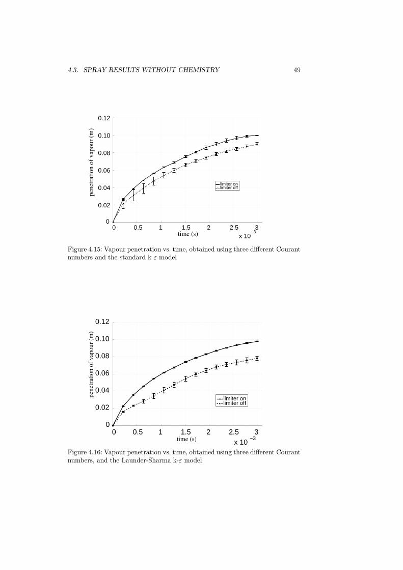
4.3. SPRAY RESULTS WITHOUT CHEMISTRY 49
0 0.5 1 1.5 2 2.5 3x 10
−3
0
0.02
0.04
0.06
0.08
0.10
0.12
time (s)
pene
tratio
n of
vap
our (
m)
limiter onlimiter off
Figure 4.15: Vapour penetration vs. time, obtained using three different Courantnumbers and the standard k-ε model
0 0.5 1 1.5 2 2.5 3x 10
−3
0
0.02
0.04
0.06
0.08
0.10
0.12
time (s)
pene
tratio
n of
vap
our (
m)
limiter onlimiter off
Figure 4.16: Vapour penetration vs. time, obtained using three different Courantnumbers, and the Launder-Sharma k-ε model
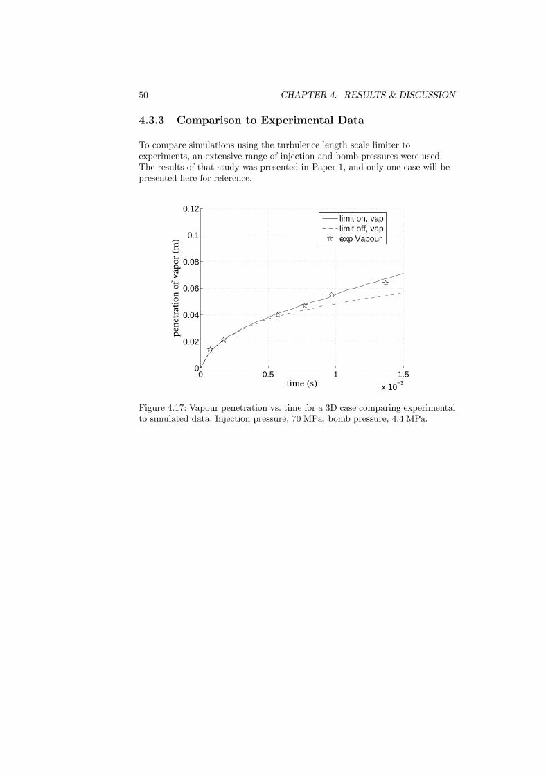
50 CHAPTER 4. RESULTS & DISCUSSION
4.3.3 Comparison to Experimental Data
To compare simulations using the turbulence length scale limiter toexperiments, an extensive range of injection and bomb pressures were used.The results of that study was presented in Paper 1, and only one case will bepresented here for reference.
0 0.5 1 1.5
x 10−3
0
0.02
0.04
0.06
0.08
0.1
0.12
time (s)
pene
tratio
n of
vap
or (m
)
limit on, vaplimit off, vapexp Vapour
Figure 4.17: Vapour penetration vs. time for a 3D case comparing experimentalto simulated data. Injection pressure, 70 MPa; bomb pressure, 4.4 MPa.
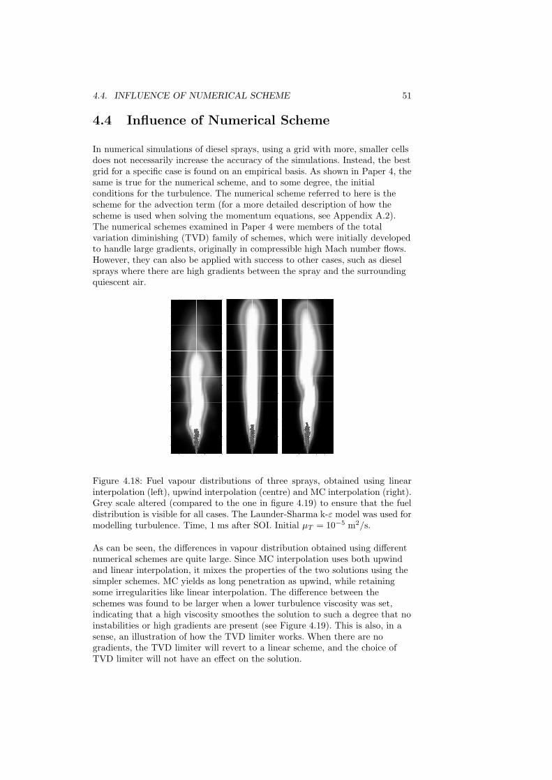
4.4. INFLUENCE OF NUMERICAL SCHEME 51
4.4 Influence of Numerical Scheme
In numerical simulations of diesel sprays, using a grid with more, smaller cellsdoes not necessarily increase the accuracy of the simulations. Instead, the bestgrid for a specific case is found on an empirical basis. As shown in Paper 4, thesame is true for the numerical scheme, and to some degree, the initialconditions for the turbulence. The numerical scheme referred to here is thescheme for the advection term (for a more detailed description of how thescheme is used when solving the momentum equations, see Appendix A.2).The numerical schemes examined in Paper 4 were members of the totalvariation diminishing (TVD) family of schemes, which were initially developedto handle large gradients, originally in compressible high Mach number flows.However, they can also be applied with success to other cases, such as dieselsprays where there are high gradients between the spray and the surroundingquiescent air.
Figure 4.18: Fuel vapour distributions of three sprays, obtained using linearinterpolation (left), upwind interpolation (centre) and MC interpolation (right).Grey scale altered (compared to the one in figure 4.19) to ensure that the fueldistribution is visible for all cases. The Launder-Sharma k-ε model was used formodelling turbulence. Time, 1 ms after SOI. Initial µT = 10−5 m2/s.
As can be seen, the differences in vapour distribution obtained using differentnumerical schemes are quite large. Since MC interpolation uses both upwindand linear interpolation, it mixes the properties of the two solutions using thesimpler schemes. MC yields as long penetration as upwind, while retainingsome irregularities like linear interpolation. The difference between theschemes was found to be larger when a lower turbulence viscosity was set,indicating that a high viscosity smoothes the solution to such a degree that noinstabilities or high gradients are present (see Figure 4.19). This is also, in asense, an illustration of how the TVD limiter works. When there are nogradients, the TVD limiter will revert to a linear scheme, and the choice ofTVD limiter will not have an effect on the solution.
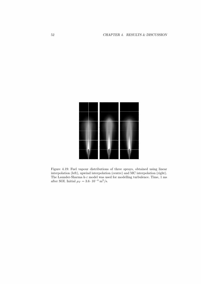
52 CHAPTER 4. RESULTS & DISCUSSION
Figure 4.19: Fuel vapour distributions of three sprays, obtained using linearinterpolation (left), upwind interpolation (centre) and MC interpolation (right).The Launder-Sharma k-ε model was used for modelling turbulence. Time, 1 msafter SOI. Initial µT = 3.6 · 10−4 m2/s.
4.5. FUEL SPRAYS WITH CHEMISTRY 53
4.5 Fuel Sprays with Chemistry
In Paper 3, simulations of events in the Sandia [73] constant-volume-vesselwere presented. The focus was on differences between KIVA-3V andOpenFOAM predictions of ignition delay time and flame lift-off length, andhow well the codes could calculate these parameters compared to experimentaldata. The simulations were performed on a cubic mesh with 108 mm sides forthe following conditions: ambient gas oxygen concentrations, 8-21 %; ambientgas temperatures, 750-1300 K; and ambient gas density, 14.8 kg/m3. Theinjector orifice diameter was 100 µm, and the injection pressure difference wasset to 1500 bar.
As can be seen from figures 4.20 through 4.23, OpenFOAM can predict theignition delay time and its dependence on ambient temperature and ambientoxygen concentration fairly well. This indicates of that the initial evaporationand chemical kinetics are “correct”. Unfortunately, the flame lift-off lengthpredictions are not as good. OpenFOAM seems to overpredict the changes inlift-off length caused by variations oxygen concentrations and ambienttemperature. KIVA-3V calculations use a set atomization length, as can beseen from figure 4.20, where the lift-off length is stable above 1100 K.OpenFOAM’s lift-off length is also stable for these temperatures, but this isbecause the flame cannot be any closer to the wall (due to the constanttemperature condition set along the walls).
The time sequence in figure 4.24 displays how the ignition starts and flamepropagates in OpenFOAM, KIVA-3V and experiments. The flame inOpenFOAM and KIVA-3V differs in two main respects. In OpenFOAM (andthe experiments) the flame ignites and then propagates upstream towards theinjector, whereas in KIVA-3V the flame ignites closer to the injector and thenthe flame lift-off length propagates downstream. The second main difference isthat OpenFOAM’s flame is very long and thin compared to KIVA-3V’s wider,shorter flame. The long flame generated by OpenFOAM penetrates much toofar, according to the experimental data. In the simulations Paper 4 is basedupon, this was found to be due to the numerical scheme and turbulence modelchosen. RNG k-ε is the k-ε turbulence model in OpenFOAM that produces thelongest flames, and the limited linear scheme in OpenFOAM was found topromote long, thin flames and fuel distributions. These results, and thequantitative results in figures 4.20-4.23 are extracted from Paper 3.
The computational time was much higher in OpenFOAM compared toKIVA-3V. The case with 21% oxygen took up to 70 hours on 4 processorsusing OpenFOAM, about 4 times the computational time for KIVA-3V. Themain reason for the high computational time is solving the chemical reactionrate equations. In OpenFOAM they are solved fully coupled using the SIBSODE solver as described in section 3.1.4. If the ODE solver for the chemistrycan be optimized to reduce the computational time without losing accuracy isan object for future work.
In addition to the two codes differing in computational time, there arenumerous other differences in the solver in two codes. OpenFOAM uses a
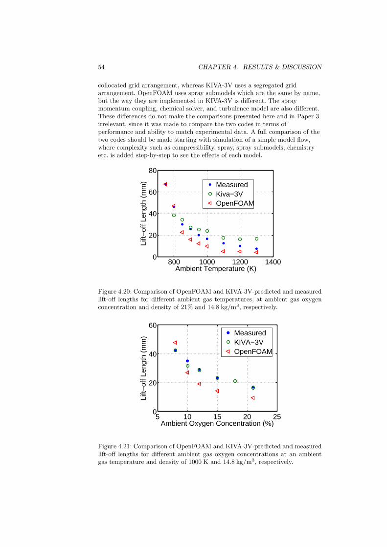
54 CHAPTER 4. RESULTS & DISCUSSION
collocated grid arrangement, whereas KIVA-3V uses a segregated gridarrangement. OpenFOAM uses spray submodels which are the same by name,but the way they are implemented in KIVA-3V is different. The spraymomentum coupling, chemical solver, and turbulence model are also different.These differences do not make the comparisons presented here and in Paper 3irrelevant, since it was made to compare the two codes in terms ofperformance and ability to match experimental data. A full comparison of thetwo codes should be made starting with simulation of a simple model flow,where complexity such as compressibility, spray, spray submodels, chemistryetc. is added step-by-step to see the effects of each model.
800 1000 1200 14000
20
40
60
80
Ambient Temperature (K)
Lift−
off L
engt
h (m
m)
MeasuredKiva−3VOpenFOAM
Figure 4.20: Comparison of OpenFOAM and KIVA-3V-predicted and measuredlift-off lengths for different ambient gas temperatures, at ambient gas oxygenconcentration and density of 21% and 14.8 kg/m3, respectively.
5 10 15 20 250
20
40
60
Ambient Oxygen Concentration (%)
Lift−
off L
engt
h (m
m)
MeasuredKIVA−3VOpenFOAM
Figure 4.21: Comparison of OpenFOAM and KIVA-3V-predicted and measuredlift-off lengths for different ambient gas oxygen concentrations at an ambientgas temperature and density of 1000 K and 14.8 kg/m3, respectively.
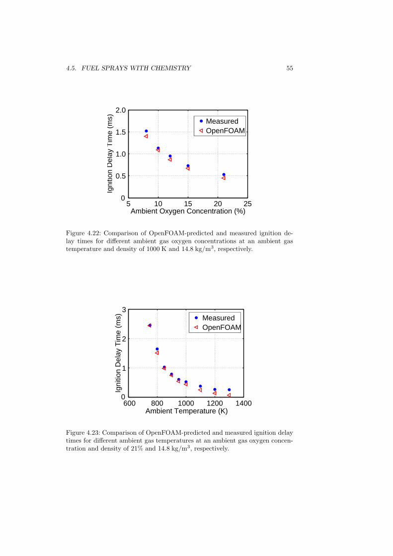
4.5. FUEL SPRAYS WITH CHEMISTRY 55
5 10 15 20 250
0.5
1.0
1.5
2.0
Ambient Oxygen Concentration (%)
Igni
tion
Del
ay T
ime
(ms)
MeasuredOpenFOAM
Figure 4.22: Comparison of OpenFOAM-predicted and measured ignition de-lay times for different ambient gas oxygen concentrations at an ambient gastemperature and density of 1000 K and 14.8 kg/m3, respectively.
600 800 1000 1200 14000
1
2
3
Ambient Temperature (K)
Igni
tion
Del
ay T
ime
(ms)
MeasuredOpenFOAM
Figure 4.23: Comparison of OpenFOAM-predicted and measured ignition delaytimes for different ambient gas temperatures at an ambient gas oxygen concen-tration and density of 21% and 14.8 kg/m3, respectively.
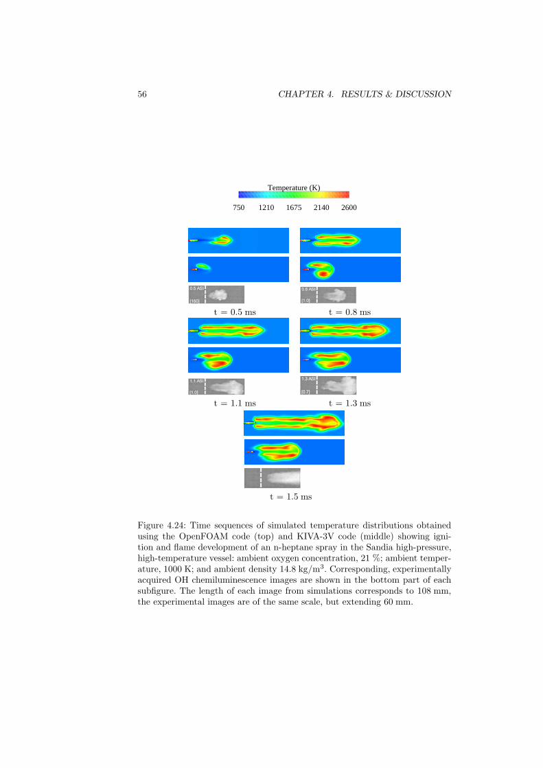
56 CHAPTER 4. RESULTS & DISCUSSION
750 1210 1675 2140 2600
Temperature (K)
PSfrag replacements
Temperature
PSfrag replacementsTemperature
PSfrag replacementsTemperature
PSfrag replacementsTemperature
PSfrag replacementsTemperature
PSfrag replacementsTemperature
PSfrag replacementsTemperature
t = 0.5 ms t = 0.8 ms
PSfrag replacementsTemperature
PSfrag replacementsTemperature
PSfrag replacementsTemperature
PSfrag replacementsTemperature
PSfrag replacementsTemperature
PSfrag replacementsTemperature
t = 1.1 ms t = 1.3 ms
PSfrag replacementsTemperature
PSfrag replacementsTemperature
PSfrag replacementsTemperature
t = 1.5 ms
Figure 4.24: Time sequences of simulated temperature distributions obtainedusing the OpenFOAM code (top) and KIVA-3V code (middle) showing igni-tion and flame development of an n-heptane spray in the Sandia high-pressure,high-temperature vessel: ambient oxygen concentration, 21 %; ambient temper-ature, 1000 K; and ambient density 14.8 kg/m3. Corresponding, experimentallyacquired OH chemiluminescence images are shown in the bottom part of eachsubfigure. The length of each image from simulations corresponds to 108 mm,the experimental images are of the same scale, but extending 60 mm.
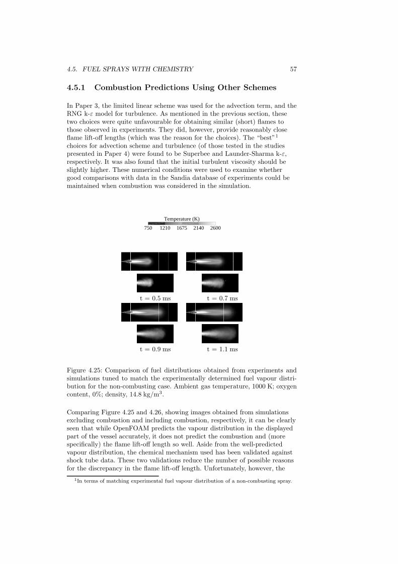
4.5. FUEL SPRAYS WITH CHEMISTRY 57
4.5.1 Combustion Predictions Using Other Schemes
In Paper 3, the limited linear scheme was used for the advection term, and theRNG k-ε model for turbulence. As mentioned in the previous section, thesetwo choices were quite unfavourable for obtaining similar (short) flames tothose observed in experiments. They did, however, provide reasonably closeflame lift-off lengths (which was the reason for the choices). The “best”1
choices for advection scheme and turbulence (of those tested in the studiespresented in Paper 4) were found to be Superbee and Launder-Sharma k-ε,respectively. It was also found that the initial turbulent viscosity should beslightly higher. These numerical conditions were used to examine whethergood comparisons with data in the Sandia database of experiments could bemaintained when combustion was considered in the simulation.
750 1210 1675 2140 2600
Temperature (K)
t = 0.5 ms t = 0.7 ms
t = 0.9 ms t = 1.1 ms
Figure 4.25: Comparison of fuel distributions obtained from experiments andsimulations tuned to match the experimentally determined fuel vapour distri-bution for the non-combusting case. Ambient gas temperature, 1000 K; oxygencontent, 0%; density, 14.8 kg/m3.
Comparing Figure 4.25 and 4.26, showing images obtained from simulationsexcluding combustion and including combustion, respectively, it can be clearlyseen that while OpenFOAM predicts the vapour distribution in the displayedpart of the vessel accurately, it does not predict the combustion and (morespecifically) the flame lift-off length so well. Aside from the well-predictedvapour distribution, the chemical mechanism used has been validated againstshock tube data. These two validations reduce the number of possible reasonsfor the discrepancy in the flame lift-off length. Unfortunately, however, the
1In terms of matching experimental fuel vapour distribution of a non-combusting spray.
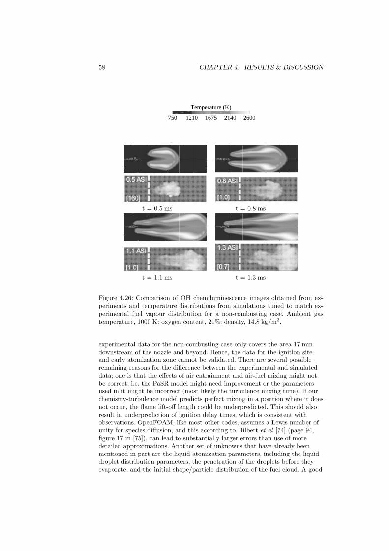
58 CHAPTER 4. RESULTS & DISCUSSION
750 1210 1675 2140 2600
Temperature (K)
t = 0.5 ms t = 0.8 ms
t = 1.1 ms t = 1.3 ms
Figure 4.26: Comparison of OH chemiluminescence images obtained from ex-periments and temperature distributions from simulations tuned to match ex-perimental fuel vapour distribution for a non-combusting case. Ambient gastemperature, 1000 K; oxygen content, 21%; density, 14.8 kg/m3.
experimental data for the non-combusting case only covers the area 17 mmdownstream of the nozzle and beyond. Hence, the data for the ignition siteand early atomization zone cannot be validated. There are several possibleremaining reasons for the difference between the experimental and simulateddata; one is that the effects of air entrainment and air-fuel mixing might notbe correct, i.e. the PaSR model might need improvement or the parametersused in it might be incorrect (most likely the turbulence mixing time). If ourchemistry-turbulence model predicts perfect mixing in a position where it doesnot occur, the flame lift-off length could be underpredicted. This should alsoresult in underprediction of ignition delay times, which is consistent withobservations. OpenFOAM, like most other codes, assumes a Lewis number ofunity for species diffusion, and this according to Hilbert et al [74] (page 94,figure 17 in [75]), can lead to substantially larger errors than use of moredetailed approximations. Another set of unknowns that have already beenmentioned in part are the liquid atomization parameters, including the liquiddroplet distribution parameters, the penetration of the droplets before theyevaporate, and the initial shape/particle distribution of the fuel cloud. A good
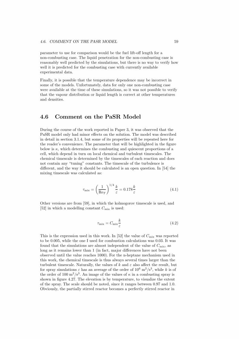
4.6. COMMENT ON THE PASR MODEL 59
parameter to use for comparison would be the fuel lift-off length for anon-combusting case. The liquid penetration for the non-combusting case isreasonably well predicted by the simulations, but there is no way to verify howwell it is predicted for the combusting case with currently availableexperimental data.
Finally, it is possible that the temperature dependence may be incorrect insome of the models. Unfortunately, data for only one non-combusting casewere available at the time of these simulations, so it was not possible to verifythat the vapour distribution or liquid length is correct at other temperaturesand densities.
4.6 Comment on the PaSR Model
During the course of the work reported in Paper 3, it was observed that thePaSR model only had minor effects on the solution. The model was describedin detail in section 3.1.4, but some of its properties will be repeated here forthe reader’s convenience. The parameter that will be highlighted in the figurebelow is κ, which determines the combusting and quiescent proportions of acell, which depend in turn on local chemical and turbulent timescales. Thechemical timescale is determined by the timescales of each reaction and doesnot contain any “tuning” constants. The timescale of the turbulence isdifferent, and the way it should be calculated is an open question. In [54] themixing timescale was calculated as:
τmix =
(1
ReT
)1/4k
ε= 0.178
k
ε(4.1)
Other versions are from [59], in which the kolmogorov timescale is used, and[52] in which a modelling constant Cmix is used:
τmix = Cmixk
ε(4.2)
This is the expression used in this work. In [52] the value of Cmix was reportedto be 0.005, while the one I used for combustion calculations was 0.03. It wasfound that the simulations are almost independent of the value of Cmix, aslong as it remains lower than 1 (in fact, major differences have not beenobserved until the value reaches 1000). For the n-heptane mechanism used inthis work, the chemical timescale is thus always several times larger than theturbulent timescale. Naturally, the values of k and ε also affect the result, butfor spray simulations ε has an average of the order of 106 m2/s3, while k is ofthe order of 100 m2/s3. An image of the values of κ in a combusting spray isshown in figure 4.27. The elevation is by temperature, to visualize the extentof the spray. The scale should be noted, since it ranges between 0.97 and 1.0.Obviously, the partially stirred reactor becomes a perfectly stirred reactor in
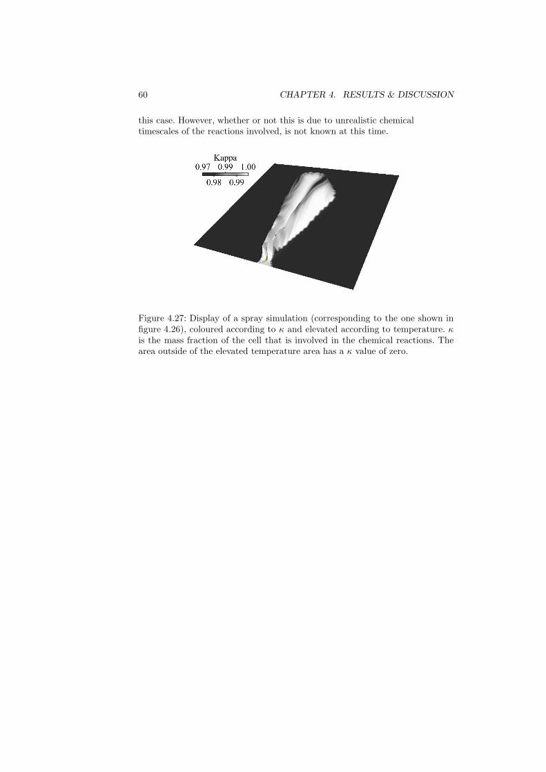
60 CHAPTER 4. RESULTS & DISCUSSION
this case. However, whether or not this is due to unrealistic chemicaltimescales of the reactions involved, is not known at this time.
Figure 4.27: Display of a spray simulation (corresponding to the one shown infigure 4.26), coloured according to κ and elevated according to temperature. κis the mass fraction of the cell that is involved in the chemical reactions. Thearea outside of the elevated temperature area has a κ value of zero.
Chapter 5
Conclusions
A code describing how a fluid cavitates when it is subjected to low pressuresdue to geometric contraction was successfully used to simulate data acquiredfrom model nozzle experiments performed at AVL. The thesis shows that thereare many pitfalls on the way to simulations that provide good comparisons toexperimental events, as well as presenting some final results from the study.Examples of the degree of influence the injection model can have over theEuler-Lagrangian spray simulations are also presented, together with anexample of results obtained using the three-phase code (mainly for illustrativepurposes since this code has not been validated). These simulations were, asstated in the outline of the thesis (section 1.4), intended to be used for thedevelopment of an injection/atomization model for Euler-Lagrangian dieselspray simulations. Unfortunately, due to the high complexity of the problem,no such model could be developed. For a more detailed description of theencountered problems when simulating cavitating diesel injections, see section4.1.
Regarding spray grid and time-step independence, the results from Paper 1and section 4.3 clearly show that dependence diminishes when a limiter on thelength scale of the turbulence is applied. The importance of this result cannotbe over-emphasised, since shorter computational time means moreinvestigations can be made, or results can be obtained in a shorter time. Inshort, it improves the efficiency of the CFD modelling.
The results also show how flame lift-off length and ignition delay time can bepredicted by OpenFOAM, and the effects of varying the ambient oxygenconcentrations and temperatures on these parameters. OpenFOAM was foundto perform well when predicting the propagation of the flame compared to theignition site, and in ignition delay time. However, it was found to underpredictthe flame lift-off length and its dependency on temperature and ambientoxygen concentration. For a non-combusting case in the same geometry,OpenFOAM could predict the vapour distribution very well, in addition to theliquid and vapour penetration lengths.
61
62 CHAPTER 5. CONCLUSIONS
To further analyze the reason for the short flame lift-off lengths yielded byOpenFOAM, the calculations and results of Siebers et al [76] were used. Thecited report describes a way to estimate the percentage of stoichiometric airentrained (ξ) upstream of the lift-off length. According to this estimate, thepercentage of entrained air is 29% of the air required for stoichiometriccombustion, which is consistent with the article’s relationship betweeninjection velocity and ξ. Furthermore, according to the report, the liquiddroplets and flame should be separated in distance much more from theinjector than they are in figure 4.26. If the turbulence/chemistry interactionmodel used required more air to be entrained before combustion, the flamelift-off length might be increased without increasing the length of the flame.As indicated in section 4.6, the PaSR model does not suffice for this task.
The choice of scheme can have a large influence on the fuel vapourdistribution, and thus on the resulting flame and combustion. This wasdemonstrated in paper 4, and also in sections 4.4 and 4.5.1. These effects areimportant to be aware of, in addition to the effects of numerical grid andturbulence model. In the work this thesis was based upon, the SuperBee TVDlimiter was found to give the best results compared to experiments, but thisfinding could be (like the choice of grid) problem-dependent.
Chapter 6
Future Work
As shown in this thesis, diesel spray simulations using the Euler-Lagrangianapproach are helpful, but they are not yet predictive. Therefore, much workneeds to be done to improve them. Briefly, two possible approaches could beadopted in attempts to improve diesel spray simulations: Euler-Euler typesimulations, which have only been used for primary breakup studies to date; ormore sophisticated Euler-Lagrangian descriptions. Following the secondapproach, implies use of LES to model gas phase turbulence and bettersub-models for the liquid-gas interactions. Another option is the VSB2 spraymodel developed by Karlsson [77], in which the Lagrangian parcels/blobs donot interact with the grid directly, but through bubbles of varying size.Furthermore, the Lagrangian parcels contain a distribution of blobs instead ofequally sized droplets. Details of this setup are not known at this time, butmight be published in the future.
In the nearer future, possible areas of future work are to continue effortsstarted in the studies published in Papers 3 and 4. As shown in the Resultssection, while the models presented in Paper 4 delivered fuel vapourdistributions that approximated well to experimentally observed distributions,the resulting flames were not well predicted when chemistry was considered.Since we can now assume that the spray and vapour distributions are welltuned, the parts of the code that are largely responsible for the errors must bethe turbulence/chemistry interaction (PaSR model), temperature dependencyof the liquid penetration, primary breakup and initial vapour cloud formation,or the chemical mechanism itself. However, the chemical mechanism has beenverified against shock-tube experiments, and seems to produce goodcomparisons for those cases. A way to rule out temperature dependency wouldbe to run simulations and compare them to the results of correspondingexperiments, without oxygen using different ambient temperatures. Thevalidation presented in Paper 3 is only against one case, due to a lack of datafrom non-combusting experiments with well-defined boundary conditions tocompare to the simulations.
63
64 CHAPTER 6. FUTURE WORK
When the results presented in Paper 3 are to be improved (beyond theimprovement presented in this thesis), a large number of simulations where thechemical reactions are considered will have to be run. It would then bedesirable to have optimized the solver for the chemical mechanism, as thecomputational time occupied by the solver in OpenFOAM is currently veryhigh (as mentioned in section 4.5).
It would also be interesting to venture further down the path taken in Paper 2,investigating in detail how the initial droplet parameters influence the sprayand combustion. The most important of these parameters, based on the shortpreliminary study, seems to be the initial droplet size distribution. It is likelythat a good atomization and injection model would improve the flame lift-offlength predictions presented in Paper 3, since the liquid penetration length hasa strong influence on the ignition point and its propagation. These twoapproaches are linked in the sense that they both are concerned with theprimary events of spray development. Simulating cavitating diesel flowrequires a more robust model than the one used in Paper 2, and perhaps it isnot even essential to the development of a new injection model. There arestudies ([78, 79]) which links injection pressure, nozzle diameter, to sprayangle, discharge coefficient etc. If these studies were used like the cavitationsimulations were intended to be used, a diesel injection model could bedeveloped based on experimental studies instead of numerical simulations.
Other aspects not covered in the thesis could be of interest for future work.One such aspect is the obvious extension from constant volume vesselsimulations to engine simulations. OpenFOAM has the functionality to handlemoving meshes with valves and other topological changes [80], so using thework described in Papers 3 and 4 as a basis for engine simulations to explorethe effects of key variables in engines could be of high value to both the enginecommunity and the numerical community.
Aside from using k-ε models and LES it could also be useful to assess thepossible utility of other turbulence models such as k-ω type models, unsteadyRANS models or other hybrid type turbulence models. It is possible that theturbulence plays a major role in obtaining correct air entrainment formodelling the early spray development and flame lift-off lengths.
6.1 Outlook
As mentioned above, it would be helpful to have access to an experimentaldatabase covering a larger array of non-combusting cases than the single casefrom Sandia. It would also be beneficial for research in numerical methods tohave more data on the initial breakup of sprays for both combusting andnon-combusting cases. A good example of a study that presented relevantdata, in this respect, is one by Ochoterena et al [81], in which both liquid andvapour penetration lengths are presented along with flame lift-off lengths, coneangles and flame temperatures. Unfortunately, from a modeller’s perspective,the fuels used are not as easy to model as, for instance, n-heptane, and theexperiments were only run in combusting conditions. However, it should be
6.1. OUTLOOK 65
noted that supplying modellers with input for simulations was not one of thestated objectives of the cited study ([81]).
In light of the increasing need for more experimental data specifically tailoredfor validating numerical simulations, the author belives and stronglyrecommends that more experiments tailored for numerical simulations shouldbe performed. Close, long-term co-operation between a modeller and anempirical investigator with access to both spray chamber and engine equipmentwould have every chance of making major advances in spray modelling.Furthermore, the need for good spray modelling will probably increase asengine concepts become more advanced and new fuels are introduced, to helpensure that demands from customers and legislation are met.
Finally, we return to the starting point of the thesis; horses in early 20thcentury America. During this period, commuters were facing rising prices forhay and oats, as well as increased public fears about pollution and traffic jams[1]. This situation is uncomfortably similar to current circumstances.Hopefully, the solution we devise this time will not lead to the same problems100 years from now.

66 CHAPTER 6. FUTURE WORK
Chapter 7
Summary of Papers
The thesis is based on the work published in the following papers
Paper I - Numerical Investigation ofMesh/Turbulence/Spray Interaction for Diesel
Applications
This paper originated from attempts to solve the problem of grid dependencedescribed in section 1.4. The solution was based on a suggestion in the book“Modeling Engine Spray and Combustion Processes” by Gunnar Stiesch [12],p.183, that the turbulence length scale should be limited to the jet diameterwithin the jet region. The rationale for this is that the jet is the driving forcefor the turbulence in spray simulations. This was implemented in theOpenFOAM code, and tested on different sized grids in 2D and 3D, as well asusing different time-steps. It was shown in the article that the length scalelimiter was very beneficial in terms of reducing grid and time-step dependency.The results were also compared to data acquired in experiments performed atChalmers on fuel injection into a high-pressure, high-temperature constantvolume vessel. The multi-component model diesel fuel IDEA was used as thefuel. The simulations using the turbulence length scale limiter proved toprovide better matches to the experimental data than when it was turned off.The most important finding was that the grid and time step dependency couldbe reduced by introducing the length scale limiter.
The simulations and paper were planned together with Dr Niklas Nordin, whoalso implemented the limiter in the code. I was responsible for the preliminarystudies that were not included in the paper, to determine limiter size, gridoptimization etc. I was also responsible for running and post-processing all butone of the simulations included in the paper, the remaining one was performedby Dr Niklas Nordin. The experimental data used were acquired by Alf-HugoMagnusson at Chalmers University of Technology. The paper was written by
67
68 CHAPTER 7. SUMMARY OF PAPERS
me, together with Dr Niklas Nordin, and I presented it at the SAE Fuel andLubricants Conference, 2005, in Rio de Janeiro, Brazil.
Paper II - Modelling Injector Flow Including
Cavitation Effects for Diesel Applications
This paper was preceded by several attempts to model diesel injector flow.The initial intention was to develop and present a new injection model,together with validation of the code for the injector flow, in the same article.However, simulating injector flow proved to be much more complex thananticipated, so a decision was taken to focus solely on the validation in thispaper, while the injector model would be the topic of a possible later paper.The code used in this paper was written by OpenCFD Ltd., as a by-product ofa code to simulate diesel injector flow with the ambient air as well ascavitating diesel liquid.
I setup, ran and post-processed the simulations, with numerical help fromHenry Weller, who developed the code used. However, as these simulationsrequired extensive testing, I ran months of simulations, with various numericalsetups to ensure a stable solution, before the article was written. Theempirical data used for comparison were acquired from experiments performedat AVL. I wrote the paper with inputs from Dr Niklas Nordin and HenryWeller. In addition, I presented it at the 5th Joint ASME/JSME FluidsEngineering Conference, 2007, San Diego, USA.
Paper III - Three Dimensional Simulation ofDiesel Spray Ignition and Flame Lift-Off Using
OpenFOAM and KIVA-3V CFD Codes
The paper originated from a comparison of OpenFOAM results I generated toKIVA-3V results generated by Dr Feng Tao. Thanks to the large ECNdatabase, it was also possible to compare the results to experimental data. Wecompared the effects of varying amounts of oxygen/EGR and ambienttemperatures using the two codes. There was also a limited comparison of theeffects of using different grids and injection positions (published in theAppendix of the article). It was found that OpenFOAM produces much longerflames than KIVA-3V, as well as short flame lift-off lengths. It is possible thatKIVA-3V yields longer flame lift-off lengths since the atomization length isprescribed in the code. The OpenFOAM simulations did not use anatomization model, and thus yielded much shorter liquid penetrations.Unfortunate use of the RNG k-εturbulence model together with the limitedLinear scheme is believed to be an underlying reason for the long penetrationof the flame. With the knowledge gained from the studies published in PaperIV, I believe the results would have been better if SuperBee interpolation hadbeen used for the advection scheme.
69
I setup, ran and post-processed the OpenFOAM simulations, while theKIVA-3V simulations were setup, ran and post-processed by Dr Feng Tao. Thepaper was written by me and Dr Feng Tao. I presented it at the SAE WorldCongress, 2008, Detroit, USA.
Paper IV - Influence of Advection Schemes In
The Prediction of Diesel Spray and Fuel VapourDistributions
As mentioned regarding the previous paper, the authors were not satisfied byOpenFOAM’s overprediction of flame lengths. Simulations indicated that thescheme might have a strong influence on the fuel vapour distribution.Therefore, a more extensive study of the influence of the scheme (and effects ofthe initial parameters on spray development) was undertaken. It was foundthat while the scheme does have a large influence, the initial turbulenceparameters can reduce or enhance its influence. If the initial viscosity of theturbulence is low, the SuperBee scheme was shown to be the best choice forinterpolation of the advection scheme.
I setup, ran and post-procssed the simulations, and wrote the paper togetherwith Dr Feng Tao. It was presented at ILASS, 2008, Como Lake, Italy.

70 CHAPTER 7. SUMMARY OF PAPERS
Appendix A
Implementation inOpenFOAM
A.1 Rhie-Chow Interpolation in OpenFOAM
OpenFOAM is relatively new, open source code that is not fully documented.Therefore the intention of the author here is to extend the documentation, andat the same time share some additional knowledge that has been gained duringthe course of this work. One very important aspect of CFD is Rhie-Chowcorrection, which will therefore be described here. Rhie-Chow correction isabsolutely necessary for flow simulations using a collocated grid, since itremoves oscillations in the solution, which occur if the pressure gradient doesnot depend on the pressure in adjacent cells, thus allowing a “jigsaw” patternto develop.
Some basic information about the notation in OpenFOAM is needed todescribe how it works. Partial Differential Equations in OpenFOAM are solvedby setting up the appropriate matrix system:
fvm::operation(coefficient,U) (A.1)
This means that the solver is to solve for U, and coefficient is a coefficientwhich can vary in space and/or time, or be a constant. Operations like thiswill be described many times throughout this section, and it is important tounderstand the nomenclature. Further, this section contains two velocities: U,which is used for the flux and held constant when the momentum equationsare solved; and Ux,y,z, which is the velocity we solve for. All equationscontaining Ux,y,z are actually three equations, referring to relationships in thex-, y-, and z-direction respectively.
Rhie and Chow is usually regarded as a correction proportional to thedifference between the pressure gradient at the face and the interpolated
71
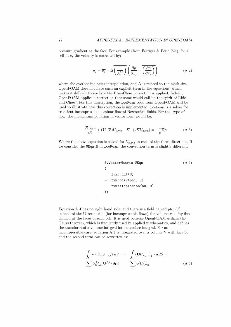
72 APPENDIX A. IMPLEMENTATION IN OPENFOAM
pressure gradient at the face. For example (from Ferziger & Peric [82]), for acell face, the velocity is corrected by:
uj = uj − ∆
(1
Aujp
)(
∂p
∂xj−(∂p
∂xj
))
(A.2)
where the overbar indicates interpolation, and ∆ is related to the mesh size.OpenFOAM does not have such an explicit term in the equations, whichmakes it difficult to see how the Rhie-Chow correction is applied. Indeed,OpenFOAM applies a correction that some would call ’in the spirit of Rhieand Chow’. For this description, the icoFoam code from OpenFOAM will beused to illustrate how this correction is implemented. icoFoam is a solver fortransient incompressible laminar flow of Newtonian fluids. For this type offlow, the momentum equation in vector form would be:
∂Ux,y,z
∂t+ (U · ∇)Ux,y,z −∇ · (ν∇Ux,y,z) = −1
ρ∇p (A.3)
Where the above equation is solved for Ux,y,z in each of the three directions. Ifwe consider the UEqn.H in icoFoam, the convection term is slightly different.
fvVectorMatrix UEqn (A.4)
(
fvm::ddt(U)
+ fvm::div(phi, U)
− fvm::laplacian(nu, U)
);
Equation A.4 has no right hand side, and there is a field named phi (φ)instead of the U-term. φ is (for incompressible flows) the volume velocity fluxdefined at the faces of each cell. It is used because OpenFOAM utilizes theGauss theorem, which is frequently used in applied mathematics, and definesthe transform of a volume integral into a surface integral. For anincompressible case, equation A.3 is integrated over a volume V with face S,and the second term can be rewritten as:
∫
V
∇ · (UUx,y,z) dV =
∫
S
(UUx,y,z)f · n dS =
=∑
i
Uf,ix,y,z(Uf,i ·Sf i) =
∑
i
φiUf,ix,y,z (A.5)
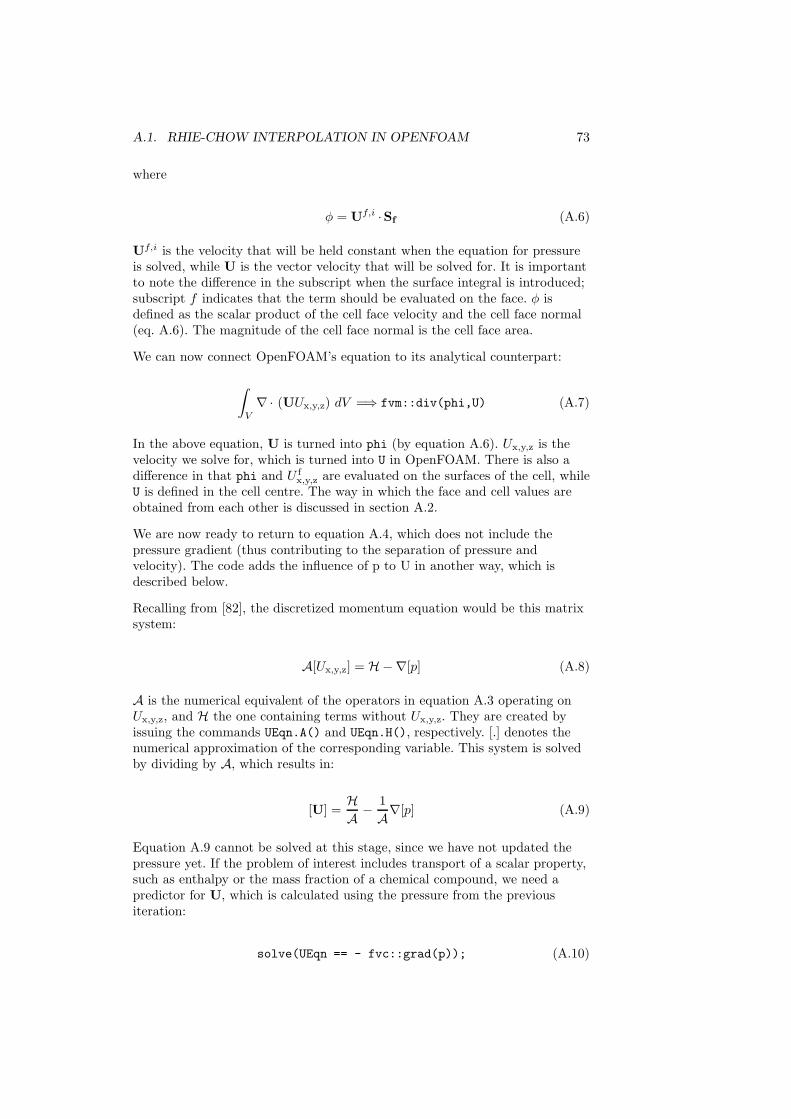
A.1. RHIE-CHOW INTERPOLATION IN OPENFOAM 73
where
φ = Uf,i ·Sf (A.6)
Uf,i is the velocity that will be held constant when the equation for pressureis solved, while U is the vector velocity that will be solved for. It is importantto note the difference in the subscript when the surface integral is introduced;subscript f indicates that the term should be evaluated on the face. φ isdefined as the scalar product of the cell face velocity and the cell face normal(eq. A.6). The magnitude of the cell face normal is the cell face area.
We can now connect OpenFOAM’s equation to its analytical counterpart:
∫
V
∇ · (UUx,y,z) dV =⇒ fvm::div(phi,U) (A.7)
In the above equation, U is turned into phi (by equation A.6). Ux,y,z is thevelocity we solve for, which is turned into U in OpenFOAM. There is also adifference in that phi and U f
x,y,z are evaluated on the surfaces of the cell, whileU is defined in the cell centre. The way in which the face and cell values areobtained from each other is discussed in section A.2.
We are now ready to return to equation A.4, which does not include thepressure gradient (thus contributing to the separation of pressure andvelocity). The code adds the influence of p to U in another way, which isdescribed below.
Recalling from [82], the discretized momentum equation would be this matrixsystem:
A[Ux,y,z] = H−∇[p] (A.8)
A is the numerical equivalent of the operators in equation A.3 operating onUx,y,z, and H the one containing terms without Ux,y,z. They are created byissuing the commands UEqn.A() and UEqn.H(), respectively. [.] denotes thenumerical approximation of the corresponding variable. This system is solvedby dividing by A, which results in:
[U] =HA − 1
A∇[p] (A.9)
Equation A.9 cannot be solved at this stage, since we have not updated thepressure yet. If the problem of interest includes transport of a scalar property,such as enthalpy or the mass fraction of a chemical compound, we need apredictor for U, which is calculated using the pressure from the previousiteration:
solve(UEqn == - fvc::grad(p)); (A.10)
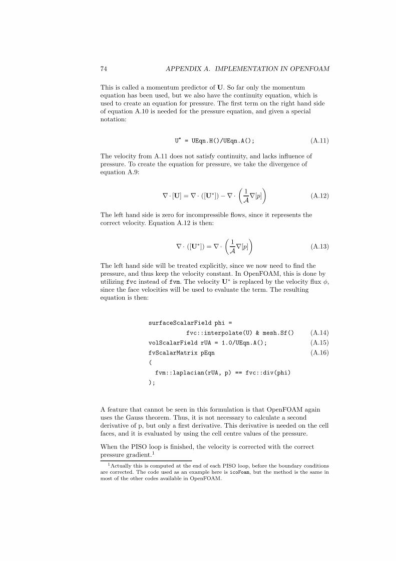
74 APPENDIX A. IMPLEMENTATION IN OPENFOAM
This is called a momentum predictor of U. So far only the momentumequation has been used, but we also have the continuity equation, which isused to create an equation for pressure. The first term on the right hand sideof equation A.10 is needed for the pressure equation, and given a specialnotation:
U* = UEqn.H()/UEqn.A(); (A.11)
The velocity from A.11 does not satisfy continuity, and lacks influence ofpressure. To create the equation for pressure, we take the divergence ofequation A.9:
∇ · [U] = ∇ · ([U∗]) −∇ ·(
1
A∇[p]
)
(A.12)
The left hand side is zero for incompressible flows, since it represents thecorrect velocity. Equation A.12 is then:
∇ · ([U∗]) = ∇ ·(
1
A∇[p]
)
(A.13)
The left hand side will be treated explicitly, since we now need to find thepressure, and thus keep the velocity constant. In OpenFOAM, this is done byutilizing fvc instead of fvm. The velocity U∗ is replaced by the velocity flux φ,since the face velocities will be used to evaluate the term. The resultingequation is then:
surfaceScalarField phi =
fvc::interpolate(U) & mesh.Sf() (A.14)
volScalarField rUA = 1.0/UEqn.A(); (A.15)
fvScalarMatrix pEqn (A.16)
(
fvm::laplacian(rUA, p) == fvc::div(phi)
);
A feature that cannot be seen in this formulation is that OpenFOAM againuses the Gauss theorem. Thus, it is not necessary to calculate a secondderivative of p, but only a first derivative. This derivative is needed on the cellfaces, and it is evaluated by using the cell centre values of the pressure.
When the PISO loop is finished, the velocity is corrected with the correctpressure gradient.1
1Actually this is computed at the end of each PISO loop, before the boundary conditionsare corrected. The code used as an example here is icoFoam, but the method is the same inmost of the other codes available in OpenFOAM.
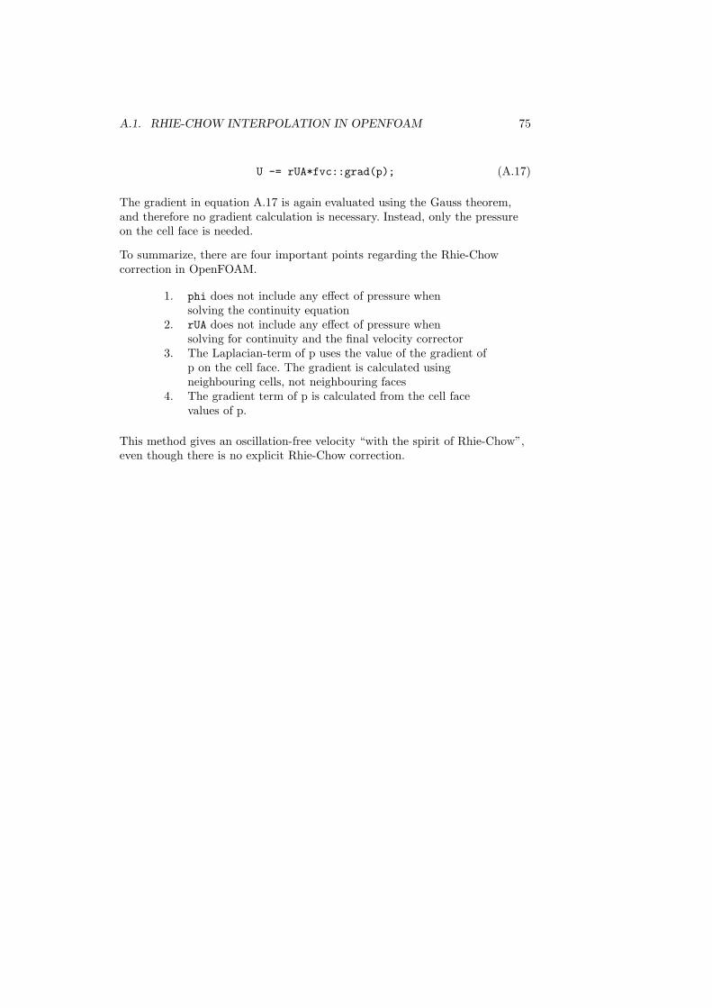
A.1. RHIE-CHOW INTERPOLATION IN OPENFOAM 75
U -= rUA*fvc::grad(p); (A.17)
The gradient in equation A.17 is again evaluated using the Gauss theorem,and therefore no gradient calculation is necessary. Instead, only the pressureon the cell face is needed.
To summarize, there are four important points regarding the Rhie-Chowcorrection in OpenFOAM.
1. phi does not include any effect of pressure whensolving the continuity equation
2. rUA does not include any effect of pressure whensolving for continuity and the final velocity corrector
3. The Laplacian-term of p uses the value of the gradient ofp on the cell face. The gradient is calculated usingneighbouring cells, not neighbouring faces
4. The gradient term of p is calculated from the cell facevalues of p.
This method gives an oscillation-free velocity “with the spirit of Rhie-Chow”,even though there is no explicit Rhie-Chow correction.
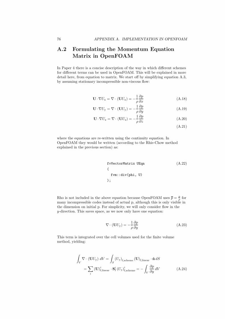
76 APPENDIX A. IMPLEMENTATION IN OPENFOAM
A.2 Formulating the Momentum EquationMatrix in OpenFOAM
In Paper 4 there is a concise description of the way in which different schemesfor different terms can be used in OpenFOAM. This will be explained in moredetail here, from equation to matrix. We start off by simplifying equation A.3,by assuming stationary incompressible non-viscous flow:
U · ∇Ux = ∇ · (UUx) = −1
ρ
∂p
∂x(A.18)
U · ∇Uy = ∇ · (UUy) = −1
ρ
∂p
∂y(A.19)
U · ∇Uz = ∇ · (UUz) = −1
ρ
∂p
∂z(A.20)
(A.21)
where the equations are re-written using the continuity equation. InOpenFOAM they would be written (according to the Rhie-Chow methodexplained in the previous section) as:
fvVectorMatrix UEqn (A.22)
(
fvm::div(phi, U)
);
Rho is not included in the above equation because OpenFOAM uses p = pρ for
many incompressible codes instead of actual p, although this is only visible inthe dimension on initial p. For simplicity, we will only consider flow in they-direction. This saves space, as we now only have one equation:
∇ · (UUy) = −1
ρ
∂p
∂y(A.23)
This term is integrated over the cell volumes used for the finite volumemethod, yielding:
∫
V
∇ · (UUy) dV =
∫
S
(Uy)f,scheme (U)f,linear · n dS
=∑
i
(U)if,linear ·Sif (Uy)
if,scheme = −
∫
V
∂p
∂ydV (A.24)
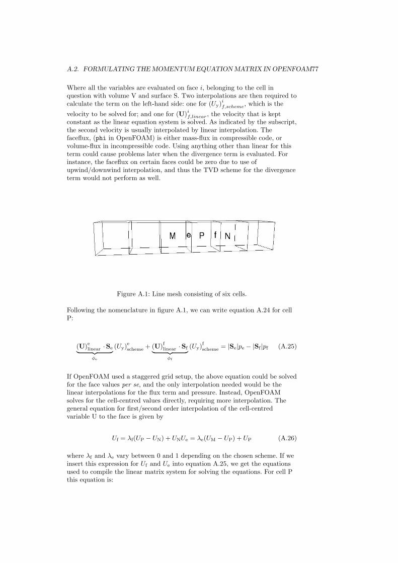
A.2. FORMULATING THE MOMENTUM EQUATION MATRIX IN OPENFOAM77
Where all the variables are evaluated on face i, belonging to the cell inquestion with volume V and surface S. Two interpolations are then required tocalculate the term on the left-hand side: one for (Uy)
if,scheme, which is the
velocity to be solved for; and one for (U)if,linear , the velocity that is kept
constant as the linear equation system is solved. As indicated by the subscript,the second velocity is usually interpolated by linear interpolation. Thefaceflux, (phi in OpenFOAM) is either mass-flux in compressible code, orvolume-flux in incompressible code. Using anything other than linear for thisterm could cause problems later when the divergence term is evaluated. Forinstance, the faceflux on certain faces could be zero due to use ofupwind/downwind interpolation, and thus the TVD scheme for the divergenceterm would not perform as well.
Figure A.1: Line mesh consisting of six cells.
Following the nomenclature in figure A.1, we can write equation A.24 for cellP:
(U)elinear ·Se
︸ ︷︷ ︸
φe
(Uy)escheme + (U)
flinear ·Sf
︸ ︷︷ ︸
φf
(Uy)fscheme = |Se|pe − |Sf |pf (A.25)
If OpenFOAM used a staggered grid setup, the above equation could be solvedfor the face values per se, and the only interpolation needed would be thelinear interpolations for the flux term and pressure. Instead, OpenFOAMsolves for the cell-centred values directly, requiring more interpolation. Thegeneral equation for first/second order interpolation of the cell-centredvariable U to the face is given by
Uf = λf(UP − UN) + UNUe = λe(UM − UP) + UP (A.26)
where λf and λe vary between 0 and 1 depending on the chosen scheme. If weinsert this expression for Uf and Ue into equation A.25, we get the equationsused to compile the linear matrix system for solving the equations. For cell Pthis equation is:
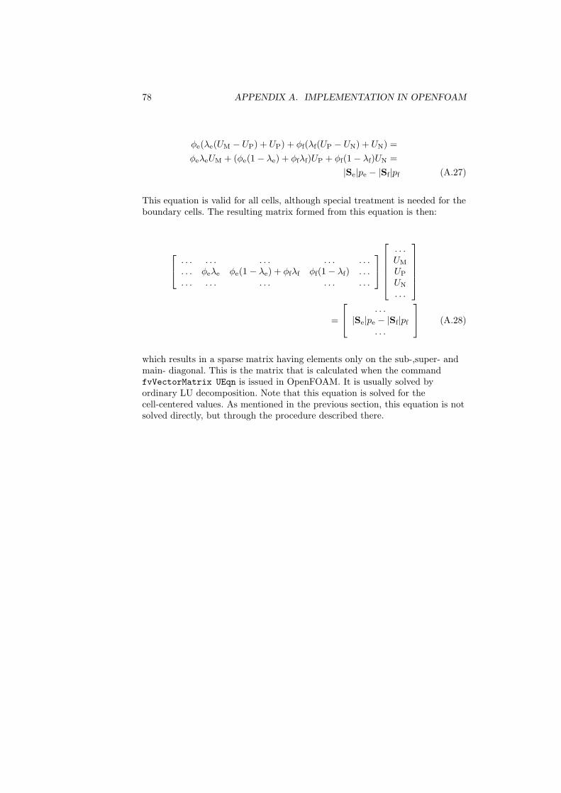
78 APPENDIX A. IMPLEMENTATION IN OPENFOAM
φe(λe(UM − UP) + UP) + φf(λf(UP − UN) + UN) =
φeλeUM + (φe(1 − λe) + φfλf)UP + φf(1 − λf)UN =
|Se|pe − |Sf|pf (A.27)
This equation is valid for all cells, although special treatment is needed for theboundary cells. The resulting matrix formed from this equation is then:
. . . . . . . . . . . . . . .
. . . φeλe φe(1 − λe) + φfλf φf(1 − λf) . . .
. . . . . . . . . . . . . . .
. . .UM
UP
UN
. . .
=
. . .|Se|pe − |Sf|pf
. . .
(A.28)
which results in a sparse matrix having elements only on the sub-,super- andmain- diagonal. This is the matrix that is calculated when the commandfvVectorMatrix UEqn is issued in OpenFOAM. It is usually solved byordinary LU decomposition. Note that this equation is solved for thecell-centered values. As mentioned in the previous section, this equation is notsolved directly, but through the procedure described there.
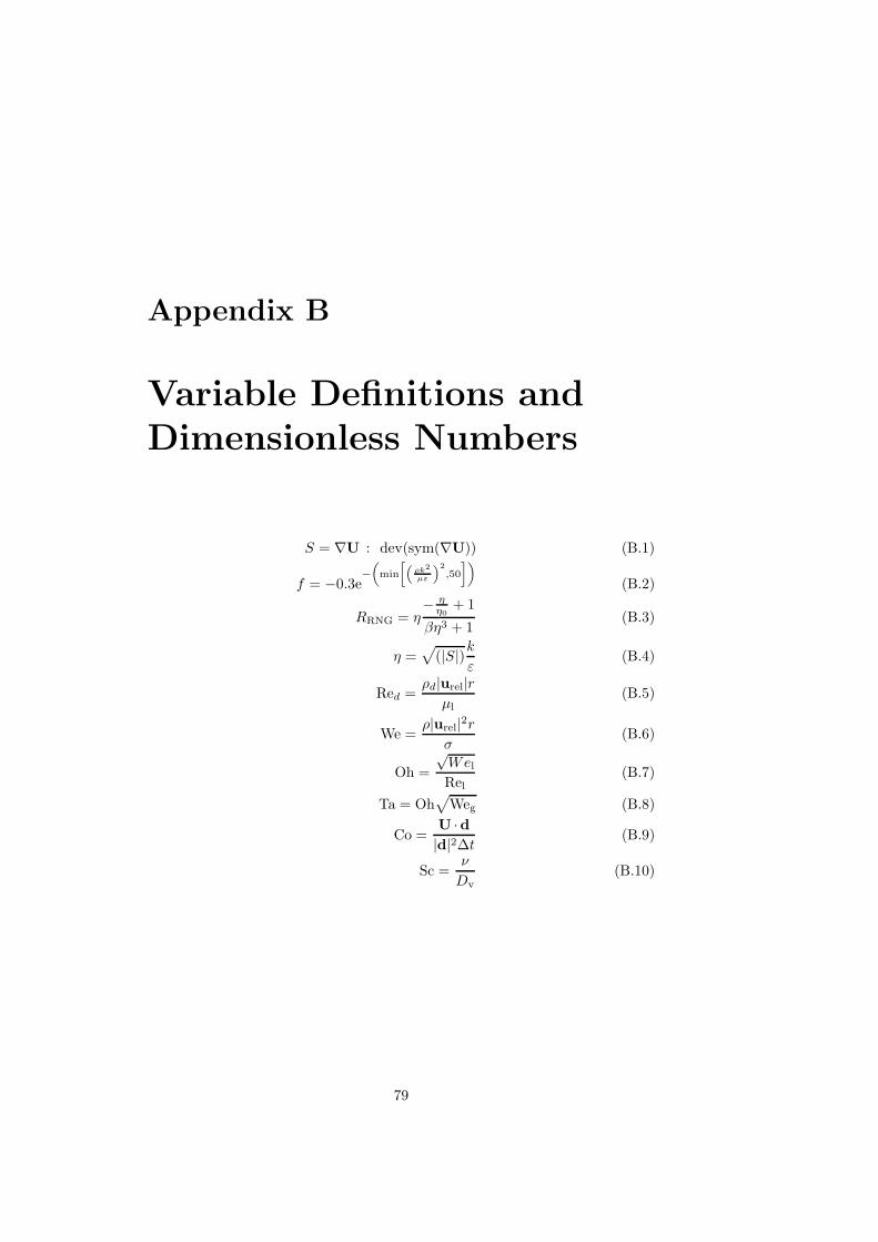
Appendix B
Variable Definitions andDimensionless Numbers
S = ∇U : dev(sym(∇U)) (B.1)
f = −0.3e−
„
min
»
“
ρk2
µε
”2
,50
–«
(B.2)
RRNG = η− ηη0
+ 1
βη3 + 1(B.3)
η =√
(|S|)kε
(B.4)
Red =ρd|urel|r
µl(B.5)
We =ρ|urel|2r
σ(B.6)
Oh =
√WelRel
(B.7)
Ta = Oh√
Weg (B.8)
Co =U ·d|d|2∆t (B.9)
Sc =ν
Dv(B.10)
79
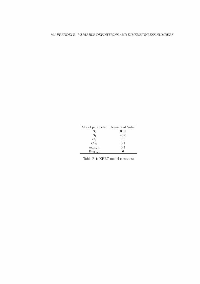
80APPENDIX B. VARIABLE DEFINITIONS AND DIMENSIONLESS NUMBERS
Model parameter Numerical ValueB0 0.61B1 40.0Cτ 1.0CRT 0.1ms,limit 0.4Welimit 6
Table B.1: KHRT model constants
Bibliography
[1] Tarr, J.A. and McShane, C., 1997. “The centrality of the horse to thenineteenth-century american city”. In The Making of Urban America.Scholarly Resources Inc., pp. 105–130.
[2] World Health Organization, 2003. “Health aspects of air pollution withparticulate matter, ozone and nitrogen dioxide”. EUR/03/5042688.
[3] Kageson, Per, www.bilsweden.se. Dieselmotorn pa kort och lang sikt.
[4] www.dieselnet.com/standards/eu/ld.html, 2007. Emission standards.
[5] United States Environmental Protection Agency, 2007. Light-DutyAutomotive Technology and Fuel Economy Trends: 1975 through 2007.
[6] Lagerquist, M., 2007. Energilaget i siffror 2007, Energy in Sweden 2007Facts and Figures.
[7] Patterson, M.A., Kong, S.C, Hampson, G.J. and Reitz, Rolf D., 1994.“Modeling the Effects of Fuel Injection Characteristics on Diesel EngineSoot and NOx Emissions”. SAE Paper 940523.
[8] Patterson, M., and Reitz, R. D., 1998. “Modeling the effects of fuel spraycharacteristics on diesel engine combustion and emission”. SAE Paper980131.
[9] O’Rourke, P.J., and Amsden, A.A., 1987. “The tab method for numericalcalculation of spray droplet breakup”. SAE Paper 872089.
[10] Weller, H., Tabor, G., Jasak, H., and Fureby, C., 1998. “A TensorialApproach to Computational Continuum Mechanics using ObjectOrientated Techniques”. Computers in Physics, 12(6), pp. 620–631.
[11] Jasak, H., Weller, H. G. and Nordin, N., 2004. “In-Cylinder CFDSimulation Using a C++ Object-Oriented Toolkit”. SAE Paper2004-01-0110.
[12] Stiesch, G., 2003. Modeling Engine Spray and Combustion Processes.Springer Verlag Berlin Heidelberg New York.
[13] Faeth, G. M., Hsiang, L-P and Wu, P-K, 1995. “Structure and BreakupProperties of Sprays”. International Journal of Multiphase Flow, 21,pp. 99–127.
81
82 BIBLIOGRAPHY
[14] Badock, C., Wirth, R., Fath, A., and Leipertz, A., 1999. “Investigation ofcavitation in real size diesel injection nozzles”. International Journal ofHeat and Fluid Flow, 20(5).
[15] Winklhofer, E., Kull, E., Kelz, E., and Morozov, A., 2001.“Comprehensive Hydraulic and Flow Field Documentation in ModelThrottle Experiments Under Cavitation Conditions”. In Proceedings ofthe ILASS-Europe Annual Meeting, Zurich, Switzerland, pp. 574–579.
[16] Arcoumanis, C., Gavaises, M., Flora, H., Roth, H., 2001. “Visualisation ofcavitation in diesel engine injectors”. Mecanique & Industries, 2(5).
[17] Blessing, M., Konig, G., Kruger, C., Michels, U., and Schwarz, V., 2003.“Analysis of Flow and Cavitation Phenomena in Diesel Injection Nozzlesand its Effects on Spray and Mixture Formation”. SAE Paper2003-01-1358.
[18] Schmidt, D., Rutland, C., and Corradini, M., 1997. “A numerical study ofcavitating flow through various nozzle shapes”. SAE Paper 971597.
[19] Yuan, W., and Schnerr, G., 2003. “Numerical Simulation of Two-PhaseFlow in Injection Nozzles: Interaction of Cavitation and External JetFormation”. Journal of Fluids Engineering, 125, pp. 963–969.
[20] Mulemane, A., Subramaniyam, S., Lu, P., Han, J., Lai, M., and Poola, R.,2004. “Comparing Cavitation in Diesel Injectors Based on DifferentModeling Approaches”. SAE Paper 2004-01-0027.
[21] Martynov, S., Mason, D., Heikal, M. R., Sazhin, S. S., and Gorokhovski,M., 2006. “Modelling of Cavitation Flow in a Nozzle and its Effect onSpray Development”. In International Heat Transfer Conference.
[22] Yuan, W., Sauer, J., and G.H., S., 2001. “Modeling and Computation ofUnsteady Cavitation Flows in Injection Nozzles”. Mechanique &Industries, 2, pp. 383–394.
[23] Masuda, R., Fuyuto, T., Nagaoka, M., Berg, E., and Tatschl, R., 2005.“Validation of diesel fuel spray and mixture formation from nozzleinternal flow calculation”. SAE Paper 2005-01-2098.
[24] Ning, W., 2007. “Development of a next-generation spray andatomization model using an eulerian-lagrangian methodology”. PhDthesis, University of Wisconsin - Madison.
[25] Roth, H., Giannadakis, E., Gavaises, M., Arcoumanis, C., Omae, K.,Sakata, I., Nakamura, M., and Yanagihara, H., 2005. “Effect ofmulti-injection strategy on cavitation development in diesel injectornozzle holes”. SAE Paper 2005-01-1237.
[26] Nouri, J., Mitroglou, N., Yan, Y., and Arcoumanis, C., 2007. “Internalflow and cavitation in a multi-hole injector for gasoline direct-injectionengines”. SAE Paper 2007-01-1405.
BIBLIOGRAPHY 83
[27] Payri, R., Margot, X., and Salvador, F., 2002. “A Numerical Study of theInfluence of Diesel Nozzle Geometry on the Inner Cavitating Flow”. SAEPaper 2002-01-0215.
[28] Schmidt, D.P., Rutland, C.J. and Corradini, M.L., 1999. “A FullyCompressible Two-Dimensional Model of High Speed CavitatingNozzles”. Atomization and Sprays, 9.
[29] Vortmann, C., Schnerr, G., and Seelecke, S., 2003. “ThermodynamicModeling and Simulation of Cavitating Nozzle Flow”. InternationalJournal of Heat and Fluid Flow, 24.
[30] Weller, H. G., 2006. A New Approach to VOF-based Interface CapturingMethods for Incompressible, Compressible and Cavitating Flow. Tech.Rep. TR/HGW/07, OpenCFD Ltd., October.
[31] Wallis, G. B., 1969. One-dimensional Two-phase Flow. McGraw-Hill,New York.
[32] Chung, M.-S., Park, S.-B., and Lee, H.-K., 2004. “Sound speed criterionfor two-phase critical flow”. Journal of Sound and Vibration, 276,pp. 13–26.
[33] Ubbink, O., 1997. “Numerical prediction of two fluid systems with sharpinterfaces”. PhD thesis, Imperial College.
[34] Poinsot, T.J., and Lele, S.K., 1992. “Boundary conditions for directsimulations of compressible viscous reacting flows”. Journal ofComputational Physics, 101, pp. 103–129.
[35] Huh, K.Y., and Gosman, A.D., 1990. “Atomization Mechanism of FuelInjection”. ILASS.
[36] Kralj, C., 1995. “Numerical Simulation of Diesel Spray Processes”. PhDthesis, Imperial College of Science Technology and Medicine.
[37] Peng, D.-Y., and Robinson, D. B., 1976. “A new two-constant equation ofstate”. Industrial & Engineering Chemistry Fundamentals, 15, pp. 59–64.
[38] Xie, W. F., Liu, T. G., and Khoo, B. C., 2006. “Application of a one-fluidmodel for large scale homogeneous unsteady cavitation: The modifiedSchmidt model”. Computers & Fluids, 35, pp. 1177–1192.
[39] de Villiers, E., Gosman, A., and Weller, H., 2004. “Large Eddy Simulationof Primary Diesel Spray Atomization”. SAE Paper 2004-01-0100.
[40] Befrui, B., Corbinelli, G., Robart, D., and Reckers, W., 2008. “LESSimulation of the Internal Flow and Near-Field Spray Structure of anOutward-Opening GDi Injector and Comparison with Imaging Data”.SAE Paper 2008-01-0137.
[41] Menard, T., and Berlemont, A., 2007. “Interface tracking with a coupledlevel set/vof/ghost fluid method: Application to jet atomization”.Proceedings of FEDSM2007, FEDSM2007-37377.
84 BIBLIOGRAPHY
[42] Vuorinen, V., Larmi, M., and Fuchs, L., 2008. “Large-Eddy Simulation onthe Effect of Droplet Size Distribution on Mixing of Passive Scalar in aSpray”. SAE Paper 2008-01-0933.
[43] Blokkeel, G., Barbeau, B., and Borghi, R., 2003. “A 3D Eulerian Modelto Improve the Primary Breakup of Atomizing Jet”. SAE Paper2003-01-0005.
[44] Lebas, R., Blokkeel, G., Beau, P.-A., and Demoulin, F.-X., 2005.“Coupling Vaporization Model With the Eulerian-Lagrangian SprayAtomization (ELSA) Model in Diesel Engine Conditions”. SAE2005-01-0213.
[45] Iyer, V. and Abraham, J., 2003. “An Evaluation of a Two-FluidEulerian-Liquid Eulerian-Gas Model for Diesel Sprays”. Journal of FluidsEngineering, 125, pp. 660–669.
[46] Jones, W. and Launder, B., 1972. “The prediction of laminarization witha two-equation model of turbulence”. Int. J. Heat Mass Transfer, 15,pp. 301–314.
[47] Yakhot, V. and Orzag, S.A., 1986. “Renormalization Group Analysis ofTurbulence”. I. Basic Theory J. Sci. Comput.
[48] Launder, B. and Sharma, B., 1975. “Application of the energy dissipationmodel of turbulence to the calculation of flow near a spinning disc”. Lett.Heat and Mass Transfer, 1, pp. 131–138.
[49] Amsden, A.A., O’Rourke, P.J. and Butler, T.D., 1989. “Kiva-ii: Acomputer program for chemically reactive flows with sprays”.LA-11560-MS, May.
[50] Gore, R., and Crowe, C. T., 1989. “Effect of particle size on modulatingturbulent intensity”. International Journal of Multiphase Flow, 15(2),pp. 279–285.
[51] Crowe, C., Sommerfeld, M., and Tsuji, Y., 1998. Multiphase Flows withDroplets and Particles. CRC Press LLC.
[52] Nordin, N., 2001. “Complex chemistry modeling of diesel spraycombustion”. PhD thesis, Dept. of Thermo and Fluid Dynamics,Chalmers University of Technology, Goteborg.
[53] Press, W.H., Teukolsky, S.A., Vetterling, W.T. and Flannery, B.P., 2002.Numerical Recipes in C++: The Art of Scientific Computing, 2:nd ed.Cambridge University Press.
[54] Karlsson, J. A. J., 1995. “Modeling Auto-Ignition, Flame Propagationand Combustion in Non-stationary Turbulent Sprays”. PhD thesis,Chalmers University of Technology, Goteborg.
[55] Venugopal, R., and Abraham, J., 2007. “A numerical investigation offlame lift-off in diesel jets”. Combustion Science and Technology, 179,pp. 2599–2618.
BIBLIOGRAPHY 85
[56] P.K. Senecal, E. P., and Richards, K., 2003. “Multidimensional Modelingof Direct-Injection Diesel Spray Liquid Length and Flame Lift-off Lengthusing CFD and Parallel Detailed Chemistry”. SAE 2003-01-1043.
[57] Tap, F., and Veynante, D., 2005. “Simulation of Flame Lift-off on aDiesel Jet Using a Generalized Flame Surface Density Approach”.Proceedings of Combustion Inst.(30), pp. 919–926.
[58] Chomiak, J. and Karlsson, J.A.J., 1996. “Flame Liftoff in Diesel Sprays”.Twenty-Sixth Symposium (International) on Combustion/TheCombustion Institute, pp. 2557–2564.
[59] Tao, F., 2003. “Numerical Modeling of Soot and NOx Formation inNon-Stationary Diesel Flames with Complex Chemistry”. PhD thesis,Chalmers University of Technology, Goteborg.
[60] Macpherson, G. B., Nordin, N., and Weller, H. G., 2008. “Particletracking in unstructured, arbitrary polyhedral meshes for use in cfd andmolecular dynamics”. Communications in Numerical Methods inEngineering.
[61] Schmalzing, C.-O, Stapf, P., Maly, R.R., Renner, G., Stetter, H., andDwyer, H.A., 1999. “A holistic hydraulic and spray model - liquid andvapor phase penetration of fuel sprays in di diesel engines”. SAE Paper1999-01-3549.
[62] Kimura, S., Kosaka, H., Matsui, Y.,and Himeno, R., 2004. “A numericalsimulation of turbulent mixing in transient spray by les”. SAE Paper2004-01-2014.
[63] Reitz, R.D., 1987. “Modeling Atomization Processes in High-PressureVaporizing Sprays”. Atomization and Spray Technology, 3, pp. 309–337.
[64] Park, S. W., Kim, H. J., and Lee, C. S., 2003. “Investigation ofatomization characteristics and prediction accuracy of hybrid models forhigh-speed diesel fuel sprays”. SAE Paper 2003-01-1045.
[65] Rotondi, R., Bella, G., Grimaldi, C., and Postrioti, L., 2001.“Atomization of High-Pressure Diesel Spray: Experimental Validation of aNew Breakup Model”. SAE paper 2001-01-1070.
[66] Bianchi, G.M., and Pelloni, P., 1999. “Modeling the diesel fuel spraybreakup by using a hybrid model”. SAE Paper 1999-01-0226.
[67] Lee, J-H and Goto, S., 2000. “Comparison of spray characteristics inbutane and diesel fuels by numerical analysis”. SAE Paper 2000-01-2941.
[68] O’Rourke, P., 1981. “Collective Drop Effects on Vaporizing LiquidSprays”. PhD thesis, Department of Mechanical and AerospaceEngineering, Princeton University.
[69] Schmidt, D., and Rutland, C., 2000. “A New Droplet CollisionAlgorithm”. Journal of Computational Physics, 164, pp. 62–80.
86 BIBLIOGRAPHY
[70] Gustavsson, J., and Golovitchev, V., 2004. “3D Simulation of MultipleInjections in DI Diesel Engine”. In The Sixth International Symposiumon Diagnostics and Modeling of Combustion in Internal CombustionEngines, COMODIA.
[71] Peng Karrholm, F., 2006. Numerical Modelling of Diesel Spray Injectionand Turbulence Interaction. Licentiate Thesis, Department of AppliedMechanics, Chalmers University of Technology.
[72] van Leer, B., 1977. “Towards the ultimate conservative difference schemeiii. upstream-centered finite-difference schemes for ideal compressibleflow”. J. Comp. Phys., 23, pp. 263–75.
[73] Sandia National Laboratories, 2007. Engine combustion network(public.ca.sandia.gov/ecn).
[74] Hilbert, R., and Thevenin, D., 2002. “Autoignition of turbulentnonpremixed flames investigated using direct numerical simulations”.Combustion and Flame, 128, pp. 22–37.
[75] Hilbert, R., Tap, F., El-Rabii, H., and Thevenin, D., 2004. “Impact ofdetailed chemistry and transport models on turbulent combustionsimulations”. Progress in Energy and Combustion Science, 30,pp. 61–117.
[76] Siebers, D. L., and Higgins, B. S., 2000. Effects of Injector Conditions onthe Flame Lift-Off Length of DI Diesel Sprays. Tech. Rep. 2000-8249,Sandia National Laboratories.
[77] Husberg, T., Denbratt, I., and Karlsson, A., 2008. “Analysis of advancedmultiple injection strategies in a heavy-duty diesel engine using opticalmeasurements and cfd simulations”. SAE Paper 2008-01-1328.
[78] Payri, F., Bermudez, V., Payri, R., and Salvador, F., 2004. “The influenceof cavitation on the internal flow and the spray characteristics in dieselinjection nozzles”. Fuel, 83, pp. 419–431.
[79] Gavaises, M., Arcoumanis, C., Roth, H., Choi, Y., and Theodorakakos,A., 2002. “Nozzle flow and spray characteristics from vco diesel injectornozzles”. SAE Paper 2002-30-0002.
[80] Lucchini, T., D’Errico, G., Jasak, H., and Tukovic, Z., 2007. “Automaticmesh motion with topological changes for engine simulation”. SAE Paper2007-01-0170.
[81] Ochoterena, R., Larsson, M., Andersson, S., and Denbratt, I., 2008.“Optical studies of spray development and combustion characterization ofoxygenated and fischer-tropsch fuels”. SAE Paper 2008-01-1393.
[82] Ferziger, J.H. and Peric, M., 1999. Computational Methods for FluidDynamics. Springer.

Paper II

MODELLING INJECTOR FLOW INCLUDING CAVITATION EFFECTS FOR D IESELAPPLICATIONS
F. Peng K arrholm ∗
Department of Applied MechanicsChalmers University of Technology
SwedenEmail: [email protected]
Henry WellerOpenCFD Ltd.
Caversham, ReadingUK
Niklas NordinScania CV AB
SodertaljeSweden
Proceedings of FEDSM2007 5th Joint ASME/JSME Fluids Engineering Conference
July 30-August 2, 2007 San Diego, California USA
FEDSM2007-37518
ABSTRACTIn this paper, cavitation and pressure parameters measur
in a model diesel injector are compared to data acquired by n-merical simulations using a new code developed for the OpeFOAM platform, which uses a barotropic equation of state together with the homogeneous equilibrium assumption. It isviscid code, allowing both compressible liquid and vapour tobe modelled. The mass flow and cavitation probabilities otained from the simulations are compared to data obtainedexperiments performed at AVL’s laboratories, in which the flowthrough an almost two-dimensional nozzle was examined. Texperimental data used include pressure profiles and cavitationimages. The model proved to be able to predict cavitation prob-abilities, mass flows, and the occurrence of super-cavitation inthe channel. In addition, it proved to be stable in its dependencyon physical parameters, and grid independent.
NOMENCLATUREA flow area of the nozzleAi area of a face in the nozzle in flow directionCd discharge coefficientp pressure∆ p pressure differenceU velocitym mass flowγ vapour fraction
∗Address all correspondence to this author.
1
edun--a
b-in
he
µg vapour viscosityµl liquid viscosityµf fluid viscosityρ fluid densityρv vapour densityρl liquid densityρv,sat vapour density at saturationρl ,sat liquid density at saturationψv vapour compressibilityψl liquid compressibility
INTRODUCTIONIn Diesel engines and direct injection spark ignition engines,
fuel is injected into the combustion chamber by high pressure.Ideally, the fuel should atomise, form small droplets, and even-tually evaporate completely in order to obtain a mixture that canbe easily combusted without formation of soot orNOx. Impor-tant features of the atomisation, including the size of the initialdroplets and the fragmentation processes, are mainly governedby the flow in the nozzle [1] which ejects the spray. It is there-fore important to study the flow inside the nozzle, to find out howit is linked to the flow in the combustion cylinder.
When a high velocity fluid passes through a contraction likea nozzle, a pocket of low pressure is formed in the wake of itsedge. In this wake the pressure can decrease below the satura-tion pressure, and thus cause the liquid to cavitate. The size ofthe cavitation bubbles thereby formed depends on several fac-tors, including (inter alia) the injection pressure, geometry, and
Copyright c© 2007 by ASMECopyright © 2007 Chalmers University of Technology
smoothness of the interior of the nozzle, and the propertiesof thefluid. For example, if the fluid is pushed through the nozzle suf-ficiently slow, there will be no cavitation and ordinary pipeflowwill occur.
Cavitation introduces vapour bubbles into the flow. It alsincreases the maximum velocity, for two reasons. If therevapour along the walls, the liquid will not have a no-slip bound-ary condition, since the vapour by the wall will not be station-ary. This allows a higher velocity of the liquid, which is requiredwhen the pressure over the nozzle is high. The velocity is aoincreased since the liquid can not fill the entire channel. Whenthe vapour bubbles formed in the nozzle reach the combustchamber, both the bubbles and the liquid surrounding them wllbe heated by the gas in the chamber. The liquid will evaporafaster if it has already been partially evaporated by cavitation,and thus the entire atomisation process will be accelerated.
The point where the fluid is no longer cavitating is callethe re-attachment point, if there is no such point the fluid will besuper-cavitating and the cavitation region will extend through-out the entire nozzle. Super-cavitation changes the atomisationbehaviour significantly, since the spray’s cone angle is severelyreduced when it exits the injector, resulting in a steady flowwithfairly large scale disturbances on the surface [2]. Therefore,super-cavitation should be avoided, since it severely reduces theatomisation. There are also other negative aspects of cavitationaside from super-cavitation. Notably it can erode the injector,thus reducing its lifetime. Further, if the injection pressure is in-creased, for a cavitating injector the flow rate is still constant.This removes the option of increasing spray penetration by usinghigher pressures, and thus higher atomisation. Ultimatelyit willimpair performance of the engine.
PREVIOUS STUDIES ON CAVITATION IN NOZZLESNumerical studies on Diesel sprays are usually based
Euler-Lagrangian modelling according to the Discrete DropletModel (DDM). Few attempts have been made to model the etire spray using only an Eulerian framework, and those that havebeen made have usually been done in 2D [3] or have been liited to a restricted part of the spray [4]. There are also hybrids,like the model described in [5], in which Lagrangian parcelsareadded to the spray when the liquid phase is sufficiently disperse.However, the most common way of modelling sprays is still tuse a combination of Eulerian gas and Lagrangian liquid descrip-tions. Associated with the DDM model are several sub-modedescribing injection, atomisation, break-up, evaporation, com-bustion etc.
The injection model will be described further, as it is oparticular interest when studying cavitation. One of the mostcommon approaches when modelling injection is to assumedroplets follow a distribution with some estimated parameters,and then sample the droplet size from that distribution. This type
2
ois
ls
ionite
d
on
n-
m-
o
ls
f
the
of model was used in [6–8]. More ambitious injection models,which attempt to couple the nozzle flow to the injected droplets,have been presented [9–11]. However, their rationale has notbeen based on CFD or experimental data, but on theoretical con-siderations and assumptions. This paper focuses on verifying acode for a cavitating injector, thereby providing a sound founda-tion for the subsequent development of a new injection model.
Previous works related to cavitation in nozzles under dieselconditions have focused on various aspects of the associated phe-nomena. One option, adopted by Sarreet al [12], is to use CFDto investigate the nozzle flow and couple it to the spray. Sarreet al focused on the spray calculations, and the effect the flow inthe nozzle has on the spray, rather than studying the actual nozzleflow. In other studies only the nozzle flow has been simulated,e.g. the study by Mulemaneet al [13], in which two of the possi-ble modelling approaches to cavitation was explored. The citedauthors present pressure plots similar to those in this article, butdo not compare their numerical results with experimental data.
There is also a study by Yuanet al [2], in which the cavi-tating flow inside the nozzle as well as the atomising spray closeto the nozzle is modelled. This approach is not common, dueto the complexities associated with the presence of three phases:liquid, vapour formed from the cavitated liquid, and gas whichthe liquid is being injected into. Diesel injection into airwithoutcavitation has also been simulated in [4].
Cavitation can be modelled in several ways. There are inter-face tracking methods, which have two explicit phases, and con-tinuum methods which have just one explicit phase. Continuummethods include the Rayleigh-Plesset bubble method [14, 15],barotropic equation of state method [13, 16], and a third rarelyused method based on Gibbs free energy [17].
The method chosen for cavitation modelling for this workis the barotropic equation of state approach, mainly because it ismost appropriate for the cavitation that occurs in diesel injectors,which originates from flow separation at the nozzle inlet. TheRayleigh-Plesset (RP) approach is therefore unsuitable, since itis based on the specified bubble density, and assumes gas diffu-sion and bubble coalescence to be important factors [13]. How-ever, since the velocity in diesel injectors is high, diffusion andbubble coalescence can be assumed to have negligible effects.Further, the code we used is a simplified Volume of Fluid (VOF)code that allows both diesel vapour and air to be modelled. Sincethe Barotropic equation of state is more consistent with theVOFframework, it was deemed to the most suitable method for thiswork.
The barotropic equation of state method described in [13]differs from the one used here in the sense that it assumed thetwofluid phases to be incompressible. In this paper both phases arecompressible, which increases the physical validity. It also dif-fers from the one presented by Schmidt [16], in which an equa-tion of state is analytically integrated, and thus the pressure isfound as a function of density.
Copyright c© 2007 by ASMECopyright © 2007 Chalmers University of Technology
Experimental data in the field are very scarce, and manmodels have only been validated (if at all) by comparing simulated and empirical discharge coefficients, cavitation numbersand average velocities. This is due to the difficulties involved inexperimentally investigating the nozzle flow. Often the cavita-tion along the sides of the nozzle makes it very difficult to eval-uate the flow inside, since the cavitation hinders optical analysis.However, in experiments presented in [18] a nozzle was set upinsuch a way that cavitation was limited to two of the four sidesofthe nozzle, thus allowing the pressure and velocities of theflowto be measured. The data acquired in these experiments are uedto validate the model presented in this article.
The main objective of this paper is to introduce the newmodel, by first describing the theory underlying the equation ofstate (EOS) used, and then the momentum equations and hthey are solved. The experimental case study used to comparetothe simulations is briefly described, and the numerical setup. Fi-nally, results are presented, including both pressure profile com-parisons and cavitation probability images.
THEORYTo model the flow in the nozzle, we need to model the cav
itation, and either resolve the turbulent scales or model them.Turbulence is not modelled, due to the relatively weak influenceit is believed to have on the nozzle flow, compared to the cavita-tion [14]. The only way turbulence is addressed is in stabilisingnumerics (in contrast to DNS computations) which are not suffi-ciently accurate to include all scales of the turbulence. Asmen-tioned above, the barotropic equation of state was the methdchosen for modelling cavitation. We also assumed homogenosequilibrium, i.e. the liquid and vapour are assumed to alwaysbe perfectly mixed in each cell. The parameterγ describes theamount of cavitated vapour in each cell.
For the method chosen to model the cavitation, an equatioof state is needed. The temperature is assumed to be consta,which is not a major limitation [18]. A common barotropic equa-tion of state is the non-equilibrium differential equation:
DρDt
= ψDpDt
(1)
ψ refers to the compressibility, which is the inverse squarroot of the speed of sound in the cavitating mixture. This equa-tion can either be used directly in the continuity equation to for-mulate a pressure equation, or integrated to obtain the pressureas a function of the density. The latter approach was adoptedbySchmidtet al [16], as mentioned earlier. The former approachis problematic because equation 1 is not an equilibrium equationof state, so the pressure and density obtained are not consistentwith the liquid and vapour equations of state unless equilibrium
3
y-
s
ow
-
ou
nnt
e
has been reached. Before equilibrium is attained errors will arise,and the code will not yield corrects result when it has been at-tained.
The equation of state should therefore be consistent with theliquid and vapour equations of state both at the limits when thereis pure liquid or pure vapour, and at intermediate states whenthere is some form of mixture. The two states can be describedby the linear equation of state:
ρv = ψvp (2)
ρl = ρ0l + ψl p (3)
The parameter that describes how much of the liquid is ineach phase isγ:
γ =ρ−ρl ,sat
ρv,sat−ρl ,sat(4)
γ = 1 corresponds to a fully cavitated flow, andγ = 0 a flowwith no cavitation.ρv,sat is calculated from
ρv,sat = ψvpsat (5)
ψv is the compressibility of the vapour. These propertiestogether form the mixture’s equilibrium equation of state:
ρ = (1− γ)ρ0l +(γψv +(1− γ)ψl ) psat
+ψ(γ)(
p− psat) (6)
The compressibilityψ was first mentioned in equation 1, butnothing was said of how it is chosen. It can be modelled in sev-eral ways, one very common way is the Wallis model [19]. Themodel chosen here is a simple linear one:
ψ = γψv +(1− γ)ψl (7)
A linear model was selected partly because the code we usedis based on a VOF code, for which linear combinations ofγ arehighly suitable for describing the mixtures properties, and partlybecause it gives greater stability than the Wallis model. The γvalue is also used to calculate the mixture’s viscosity, in the samemanner as the compressibility:
Copyright c© 2007 by ASMECopyright © 2007 Chalmers University of Technology
µf = γµv +(1− γ)µl (8)
When a linear model is used for the compressibility, theequation of state (6) can be simplified into:
ρ = (1− γ)ρ0l + ψp (9)
The first term governs the liquid’s density whenγ is low. Ifthe fluid is cavitated, the second term becomes more dominan.The first term contains the propertyρ0
l which is:
ρ0l = ρl ,sat− psatψl (10)
ρl ,sat is the liquid density at standard conditions. The sat-uration density of the vapour, previously used to calculateγ, isimportant for the liquid’s tendency to cavitate. A higherρv,sat
will not require as lowρ to get a higherγ.Unlike the model used by Schmidtet al [16], the code does
not solve the Euler equations for inviscid flow to obtain the veloc-ity and density. Viscous terms are included, and the momentumequations are solved for U, notρ U which is common for friction-free compressible flows. A brief description of the methodologyof the code is given for clarity. The iteration process starts bysolving the continuity equation (eq. 11) forρ, which is whererho is convected.
∂ρ∂t
+ ∇ · (ρU) = 0 (11)
Theρ in the divergence term∇ · (ρU) is interpolated by useof a total variation diminishing (TVD) scheme named MUSCL.The MUSCL scheme is second order in space, and appropriawhen there are large gradients present, like the one betweenliq-uid and vapor density. Several other options are easily availablein the code.ρ is also used to obtain preliminary values forγ (eq.4) andψ (eq. 7), and when defining the momentum equations.
∂ρU∂t
+ ∇ · (ρUU) = −∇p+ ∇(µf ∇U) (12)
The momentum equations are used in an ordinary fashion tget the matrices used to calculate the pressure-free velocity. The
4
t
te
o
same TVD scheme with MUSCL limiter is used for the velocitydivergence term. It was found to be very important to choose aproper scheme for the velocity, if a too stable scheme is usedthecavitation region will be flat. Following this is an ordinaryPISOloop, to solve for p and correct the velocity to achieve continuity.For a description on how OpenFOAM achieves continuity andsolves for p, see [20]. The equation solved in the PISO loop isagain the continuity equation, but this time transformed into apressure equation by use of equation 6.
∂ψp∂t
−(
ρ0l +(ψl −ψv) psat
) ∂γ∂t
−psat∂ψ∂t
+ ∇ · (ρU) = 0 (13)
When continuity has been reached, the remaining propertiesγ, ρ andψ are updated.ρ is now updated according to the EOS,eq. 6. The time step is limited by both the Courant number, andthe acoustic Courant number, respectively defined as:
Co= max(|U |∆x
)∆t (14)
and
Coacoustic= max(1√ψ∆x
)∆t (15)
The Courant number was chosen to be limited to 0.125, andthe acoustic Courant number was limited to 12.5 in all of thesimulations. However, the non-acoustic Courant number is thereal limiter of the time-step, and the acoustic Courant number isusually around 2-3.
The model described is implemented for the OpenFOAMplatform, under the name cavitatingFoam (in OpenFOAM 1.4).OpenFOAM is an open source toolbox for CFD, written in C++,available at www.openfoam.com.
STUDYThe results produced by the code are compared to data ac-
quired in experiments performed at AVL’s laboratories, in whichdiesel fuel was pumped through a nozzle-like structure. Thesetup is described in [18], and the model nozzle is shown in fig-ure 1. The experiments generated data on density/pressure aswell as images of the cavitation region, and due to the simplicityof the geometry they are suitable for comparison to numerical
Copyright c© 2007 by ASMECopyright © 2007 Chalmers University of Technology
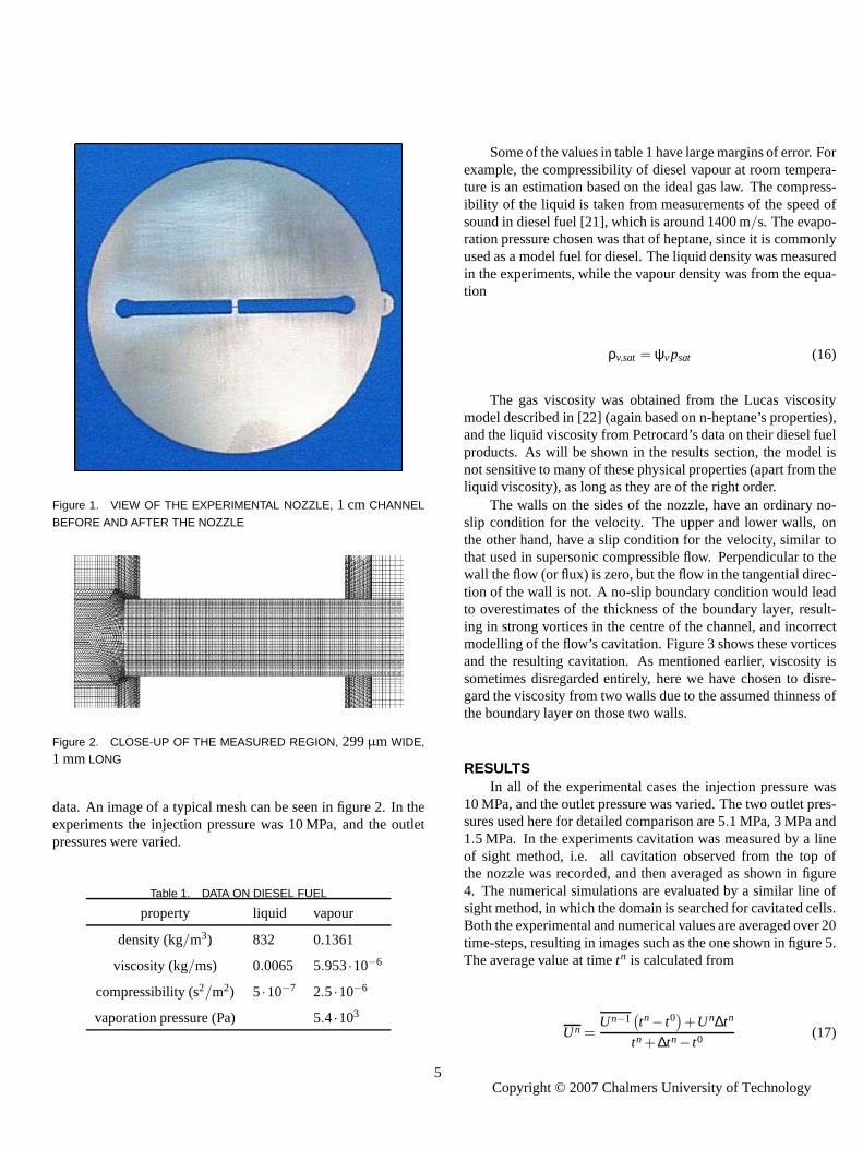
Figure 1. VIEW OF THE EXPERIMENTAL NOZZLE, 1 cmCHANNEL
BEFORE AND AFTER THE NOZZLE
Figure 2. CLOSE-UP OF THE MEASURED REGION, 299µm WIDE,
1 mmLONG
data. An image of a typical mesh can be seen in figure 2. In theexperiments the injection pressure was 10 MPa, and the outletpressures were varied.
Table 1. DATA ON DIESEL FUEL
property liquid vapour
density (kg/m3) 832 0.1361
viscosity (kg/ms) 0.0065 5.953·10−6
compressibility (s2/m2) 5·10−7 2.5·10−6
vaporation pressure (Pa) 5.4·103
5
Some of the values in table 1 have large margins of error. Forexample, the compressibility of diesel vapour at room tempera-ture is an estimation based on the ideal gas law. The compress-ibility of the liquid is taken from measurements of the speedofsound in diesel fuel [21], which is around 1400 m/s. The evapo-ration pressure chosen was that of heptane, since it is commonlyused as a model fuel for diesel. The liquid density was measuredin the experiments, while the vapour density was from the equa-tion
ρv,sat = ψvpsat (16)
The gas viscosity was obtained from the Lucas viscositymodel described in [22] (again based on n-heptane’s properties),and the liquid viscosity from Petrocard’s data on their diesel fuelproducts. As will be shown in the results section, the model isnot sensitive to many of these physical properties (apart from theliquid viscosity), as long as they are of the right order.
The walls on the sides of the nozzle, have an ordinary no-slip condition for the velocity. The upper and lower walls, onthe other hand, have a slip condition for the velocity, similar tothat used in supersonic compressible flow. Perpendicular tothewall the flow (or flux) is zero, but the flow in the tangential direc-tion of the wall is not. A no-slip boundary condition would leadto overestimates of the thickness of the boundary layer, result-ing in strong vortices in the centre of the channel, and incorrectmodelling of the flow’s cavitation. Figure 3 shows these vorticesand the resulting cavitation. As mentioned earlier, viscosity issometimes disregarded entirely, here we have chosen to disre-gard the viscosity from two walls due to the assumed thinnessofthe boundary layer on those two walls.
RESULTSIn all of the experimental cases the injection pressure was
10 MPa, and the outlet pressure was varied. The two outlet pres-sures used here for detailed comparison are 5.1 MPa, 3 MPa and1.5 MPa. In the experiments cavitation was measured by a lineof sight method, i.e. all cavitation observed from the top ofthe nozzle was recorded, and then averaged as shown in figure4. The numerical simulations are evaluated by a similar lineofsight method, in which the domain is searched for cavitated cells.Both the experimental and numerical values are averaged over 20time-steps, resulting in images such as the one shown in figure 5.The average value at timetn is calculated from
Un =Un−1
(
tn− t0)
+Un∆tn
tn + ∆tn− t0 (17)
Copyright c© 2007 by ASMECopyright © 2007 Chalmers University of Technology
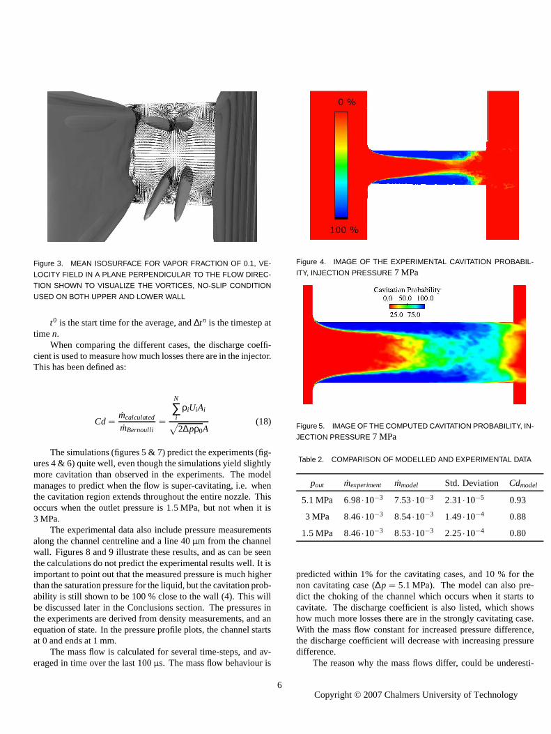
Figure 3. MEAN ISOSURFACE FOR VAPOR FRACTION OF 0.1, VE-
LOCITY FIELD IN A PLANE PERPENDICULAR TO THE FLOW DIREC-
TION SHOWN TO VISUALIZE THE VORTICES, NO-SLIP CONDITION
USED ON BOTH UPPER AND LOWER WALL
t0 is the start time for the average, and∆tn is the timestep attimen.
When comparing the different cases, the discharge coecient is used to measure how much losses there are in the injetor.This has been defined as:
Cd =mcalculated
mBernoulli=
N
∑i
ρiUiAi
√
2∆pρ0A(18)
The simulations (figures 5 & 7) predict the experiments (figures 4 & 6) quite well, even though the simulations yield slightlymore cavitation than observed in the experiments. The momanages to predict when the flow is super-cavitating, i.e. whenthe cavitation region extends throughout the entire nozzle. Thisoccurs when the outlet pressure is 1.5 MPa, but not when it is3 MPa.
The experimental data also include pressure measuremalong the channel centreline and a line 40µm from the channelwall. Figures 8 and 9 illustrate these results, and as can be seenthe calculations do not predict the experimental results well. It isimportant to point out that the measured pressure is much higherthan the saturation pressure for the liquid, but the cavitation prob-ability is still shown to be 100 % close to the wall (4). This willbe discussed later in the Conclusions section. The pressures inthe experiments are derived from density measurements, ananequation of state. In the pressure profile plots, the channelstartsat 0 and ends at 1 mm.
The mass flow is calculated for several time-steps, anderaged in time over the last 100µs. The mass flow behaviour is
6
ffi-c
-
del
ents
d
av-
Figure 4. IMAGE OF THE EXPERIMENTAL CAVITATION PROBABIL-
ITY, INJECTION PRESSURE 7 MPa
Figure 5. IMAGE OF THE COMPUTED CAVITATION PROBABILITY, IN-
JECTION PRESSURE 7 MPa
Table 2. COMPARISON OF MODELLED AND EXPERIMENTAL DATA
pout mexperiment mmodel Std. Deviation Cdmodel
5.1 MPa 6.98·10−3 7.53·10−3 2.31·10−5 0.93
3 MPa 8.46·10−3 8.54·10−3 1.49·10−4 0.88
1.5 MPa 8.46·10−3 8.53·10−3 2.25·10−4 0.80
predicted within 1% for the cavitating cases, and 10 % for thenon cavitating case (∆p = 5.1 MPa). The model can also pre-dict the choking of the channel which occurs when it starts tocavitate. The discharge coefficient is also listed, which showshow much more losses there are in the strongly cavitating case.With the mass flow constant for increased pressure difference,the discharge coefficient will decrease with increasing pressuredifference.
The reason why the mass flows differ, could be underesti-
Copyright c© 2007 by ASMECopyright © 2007 Chalmers University of Technology
Figure 6. IMAGE OF THE EXPERIMENTAL CAVITATION PROBABIL-
ITY, INJECTION PRESSURE 8.5 MPa
Figure 7. IMAGE OF THE COMPUTED CAVITATION PROBABILITY, IN-
JECTION PRESSURE 8.5 MPa
mation of the liquid viscosity. As mentioned when the physicalproperties were shown, there are high uncertainties in the data.Another factor could be the lack of friction in the simulations onthe two walls with slip boundary condition, which reduces thefriction more than the lack of rough walls. This simplificationswas forced due to the presence of a strong cavitating vortexsmentioned earlier.
To save computational time, a quarter of the mesh, in tcase 90 degrees of the full mesh, is often used. However, if scha restriction is imposed turbulence will not be correctly mod-elled, and it will not be possible to capture large eddies. Itishowever, still an attractive option due to the reduction in com-putational time. The case with an outlet pressure of 3 MPa wexamined with both the full 3D mesh, consisting of 1.7 millioncells, and the quarter mesh consisting of only 508 000 cellstoexamine possible differences in the outcome. The results (Figure10), show that the quarter mesh provides a possible approxia-tion to the three dimensional flow. However, differences in mass
7
a
hisu
as
,
m
−5 0 5 10 15x 10
−4
0
2
4
6
8
10
12x 106
Position (m)
Pre
ssur
e (P
a)
51 exp51 comp30 exp30 comp
Figure 8. AVERAGE PRESSURE ALONG THE CENTRELINE OF THE
NOZZLE
−5 0 5 10 15x 10
−4
0
2
4
6
8
10
12x 106
Position (m)
Pre
ssur
e (P
a)
51 exp51 comp30 exp30 comp
Figure 9. AVERAGE PRESSURE ALONG THE WALL OF THE NOZZLE
flow can be seen by comparing tables 4 and 2, for the case of500k cells and an outlet pressure of 3 MPa.
The effects of inlet rounding are often considered since it af-fects cavitation; a well rounded inlet can reduce cavitation, whilea sharp inlet gives more cavitation. Since the rounding doesnotaffect the total pressure drop over the nozzle, it can be seenas away of examining the flow as if there were no cavitation at all.The data shown in Figure 11 and table 3 were produced using aquarter of the channel, to reduce computational time.
Rounding was not varied in the experiments reported in [18],so the exact values can not be verified. However, the results showthat the model can predict the reduced cavitation and increasedflow rate as the inlet becomes more round. The discharge coeffi-cient also increases, since there is less cavitation causing losses.
Copyright c© 2007 by ASMECopyright © 2007 Chalmers University of Technology
−5 0 5 10 15x 10
−4
0
2
4
6
8
10
12x 106
position (m)
pres
sure
(P
a)
quarter mesh, centre3D mesh, centrequarter mesh, wall3D mesh, wall
Figure 10. AVERAGE PRESSURE ALONG THE CENTRELINE AND
WALL OF THE NOZZLE, QUARTER AND FULL GEOMETRY RESULTS
SHOWN, PRESSURE DIFFERENCE 7 MPa
−5 0 5 10 15x 10
−4
0
100
200
300
400
500
600
700
800
900
1000
position (m)
dens
ity (
kg/m
3 )
r=40mmr=50mmr=60mm
Figure 11. DENSITY ALONG THE WALL OF THE NOZZLE, THREE
DIFFERENT INLET RADII., PRESSURE DIFFERENCE 7.0 MPa
Table 3. DISCHARGE COEFFICIENTS AND MASS FLOWS FOR DIF-
FERENT VALUES OF THE INLET ROUNDING RADIUS
r inlet m Cd
40 mm 8.60·10−3 0.889
50 mm 8.83·10−3 0.912
60 mm 9.00·10−3 0.930
8
Figure 12. CAVITATION PROBABILITY, FOUR DIFFERENT GRIDS
USED, INJECTION PRESSURE 7 MPa
0 0.5 1 1.5x 10
−3
0
0.5
1
1.5
2
2.5x 10⁶
position (m)
pres
sure
(P
a)
300k cells500k cells700k cells
Figure 13. PRESSURE ALONG THE CENTRELINE OF THE NOZZLE,
WITH FOUR DIFFERENT GRIDS, INJECTION PRESSURE 7 MPa
We have chosen to display density instead of pressure, sinceitprovides a clearer indication of how much the flow has cavitated.
An important factor to examine when trying to model a flowis the grid-size. The standard grid chosen for this study has508000 cells, with ca. 5µm cells in the channel. The grid is gradedto be finer close to the wall in the cavitating region, and close tothe rounded inlet.
The calculations are not sensitive to grid-size, as can be seenin figures 12-13 and table 4. The figure is zoomed in on the cav-itation region, to make it easier to see the small differences. If agrid coarser than the one with 140 000 cells is chosen, the cavita-tion region will consist of very few cells, and the assumption ofhomogenous equilibrium becomes invalid. The numerical valuefor the mass flow in table 4 is different from the flows listed intable 2, since the first are from the quarter mesh, and the latterfrom the full 3D grid.
As mentioned in the Study section, some of the parameters
Copyright c© 2007 by ASMECopyright © 2007 Chalmers University of Technology
Table 4. MASS FLOWS AND DISCHARGE COEFFICIENTS CALCU-
LATED FROM THREE DIFFERENT GRIDS, QUARTER OF DOMAIN
USED
r inlet m Cd
300k cells 8.59·10−3 0.89
500k cells 8.60·10−3 0.88
700k cells 8.57·10−3 0.89
0 1 2 3 4 5
x 10−4
0
1
2
3
4
5
6x 10
6
coordinate (m)
pres
sure
(P
a)
pSat = 5.4 102, ψv = 2.5 10−5
pSat = 5.4 103, ψv = 2.5 10−5
pSat = 5.4 103, ψv = 2.5 10−3
pSat = 5.4 103, ψv = 2.5 10−7
Figure 14. CLOSE-UP OF THE PRESSURE ALONG THE WALL,
PRESSURE DIFFERENCE 7.0 MPa, WITH FOUR DIFFERENT COM-
BINATIONS OF ψv AND psat
are difficult to measure experimentally, and few data are avail-able. To test the model’s sensitivity to theψv three different val-ues of this parameter were tested for thepdi f f = 7 MPa case. Theresults are shown in figure 14.
CONCLUSIONS AND FUTURE WORKA new model for calculating the flow in a cavitating nozzle
has been developed. The model has been validated againstaobtained in experiments with a simple contraction type nozzle. Ithas been shown that the model can predict the cavitation proa-bility in the nozzle, and the effects of variations in the pressuredifferences over the nozzle. There is a slight over prediction forthe cavitation probability, which could be due to underestimationof the liquid’s viscosity. The model is also capable of predictingchoking of the flow in the channel, since the mass flow does nincrease above the value it has when the flow starts to cavitate.
The pressure profile from the simulations are not similar ishape or value to the experimentally derived profiles. They areslightly better for the non-cavitating case. However, the experi-
9
dat
b
ot
n
mental data show a minimum pressure close to the wall (figure9) at around 2 MPa, although the cavitation probability is said tobe 100 % in this region (figure 4). If the average pressure re-ally would be of the magnitude suggested by the pressure profileplots, the flow would not cavitate at all. The authors have there-fore chosen not to try to match the simulated pressure curve tothe experimental ones. The experimental data were acquiredbya line of sight method, so variations in the width of the cavita-tion region at different heights in the nozzle would not havebeenseen. If the cavitation region is only large close to the walls, andsmaller at greater distances from them, this could explain whythe average pressure is said to be much higher than the evapo-ration pressure of the liquid. The simulations indicate that thecavitation region is spread out and is not interrupted by anylargenon-cavitating areas.
The influence of the walls should also be considered, sincethe walls have different boundary conditions. When normal non-slip conditions were applied, the flow started to cavitate inthecentral part of the channel, due to strong vortices. These cavi-tated regions were separated from the wall cavitation, and thusdid not result from the pressure drop following the contraction.It was found that the vortices originated from the top and bottomwalls, and if the boundary condition on those walls were changedto a slip condition, a more physical behaviour of the flow wasobserved. However, if the same slip condition was applied toall walls, the cavitation region would grow larger (preliminarycalculations suggest this). It would also increase the massflow,since the friction is reduced when the walls are made inviscid(and, notably, many previously used cavitation codes have as-sumed completely inviscid flow).
The real walls in the experiments are not perfectly smooth,unlike the walls in the simulations. Smooth walls might inhibitcavitation, since they provide fewer cavitation sites. However,introduction of rough walls would require a new form of mod-elling, since the barotropic equation of state is not dependent onthe presence of cavitation sites.
To further validate the model, more simulations would beneeded, preferably with comparison to other sets of experimen-tal data. Since the goal is to simulate diesel sprays, higherinjec-tion pressures should be tested as diesel injection pressures oftenexceed 100 MPa.
ACKNOWLEDGMENTWe are grateful to Dr E. Winklhofer at AVL for allowing us
to use their experimental data applied in the verification.
Copyright c© 2007 by ASMECopyright © 2007 Chalmers University of Technology
c
oi-
al
e”.
D-
i-f
5.For
on
tal-
“Aof
-
99.n
.n-
he
ndn
9
REFERENCES[1] Faeth, G. M. and Hsiang, L-P and Wu, P-K, 1995. “Stru
ture and Breakup Properties of Sprays”.International Jour-nal of Multiphase Flow,21, pp. 99–127.
[2] Yuan, W., and Schnerr, G., 2003. “Numerical SimulationfTwo-Phase Flow in Injection Nozzles: Interaction of Cavtation and External Jet Formation”.Journal of Fluids En-gineering,125, pp. 963–969.
[3] Iyer, V. and Abraham, J., 2003. “An Evaluation ofTwo-Fluid Eulerian-Liquid Eulerian-Gas Model for DieseSprays”.Journal of Fluids Engineering,125, pp. 660–669.
[4] de Villiers, E., Gosman, A., and Weller, H., 2004. “LargEddy Simulation of Primary Diesel Spray AtomizationSAE Paper 2004-01-0100.
[5] Blokkeel, G., Barbeau, B., and Borghi, R., 2003. “A 3Eulerian Model to Improve the Primary Breakup of Atomizing Jet”. SAE Paper 2003-01-0005.
[6] Peng Karrholm, F., and Nordin, N., 2005. “Numercal Investigation of Mesh/Turbulence/Spray InteractionorDiesel applications”.SAE Paper 2005-01-2115.
[7] Lippert, A., Chang, S., Are, S., and Schmidt, D., 200“Mesh Independence and Adaptive Mesh RefinementAdvanced Engine Spray Simulations”.SAE Paper 2005-01-0207.
[8] Kim, H., and Sung, N., 2004. “Combustion and EmissiModeling for a Direct Injection Diesel Engine”.SAE Paper2004-01-0104.
[9] Rotondi, R., Bella, G., Grimaldi, C., and Postrioti, L.,2001.“Atomization of High-Pressure Diesel Spray: ExperimenValidation of a New Breakup Model”.SAE paper 2001-011070.
[10] Baumgarten, C., Stegemann, J., and Merker, G., 2002.New Model For Cavitation Induced Primary Break-upDiesel Sprays”.ILASS-Europe Zaragoza.
[11] Huh, K.Y., and Gosman, A.D., 1990. “Atomization Mechanism of Fuel Injection”.ILASS.
[12] von Kuensberg Sarre, C., Kong, S., and Reitz, R., 19“Modeling the Effects of Injector Nozzle Geometry oDiesel Sprays”.SAE Paper 1999-01-0912.
[13] Mulemane, A., Subramaniyam, S., Lu, P., Han, J., Lai, M,and Poola, R., 2004. “Comparing Cavitation in Diesel Ijectors Based on Different Modeling Approaches”.SAEPaper 2004-01-0027.
[14] Payri, R., Margot, X., and Salvador, F., 2002. “A NumericalStudy of the Influence of Diesel Nozzle Geometry on tInner Cavitating Flow”.SAE Paper 2002-01-0215.
[15] Yuan, W., Sauer, J., and G.H., S., 2001. “Modeling aComputation of Unsteady Cavitation Flows in InjectioNozzles”.Mechanique & Industries,2, pp. 383–394.
[16] Schmidt, D.P., Rutland, C.J. and Corradini, M.L., 199.“A Fully Compressible Two-Dimensional Model of High
Speed Cavitating Nozzles”.Atomization and Sprays,9.10
-[17] Vortmann, C., Schnerr, G., and Seelecke, S., 2003. “Ther-
modynamic Modeling and Simulation of Cavitating NozzleFlow”. International Journal of Heat and Fluid Flow,24.
[18] Winklhofer, E., Kull, E., Kelz, E., and Morozov, A., Zurich,Switzerland, 2001. “Comprehensive Hydraulic and FlowField Documentation in Model Throttle Experiments Un-der Cavitation Conditions”.ILASS-Europe Annual Meet-ing, pp. 574–579.
[19] Wallis, G. B., 1969. One-dimensional Two-phase Flow.McGraw-Hill, New York.
[20] Peng Karrholm, F., 2006.Numerical Modelling of DieselSpray Injection and Turbulence Interaction. Department ofApplied Mechanics, Chalmers University of Technology.
[21] Mustafa, E. T., and Van Gerpen, J. H., 2003. “Effect ofTemperature and Isentropic Bulk Modulus of Mixtures ofBiodiesel and Diesel Fuel”.Journal of the American OilChemists’ Society,80(11), pp. 1127–1130.
[22] Poling, B., Prausnitz, J., and O’Connell, J., 2001.The Prop-erties of Gases and Liquids, 5th ed. McGraw-Hill.
Copyright c© 2007 by ASMECopyright © 2007 Chalmers University of Technology