Embed Size (px)
Citation preview
Numerical Optimal Control– Part 2: Discretization techniques, structure exploitation,
calculation of gradients –
SADCO Summer School and Workshop on Optimal and Model Predictive Control– OMPC 2013, Bayreuth –
Matthias Gerdts
Institute of Mathematics and Applied ComputingDepartment of Aerospace Engineering
Universitat der Bundeswehr Munchen (UniBw M)[email protected]
http://www.unibw.de/lrt1/gerdtsFotos: http://de.wikipedia.org/wiki/MunchenMagnus Manske (Panorama), Luidger (Theatinerkirche), Kurmis (Chin. Turm), Arad Mojtahedi (Olympiapark), Max-k (Deutsches Museum), Oliver Raupach (Friedensengel), Andreas Praefcke (Nationaltheater)
Numerical Optimal Control – Part 2: Discretization techniques, structure exploitation, calculation of gradients –Matthias Gerdts
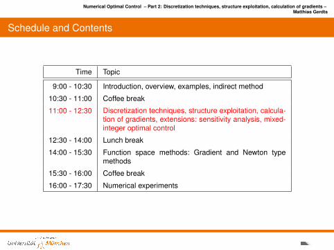
Schedule and Contents
Time Topic
9:00 - 10:30 Introduction, overview, examples, indirect method
10:30 - 11:00 Coffee break
11:00 - 12:30 Discretization techniques, structure exploitation, calcula-tion of gradients, extensions: sensitivity analysis, mixed-integer optimal control
12:30 - 14:00 Lunch break
14:00 - 15:30 Function space methods: Gradient and Newton typemethods
15:30 - 16:00 Coffee break
16:00 - 17:30 Numerical experiments
Numerical Optimal Control – Part 2: Discretization techniques, structure exploitation, calculation of gradients –Matthias Gerdts
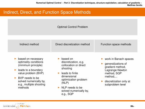
Indirect, Direct, and Function Space Methods
Optimal Control Problem
Indirect method
I based on necessaryoptimality conditions(minimum principle)
I leads to a boundaryvalue problem (BVP)
I BVP needs to besolved numerically by,e.g., multiple shootingmethods
Direct discretization method
I based ondiscretization, e.g.collocation or directshooting
I leads to finitedimensionaloptimization problem(NLP)
I NLP needs to besolved numerically by,e.g., SQP
Function space methods
I work in Banach spacesI generalizations of
gradient method,Lagrange-Newtonmethod, SQPmethod,...
I discretization only atsubproblem level
Numerical Optimal Control – Part 2: Discretization techniques, structure exploitation, calculation of gradients –Matthias Gerdts
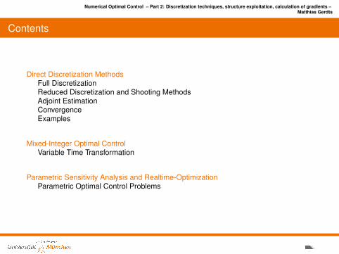
Contents
Direct Discretization MethodsFull DiscretizationReduced Discretization and Shooting MethodsAdjoint EstimationConvergenceExamples
Mixed-Integer Optimal ControlVariable Time Transformation
Parametric Sensitivity Analysis and Realtime-OptimizationParametric Optimal Control Problems
Numerical Optimal Control – Part 2: Discretization techniques, structure exploitation, calculation of gradients –Matthias Gerdts
Optimal Control Problem
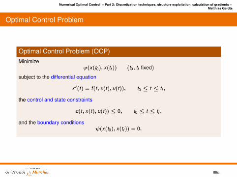
Optimal Control Problem (OCP)Minimize
ϕ(x(t0), x(tf )) (t0, tf fixed)
subject to the differential equation
x′(t) = f (t, x(t), u(t)), t0 ≤ t ≤ tf ,
the control and state constraints
c(t, x(t), u(t)) ≤ 0, t0 ≤ t ≤ tf ,
and the boundary conditionsψ(x(t0), x(tf )) = 0.
Numerical Optimal Control – Part 2: Discretization techniques, structure exploitation, calculation of gradients –Matthias Gerdts
Direct Discretization Idea
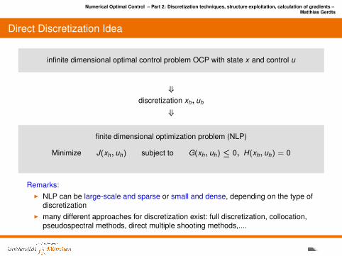
infinite dimensional optimal control problem OCP with state x and control u
⇓discretization xh, uh
⇓
finite dimensional optimization problem (NLP)
Minimize J(xh, uh) subject to G(xh, uh) ≤ 0, H(xh, uh) = 0
Remarks:I NLP can be large-scale and sparse or small and dense, depending on the type of
discretizationI many different approaches for discretization exist: full discretization, collocation,
pseudospectral methods, direct multiple shooting methods,....
Numerical Optimal Control – Part 2: Discretization techniques, structure exploitation, calculation of gradients –Matthias Gerdts
Direct Discretization Idea
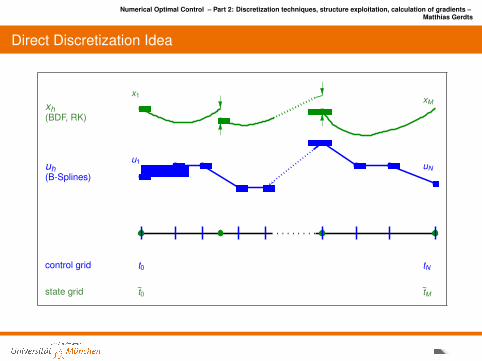
control grid t0 tN
u1 uNuh(B-Splines)
state grid t0 tM
x1 xMxh(BDF, RK)
Numerical Optimal Control – Part 2: Discretization techniques, structure exploitation, calculation of gradients –Matthias Gerdts
State Discretization
Throughout we use one-step methods for the discretization of the differential equation
x′(t) = f (t, x(t), u(t))
on a grid (equidistant for simplicity)
Gh := ti := t0 + ih; | i = 0, 1, . . . ,N, h =tf − t0
N, N ∈ N
One-step MethodsThe one-step method is defined by the recursion
xi+1 = xi + hΦ(ti , xi , uh, h), i = 0, 1, . . . ,N − 1,
and provides approximations xi = xh(ti ) ≈ x(ti ) at ti ∈ Gh.The function Φ is called increment function. It depends on uh, which represents acontrol parameterization to be discussed later.
Remark:I The control approximation uh needs to be defined. There are different ways to do
it; all of them lead to different discretization schemes for OCP.
Numerical Optimal Control – Part 2: Discretization techniques, structure exploitation, calculation of gradients –Matthias Gerdts
State Discretization
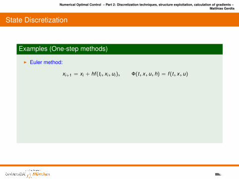
Examples (One-step methods)
I Euler method:
xi+1 = xi + hf (ti , xi , ui ), Φ(t, x, u, h) = f (t, x, u)
I Heun’s method: “stage derivatives”
k1 = f (ti , xi , )
k2 = f (ti + h, xi + hk1, )
xi+1 = xi +h2
(k1 + k2)
Numerical Optimal Control – Part 2: Discretization techniques, structure exploitation, calculation of gradients –Matthias Gerdts
State Discretization
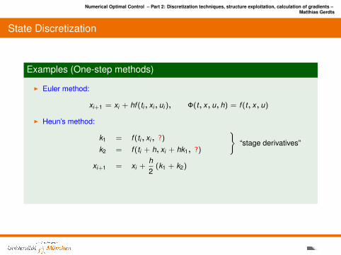
Examples (One-step methods)
I Euler method:
xi+1 = xi + hf (ti , xi , ui ), Φ(t, x, u, h) = f (t, x, u)
I Heun’s method: “stage derivatives”
k1 = f (ti , xi , ?)
k2 = f (ti + h, xi + hk1, ?)
xi+1 = xi +h2
(k1 + k2)

Numerical Optimal Control – Part 2: Discretization techniques, structure exploitation, calculation of gradients –Matthias Gerdts
State Discretization
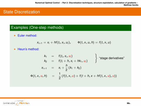
Examples (One-step methods)
I Euler method:
xi+1 = xi + hf (ti , xi , ui ), Φ(t, x, u, h) = f (t, x, u)
I Heun’s method: “stage derivatives”
k1 = f (ti , xi , ui )
k2 = f (ti + h, xi + hk1, ui )
xi+1 = xi +h2
(k1 + k2)
Numerical Optimal Control – Part 2: Discretization techniques, structure exploitation, calculation of gradients –Matthias Gerdts
State Discretization
Examples (One-step methods)
I Euler method:
xi+1 = xi + hf (ti , xi , ui ), Φ(t, x, u, h) = f (t, x, u)
I Heun’s method: “stage derivatives”
k1 = f (ti , xi , ui )
k2 = f (ti + h, xi + hk1, ui )
xi+1 = xi +h2
(k1 + k2)
Φ(t, x, u, h) =12
(f (t, x, u) + f (t + h, x + hf (t, x, u), u))

Numerical Optimal Control – Part 2: Discretization techniques, structure exploitation, calculation of gradients –Matthias Gerdts
State Discretization
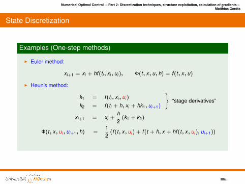
Examples (One-step methods)
I Euler method:
xi+1 = xi + hf (ti , xi , ui ), Φ(t, x, u, h) = f (t, x, u)
I Heun’s method: “stage derivatives”
k1 = f (ti , xi , ui )
k2 = f (ti + h, xi + hk1, ui+1)
xi+1 = xi +h2
(k1 + k2)
Numerical Optimal Control – Part 2: Discretization techniques, structure exploitation, calculation of gradients –Matthias Gerdts
State Discretization
Examples (One-step methods)
I Euler method:
xi+1 = xi + hf (ti , xi , ui ), Φ(t, x, u, h) = f (t, x, u)
I Heun’s method: “stage derivatives”
k1 = f (ti , xi , ui )
k2 = f (ti + h, xi + hk1, ui+1)
xi+1 = xi +h2
(k1 + k2)
Φ(t, x, ui , ui+1, h) =12
(f (t, x, ui ) + f (t + h, x + hf (t, x, ui ), ui+1))

Numerical Optimal Control – Part 2: Discretization techniques, structure exploitation, calculation of gradients –Matthias Gerdts
State Discretization
Examples (One-step methods)
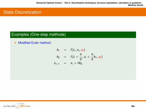
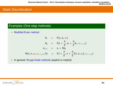
I Modified Euler method:
k1 = f (ti , xi , ?)
k2 = f (ti +h2, xi +
h2
k1, ?)
xi+1 = xi + hk2
I In general: Runge-Kutta methods (explicit or implicit)
Numerical Optimal Control – Part 2: Discretization techniques, structure exploitation, calculation of gradients –Matthias Gerdts
State Discretization
Examples (One-step methods)
I Modified Euler method:
k1 = f (ti , xi , ui )
k2 = f (ti +h2, xi +
h2
k1, ui )
xi+1 = xi + hk2
I In general: Runge-Kutta methods (explicit or implicit)
Numerical Optimal Control – Part 2: Discretization techniques, structure exploitation, calculation of gradients –Matthias Gerdts
State Discretization
Examples (One-step methods)
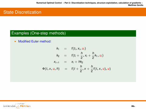
I Modified Euler method:
k1 = f (ti , xi , ui )
k2 = f (ti +h2, xi +
h2
k1, ui )
xi+1 = xi + hk2
Φ(t, x, u, h) = f (t +h2, x +
h2
f (t, x, u), u)
I In general: Runge-Kutta methods (explicit or implicit)
Numerical Optimal Control – Part 2: Discretization techniques, structure exploitation, calculation of gradients –Matthias Gerdts
State Discretization
Examples (One-step methods)
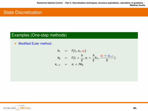
I Modified Euler method:
k1 = f (ti , xi , ui )
k2 = f (ti +h2, xi +
h2
k1,ui + ui+1
2)
xi+1 = xi + hk2
I In general: Runge-Kutta methods (explicit or implicit)
Numerical Optimal Control – Part 2: Discretization techniques, structure exploitation, calculation of gradients –Matthias Gerdts
State Discretization
Examples (One-step methods)
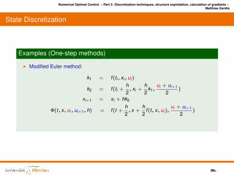
I Modified Euler method:
k1 = f (ti , xi , ui )
k2 = f (ti +h2, xi +
h2
k1,ui + ui+1
2)
xi+1 = xi + hk2
Φ(t, x, ui , ui+1, h) = f (t +h2, x +
h2
f (t, x, ui ),ui + ui+1
2)
I In general: Runge-Kutta methods (explicit or implicit)

Numerical Optimal Control – Part 2: Discretization techniques, structure exploitation, calculation of gradients –Matthias Gerdts
State Discretization
Examples (One-step methods)
I Modified Euler method:
k1 = f (ti , xi , ui )
k2 = f (ti +h2, xi +
h2
k1, ui+1/2)
xi+1 = xi + hk2
Φ(t, x, ui , ui+1/2, h) = f (t +h2, x +
h2
f (t, x, ui ), ui+1/2)
I In general: Runge-Kutta methods (explicit or implicit)
Numerical Optimal Control – Part 2: Discretization techniques, structure exploitation, calculation of gradients –Matthias Gerdts
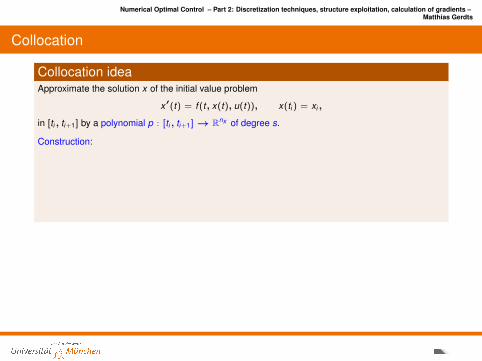
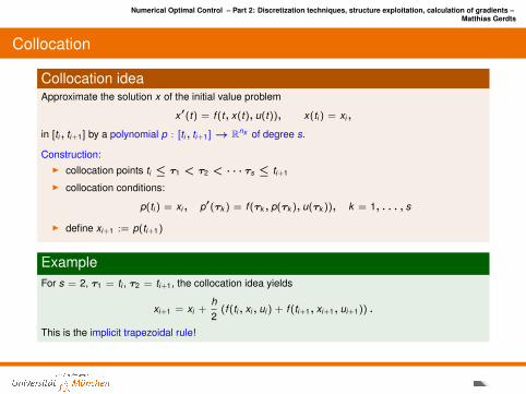
Collocation
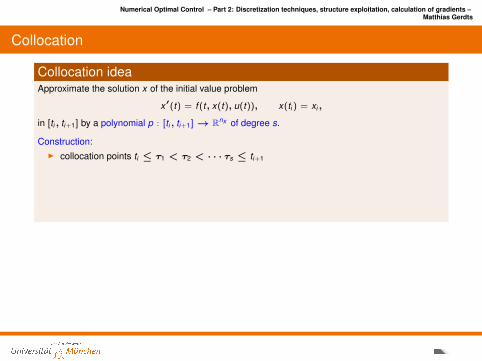
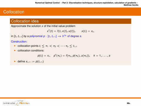
Collocation ideaApproximate the solution x of the initial value problem
x′(t) = f (t, x(t), u(t)), x(ti ) = xi ,
in [ti , ti+1] by a polynomial p : [ti , ti+1]→ Rnx of degree s.
Construction:
I collocation points ti ≤ τ1 < τ2 < · · · τs ≤ ti+1
I collocation conditions:
p(ti ) = xi , p′(τk ) = f (τk , p(τk ), u(τk )), k = 1, . . . , s
I define xi+1 := p(ti+1)
ExampleFor s = 2, τ1 = ti , τ2 = ti+1, the collocation idea yields
xi+1 = xi +h2
(f (ti , xi , ui ) + f (ti+1, xi+1, ui+1)) .
This is the implicit trapezoidal rule!
In general: Every collocation method corresponds to an implicit Runge-Kutta method.
Numerical Optimal Control – Part 2: Discretization techniques, structure exploitation, calculation of gradients –Matthias Gerdts
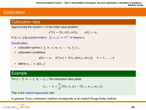
Collocation
Collocation ideaApproximate the solution x of the initial value problem
x′(t) = f (t, x(t), u(t)), x(ti ) = xi ,
in [ti , ti+1] by a polynomial p : [ti , ti+1]→ Rnx of degree s.
Construction:I collocation points ti ≤ τ1 < τ2 < · · · τs ≤ ti+1
I collocation conditions:
p(ti ) = xi , p′(τk ) = f (τk , p(τk ), u(τk )), k = 1, . . . , s
I define xi+1 := p(ti+1)
ExampleFor s = 2, τ1 = ti , τ2 = ti+1, the collocation idea yields
xi+1 = xi +h2
(f (ti , xi , ui ) + f (ti+1, xi+1, ui+1)) .
This is the implicit trapezoidal rule!
In general: Every collocation method corresponds to an implicit Runge-Kutta method.

Numerical Optimal Control – Part 2: Discretization techniques, structure exploitation, calculation of gradients –Matthias Gerdts
Collocation
Collocation ideaApproximate the solution x of the initial value problem
x′(t) = f (t, x(t), u(t)), x(ti ) = xi ,
in [ti , ti+1] by a polynomial p : [ti , ti+1]→ Rnx of degree s.
Construction:I collocation points ti ≤ τ1 < τ2 < · · · τs ≤ ti+1
I collocation conditions:
p(ti ) = xi , p′(τk ) = f (τk , p(τk ), u(τk )), k = 1, . . . , s
I define xi+1 := p(ti+1)
ExampleFor s = 2, τ1 = ti , τ2 = ti+1, the collocation idea yields
xi+1 = xi +h2
(f (ti , xi , ui ) + f (ti+1, xi+1, ui+1)) .
This is the implicit trapezoidal rule!
In general: Every collocation method corresponds to an implicit Runge-Kutta method.
Numerical Optimal Control – Part 2: Discretization techniques, structure exploitation, calculation of gradients –Matthias Gerdts
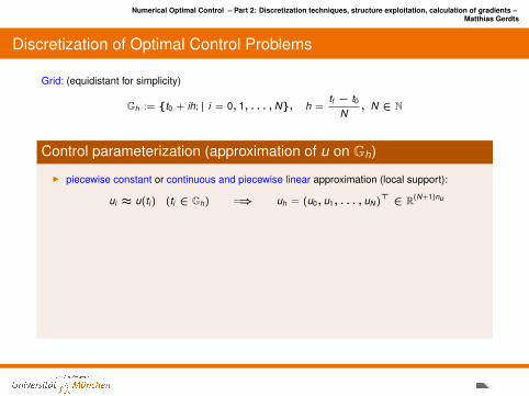
Discretization of Optimal Control Problems
Grid: (equidistant for simplicity)
Gh := t0 + ih; | i = 0, 1, . . . , N, h =tf − t0
N, N ∈ N
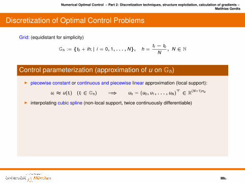
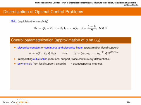
Control parameterization (approximation of u on Gh)
I piecewise constant or continuous and piecewise linear approximation (local support):
ui ≈ u(ti ) (ti ∈ Gh) =⇒ uh = (u0, u1, . . . , uN )> ∈ R(N+1)nu
I interpolating cubic spline (non-local support, twice continuously differentiable)I polynomials (non-local support, smooth)−→ pseudospectral methodsI B-spline approximations of order k (local support, arbitrary smoothness possible):
uh(t) = uh(t ; w) :=
N+k−1∑i=1
wi Bki (t), w = (w1, . . . , wM )> ∈ RMnu ,M := N + k − 1
Bki : basis functions (elementary B-splines); w : control parameterization
Numerical Optimal Control – Part 2: Discretization techniques, structure exploitation, calculation of gradients –Matthias Gerdts
Discretization of Optimal Control Problems
Grid: (equidistant for simplicity)
Gh := t0 + ih; | i = 0, 1, . . . , N, h =tf − t0
N, N ∈ N
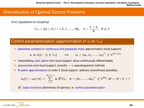
Control parameterization (approximation of u on Gh)
I piecewise constant or continuous and piecewise linear approximation (local support):
ui ≈ u(ti ) (ti ∈ Gh) =⇒ uh = (u0, u1, . . . , uN )> ∈ R(N+1)nu
I interpolating cubic spline (non-local support, twice continuously differentiable)
I polynomials (non-local support, smooth)−→ pseudospectral methodsI B-spline approximations of order k (local support, arbitrary smoothness possible):
uh(t) = uh(t ; w) :=
N+k−1∑i=1
wi Bki (t), w = (w1, . . . , wM )> ∈ RMnu ,M := N + k − 1
Bki : basis functions (elementary B-splines); w : control parameterization
Numerical Optimal Control – Part 2: Discretization techniques, structure exploitation, calculation of gradients –Matthias Gerdts
Discretization of Optimal Control Problems
Grid: (equidistant for simplicity)
Gh := t0 + ih; | i = 0, 1, . . . , N, h =tf − t0
N, N ∈ N
Control parameterization (approximation of u on Gh)
I piecewise constant or continuous and piecewise linear approximation (local support):
ui ≈ u(ti ) (ti ∈ Gh) =⇒ uh = (u0, u1, . . . , uN )> ∈ R(N+1)nu
I interpolating cubic spline (non-local support, twice continuously differentiable)I polynomials (non-local support, smooth)−→ pseudospectral methods
I B-spline approximations of order k (local support, arbitrary smoothness possible):
uh(t) = uh(t ; w) :=
N+k−1∑i=1
wi Bki (t), w = (w1, . . . , wM )> ∈ RMnu ,M := N + k − 1
Bki : basis functions (elementary B-splines); w : control parameterization
Numerical Optimal Control – Part 2: Discretization techniques, structure exploitation, calculation of gradients –Matthias Gerdts
Discretization of Optimal Control Problems
Grid: (equidistant for simplicity)
Gh := t0 + ih; | i = 0, 1, . . . , N, h =tf − t0
N, N ∈ N
Control parameterization (approximation of u on Gh)
I piecewise constant or continuous and piecewise linear approximation (local support):
ui ≈ u(ti ) (ti ∈ Gh) =⇒ uh = (u0, u1, . . . , uN )> ∈ R(N+1)nu
I interpolating cubic spline (non-local support, twice continuously differentiable)I polynomials (non-local support, smooth)−→ pseudospectral methodsI B-spline approximations of order k (local support, arbitrary smoothness possible):
uh(t) = uh(t ; w) :=
N+k−1∑i=1
wi Bki (t), w = (w1, . . . , wM )> ∈ RMnu ,M := N + k − 1
Bki : basis functions (elementary B-splines); w : control parameterization
Numerical Optimal Control – Part 2: Discretization techniques, structure exploitation, calculation of gradients –Matthias Gerdts
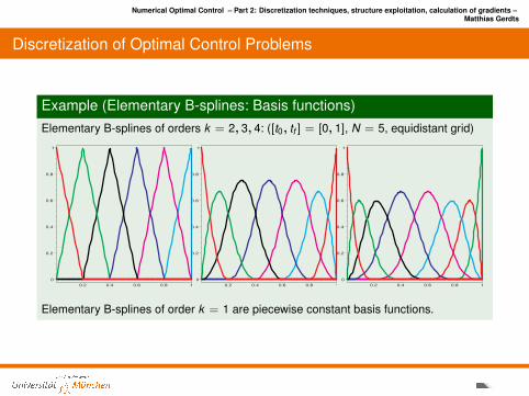
Discretization of Optimal Control Problems
Example (Elementary B-splines: Basis functions)Elementary B-splines of orders k = 2, 3, 4: ([t0, tf ] = [0, 1], N = 5, equidistant grid)
0
0.2
0.4
0.6
0.8
1
0.2 0.4 0.6 0.8 1
0
0.2
0.4
0.6
0.8
1
0.2 0.4 0.6 0.8 1
0
0.2
0.4
0.6
0.8
1
0.2 0.4 0.6 0.8 1
Elementary B-splines of order k = 1 are piecewise constant basis functions.
Numerical Optimal Control – Part 2: Discretization techniques, structure exploitation, calculation of gradients –Matthias Gerdts
Discretization of Optimal Control Problems
Definition (elementary B-Spline of order k )Let k ∈ N. Define the auxiliary grid
Gkh := τi | i = 1, . . . , N + 2k − 1
with auxiliary grid points
τi :=
t0, if 1 ≤ i ≤ k,
ti−k , if k + 1 ≤ i ≤ N + k − 1,
tN , if N + k ≤ i ≤ N + 2k − 1.
The elementary B-splines Bki (·) of order k for i = 1, . . . , N + k − 1 are defined by the recursion
B1i (t) :=
1, if τi ≤ t < τi+1
0, otherwise(“piecewise constant”)
Bki (t) :=
t − τi
τi+k−1 − τiBk−1
i (t) +τi+k − tτi+k − τi+1
Bk−1i+1 (t)
convention: 0/0 = 0 whenever auxiliary grid points coincide.
Numerical Optimal Control – Part 2: Discretization techniques, structure exploitation, calculation of gradients –Matthias Gerdts
Discretization of Optimal Control Problems
Example
I For k = 2 we obtain the continuous and piecewise linear functions
B2i (t) =
t−τiτi+1−τi
, if τi ≤ t < τi+1,
τi+2−tτi+2−τi+1
, if τi+1 ≤ t < τi+2,
0, otherwise.
I For k = 3 we obtain the continuously differentiable function
B3i (t) =
(t−τi )2
(τi+2−τi )(τi+1−τi ) , if t ∈ [τi , τi+1),
(t−τi )(τi+2−t)(τi+2−τi )(τi+2−τi+1) +
(τi+3−t)(t−τi+1)
(τi+3−τi+1)(τi+2−τi+1) , if t ∈ [τi+1, τi+2),
(τi+3−t)2
(τi+3−τi+1)(τi+3−τi+2) , if t ∈ [τi+2, τi+3),
0, otherwise.
Numerical Optimal Control – Part 2: Discretization techniques, structure exploitation, calculation of gradients –Matthias Gerdts
Discretization of Optimal Control Problems
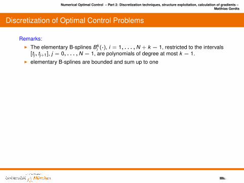
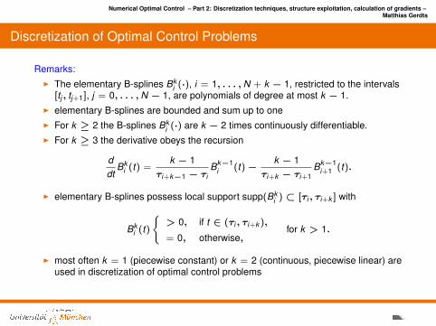
Remarks:I The elementary B-splines Bk
i (·), i = 1, . . . ,N + k − 1, restricted to the intervals[tj , tj+1], j = 0, . . . ,N − 1, are polynomials of degree at most k − 1.
I elementary B-splines are bounded and sum up to oneI For k ≥ 2 the B-splines Bk
i (·) are k − 2 times continuously differentiable.I For k ≥ 3 the derivative obeys the recursion
ddt
Bki (t) =
k − 1τi+k−1 − τi
Bk−1i (t)−
k − 1τi+k − τi+1
Bk−1i+1 (t).
I elementary B-splines possess local support supp(Bki ) ⊂ [τi , τi+k ] with
Bki (t)
> 0, if t ∈ (τi , τi+k ),
= 0, otherwise,for k > 1.
I most often k = 1 (piecewise constant) or k = 2 (continuous, piecewise linear) areused in discretization of optimal control problems
Numerical Optimal Control – Part 2: Discretization techniques, structure exploitation, calculation of gradients –Matthias Gerdts
Discretization of Optimal Control Problems
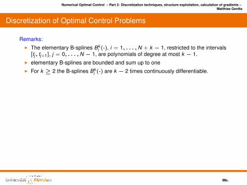
Remarks:I The elementary B-splines Bk
i (·), i = 1, . . . ,N + k − 1, restricted to the intervals[tj , tj+1], j = 0, . . . ,N − 1, are polynomials of degree at most k − 1.
I elementary B-splines are bounded and sum up to one
I For k ≥ 2 the B-splines Bki (·) are k − 2 times continuously differentiable.
I For k ≥ 3 the derivative obeys the recursion
ddt
Bki (t) =
k − 1τi+k−1 − τi
Bk−1i (t)−
k − 1τi+k − τi+1
Bk−1i+1 (t).
I elementary B-splines possess local support supp(Bki ) ⊂ [τi , τi+k ] with
Bki (t)
> 0, if t ∈ (τi , τi+k ),
= 0, otherwise,for k > 1.
I most often k = 1 (piecewise constant) or k = 2 (continuous, piecewise linear) areused in discretization of optimal control problems
Numerical Optimal Control – Part 2: Discretization techniques, structure exploitation, calculation of gradients –Matthias Gerdts
Discretization of Optimal Control Problems
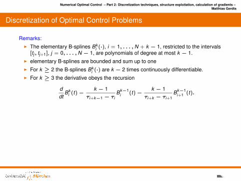
Remarks:I The elementary B-splines Bk
i (·), i = 1, . . . ,N + k − 1, restricted to the intervals[tj , tj+1], j = 0, . . . ,N − 1, are polynomials of degree at most k − 1.
I elementary B-splines are bounded and sum up to oneI For k ≥ 2 the B-splines Bk
i (·) are k − 2 times continuously differentiable.
I For k ≥ 3 the derivative obeys the recursion
ddt
Bki (t) =
k − 1τi+k−1 − τi
Bk−1i (t)−
k − 1τi+k − τi+1
Bk−1i+1 (t).
I elementary B-splines possess local support supp(Bki ) ⊂ [τi , τi+k ] with
Bki (t)
> 0, if t ∈ (τi , τi+k ),
= 0, otherwise,for k > 1.
I most often k = 1 (piecewise constant) or k = 2 (continuous, piecewise linear) areused in discretization of optimal control problems
Numerical Optimal Control – Part 2: Discretization techniques, structure exploitation, calculation of gradients –Matthias Gerdts
Discretization of Optimal Control Problems
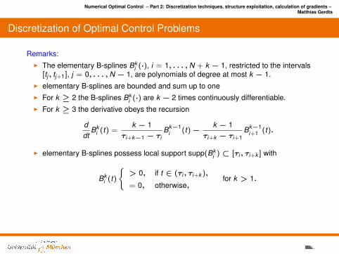
Remarks:I The elementary B-splines Bk
i (·), i = 1, . . . ,N + k − 1, restricted to the intervals[tj , tj+1], j = 0, . . . ,N − 1, are polynomials of degree at most k − 1.
I elementary B-splines are bounded and sum up to oneI For k ≥ 2 the B-splines Bk
i (·) are k − 2 times continuously differentiable.I For k ≥ 3 the derivative obeys the recursion
ddt
Bki (t) =
k − 1τi+k−1 − τi
Bk−1i (t)−
k − 1τi+k − τi+1
Bk−1i+1 (t).
I elementary B-splines possess local support supp(Bki ) ⊂ [τi , τi+k ] with
Bki (t)
> 0, if t ∈ (τi , τi+k ),
= 0, otherwise,for k > 1.
I most often k = 1 (piecewise constant) or k = 2 (continuous, piecewise linear) areused in discretization of optimal control problems
Numerical Optimal Control – Part 2: Discretization techniques, structure exploitation, calculation of gradients –Matthias Gerdts
Discretization of Optimal Control Problems
Remarks:I The elementary B-splines Bk
i (·), i = 1, . . . ,N + k − 1, restricted to the intervals[tj , tj+1], j = 0, . . . ,N − 1, are polynomials of degree at most k − 1.
I elementary B-splines are bounded and sum up to oneI For k ≥ 2 the B-splines Bk
i (·) are k − 2 times continuously differentiable.I For k ≥ 3 the derivative obeys the recursion
ddt
Bki (t) =
k − 1τi+k−1 − τi
Bk−1i (t)−
k − 1τi+k − τi+1
Bk−1i+1 (t).
I elementary B-splines possess local support supp(Bki ) ⊂ [τi , τi+k ] with
Bki (t)
> 0, if t ∈ (τi , τi+k ),
= 0, otherwise,for k > 1.
I most often k = 1 (piecewise constant) or k = 2 (continuous, piecewise linear) areused in discretization of optimal control problems
Numerical Optimal Control – Part 2: Discretization techniques, structure exploitation, calculation of gradients –Matthias Gerdts
Contents
Direct Discretization MethodsFull DiscretizationReduced Discretization and Shooting MethodsAdjoint EstimationConvergenceExamples
Mixed-Integer Optimal ControlVariable Time Transformation
Parametric Sensitivity Analysis and Realtime-OptimizationParametric Optimal Control Problems
Numerical Optimal Control – Part 2: Discretization techniques, structure exploitation, calculation of gradients –Matthias Gerdts
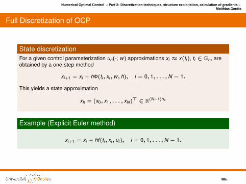
Full Discretization of OCP
State discretizationFor a given control parameterization uh(·; w) approximations xi ≈ x(ti ), ti ∈ Gh, areobtained by a one-step method
xi+1 = xi + hΦ(ti , xi ,w, h), i = 0, 1, . . . ,N − 1.
This yields a state approximation
xh = (x0, x1, . . . , xN )> ∈ R(N+1)nx
Example (Explicit Euler method)
xi+1 = xi + hf (ti , xi , ui ), i = 0, 1, . . . ,N − 1.
Numerical Optimal Control – Part 2: Discretization techniques, structure exploitation, calculation of gradients –Matthias Gerdts
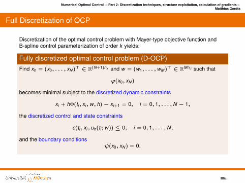
Full Discretization of OCP
Discretization of the optimal control problem with Mayer-type objective function andB-spline control parameterization of order k yields:
Fully discretized optimal control problem (D-OCP)Find xh = (x0, . . . , xN )> ∈ R(N+1)nx and w = (w1, . . . ,wM )> ∈ RMnu such that
ϕ(x0, xN )
becomes minimal subject to the discretized dynamic constraints
xi + hΦ(ti , xi ,w, h)− xi+1 = 0, i = 0, 1, . . . ,N − 1,
the discretized control and state constraints
c(ti , xi , uh(ti ; w)) ≤ 0, i = 0, 1, . . . ,N,
and the boundary conditionsψ(x0, xN ) = 0.
Numerical Optimal Control – Part 2: Discretization techniques, structure exploitation, calculation of gradients –Matthias Gerdts
Full Discretization of OCP
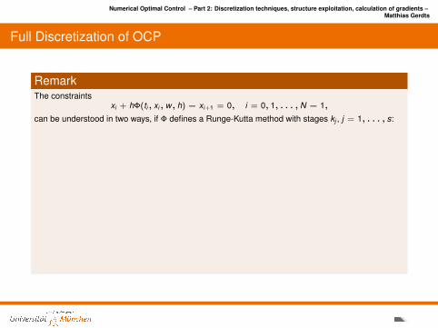
RemarkThe constraints
xi + hΦ(ti , xi , w, h)− xi+1 = 0, i = 0, 1, . . . , N − 1,
can be understood in two ways, if Φ defines a Runge-Kutta method with stages kj , j = 1, . . . , s:
I The stage equations kj = . . . are not explicitly added as equality constraints in D-OCP, e.g.for Heun’s method one would only add the constraints
xi +h2
(f (ti , xi , ui ) + f (ti+1, xi + hf (ti , xi , ui ), ui ))− xi+1 = 0
I The stage equations kj = . . . are explicitly added as equality constraints in D-OCP, e.g. forHeun’s method one would add the constraints
k1 − f (ti , xi , ui ) = 0
k2 − f (ti+1, xi + hk1, ui ) = 0
xi +h2
(k1 + k2)− xi+1 = 0
This version is typically implemented for implicit Runge-Kutta methods.
Numerical Optimal Control – Part 2: Discretization techniques, structure exploitation, calculation of gradients –Matthias Gerdts
Full Discretization of OCP
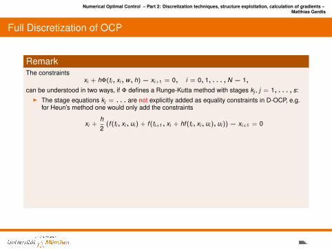
RemarkThe constraints
xi + hΦ(ti , xi , w, h)− xi+1 = 0, i = 0, 1, . . . , N − 1,
can be understood in two ways, if Φ defines a Runge-Kutta method with stages kj , j = 1, . . . , s:I The stage equations kj = . . . are not explicitly added as equality constraints in D-OCP, e.g.
for Heun’s method one would only add the constraints
xi +h2
(f (ti , xi , ui ) + f (ti+1, xi + hf (ti , xi , ui ), ui ))− xi+1 = 0
I The stage equations kj = . . . are explicitly added as equality constraints in D-OCP, e.g. forHeun’s method one would add the constraints
k1 − f (ti , xi , ui ) = 0
k2 − f (ti+1, xi + hk1, ui ) = 0
xi +h2
(k1 + k2)− xi+1 = 0
This version is typically implemented for implicit Runge-Kutta methods.
Numerical Optimal Control – Part 2: Discretization techniques, structure exploitation, calculation of gradients –Matthias Gerdts
Full Discretization of OCP
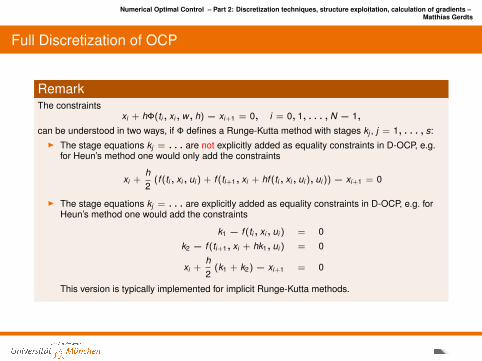
RemarkThe constraints
xi + hΦ(ti , xi , w, h)− xi+1 = 0, i = 0, 1, . . . , N − 1,
can be understood in two ways, if Φ defines a Runge-Kutta method with stages kj , j = 1, . . . , s:I The stage equations kj = . . . are not explicitly added as equality constraints in D-OCP, e.g.
for Heun’s method one would only add the constraints
xi +h2
(f (ti , xi , ui ) + f (ti+1, xi + hf (ti , xi , ui ), ui ))− xi+1 = 0
I The stage equations kj = . . . are explicitly added as equality constraints in D-OCP, e.g. forHeun’s method one would add the constraints
k1 − f (ti , xi , ui ) = 0
k2 − f (ti+1, xi + hk1, ui ) = 0
xi +h2
(k1 + k2)− xi+1 = 0
This version is typically implemented for implicit Runge-Kutta methods.
Numerical Optimal Control – Part 2: Discretization techniques, structure exploitation, calculation of gradients –Matthias Gerdts
Full Discretization of OCP
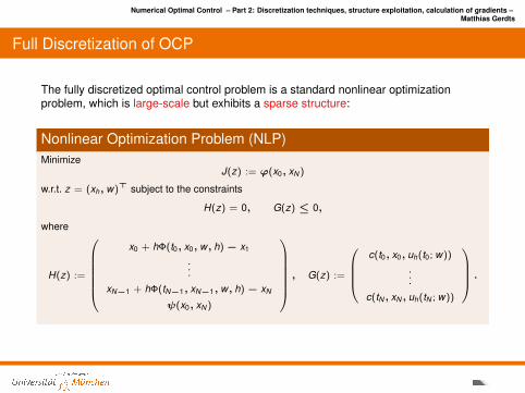
The fully discretized optimal control problem is a standard nonlinear optimizationproblem, which is large-scale but exhibits a sparse structure:
Nonlinear Optimization Problem (NLP)Minimize
J(z) := ϕ(x0, xN )
w.r.t. z = (xh, w)> subject to the constraints
H(z) = 0, G(z) ≤ 0,
where
H(z) :=
x0 + hΦ(t0, x0, w, h)− x1
...
xN−1 + hΦ(tN−1, xN−1, w, h)− xN
ψ(x0, xN )
, G(z) :=
c(t0, x0, uh(t0; w))
...
c(tN , xN , uh(tN ; w))
.
Numerical Optimal Control – Part 2: Discretization techniques, structure exploitation, calculation of gradients –Matthias Gerdts
Sparsity Structures in D-OCP
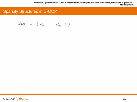
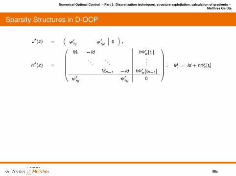
J′(z) =(ϕ′x0
ϕ′xN0),
H′(z) =
M0 −Id hΦ′w [t0]
. . .. . .
...
MN−1 −Id hΦ′w [tN−1]
ψ′x0ψ′xN
0
, Mj := Id + hΦ′x [tj ]
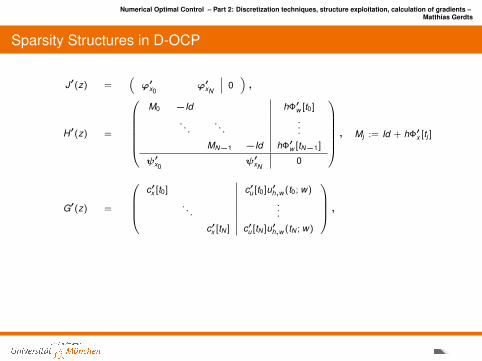
G′(z) =
c′x [t0] c′u [t0]u′h,w (t0; w)
. . ....
c′x [tN ] c′u [tN ]u′h,w (tN ; w)
,
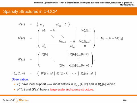
u′h,w (tj ; w) =(
Bk1 (tj ) · Id Bk
2 (tj ) · Id · · · BkM (tj ) · Id
)Observation:
I Bki have local support =⇒ most entries in u′h,w (tj ; w) and in Φ′w [tj ] vanish
I H′(z) and G′(z) have a large-scale and sparse structure.
Numerical Optimal Control – Part 2: Discretization techniques, structure exploitation, calculation of gradients –Matthias Gerdts
Sparsity Structures in D-OCP
J′(z) =(ϕ′x0
ϕ′xN0),
H′(z) =
M0 −Id hΦ′w [t0]
. . .. . .
...
MN−1 −Id hΦ′w [tN−1]
ψ′x0ψ′xN
0
, Mj := Id + hΦ′x [tj ]
G′(z) =
c′x [t0] c′u [t0]u′h,w (t0; w)
. . ....
c′x [tN ] c′u [tN ]u′h,w (tN ; w)
,
u′h,w (tj ; w) =(
Bk1 (tj ) · Id Bk
2 (tj ) · Id · · · BkM (tj ) · Id
)Observation:
I Bki have local support =⇒ most entries in u′h,w (tj ; w) and in Φ′w [tj ] vanish
I H′(z) and G′(z) have a large-scale and sparse structure.
Numerical Optimal Control – Part 2: Discretization techniques, structure exploitation, calculation of gradients –Matthias Gerdts
Sparsity Structures in the Full Discretization Approach
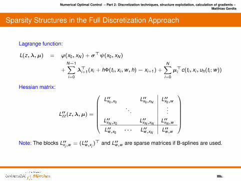
Lagrange function:
L(z, λ, µ) = ϕ(x0, xN ) + σ>ψ(x0, xN )
+
N−1∑i=0
λ>i+1(xi + hΦ(ti , xi ,w, h)− xi+1) +N∑
i=0
µ>i c(ti , xi , uh(ti ; w))
Hessian matrix:
L′′zz (z, λ, µ) =
L′′x0,x0
L′′x0,xNL′′x0,w
. . ....
L′′xN ,x0L′′xN ,xN
L′′xN ,w
L′′w,x0· · · L′′w,xN
L′′w,w
Note: The blocks L′′xj ,w = (L′′w,xj
)> and L′′w,w are sparse matrices if B-splines are used.
Numerical Optimal Control – Part 2: Discretization techniques, structure exploitation, calculation of gradients –Matthias Gerdts
Full Euler Discretization I
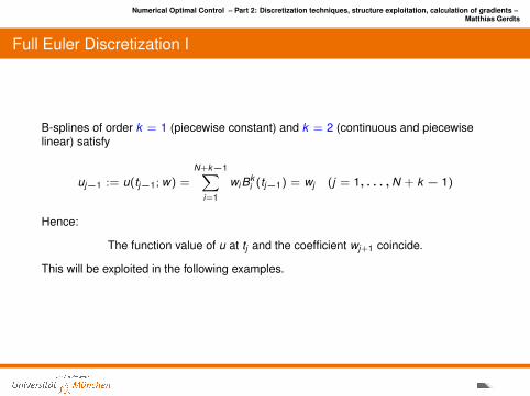
B-splines of order k = 1 (piecewise constant) and k = 2 (continuous and piecewiselinear) satisfy
uj−1 := u(tj−1; w) =
N+k−1∑i=1
wi Bki (tj−1) = wj (j = 1, . . . ,N + k − 1)
Hence:
The function value of u at tj and the coefficient wj+1 coincide.
This will be exploited in the following examples.
Numerical Optimal Control – Part 2: Discretization techniques, structure exploitation, calculation of gradients –Matthias Gerdts
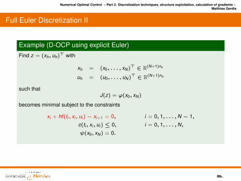
Full Euler Discretization II
Example (D-OCP using explicit Euler)Find z = (xh, uh)> with
xh = (x0, . . . , xN )> ∈ R(N+1)nx
uh = (u0, . . . , uN )> ∈ R(N+1)nu
such thatJ(z) = ϕ(x0, xN )
becomes minimal subject to the constraints
xi + hf (ti , xi , ui )− xi+1 = 0, i = 0, 1, . . . ,N − 1,
c(ti , xi , ui ) ≤ 0, i = 0, 1, . . . ,N,
ψ(x0, xN ) = 0.
Numerical Optimal Control – Part 2: Discretization techniques, structure exploitation, calculation of gradients –Matthias Gerdts
Full Euler Discretization III
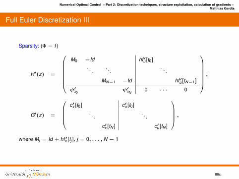
Sparsity: (Φ = f )
H′(z) =
M0 −Id hf ′u [t0]
. . .. . .
. . .
MN−1 −Id hf ′u [tN−1]
ψ′x0ψ′xN
0 · · · 0
,
G′(z) =
c′x [t0] c′u [t0]
. . .. . .
c′x [tN ] c′u [tN ]
,where Mj = Id + hf ′x [tj ], j = 0, . . . ,N − 1
Numerical Optimal Control – Part 2: Discretization techniques, structure exploitation, calculation of gradients –Matthias Gerdts
Full Euler Discretization IV
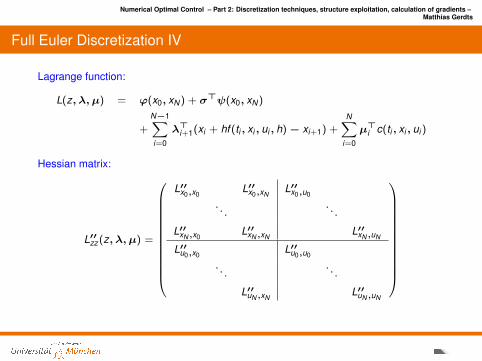
Lagrange function:
L(z, λ, µ) = ϕ(x0, xN ) + σ>ψ(x0, xN )
+
N−1∑i=0
λ>i+1(xi + hf (ti , xi , ui , h)− xi+1) +N∑
i=0
µ>i c(ti , xi , ui )
Hessian matrix:
L′′zz (z, λ, µ) =
L′′x0,x0L′′x0,xN
L′′x0,u0
. . .. . .
L′′xN ,x0L′′xN ,xN
L′′xN ,uN
L′′u0,x0L′′u0,u0
. . .. . .
L′′uN ,xNL′′uN ,uN
Numerical Optimal Control – Part 2: Discretization techniques, structure exploitation, calculation of gradients –Matthias Gerdts
Full Trapezoidal Discretization
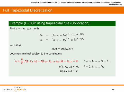
Example (D-OCP using trapezoidal rule (Collocation))Find z = (xh, uh)> with
xh = (x0, . . . , xN )> ∈ R(N+1)nx
uh = (u0, . . . , uN )> ∈ R(N+1)nu
such thatJ(z) = ϕ(x0, xN )
becomes minimal subject to the constraints
xi +h2
(f (ti , xi , ui ) + f (ti+1, xi+1, ui+1))− xi+1 = 0, i = 0, 1, . . . ,N − 1,
c(ti , xi , ui ) ≤ 0, i = 0, 1, . . . ,N,
ψ(x0, xN ) = 0.
Numerical Optimal Control – Part 2: Discretization techniques, structure exploitation, calculation of gradients –Matthias Gerdts
Full Hermite-Simpson Discretization (Collocation) I
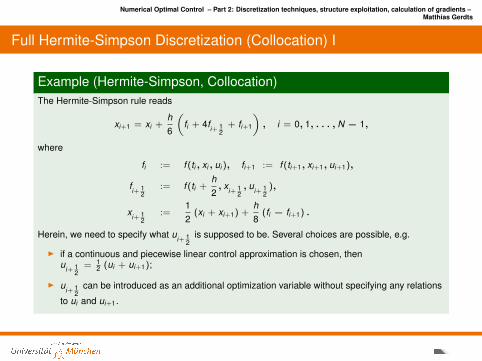
Example (Hermite-Simpson, Collocation)The Hermite-Simpson rule reads
xi+1 = xi +h6
(fi + 4fi+ 1
2+ fi+1
), i = 0, 1, . . . , N − 1,
where
fi := f (ti , xi , ui ), fi+1 := f (ti+1, xi+1, ui+1),
fi+ 12
:= f (ti +h2, xi+ 1
2, ui+ 1
2),
xi+ 12
:=12
(xi + xi+1) +h8
(fi − fi+1) .
Herein, we need to specify what ui+ 12
is supposed to be. Several choices are possible, e.g.
I if a continuous and piecewise linear control approximation is chosen, thenui+ 1
2= 1
2 (ui + ui+1);
I ui+ 12
can be introduced as an additional optimization variable without specifying any relations
to ui and ui+1.
Numerical Optimal Control – Part 2: Discretization techniques, structure exploitation, calculation of gradients –Matthias Gerdts
Full Hermite-Simpson Discretization (Collocation) II
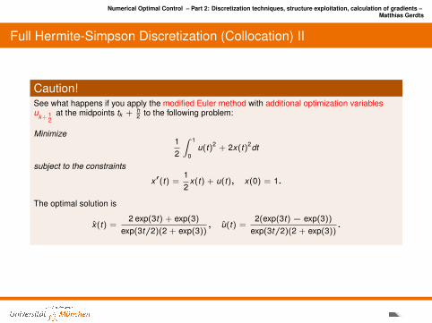
Caution!See what happens if you apply the modified Euler method with additional optimization variablesuk+ 1
2at the midpoints tk + h
2 to the following problem:
Minimize12
∫ 1
0u(t)2 + 2x(t)2dt
subject to the constraints
x′(t) =12
x(t) + u(t), x(0) = 1.
The optimal solution is
x(t) =2 exp(3t) + exp(3)
exp(3t/2)(2 + exp(3)), u(t) =
2(exp(3t)− exp(3))
exp(3t/2)(2 + exp(3)).
Numerical Optimal Control – Part 2: Discretization techniques, structure exploitation, calculation of gradients –Matthias Gerdts
Numerical Solution of D-OCP
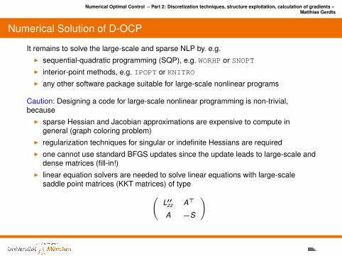
It remains to solve the large-scale and sparse NLP by. e.g.I sequential-quadratic programming (SQP), e.g. WORHP or SNOPTI interior-point methods, e.g. IPOPT or KNITROI any other software package suitable for large-scale nonlinear programs
Caution: Designing a code for large-scale nonlinear programming is non-trivial,because
I sparse Hessian and Jacobian approximations are expensive to compute ingeneral (graph coloring problem)
I regularization techniques for singular or indefinite Hessians are requiredI one cannot use standard BFGS updates since the update leads to large-scale and
dense matrices (fill-in!)I linear equation solvers are needed to solve linear equations with large-scale
saddle point matrices (KKT matrices) of type(L′′zz A>
A −S
)
Numerical Optimal Control – Part 2: Discretization techniques, structure exploitation, calculation of gradients –Matthias Gerdts
Grid Refinement
Approaches:I Refinement based on the local discretization error of the state dynamics and local
refinement at junction points of active/inactive state constraints, see [1, 2]I Refinement taking into account the discretization error in the optimality system
including adjoint equations, see [3]
[1] Betts, J. T. and Huffman, W. P.
Mesh Refinement in Direct Transcription Methods for Optimal Control .
Optimal Control Applications and Methods, 19; 1–21, 1998.
[2] C. Buskens.
Optimierungsmethoden und Sensitivitatsanalyse fur optimale Steuerprozesse mit Steuer- und Zustandsbeschrankungen.
PhD thesis, Fachbereich Mathematik, Westfalische Wilhems-Universitat Munster, Munster, Germany, 1998.
[3] J. Laurent-Varin, F. Bonnans, N. Berend, C. Talbot, and M. Haddou.
On the refinement of discretization for optimal control problems.
IFAC Symposium on Automatic Control in Aerospace, St. Petersburg, 2004.
Numerical Optimal Control – Part 2: Discretization techniques, structure exploitation, calculation of gradients –Matthias Gerdts
Pseudospectral Methods
Approach:I global approximation of control and state by Legendre or Chebyshev polynomialsI direct discretizationI sparse nonlinear programming solver
Advantages:I exponential (or spectral) rate of convergence (faster than polynomial)I good accuracy already with coarse grids
Disadvantages:I oscillations for non-differentiable trajectories
[1] G. Elnagar, M. A. Kazemi, and M. Razzaghi.
The Pseudospectral Legendre Method for Discretizing Optimal Control Problems.
IEEE Transactions on Automatic Control, 40:1793–1796, 1995.
[2] J. Vlassenbroeck and R. Van Doreen.
A Chebyshev Technique for Solving Nonlinear Optimal Control Problems.
IEEE Transactions on Automatic Control, 33:333–340, 1988.
[3] F. Fahroo and I.M. Ross.
Direct Trajectory Optimization by a Chebyshev Pseudospectral Method.
Journal of Guidance Control and Dynamics, 25, 2002.
Numerical Optimal Control – Part 2: Discretization techniques, structure exploitation, calculation of gradients –Matthias Gerdts
Contents
Direct Discretization MethodsFull DiscretizationReduced Discretization and Shooting MethodsAdjoint EstimationConvergenceExamples
Mixed-Integer Optimal ControlVariable Time Transformation
Parametric Sensitivity Analysis and Realtime-OptimizationParametric Optimal Control Problems
Numerical Optimal Control – Part 2: Discretization techniques, structure exploitation, calculation of gradients –Matthias Gerdts
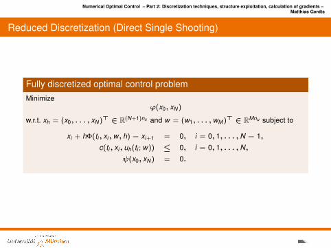
Reduced Discretization (Direct Single Shooting)
Fully discretized optimal control problemMinimize
ϕ(x0, xN )
w.r.t. xh = (x0, . . . , xN )> ∈ R(N+1)nx and w = (w1, . . . ,wM )> ∈ RMnu subject to
xi + hΦ(ti , xi ,w, h)− xi+1 = 0, i = 0, 1, . . . ,N − 1,
c(ti , xi , uh(ti ; w)) ≤ 0, i = 0, 1, . . . ,N,
ψ(x0, xN ) = 0.
Numerical Optimal Control – Part 2: Discretization techniques, structure exploitation, calculation of gradients –Matthias Gerdts
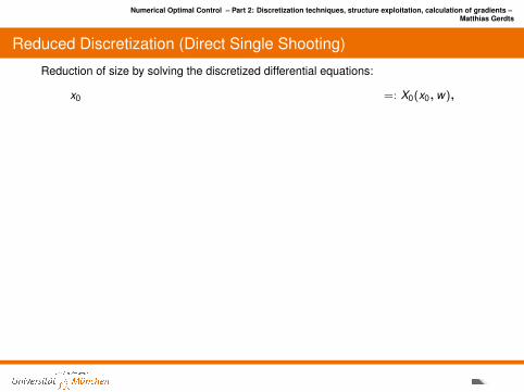
Reduced Discretization (Direct Single Shooting)
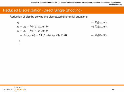
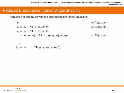
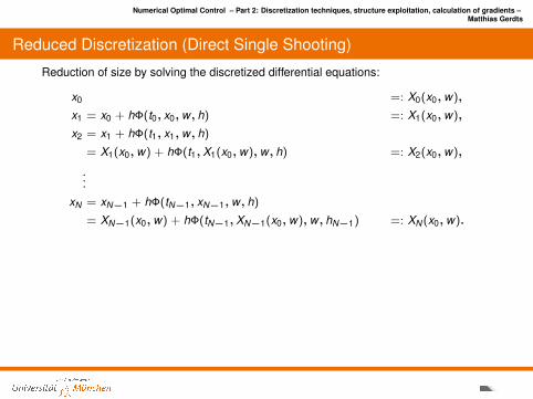
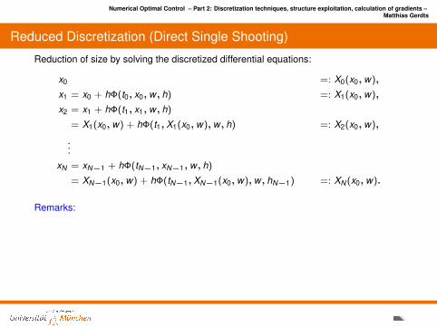
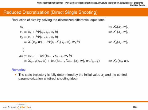
Reduction of size by solving the discretized differential equations:
x0 =: X0(x0,w),
x1 = x0 + hΦ(t0, x0,w, h)
=: X1(x0,w),
x2 = x1 + hΦ(t1, x1,w, h)
= X1(x0,w) + hΦ(t1, X1(x0,w),w, h) =: X2(x0,w),
...
xN = xN−1 + hΦ(tN−1, xN−1,w, h)
= XN−1(x0,w) + hΦ(tN−1, XN−1(x0,w),w, hN−1) =: XN (x0,w).
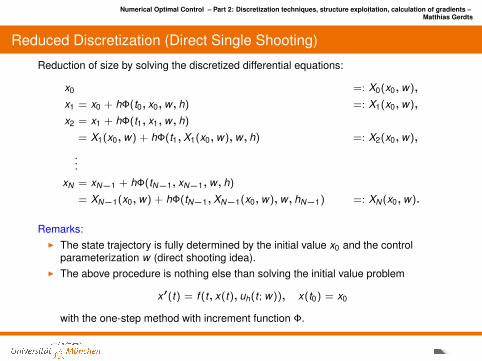
Remarks:I The state trajectory is fully determined by the initial value x0 and the control
parameterization w (direct shooting idea).I The above procedure is nothing else than solving the initial value problem
x′(t) = f (t, x(t), uh(t ; w)), x(t0) = x0
with the one-step method with increment function Φ.
Numerical Optimal Control – Part 2: Discretization techniques, structure exploitation, calculation of gradients –Matthias Gerdts
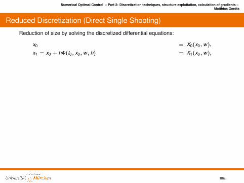
Reduced Discretization (Direct Single Shooting)
Reduction of size by solving the discretized differential equations:
x0 =: X0(x0,w),
x1 = x0 + hΦ(t0, x0,w, h) =: X1(x0,w),
x2 = x1 + hΦ(t1, x1,w, h)
= X1(x0,w) + hΦ(t1, X1(x0,w),w, h) =: X2(x0,w),
...
xN = xN−1 + hΦ(tN−1, xN−1,w, h)
= XN−1(x0,w) + hΦ(tN−1, XN−1(x0,w),w, hN−1) =: XN (x0,w).
Remarks:I The state trajectory is fully determined by the initial value x0 and the control
parameterization w (direct shooting idea).I The above procedure is nothing else than solving the initial value problem
x′(t) = f (t, x(t), uh(t ; w)), x(t0) = x0
with the one-step method with increment function Φ.
Numerical Optimal Control – Part 2: Discretization techniques, structure exploitation, calculation of gradients –Matthias Gerdts
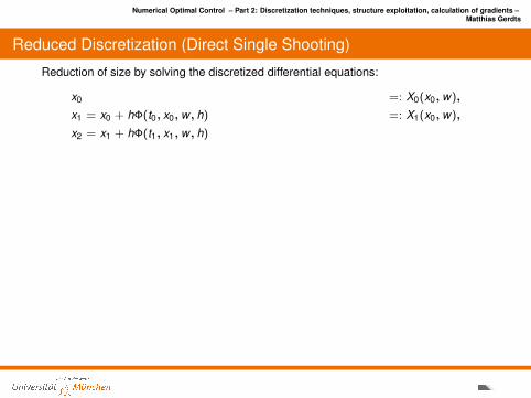
Reduced Discretization (Direct Single Shooting)
Reduction of size by solving the discretized differential equations:
x0 =: X0(x0,w),
x1 = x0 + hΦ(t0, x0,w, h) =: X1(x0,w),
x2 = x1 + hΦ(t1, x1,w, h)
= X1(x0,w) + hΦ(t1, X1(x0,w),w, h) =: X2(x0,w),
...
xN = xN−1 + hΦ(tN−1, xN−1,w, h)
= XN−1(x0,w) + hΦ(tN−1, XN−1(x0,w),w, hN−1) =: XN (x0,w).
Remarks:I The state trajectory is fully determined by the initial value x0 and the control
parameterization w (direct shooting idea).I The above procedure is nothing else than solving the initial value problem
x′(t) = f (t, x(t), uh(t ; w)), x(t0) = x0
with the one-step method with increment function Φ.
Numerical Optimal Control – Part 2: Discretization techniques, structure exploitation, calculation of gradients –Matthias Gerdts
Reduced Discretization (Direct Single Shooting)
Reduction of size by solving the discretized differential equations:
x0 =: X0(x0,w),
x1 = x0 + hΦ(t0, x0,w, h) =: X1(x0,w),
x2 = x1 + hΦ(t1, x1,w, h)
= X1(x0,w) + hΦ(t1, X1(x0,w),w, h) =: X2(x0,w),
...
xN = xN−1 + hΦ(tN−1, xN−1,w, h)
= XN−1(x0,w) + hΦ(tN−1, XN−1(x0,w),w, hN−1) =: XN (x0,w).
Remarks:
I The state trajectory is fully determined by the initial value x0 and the controlparameterization w (direct shooting idea).
I The above procedure is nothing else than solving the initial value problem
x′(t) = f (t, x(t), uh(t ; w)), x(t0) = x0
with the one-step method with increment function Φ.
Numerical Optimal Control – Part 2: Discretization techniques, structure exploitation, calculation of gradients –Matthias Gerdts
Reduced Discretization (Direct Single Shooting)
Reduction of size by solving the discretized differential equations:
x0 =: X0(x0,w),
x1 = x0 + hΦ(t0, x0,w, h) =: X1(x0,w),
x2 = x1 + hΦ(t1, x1,w, h)
= X1(x0,w) + hΦ(t1, X1(x0,w),w, h) =: X2(x0,w),
...
xN = xN−1 + hΦ(tN−1, xN−1,w, h)
= XN−1(x0,w) + hΦ(tN−1, XN−1(x0,w),w, hN−1) =: XN (x0,w).
Remarks:I The state trajectory is fully determined by the initial value x0 and the control
parameterization w (direct shooting idea).
I The above procedure is nothing else than solving the initial value problem
x′(t) = f (t, x(t), uh(t ; w)), x(t0) = x0
with the one-step method with increment function Φ.
Numerical Optimal Control – Part 2: Discretization techniques, structure exploitation, calculation of gradients –Matthias Gerdts
Reduced Discretization (Direct Single Shooting)
Reduction of size by solving the discretized differential equations:
x0 =: X0(x0,w),
x1 = x0 + hΦ(t0, x0,w, h) =: X1(x0,w),
x2 = x1 + hΦ(t1, x1,w, h)
= X1(x0,w) + hΦ(t1, X1(x0,w),w, h) =: X2(x0,w),
...
xN = xN−1 + hΦ(tN−1, xN−1,w, h)
= XN−1(x0,w) + hΦ(tN−1, XN−1(x0,w),w, hN−1) =: XN (x0,w).
Remarks:I The state trajectory is fully determined by the initial value x0 and the control
parameterization w (direct shooting idea).I The above procedure is nothing else than solving the initial value problem
x′(t) = f (t, x(t), uh(t ; w)), x(t0) = x0
with the one-step method with increment function Φ.
Numerical Optimal Control – Part 2: Discretization techniques, structure exploitation, calculation of gradients –Matthias Gerdts
Reduced Discretization (Direct Single Shooting)
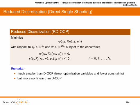
Reduced Discretization (RD-OCP)Minimize
ϕ(x0, XN (x0,w))
with respect to x0 ∈ Rnx and w ∈ RMnu subject to the constraints
ψ(x0, XN (x0,w)) = 0,
c(tj , Xj (x0,w), uh(tj ; w)) ≤ 0, j = 0, 1, . . . ,N.
Remarks:I much smaller than D-OCP (fewer optimization variables and fewer constraints)I but: more nonlinear than D-OCP
Numerical Optimal Control – Part 2: Discretization techniques, structure exploitation, calculation of gradients –Matthias Gerdts
Reduced Discretization (Direct Single Shooting)
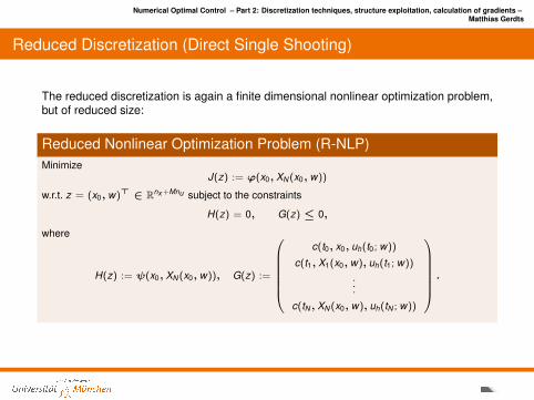
The reduced discretization is again a finite dimensional nonlinear optimization problem,but of reduced size:
Reduced Nonlinear Optimization Problem (R-NLP)Minimize
J(z) := ϕ(x0, XN (x0, w))
w.r.t. z = (x0, w)> ∈ Rnx +Mnu subject to the constraints
H(z) = 0, G(z) ≤ 0,
where
H(z) := ψ(x0, XN (x0, w)), G(z) :=
c(t0, x0, uh(t0; w))
c(t1, X1(x0, w), uh(t1; w))
...
c(tN , XN (x0, w), uh(tN ; w))
.
Numerical Optimal Control – Part 2: Discretization techniques, structure exploitation, calculation of gradients –Matthias Gerdts
Reduced Discretization (Direct Single Shooting)
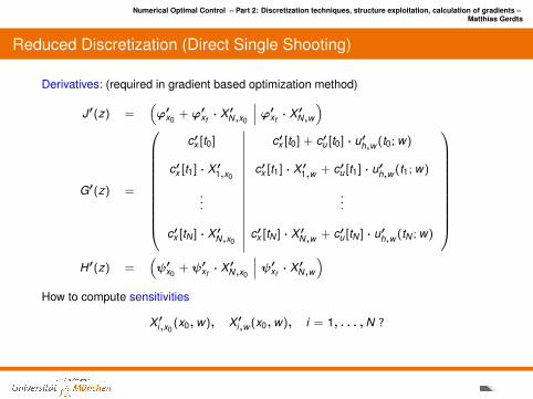
Derivatives: (required in gradient based optimization method)
J′(z) =(ϕ′x0
+ ϕ′xf· X ′N,x0
∣∣∣ ϕ′xf· X ′N,w
)
G′(z) =
c′x [t0] c′x [t0] + c′u [t0] · u′h,w (t0; w)
c′x [t1] · X ′1,x0c′x [t1] · X ′1,w + c′u [t1] · u′h,w (t1; w)
......
c′x [tN ] · X ′N,x0c′x [tN ] · X ′N,w + c′u [tN ] · u′h,w (tN ; w)
H′(z) =
(ψ′x0
+ ψ′xf· X ′N,x0
∣∣∣ ψ′xf· X ′N,w
)How to compute sensitivities
X ′i,x0(x0,w), X ′i,w (x0,w), i = 1, . . . ,N ?
Numerical Optimal Control – Part 2: Discretization techniques, structure exploitation, calculation of gradients –Matthias Gerdts
Computation of Derivatives
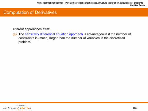
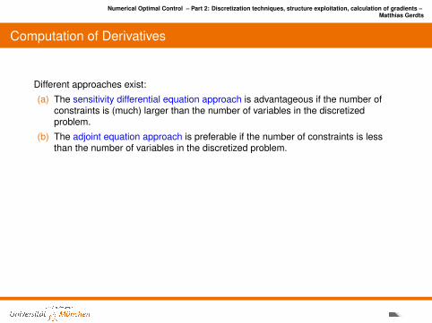
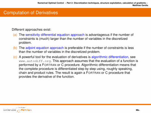
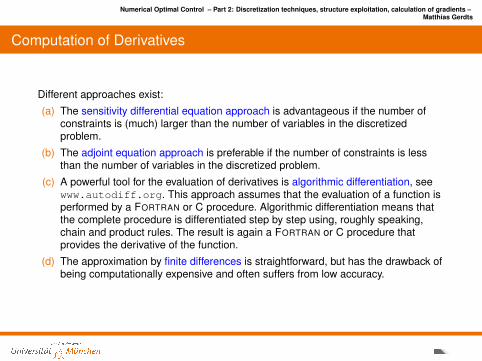
Different approaches exist:
(a) The sensitivity differential equation approach is advantageous if the number ofconstraints is (much) larger than the number of variables in the discretizedproblem.
(b) The adjoint equation approach is preferable if the number of constraints is lessthan the number of variables in the discretized problem.
(c) A powerful tool for the evaluation of derivatives is algorithmic differentiation, seewww.autodiff.org. This approach assumes that the evaluation of a function isperformed by a FORTRAN or C procedure. Algorithmic differentiation means thatthe complete procedure is differentiated step by step using, roughly speaking,chain and product rules. The result is again a FORTRAN or C procedure thatprovides the derivative of the function.
(d) The approximation by finite differences is straightforward, but has the drawback ofbeing computationally expensive and often suffers from low accuracy.
Numerical Optimal Control – Part 2: Discretization techniques, structure exploitation, calculation of gradients –Matthias Gerdts
Computation of Derivatives
Different approaches exist:
(a) The sensitivity differential equation approach is advantageous if the number ofconstraints is (much) larger than the number of variables in the discretizedproblem.
(b) The adjoint equation approach is preferable if the number of constraints is lessthan the number of variables in the discretized problem.
(c) A powerful tool for the evaluation of derivatives is algorithmic differentiation, seewww.autodiff.org. This approach assumes that the evaluation of a function isperformed by a FORTRAN or C procedure. Algorithmic differentiation means thatthe complete procedure is differentiated step by step using, roughly speaking,chain and product rules. The result is again a FORTRAN or C procedure thatprovides the derivative of the function.
(d) The approximation by finite differences is straightforward, but has the drawback ofbeing computationally expensive and often suffers from low accuracy.
Numerical Optimal Control – Part 2: Discretization techniques, structure exploitation, calculation of gradients –Matthias Gerdts
Computation of Derivatives by Sensitivity Analysis
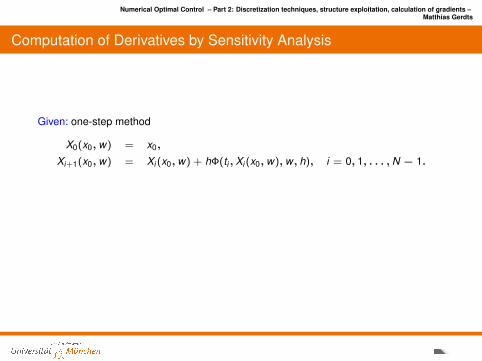
Given: one-step method
X0(x0,w) = x0,
Xi+1(x0,w) = Xi (x0,w) + hΦ(ti , Xi (x0,w),w, h), i = 0, 1, . . . ,N − 1.
Goal: Compute sensitivities
Si := X ′i (x0,w) =(
X ′i,x0(x0,w) X ′i,w (x0,w)
), i = 0, 1, . . . ,N.
Idea: Differentiate the one-step method step-by-step with respect to x0 and w .
Numerical Optimal Control – Part 2: Discretization techniques, structure exploitation, calculation of gradients –Matthias Gerdts
Computation of Derivatives by Sensitivity Analysis
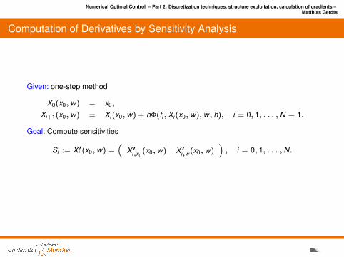
Given: one-step method
X0(x0,w) = x0,
Xi+1(x0,w) = Xi (x0,w) + hΦ(ti , Xi (x0,w),w, h), i = 0, 1, . . . ,N − 1.
Goal: Compute sensitivities
Si := X ′i (x0,w) =(
X ′i,x0(x0,w) X ′i,w (x0,w)
), i = 0, 1, . . . ,N.
Idea: Differentiate the one-step method step-by-step with respect to x0 and w .
Numerical Optimal Control – Part 2: Discretization techniques, structure exploitation, calculation of gradients –Matthias Gerdts
Computation of Derivatives by Sensitivity Analysis
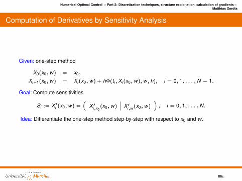
Given: one-step method
X0(x0,w) = x0,
Xi+1(x0,w) = Xi (x0,w) + hΦ(ti , Xi (x0,w),w, h), i = 0, 1, . . . ,N − 1.
Goal: Compute sensitivities
Si := X ′i (x0,w) =(
X ′i,x0(x0,w) X ′i,w (x0,w)
), i = 0, 1, . . . ,N.
Idea: Differentiate the one-step method step-by-step with respect to x0 and w .
Numerical Optimal Control – Part 2: Discretization techniques, structure exploitation, calculation of gradients –Matthias Gerdts
Computation of Derivatives by Sensitivity Analysis
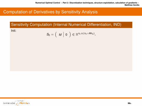
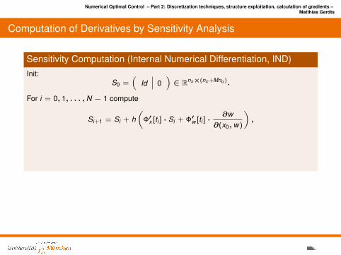
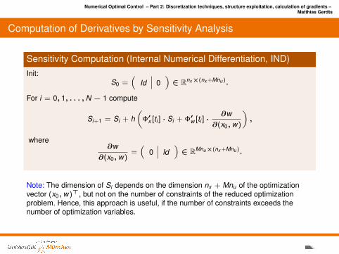
Sensitivity Computation (Internal Numerical Differentiation, IND)Init:
S0 =(
Id 0)∈ Rnx×(nx +Mnu).
For i = 0, 1, . . . ,N − 1 compute
Si+1 = Si + h(
Φ′x [ti ] · Si + Φ′w [ti ] ·∂w
∂(x0,w)
),
where∂w
∂(x0,w)=(
0 Id)∈ RMnu×(nx +Mnu).
Note: The dimension of Si depends on the dimension nx + Mnu of the optimizationvector (x0,w)>, but not on the number of constraints of the reduced optimizationproblem. Hence, this approach is useful, if the number of constraints exceeds thenumber of optimization variables.
Numerical Optimal Control – Part 2: Discretization techniques, structure exploitation, calculation of gradients –Matthias Gerdts
Computation of Derivatives by Sensitivity Analysis
Sensitivity Computation (Internal Numerical Differentiation, IND)Init:
S0 =(
Id 0)∈ Rnx×(nx +Mnu).
For i = 0, 1, . . . ,N − 1 compute
Si+1 = Si + h(
Φ′x [ti ] · Si + Φ′w [ti ] ·∂w
∂(x0,w)
),
where∂w
∂(x0,w)=(
0 Id)∈ RMnu×(nx +Mnu).
Note: The dimension of Si depends on the dimension nx + Mnu of the optimizationvector (x0,w)>, but not on the number of constraints of the reduced optimizationproblem. Hence, this approach is useful, if the number of constraints exceeds thenumber of optimization variables.
Numerical Optimal Control – Part 2: Discretization techniques, structure exploitation, calculation of gradients –Matthias Gerdts
Computation of Derivatives by Sensitivity Analysis
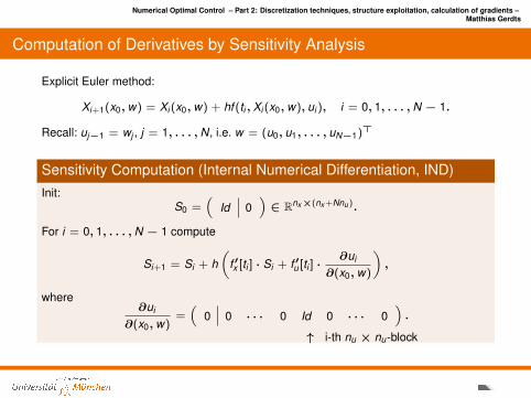
Explicit Euler method:
Xi+1(x0,w) = Xi (x0,w) + hf (ti , Xi (x0,w), ui ), i = 0, 1, . . . ,N − 1.
Recall: uj−1 = wj , j = 1, . . . ,N, i.e. w = (u0, u1, . . . , uN−1)>
Sensitivity Computation (Internal Numerical Differentiation, IND)Init:
S0 =(
Id 0)∈ Rnx×(nx +Nnu).
For i = 0, 1, . . . ,N − 1 compute
Si+1 = Si + h(
f ′x [ti ] · Si + f ′u [ti ] ·∂ui
∂(x0,w)
),
where∂ui
∂(x0,w)=(
0 0 · · · 0 Id 0 · · · 0).
↑ i-th nu × nu-block
Numerical Optimal Control – Part 2: Discretization techniques, structure exploitation, calculation of gradients –Matthias Gerdts
IND and Sensitivity Differential Equation
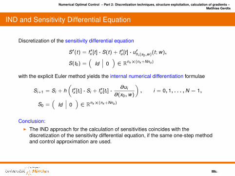
Discretization of the sensitivity differential equation
S′(t) = f ′x [t] · S(t) + f ′u [t] · u′h,(x0,w)(t ; w),
S(t0) =(
Id 0)∈ Rnx×(nx +Nnu)
with the explicit Euler method yields the internal numerical differentiation formulae
Si+1 = Si + h(
f ′x [ti ] · Si + f ′u [ti ] ·∂ui
∂(x0,w)
), i = 0, 1, . . . ,N − 1,
S0 =(
Id 0)∈ Rnx×(nx +Nnu)
Conclusion:I The IND approach for the calculation of sensitivities coincides with the
discretization of the sensitivity differential equation, if the same one-step methodand control approximation are used.
Numerical Optimal Control – Part 2: Discretization techniques, structure exploitation, calculation of gradients –Matthias Gerdts
Gradient Computation by Adjoint Equation
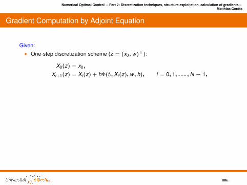
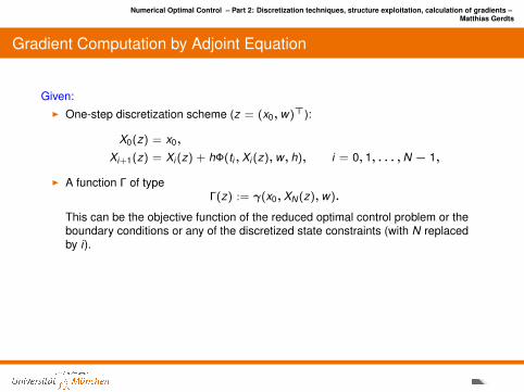
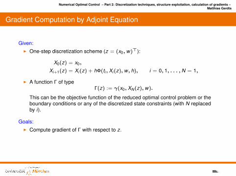
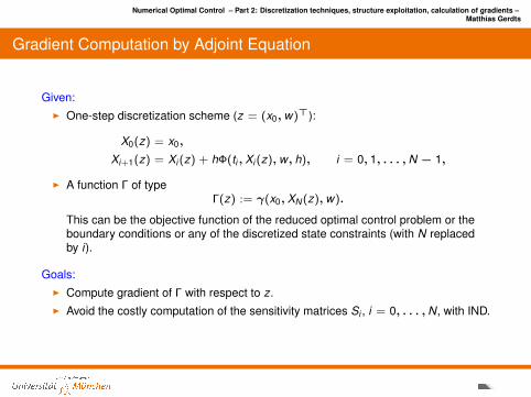
Given:I One-step discretization scheme (z = (x0,w)>):
X0(z) = x0,
Xi+1(z) = Xi (z) + hΦ(ti , Xi (z),w, h), i = 0, 1, . . . ,N − 1,
I A function Γ of typeΓ(z) := γ(x0, XN (z),w).
This can be the objective function of the reduced optimal control problem or theboundary conditions or any of the discretized state constraints (with N replacedby i).
Goals:
I Compute gradient of Γ with respect to z.I Avoid the costly computation of the sensitivity matrices Si , i = 0, . . . ,N, with IND.
Numerical Optimal Control – Part 2: Discretization techniques, structure exploitation, calculation of gradients –Matthias Gerdts
Gradient Computation by Adjoint Equation
Given:I One-step discretization scheme (z = (x0,w)>):
X0(z) = x0,
Xi+1(z) = Xi (z) + hΦ(ti , Xi (z),w, h), i = 0, 1, . . . ,N − 1,
I A function Γ of typeΓ(z) := γ(x0, XN (z),w).
This can be the objective function of the reduced optimal control problem or theboundary conditions or any of the discretized state constraints (with N replacedby i).
Goals:I Compute gradient of Γ with respect to z.
I Avoid the costly computation of the sensitivity matrices Si , i = 0, . . . ,N, with IND.
Numerical Optimal Control – Part 2: Discretization techniques, structure exploitation, calculation of gradients –Matthias Gerdts
Gradient Computation by Adjoint Equation
Given:I One-step discretization scheme (z = (x0,w)>):
X0(z) = x0,
Xi+1(z) = Xi (z) + hΦ(ti , Xi (z),w, h), i = 0, 1, . . . ,N − 1,
I A function Γ of typeΓ(z) := γ(x0, XN (z),w).
This can be the objective function of the reduced optimal control problem or theboundary conditions or any of the discretized state constraints (with N replacedby i).
Goals:I Compute gradient of Γ with respect to z.I Avoid the costly computation of the sensitivity matrices Si , i = 0, . . . ,N, with IND.
Numerical Optimal Control – Part 2: Discretization techniques, structure exploitation, calculation of gradients –Matthias Gerdts
Gradient Computation by Adjoint Equation
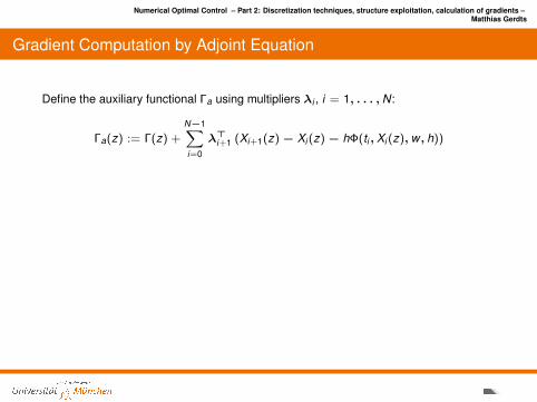
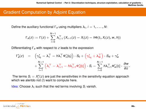
Define the auxiliary functional Γa using multipliers λi , i = 1, . . . ,N:
Γa(z) := Γ(z) +
N−1∑i=0
λ>i+1 (Xi+1(z)− Xi (z)− hΦ(ti , Xi (z),w, h))
Differentiating Γa with respect to z leads to the expression
Γ′a(z) =(γ′x0− λ>1 − hλ>1 Φ′x [t0]
)· S0 +
(γ′xN
+ λ>N
)· SN + γ′w
+
N−1∑i=1
(λ>i − λ
>i+1 − hλ>i+1Φ′x [ti ]
)· Si −
N−1∑i=0
hλ>i+1Φ′w [ti ] ·∂w∂z.
The terms Si = X ′i (z) are just the sensitivities in the sensitivity equation approachwhich we alertdo not (!) want to compute here.
Idea: Choose λi such that the red terms involving Si vanish.
Numerical Optimal Control – Part 2: Discretization techniques, structure exploitation, calculation of gradients –Matthias Gerdts
Gradient Computation by Adjoint Equation
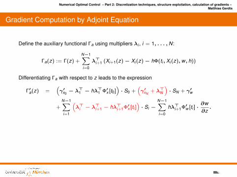
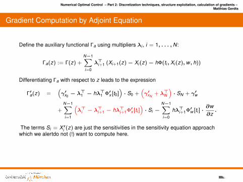
Define the auxiliary functional Γa using multipliers λi , i = 1, . . . ,N:
Γa(z) := Γ(z) +
N−1∑i=0
λ>i+1 (Xi+1(z)− Xi (z)− hΦ(ti , Xi (z),w, h))
Differentiating Γa with respect to z leads to the expression
Γ′a(z) =(γ′x0− λ>1 − hλ>1 Φ′x [t0]
)· S0 +
(γ′xN
+ λ>N
)· SN + γ′w
+
N−1∑i=1
(λ>i − λ
>i+1 − hλ>i+1Φ′x [ti ]
)· Si −
N−1∑i=0
hλ>i+1Φ′w [ti ] ·∂w∂z.
The terms Si = X ′i (z) are just the sensitivities in the sensitivity equation approachwhich we alertdo not (!) want to compute here.
Idea: Choose λi such that the red terms involving Si vanish.
Numerical Optimal Control – Part 2: Discretization techniques, structure exploitation, calculation of gradients –Matthias Gerdts
Gradient Computation by Adjoint Equation
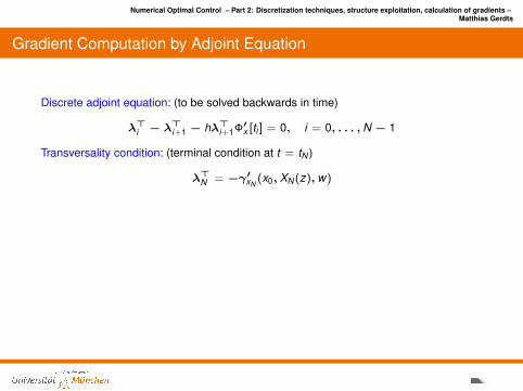
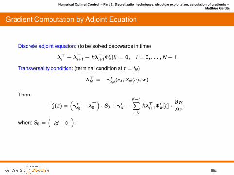
Discrete adjoint equation: (to be solved backwards in time)
λ>i − λ>i+1 − hλ>i+1Φ′x [ti ] = 0, i = 0, . . . ,N − 1
Transversality condition: (terminal condition at t = tN )
λ>N = −γ′xN(x0, XN (z),w)
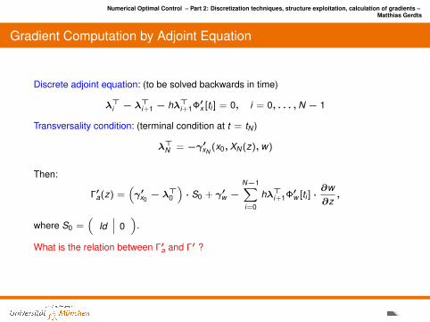
Then:
Γ′a(z) =(γ′x0− λ>0
)· S0 + γ′w −
N−1∑i=0
hλ>i+1Φ′w [ti ] ·∂w∂z,
where S0 =(
Id 0)
.
What is the relation between Γ′a and Γ′ ?
Numerical Optimal Control – Part 2: Discretization techniques, structure exploitation, calculation of gradients –Matthias Gerdts
Gradient Computation by Adjoint Equation
Discrete adjoint equation: (to be solved backwards in time)
λ>i − λ>i+1 − hλ>i+1Φ′x [ti ] = 0, i = 0, . . . ,N − 1
Transversality condition: (terminal condition at t = tN )
λ>N = −γ′xN(x0, XN (z),w)
Then:
Γ′a(z) =(γ′x0− λ>0
)· S0 + γ′w −
N−1∑i=0
hλ>i+1Φ′w [ti ] ·∂w∂z,
where S0 =(
Id 0)
.
What is the relation between Γ′a and Γ′ ?
Numerical Optimal Control – Part 2: Discretization techniques, structure exploitation, calculation of gradients –Matthias Gerdts
Gradient Computation by Adjoint Equation
TheoremIt holds
Γ′(z) = Γ′a(z) =(γ′x0− λ>0
)· S0 + γ′w −
N−1∑i=0
hλ>i+1Φ′w [ti ] ·∂w∂z.
Notes:
I With Γ′(z) = Γ′a(z) we found a formula for the gradient of Γ.I The size of the adjoint equation does not depend on the dimension of w and in
particular not on the number N that defines the grid. But an individual adjointequation has to be solved for every function whose gradient is required. For thereduced optimal control problem these functions are the objective function, theboundary conditions, and the discretized state constraints.
Numerical Optimal Control – Part 2: Discretization techniques, structure exploitation, calculation of gradients –Matthias Gerdts
Gradient Computation by Adjoint Equation
TheoremIt holds
Γ′(z) = Γ′a(z) =(γ′x0− λ>0
)· S0 + γ′w −
N−1∑i=0
hλ>i+1Φ′w [ti ] ·∂w∂z.
Notes:I With Γ′(z) = Γ′a(z) we found a formula for the gradient of Γ.
I The size of the adjoint equation does not depend on the dimension of w and inparticular not on the number N that defines the grid. But an individual adjointequation has to be solved for every function whose gradient is required. For thereduced optimal control problem these functions are the objective function, theboundary conditions, and the discretized state constraints.
Numerical Optimal Control – Part 2: Discretization techniques, structure exploitation, calculation of gradients –Matthias Gerdts
Gradient Computation by Adjoint Equation
TheoremIt holds
Γ′(z) = Γ′a(z) =(γ′x0− λ>0
)· S0 + γ′w −
N−1∑i=0
hλ>i+1Φ′w [ti ] ·∂w∂z.
Notes:I With Γ′(z) = Γ′a(z) we found a formula for the gradient of Γ.I The size of the adjoint equation does not depend on the dimension of w and in
particular not on the number N that defines the grid. But an individual adjointequation has to be solved for every function whose gradient is required. For thereduced optimal control problem these functions are the objective function, theboundary conditions, and the discretized state constraints.
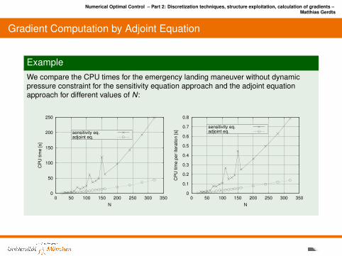
Numerical Optimal Control – Part 2: Discretization techniques, structure exploitation, calculation of gradients –Matthias Gerdts
Gradient Computation by Adjoint Equation
ExampleWe compare the CPU times for the emergency landing maneuver without dynamicpressure constraint for the sensitivity equation approach and the adjoint equationapproach for different values of N:
0
50
100
150
200
250
0 50 100 150 200 250 300 350
CP
U tim
e [s]
N
sensitivity eq. adjoint eq.
0
0.1
0.2
0.3
0.4
0.5
0.6
0.7
0.8
0 50 100 150 200 250 300 350
CP
U tim
e p
er
itera
tion [s]
N
sensitivity eq. adjoint eq.
Numerical Optimal Control – Part 2: Discretization techniques, structure exploitation, calculation of gradients –Matthias Gerdts
Contents
Direct Discretization MethodsFull DiscretizationReduced Discretization and Shooting MethodsAdjoint EstimationConvergenceExamples
Mixed-Integer Optimal ControlVariable Time Transformation
Parametric Sensitivity Analysis and Realtime-OptimizationParametric Optimal Control Problems
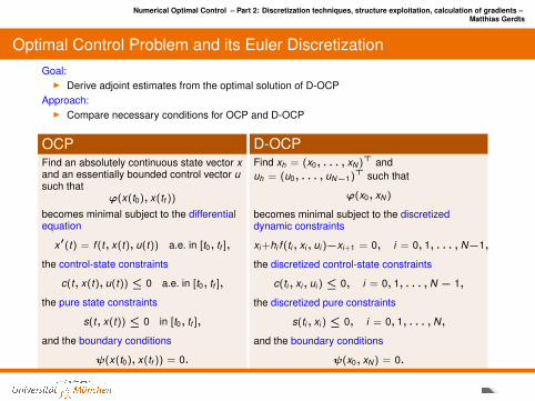
Numerical Optimal Control – Part 2: Discretization techniques, structure exploitation, calculation of gradients –Matthias Gerdts
Optimal Control Problem and its Euler DiscretizationGoal:
I Derive adjoint estimates from the optimal solution of D-OCPApproach:
I Compare necessary conditions for OCP and D-OCP
OCPFind an absolutely continuous state vector xand an essentially bounded control vector usuch that
ϕ(x(t0), x(tf ))
becomes minimal subject to the differentialequation
x′(t) = f (t, x(t), u(t)) a.e. in [t0, tf ],
the control-state constraints
c(t, x(t), u(t)) ≤ 0 a.e. in [t0, tf ],
the pure state constraints
s(t, x(t)) ≤ 0 in [t0, tf ],
and the boundary conditions
ψ(x(t0), x(tf )) = 0.
D-OCPFind xh = (x0, . . . , xN )> anduh = (u0, . . . , uN−1)> such that
ϕ(x0, xN )
becomes minimal subject to the discretizeddynamic constraints
xi +hi f (ti , xi , ui )−xi+1 = 0, i = 0, 1, . . . , N−1,
the discretized control-state constraints
c(ti , xi , ui ) ≤ 0, i = 0, 1, . . . , N − 1,
the discretized pure constraints
s(ti , xi ) ≤ 0, i = 0, 1, . . . , N,
and the boundary conditions
ψ(x0, xN ) = 0.
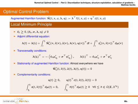
Numerical Optimal Control – Part 2: Discretization techniques, structure exploitation, calculation of gradients –Matthias Gerdts
Optimal Control ProblemAugmented Hamilton function: H(t, x, u, λ, η) := λ
>f (t, x, u) + η>c(t, x, u)
Local Minimum Principle
I `0 ≥ 0, (`0, σ, λ, η) 6= 0I Adjoint differential equation:
λ(t) = λ(tf ) +
∫ tf
tH′x (τ, x(τ ), u(τ ), λ(τ ), η(τ ))>dt +
∫ tf
ts′x (τ, x(τ ))>dµ(τ )
I Transversality conditions:
λ(t0)> = −(`0ϕ′x0
+ σ>ψ′x0
), λ(tf )> = `0ϕ
′xf
+ σ>ψ′xf
I Stationarity of augmented Hamilton function: Almost everywhere we have
H′u(t, x(t), u(t), λ(t), η(t)) = 0
I Complementarity conditions:
η(t) ≥ 0, η(t)>c(t, x(t), u(t)) = 0∫ tf
t0
s(t, x(t))>dµ(t) = 0,∫ tf
t0
h(t)>dµ(t) ≥ 0 ∀0 ≤ h ∈ C(I, Rns )
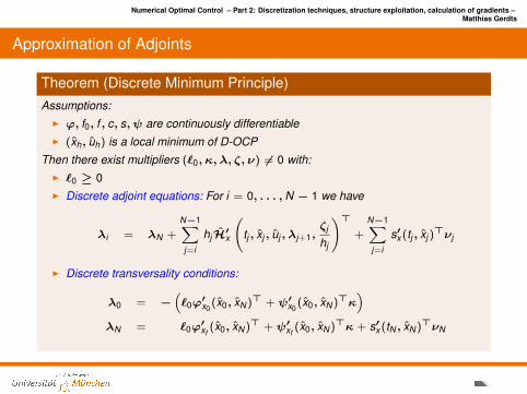
Numerical Optimal Control – Part 2: Discretization techniques, structure exploitation, calculation of gradients –Matthias Gerdts
Approximation of Adjoints
Theorem (Discrete Minimum Principle)Assumptions:
I ϕ, f0, f , c, s, ψ are continuously differentiableI (xh, uh) is a local minimum of D-OCP
Then there exist multipliers (`0, κ, λ, ζ, ν) 6= 0 with:I `0 ≥ 0I Discrete adjoint equations: For i = 0, . . . ,N − 1 we have
λi = λN +
N−1∑j=i
hjH′x
(tj , xj , uj , λj+1,
ζj
hj
)>+
N−1∑j=i
s′x (tj , xj )>νj
I Discrete transversality conditions:
λ0 = −(`0ϕ′x0
(x0, xN )> + ψ′x0(x0, xN )>κ
)λN = `0ϕ
′xf
(x0, xN )> + ψ′xf(x0, xN )>κ + s′x (tN , xN )>νN
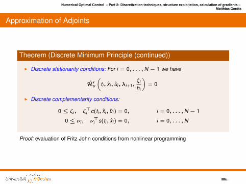
Numerical Optimal Control – Part 2: Discretization techniques, structure exploitation, calculation of gradients –Matthias Gerdts
Approximation of Adjoints
Theorem (Discrete Minimum Principle (continued))
I Discrete stationarity conditions: For i = 0, . . . ,N − 1 we have
H′u(
ti , xi , ui , λi+1,ζi
hi
)= 0
I Discrete complementarity conditions:
0 ≤ ζi , ζ>i c(ti , xi , ui ) = 0, i = 0, . . . ,N − 1
0 ≤ νi , ν>i s(ti , xi ) = 0, i = 0, . . . ,N
Proof: evaluation of Fritz John conditions from nonlinear programming
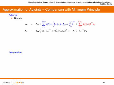
Numerical Optimal Control – Part 2: Discretization techniques, structure exploitation, calculation of gradients –Matthias Gerdts
Approximation of Adjoints – Comparison with Minimum PrincipleAdjoints:
I Discrete:
λi = λN +
N−1∑j=i
hjH′x(
tj , xj , uj , λj+1,ζj
hj
)>+
N−1∑j=i
s′x (tj , xj )>νj
λN = `0ϕ′xf
(x0, xN )> + ψ′xf(x0, xN )>κ + s′x (tN , xN )>νN
I Continuous:
λ(t) = λ(tf ) +
∫ tf
tH′x (t, x(t), u(t), λ(t), η(t))>dt +
∫ tf
ts′x (t, x(t))>dµ(t)
λ(tf ) = `0ϕ′xf
(x(t0), x(tf ))> + ψ′xf(x(t0), x(tf ))>σ
Interpretation:
I κ ≈ σ, λi ≈ λ(ti ), ζihi≈ η(ti )
I νi ≈ µ(ti+1)− µ(ti ), i = 0, . . . , N − 1I νN is interpreted as jump height at t = tf , i.e.
νN ≈ µ(tf )− µ(t−f ).
Note that µ can jump at tf .
I λN is interpreted as the left-sided limit of λ at tf , i.e. λN ≈ λ(t−f ). Note that λ may jump at tf .
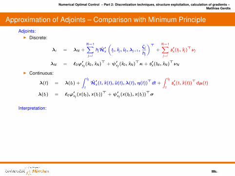
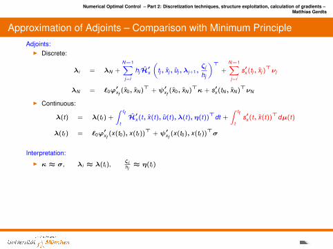
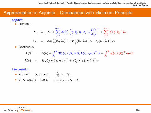
Numerical Optimal Control – Part 2: Discretization techniques, structure exploitation, calculation of gradients –Matthias Gerdts
Approximation of Adjoints – Comparison with Minimum PrincipleAdjoints:
I Discrete:
λi = λN +
N−1∑j=i
hjH′x(
tj , xj , uj , λj+1,ζj
hj
)>+
N−1∑j=i
s′x (tj , xj )>νj
λN = `0ϕ′xf
(x0, xN )> + ψ′xf(x0, xN )>κ + s′x (tN , xN )>νN
I Continuous:
λ(t) = λ(tf ) +
∫ tf
tH′x (t, x(t), u(t), λ(t), η(t))>dt +
∫ tf
ts′x (t, x(t))>dµ(t)
λ(tf ) = `0ϕ′xf
(x(t0), x(tf ))> + ψ′xf(x(t0), x(tf ))>σ
Interpretation:
I κ ≈ σ, λi ≈ λ(ti ), ζihi≈ η(ti )
I νi ≈ µ(ti+1)− µ(ti ), i = 0, . . . , N − 1
I νN is interpreted as jump height at t = tf , i.e.
νN ≈ µ(tf )− µ(t−f ).
Note that µ can jump at tf .
I λN is interpreted as the left-sided limit of λ at tf , i.e. λN ≈ λ(t−f ). Note that λ may jump at tf .
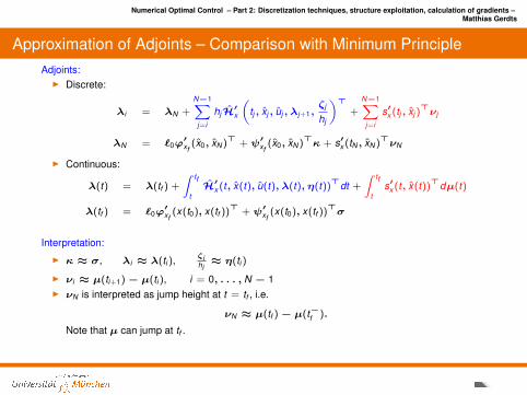
Numerical Optimal Control – Part 2: Discretization techniques, structure exploitation, calculation of gradients –Matthias Gerdts
Approximation of Adjoints – Comparison with Minimum PrincipleAdjoints:
I Discrete:
λi = λN +
N−1∑j=i
hjH′x(
tj , xj , uj , λj+1,ζj
hj
)>+
N−1∑j=i
s′x (tj , xj )>νj
λN = `0ϕ′xf
(x0, xN )> + ψ′xf(x0, xN )>κ + s′x (tN , xN )>νN
I Continuous:
λ(t) = λ(tf ) +
∫ tf
tH′x (t, x(t), u(t), λ(t), η(t))>dt +
∫ tf
ts′x (t, x(t))>dµ(t)
λ(tf ) = `0ϕ′xf
(x(t0), x(tf ))> + ψ′xf(x(t0), x(tf ))>σ
Interpretation:
I κ ≈ σ, λi ≈ λ(ti ), ζihi≈ η(ti )
I νi ≈ µ(ti+1)− µ(ti ), i = 0, . . . , N − 1I νN is interpreted as jump height at t = tf , i.e.
νN ≈ µ(tf )− µ(t−f ).
Note that µ can jump at tf .
I λN is interpreted as the left-sided limit of λ at tf , i.e. λN ≈ λ(t−f ). Note that λ may jump at tf .
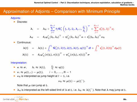
Numerical Optimal Control – Part 2: Discretization techniques, structure exploitation, calculation of gradients –Matthias Gerdts
Approximation of Adjoints – Comparison with Minimum PrincipleAdjoints:
I Discrete:
λi = λN +
N−1∑j=i
hjH′x(
tj , xj , uj , λj+1,ζj
hj
)>+
N−1∑j=i
s′x (tj , xj )>νj
λN = `0ϕ′xf
(x0, xN )> + ψ′xf(x0, xN )>κ + s′x (tN , xN )>νN
I Continuous:
λ(t) = λ(tf ) +
∫ tf
tH′x (t, x(t), u(t), λ(t), η(t))>dt +
∫ tf
ts′x (t, x(t))>dµ(t)
λ(tf ) = `0ϕ′xf
(x(t0), x(tf ))> + ψ′xf(x(t0), x(tf ))>σ
Interpretation:
I κ ≈ σ, λi ≈ λ(ti ), ζihi≈ η(ti )
I νi ≈ µ(ti+1)− µ(ti ), i = 0, . . . , N − 1I νN is interpreted as jump height at t = tf , i.e.
νN ≈ µ(tf )− µ(t−f ).
Note that µ can jump at tf .
I λN is interpreted as the left-sided limit of λ at tf , i.e. λN ≈ λ(t−f ). Note that λ may jump at tf .
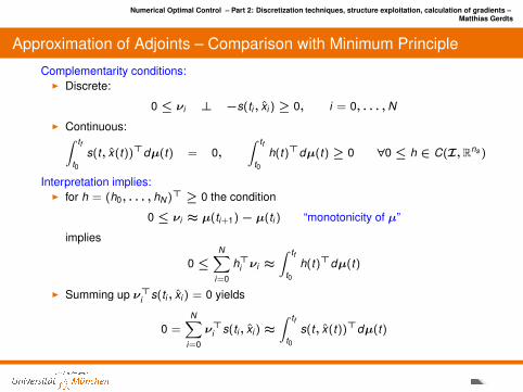
Numerical Optimal Control – Part 2: Discretization techniques, structure exploitation, calculation of gradients –Matthias Gerdts
Approximation of Adjoints – Comparison with Minimum Principle
Complementarity conditions:I Discrete:
0 ≤ νi ⊥ −s(ti , xi ) ≥ 0, i = 0, . . . ,N
I Continuous:∫ tf
t0s(t, x(t))>dµ(t) = 0,
∫ tf
t0h(t)>dµ(t) ≥ 0 ∀0 ≤ h ∈ C(I,Rns )
Interpretation implies:I for h = (h0, . . . , hN )> ≥ 0 the condition
0 ≤ νi ≈ µ(ti+1)− µ(ti ) “monotonicity of µ”
implies
0 ≤N∑
i=0
h>i νi ≈∫ tf
t0h(t)>dµ(t)
I Summing up ν>i s(ti , xi ) = 0 yields
0 =N∑
i=0
ν>i s(ti , xi ) ≈∫ tf
t0s(t, x(t))>dµ(t)
Numerical Optimal Control – Part 2: Discretization techniques, structure exploitation, calculation of gradients –Matthias Gerdts
Contents
Direct Discretization MethodsFull DiscretizationReduced Discretization and Shooting MethodsAdjoint EstimationConvergenceExamples
Mixed-Integer Optimal ControlVariable Time Transformation
Parametric Sensitivity Analysis and Realtime-OptimizationParametric Optimal Control Problems
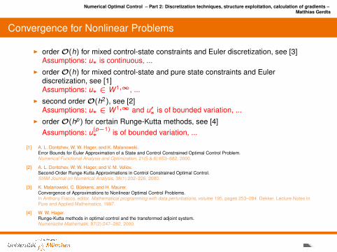
Numerical Optimal Control – Part 2: Discretization techniques, structure exploitation, calculation of gradients –Matthias Gerdts
Convergence for Nonlinear Problems
I orderO(h) for mixed control-state constraints and Euler discretization, see [3]Assumptions: u∗ is continuous, ...
I orderO(h) for mixed control-state and pure state constraints and Eulerdiscretization, see [1]Assumptions: u∗ ∈ W 1,∞, ...
I second orderO(h2), see [2]Assumptions: u∗ ∈ W 1,∞ and u′∗ is of bounded variation, ...
I orderO(hp) for certain Runge-Kutta methods, see [4]Assumptions: u(p−1)
∗ is of bounded variation, ...
[1] A. L. Dontchev, W. W. Hager, and K. Malanowski.Error Bounds for Euler Approximation of a State and Control Constrained Optimal Control Problem.Numerical Functional Analysis and Optimization, 21(5 & 6):653–682, 2000.
[2] A. L. Dontchev, W. W. Hager, and V. M. Veliov.Second-Order Runge-Kutta Approximations in Control Constrained Optimal Control.SIAM Journal on Numerical Analysis, 38(1):202–226, 2000.
[3] K. Malanowski, C. Buskens, and H. Maurer.Convergence of Approximations to Nonlinear Optimal Control Problems.In Anthony Fiacco, editor, Mathematical programming with data perturbations, volume 195, pages 253–284. Dekker. Lecture Notes inPure and Applied Mathematics, 1997.
[4] W. W. Hager.Runge-Kutta methods in optimal control and the transformed adjoint system.Numerische Mathematik, 87(2):247–282, 2000.
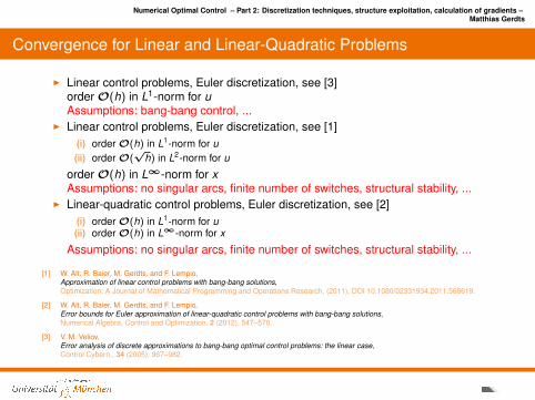
Numerical Optimal Control – Part 2: Discretization techniques, structure exploitation, calculation of gradients –Matthias Gerdts
Convergence for Linear and Linear-Quadratic Problems
I Linear control problems, Euler discretization, see [3]orderO(h) in L1-norm for uAssumptions: bang-bang control, ...
I Linear control problems, Euler discretization, see [1](i) orderO(h) in L1-norm for u(ii) orderO(
√h) in L2-norm for u
orderO(h) in L∞-norm for xAssumptions: no singular arcs, finite number of switches, structural stability, ...
I Linear-quadratic control problems, Euler discretization, see [2](i) orderO(h) in L1-norm for u(ii) orderO(h) in L∞-norm for x
Assumptions: no singular arcs, finite number of switches, structural stability, ...
[1] W. Alt, R. Baier, M. Gerdts, and F. Lempio,Approximation of linear control problems with bang-bang solutions,Optimization: A Journal of Mathematical Programming and Operations Research, (2011), DOI 10.1080/02331934.2011.568619.
[2] W. Alt, R. Baier, M. Gerdts, and F. Lempio,Error bounds for Euler approximation of linear-quadratic control problems with bang-bang solutions,Numerical Algebra, Control and Optimization, 2 (2012), 547–570.
[3] V. M. Veliov,Error analysis of discrete approximations to bang-bang optimal control problems: the linear case,Control Cybern., 34 (2005), 967–982.
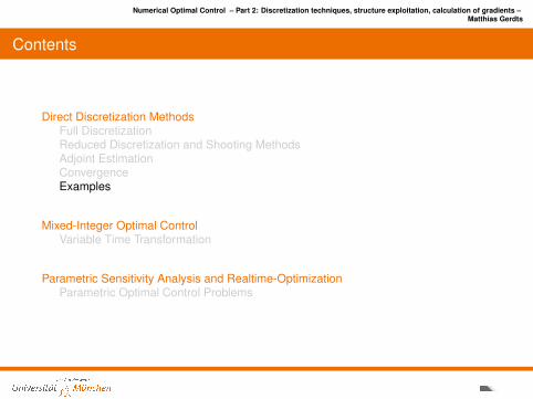
Numerical Optimal Control – Part 2: Discretization techniques, structure exploitation, calculation of gradients –Matthias Gerdts
Contents
Direct Discretization MethodsFull DiscretizationReduced Discretization and Shooting MethodsAdjoint EstimationConvergenceExamples
Mixed-Integer Optimal ControlVariable Time Transformation
Parametric Sensitivity Analysis and Realtime-OptimizationParametric Optimal Control Problems
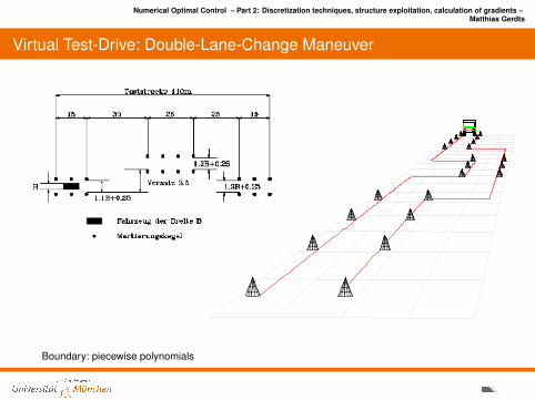
Numerical Optimal Control – Part 2: Discretization techniques, structure exploitation, calculation of gradients –Matthias Gerdts
Virtual Test-Drive: Double-Lane-Change Maneuver
Boundary: piecewise polynomials
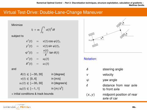
Numerical Optimal Control – Part 2: Discretization techniques, structure exploitation, calculation of gradients –Matthias Gerdts
Virtual Test-Drive: Double-Lane-Change Maneuver
Minimize
tf + α
∫ tf
0u(t)2dt
subject to
x′(t) = v(t) cosψ(t),
y′(t) = v(t) sinψ(t),
ψ′(t) =
v(t)`
tan δ(t)
v′(t) = u2(t)
δ′(t) = u1(t)
and
δ(t) ∈ [−30, 30] in [degree]
v(t) ∈ [0, 6] in [m/s]
u1(t) ∈ [−30, 30] in [degree/s]
u2(t) ∈ [−1, 1] in [m/s2]
+ initial conditions & track bounds
δ
δ
ψ(x,y)
l
Notation:
δ steering angle
v velocity
ψ yaw angle
` distance from rear axleto front axle
(x, y) midpoint position of rearaxle of car
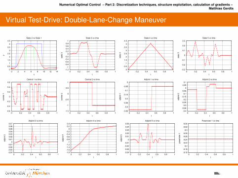
Numerical Optimal Control – Part 2: Discretization techniques, structure exploitation, calculation of gradients –Matthias Gerdts
Virtual Test-Drive: Double-Lane-Change Maneuver
0
0.5
1
1.5
2
2.5
3
3.5
4
4.5
0 2 4 6 8 10 12 14
y
x
State 2 vs State 1
-1.2
-1
-0.8
-0.6
-0.4
-0.2
0
0.2
0.4
0.6
0.8
1
0 0.2 0.4 0.6 0.8 1
sta
te 3
t
State 3 vs time
0
0.5
1
1.5
2
2.5
3
3.5
4
4.5
0 0.2 0.4 0.6 0.8 1
sta
te 4
t
State 4 vs time
-0.3
-0.2
-0.1
0
0.1
0.2
0.3
0 0.2 0.4 0.6 0.8 1
sta
te 5
t
State 5 vs time
-0.6
-0.4
-0.2
0
0.2
0.4
0.6
0 0.2 0.4 0.6 0.8 1
co
ntr
ol 1
t
Control 1 vs time
-1.5
-1
-0.5
0
0.5
1
0 0.2 0.4 0.6 0.8 1
co
ntr
ol 2
t
Control 2 vs time
-0.35
-0.3
-0.25
-0.2
-0.15
-0.1
-0.05
0
0 0.2 0.4 0.6 0.8 1
ad
join
t 1
t
Adjoint 1 vs time
-0.4
-0.35
-0.3
-0.25
-0.2
-0.15
-0.1
-0.05
0
0.05
0.1
0 0.2 0.4 0.6 0.8 1
ad
join
t 2
t
Adjoint 2 vs time
-0.04
-0.03
-0.02
-0.01
0
0.01
0.02
0.03
0.04
0.05
0.06
0.07
0 0.2 0.4 0.6 0.8 1
ad
join
t 3
t
Adjoint 3 vs time
-1.8
-1.6
-1.4
-1.2
-1
-0.8
-0.6
-0.4
-0.2
0
0.2
0.4
0 0.2 0.4 0.6 0.8 1
ad
join
t 4
t
Adjoint 4 vs time
-0.04
-0.03
-0.02
-0.01
0
0.01
0.02
0.03
0.04
0.05
0 0.2 0.4 0.6 0.8 1
ad
join
t 5
t
Adjoint 5 vs time
8.16
8.18
8.2
8.22
8.24
8.26
8.28
8.3
8.32
8.34
0 0.2 0.4 0.6 0.8 1
pa
ram
ete
r 1
t
Parameter 1 vs time
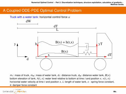
Numerical Optimal Control – Part 2: Discretization techniques, structure exploitation, calculation of gradients –Matthias Gerdts
A Coupled ODE-PDE Optimal Control Problem
Truck with a water tank: horizontal control force u
d
y
dT
yTh
B(x)
B(x) + h(t,x)
dW
LdT
x
mT : mass of truck, mW : mass of water tank, dT : distance truck, dW : distance water tank, B(x):bottom elevation of tank, h(t, x): water level relative to bottom at time t and position x , v(t, x):horizontal water velocity at time t and position x , L: length of water tank, c : spring force constant,k : damper force constant
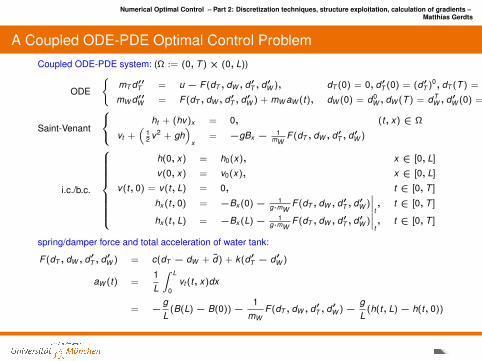
Numerical Optimal Control – Part 2: Discretization techniques, structure exploitation, calculation of gradients –Matthias Gerdts
A Coupled ODE-PDE Optimal Control ProblemCoupled ODE-PDE system: (Ω := (0, T )× (0, L))
ODE
mT d′′T = u − F (dT , dW , d′T , d′W ), dT (0) = 0, d′T (0) = (d′T )0, dT (T ) = dT
T ,
mW d′′W = F (dT , dW , d′T , d′W ) + mW aW (t), dW (0) = d0W , dW (T ) = dT
W , d′W (0) = (d′W )0
Saint-Venant
ht + (hv)x = 0, (t, x) ∈ Ω
vt +(
12 v2 + gh
)x
= −gBx − 1mW
F (dT , dW , d′T , d′W )
i.c./b.c.
h(0, x) = h0(x), x ∈ [0, L]
v(0, x) = v0(x), x ∈ [0, L]
v(t, 0) = v(t, L) = 0, t ∈ [0, T ]
hx (t, 0) = −Bx (0)− 1g·mW
F (dT , dW , d′T , d′W )∣∣∣
t, t ∈ [0, T ]
hx (t, L) = −Bx (L)− 1g·mW
F (dT , dW , d′T , d′W )∣∣∣
t, t ∈ [0, T ]
spring/damper force and total acceleration of water tank:
F (dT , dW , d′T , d′W ) = c(dT − dW + d) + k(d′T − d′W )
aW (t) =1L
∫ L
0vt (t, x)dx
= −gL
(B(L)− B(0))−1
mWF (dT , dW , d′T , d′W )−
gL
(h(t, L)− h(t, 0))
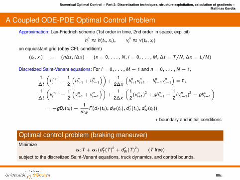
Numerical Optimal Control – Part 2: Discretization techniques, structure exploitation, calculation of gradients –Matthias Gerdts
A Coupled ODE-PDE Optimal Control ProblemApproximation: Lax-Friedrich scheme (1st order in time, 2nd order in space, explicit)
hni ≈ h(tn, xi ), vn
i ≈ v(tn, xi )
on equidistant grid (obey CFL condition!)
(tn, xi ) := (n∆t, i∆x) (n = 0, . . . , N, i = 0, . . . ,M,∆t = T/N,∆x = L/M)
Discretized Saint-Venant equations: For i = 0, . . . ,M − 1 and n = 0, . . . , N − 1,
1∆t
(hn+1
i −12
(hn
i+1 + hni−1
))+
12∆x
(hn
i+1vni+1 − hn
i−1vni−1
)= 0,
1∆t
(vn+1
i −12
(vn
i+1 + vni−1
))+
12∆x
(12
(vni+1)2 + ghn
i+1 −12
(vni−1)2 − ghn
i−1
)= −gBx (xi )−
1mW
F (dT (tn), dW (tn), d′T (tn), d′W (tn))
+ boundary and initial conditions
Optimal control problem (braking maneuver)Minimize
α0T + α1(d′T (T )2 + d′W (T )2) (T free)
subject to the discretized Saint-Venant equations, truck dynamics, and control bounds.
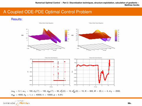
Numerical Optimal Control – Part 2: Discretization techniques, structure exploitation, calculation of gradients –Matthias Gerdts
A Coupled ODE-PDE Optimal Control Problem
Results:
0 2 4 6 8 10 12
0 0.5
1 1.5
2 2.5
3 3.5
4
0
0.5
1
1.5
2
2.5
h [m]
Trolley & Saint-Venant Equations
time [s]
x [m]
h [m]
0
0.5
1
1.5
2
2.5
0 2 4 6 8 10 12
0 0.5
1 1.5
2 2.5
3 3.5
4
-2.5-2
-1.5-1
-0.5 0
0.5 1
1.5 2
2.5
v [m]
Trolley & Saint-Venant Equations
time [s]
x [m]
v [m]
-2.5-2-1.5-1-0.5 0 0.5 1 1.5 2 2.5
-25000
-20000
-15000
-10000
-5000
0
5000
0 2 4 6 8 10 12
u [N
]
time [s]
Trolley & Saint-Venant Equations
-25000
-20000
-15000
-10000
-5000
0
5000
10000
0 2 4 6 8 10 12
F [N
]
time [s]
Trolley & Saint-Venant Equations
(α0 = 0.1,α1 = 100, dT (T ) = 100, dW (T ) = 95, d′T (0) = 10, d′W (0) = 10, N = 600, M = 20, L = 4, mT = 2000,
mW = 4000, h0 = 1, c = 40000, k = 10000, g = 9.81)
Numerical Optimal Control – Part 2: Discretization techniques, structure exploitation, calculation of gradients –Matthias Gerdts
Contents
Direct Discretization MethodsFull DiscretizationReduced Discretization and Shooting MethodsAdjoint EstimationConvergenceExamples
Mixed-Integer Optimal ControlVariable Time Transformation
Parametric Sensitivity Analysis and Realtime-OptimizationParametric Optimal Control Problems
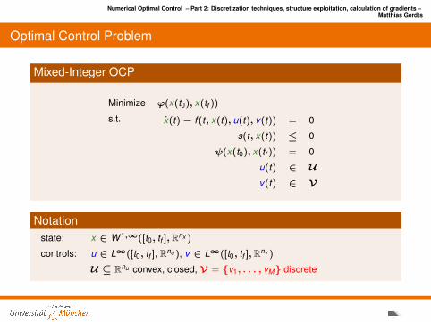
Numerical Optimal Control – Part 2: Discretization techniques, structure exploitation, calculation of gradients –Matthias Gerdts
Optimal Control Problem
Mixed-Integer OCP
Minimize ϕ(x(t0), x(tf ))
s.t. x(t)− f (t, x(t), u(t), v(t)) = 0
s(t, x(t)) ≤ 0
ψ(x(t0), x(tf )) = 0
u(t) ∈ Uv(t) ∈ V
Notationstate: x ∈ W 1,∞([t0, tf ],Rnx )
controls: u ∈ L∞([t0, tf ],Rnu ), v ∈ L∞([t0, tf ],Rnv )
U ⊆ Rnu convex, closed, V = v1, . . . , vM discrete
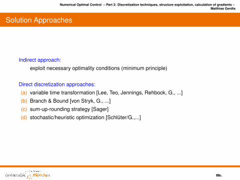
Numerical Optimal Control – Part 2: Discretization techniques, structure exploitation, calculation of gradients –Matthias Gerdts
Solution Approaches
Indirect approach:
exploit necessary optimality conditions (minimum principle)
Direct discretization approaches:
(a) variable time transformation [Lee, Teo, Jennings, Rehbock, G., ...]
(b) Branch & Bound [von Stryk, G., ...]
(c) sum-up-rounding strategy [Sager]
(d) stochastic/heuristic optimization [Schluter/G.,...]
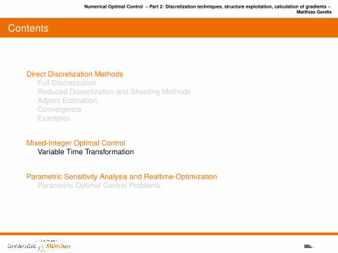
Numerical Optimal Control – Part 2: Discretization techniques, structure exploitation, calculation of gradients –Matthias Gerdts
Contents
Direct Discretization MethodsFull DiscretizationReduced Discretization and Shooting MethodsAdjoint EstimationConvergenceExamples
Mixed-Integer Optimal ControlVariable Time Transformation
Parametric Sensitivity Analysis and Realtime-OptimizationParametric Optimal Control Problems
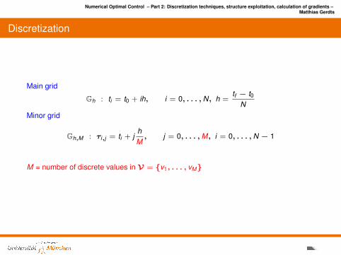
Numerical Optimal Control – Part 2: Discretization techniques, structure exploitation, calculation of gradients –Matthias Gerdts
Discretization
Main grid
Gh : ti = t0 + ih, i = 0, . . . ,N, h =tf − t0
NMinor grid
Gh,M : τi,j = ti + jhM, j = 0, . . . ,M, i = 0, . . . ,N − 1
M = number of discrete values in V = v1, . . . , vM
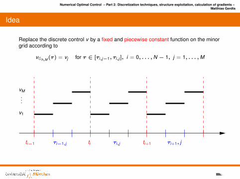
Numerical Optimal Control – Part 2: Discretization techniques, structure exploitation, calculation of gradients –Matthias Gerdts
Idea
Replace the discrete control v by a fixed and piecewise constant function on the minorgrid according to
vGh,M (τ ) = vj for τ ∈ [τi,j−1, τi,j ], i = 0, . . . ,N − 1, j = 1, . . . ,M
ti−1 ti ti+1τi−1,j τi,j τi+1, j
v1
...
vM
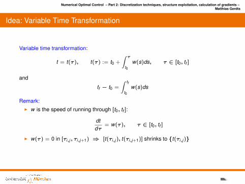
Numerical Optimal Control – Part 2: Discretization techniques, structure exploitation, calculation of gradients –Matthias Gerdts
Idea: Variable Time Transformation
Variable time transformation:
t = t(τ ), t(τ ) := t0 +
∫ τt0
w(s)ds, τ ∈ [t0, tf ]
and
tf − t0 =
∫ tf
t0w(s)ds
Remark:I w is the speed of running through [t0, tf ]:
dtdτ
= w(τ ), τ ∈ [t0, tf ]
I w(τ ) = 0 in [τi,j , τi,j+1) ⇒ [t(τi,j ), t(τi,j+1)] shrinks to t(τi,j )
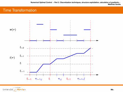
Numerical Optimal Control – Part 2: Discretization techniques, structure exploitation, calculation of gradients –Matthias Gerdts
Time Transformation
ti−1 ti ti+1τi−1,j τi,j τi+1, j
w(τ )
t(τ )
ti−1
ti
ti+1
ti+2
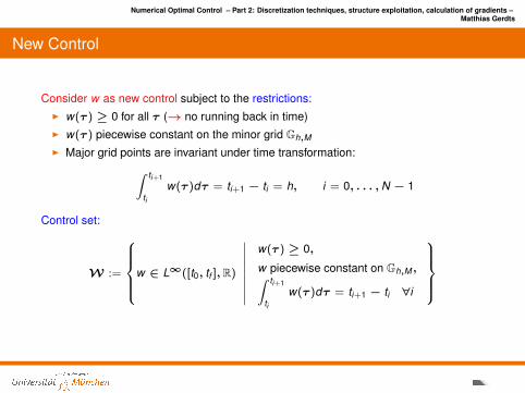
Numerical Optimal Control – Part 2: Discretization techniques, structure exploitation, calculation of gradients –Matthias Gerdts
New Control
Consider w as new control subject to the restrictions:I w(τ ) ≥ 0 for all τ (→ no running back in time)I w(τ ) piecewise constant on the minor grid Gh,M
I Major grid points are invariant under time transformation:∫ ti+1
tiw(τ )dτ = ti+1 − ti = h, i = 0, . . . ,N − 1
Control set:
W :=
w ∈ L∞([t0, tf ],R)
∣∣∣∣∣∣∣∣∣w(τ ) ≥ 0,
w piecewise constant on Gh,M ,∫ ti+1
tiw(τ )dτ = ti+1 − ti ∀i
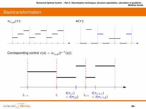
Numerical Optimal Control – Part 2: Discretization techniques, structure exploitation, calculation of gradients –Matthias Gerdts
Backtransformation
vGh,M (τ ): w(τ ):
Corresponding control v(s) = vGh,M (t−1(s)):
ti−1 ti ti+1t(τi,1)= t(τi,2)
t(τi+1,1)= t(τi+1,2)
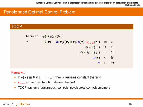
Numerical Optimal Control – Part 2: Discretization techniques, structure exploitation, calculation of gradients –Matthias Gerdts
Transformed Optimal Control Problem
TOCP
Minimize ϕ(x(t0), x(tf ))
s.t. x(τ )− w(τ )f (τ, x(τ ), u(τ ), vGh,M (τ )) = 0
s(τ, x(τ )) ≤ 0
ψ(x(t0), x(tf )) = 0
u(τ ) ∈ Uw ∈ W
Remarks:I If w(τ ) ≡ 0 in [τi,j , τi,j+1] then x remains constant therein!I vGh,M is the fixed function defined before!
I TOCP has only ‘continuous’ controls, no discrete controls anymore!
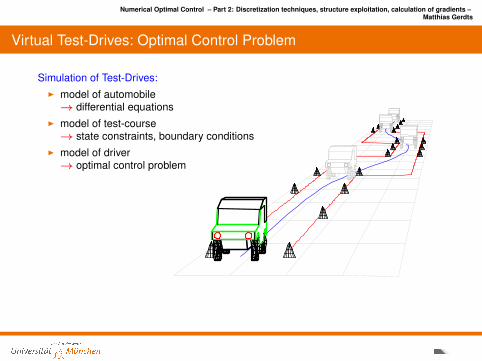
Numerical Optimal Control – Part 2: Discretization techniques, structure exploitation, calculation of gradients –Matthias Gerdts
Virtual Test-Drives: Optimal Control Problem
Simulation of Test-Drives:I model of automobile→ differential equations
I model of test-course→ state constraints, boundary conditions
I model of driver→ optimal control problem
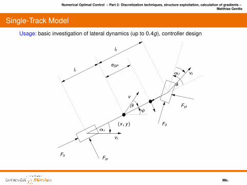
Numerical Optimal Control – Part 2: Discretization techniques, structure exploitation, calculation of gradients –Matthias Gerdts
Single-Track Model
Usage: basic investigation of lateral dynamics (up to 0.4g), controller design
lr
lf
eSP
FsrFlr
vr
αr
v
βψ
Flf
Fsf
αf vf
δ
(x, y)
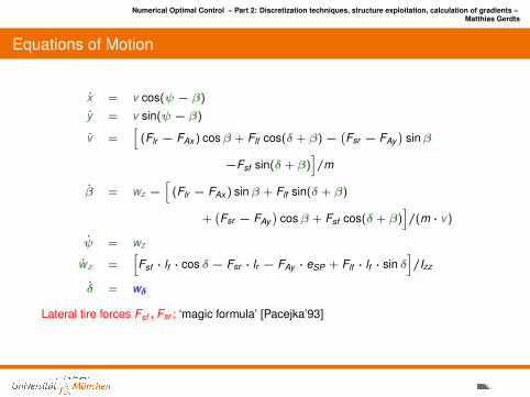
Numerical Optimal Control – Part 2: Discretization techniques, structure exploitation, calculation of gradients –Matthias Gerdts
Equations of Motion
x = v cos(ψ − β)
y = v sin(ψ − β)
v =[
(Flr − FAx ) cosβ + Flf cos(δ + β)−(Fsr − FAy
)sinβ
−Fsf sin(δ + β)]/m
β = wz −[
(Flr − FAx ) sinβ + Flf sin(δ + β)
+(Fsr − FAy
)cosβ + Fsf cos(δ + β)
]/(m · v)
ψ = wz
wz =[Fsf · lf · cos δ − Fsr · lr − FAy · eSP + Flf · lf · sin δ
]/Izz
δ = wδ
Lateral tire forces Fsf , Fsr : ‘magic formula’ [Pacejka’93]
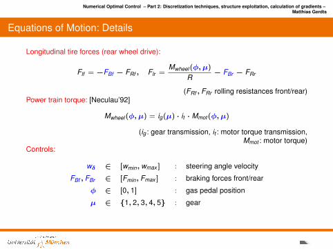
Numerical Optimal Control – Part 2: Discretization techniques, structure exploitation, calculation of gradients –Matthias Gerdts
Equations of Motion: Details
Longitudinal tire forces (rear wheel drive):
Flf = −FBf − FRf , Flr =Mwheel (φ, µ)
R− FBr − FRr
(FRf , FRr rolling resistances front/rear)Power train torque: [Neculau’92]
Mwheel (φ, µ) = ig(µ) · it · Mmot (φ, µ)
(ig : gear transmission, it : motor torque transmission,Mmot : motor torque)
Controls:
wδ ∈ [wmin,wmax ] : steering angle velocity
FBf , FBr ∈ [Fmin, Fmax ] : braking forces front/rear
φ ∈ [0, 1] : gas pedal position
µ ∈ 1, 2, 3, 4, 5 : gear

Numerical Optimal Control – Part 2: Discretization techniques, structure exploitation, calculation of gradients –Matthias Gerdts
Result: 20 grid points
steering angle velocity wδ: gear shift µ:
-0.03
-0.02
-0.01
0
0.01
0.02
0.03
0 0.2 0.4 0.6 0.8 1
1
2
3
4
5
0 0.2 0.4 0.6 0.8 1
Braking force: FB(t) ≡ 0, Gas pedal position: φ(t) ≡ 1Complete enumeration (1 [s] to solve DOCP):≈ 3 · 106 yearsBranch & Bound: 23 m 52 s, objective value: 6.781922Transformation: 2 m 1.154 s, objective value: 6.774669
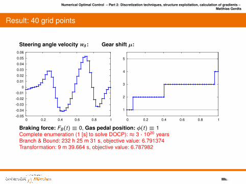
Numerical Optimal Control – Part 2: Discretization techniques, structure exploitation, calculation of gradients –Matthias Gerdts
Result: 40 grid points
Steering angle velocity wδ: Gear shift µ:
-0.05-0.04-0.03-0.02-0.01
0 0.01 0.02 0.03 0.04 0.05 0.06
0 0.2 0.4 0.6 0.8 1
1
2
3
4
5
0 0.2 0.4 0.6 0.8 1
Braking force: FB(t) ≡ 0, Gas pedal position: φ(t) ≡ 1Complete enumeration (1 [s] to solve DOCP):≈ 3 · 1020 yearsBranch & Bound: 232 h 25 m 31 s, objective value: 6.791374Transformation: 9 m 39.664 s, objective value: 6.787982
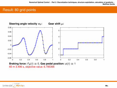
Numerical Optimal Control – Part 2: Discretization techniques, structure exploitation, calculation of gradients –Matthias Gerdts
Result: 80 grid points
Steering angle velocity wδ: Gear shift µ:
-0.06
-0.04
-0.02
0
0.02
0.04
0.06
0.08
0 0.2 0.4 0.6 0.8 1
1
2
3
4
5
0 0.2 0.4 0.6 0.8 1
Braking force: FB(t) ≡ 0, Gas pedal position: φ(t) ≡ 165 m 3.496 s, objective value: 6.795366
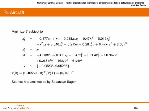
Numerical Optimal Control – Part 2: Discretization techniques, structure exploitation, calculation of gradients –Matthias Gerdts
F8 Aircraft
Minimize T subject to
x′1 = −0.877x1 + x3 − 0.088x1x3 + 0.47x21 − 0.019x2
2
−x21 x3 + 3.846x3
1 − 0.215v + 0.28x21 v + 0.47x1v2 + 0.63v3
x′2 = x3
x′3 = −4.208x1 − 0.396x3 − 0.47x21 − 3.564x3
1 − 20.967v
+6.265x21 v + 46x1v2 + 61.4v3
v ∈ −0.05236, 0.05236
x(0) = (0.4655, 0, 0)>, x(T ) = (0, 0, 0)>
Source: http://mintoc.de by Sebastian Sager
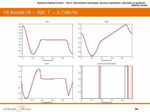
Numerical Optimal Control – Part 2: Discretization techniques, structure exploitation, calculation of gradients –Matthias Gerdts
F8 Aircraft (N = 500, T = 5.728674)
-0.05
0
0.05
0.1
0.15
0.2
0.25
0.3
0.35
0.4
0.45
0.5
0 0.2 0.4 0.6 0.8 1
normalized time
state 1
-0.5
-0.4
-0.3
-0.2
-0.1
0
0.1
0.2
0 0.2 0.4 0.6 0.8 1
normalized time
state 2
-0.6
-0.4
-0.2
0
0.2
0.4
0.6
0 0.2 0.4 0.6 0.8 1
normalized time
state 3
1
1.2
1.4
1.6
1.8
2
0 0.2 0.4 0.6 0.8 1
normalized time
control v (normalized values)
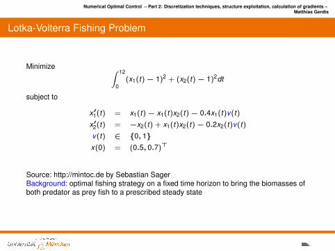
Numerical Optimal Control – Part 2: Discretization techniques, structure exploitation, calculation of gradients –Matthias Gerdts
Lotka-Volterra Fishing Problem
Minimize ∫ 12
0(x1(t)− 1)2 + (x2(t)− 1)2dt
subject to
x′1(t) = x1(t)− x1(t)x2(t)− 0.4x1(t)v(t)
x′2(t) = −x2(t) + x1(t)x2(t)− 0.2x2(t)v(t)
v(t) ∈ 0, 1x(0) = (0.5, 0.7)>
Source: http://mintoc.de by Sebastian SagerBackground: optimal fishing strategy on a fixed time horizon to bring the biomasses ofboth predator as prey fish to a prescribed steady state
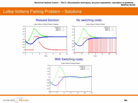
Numerical Optimal Control – Part 2: Discretization techniques, structure exploitation, calculation of gradients –Matthias Gerdts
Lotka-Volterra Fishing Problem – Solutions
Relaxed Solution: No switching costs:
-0.2
0
0.2
0.4
0.6
0.8
1
1.2
1.4
1.6
1.8
0 2 4 6 8 10 12
time t
Lotka-Volterra Fishing Problem (relaxed)
control v1state x1state x2
0
0.2
0.4
0.6
0.8
1
1.2
1.4
1.6
1.8
0 2 4 6 8 10 12
time t
Lotka-Volterra Fishing Problem
control v1state x1state x2
With Switching costs:
0
0.2
0.4
0.6
0.8
1
1.2
1.4
1.6
1.8
0 2 4 6 8 10 12
time t
Lotka-Volterra Fishing Problem
control v1statex1state x2
Numerical Optimal Control – Part 2: Discretization techniques, structure exploitation, calculation of gradients –Matthias Gerdts
References
[1] M. Gerdts.Solving Mixed-Integer Optimal Control Problems by Branch&Bound: A Case Study from Automobile Test-Driving with Gear Shift.Optimal Control, Applications and Methods, 26(1):1–18, 2005.
[2] M. Gerdts.A variable time transformation method for mixed-integer optimal control problems.Optimal Control, Applications and Methods, 27(3):169–182, 2006.
[3] S. Sager.Numerical methods for mixed-integer optimal control problems.PhD thesis, Naturwissenschaftlich-Mathematische Gesamtfakultat, Universitat Heidelberg, Heidelberg, Germany, 2006.
[4] S. Sager.MIOCP benchmark site. http://mintoc.de
[5] S. Sager, H. G. Bock, and G. Reinelt.Direct methods with maximal lower bound for mixed-integer optimal control problems.Mathematical Programming (A), 118(1):109–149, 2009.
[6] H. W. J. Lee, K. L. Teo, V. Rehbock, and L. S. Jennings.Control parametrization enhancing technique for optimal discrete-valued control problems.Automatica, 35(8):1401–1407, 1999.
[7] A. Siburian.Numerical Methods for Robust, Singular and Discrete Valued Optimal Control Problems.PhD thesis, Curtin University of Technology, Perth, Australia, 2004.
Numerical Optimal Control – Part 2: Discretization techniques, structure exploitation, calculation of gradients –Matthias Gerdts
Contents
Direct Discretization MethodsFull DiscretizationReduced Discretization and Shooting MethodsAdjoint EstimationConvergenceExamples
Mixed-Integer Optimal ControlVariable Time Transformation
Parametric Sensitivity Analysis and Realtime-OptimizationParametric Optimal Control Problems
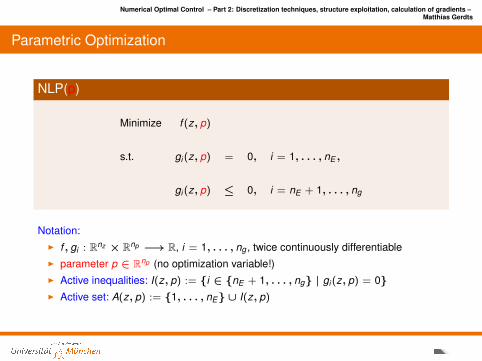
Numerical Optimal Control – Part 2: Discretization techniques, structure exploitation, calculation of gradients –Matthias Gerdts
Parametric Optimization
NLP(p)
Minimize f (z, p)
s.t. gi (z, p) = 0, i = 1, . . . , nE ,
gi (z, p) ≤ 0, i = nE + 1, . . . , ng
Notation:I f , gi : Rnz × Rnp −→ R, i = 1, . . . , ng , twice continuously differentiableI parameter p ∈ Rnp (no optimization variable!)I Active inequalities: I(z, p) := i ∈ nE + 1, . . . , ng | gi (z, p) = 0I Active set: A(z, p) := 1, . . . , nE ∪ I(z, p)
Numerical Optimal Control – Part 2: Discretization techniques, structure exploitation, calculation of gradients –Matthias Gerdts
Parametric Optimization
Definitionz∗ strongly regular local minimum of NLP(p0) iff
(a) z∗ is feasible.
(b) z∗ fulfills the linear independence constraint qualification (LICQ).
(c) The KKT conditions hold at (z∗, λ∗) with Lagrange multiplier λ∗.
(d) The strict complementarity condition holds:
λ∗i − gi (z∗, p0) > 0 for all i = nE + 1, . . . , ng .
(e) Second-order sufficient condition:
L′′zz (z∗, λ∗, p0)(d, d) > 0
for all 0 6= d ∈ TC(z∗, p0) with the critical cone
TC(z, p) :=
d ∈ Rnz
∣∣∣∣∣∣∣∣g′i,z (z, p)(d) ≤ 0, i ∈ I(z, p), λi = 0,
g′i,z (z, p)(d) = 0, i ∈ I(z, p), λi > 0,
g′i,z (z, p)(d) = 0, i ∈ 1, . . . , nE
.
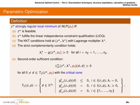
Numerical Optimal Control – Part 2: Discretization techniques, structure exploitation, calculation of gradients –Matthias Gerdts
Parametric Optimization
Sensitivity Theorem [Fiacco’83]Let z∗ be a strongly regular local minimum of (NLP(p0)) for nominal parameter p0.
Then there exist neighborhoods Bε(p0) and Bδ(z∗, λ∗) with:
I NLP(p) has unique strongly regular local minimum
(z(p), λ(p)) ∈ Bδ(z∗, λ∗)
for each p ∈ Bε(p0).I z(p), λ(p) are continuously differentiable w.r.t. p.I The active set remains unchanged for each p ∈ Bε(p0):
A(z∗, p0) = A(z(p), p).
Proof: implicit function theorem + stability of LICQ, critical cone and second-ordersufficient condition
Numerical Optimal Control – Part 2: Discretization techniques, structure exploitation, calculation of gradients –Matthias Gerdts
Parametric Optimization
Sensitivity Theorem [Fiacco’83]Let z∗ be a strongly regular local minimum of (NLP(p0)) for nominal parameter p0.
Then there exist neighborhoods Bε(p0) and Bδ(z∗, λ∗) with:I NLP(p) has unique strongly regular local minimum
(z(p), λ(p)) ∈ Bδ(z∗, λ∗)
for each p ∈ Bε(p0).
I z(p), λ(p) are continuously differentiable w.r.t. p.I The active set remains unchanged for each p ∈ Bε(p0):
A(z∗, p0) = A(z(p), p).
Proof: implicit function theorem + stability of LICQ, critical cone and second-ordersufficient condition
Numerical Optimal Control – Part 2: Discretization techniques, structure exploitation, calculation of gradients –Matthias Gerdts
Parametric Optimization
Sensitivity Theorem [Fiacco’83]Let z∗ be a strongly regular local minimum of (NLP(p0)) for nominal parameter p0.
Then there exist neighborhoods Bε(p0) and Bδ(z∗, λ∗) with:I NLP(p) has unique strongly regular local minimum
(z(p), λ(p)) ∈ Bδ(z∗, λ∗)
for each p ∈ Bε(p0).I z(p), λ(p) are continuously differentiable w.r.t. p.
I The active set remains unchanged for each p ∈ Bε(p0):
A(z∗, p0) = A(z(p), p).
Proof: implicit function theorem + stability of LICQ, critical cone and second-ordersufficient condition
Numerical Optimal Control – Part 2: Discretization techniques, structure exploitation, calculation of gradients –Matthias Gerdts
Parametric Optimization
Sensitivity Theorem [Fiacco’83]Let z∗ be a strongly regular local minimum of (NLP(p0)) for nominal parameter p0.
Then there exist neighborhoods Bε(p0) and Bδ(z∗, λ∗) with:I NLP(p) has unique strongly regular local minimum
(z(p), λ(p)) ∈ Bδ(z∗, λ∗)
for each p ∈ Bε(p0).I z(p), λ(p) are continuously differentiable w.r.t. p.I The active set remains unchanged for each p ∈ Bε(p0):
A(z∗, p0) = A(z(p), p).
Proof: implicit function theorem + stability of LICQ, critical cone and second-ordersufficient condition
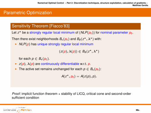
Numerical Optimal Control – Part 2: Discretization techniques, structure exploitation, calculation of gradients –Matthias Gerdts
Applications
I dependence of consistent initial values on parameters in DAEsI computation of gradients for bilevel optimization problems, e.g. Stackelberg
games, path planning under safety requirements (airraces)I parametric sensitivity analysis of reachable setsI model-predictive control: updates without re-optimization
see Vryan Palma’s talk Wednesday, September 11, 9:40 - 10:05
Numerical Optimal Control – Part 2: Discretization techniques, structure exploitation, calculation of gradients –Matthias Gerdts
Realtime Optimization [Buskens, Maurer]
Real-Time Approximation for NLP(p)Given: (offline)
I nominal parameter p0
I strongly regular local minimum z∗
I sensitivity differentials dzdp (p0)
Taylor approximation/real-time approximation: (online)For a perturbed parameter p 6= p0 compute
z(p) := z(p0) +dzdp
(p0)(p − p0)
and use z(p) as an approximation of z(p).
Limitations:
I approximation error ‖z(p)− z(p)‖ = o(‖p − p0‖)I constraint violation due to linearization (projection required if feasibility is an issue)I linearization only justified in neighborhood Bε(p0), same active set
Numerical Optimal Control – Part 2: Discretization techniques, structure exploitation, calculation of gradients –Matthias Gerdts
Realtime Optimization [Buskens, Maurer]
Real-Time Approximation for NLP(p)Given: (offline)
I nominal parameter p0
I strongly regular local minimum z∗
I sensitivity differentials dzdp (p0)
Taylor approximation/real-time approximation: (online)For a perturbed parameter p 6= p0 compute
z(p) := z(p0) +dzdp
(p0)(p − p0)
and use z(p) as an approximation of z(p).
Limitations:I approximation error ‖z(p)− z(p)‖ = o(‖p − p0‖)
I constraint violation due to linearization (projection required if feasibility is an issue)I linearization only justified in neighborhood Bε(p0), same active set
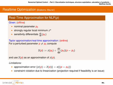
Numerical Optimal Control – Part 2: Discretization techniques, structure exploitation, calculation of gradients –Matthias Gerdts
Realtime Optimization [Buskens, Maurer]
Real-Time Approximation for NLP(p)Given: (offline)
I nominal parameter p0
I strongly regular local minimum z∗
I sensitivity differentials dzdp (p0)
Taylor approximation/real-time approximation: (online)For a perturbed parameter p 6= p0 compute
z(p) := z(p0) +dzdp
(p0)(p − p0)
and use z(p) as an approximation of z(p).
Limitations:I approximation error ‖z(p)− z(p)‖ = o(‖p − p0‖)I constraint violation due to linearization (projection required if feasibility is an issue)
I linearization only justified in neighborhood Bε(p0), same active set
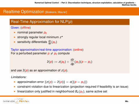
Numerical Optimal Control – Part 2: Discretization techniques, structure exploitation, calculation of gradients –Matthias Gerdts
Realtime Optimization [Buskens, Maurer]
Real-Time Approximation for NLP(p)Given: (offline)
I nominal parameter p0
I strongly regular local minimum z∗
I sensitivity differentials dzdp (p0)
Taylor approximation/real-time approximation: (online)For a perturbed parameter p 6= p0 compute
z(p) := z(p0) +dzdp
(p0)(p − p0)
and use z(p) as an approximation of z(p).
Limitations:I approximation error ‖z(p)− z(p)‖ = o(‖p − p0‖)I constraint violation due to linearization (projection required if feasibility is an issue)I linearization only justified in neighborhood Bε(p0), same active set
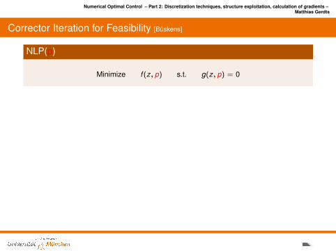
Numerical Optimal Control – Part 2: Discretization techniques, structure exploitation, calculation of gradients –Matthias Gerdts
Corrector Iteration for Feasibility [Buskens]
NLP(p)
Minimize f (z, p) s.t. g(z, p) = 0
Realtime approximation:
z [0](p) := z(p) = z(p0) +dzdp
(p0)(p − p0)
Introducing z(p) into constraints yields constraint violation
ε[0] := g(z(p), p)
Idea of corrector iteration:
I perform sensitivity analysis w.r.t. ε for nominal parameter ε0 = 0I apply correction (fixed point iteration):
z [i+1](p) := z [i](p)−dzdε
(p0, ε0)ε[i], ε[i] := g(z [i](p), p)
(note the minus sign!)
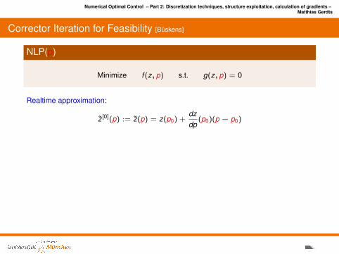
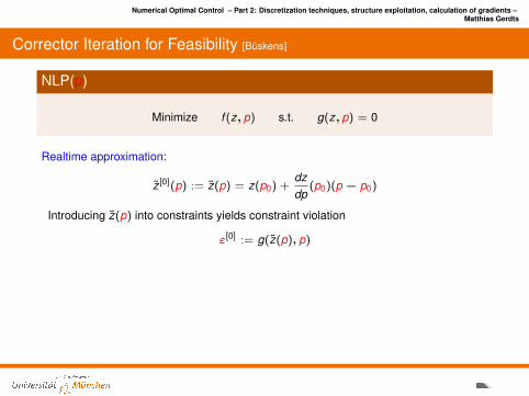
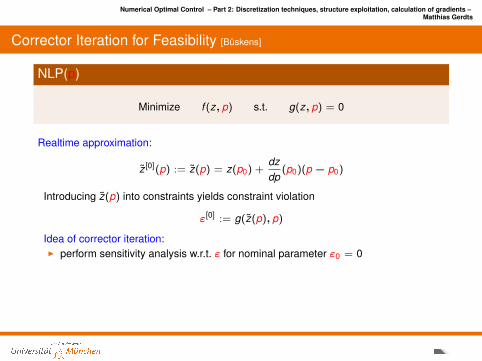
Numerical Optimal Control – Part 2: Discretization techniques, structure exploitation, calculation of gradients –Matthias Gerdts
Corrector Iteration for Feasibility [Buskens]
NLP(p)
Minimize f (z, p) s.t. g(z, p) = 0
Realtime approximation:
z [0](p) := z(p) = z(p0) +dzdp
(p0)(p − p0)
Introducing z(p) into constraints yields constraint violation
ε[0] := g(z(p), p)
Idea of corrector iteration:I perform sensitivity analysis w.r.t. ε for nominal parameter ε0 = 0
I apply correction (fixed point iteration):
z [i+1](p) := z [i](p)−dzdε
(p0, ε0)ε[i], ε[i] := g(z [i](p), p)
(note the minus sign!)
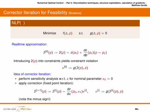
Numerical Optimal Control – Part 2: Discretization techniques, structure exploitation, calculation of gradients –Matthias Gerdts
Corrector Iteration for Feasibility [Buskens]
NLP(p)
Minimize f (z, p) s.t. g(z, p) = 0
Realtime approximation:
z [0](p) := z(p) = z(p0) +dzdp
(p0)(p − p0)
Introducing z(p) into constraints yields constraint violation
ε[0] := g(z(p), p)
Idea of corrector iteration:I perform sensitivity analysis w.r.t. ε for nominal parameter ε0 = 0I apply correction (fixed point iteration):
z [i+1](p) := z [i](p)−dzdε
(p0, ε0)ε[i], ε[i] := g(z [i](p), p)
(note the minus sign!)
Numerical Optimal Control – Part 2: Discretization techniques, structure exploitation, calculation of gradients –Matthias Gerdts
Contents
Direct Discretization MethodsFull DiscretizationReduced Discretization and Shooting MethodsAdjoint EstimationConvergenceExamples
Mixed-Integer Optimal ControlVariable Time Transformation
Parametric Sensitivity Analysis and Realtime-OptimizationParametric Optimal Control Problems
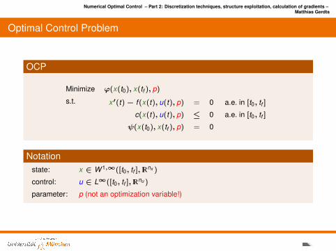
Numerical Optimal Control – Part 2: Discretization techniques, structure exploitation, calculation of gradients –Matthias Gerdts
Optimal Control Problem
OCP
Minimize ϕ(x(t0), x(tf ), p)
s.t. x′(t)− f (x(t), u(t), p) = 0 a.e. in [t0, tf ]
c(x(t), u(t), p) ≤ 0 a.e. in [t0, tf ]
ψ(x(t0), x(tf ), p) = 0
Notationstate: x ∈ W 1,∞([t0, tf ], IRnx )
control: u ∈ L∞([t0, tf ], IRnu )
parameter: p (not an optimization variable!)
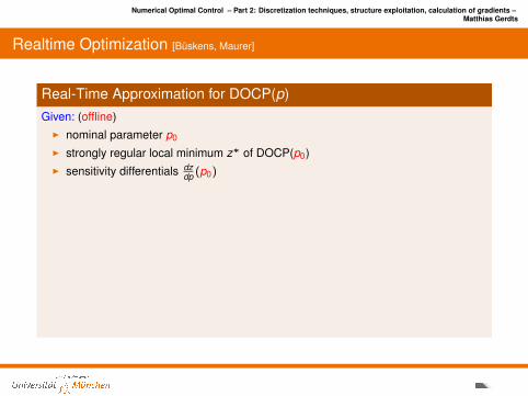
Numerical Optimal Control – Part 2: Discretization techniques, structure exploitation, calculation of gradients –Matthias Gerdts
Realtime Optimization [Buskens, Maurer]
Real-Time Approximation for DOCP(p)Given: (offline)
I nominal parameter p0
I strongly regular local minimum z∗ of DOCP(p0)I sensitivity differentials dz
dp (p0)
Taylor approximation/real-time approximation: (online)For a perturbed parameter p 6= p0 compute
x1(p) := x1(p) +dx1
dp(p0)(p − p0),
ui (p) := ui (p0) +dui
dp(p0)(p − p0).
and use x1(p) as an approximation of the initial value x1(p) and ui (p) as anapproximate optimal control for the parameter p.
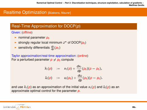
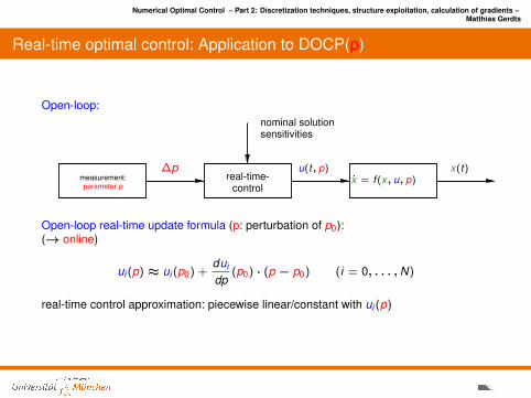
Numerical Optimal Control – Part 2: Discretization techniques, structure exploitation, calculation of gradients –Matthias Gerdts
Real-time optimal control: Application to DOCP(p)
Open-loop:
measurement:parameter p
∆preal-time-
control
u(t, p)x = f (x, u, p)
x(t)
nominal solutionsensitivities
Open-loop real-time update formula (p: perturbation of p0):(→ online)
ui (p) ≈ ui (p0) +dui
dp(p0) · (p − p0) (i = 0, . . . ,N)
real-time control approximation: piecewise linear/constant with ui (p)
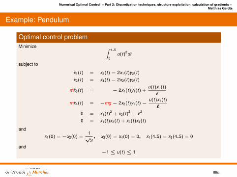
Numerical Optimal Control – Part 2: Discretization techniques, structure exploitation, calculation of gradients –Matthias Gerdts
Example: Pendulum
Optimal control problemMinimize ∫ 4.5
0u(t)2dt
subject to
x1(t) = x3(t)− 2x1(t)y2(t)
x2(t) = x4(t)− 2x2(t)y2(t)
mx3(t) = − 2x1(t)y1(t) +u(t)x2(t)`
mx4(t) = −mg − 2x2(t)y1(t)−u(t)x1(t)`
0 = x1(t)2 + x2(t)2 − `2
0 = x1(t)x3(t) + x2(t)x4(t)
and
x1(0) = −x2(0) =1√
2, x3(0) = x4(0) = 0, x1(4.5) = x3(4.5) = 0
and−1 ≤ u(t) ≤ 1
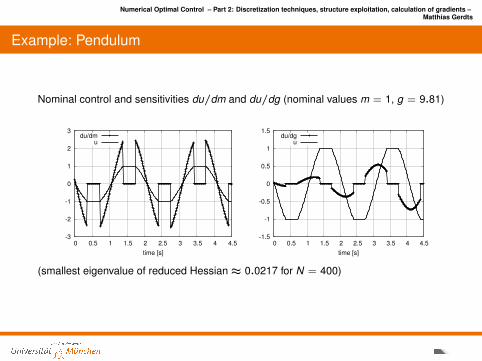
Numerical Optimal Control – Part 2: Discretization techniques, structure exploitation, calculation of gradients –Matthias Gerdts
Example: Pendulum
Nominal control and sensitivities du/dm and du/dg (nominal values m = 1, g = 9.81)
-3
-2
-1
0
1
2
3
0 0.5 1 1.5 2 2.5 3 3.5 4 4.5
time [s]
du/dmu
-1.5
-1
-0.5
0
0.5
1
1.5
0 0.5 1 1.5 2 2.5 3 3.5 4 4.5
time [s]
du/dgu
(smallest eigenvalue of reduced Hessian≈ 0.0217 for N = 400)
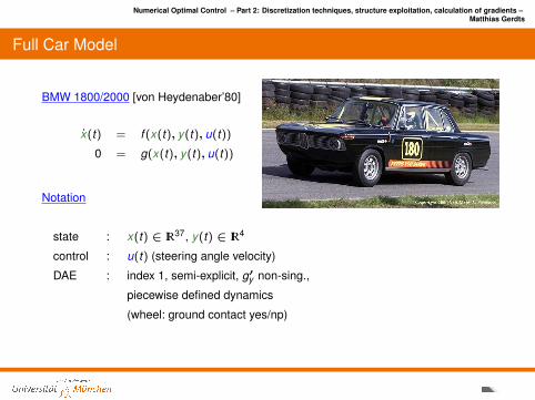
Numerical Optimal Control – Part 2: Discretization techniques, structure exploitation, calculation of gradients –Matthias Gerdts
Full Car Model
BMW 1800/2000 [von Heydenaber’80]
x(t) = f (x(t), y(t), u(t))
0 = g(x(t), y(t), u(t))
Notation
state : x(t) ∈ IR37, y(t) ∈ IR4
control : u(t) (steering angle velocity)
DAE : index 1, semi-explicit, g′y non-sing.,
piecewise defined dynamics
(wheel: ground contact yes/np)
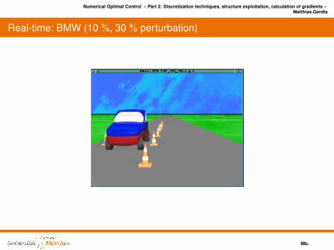
Numerical Optimal Control – Part 2: Discretization techniques, structure exploitation, calculation of gradients –Matthias Gerdts
Real-time: BMW (10 %, 30 % perturbation)
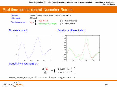
Numerical Optimal Control – Part 2: Discretization techniques, structure exploitation, calculation of gradients –Matthias Gerdts
Real-time optimal control: Numerical ResultsObjective: linear combination of final time and steering effort→ min
Initial velocity: 25 [m/s]
Real-time parameter: p0 =
offset 3.5 [m] (→ state constraints)
centre of gravity 0.56 [m] (→ car’s dynamics)
Nominal control:
-1
-0.5
0
0.5
1
1.5
0 0.2 0.4 0.6 0.8 1
Sensitivity differentials u:
-0.6
-0.4
-0.2
0
0.2
0.4
0.6
0.8
1
1.2
1.4
0 0.2 0.4 0.6 0.8 1
Sensitivity differentials tf :
dtf (p0)
dp=
(0.4683 · 10−1
0.2574 · 10−1
)Accuracy: Optimality/feasibility 10−11, DSRTSE (10−11 diff, 10−4 alg), N = 81, M = 1
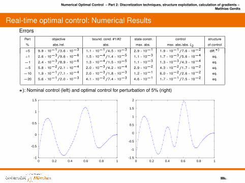
Numerical Optimal Control – Part 2: Discretization techniques, structure exploitation, calculation of gradients –Matthias Gerdts
Real-time optimal control: Numerical ResultsErrors
Pert objective bound. cond. #1/#2 state constr. control structure
% abs./rel. abs. max. abs. max. abs./abs. L2 of control
+5 9.9 · 10−1/3.6 · 10−3 1.1 · 10−1/4.5 · 10−3 2.9 · 10−1 1.9 · 10−1/7.6 · 10−2 diff.∗)
+1 2.6 · 10−3/9.6 · 10−6 1.5 · 10−4/1.4 · 10−5 1.1 · 10−3 1.7 · 10−3/5.6 · 10−4 eq.
−1 2.4 · 10−3/8.9 · 10−6 1.3 · 10−4/1.5 · 10−5 1.1 · 10−3 1.3 · 10−3/4.3 · 10−4 eq.
−5 5.8 · 10−2/2.1 · 10−4 2.0 · 10−3/4.2 · 10−4 2.9 · 10−2 4.3 · 10−2/1.7 · 10−2 eq.
−10 1.9 · 10−1/7.1 · 10−4 2.0 · 10−3/1.8 · 10−3 1.2 · 10−1 6.0 · 10−2/2.6 · 10−2 eq.
−20 5.6 · 10−1/2.0 · 10−3 4.1 · 10−2/7.4 · 10−3 4.6 · 10−1 1.7 · 10−1/7.5 · 10−2 eq.
∗): Nominal control (left) and optimal control for perturbation of 5% (right)
-1
-0.5
0
0.5
1
1.5
0 0.2 0.4 0.6 0.8 1-1.5
-1
-0.5
0
0.5
1
1.5
2
0 0.2 0.4 0.6 0.8 1
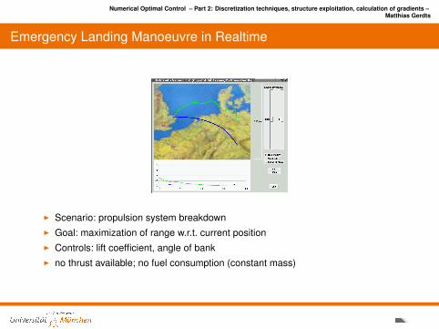
Numerical Optimal Control – Part 2: Discretization techniques, structure exploitation, calculation of gradients –Matthias Gerdts
Emergency Landing Manoeuvre in Realtime
I Scenario: propulsion system breakdownI Goal: maximization of range w.r.t. current positionI Controls: lift coefficient, angle of bankI no thrust available; no fuel consumption (constant mass)
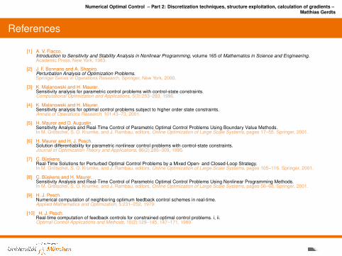
Numerical Optimal Control – Part 2: Discretization techniques, structure exploitation, calculation of gradients –Matthias Gerdts
References
[1] A. V. Fiacco.Introduction to Sensitivity and Stability Analysis in Nonlinear Programming, volume 165 of Mathematics in Science and Engineering.Academic Press, New York, 1983.
[2] J. F. Bonnans and A. Shapiro.Perturbation Analysis of Optimization Problems.Springer Series in Operations Research. Springer, New York, 2000.
[3] K. Malanowski and H. Maurer.Sensitivity analysis for parametric control problems with control-state constraints.Computational Optimization and Applications, 5(3):253–283, 1996.
[4] K. Malanowski and H. Maurer.Sensitivity analysis for optimal control problems subject to higher order state constraints.Annals of Operations Research, 101:43–73, 2001.
[5] H. Maurer and D. Augustin.Sensitivity Analysis and Real-Time Control of Parametric Optimal Control Problems Using Boundary Value Methods.In M. Grotschel, S. O. Krumke, and J. Rambau, editors, Online Optimization of Large Scale Systems, pages 17–55. Springer, 2001.
[6] H. Maurer and H. J. Pesch.Solution differentiability for parametric nonlinear control problems with control-state constraints.Journal of Optimization Theory and Applications, 86(2):285–309, 1995.
[7] C. Buskens.Real-Time Solutions for Perturbed Optimal Control Problems by a Mixed Open- and Closed-Loop Strategy.In M. Grotschel, S. O. Krumke, and J. Rambau, editors, Online Optimization of Large Scale Systems, pages 105–116. Springer, 2001.
[8] C. Buskens and H. Maurer.Sensitivity Analysis and Real-Time Control of Parametric Optimal Control Problems Using Nonlinear Programming Methods.In M. Grotschel, S. O. Krumke, and J. Rambau, editors, Online Optimization of Large Scale Systems, pages 56–68. Springer, 2001.
[9] H. J. Pesch.Numerical computation of neighboring optimum feedback control schemes in real-time.Applied Mathematics and Optimization, 5:231–252, 1979.
[10] H. J. Pesch.Real-time computation of feedback controls for constrained optimal control problems. i, ii.Optimal Control Applications and Methods, 10(2):129–145, 147–171, 1989.
Numerical Optimal Control – Part 2: Discretization techniques, structure exploitation, calculation of gradients –Matthias Gerdts
References
J. T. Betts.Practical methods for optimal control using nonlinear programming, volume 3 ofAdvances in Design and Control.SIAM, Philadelphia, 2001.
M. Gerdts.Optimal Control of ODEs and DAEs.DeGruyter, Berlin, 2011
Numerical Optimal Control – Part 2: Discretization techniques, structure exploitation, calculation of gradients –Matthias Gerdts
Thanks for your Attention!
Questions?
Further information:
[email protected]/lrt1/gerdtswww.optimal-control.de
Fotos: http://de.wikipedia.org/wiki/MunchenMagnus Manske (Panorama), Luidger (Theatinerkirche), Kurmis (Chin. Turm), Arad Mojtahedi (Olympiapark), Max-k (Deutsches Museum), Oliver Raupach (Friedensengel), Andreas Praefcke (Nationaltheater)


![OptimalControlofthe Convection-Diffusion … · 2015. 10. 7. · optimal control problems with pointwise inequality constraints, we refer e.g. to [1, 10, 14, 20]. In [24] discretization](https://img.pdfslide.net/doc/110x75/607223d055e1586fab3d8511/optimalcontrolofthe-convection-diiusion-2015-10-7-optimal-control-problems.jpg)