Numerical Performance Prediction of a Miniature at Mach 4

Calhoun: The NPS Institutional Archive

Theses and Dissertations Thesis and Dissertation Collection

2012-09

Numerical Performance Prediction of a Miniature at

Mach 4

Chen, Bingqiang

Monterey, California. Naval Postgraduate School

http://hdl.handle.net/10945/17340

NAVAL

POSTGRADUATE SCHOOL

MONTEREY, CALIFORNIA

THESIS

Approved for public release; distribution is unlimited

NUMERICAL PERFORMANCE PREDICTION OF A MINIATURE RAMJET AT MACH 4

by

Bingqiang Chen

September 2012

Thesis Advisor: Garth V. Hobson Second Reader: Christopher M. Brophy

THIS PAGE INTENTIONALLY LEFT BLANK

i

REPORT DOCUMENTATION PAGE Form Approved OMB No. 0704-0188

Public reporting burden for this collection of information is estimated to average 1 hour per response, including the time for reviewing instruction, searching existing data sources, gathering and maintaining the data needed, and completing and reviewing the collection of information. Send comments regarding this burden estimate or any other aspect of this collection of information, including suggestions for reducing this burden, to Washington headquarters Services, Directorate for Information Operations and Reports, 1215 Jefferson Davis Highway, Suite 1204, Arlington, VA 22202-4302, and to the Office of Management and Budget, Paperwork Reduction Project (0704-0188) Washington DC 20503. 1. AGENCY USE ONLY (Leave blank)

2. REPORT DATE September 2012

3. REPORT TYPE AND DATES COVERED Master’s Thesis

4. TITLE AND SUBTITLE Numerical Performance Prediction of a Miniature at Mach 4

5. FUNDING NUMBERS

6. AUTHOR(S) Bingqiang Chen

7. PERFORMING ORGANIZATION NAME(S) AND ADDRESS(ES)Naval Postgraduate School Monterey, CA 93943-5000

8. PERFORMING ORGANIZATION REPORT NUMBER

9. SPONSORING /MONITORING AGENCY NAME(S) AND ADDRESS(ES)N/A

10. SPONSORING/MONITORING AGENCY REPORT NUMBER

11. SUPPLEMENTARY NOTES The views expressed in this thesis are those of the author and do not reflect the official policy or position of the Department of Defense or the U.S. Government.

12a. DISTRIBUTION / AVAILABILITY STATEMENT Approved for public release; distribution is unlimited.

12b. DISTRIBUTION CODE A

13. ABSTRACT (maximum 200 words) Using a 3-D axis-symmetric model, the cold-flow performance of a miniature ramjet in Mach 4 flow was predicted with the computational fluids dynamic (CFD) code from ANSYS-CFX. The nozzle-throat area was varied to increase the backpressure and this pushed the normal shock that was sitting within the inlet, out to the lip of the inlet cowl.

Using the eddy dissipation combustion model in ANSYS-CFX, a combustion analysis was performed on the miniature ramjet. The analysis involved the single-step, stoichiometric combustion of hydrogen and oxygen within the combustion chamber of the ramjet.

The drag force induced on the miniature ramjet when subjected to Mach 4 flow in a supersonic wind tunnel was measured using cryogenic strain gauges arranged in a Wheatstone bridge. A CFD cold-flow drag prediction was compared against this measured drag force to establish the former’s accuracy in drag prediction.

For all CFD predictions, the two-equation Shear-Stress-Transport (SST) turbulence model was used. The SST turbulence model blends the k-epsilon and k-omega turbulence model and effects the transportation of the turbulent shear stress for improved accuracy in turbulence modeling.

14. SUBJECT TERMS Mach 4, Ramjet, Drag, Turbulence Modeling, Simulation, ANSYS CFX

15. NUMBER OF PAGES

131 16. PRICE CODE

17. SECURITY CLASSIFICATION OF REPORT

Unclassified

18. SECURITY CLASSIFICATION OF THIS PAGE

Unclassified

19. SECURITY CLASSIFICATION OF ABSTRACT

Unclassified

20. LIMITATION OF ABSTRACT

UU NSN 7540-01-280-5500 Standard Form 298 (Rev. 8-98) Prescribed by ANSI Std. Z39.18

ii


iii

Approved for public release; distribution is unlimited

NUMERICAL PERFORMANCE PREDICTION OF A MINIATURE RAMJET AT MACH 4

Bingqiang Chen Major, Singapore Armed Forces

B.Eng., Nanyang Technological University, 2007

Submitted in partial fulfillment of the requirements for the degree of

MASTER OF SCIENCE IN ENGINEERING SCIENCE (MECHANICAL ENGINEERING)

from the

NAVAL POSTGRADUATE SCHOOL September 2012

Author: Bingqiang Chen

Approved by: Garth V. Hobson Thesis Advisor

Christopher M. Brophy Second Reader

Knox T. Milsaps Chair, Department of Mechanical and Aerospace Engineering

iv


v

ABSTRACT

Using a 3-D axis-symmetric model, the cold-flow performance of a miniature

ramjet in Mach 4 flow was predicted with the computational fluids dynamic (CFD) code

from ANSYS-CFX. The nozzle-throat area was varied to increase the backpressure and

this pushed the normal shock that was sitting within the inlet, out to the lip of the inlet

cowl.

Using the eddy dissipation combustion model in ANSYS-CFX, a combustion

analysis was performed on the miniature ramjet. The analysis involved the single-step,

stoichiometric combustion of hydrogen and oxygen within the combustion chamber of the

ramjet.

The drag force induced on the miniature ramjet when subjected to Mach 4 flow in

a supersonic wind tunnel was measured using cryogenic strain gauges arranged in a

Wheatstone bridge. A CFD cold-flow drag prediction was compared against this

measured drag force to establish the former’s accuracy in drag prediction.

For all CFD predictions, the two-equation Shear-Stress-Transport (SST)

turbulence model was used. The SST turbulence model blends the k-epsilon and k-

omega turbulence model and effects the transportation of the turbulent shear stress for

improved accuracy in turbulence modeling.

vi


vii

TABLE OF CONTENTS

I. INTRODUCTION .................................................................................................... 1

II. NUMERICAL PERFORMANCE PREDICTION WITH ANSYS-CFX ...................... 3 A. ANSYS-CFX ................................................................................................ 3 B. TURBULENCE MODELLING ...................................................................... 3 C. COMBUSTION MODELING ........................................................................ 5 D. RAMJET NOMENCLATURE ....................................................................... 6

III. COLD-FLOW CFD ANALYSIS .............................................................................. 7 A. BACKGROUND AND METHODOLOGY .................................................... 7 B. COMPUTATIONAL MODEL SETUP FOR COLD-FLOW ANALYSES ....... 8

1. Three-Dimensional Computational Model..................................... 8 2. Boundary Conditions and Key Simulation-Setup

Parameters ...................................................................................... 9 C. RESULTS AND DISCUSSION .................................................................. 10

1. Flow-Profile Comparison .............................................................. 10 2. Results of Cold-Flow Analysis with Varied Nozzle-Throat

Area ................................................................................................ 14

IV. CFD ANALYSIS FOR AIR INJECTION THROUGH THE TIP PORTS ................ 17 A. BACKGROUND AND METHODOLOGY .................................................. 17 B. COMPUTATIONAL MODEL SETUP ......................................................... 17

1. Three-Dimensional Model Setup .................................................. 17 2. Boundary Conditions and Key Simulation-Setup

Parameters .................................................................................... 18 C. RESULTS AND DISCUSSION .................................................................. 19

V. COMBUSTION CFD ANALYSIS .......................................................................... 23 A. BACKGROUND AND METHODOLOGY .................................................. 23 B. COMPUTATIONAL MODEL SETUP FOR MIXING-FLOW ANALYSIS .... 23

1. Three-Dimensional Model Setup .................................................. 23 2. Boundary Conditions and Key Simulation-Setup

Parameters .................................................................................... 25 C. RESULTS AND DISCUSSION .................................................................. 25

V. SUPERSONIC WIND-TUNNEL EXPERIMENT AND COMPARISON WITH CFD ...................................................................................................................... 29 A. BACKGROUND AND METHODOLOGY .................................................. 29 B. EXPERIMENTAL SETUP .......................................................................... 30

1. New Ramjet Model with Shortened Flexures .............................. 30 2. Strain Gauges and Wiring ............................................................ 32 4. Signals Conditioning System ....................................................... 32 5. Data Acquisition System .............................................................. 33

C. PROCEDURES ......................................................................................... 34 D. CFD DRAG PREDICTION ......................................................................... 34 E. RESULTS AND DISCUSSION .................................................................. 36

viii

1. SSWT Experiment ......................................................................... 36 2. CFD Drag Prediction ..................................................................... 36 3. Discussion ..................................................................................... 37

VII. CONCLUSIONS AND RECOMMENDATIONS .................................................... 41

APPENDIX A – DETAIL SETUP FOR COLD-FLOW ANALYSIS .................................. 43 A1. MESH SETUP ........................................................................................... 43 A2. CFX-PRE SETUP PARAMETERS ............................................................ 45 A3. OTHER NOTES ......................................................................................... 50

APPENDIX B – RESULTS FOR COLD-FLOW CFD ANALYSES ................................. 51 B1. MACH NUMBER PROFILE ....................................................................... 51 B2. PRESSURE PROFILE ............................................................................... 52 B3. DENSITY PROFILE ................................................................................... 53 B4. STREAMLINE PLOT ................................................................................. 54 B5. SHOCK INDICATOR PLOT ...................................................................... 55 B6. DRAG COEFFICIENT COMPUTATION .................................................... 56

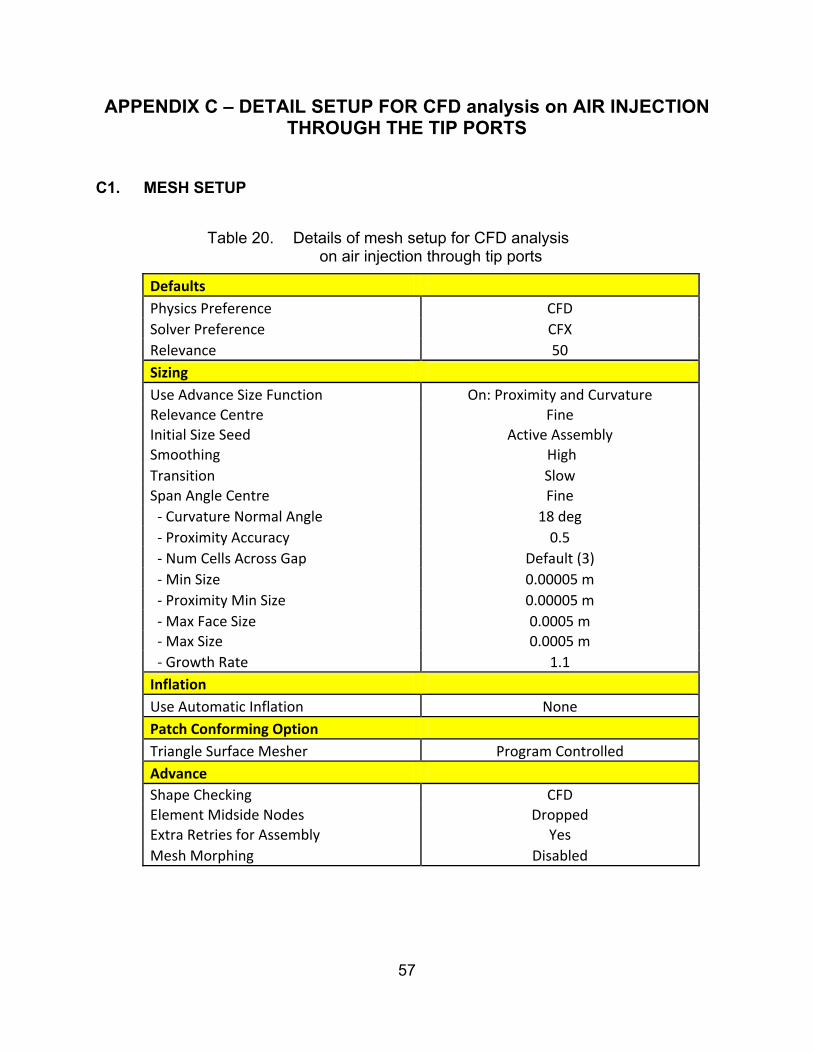
APPENDIX C – DETAIL SETUP FOR CFD ANALYSIS ON AIR INJECTION THROUGH THE TIP PORTS ............................................................................... 57 C1. MESH SETUP ........................................................................................... 57 C2. CFX-PRE SETUP PARAMETERS ............................................................ 59 C3. OTHER NOTES ......................................................................................... 66

APPENDIX D – RESULTS FOR CFD ANALYSIS ON AIR INJECTION THROUGH THE TIP PORTS .................................................................................................. 67 D1. VELOCITY STREAMLINES ...................................................................... 67 D2. MACH NUMBER PROFILE ....................................................................... 68 D3. ISO-SURFACE PLOT FOR MACH 3.65 ................................................... 69

APPENDIX E – STOICHIOMETRIC CALCULATION ..................................................... 71 E1. STOICHIOMETRIC FUEL-AIR RATIO ...................................................... 71 E2. REQUIRED MASS FLOW FOR HYDROGEN ........................................... 72

APPENDIX F – DETAIL SETUP FOR COMBUSTION CFD ANALYSIS ........................ 73 F1. MESH SETUP ........................................................................................... 73 F2. CFX-PRE SETUP PARAMETERS ............................................................ 75 F3. OTHER NOTES ......................................................................................... 82

APPENDIX G – ENGINEERING DRAWINGS FOR RAMJET MODEL .......................... 83

APPENDIX H – DETAILS FOR STRAIN GAUGES USED ............................................. 97

APPENDIX I – DETAILED EXPERIMENT PROCEDURES FOR DRAG MEASUREMENT EXPERIMENT ......................................................................... 99 I1. CALIBRATION OF SIGNALS CONDITIONING SYSTEM ........................ 99 I2. LOAD CELL CALIBRATION ................................................................... 100 I3. STRAIN GAUGE CALIBRATION ............................................................ 100 I4. DRAG MEASUREMENT ......................................................................... 102

APPENDIX J – DETAIL SETUP FOR CFD DRAG PREDICTION ................................ 105 J1. MESH SETUP ......................................................................................... 105

ix

J2. CFX-PRE SETUP PARAMETERS .......................................................... 105 J3. OTHER NOTES ....................................................................................... 107

LIST OF REFERENCES ............................................................................................... 109

INITIAL DISTRIBUTION LIST ...................................................................................... 111

x


xi

LIST OF FIGURES

Figure 1. Schematic of ramjet with associated stations .............................................. 6 Figure 2. Geometry of ramjet with two axes of symmetry ........................................... 8 Figure 3. Three-dimensional computational model for cold-flow analysis, with

boundary namespace .................................................................................. 8 Figure 4. Mesh of computation model for cold-flow analysis ....................................... 9 Figure 5. Mach number distribution with ANSYS-CFX .............................................. 10 Figure 6. Mach number distribution with Overflow code [1] ...................................... 11 Figure 7. Mach number distribution with CFDRC-FASTRAN [2] ............................... 11 Figure 8. Pressure distribution with ANSYS-CFX ..................................................... 11 Figure 9. Density distribution with ANSYS-CFX ........................................................ 12 Figure 10. Temperature distribution with ANSYS-CFX ............................................... 12 Figure 11. Streamline plot with ANSYS-CFX .............................................................. 12 Figure 12. Cold-flow shock profile with 10% reduction in nozzle-throat area .............. 14 Figure 13. Cold-flow shock profile with 20% reduction in nozzle-throat area .............. 14 Figure 14. Cold-flow shock profile with 30% reduction in nozzle-throat area .............. 14 Figure 15. Cold-flow shock profile with 40% reduction in nozzle-throat area .............. 15 Figure 16. Shock indicator around inlet for a) 10% b) 20%, c) 30%, d) 30%

reduction in throat area .............................................................................. 15 Figure 17. Three-dimensional geometry of computational model for air injection

analysis, with boundary namespace .......................................................... 18 Figure 18. Mesh of computational model for air injection analysis .............................. 18 Figure 19. Mach number distribution for air injection through tip port with Pt = 0.5

atm ............................................................................................................. 19 Figure 20. Mach number distribution for air injection through tip port with Pt = 0.75

atm ............................................................................................................. 20 Figure 21. Mach number distribution for air injection through tip port with Pt = 1

atm ............................................................................................................. 20 Figure 22. Iso-surface plot of Mach 3.65, for air injection through tip port with Pt =

0.5 atm ....................................................................................................... 21 Figure 23. Three-dimensional geometry of computational model for combustion

analysis, with boundary namespace .......................................................... 24 Figure 24. Mesh of computational model for mixing analysis ...................................... 24 Figure 25. RMS convergence history with reference time step for hydrogen

injection ...................................................................................................... 26 Figure 26. Temperature distribution for fuel injection at each reference location ........ 27 Figure 27. Top-down schematic of ramjet in SSWT .................................................... 30 Figure 28. Comparison of center-body (partial) and strut dimensioning ...................... 30 Figure 29. Assembled new ramjet model .................................................................... 31 Figure 30. Assembled ramjet model mounted in the SSWT ....................................... 31 Figure 31. Wheatstone bridge for potential difference measurements ........................ 32 Figure 32. Signals-conditioning system ...................................................................... 33 Figure 33. Measurement Computing USB-1698FS-Plus data acquisition (DAQ)

module ....................................................................................................... 33

xii

Figure 34. 3-D computational model for cold-flow drag analysis, with boundary namespace ................................................................................................ 35

Figure 35. Comparison of (a) Physical flexure model and (b) Equivalent CFD flexure model ............................................................................................. 35

Figure 36. Schlieren image of ramjet in SSWT at Mach 4 conditions ......................... 36 Figure 37. Calibration setup of load cell and thrust fixture in SSWT ........................... 39 Figure 38. Part drawing: Ramjet inlet nose cone (RJ – 1) ........................................... 83 Figure 39. Part drawing: Ramjet center body (RJ – 2 – 1) .......................................... 84 Figure 40. Part drawing: Contour of ramjet center body (RJ – 2 – 2) .......................... 85 Figure 41. Part drawing: Ramjet horizontal struts (RJ – 3 – 1) ................................... 86 Figure 42. Part drawing: Ramjet horizontal struts (RJ – 3 – 2) ................................... 87 Figure 43. Part drawing: Ramjet vertical struts (RJ – 4 – 1) ........................................ 88 Figure 44. Part drawing: Ramjet vertical struts (RJ – 4 – 2) ........................................ 89 Figure 45. Part drawing: Ramjet intake (RJ – 5) ......................................................... 90 Figure 46. Part drawing: Ramjet combustion chamber (RJ – 6) ................................. 91 Figure 47. Part drawing: Ramjet nozzle (RJ – 7) ........................................................ 92 Figure 48. Part drawing: Flexure (RJ – 8 – 1) ............................................................. 93 Figure 49. Part drawing: Flexure (RJ – 8 – 2) ............................................................. 94 Figure 50. Part drawing: Flexure (RJ – 8 – 3) ............................................................. 95 Figure 51. Wiring diagram for load cell calibration .................................................... 100 Figure 52. Wiring diagram for bridge balancing ........................................................ 101 Figure 53. Load cell and thrust fixture mounted in SSWT with ramjet model ............ 102

xiii

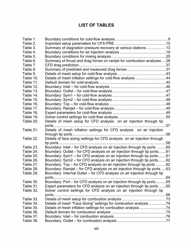
LIST OF TABLES

Table 1. Boundary conditions for cold-flow analysis. ................................................. 9 Table 2. Important setup parameters for CFX-PRE. ................................................ 10 Table 3. Summary of stagnation pressure recovery at various stations ................... 13 Table 4. Boundary conditions for air injection analysis ............................................ 19 Table 5. Boundary conditions for mixing analysis .................................................... 25 Table 6. Summary of thrust and drag forces on ramjet for combustion analyses .... 28 Table 7. CFD drag prediction ................................................................................... 37 Table 8. Summary of predicted and measured drag forces ..................................... 37 Table 9. Details of mesh setup for cold-flow analysis .............................................. 43 Table 10. Details of mesh inflation settings for cold-flow analysis ............................. 44 Table 11. Default domain for cold-analysis ................................................................ 45 Table 12. Boundary: Inlet – for cold-flow analysis...................................................... 46 Table 13. Boundary: Outlet – for cold-flow analysis ................................................... 47 Table 14. Boundary: Sym1 – for cold-flow analysis ................................................... 47 Table 15. Boundary: Sym2 – for cold-flow analysis ................................................... 48 Table 16. Boundary: Top – for cold-flow analysis ...................................................... 48 Table 17. Boundary: Ramjet – for cold-flow analysis ................................................. 49 Table 18. Expert parameters for cold-flow analysis ................................................... 49 Table 19. Solver control settings for cold-flow analysis ............................................. 50 Table 20. Details of mesh setup for CFD analysis on air injection through tip

ports ........................................................................................................... 57 Table 21. Details of mesh inflation settings for CFD analysis on air injection

through tip ports ......................................................................................... 58 Table 22. Details of face sizing settings for CFD analysis on air injection through

tip ports ...................................................................................................... 58 Table 23. Boundary: Inlet – for CFD analysis on air injection through tip ports ......... 60 Table 24. Boundary: Outlet – for CFD analysis on air injection through tip ports ....... 61 Table 25. Boundary: Sym1 – for CFD analysis on air injection through tip ports ....... 61 Table 26. Boundary: Sym2 – for CFD analysis on air injection through tip ports ....... 62 Table 27. Boundary: Top – for CFD analysis on air injection through tip ports .......... 62 Table 28. Boundary: Ramjet – for CFD analysis on air injection through tip ports ..... 63 Table 29. Boundary: Internal Outlet – for CFD analysis on air injection through tip

ports ........................................................................................................... 64 Table 30. Boundary: Port – for CFD analysis on air injection through tip ports .......... 65 Table 31. Expert parameters for CFD analysis on air injection through tip ports ....... 65 Table 32. Solver control settings for CFD analysis on air injection through tip

ports ........................................................................................................... 66 Table 33. Details of mesh setup for combustion analysis .......................................... 73 Table 34. Details of mesh “Face Sizing” settings for combustion analysis ................ 74 Table 35. Details of mesh inflation settings for combustion analysis ......................... 74 Table 36. Default domain for combustion analysis .................................................... 75 Table 37. Boundary: Inlet – for combustion analysis ................................................. 76 Table 38. Boundary: Outlet – for combustion analysis ............................................... 77

xiv

Table 39. Boundary: Sym1 – for combustion analysis ............................................... 77 Table 40. Boundary: Sym2 – for combustion analysis .............................................. 78 Table 41. Boundary: Ramjet – for combustion analysis ............................................. 78 Table 42. Boundary: Opening – for combustion analysis ........................................... 79 Table 43. Boundary: Rear_Ports – for combustion analysis ..................................... 80 Table 44. Materials settings: Hydrogen-Air Mixture – for combustion analysis ......... 81 Table 45. Expert parameters – for combustion analysis ........................................... 81 Table 46. Solver control settings for combustion analysis ......................................... 81 Table 47. Global initialization for combustion analysis ............................................... 82 Table 48. Activating combustion in domain for combustion analysis ........................ 82 Table 49. Default domain for drag analysis ............................................................. 105 Table 50. Boundary: Flexure – for drag analysis ..................................................... 106

xv

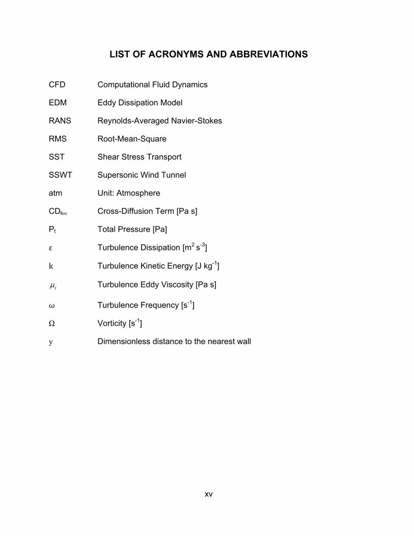
LIST OF ACRONYMS AND ABBREVIATIONS

CFD Computational Fluid Dynamics

EDM Eddy Dissipation Model

RANS Reynolds-Averaged Navier-Stokes

RMS Root-Mean-Square

SST Shear Stress Transport

SSWT Supersonic Wind Tunnel

atm Unit: Atmosphere

CDkω Cross-Diffusion Term [Pa s]

Pt Total Pressure [Pa]

ε Turbulence Dissipation [m2 s-3]

k Turbulence Kinetic Energy [J kg-1]

t Turbulence Eddy Viscosity [Pa s]

ω Turbulence Frequency [s-1]

Ω Vorticity [s-1]

y Dimensionless distance to the nearest wall

xvi


xvii

ACKNOWLEDGMENTS

I would like to extend warm appreciation in acknowledging several people whose

efforts greatly contributed to the successful completion of this thesis.

A sincere thank you to Mr. John Mobley, of the mechanical-engineering machine

shop. His dedication and precision in building the ramjet were indispensable.

Many thanks also to Mr. Douglas Seivwright, who, despite his busy schedule, took

time off to help bond the strain gauges onto the flexures, a delicate job that he has

mastered over many years.

I am grateful to Mr. John Gibson for his help in putting the ramjet together and

setting up the wind tunnel for experiments. Without his skills, the experiments would

never have run smoothly.

And finally, I thank my advisor, Professor Garth Hobson, for the opportunity to

work with him and the close guidance he provided from start to finish.

xviii


1

I. INTRODUCTION

In 1913, René Lorin, a French inventor, conceived the concept of the ramjet, a

rotor-less air-breathing jet engine. While he did not succeed in building a prototype, he

understood that there would be insufficient pressure to operate a ramjet in subsonic

flight. The interest in ramjets picked up, and in 1938, a French engineer, René Leduc,

sent the Leduc 0.10, the first ramjet-powered aircraft, into the skies. The Leduc 1.0,

achieved a Mach number of 0.85, remarkable for its time.

The capability of ramjets delivering high speed flights has always been an area of

interest to the military. In 1976, the turbo-ramjet powered SR-71, a military

reconnaissance plane made its maiden flight, achieving Mach 3.3+ with a top speed of

over 3500 m/s. While it is still the fastest manned aircraft, the bigger significance to the

military is its ability to outfly almost any threat launched against it. In 2006, the ramjet-

powered BrahMos cruise missile was introduced. At Mach 3, it is the world's fastest

cruise missile. This essentially translates to high survivability rate against any

interceptor, and hence a higher possibility of hitting the target.

While these ramjet engines powering military flight have been huge, there are

many potential uses for miniaturized ramjets in defense technologies. Possibilities

include employment as an anti-material kinetic round at standoff distances and even to

power the flight of mini/micro unmanned, aerial vehicles (UAV). However, before these

ideas turn into reality, there must be sufficient knowledge of the performance envelope

involved.

This thesis takes on the work of Fergurson [1] and Khoo [2]. In [1], a miniature

ramjet was designed for flight at Mach 4 and the cold-flow performance of the ramjet

was evaluated using Overflow computational fluid dynamics (CFD) code and partially

validated through tests in a supersonic wind tunnel (SSWT). A follow-up of the analysis

was performed in [2] with the CFD-FASTRAN code in an attempt to model the

combustion process in the ramjet. However, due to limited computing power and

limitations in the CFD code used, the analysis did not cover the operating conditions of

the ramjet.

2

In [1] and [2], the cold-flow CFD analyses showed an oblique shock forming at

the inlet cowl where a normal shock was expected. In [2], it was hypothesized that this

observation was due to the nozzle’s throat being too wide. The current research

attempts to investigate this with variations in nozzle-throat sizing.

In the design of the ramjet in [1], fuel ports were added to the nose cone of the

ramjet to induce early fuel-air mixing. However, computationally, the impact of fluid

injections through these tip ports were not analyzed. The current research aims to

determine how the flow field will be affected by fluid injection through these tip ports.

Exploiting the power of parallel processing, the present study revisits the analysis

performed in [1] and [2] using CFD code by ANSYS-CFX to perform 3-D combustion

analysis of the ramjet. Hydrogen fuel was injected through the rear fuel ports on the

struts for combustion.

Finally, in [2], the CFD predictions and experimental results in wind-tunnel testing

showed a disparity in the drag profiles observed. The present study revisits this with a

new model and sensors in a wind-tunnel experiment.

Work done in this thesis will provide a better understanding of the miniature

ramjet and lay the foundations required for a flight test.

3

II. NUMERICAL PERFORMANCE PREDICTION WITH ANSYS-CFX

A. ANSYS-CFX

In [1] and [2], the CFD codes used for the numerical performance predictions

were NASA Overflow code and the CFDRC-FASTRAN code, respectively.

For this thesis, version 14 of the ANSYS Workbench suite of tools by ANSYS,

Inc., was used. The ANSYS Workbench suite provides a simple workflow for the

management of the project, from mesh generation (ANSYS-Meshing) to problem setup,

numerical simulation, and post-processing of the simulation results.

ANSYS-CFX, a finite-volume-based CFD code by ANSYS, Inc., was used for

numerical performance predictions. ANSYS-CFX comprises CFX-PRE, CFX-SOLVER,

and CFX-POST.

In the CFD analysis with ANSYS-CFX, the meshed model was transferred into

CFX-PRE, where the problem was set up and the implicit boundary conditions were

applied. Thereafter, the CFX-SOLVER was invoked for flow computation, where the

Navier-Stokes equation was solved in its conservative form [3].

The CFX-SOLVER supports parallel processing for complex models requiring

high computational powers. Additionally, ANSYS-CFX can analyze reacting flows with

its combustion model. For this study, the eddy dissipation model (EDM) was used with

the shear stress transport (SST) turbulence model. The results of the flow computation

were then flowed to CFX-POST for viewing and post processing.

B. TURBULENCE MODELLING

At high Reynolds numbers, turbulence develops in flows; motion of the fluid

particles becomes random, with velocities and pressures varying with time [3]. For the

prediction of turbulence effects, ANYS-CFX supports numerous Reynolds-Averaged

Navier-Stokes (RANS) equation-based turbulence models. Based upon the turbulent

eddy viscosity concept, two-equation turbulence model represents the turbulence

properties of the flow with two additional transport equations. The k-epsilon (k‐ε) and k-

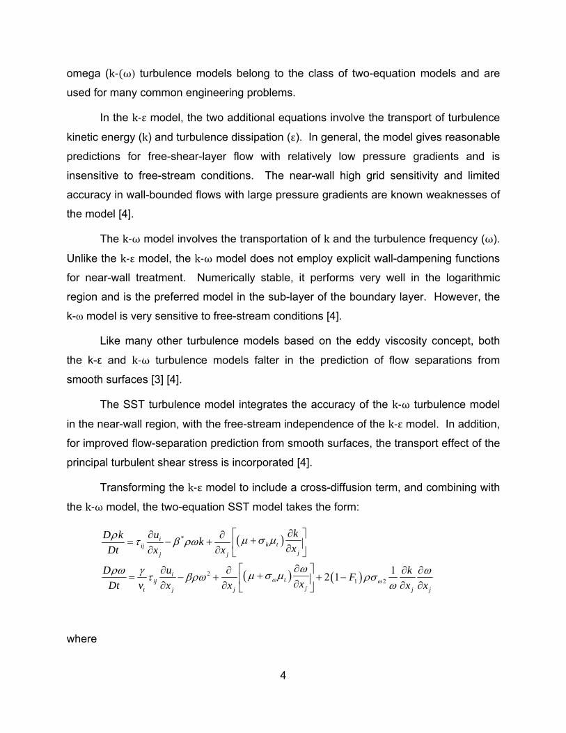
4

omega (k‐ ω) turbulence models belong to the class of two-equation models and are

used for many common engineering problems.

In the k‐ε model, the two additional equations involve the transport of turbulence

kinetic energy (k) and turbulence dissipation (ε). In general, the model gives reasonable

predictions for free-shear-layer flow with relatively low pressure gradients and is

insensitive to free-stream conditions. The near-wall high grid sensitivity and limited

accuracy in wall-bounded flows with large pressure gradients are known weaknesses of

the model [4].

The k‐ω model involves the transportation of k and the turbulence frequency (ω).

Unlike the k‐ε model, the k‐ω model does not employ explicit wall-dampening functions

for near-wall treatment. Numerically stable, it performs very well in the logarithmic

region and is the preferred model in the sub-layer of the boundary layer. However, the

k-ω model is very sensitive to free-stream conditions [4].

Like many other turbulence models based on the eddy viscosity concept, both

the k-ε and k‐ω turbulence models falter in the prediction of flow separations from

smooth surfaces [3] [4].

The SST turbulence model integrates the accuracy of the k‐ω turbulence model

in the near-wall region, with the free-stream independence of the k‐ε model. In addition,

for improved flow-separation prediction from smooth surfaces, the transport effect of the

principal turbulent shear stress is incorporated [4].

Transforming the k‐ε model to include a cross-diffusion term, and combining with

the k‐ω model, the two-equation SST model takes the form:

*

221

12 1

ik tij

jj j

itij

jt j j j j

kuD kk

xDt x x

uD kF

xDt v x x x x

where

5

2 23 3

ji kijij t ij

j i j

uu uk

x x x

The turbulent eddy viscosity is obtained from a limiter to turbulent shear stress:

1

1 2max ;t t

a kv

a F

where Ω is the absolute value of vorticity. The blending of the k‐ε and k‐ω model is

achieved through the blending functions F1 and F2, which evaluates to 1 in the near-wall

region and 0 when away from the surface.

4

21 22

2

2 2

4500tanh min max ,,0.09

2 500tanh max ,0.09

k

kk vFCD yy y

k vFy y

y is the distance to the nearest wall and CDkω is the cross-diffusion term:

202

12 ,10maxk

j j

k wCD

x x

The SST turbulence model is the default turbulence model used in this thesis.

Full derivation of the SST turbulence model is available in [5].

C. COMBUSTION MODELING

The combustion model used in the thesis is the Eddy Dissipation Model (EDM).

In the EDM, the fast chemical rate of reaction has direct relation to the molecular-level

mixing rate of the reactants. Relative to the flow transport process, the chemical

reaction rates are fast and products are formed instantaneously when mixing of the

reactants take place at the molecular level. In a turbulent flow, the eddy properties

dominate the mixing time and the molecular level mixing is defined by:

ratek

6

D. RAMJET NOMENCLATURE

For ease of reference, the various parts of the ramjet and its associated stations

are defined in Figure 1.

Figure 1. Schematic of ramjet with associated stations

0

2 3 6

7

8

961 Free Stream

7

III. COLD-FLOW CFD ANALYSIS

A. BACKGROUND AND METHODOLOGY

In [1] and [2], for efficiency, a 2-D axis-symmetrical model was used for the cold-

flow analysis of the ramjet. However, to maintain the axissymmetry, the internal struts

of the ramjet were not included in the 2-D computational model of the ramjet. In this

thesis, a more realistic 3-D computational model of the ramjet was used for the CFD

cold-flow analysis. The conditions for the simulation were set to those in the wind

tunnel for subsequent comparisons.

From [1] and [2], while a normal shock was expected to form at the inlet cowl, an

oblique shock system was instead observed. It was hypothesized that this could be due

to a non-optimized nozzle-throat diameter (too large). To investigate this, CFD

analyses were performed on the ramjet models with the nozzle-throat area of the base

model reduced by 10% to 40%, in 10% steps. The reduction of the throat areas was

aimed at increasing backpressure, thereby forcing the observed oblique shock system

into a normal shock that sits at the lip of the inlet cowl.

For the steady-state cold-flow CFD analyses, the models used were first created

in SolidWorks and then imported into ANSYS Workbench for mesh generation with the

ANSYS-Meshing utility. The meshed model then flowed into ANSYS-CFX through the

CFX-PRE – CFX-SOLVER – CFX-POST workflow previously described.

Parallel computing with over ten computers was employed to allow for faster

computation of each simulation. Typical run times of over 72 hours were experienced

on the NPS computer cluster, named “Hamming".

8

B. COMPUTATIONAL MODEL SETUP FOR COLD-FLOW ANALYSES

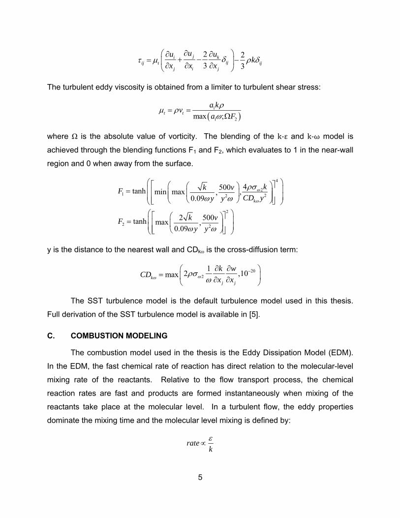
1. Three-Dimensional Computational Model

Exploiting the two axes of symmetry (Figure 2), the computational domain of the

ramjet was modeled to consist of a “quarter-cut” of the ramjet in a block of fluid (Figure

3). Similar to [1] and [2], to simplify the computation for the cold-flow analysis, the fuel-

injection ports on the ramjet were not modeled.

Figure 2. Geometry of ramjet with two axes of symmetry

Figure 3. Three-dimensional computational model for cold-flow analysis, with boundary namespace

Side View Front View

Rectangular Control Volume (Fluid)

Axes of Symmetry

Ramjet


Isometric View

Inlet Outlet

Top

Ramjet Symmetry Planes

9

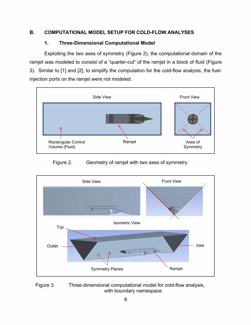
The 3-D grid of the computational model was generated with the ANSYS

meshing utility. For the default model, a total of 2.69 million nodes and 14.99 million

elements was generated. Figure 4 presents the mesh profile of the computational model,

with a close-up view of the meshes at the inlet cowl, showing the inflation layers at the

surface. Details of the meshing parameters can be found in Appendix A.

Figure 4. Mesh of computation model for cold-flow analysis

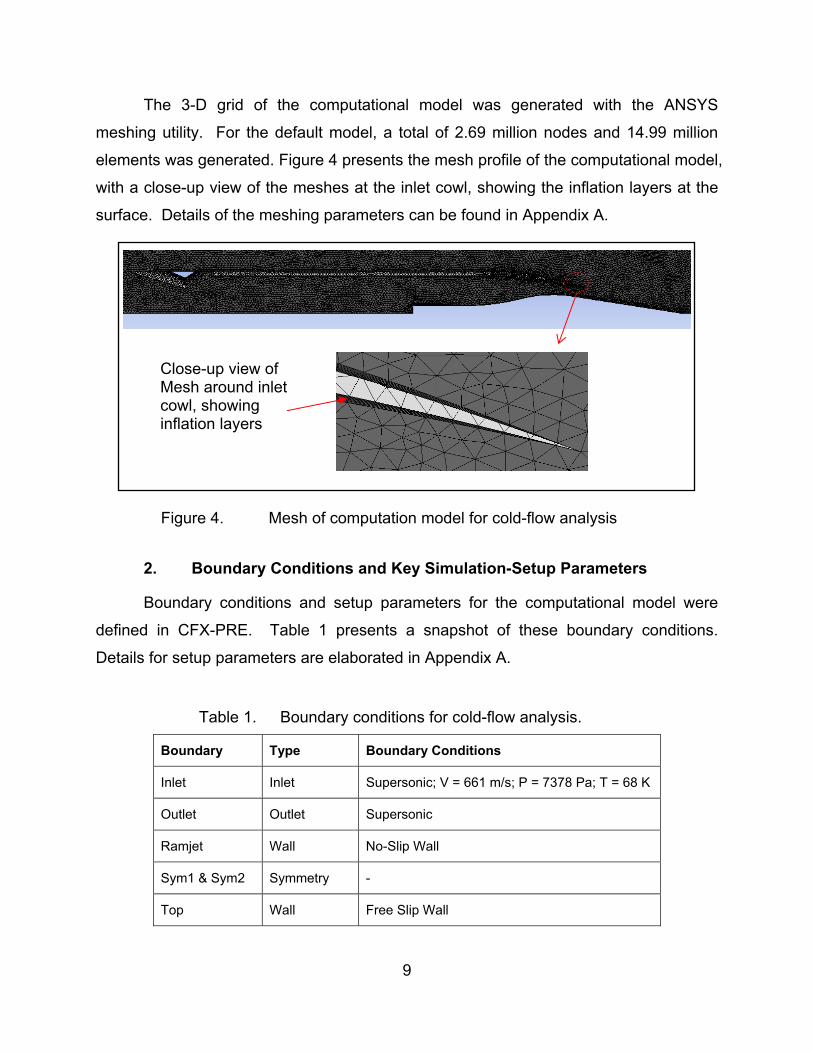
2. Boundary Conditions and Key Simulation-Setup Parameters

Boundary conditions and setup parameters for the computational model were

defined in CFX-PRE. Table 1 presents a snapshot of these boundary conditions.

Details for setup parameters are elaborated in Appendix A.

Table 1. Boundary conditions for cold-flow analysis.

Boundary Type Boundary Conditions

Inlet Inlet Supersonic; V = 661 m/s; P = 7378 Pa; T = 68 K

Outlet Outlet Supersonic

Ramjet Wall No-Slip Wall

Sym1 & Sym2 Symmetry -

Top Wall Free Slip Wall

Close-up view of Mesh around inlet cowl, showing inflation layers

10

Table 2 provides a list of important parameters that must be set in CFX-PRE.

Table 2. Important setup parameters for CFX-PRE.

Parameter Location Description

High Speed Numerics

Solver Control Advance Options Compressibility Control

For better resolution of high-speed flows and shocks.

Max Continuity Loop

Expert Parameters Convergence Control

Set to 3. Necessary for high-speed flows to aid convergence

C. RESULTS AND DISCUSSION

1. Flow-Profile Comparison

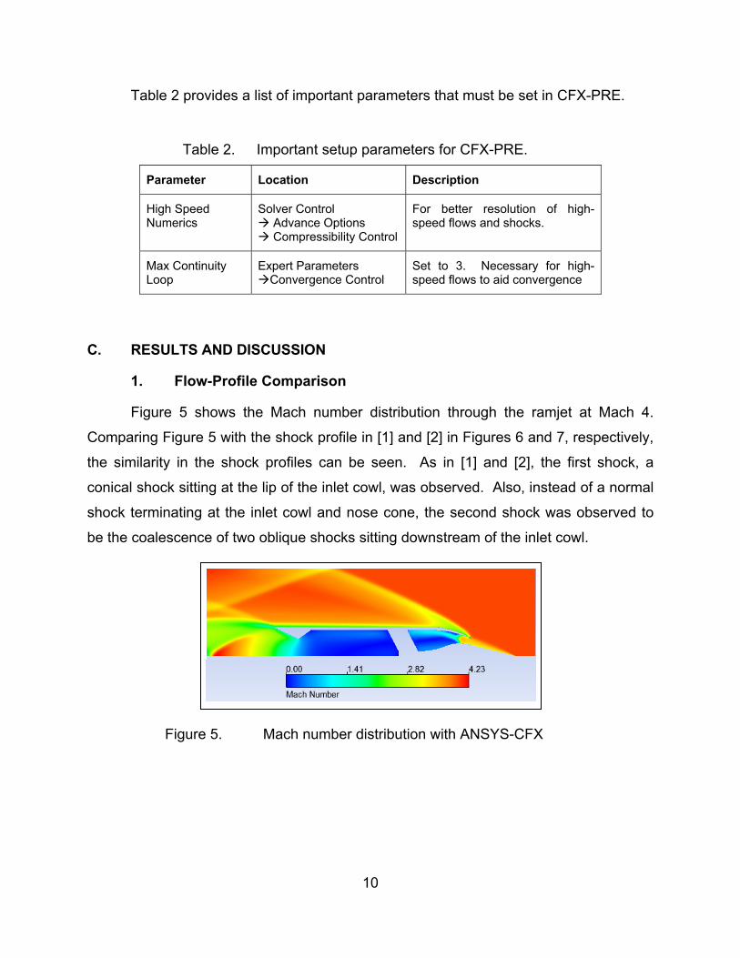
Figure 5 shows the Mach number distribution through the ramjet at Mach 4.

Comparing Figure 5 with the shock profile in [1] and [2] in Figures 6 and 7, respectively,

the similarity in the shock profiles can be seen. As in [1] and [2], the first shock, a

conical shock sitting at the lip of the inlet cowl, was observed. Also, instead of a normal

shock terminating at the inlet cowl and nose cone, the second shock was observed to

be the coalescence of two oblique shocks sitting downstream of the inlet cowl.

Figure 5. Mach number distribution with ANSYS-CFX

11

Figure 6. Mach number distribution with Overflow code [1]

Figure 7. Mach number distribution with CFDRC-FASTRAN [2]

The density, pressure, and temperature distributions are shown in Figures 8 to

10, respectively. Comparing these with those in [1] and [2], a great level of congruency

between the plots was also observed.

Figure 8. Pressure distribution with ANSYS-CFX

12

Figure 9. Density distribution with ANSYS-CFX

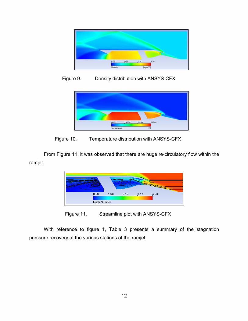
Figure 10. Temperature distribution with ANSYS-CFX

From Figure 11, it was observed that there are huge re-circulatory flow within the

ramjet.

Figure 11. Streamline plot with ANSYS-CFX

With reference to figure 1, Table 3 presents a summary of the stagnation

pressure recovery at the various stations of the ramjet.

13

Table 3. Summary of stagnation pressure recovery at various stations

Free Stream Stagnation Pressure (Pt∞) 1,116.36 kPa

Station

Number

(n)

Theoretical Stagnation

Pressure Recovery Ratio

(P'tn/P t∞) from [1]

Stagnation

Pressure

(Ptn)

Stagnation

Pressure Recovery

Ratio (Ptn/P t∞)

2 0.991 980.54 kPa 0.878

3 0.676 219.68 kPa 0.197

61 - 126.64 kPa 0.113

7 - 119.72 kPa 0.107

From Table 3, the stagnation pressure recovery ratios obtained from the CFD

showed that the current ramjet design provides for poor pressure recovery. The biggest

drop in pressure recovery ratio occurred at station 3 - after the second shock system.

This indicated that the subsonic diffuser system of the inlet would need to be

redesigned to improve the stagnation pressure recovery.

The drag on the ramjet was computed to be 26.838N, with a corresponding drag

coefficient of 0.371. This compares favorably with the drag of 21.35 N computed in [1].

14

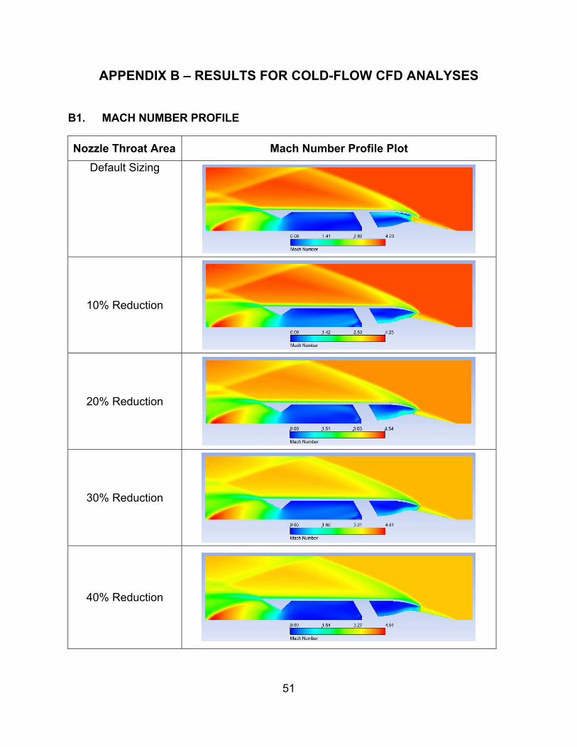
2. Results of Cold-Flow Analysis with Varied Nozzle-Throat Area

Figures 12 to 15 shows the Mach-number profile achieved with the

corresponding reduced nozzle-throat area. Figure 16 shows the shock indicator plot for

the reduced nozzle-throat areas.

Figure 12. Cold-flow shock profile with 10% reduction in nozzle-throat area



15


Figure 16. Shock indicator around inlet for a) 10% b) 20%, c) 30%, d) 30% reduction in throat area

As seen in figures 15, 16 and Table 3, reducing the nozzle-throat area resulted in

increased back pressure which pushed the coalesced oblique shocks upstream towards

the inlet cowl.

a. At 10% and 20% reduction in nozzle-throat area, the two coalesced

oblique shocks remained downstream the lip of the inlet cowl.

b) - 20% Throat Area

c) - 30% Throat Area d) - 40% Throat Area

a) - 10% Throat Area

16

b. At 30% reduction in nozzle-throat area, a normal shock was formed

at the lip of the inlet cowl. However, as shown in figures 15 and 16b, unlike theoretical

predictions, this normal shock is not truly orthogonal to the flow.

c. At 40% reduction in nozzle-throat area, the coalesced oblique

shocks were pushed into a normal shock which developed upstream the lip of the inlet

cowl, resulting in flow spillage.

While the results showed that a reduction of 30% in the nozzle-throat area would

site the normal shock at the lip of the inlet cowl, in reality, this may not be desirable.

With the normal shock sitting on the lip of the inlet cowl, slight perturbations in the

chamber conditions can push the normal shock upstream, causing the inlet to unstart.

Hence, depending on the required performance buffer, the nozzle should be sized

accordingly to site the shock at the desired position.

17

IV. CFD ANALYSIS FOR AIR INJECTION THROUGH THE TIP PORTS


In [1], from the SSWT experiment, it was reported that atmospheric air from

outside the SSWT was seeping into the ramjet model through the open ports, resulting

in the air ejecting from the tip ports of the ramjet’s nose cone. It was suspected that this

ejected air interacted wih the downstream shock structure.

To investigate the effect of this interaction, CFD analyses for injection of air

through the tip ports were performed with total pressure settings of 1 atmosphere, 0.75

atmosphere and 0.5 atmosphere. The other boundary conditions were selected such

that they replicate the SSWT experiment conditions. This allowed the results to be

compared to the CFD cold-flow analysis results and will facilitate the conduct of any

subsequent verification in the SSWT.

Parallel computing over four local processors was employed to allow for faster

computation of each simulation. Typical run times of 7 to 8 hours were experienced.

B. COMPUTATIONAL MODEL SETUP

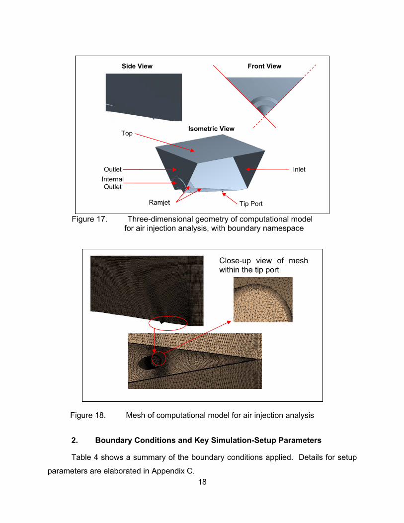
1. Three-Dimensional Model Setup

The 3-D computational model (Figure 17) used for the steady-state injection

analysis was a quarter-cut model of the ramjet’s nose cone.

The 3-D mesh of the computational model was generated with the ANSYS

meshing utility. A total of 456k nodes and 2.17 million elements was generated. Figure

18 displays the mesh profile for the computational model, with a close-up view of the

meshes at the tip ports of the ramjet’s nose cone. The meshing parameters are

detailed in Appendix C.

18

Figure 17. Three-dimensional geometry of computational model for air injection analysis, with boundary namespace

Figure 18. Mesh of computational model for air injection analysis


Table 4 shows a summary of the boundary conditions applied. Details for setup

parameters are elaborated in Appendix C.

Close-up view of mesh within the tip port

Front View Side View

Isometric View

Outlet

Top

Inlet

Ramjet Tip Port

Internal Outlet

19

Table 4. Boundary conditions for air injection analysis


Inlet Inlet Supersonic; V = 661 m/s; P = 7378 Pa; T = 68 K


Internal Outlet Outlet Supersonic1


Tip Ports Inlet Subsonic; Total Pressure = 101325 Pa; T = 298.15 K

Top Wall Free-Slip Wall



Detailed results for the tip port air injection analysis can found in Appendix D.

Figure 19 to 21 shows the Mach number distribution for the air injection at total pressure

settings of 0.5 atm, 0.75 atm and 1 atm. From these figures, it is apparent that the

injected air perturbed the conical shock, deflecting the conical shock away from the

nose cone.

Figure 19. Mach number distribution for air injection through tip port with Pt = 0.5 atm

1 The supersonic boundary condition for the "Internal Outlet" was determined from the default cold-

flow solution.

20

Figure 20. Mach number distribution for air injection through tip port with Pt = 0.75 atm

Figure 21. Mach number distribution for air injection through tip port with Pt = 1 atm

Upstream of the tip port, where the conical shock remained unperturbed, the

Mach number at the fringe was computed to be 3.65. If unperturbed, this will be the

Mach number for the conical shock incident on the lip of the ramjet’s inlet cowl.

21

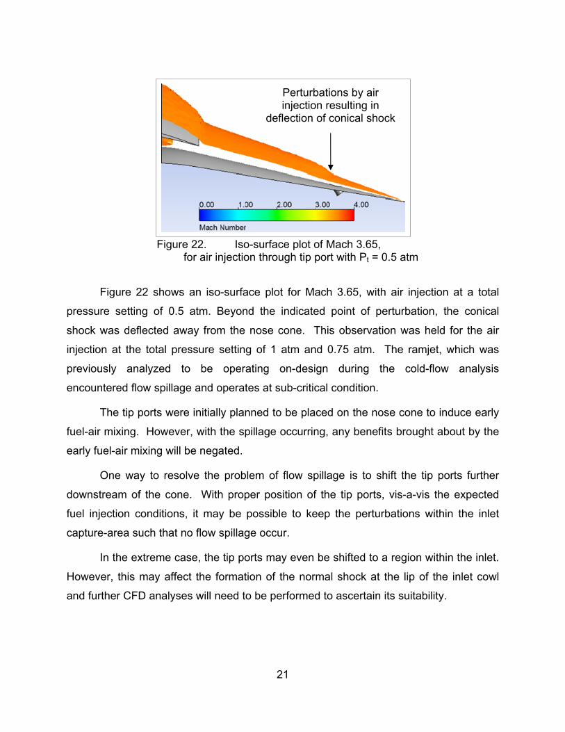
Figure 22. Iso-surface plot of Mach 3.65, for air injection through tip port with Pt = 0.5 atm

Figure 22 shows an iso-surface plot for Mach 3.65, with air injection at a total

pressure setting of 0.5 atm. Beyond the indicated point of perturbation, the conical

shock was deflected away from the nose cone. This observation was held for the air

injection at the total pressure setting of 1 atm and 0.75 atm. The ramjet, which was

previously analyzed to be operating on-design during the cold-flow analysis

encountered flow spillage and operates at sub-critical condition.

The tip ports were initially planned to be placed on the nose cone to induce early

fuel-air mixing. However, with the spillage occurring, any benefits brought about by the

early fuel-air mixing will be negated.

One way to resolve the problem of flow spillage is to shift the tip ports further

downstream of the cone. With proper position of the tip ports, vis-a-vis the expected

fuel injection conditions, it may be possible to keep the perturbations within the inlet

capture-area such that no flow spillage occur.

In the extreme case, the tip ports may even be shifted to a region within the inlet.

However, this may affect the formation of the normal shock at the lip of the inlet cowl

and further CFD analyses will need to be performed to ascertain its suitability.

Perturbations by air injection resulting in

deflection of conical shock

22


23

V. COMBUSTION CFD ANALYSIS


In [2], a mixture analysis of propane and air was performed on a 45-degree slice

of the ramjet. However, due to the limitations in computing resources and the CFD code

used, the combustion CFD analysis was performed on a 2-D computational model, with

propane injected into the ramjet at low speeds.

In this thesis, a 3-D computational model was used for the steady-state

combustion analysis in ANSYS-CFX. The combustion analysis was based upon a

single-step hydrogen–oxygen (H2–O2) combustion model within air and with the “eddy

dissipation combustion model”.

The stoichiometric combustion of hydrogen and air (with 23.3% oxygen) requires

a hydrogen-air mass ratio of 1:30.94. With the ramjet operating at designed condition,

the required mass-flow rate of the hydrogen fuel was calculated to be 4.07 x 10-4 kg/s

(Appendix E) and this equated to an injection velocity of more than 1000 m/s.

With the high fuel injection velocity required, any combustion that developed will

be highly unsteady may be blown out of the nozzle. With this consideration, a moderate

approach was taken for the combustion analysis with fuel injection at 400m/s.

B. COMPUTATIONAL MODEL SETUP FOR MIXING-FLOW ANALYSIS

1. Three-Dimensional Model Setup

The 3-D computational model (Figure 23) used for the combustion analysis is a

quarter-cut model of the ramjet. For simplicity in flow computation, only the rear fuel-

injection ports on the struts were modeled. Since the interest in the combustion

analysis is confined to the internal flow, to reduce the complexity and time required for

simulation, irrelevant external-flow regions were excluded from the computational model.

24

Figure 23. Three-dimensional geometry of computational model for combustion analysis, with boundary namespace

The 3-D mesh of the computational model was generated with the ANSYS

meshing utility. A total of 1.82 million nodes and 6.57 million elements was generated.

Figure 24 displays the mesh profile for the computational model, with a close-up view of

the meshes at the rear fuel ports showing the inflation layers. The meshing parameters

are detailed in Appendix F.

Figure 24. Mesh of computational model for mixing analysis


Isometric View

Inlet

Outlet

Rear Injection Ports

Ramjet Symmetry Planes

Opening

Close-up view of mesh within one of the fuel ports

25


Table 5 shows a summary of the boundary conditions applied. Details for the

setup parameters are elaborated in Appendix F.

Table 5. Boundary conditions for mixing analysis


Inlet Inlet Supersonic; V = 1180.17 m/s; P = 7504.8 Pa; T = 216.65 K



Rear Ports Inlet Subsonic; V = 50 m/s2; Total Temperature = 300 K

Opening Opening Subsonic; P = 7504.8 Pa; T = 216.65 K


In ANSYS-CFX, for combustion to take place, it is necessary for the

computational domain to contain a small fraction of the products. Hence, a 1% mass

fraction of H2O was set in the computational domain.

Due to the complex flow model, a solution with no combustion was first obtained.

This pre-combustion solution was then used as the input for the actual combustion

analysis.


Figure 25 shows the RMS convergence history of the simulation run with the

reference time step labeled.

2 Injection velocity for hydrogen was ramped up gradually from 50 m/s to the required velocity of 400

m/s.

26

Figure 25. RMS convergence history with reference time step for hydrogen injection

Prior to and inclusive of reference time step 1, no combustion was simulated.

After reference time step 1, combustion was activated. Beyond reference time step 3,

the solution diverged and the simulation terminated prematurely.

Figures 25 shows the temperature distribution of the computational model, at the

referenced time step.

27

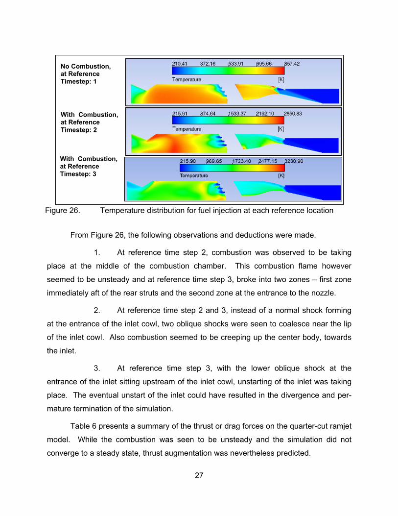
Figure 26. Temperature distribution for fuel injection at each reference location

From Figure 26, the following observations and deductions were made.

1. At reference time step 2, combustion was observed to be taking

place at the middle of the combustion chamber. This combustion flame however

seemed to be unsteady and at reference time step 3, broke into two zones – first zone

immediately aft of the rear struts and the second zone at the entrance to the nozzle.

2. At reference time step 2 and 3, instead of a normal shock forming

at the entrance of the inlet cowl, two oblique shocks were seen to coalesce near the lip

of the inlet cowl. Also combustion seemed to be creeping up the center body, towards

the inlet.

3. At reference time step 3, with the lower oblique shock at the

entrance of the inlet sitting upstream of the inlet cowl, unstarting of the inlet was taking

place. The eventual unstart of the inlet could have resulted in the divergence and per-

mature termination of the simulation.

Table 6 presents a summary of the thrust or drag forces on the quarter-cut ramjet

model. While the combustion was seen to be unsteady and the simulation did not

converge to a steady state, thrust augmentation was nevertheless predicted.

No Combustion, at Reference Timestep: 1

With Combustion, at Reference Timestep: 2

With Combustion, at Reference Timestep: 3

28

Table 6. Summary of thrust and drag forces on ramjet for combustion analyses

Fuel Injection Velocity Analysis Type

(Reference Time Step)

Thrust / Drag Forces

400 m/s No Combustion (1) Drag: 3.304 N

Combustion (2) Thrust: 1.379 N

Combustion (3) Thrust: 2.253 N

From the results, before proceeding further, it is recommended that the problem

of the unstable combustion be resolved first. With the fuel injection velocity at 400m/s,

this may still be too fast for the combustion to develop properly. Reducing the fuel

injection velocity will allow more time for the fuel-air mixing to take place, thereby

allowing the combustion to develop properly. To reduce the fuel injection velocity, the

current fuel injection ports may be widened and more fuel injection ports may be added

to the struts and the center body. In addition, flame holders may be introduced into the

ramjet, aft of the struts to stabilize the flame.

29

V. SUPERSONIC WIND-TUNNEL EXPERIMENT AND COMPARISON WITH CFD


The SSWT experiment was first ran in [1] and due to the imperfections of the

physical ramjet model, the schlieren image showed a lopsided conical shock angle

attached to the tip of the nose cone.

With the NASA Overflow code, the drag on the ramjet was predicted in [1] to be

21.351 N. In [2], based on a 2-D double wedge profile, the drag on each load flexure

was calculated to be 20.177N. Overall, the drag for the ramjet model in the SSWT was

predicted to be 61.71N. Wind tunnel tests however, showed the drag to be 57.85N (13

lbf). The over-prediction in drag was previously hypothesized to be the result of using a

simple 2-D model for the load flexure, which did not account for sweep effects that

would reduce the load prediction.

The temperature of the test section in the SSWT while running is 68K, and the

strain gauges used in [2] were operating outside their performance envelope. It was

believed that these were more likely to cause the observed disparity in drag

measurement and prediction.

Figure 27 shows a top-down schematic of the ramjet mounted within the SSWT.

With the air on in the wind tunnel, the drag induced on the ramjet and inner flexure will

cause axial deflection of the flexure beams, changing the resistance of the strain

gauges. Measuring the voltage difference from this change allows the determination of

the drag induced on the ramjet and inner flexures.

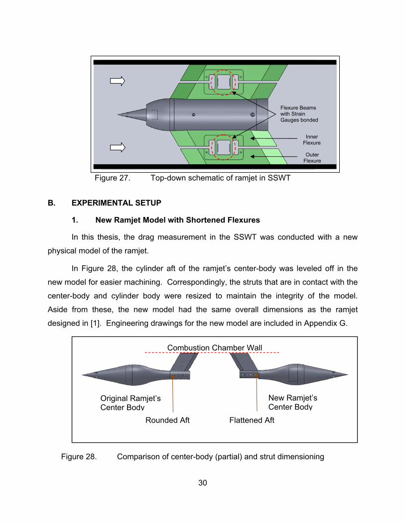
30

Figure 27. Top-down schematic of ramjet in SSWT

B. EXPERIMENTAL SETUP

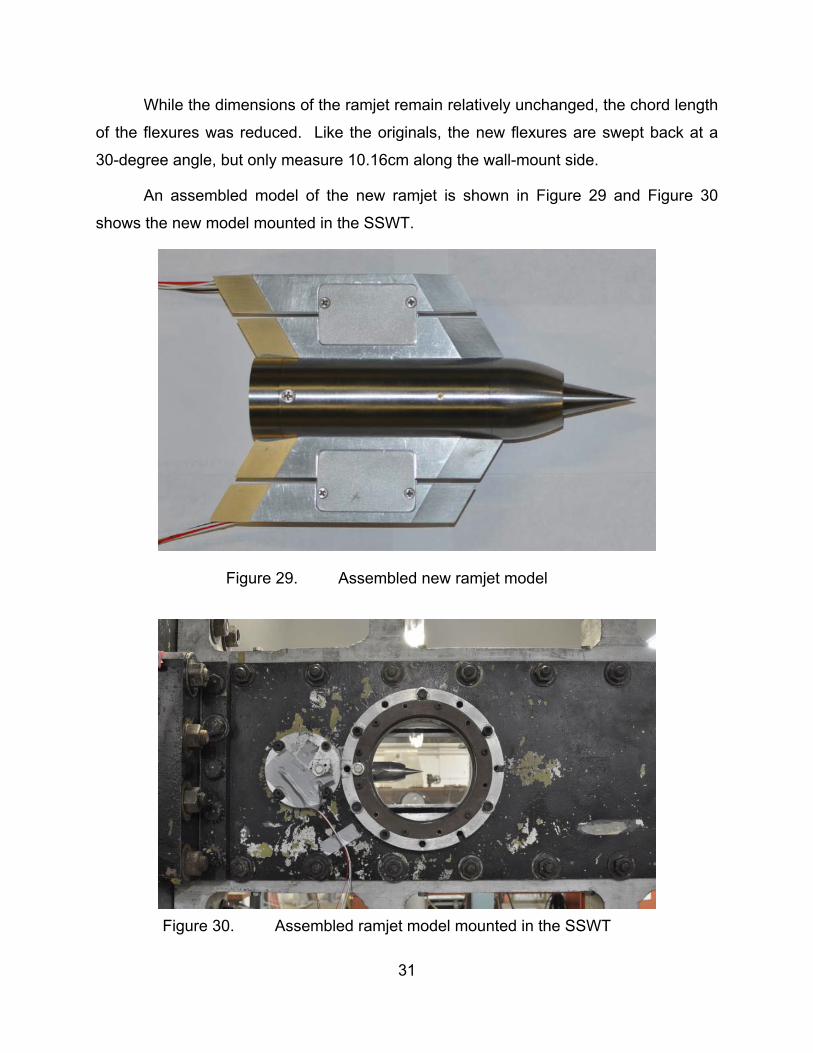
1. New Ramjet Model with Shortened Flexures

In this thesis, the drag measurement in the SSWT was conducted with a new

physical model of the ramjet.

In Figure 28, the cylinder aft of the ramjet’s center-body was leveled off in the

new model for easier machining. Correspondingly, the struts that are in contact with the

center-body and cylinder body were resized to maintain the integrity of the model.

Aside from these, the new model had the same overall dimensions as the ramjet

designed in [1]. Engineering drawings for the new model are included in Appendix G.

Figure 28. Comparison of center-body (partial) and strut dimensioning

Fre

e S

trea

m c

ondi

tions

at

M=

4

Outer Flexure

Inner Flexure

Flexure Beams with Strain Gauges bonded

Original Ramjet’s Center Body

New Ramjet’s Center Body

Rounded Aft Flattened Aft

Combustion Chamber Wall

31

While the dimensions of the ramjet remain relatively unchanged, the chord length

of the flexures was reduced. Like the originals, the new flexures are swept back at a

30-degree angle, but only measure 10.16cm along the wall-mount side.

An assembled model of the new ramjet is shown in Figure 29 and Figure 30

shows the new model mounted in the SSWT.

Figure 29. Assembled new ramjet model

Figure 30. Assembled ramjet model mounted in the SSWT

32

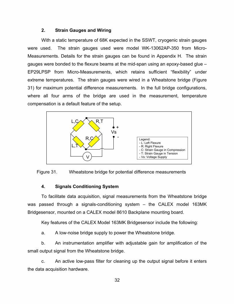
2. Strain Gauges and Wiring

With a static temperature of 68K expected in the SSWT, cryogenic strain gauges

were used. The strain gauges used were model WK-13062AP-350 from Micro-

Measurements. Details for the strain gauges can be found in Appendix H. The strain

gauges were bonded to the flexure beams at the mid-span using an epoxy-based glue –

EP29LPSP from Micro-Measurements, which retains sufficient “flexibility” under

extreme temperatures. The strain gauges were wired in a Wheatstone bridge (Figure

31) for maximum potential difference measurements. In the full bridge configurations,

where all four arms of the bridge are used in the measurement, temperature

compensation is a default feature of the setup.

Figure 31. Wheatstone bridge for potential difference measurements

4. Signals Conditioning System

To facilitate data acquisition, signal measurements from the Wheatstone bridge

was passed through a signals-conditioning system – the CALEX model 163MK

Bridgesensor, mounted on a CALEX model 8610 Backplane mounting board.

Key features of the CALEX Model 163MK Bridgesensor include the following:

a. A low-noise bridge supply to power the Wheatstone bridge.

b. An instrumentation amplifier with adjustable gain for amplification of the

small output signal from the Wheatstone bridge.

c. An active low-pass filter for cleaning up the output signal before it enters

the data acquisition hardware.

Legend: - L: Left Flexure - R: Right Flexure - C: Strain Gauge in Compression - T: Strain Gauge in Tension - Vs: Voltage Supply

L,C

L,T

R,C

R,T +

-

V

Vs

33

The CALEX Model 8610 Backplane supports the mounting of up to eight signals-

conditioning cards. Figure 32 shows the Bridgesensor mounted on the CALEX Model

8610 Backplane.

Figure 32. Signals-conditioning system

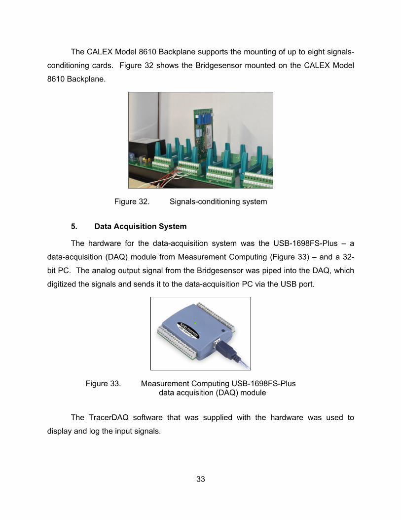
5. Data Acquisition System

The hardware for the data-acquisition system was the USB-1698FS-Plus – a

data-acquisition (DAQ) module from Measurement Computing (Figure 33) – and a 32-

bit PC. The analog output signal from the Bridgesensor was piped into the DAQ, which

digitized the signals and sends it to the data-acquisition PC via the USB port.

Figure 33. Measurement Computing USB-1698FS-Plus data acquisition (DAQ) module

The TracerDAQ software that was supplied with the hardware was used to

display and log the input signals.

34

C. PROCEDURES

The following procedures were performed sequentially. The details for these

procedures are presented in Appendix I.

1. Calibration of the signal conditioning system to obtain the correct input-to-

output response required.

2. Calibration of the flexure arms to determine the expected range of output

response.

3. SSWT experiment to measure the drag induced on the ramjet and flexures

using the collected output signal response.

D. CFD DRAG PREDICTION

For CFD drag prediction, an equivalent of the experimental ramjet model is

shown in Figure 34.

Physically, adding the pair of flexures onto the ramjet breaks the two-plane

symmetrical model into a single-plane symmetrical model. In the drag-prediction model,

the computational model still assumes a two-plane symmetrical model. The ramjet and

the flexure, however, were defined as separate entities so that the drag on the ramjet

and flexures can be obtained separately. The final drag for the ramjet and flexures will

be four times and twice the drag computed in ANSYS-CFX, respectively. Details for

setting up the computational domain for CFD drag prediction are shown in Appendix J.

35

Figure 34. 3-D computational model for cold-flow drag analysis, with boundary namespace

Figure 35 shows a comparison of the physical and computational model of the

flexure used. In the SSWT experiment, drag is determined from the deflections of the

flexure beams, and the outer flexure is merely an extension of the wall to attach the

flexure beams to the inner flexure. Unlike the experiment requirements, we do not need

the flexure beams for drag calculations in CFD. Hence, the simplified and equivalent

model of the inner flexure shown in Figure 35b was used.

Figure 35. Comparison of (a) Physical flexure model and (b) Equivalent CFD flexure model


Isometric View

Inlet Outlet

Top

Ramjet Symmetry Planes Flexure

Inner Flexure (Ramjet Side)

Outer Flexure (Wall Side)

(a) (b)

36

E. RESULTS AND DISCUSSION

1. SSWT Experiment

Two runs were conducted in the SSWT. A representative schlieren image for the

experiments is shown in Figure 36. With the ramjet mounted at zero angle of attack, the

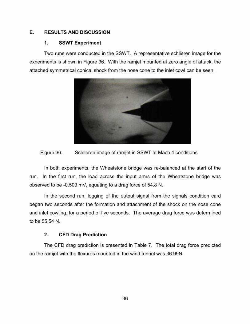
attached symmetrical conical shock from the nose cone to the inlet cowl can be seen.

Figure 36. Schlieren image of ramjet in SSWT at Mach 4 conditions

In both experiments, the Wheatstone bridge was re-balanced at the start of the

run. In the first run, the load across the input arms of the Wheatstone bridge was

observed to be -0.503 mV, equating to a drag force of 54.8 N.

In the second run, logging of the output signal from the signals condition card

began two seconds after the formation and attachment of the shock on the nose cone

and inlet cowling, for a period of five seconds. The average drag force was determined

to be 55.54 N.

2. CFD Drag Prediction

The CFD drag prediction is presented in Table 7. The total drag force predicted

on the ramjet with the flexures mounted in the wind tunnel was 36.99N.

37

Table 7. CFD drag prediction

Predicted Drag Remarks

Ramjet 26.67 N -

Flexure 5.16 N For each Flexure

Total 36.99 N -

3. Discussion

A summary of the various CFD predicted results and SSWT result is presented in

Table 8.

Table 8. Summary of predicted and measured drag forces

Parts Ramjet Flexures Total Remarks

Predicted in

ANSYS CFX

26.67 N 10.32 N 36.99 N -

Predicted in [1] 21.35 N - 61.71 N

Combined

prediction Predicted in [2] - 40.36 N

Current

Experimental

Results

- - 55.17 N -

Experimental

Results in [2]

- - 57.83 N -

While the experimental drag forces were seen to be very similar, the CFD drag

force prediction by ANYS CFX was very different from that predicted by [2]. ANSYS

CFX predicted a very low drag for the flexures.

38

With the large difference in drag predicted in ANSYS-CFX, a check was

performed on the drag predictions. The drag force induced on a body is correlated to

the "obstruction" seen by the flow. The ratios of the cross-section projected frontal area

of the ramjet and flexures seen by the flow and the ANSYS-CFX predicted drag forces

were computed to be 2.56:1 and 2.58:1, indicating that the results from ANSYS-CFX

may not be erroneous.

With the two experimental results agreeing, there is no reason to suspect the

results. However, in the conduct of the experiment, the following observations and

recommendations are made for better experimental accuracies.

1. While the model fitted into the test section, when the windows were

closed, the bridge was unbalanced, indicating an inward compressing force on the

model. While these were subsequently neutralized before the run, this compressing

force may affect the axially measured drag force. The flexures should be redesigned to

reduce the impact of any compressive or tensile forces acting on the ramjet body, as

this could affect the drag measurements.

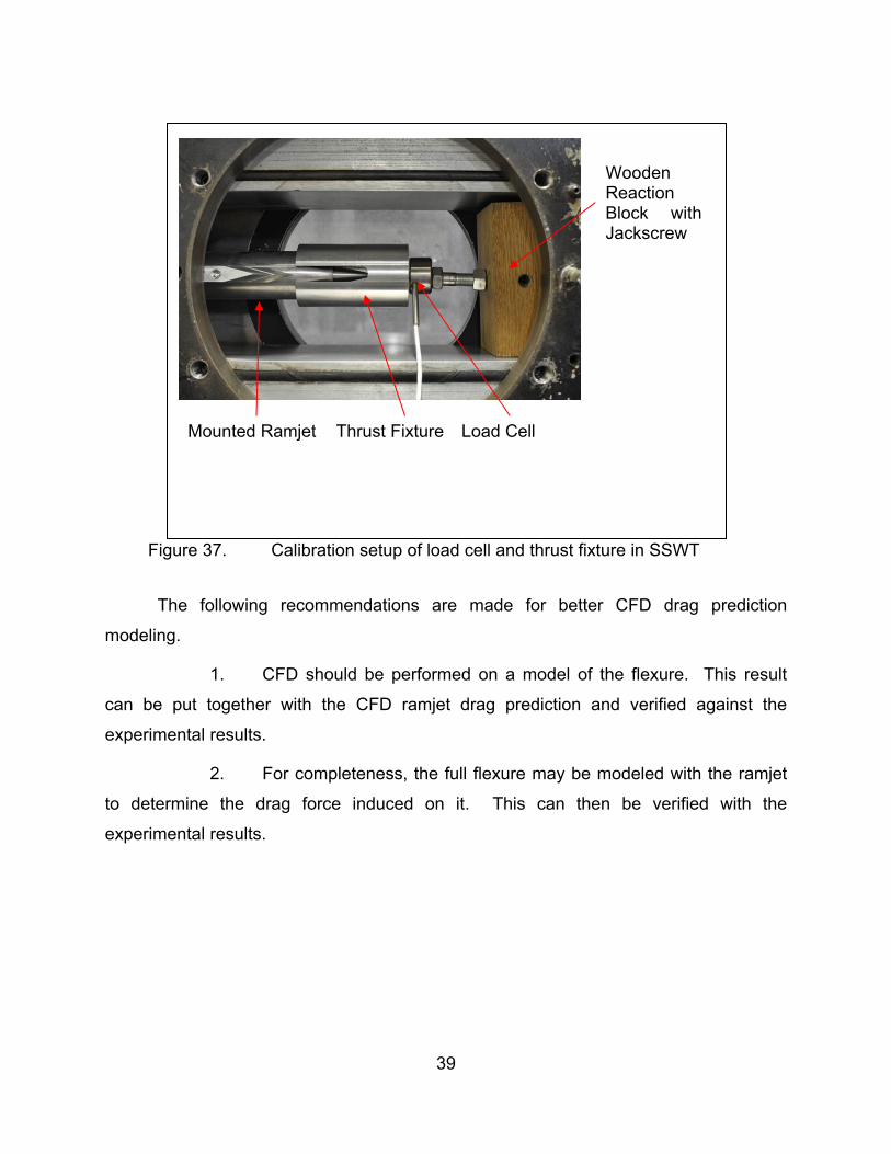
2. Figure 37 shows the setup for strain gauge calibration. The

jackscrew was tightened to vary the applied force on the ramjet and the potential

difference is measured across the Wheatstone bridge. Despite measurements taken to

ensure that the load cell was properly wedged between the jackscrew and the thrust

fixture, the applied load could not be stabilized. It is suspected that this was due to the

creep of the wooden reaction block and the thrust fixture. Eventually, over a hundred

readings at varying loads were taken to averaged out the potential errors from the

measurements. To reduce errors in calibration due to the creep, the thrust fixture

should be lengthened such that it rests on the inner flexures instead of the diffuser.

39

Figure 37. Calibration setup of load cell and thrust fixture in SSWT

The following recommendations are made for better CFD drag prediction

modeling.

1. CFD should be performed on a model of the flexure. This result

can be put together with the CFD ramjet drag prediction and verified against the

experimental results.

2. For completeness, the full flexure may be modeled with the ramjet

to determine the drag force induced on it. This can then be verified with the

experimental results.

Mounted Ramjet Thrust Fixture Load Cell

Wooden Reaction Block with Jackscrew

40


41

VII. CONCLUSIONS AND RECOMMENDATIONS

A successful cold-flow model was developed in ANSYS-CFX. On the current

ramjet design, the diffuser of the inlet would need to be redesigned to improve its total

pressure recovery. This model can be used as a baseline model for comparison with

subsequent CFD analysis.

The effects of fluid injection through the existing tip ports were investigated. It

was determined that fluid injection through the current tip ports at total pressure settings

of 0.5 atm and higher would perturb the conical shock, resulting in flow spillage at the

inlet region.

An initial combustion model was developed in ANSYS-CFX using hydrogen gas

injected aft of the struts. Results suggest that fuel combustion with the current design

would result in thrust augmentation. However, for combustion and thrust to be

sustained, the model will need to be modified. Computationally, with further

improvement, it is likely that a suitable combustion model can be developed.

A SSWT experimentation was performed, and the measured drag force of

55.17N was within 5% of the drag measurements in [2]. The current CFD model was

determined to under predict the drag force induced on the ramjet and flexures.

Results from the CFD analysis showed the flow field to be very complex. As

such, a mesh-sensitivity study should be performed to determine the sufficiency of the

current mesh resolution in capturing the complex flow field.

42


43

APPENDIX A – DETAIL SETUP FOR COLD-FLOW ANALYSIS

A1. MESH SETUP

Table 9. Details of mesh setup for cold-flow analysis

Defaults

Physics Preference CFD

Solver Preference CFX

Relevance 50

Sizing

Use Advance Size Function On: Proximity and Curvature Relevance Centre Fine Initial Size Seed Active Assembly Smoothing High

Transition Slow Span Angle Centre Fine

‐ Curvature Normal Angle 15 deg

‐ Proximity Accuracy 0.6

‐ Num Cells Across Gap Default (3)

‐ Min Size 0.0001 m

‐ Proximity Min Size 0.0001 m

‐ Max Face Size 0.0008 m ‐ Max Size 0.0008 m

‐ Growth Rate 1.1

Inflation

Use Automatic Inflation None

Patch Conforming Option

Triangle Surface Mesher Program Controlled

Advance

Shape Checking CFD Element Midside Nodes Dropped Extra Retries for Assembly Yes

Mesh Morphing Disabled

44

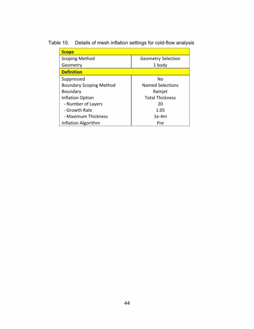
Table 10. Details of mesh inflation settings for cold-flow analysis

Scope

Scoping Method Geometry Selection

Geometry 1 body

Definition

Suppressed No Boundary Scoping Method Named Selections Boundary Ramjet Inflation Option Total Thickness ‐ Number of Layers 20 ‐ Growth Rate 1.05

‐ Maximum Thickness 1e‐4m

Inflation Algorithm Pre

45

A2. CFX-PRE SETUP PARAMETERS

Table 11. Default domain for cold-analysis

BASIC SETTINGS

Location and Type

‐ Location <use default>

‐ Domain Type Fluid Domain

‐ Coordinate Frame Coord 0

Fluid and Particles Definition for Fluid 1 ‐ Option: Material Library ‐ Material Air Ideal Gas

‐ Morphology Continuous Fluid

Domain Models

‐ Pressure Reference Pressure 0 Pa ‐ Buoyancy Model Option Non‐Buoyant ‐ Domain Motion Option Stationary

‐ Mesh Deformation Option None

FLUID MODELS

Heat Transfer Option Total Energy

Turbulence

‐ Option Shear Stress Transport

‐ Transitional Turbulence Gamma Theta Model

Combustion Option None

Thermal Radiation Option None

46

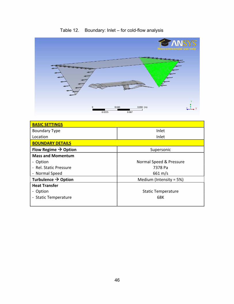
Table 12. Boundary: Inlet – for cold-flow analysis

BASIC SETTINGS

Boundary Type Inlet

Location Inlet

BOUNDARY DETAILS

Flow Regime Option Supersonic

Mass and Momentum

‐ Option Normal Speed & Pressure ‐ Rel. Static Pressure 7378 Pa ‐ Normal Speed 661 m/s

Turbulence Option Medium (Intensity = 5%)

Heat Transfer ‐ Option Static Temperature

‐ Static Temperature 68K

47

Table 13. Boundary: Outlet – for cold-flow analysis

BASIC SETTINGS

Boundary Type Outlet

Location Outlet

BOUNDARY DETAILS


Table 14. Boundary: Sym1 – for cold-flow analysis

BASIC SETTINGS

Boundary Type Symmetry

Location Sym1

48

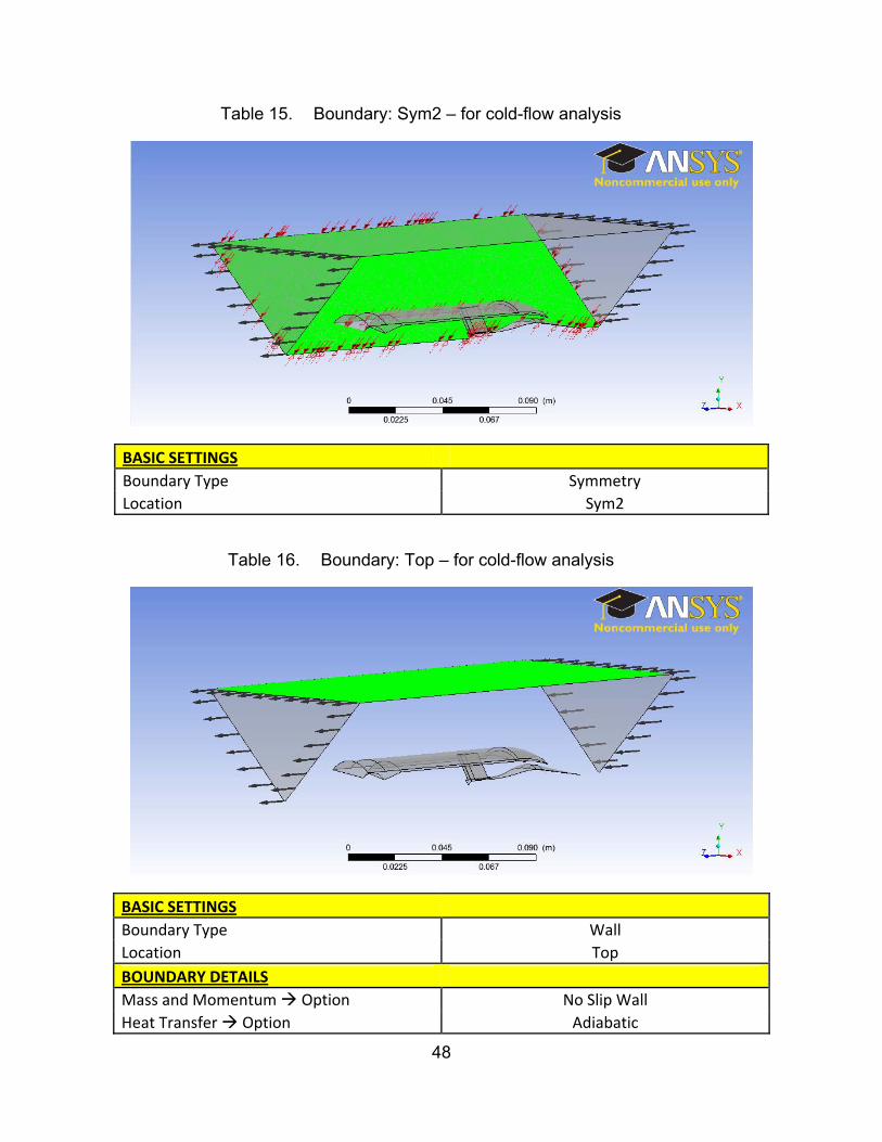
Table 15. Boundary: Sym2 – for cold-flow analysis

BASIC SETTINGS


Location Sym2

Table 16. Boundary: Top – for cold-flow analysis

BASIC SETTINGS

Boundary Type Wall

Location Top

BOUNDARY DETAILS

Mass and Momentum Option No Slip Wall

Heat Transfer Option Adiabatic

49

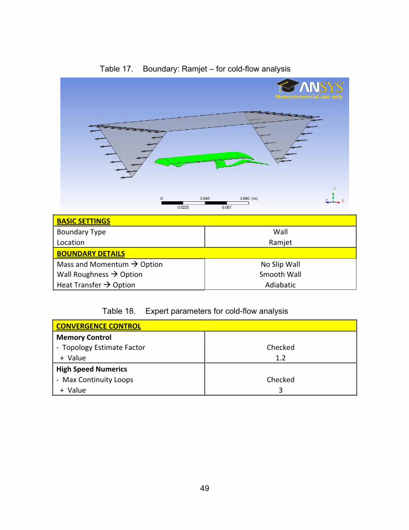
Table 17. Boundary: Ramjet – for cold-flow analysis

BASIC SETTINGS

Boundary Type Wall

Location Ramjet

BOUNDARY DETAILS

Mass and Momentum Option No Slip Wall Wall Roughness Option Smooth Wall


Table 18. Expert parameters for cold-flow analysis

CONVERGENCE CONTROL

Memory Control

‐ Topology Estimate Factor Checked

+ Value 1.2

High Speed Numerics

‐ Max Continuity Loops Checked

+ Value 3

50

Table 19. Solver control settings for cold-flow analysis

BASIC SETTINGS

Advection Scheme ‐‐> Option High Resolution

Turbulence Numerics ‐‐> Option High Resolution

Convergence Control

‐ Min. Iterations 1 ‐ Max. Iterations 1000 ‐ Fluid Timescale Control + Timescale Control Local Timescale Factor

+ Local Timescale Factor 3 Convergence Criteria

‐ Residual Type RMS

‐ Residual Target 1.00E‐06

ADVANCE OPTIONS

Compressibility Control Checked

‐ High Speed Numerics Checked

A3. OTHER NOTES

1. Time-stepping

As seen in the CFX-PRE setup section, a local timescale control with a factor of

3 was used to start the simulation. As the simulation stabilizes, the timescale control

was switched to automatic timescale control with a timescale factor of 1. Subsequently,

the timescale factor was also ramped progressively to a factor of 3 to reduce the time

taken for the results to converge. These changes in time scaling can be performed on

the fly with the “Edit Run in Progress” function in CFX-POST.

51

APPENDIX B – RESULTS FOR COLD-FLOW CFD ANALYSES

B1. MACH NUMBER PROFILE

Nozzle Throat Area Mach Number Profile Plot

Default Sizing

10% Reduction

20% Reduction

30% Reduction

40% Reduction

52

B2. PRESSURE PROFILE

Nozzle Throat Area Mach Number Profile Plot

Default Sizing

10% Reduction

20% Reduction

30% Reduction

40% Reduction

53

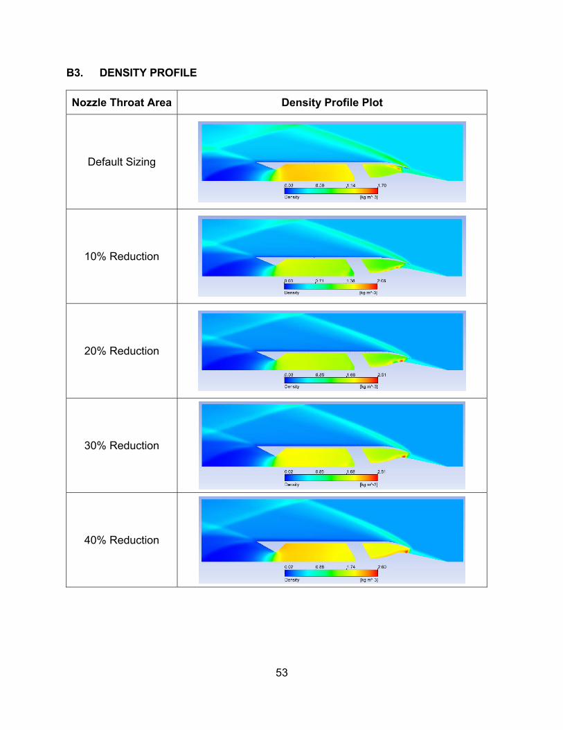
B3. DENSITY PROFILE

Nozzle Throat Area Density Profile Plot

Default Sizing

10% Reduction

20% Reduction

30% Reduction

40% Reduction

54

B4. STREAMLINE PLOT

Nozzle Throat Area

Streamline Plot

Default Sizing

10% Reduction

20% Reduction

30% Reduction

40% Reduction

55

B5. SHOCK INDICATOR PLOT

Nozzle Throat Area Shock Indicator Plot Remarks

Default Sizing Oblique shock

downstream the lip of the inlet cowl.

10% Reduction

Oblique shock downstream the lip of the

inlet cowl.

20% Reduction Oblique shock

downstream the lip of the inlet cowl.

30% Reduction

Shock on lip of inlet cowl. Flow downstream of shock is subsonic.

However, shock is not truly normal to flow.

40% Reduction

Normal shock formed upstream the lip of the

inlet cowl. Flow spillage. Sub-critical operation.

Legend:

56

B6. DRAG COEFFICIENT COMPUTATION

Drag induced on quarter - cut ramjet model = 6.70959 N

Total drag on full ramjet model (D) = 6.70959 × 4 = 26.838 N

0.03340Cross-section radius of ramjet = m

2

0.02Cross-section area of ramjet (A) = πR = π23340 -4 2= 8.762×10 m

2

Free stream velocity (V) = 661 m/s

3Free stream air density(ρ) = 0.377915 kg/m

DDrag coefficient = = 0.371

1 2ρV A2

57

APPENDIX C – DETAIL SETUP FOR CFD analysis on AIR INJECTION THROUGH THE TIP PORTS

C1. MESH SETUP

Table 20. Details of mesh setup for CFD analysis on air injection through tip ports

Defaults



Relevance 50

Sizing

Use Advance Size Function On: Proximity and Curvature Relevance Centre Fine Initial Size Seed Active Assembly Smoothing High

Transition Slow Span Angle Centre Fine

‐ Curvature Normal Angle 18 deg





‐ Max Face Size 0.0005 m ‐ Max Size 0.0005 m

‐ Growth Rate 1.1

Inflation




Advance

Shape Checking CFD Element Midside Nodes Dropped Extra Retries for Assembly Yes


58

Table 21. Details of mesh inflation settings for CFD analysis on air injection through tip ports

Scope


Geometry 1 body

Definition

Suppressed No Boundary Scoping Method Named Selections Boundary Ramjet Inflation Option Total Thickness ‐ Number of Layers 20 ‐ Growth Rate 1.05 ‐ Maximum Thickness 1e‐4m


Table 22. Details of face sizing settings for CFD analysis on air injection through tip ports

Scope

Scoping Method Named Selection

Named Selection Port

Definition

Suppressed No Type Element Size ‐ Element Size 0.000001 Behavior Soft

‐ Curvature Normal Angle Default ‐ Growth Rate Default

59

C2. CFX-PRE SETUP PARAMETERS

1. Domain: Default domain

BASIC SETTINGS

Location and Type






Domain Models



FLUID MODELS


Turbulence





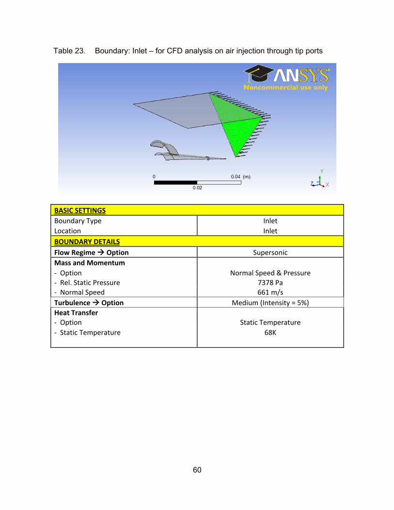
60

Table 23. Boundary: Inlet – for CFD analysis on air injection through tip ports

BASIC SETTINGS

Boundary Type Inlet

Location Inlet

BOUNDARY DETAILS


Mass and Momentum





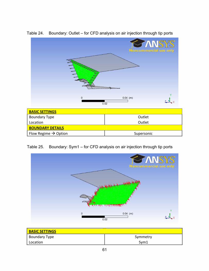
61

Table 24. Boundary: Outlet – for CFD analysis on air injection through tip ports

BASIC SETTINGS


Location Outlet

BOUNDARY DETAILS


Table 25. Boundary: Sym1 – for CFD analysis on air injection through tip ports

BASIC SETTINGS


Location Sym1

62

Table 26. Boundary: Sym2 – for CFD analysis on air injection through tip ports

BASIC SETTINGS


Location Sym2

Table 27. Boundary: Top – for CFD analysis on air injection through tip ports

BASIC SETTINGS

Boundary Type Wall

Location Top

BOUNDARY DETAILS



63

Table 28. Boundary: Ramjet – for CFD analysis on air injection through tip ports

BASIC SETTINGS

Boundary Type Wall

Location Ramjet

BOUNDARY DETAILS



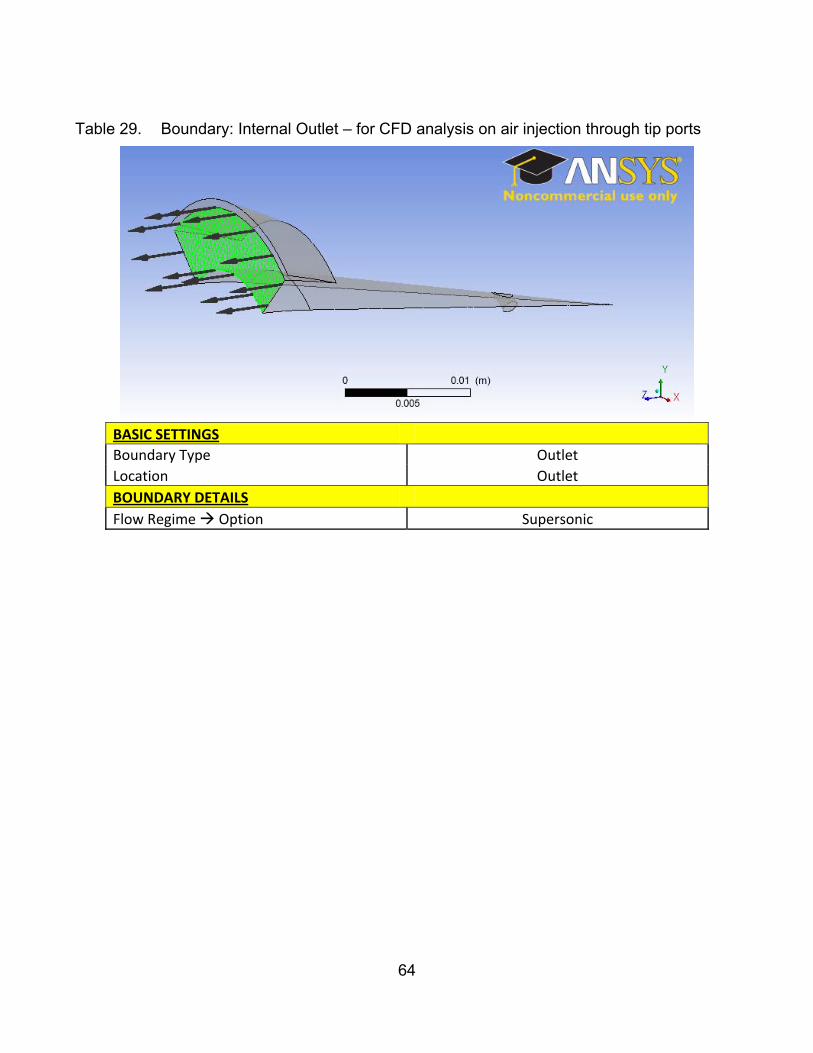
64

Table 29. Boundary: Internal Outlet – for CFD analysis on air injection through tip ports

BASIC SETTINGS


Location Outlet

BOUNDARY DETAILS


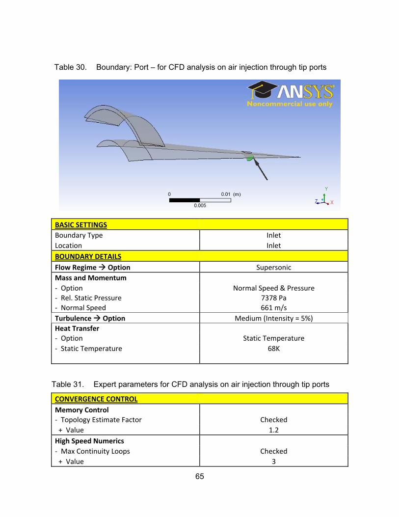
65

Table 30. Boundary: Port – for CFD analysis on air injection through tip ports

BASIC SETTINGS

Boundary Type Inlet

Location Inlet

BOUNDARY DETAILS


Mass and Momentum



Heat Transfer

‐ Option Static Temperature


Table 31. Expert parameters for CFD analysis on air injection through tip ports

CONVERGENCE CONTROL

Memory Control ‐ Topology Estimate Factor Checked

+ Value 1.2

High Speed Numerics


+ Value 3

66

Table 32. Solver control settings for CFD analysis on air injection through tip ports

BASIC SETTINGS

Advection Scheme ‐‐> Option High Resolution

Turbulence Numerics ‐‐> Option High Resolution

Convergence Control

‐ Min. Iterations 1 ‐ Max. Iterations 1000 ‐ Fluid Timescale Control + Timescale Control Local Timescale Factor




ADVANCE OPTIONS



C3. OTHER NOTES

1. Time-stepping



was switched to automatic timescale control with a timescale factor of 1. This change in

time scaling can be performed on the fly with the “Edit run in progress” function in CFX-

POST.

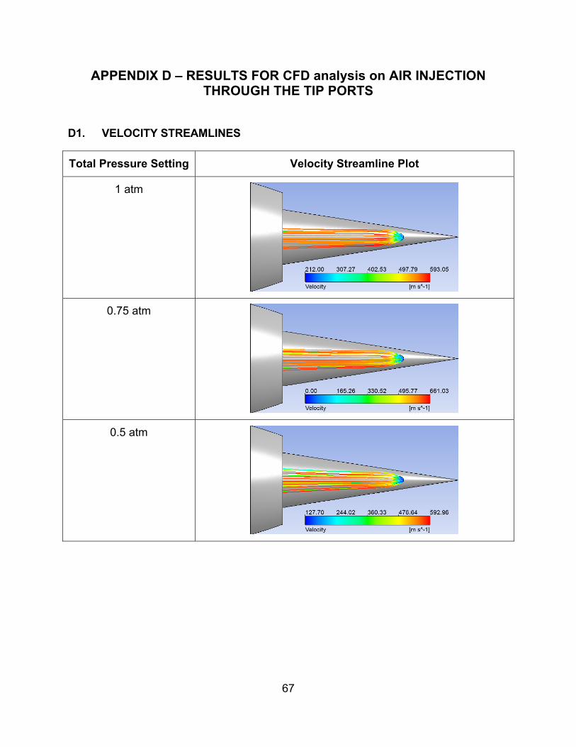
67

APPENDIX D – RESULTS FOR CFD analysis on AIR INJECTION THROUGH THE TIP PORTS

D1. VELOCITY STREAMLINES

Total Pressure Setting Velocity Streamline Plot

1 atm

0.75 atm

0.5 atm

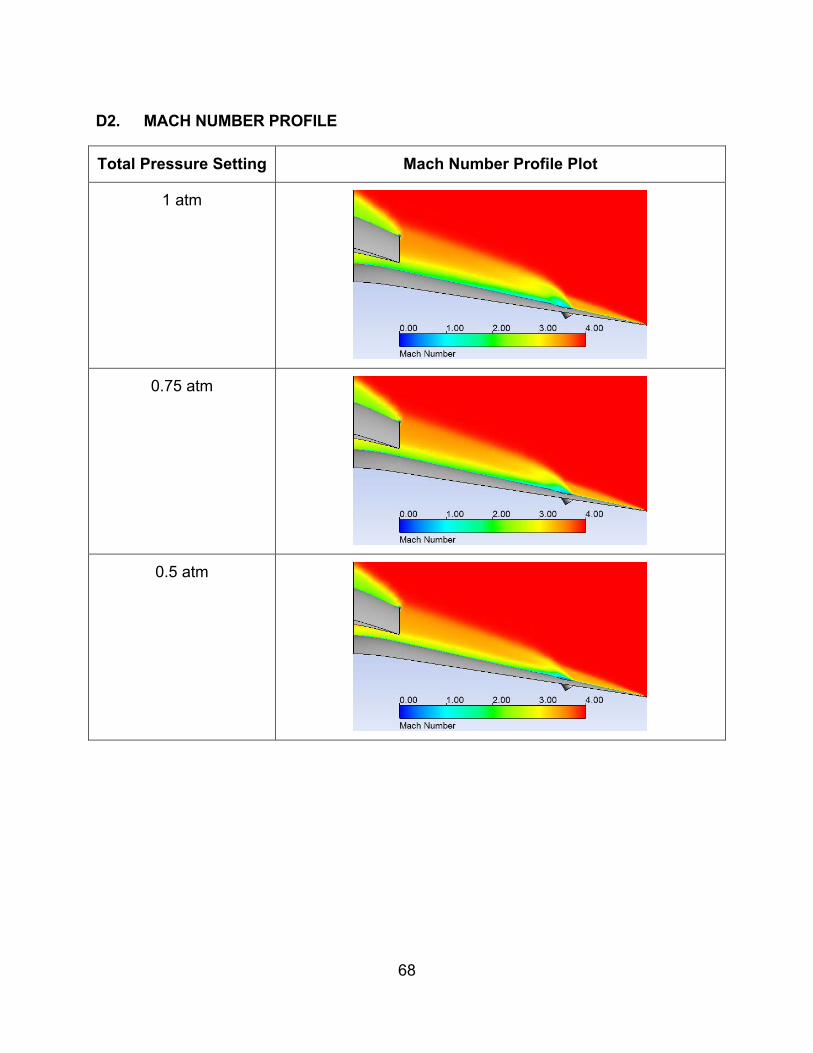
68

D2. MACH NUMBER PROFILE

Total Pressure Setting Mach Number Profile Plot

1 atm

0.75 atm

0.5 atm

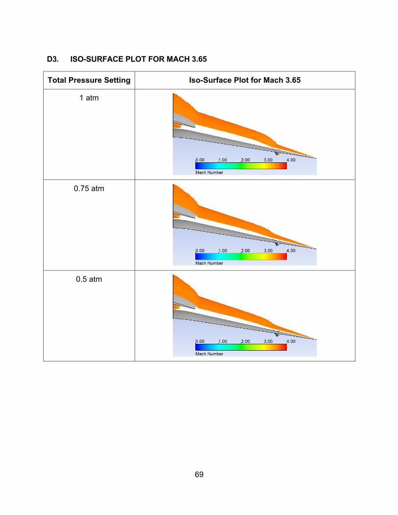
69

D3. ISO-SURFACE PLOT FOR MACH 3.65

Total Pressure Setting Iso-Surface Plot for Mach 3.65

1 atm

0.75 atm

0.5 atm

70


71

APPENDIX E – STOICHIOMETRIC CALCULATION

E1. STOICHIOMETRIC FUEL-AIR RATIO

Assumed Composition of Air:

23.2% Oxygen, 76.8% Nitrogen

1 Mole of Oxygen, 3.31 Mole of Nitrogen

Basic Equation for Stoichiometric Hydrogen – Air Combustion:

H2 + (3.31 N2 + O2) 2 H2O + 3.31 N2

Molar Mass of H2 = 2.016 x 2 = 4.032

Molar Mass of O2 = 31.99 x 1 = 31.99

Molar Mass of N2 = 28.01 x 3.31 = 92.7131

Stoichiometric Fuel-Air Ratio

4.032 : (92.7131+31.99)

4.031 : 124.7031

1: 30.94

72

E2. REQUIRED MASS FLOW FOR HYDROGEN

Based on International Standard Atmosphere conditions at altitude of 18000m:

Temperature = T∞ = 216.65 K

Pressure = P∞ = 7504.8 Pa

Velocity at Mach 4 = 4× γRT = 4× 1.4×287×216.65 =1180.17m / s

air air captured air

air -4

air air

-4

m =ρ A V

P= 1180.173.536×10R T

7504.8= 1180.173.536×10

287×216.65= 0.05037 kg / s

fuel fuel

air

-3fuel

m m1 1= =

m 30.94 0.05037 30.94

m =1.628×10 kg / s

73

APPENDIX F – DETAIL SETUP FOR COMBUSTION CFD ANALYSIS

F1. MESH SETUP

Table 33. Details of mesh setup for combustion analysis

Defaults



Relevance 50

Sizing

Use Advance Size Function On: Proximity and Curvature

Relevance Center Fine

Initial Size Seed Active Assembly

Smoothing High

Transition Slow

Span Angle Center Fine

‐ Curvature Normal Angle Default





‐ Max Face Size 0.0004 m

‐ Max Size 0.0004 m

‐ Growth Rate 1.1

Inflation




Advance

Shape Checking CFD

Element Midside Nodes Dropped

Extra Retries for Assembly Yes


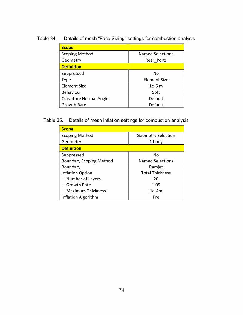
74

Table 34. Details of mesh “Face Sizing” settings for combustion analysis

Scope

Scoping Method Named Selections

Geometry Rear_Ports

Definition

Suppressed No

Type Element Size

Element Size 1e‐5 m

Behaviour Soft

Curvature Normal Angle Default

Growth Rate Default

Table 35. Details of mesh inflation settings for combustion analysis

Scope


Geometry 1 body

Definition

Suppressed No Boundary Scoping Method Named Selections Boundary Ramjet Inflation Option Total Thickness ‐ Number of Layers 20 ‐ Growth Rate 1.05 ‐ Maximum Thickness 1e‐4m


75

F2. CFX-PRE SETUP PARAMETERS

Table 36. Default domain for combustion analysis

BASIC SETTINGS

Location and Type



Fluid and Particles Definition for Fluid 1 ‐ Option: Material Library ‐ Material Hydrogen Air Mixture ‐ Morphology Continuous Fluid

Domain Models

‐ Pressure Reference Pressure 0 Pa

‐ Buoyancy Model Option Non‐Buoyant

‐ Domain Motion Option Stationary

FLUID MODELS


Turbulence





Components Model Component

‐ H2 Option Transport Equation

‐ H2O Option Transport Equation ‐ N2 Option Constraint

‐ O2 Option Transport Equation

76

Table 37. Boundary: Inlet – for combustion analysis

BASIC SETTINGS

Boundary Type Inlet Location Inlet

BOUNDARY DETAILS


Mass and Momentum ‐ Option Normal Speed & Pressure ‐ Rel. Static Pressure 7504.8 Pa ‐ Normal Speed 1180.17 m/s


Heat Transfer ‐ Option Static Temperature ‐ Static Temperature 216.65K

Components Model Component

‐ H2 Option Mass Fraction + Mass Fraction 0 ‐ H2O Option Mass Fraction + Mass Fraction 0 ‐ O2 Option Mass Fraction

+ Mass Fraction 0.232

77

Table 38. Boundary: Outlet – for combustion analysis

BASIC SETTINGS


Location Outlet

BOUNDARY DETAILS


Table 39. Boundary: Sym1 – for combustion analysis

BASIC SETTINGS


Location Sym1

78

Table 40. Boundary: Sym2 – for combustion analysis

BASIC SETTINGS


Location Sym2

Table 41. Boundary: Ramjet – for combustion analysis

BASIC SETTINGS

Boundary Type Wall

Location Ramjet

BOUNDARY DETAILS



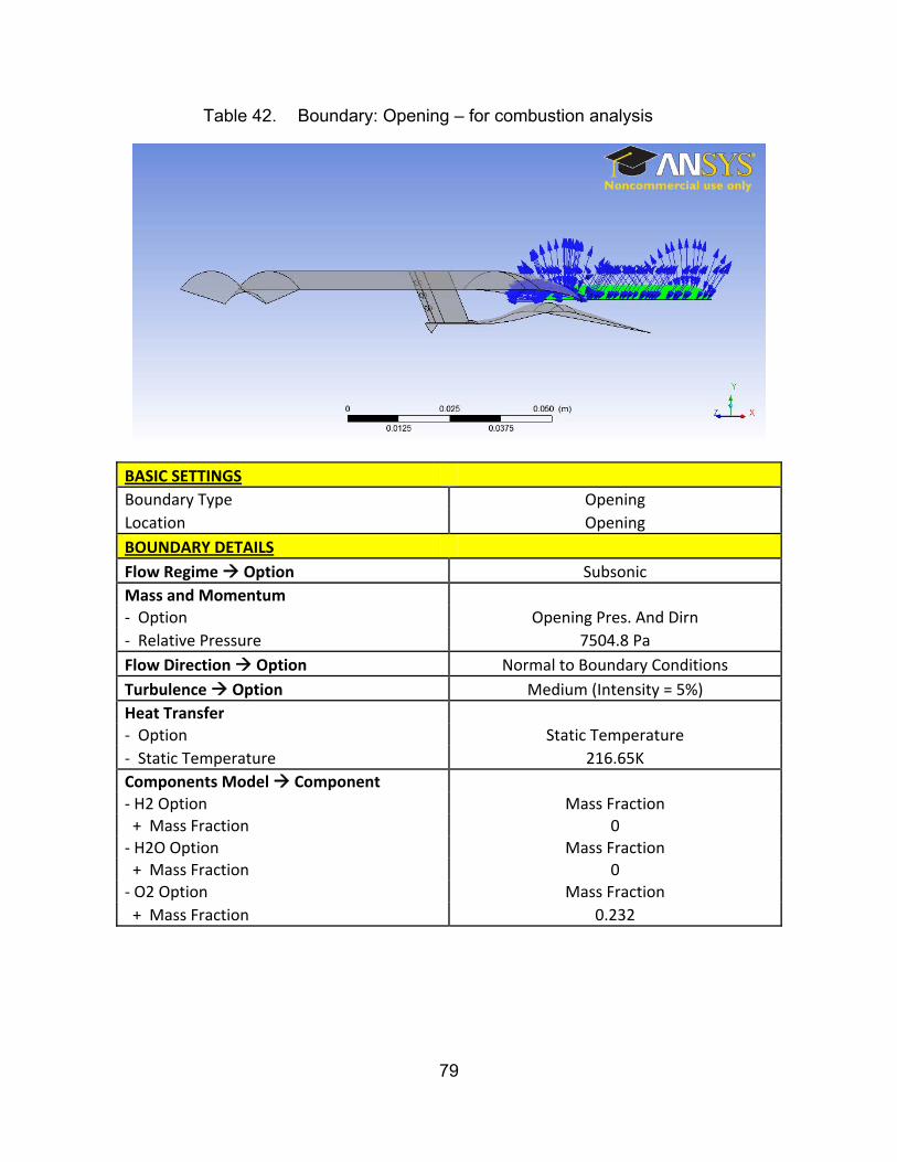
79

Table 42. Boundary: Opening – for combustion analysis

BASIC SETTINGS

Boundary Type Opening

Location Opening

BOUNDARY DETAILS

Flow Regime Option Subsonic

Mass and Momentum ‐ Option Opening Pres. And Dirn

‐ Relative Pressure 7504.8 Pa

Flow Direction Option Normal to Boundary Conditions



‐ Static Temperature 216.65K

Components Model Component ‐ H2 Option Mass Fraction + Mass Fraction 0

‐ H2O Option Mass Fraction + Mass Fraction 0 ‐ O2 Option Mass Fraction


80

Table 43. Boundary: Rear_Ports – for combustion analysis

BASIC SETTINGS

Boundary Type Inlet

Location Rear_Ports

BOUNDARY DETAILS

Flow Regime Option Subsonic

Mass and Momentum ‐ Option Normal Speed

‐ Normal Speed 50 m/s



‐ Total Temperature 300K

Components Model Component ‐ H2 Option Mass Fraction + Mass Fraction 1 ‐ H2O Option Mass Fraction + Mass Fraction 0 ‐ O2 Option Mass Fraction

+ Mass Fraction 0

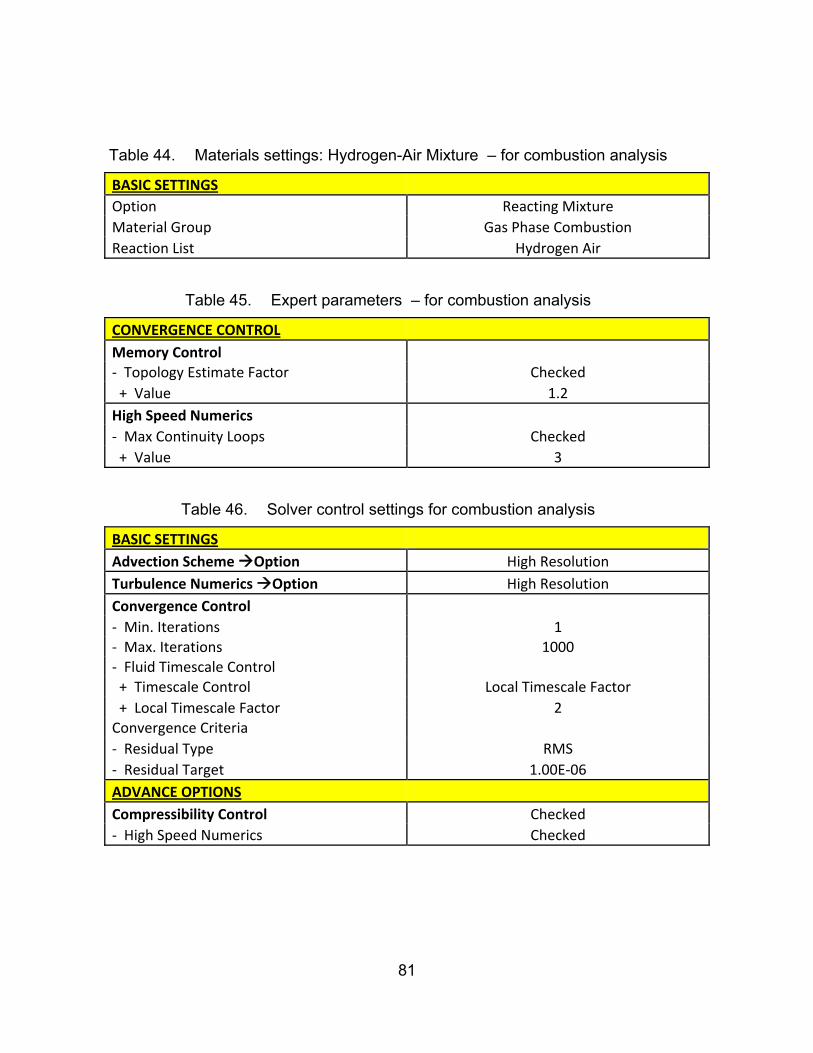
81

Table 44. Materials settings: Hydrogen-Air Mixture – for combustion analysis

BASIC SETTINGS

Option Reacting Mixture

Material Group Gas Phase Combustion

Reaction List Hydrogen Air

Table 45. Expert parameters – for combustion analysis

CONVERGENCE CONTROL

Memory Control

‐ Topology Estimate Factor Checked

+ Value 1.2

High Speed Numerics


+ Value 3

Table 46. Solver control settings for combustion analysis

BASIC SETTINGS

Advection Scheme Option High Resolution

Turbulence Numerics Option High Resolution

Convergence Control

‐ Min. Iterations 1 ‐ Max. Iterations 1000 ‐ Fluid Timescale Control

+ Timescale Control Local Timescale Factor




ADVANCE OPTIONS



82

Table 47. Global initialization for combustion analysis

GLOBAL SETTINGS

Initial Conditions

Velocity Type Cartesian

Cartesian Velocity Components Option Automatic

Static Pressure Option Automatic

Temperature Option Automatic

Turbulence Option Medium (Intensity =5%)

Component Details ‐ H2 Option Automatic ‐ H2O Option Automatic with Value


‐ O2 Option Automatic with Value + Mass Fraction 0.232

Table 48. Activating combustion in domain for combustion analysis

FLUID MODELS

Combustion

‐ Option Eddy Dissipation

‐ Eddy Dissipation Model Coefficient B 0.5


F3. OTHER NOTES

1. Mass-flow injection of Hydrogen fuel

A low hydrogen injection velocity of 50 m/s was used to start the simulation. This

velocity was ramped up incrementally to 400 m/s. After the computation stabilized at

400 m/s, the combustion settings in the domain setup was activated.

2. Time-stepping



was switched to automatic timescale control with a timescale factor of 1. Subsequently,

the timescale factor was ramped progressively to a factor of 3 to reduce the time taken

for the results to converge. These changes in time scaling can be performed on the fly

with the “Edit run in progress” function in CFX-POST.

83

APPENDIX G – ENGINEERING DRAWINGS FOR RAMJET MODEL

Figure 38. Part drawing: Ramjet inlet nose cone (RJ – 1)

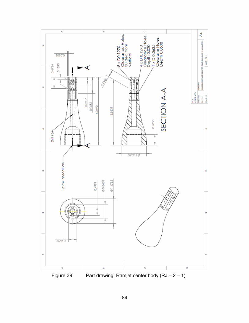
84

Figure 39. Part drawing: Ramjet center body (RJ – 2 – 1)

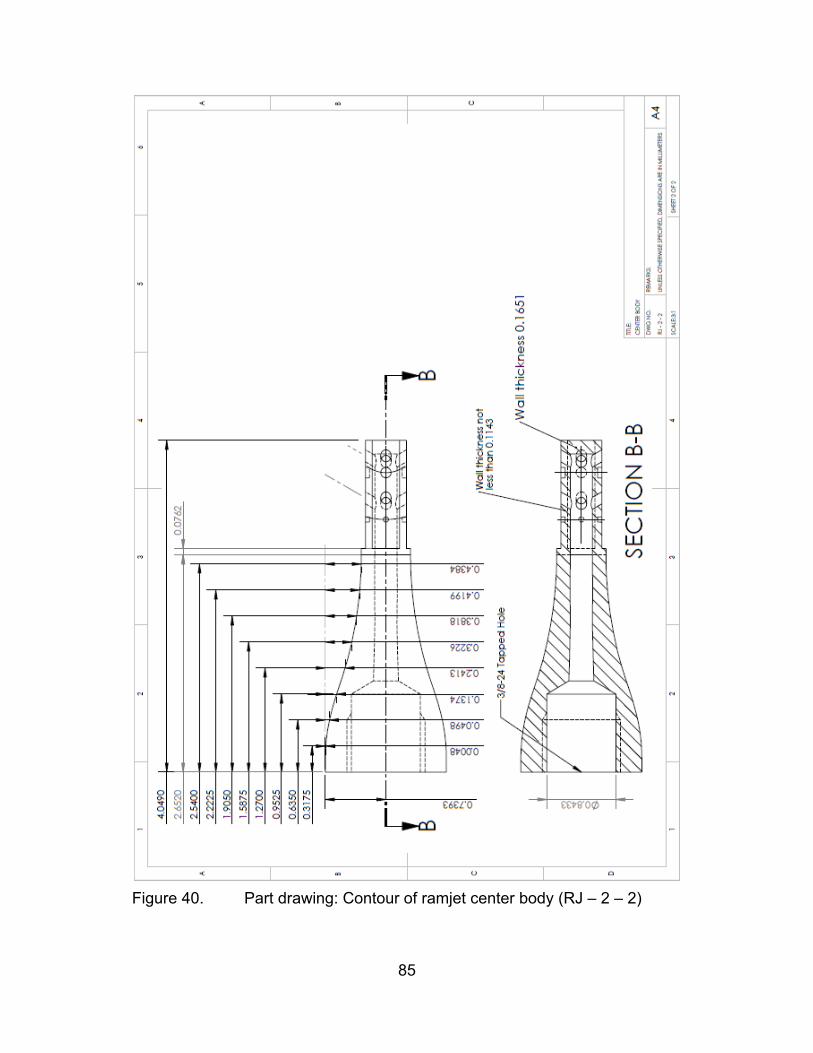
85

Figure 40. Part drawing: Contour of ramjet center body (RJ – 2 – 2)

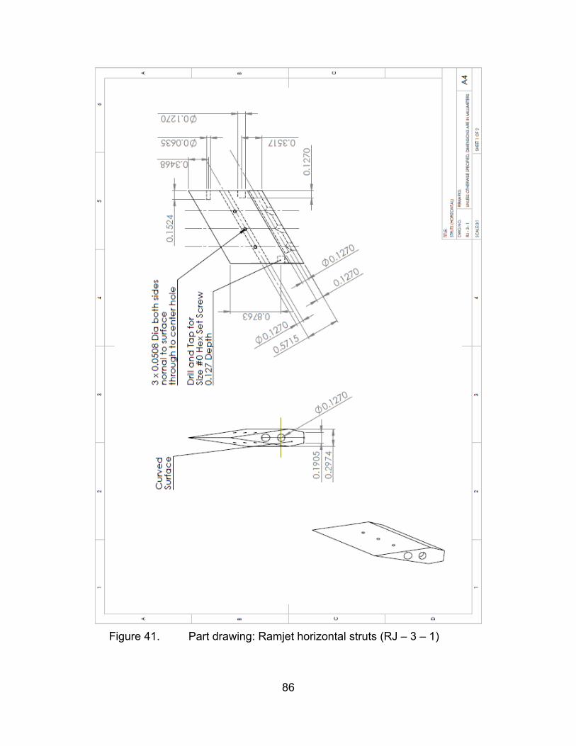
86

Figure 41. Part drawing: Ramjet horizontal struts (RJ – 3 – 1)

87

Figure 42. Part drawing: Ramjet horizontal struts (RJ – 3 – 2)

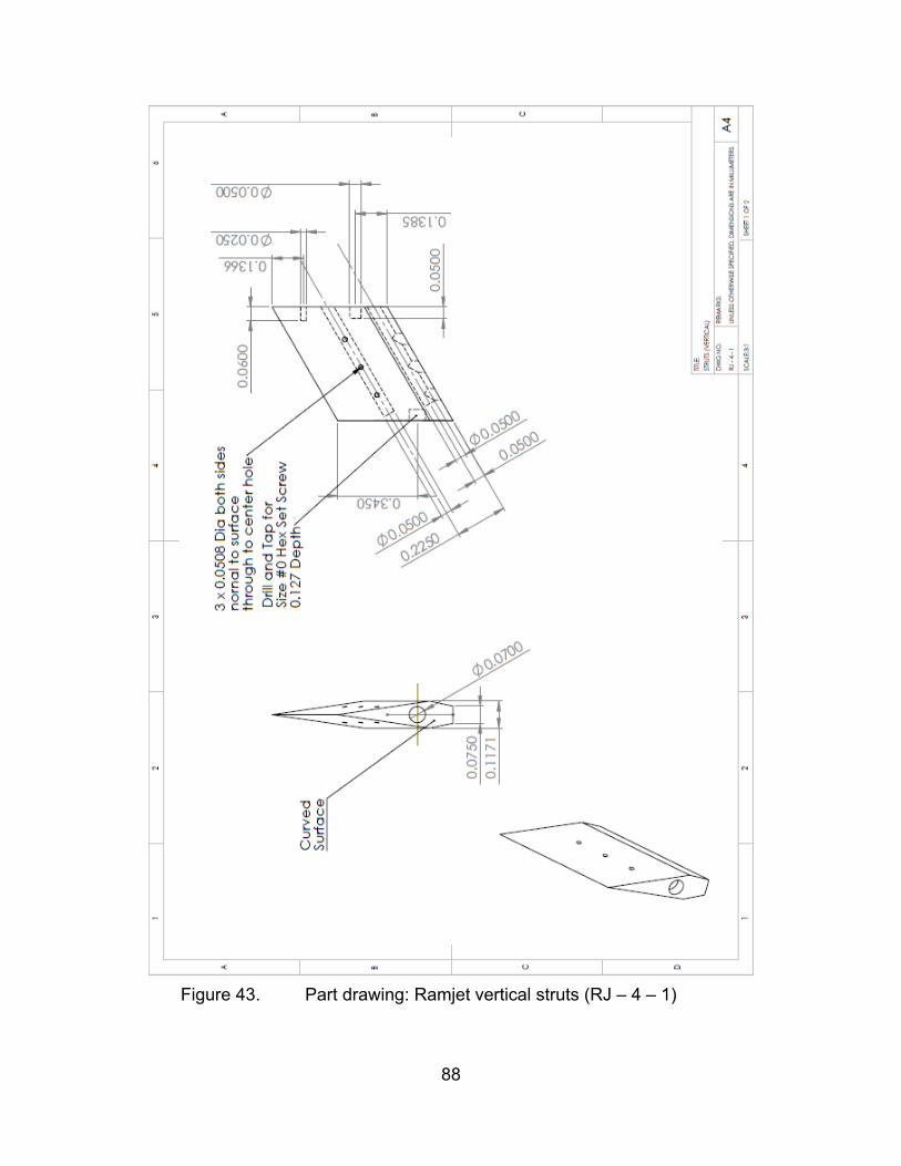
88

Figure 43. Part drawing: Ramjet vertical struts (RJ – 4 – 1)

89

Figure 44. Part drawing: Ramjet vertical struts (RJ – 4 – 2)

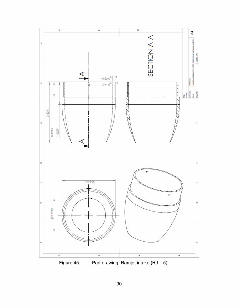
90

Figure 45. Part drawing: Ramjet intake (RJ – 5)

91

Figure 46. Part drawing: Ramjet combustion chamber (RJ – 6)

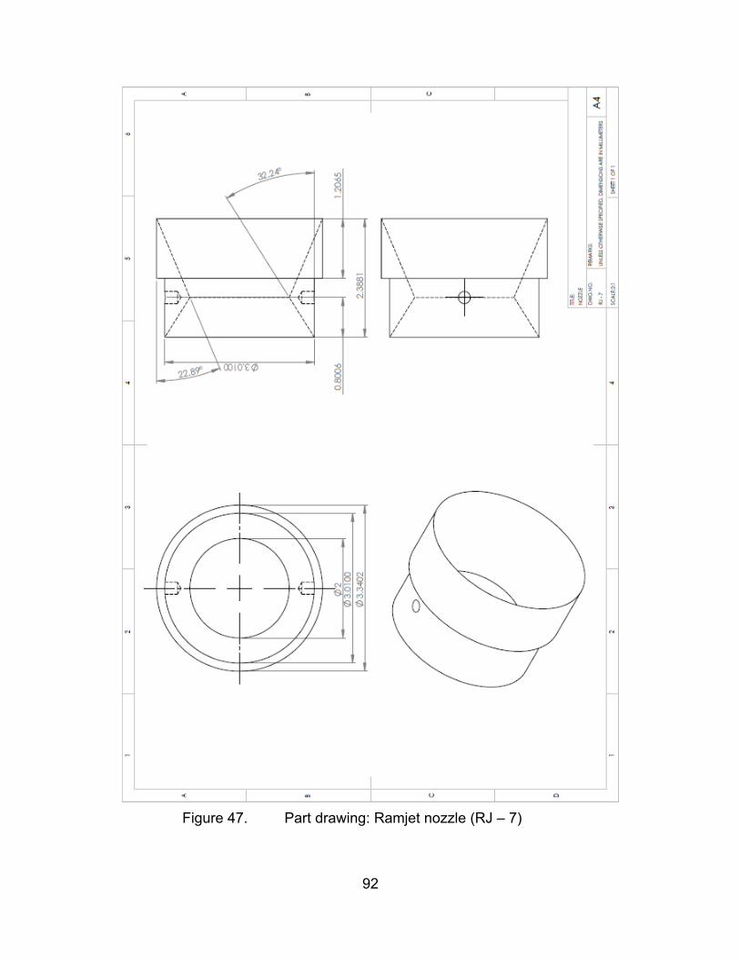
92

Figure 47. Part drawing: Ramjet nozzle (RJ – 7)

93

Figure 48. Part drawing: Flexure (RJ – 8 – 1)

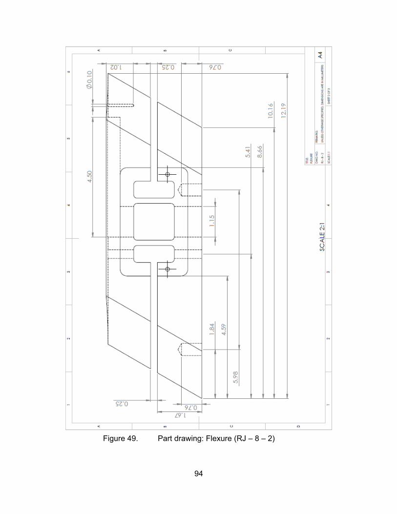
94


95


96


97

APPENDIX H – Details for Strain Gauges used

Manufacturer: Micro-Measurements (Vishay Precision Group) Model: WK – 13 – 062AP – 350 Description: Fully encapsulated Nickel-Chromium Alloy (K-Alloy) Operating Temperature Range: -269°C to 290°C (Normal) -269°C to 400°C (Normal)

Resistance: Fatigue Strain: Gauge Length: Overall Length: Grid Width: Overall Width: Matrix Length: Matrix Width:

350 Ω 2200µε 1.57 mm 2.90 mm 1.57 mm 1.57 mm 6.6 mm 4.1 mm

Details used here are extracted from the Manufacturer’s Data Sheet, available for download online at: http://www.vishaypg.com/docs/50003/precsg.pdf

98


99

APPENDIX I – DETAILED EXPERIMENT PROCEDURES FOR DRAG MEASUREMENT EXPERIMENT

I1. CALIBRATION OF SIGNALS CONDITIONING SYSTEM

Note: Unless otherwise stated, all PIN references refers to the PIN on the CALEX

8610 Backplane.

1. Set up the signals conditioning system.

a. On the CALEX 163MK Bridgesensor.

i. Set dip switch 1 to OFF.

ii. Set dip switch 2 and 3 to ON, 4 and 5 to OFF.

b. On the CALEX 8610 backplane, set dip switch 6 to ON and 7 to

OFF.

c. Connect the 110V A.C. power input to L1, L2 and G.

d. Set the input offset to 0V.

i. Short PIN 2 (Sense+) and PIN 3 (Bridge+).

ii. Short PIN 11(Common) and PIN and PIN 12 (Sense-).

iii. Turn on the power supply.

iv. Monitor the voltage drop across PIN 3 and 10 and tune RP2

on the Bridgesensor until the required excitation voltage to 4V DC is obtained.

v. Turn off the power supply.

2. Set the input offset of the amplifier to 0V.

a. Connect PIN 13 (In-) and PIN 14 (In+) to PIN 10 (Common).

b. Turn on the power supply.

c. Monitor the voltage of PIN 16 (Amplifier Output).

d. On the Bridgesensor, tune RP3 (Input offset trim port) to get a 0V.

e. Turn off the power supply.

100

f. The input offset is now 0V.

3. Set the gain of the amplifier to 100.

a. Disconnect PIN 14 (In+) from PIN 10 (Common).

b. Feed 1mV into PIN 14 (In+).

c. Turn on the power supply.

d. Monitor the voltage drop across PIN 16 (amplifier output) and PIN

10.

e. Tune RP5 (coarse gain adjustment) and RP4 (fine gain adjustment)

on the Bridgesensor until the voltage drop across PIN 16 and PIN 10 is 0.1V.

f. Turn off the power supply.

g. The gain of the amplifier is now set to 100.

I2. LOAD CELL CALIBRATION

1. Set up the load cell as shown in Figure 51.

Figure 51. Wiring diagram for load cell calibration

2. Apply a 1kg mass to the load cell and note the voltage response on the

voltmeter.

3. Repeat step 2 for 2kg - 5kg mass.

I3. STRAIN GAUGE CALIBRATION

1. Balancing the Wheatstone bridge.

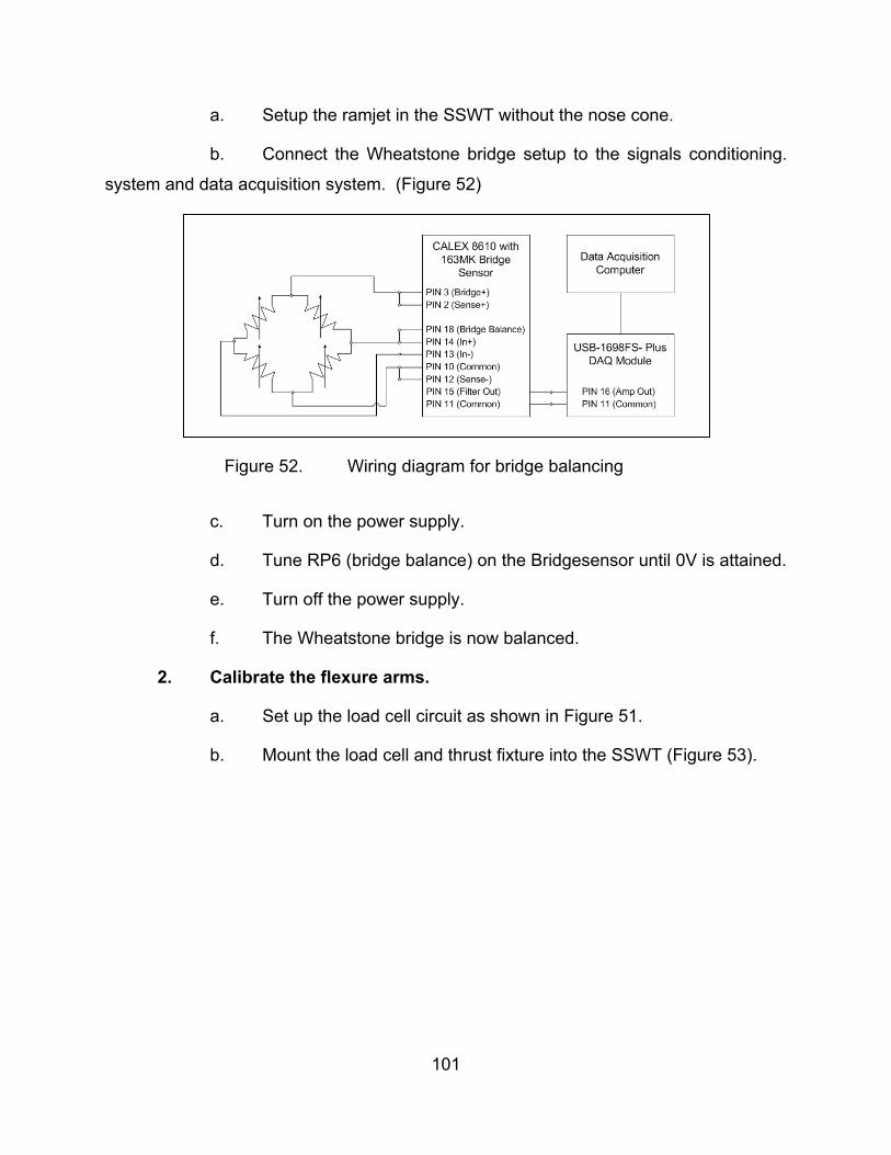
101

a. Setup the ramjet in the SSWT without the nose cone.

b. Connect the Wheatstone bridge setup to the signals conditioning.

system and data acquisition system. (Figure 52)

Figure 52. Wiring diagram for bridge balancing


d. Tune RP6 (bridge balance) on the Bridgesensor until 0V is attained.

e. Turn off the power supply.

f. The Wheatstone bridge is now balanced.

2. Calibrate the flexure arms.

a. Set up the load cell circuit as shown in Figure 51.

b. Mount the load cell and thrust fixture into the SSWT (Figure 53).

102

Figure 53. Load cell and thrust fixture mounted in SSWT with ramjet model


d. Turn the jackscrew until the equivalence of a 1kg mass force is

observed on the voltmeter.

e Monitor the voltage drop across PIN 15 (Filter out) and PIN 10

(Common).

d. Repeat 2d and 2e with the equivalence of a 2kg, 3kg, 4kg and 5kg

mass force.

e. Determine the force and voltage drop relationship for the strain

gauges.

I4. DRAG MEASUREMENT

1. Drag measurement.

a. Setup the ramjet in the SSWT.

Mounted Ramjet Thrust Fixture Load Cell

Wooden Reaction Block with Jackscrew

103

b. Connect the Wheatstone bridge setup to the signals conditioning

system and data acquisition system (Figure 52).

c. Start the SSWT to Mach 4.

d. Log the voltage drop measurements with the TracerDAQ software.

2. Base on the mass-voltage drop relationship obtained in C2, determine the

drag force induced on the ramjet and inner flexures.

104


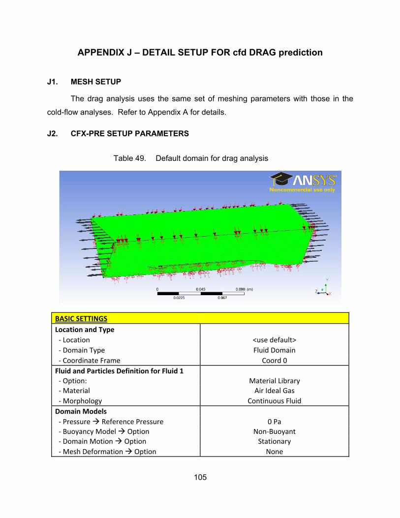
105

APPENDIX J – DETAIL SETUP FOR cfd DRAG prediction

J1. MESH SETUP

The drag analysis uses the same set of meshing parameters with those in the

cold-flow analyses. Refer to Appendix A for details.

J2. CFX-PRE SETUP PARAMETERS

Table 49. Default domain for drag analysis

BASIC SETTINGS

Location and Type






Domain Models



106

FLUID MODELS


Turbulence





Table 50. Boundary: Flexure – for drag analysis

BASIC SETTINGS

Boundary Type Wall

Location Top

BOUNDARY DETAILS



3. Other Setup Parameters

The other boundary conditions and setup parameters are the same as those

used in the cold-flow analyses. Refer to Appendix A for details.

107

J3. OTHER NOTES

1. Time-stepping

As seen in the CFX-PRE setup section, a local timescale control with a

factor of 3 was used to start the simulation. As the simulation stabilizes, the

timescale control was switched to automatic timescale control with a timescale

factor of 1. Subsequently, the timescale factor was ramped progressively to a

factor of 3 to reduce the time take for the results to converge. These changes in

time scaling can be performed on the fly with the “Edit run in progress” function in

CFX-POST.

108


109

LIST OF REFERENCES

[1] K. M. Ferguson, Design and cold flow evaluation of a miniature mach 4 ramjet, Monterey, CA, 2003.

[2] W. T. Khoo, Cold flow drag measrement and nmerical performance prediction of a miniature ramjet

at mach 4, Monterey, CA, 2003.

[3] "ANSYS CFX‐SOLVER theory guide," [Online]. Available:

https://www1.ansys.com/customer/content/documentation/140/cfx_thry.pdf. [Accessed 1 March

2012].

[4] J. E. Bardina, P. G. Huang and T. J. Coakley, Turbulence modeling validation, testing, and

development, 1997.

[5] F. R. Menter, "Two‐equation eddy‐viscosity turbulence models for engineering applications," AIAA

Journal, vol. 32, no. 8, pp. 1598‐1605, Aug. 1994.

110


111

INITIAL DISTRIBUTION LIST

1. Defense Technical Information Center Ft. Belvoir, Virginia 2. Dudley Knox Library Naval Postgraduate School Monterey, California 3. Hobson, Garth Department of Mechanical and Aerospace Engineering Naval Postgraduate School Monterey, California 4. Brophy, Christopher Department of Mechanical and Aerospace Engineering Naval Postgraduate School Monterey, California 5. COL Lim Soon Chia Defence Research and Technology Office Ministry of Defence Singapore 6. Yeo Tat Soon Temasek Defence Systems Institute National University of Singapore Singapore 7. Tan Lai Poh Temasek Defence Systems Institute National University of Singapore Singapore

Documents

Numerical Performance Prediction of a Miniature at Mach 4