Numerical Prediction of 8 May 2003 Oklahoma City Tornadic Supercell and Embedded Tornado using ARPS with the Assimilation of WSR-88D Radar

Data

Ming Xue1,2*, Ming Hu1,3, and Alexander D. Schenkman1

1Center for Analysis and Prediction of Storms and 2School of Meteorology

University of Oklahoma, Norman, OK 73072

3Cooperative Institute for Research Environmental Sciences University of Colorado at Boulder, Boulder, CO 80309

Submitted to Weather and Forecasting February 2013

Revised and Accepted August, 2013

*Corresponding Author Address:

Dr. Ming Xue, School of Meteorology, University of Oklahoma,

NWC Suite 2500 120 David Boren Blvd, Norman OK 73072

E-mail: mxue@ou.edu

ii

Abstract

The 8 May 2003 Oklahoma City tornadic supercell is predicted with the ARPS model using four nested grids with 9-km, 1-km, 100-m, and 50-m grid spacings. The Oklahoma City WSR-88D radar radial velocity and reflectivity data are assimilated through the ARPS 3DVAR and cloud analysis on the 1-km grid to generate an initial condition that includes a well-analyzed supercell and associated low-level mesocyclone. Additional 1-km experiments show that the use of radial velocity and the proper use of a divergence constraint in the 3DVAR play an important role in the establishment of the low-level mesocyclone during the assimilation and forecast. Assimilating reflectivity data alone failed to predict the mesocyclone intensification.

The 100-m grid starts from the interpolated 1-km control initial condition while the further nested 50-m grid starts from the 20 minute forecast on the 100-m grid. The forecasts on both grids cover the entire period of observed tornado outbreak, and successfully capture the development of tornadic vortices. A tornado on the 50-m grid reaches high-end F-3 intensity while the corresponding simulated tornado on the 100-m grid reaches F-2 intensity. The timing of tornadogenesis on both grids agrees with observations very well, although the predicted tornado was slightly weaker and somewhat shorter lived. The predicted tornado track parallels the observed damage track although is displaced northward by about 8 km. The predicted tornado vortices have realistic structures similar to those documented in previous theoretical, idealized modeling and some observational studies. The prediction of an observed tornado in a supercell with a similar degree of realism has not been achieved before.

1. Introduction

For the goal of increasing the lead time of warnings issued on severe weather hazards, and in particular on tornadoes, Stensrud et al. (2009; 2013) discuss the necessity of shifting from warn-on-detection to the warn-on-forecast paradigm where advanced warnings are issued based on high-resolution numerical prediction of severe convective storms and associated severe weather rather than relying on detections in current observations and extrapolation-based nowcasting. Although the average warning lead time for tornadoes has increased from 3 min in 1978 to 14 min in 2011 in the United States, this improvement has been mostly due to improved detection capability, especially from the deployment of the operational Doppler radar network. Despite the progresses, the average lead time for all tornadoes with positive warning lead time was stagnant at around 20 min during the period of 1986-2006 (Stensrud et al. 2013); suggesting the current approach based on the warn-on-detection paradigm has likely reached its limit in terms of improving tornado warning lead time. The time has come for shifting to the warn-on-forecast paradigm, whereby a much greater reliance will be placed on predictions by high-resolution convection-resolving numerical models that, by employing ensemble forecasting, can also provide probabilistic forecasting information (Stensrud et al. 2009; 2013).

The first step towards achieving the warn-on-forecast goals for tornadoes is to be able to accurately initialize and predict the parent thunderstorms that spawn tornadoes. This by itself remains a significant challenge (Sun et al. 2013; Stensrud et al. 2013). In recent years, a significant number of studies have been devoted to the initialization of tornadic supercell storms through advanced radar data assimilation and in some cases also examined the subsequent forecasts at 1 to 3 km grid spacing (e.g., Xue et al. 2003; Dowell et al. 2004; Hu et al. 2006a; Hu and Xue 2007; Jung et al. 2012; Dawson et al. 2012; Tanamachi et al. 2013). While a successful prediction of a tornadic supercell with strong mid and low-level rotations suggests high potential of tornado formation, it does not directly predict tornado formation itself. Studies (e.g., Trapp 1999; Markowski et al. 2011) have shown that there is not necessarily a strong correlation between tornado occurrence with the existence and strength of the mid- and low-level mesocyclone, suggesting that the low-level rotation in the model may not be a reliable indicator of tornado potential. As such, it may be necessary to explicitly forecast the tornado-scale circulations to have a higher degree of certainty about the tornado potential. Given the small size of tornadoes, it is clear that one to two orders of magnitude higher spatial resolution are needed to resolve the tornado and associated circulations than what is needed to resolve the parent storm (Xue et al. 2007).

Existing studies that attempt to predict real tornadoes or tornado-like vortices are very limited. Mashiko et al. (2009) and Schenkman et al. (2012) are two of such studies known to the authors. By using quadruply nested grids, with the highest-resolution grid having a grid spacing of 50 m, Mashiko et al. (2009) were able to simulate convective storms in the outermost rainband of a land-falling typhoon that exhibited the characteristics of a mini-supercell; one of the simulated storms spawned a tornado whose genesis processes were analyzed in detail in their study. While actual tornadoes were observed within the outer rainband of this typhoon in a similar region, no direct comparison of the simulated tornado was made with the actual tornadoes. In Schenkman et al. (2012), a mesoscale convective system (MCS) that was rather accurately initialized by assimilating radar and other high-resolution observations on a 400-m grid, as documented in Schenkman et al. (2011), was further nested down to a 100-m grid. A

2

tornado-like vortex that matched an observed tornado was accurately simulated and the tornadogenesis processes were analyzed in detail.

In this study, we examine the ability of a nonhydrostatic numerical weather prediction model in predicting an observed F4-intensity tornado that developed within a supercell storm typical of the Central and Southern Great Plains of the United States. The case chosen is the tornadic supercell that occurred on 8 May 2003 in central Oklahoma, near Oklahoma City, which will be referred to as the OKC storm. A reasonably successful attempt to analyze and predict this storm was made by Hu and Xue (2007, hereafter HX07) using a model grid with a 3-km grid spacing that was nested inside a 9-km spacing grid. The study focused on the impact of and the sensitivity to the data assimilation method and the configurations of the intermittent assimilation cycles employed. The 9-km grid assimilated conventional observations while the 3-km grid assimilated data from the operational OKC radar. For their 3-km grid, using the ARPS 3DVAR and cloud analysis procedure (Xue et al. 2003; Hu et al. 2006a; Hu et al. 2006b), it was found that a 1-h-long assimilation window covering the entire initial stage of the storm together with a 10-min spin-up period before storm initiation produced the best results. HX07 also found significant sensitivity to the assimilation frequency and in-cloud temperature adjustment scheme used in the cloud analysis procedure. Despite reasonable success with the prediction of the overall storm over a 2.5 h period, due to the relatively coarse resolution used, the analyzed and predicted supercell was rather smooth in structure with only a slight indication of hook-echo structure in the low-level predicted reflectivity fields (see Fig. 4 in HX07). The circulation associated with the mid-level mesocyclone was present in their prediction but its diameter was too large (see Fig. 5 in HX07). Given the coarse resolution, it was difficult to determine if a tornado would develop or not in the simulated storm.

In this study, we refine the study of HX07 by performing radar data assimilation on a grid with a 1-km instead of 3-km grid spacing. The 1-km grid spacing is expected to much better resolve the structure and circulations of the supercell storm. Sensitivity experiments were performed to determine the assimilation configurations that gave the best storm prediction, and the predictions were evaluated through direct comparisons of predicted radial velocity and reflectivity with radar observations in the radar observation space.

After obtaining a reasonably accurate model prediction on the 1-km grid, we set off to address whether the model has the ability to directly predict the embedded tornado, given high enough resolution. As such, down-scaled forecasts at 100-m and 50-m grid spacings are conducted, starting from the final 1-km analysis. These two grids are successively nested in one-way interactive mode, with high-frequency boundary condition updates from successively coarser grids. Forecasts on these grids capture well the intensification of low-level rotation, leading to realistic tornadic signatures that compare well with observations. The timing of development of the simulated tornado on both grids is very close to observations. On the 50-m grid, the simulated tornado reaches F3 intensity. The structures of the simulated tornado are also examined to see how they compare with established conceptual models. Given the much lower computational cost of 3DVAR compared to that of ensemble-based data assimilation methods, the reasonably accurate model prediction on the 1-km grid and successful capturing of tornadic features on the 50-m grid are particularly encouraging, especially from an operational perspective.

The rest of this paper is organized as follows: Section 2 briefly introduces the 8 May 2003 tornadic thunderstorm case. The data assimilation and forecast experiment design is described in Section 3. Section 4 presents the results of data assimilation and forecasts on the 1-

3

km grid and the verification of the forecasts against radar observations. Section 5 focuses on the 50-m forecast and evaluates the structure, evolution, and track of the model-predicted tornado. A summary and discussion are presented in section 6. Apart from the important goal of evaluating the ability of a modern non-hydrostatic atmospheric model initialized using high-frequency radar observations in predicting a real supercell storm and its embedded tornadoes, another important goal of this paper is to establish, when possible, the physical realism of the simulated tornadoes in the model so as to provide high-frequency, high-resolution, gridded data sets for performing detailed diagnostic analyses on the tornadogenesis processes involved. The results of the diagnostic study will be reported in a separate paper (Schenkman et al. 2013).

2. Overview of the 8 May 2003 Oklahoma tornadic thunderstorm and tornado outbreak The OKC tornadic thunderstorm has been introduced in HX07. As in HX07, the

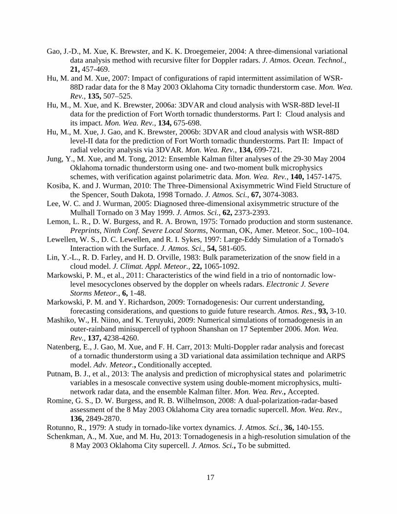
evolution of the OKC storm can be illustrated using a collage of low-level reflectivity whose values exceed 35 dBZ (Fig. 1). The storm was first observed as a weak echo by the operational Twin Lakes, Oklahoma City (KTLX) WSR-88D radar at 2040 UTC (hereafter, all times will be in UTC). It strengthened as it moved northeastward, taking on supercell characteristics. At around 2200, a pronounced hook appendage structure is found at the southwestern end of the storm, located northwest of Moore. The supercell storm propagated east-northeastward, and began to weaken after 2300, and dissipated by 0020 of 9 May. In addition to the main OKC storm, three smaller storms are seen in Fig. 1, labeled storms A, B, and C.

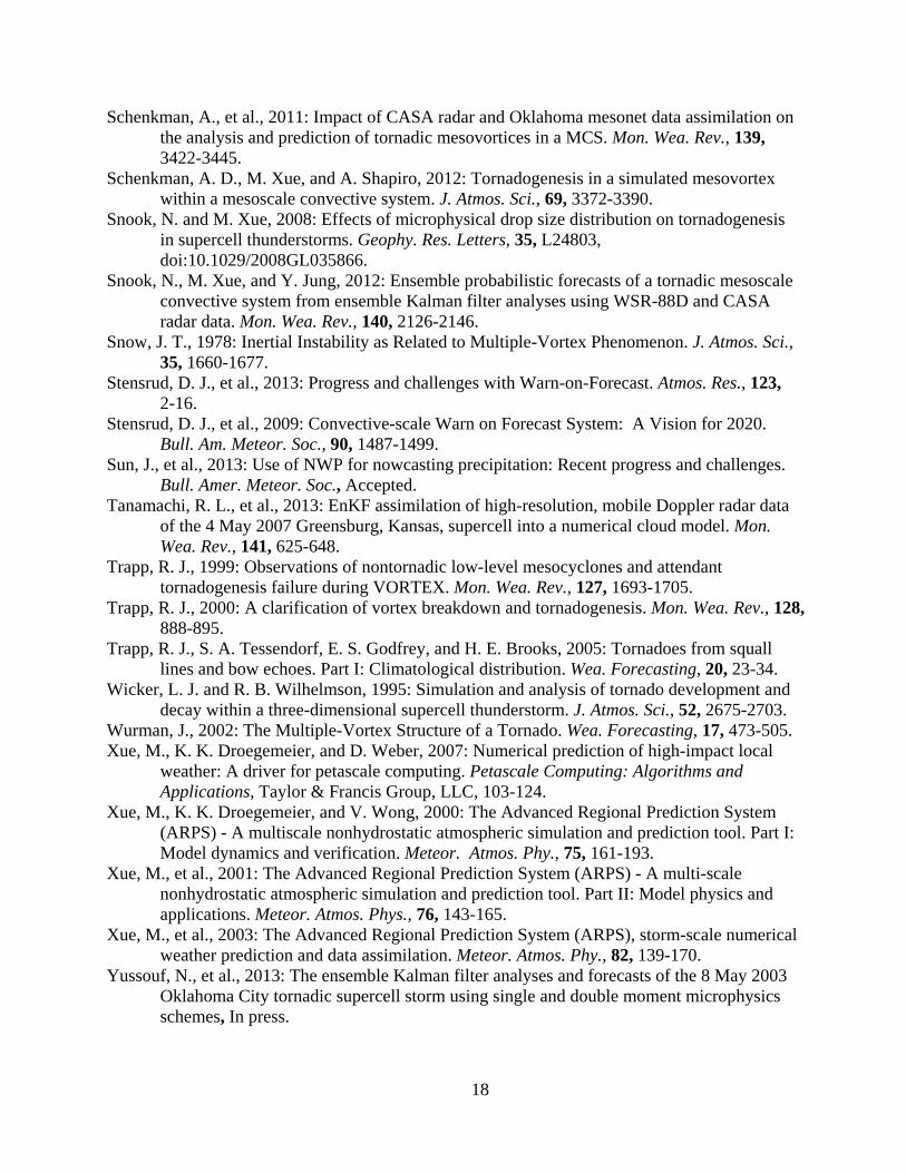
The tornado that struck the south side of Oklahoma City (hereafter, the OKC tornado) formed at 2210, tracked east-northeast on the ground for about 30 km, from Moore to Choctaw, Oklahoma, and dissipated at 2238 (Fig. 2). This tornado caused widespread F2-F4 damage. Prior to the genesis of the OKC tornado, two F0 tornadoes from the same storm were reported just southwest of Moore. Because these tornadoes were short-lived and weak, the focus of this study is on the long-track, high-impact OKC tornado. Additional discussion on this case can also be found in Romine et al. (2008).

3. Experiment setup

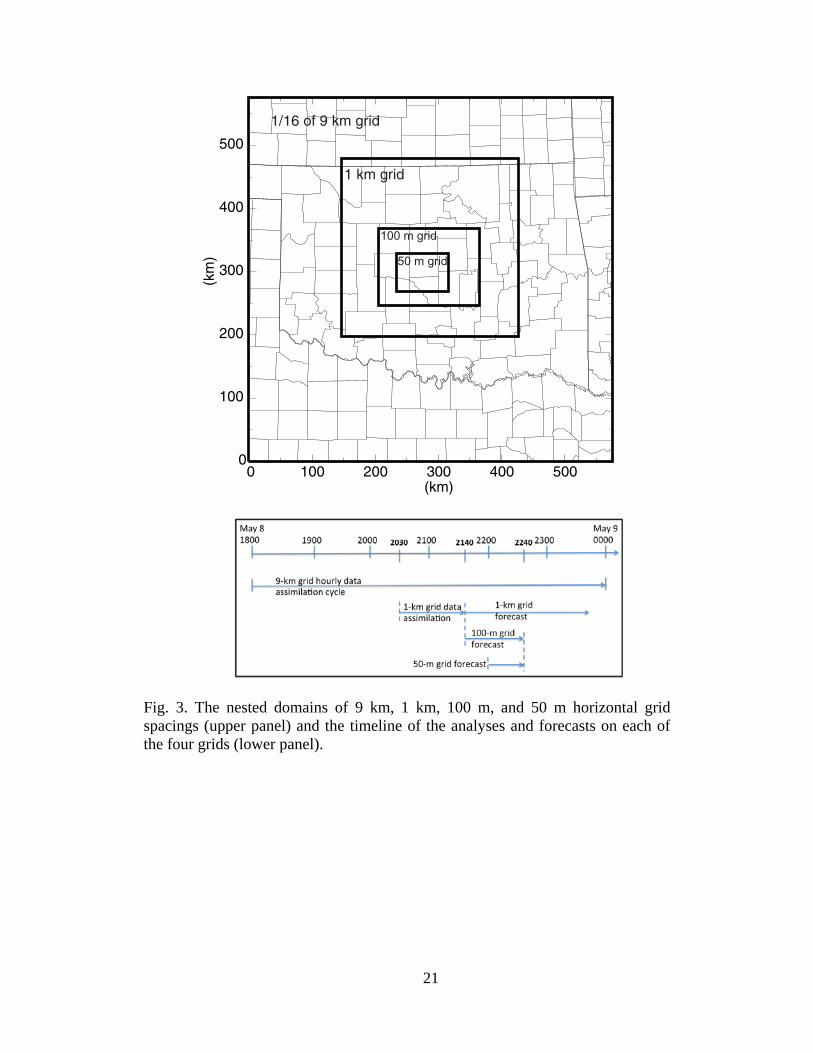
In this study, four one-way nested grids at horizontal grid spacings of 9 km, 1 km, 100 m and 50 m, respectively, are used (Fig. 3). All grids have 53 vertical levels with spacing that stretches from about 20 m near the surface to 770 m at the model top located at 21.1 km height.

The 9-km grid provides the initial analysis background and boundary conditions for the 1-km experiments. The 9-km grid covers an area of 2300 km × 2300 km and is identical to that described in HX07. The 9-km experiment includes 1-h assimilation cycles over a 6-h period from 1800, 8 May to 0000, 9 May, using the Advanced Regional Prediction System (ARPS, Xue et al. 2000; Xue et al. 2001) as the prediction model and its 3DVAR system (Xue et al. 2003; Gao et al. 2004) for data assimilation. The 1800 analysis of the NCEP Eta Model was used as the initial background and conventional observations including rawinsonde, wind profiler, surface weather station and Oklahoma Mesonet data were assimilated. A special Norman, Oklahoma sounding at 1800 was also included. The lateral boundaries were forced by the Eta 1800 forecasts at 3-h intervals.

The 1-km grid is 280 km × 280 km in size and covers central and northern Oklahoma (Fig. 3). Analogous to the 3-km experiments in HX07, radar data assimilation is performed on the 1-km grid. The 1-km control experiment, CNTL1km (Table 1), assimilates both radial

4

velocity (Vr ) and reflectivity (Z) data using the ARPS 3DVAR and cloud analysis scheme (Hu et al. 2006a; 2006b) through intermittent assimilation cycles. The assimilation window starts at 2030 and ends at 2140, covering the development stage of the OKC thunderstorm. Only data from a single operational WSR-88D radar at the Oklahoma City (KTLX) were assimilated in HX07 and in this study, which represents a more realistic operational setting even though data from an experimental WSR-88D radar in Norman Oklahoma and from a nearby Terminal Doppler Weather Radar (TDWR) were also available for this case. The use of single Doppler radar data also poses a more challenging data assimilation problem, for which assimilation cycling becomes more important (HX07, Natenberg et al. 2013). In this study, data from KTLX are assimilated every 5 minutes.

The KTLX data were first quality controlled and remapped from radar coordinates to the 1-km model grid. Time interpolation was performed on the data from individual scan elevations of successive scan volumes to obtain remapped data at 5 min intervals. Additional details on the procedures are described in HX07.

The temperature adjustment scheme used in the cloud analysis is the moist adiabat method (the MA scheme as designated in Hu et al. 2006a). Our control experiment CNTL1km is most similar to experiment 5B30E30MA of HX07 (see their Table 1), except for the increased resolution and the additional 10-minutes of assimilation at the end of the assimilation window. Experiment 5B30E30MA of HX07 produced the second best forecast for the main storm, after their control experiment 10B30E30LH, which used 10-minute assimilation cycles covering the same window as well as a latent-heating-based temperature adjustment scheme. As discussed in section 5 of HX07, theoretically, 5B30E30MA should produce the best results because it uses all volume scans from KTLX and the moist adiabat method is more consistent with the physics of a convective storm than the latent-heating-based scheme. For these reasons, our control experiment, CNTL1km, follows more closely the configurations of 5B30E30MA.

In our earlier experiments with the control configurations, Storm A (Fig. 1) was found to spuriously intensify instead of decaying in the model forecast, causing the OKC storm to dissipate by cutting off its inflow. This was also found in HX07, especially when radar data were assimilated every 5 minutes (See their Fig. 11 and related discussion). The reason for the over-development of Storm A is difficult to ascertain. We speculate that the model storm environment may have been too unstable in the vicinity of Storm A. Without additional observations for verification, it is not possible to prove our speculation. As such, to allow us to focus on the OKC storm, radar data associated with Storm A are not included in the data assimilation; as a result Storm A is not established in the model. Additionally, only Z data exceeding 40 dBZ (instead of the 10 dBZ in HX07) are used in the current study to avoid introducing weak, spurious cells that tend to grow more quickly on the higher-resolution 1-km grid1.

1 Within the ARPS 3DVAR/cloud analysis system, radial velocity data are analyzed by the 3DVAR while reflectivity data are analyzed using the cloud analysis package. The former directly affects the wind field while the latter directly affects the hydrometeor, cloud, temperature and moisture fields. For radial velocity, data are only available within precipitation region. For these reasons, when spurious storms are present in the analysis background that are not observed, no radial velocity data are available to suppress such storms. The cloud analysis does have the ability to remove spurious hydrometeors but it does not adjust the temperature or moisture field in general. As such, disturbances associated with spurious storms in the analysis background are difficult to remove, especially when the environment is very unstable. These are known problems with the 3DVAR/cloud analysis procedure. With the more advanced ensemble Kalman filter method, clear air reflectivity information has been found to be very effective in suppressing spurious storms (e.g., Tong and Xue 2005) due to the use of flow-dependent covariance information that

5

In CNTL1km, a 2D horizontal divergence constraint (see Hu et al. 2006b on the constraint) with a weighting coefficient of 1000 is imposed within the 3DVAR in the final 2 analysis cycles (2135 and 2140). The same constraint was also used in HX07 when radar radial velocity data were assimilated. Because this constraint is not strictly satisfied, it is considered a weak constraint in variational data assimilation terminology. Two additional experiments are performed to test the effects of divergence constraints (Table 1). Experiment Div2D1km employs a 2D divergence constraint throughout the analysis cycles, while experiment NoDiv1km excludes the constraint completely. The choice of a 2D divergence constraint is motivated by Hu et al. (2006b) in which the effect of various formulations of the divergence constraint on a 3-km grid was examined. They pointed out that a 3D mass divergence constraint only works well when the vertical and horizontal grid aspect ratio is not too far from unity. For the 1-km grid spacing used herein with vertical grid stretching, the grid aspect ratio is still fairly large at the low levels necessitating the use of the 2D formulation of divergence constraint, or a 3D formulation with a larger weight given to the horizontal divergence component. A 2D formulation generally helps improve the cross-beam component of the analyzed wind and the low-level horizontal rotational circulation, but it also has the negative effect of under-estimating low-level convergence and associated vertical velocity. There can be a delicate balance between the two effects of the 2D divergence constraint, and the optimal formulation and configuration of the mass continuity constraint within a 3DVAR framework remains an issue requiring future research. Finally, to examine the impact of reflectivity data alone, experiment CNTLZ1km is performed, which is the same as CNTL1km but without Vr data. Two-hour forecasts are produced for all 1-km experiments starting from the final analyses at 2140. The results of data assimilation and forecasts are discussed in section 4.

For the purpose of capturing the embedded tornado, forecasts on one-way nested 100-m and 50-m grids are made. They are roughly centered on the OKC tornado and are 160 km × 120 km and 80 km × 60 km in size, respectively. The 100-m grid is initialized from the interpolated CNTL1km analysis at 2140 and is run for 1 hour. Boundary conditions come from CNTL1km forecast at 1 minute intervals. The 50-m forecast starts from interpolated 20-minute forecast of the 100-m grid at 2200 and runs through 2240. It intends to better capture the structural details and intensity of the tornado. Both forecasts span the life cycle of the observed tornado, with the 100-m grid initialized about 30 minutes before the development of the main tornado; this 30 minute period also allows the model to spin up from the 1-km final analysis.

The same set of model physics, including the Lin 3-ice microphysics (Lin et al. 1983), GSFC long-wave and short-wave radiation, a two-layer soil model, stability-dependent surface fluxes, and 1.5-order TKE-based subgrid-scale turbulence closure, are used on all grids. The only exception is that a simplified vertical-only subgrid turbulence formulation is used on the 9 and 1-km grids; a full 3-D formulation is used on the 100-m and 50-m grids. Details on these physics options can be found in Xue et al. (2001; 2003).

We emphasize the use of the stability-dependent surface heat, moisture and momentum fluxes that are fully coupled with the land-surface/soil model (see Xue et al. 2001 for details on ARPS physics packages) throughout the assimilation and prediction. The inclusion and the formulation of the surface momentum flux/drag have been an outstanding issue with idealized tornado simulations using a single sounding to define the storm environment, because of the lack

links state variables together.

6

of synoptic and mesoscale-scale forcing that is needed to sustain the environmental wind profile in the presence of surface friction. Previous studies have used ad hoc solutions that avoid applying the surface drag to the full wind fields (e.g., Adlerman and Droegemeier 2002); strong sensitivities to the surface drag coefficient have been found (Adlerman and Droegemeier 2002; Wicker and Wilhelmson 1995) and a drag coefficient much smaller than that typical of over-land values had to be used in Adlerman and Droegemeier (2002). In our case, the regular formulation of stability-dependent drag coefficient for over-land conditions is used without any special modification and our companion diagnostic study on the tornadogenesis processes of this case points to the important role played by surface friction.

4. The results of 1-km experiments

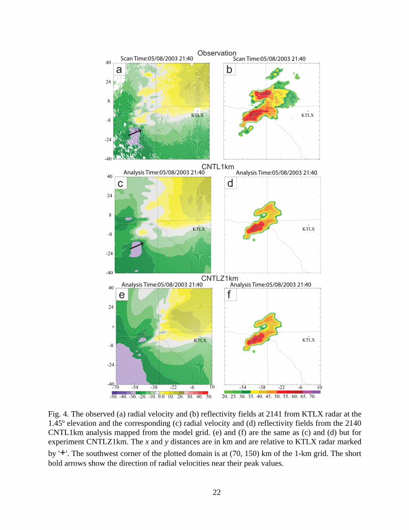
a) Results of data assimilation To directly compare the final analyses at 2140 with radar observations, Vr and Z values

simulated from the gridded analyses of CNTL1km and CNTLZ1km are mapped to the 1.45º elevation of the KTLX radar (Fig. 4). Here simple geometric mapping and spatial interpolation are done to simulate the observations in the radar coordinates. The beam pattern or reflectivity weighting for Vr simulation is not considered. The use of 1.45 rather than the lowest 0.5 elevation is done to avoid the effects of ground clutter. At the distance of the low-level rotation features from the radar, the 1.45 elevation is still fairly close the ground (~1.18 km AGL).

At the time of final analysis at 2140, the observed OKC storm is in its mature stage (Fig. 4a, 4b). The analyzed Vr and Z fields from CNTL1km show a general agreement with observations. The analyzed Vr field (Fig. 4c) faithfully reproduces the general pattern of observed Vr field (Fig. 4a), and clearly shows an inbound-outbound radial velocity couplet indicative of a mesocyclone near the southwestern tip of the reflectivity. The winds outside the mesocyclone are also well analyzed. The analyzed reflectivity field (Fig. 4d) is qualitatively similar to the observed field (Fig. 4b), exhibiting a hook echo in the main right-moving cell and a left-moving cell that is almost disconnected with the main cell. Note that by this time the observed Storm A (c.f. Fig. 1) has dissipated; the weak echo southeast of the hook echo is not associated with Storm A.

For comparison, the analyzed Vr and Z fields from experiment CNTLZ1km are plotted in Fig. 4e and 4f, respectively. When Vr data are not assimilated in CNTLZ1km, the analyzed Vr field (Fig. 4e) has a much poorer agreement with the observations (Fig. 4a). The mesocyclone rotation is essentially absent and the field is smoother. The analysis of Vr data helps capture the mesocyclone and improve the overall flow field. The corresponding Z field from CNTLZ1km (Fig. 4f) is very similar to that of CNTL1km (Fig. 4d) because of the direct assimilation of Z observations.

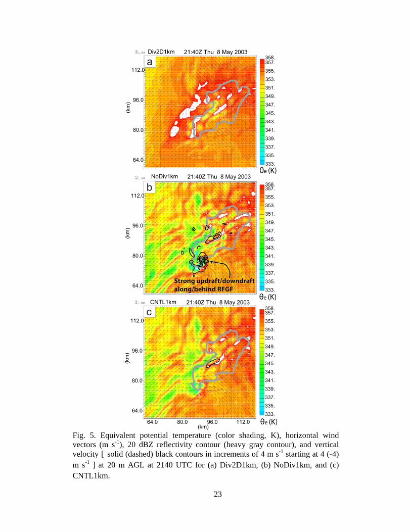
The analyzed Vr and Z fields from sensitivity experiments for divergence constraint, i.e., experiments Div2D1km and NoDiv1km, are not shown since they are very similar to those of CNTL1km, because Vr and Z observations are directly analyzed. In general, the role of the 2D divergence constraint is to couple together the two horizontal wind components, forcing them to adjust to each other so as to weakly satisfy the zero-divergence constraint. This actually has the side effect of weakening the updrafts and downdrafts in the analysis. Applying the divergence constraint in every assimilation cycle significantly reduces the intensity of vertical motion in the analyzed OKC supercell, weakening the overall storm. As such, at end of the assimilation window (i.e., at 2140) in Div2D1km, because of the much weaker downdraft, the low-level cold

7

pool associated with the storm is also much weaker (Fig. 5a). In contrast, the lack of the divergence constraint in NoDiv1km allows for the development of a much stronger surface cold pool as well as strong pockets of updraft and downdraft by 2140 (Fig. 5b). Not including any divergence constraint is undesirable since the 3DVAR will not be able to produce much of the cross-beam wind increment (Hu et al. 2006b). CNTL1km represents a compromise between full use and complete exclusion of the divergence constraint, by including the 2D divergence constraint in the final two analysis cycles only. The resulting analysis contains a well-established cold pool while the rotational signature in the hook region is also captured to some extent (Fig. 5c). The forecast model seems to be able to adequately establish updrafts and downdrafts during the subsequent forecast, as will be discussed later.

Another way to examine the quality of the analyzed wind fields is to compare them against independent radar radial velocity observations. Fortunately, for this case, data from the experimental WSR-88D radar at Norman Oklahoma (KOUN), and the Oklahoma TDWR radar (KOKC) are available (Romine et al. 2008). We compare the simulated radial velocity data at 2140, the end of the data assimilation window, from each of the four 1-km experiments, against the KOUN and KOKC observations. Specifically, we calculate the bias and root-mean squared error (RMSE) of the radial velocity differences at the 2.4 degree elevation angle for KOUN and the 2.5 degree elevation angle for KOKC, in a 20 km by 20 km area roughly centered on the observed radial velocity couplet that is about 25 km west of KOUN and 15 km west of KOKC. Such lower elevations are examined because they are the levels where the mesocyclone feature is most prominent. Without the assimilation of any radial velocity data, CNTLZ1km produces the worst fit of the wind analysis to independent radial velocity observations (Table 2). The three experiments that assimilated KTLX radial velocity data have comparable biases and RMSEs, although NoDiv1km has somewhat larger biases and errors compared to KOUN data while CNTL1km has the smallest RMSEs; suggesting a slightly better analysis of the mesocyclone region than in other experiments. In the following section, we will examine the forecasts resulting from the final analyses at 2140, which can further indicate the overall quality of the analysis.

b) Forecast results In this section we examine the forecasts starting from the final analyses at 2140 from the

1-km assimilation experiments. Given our primary interests in predicting tornadoes, we will emphasize low-level rotational features.

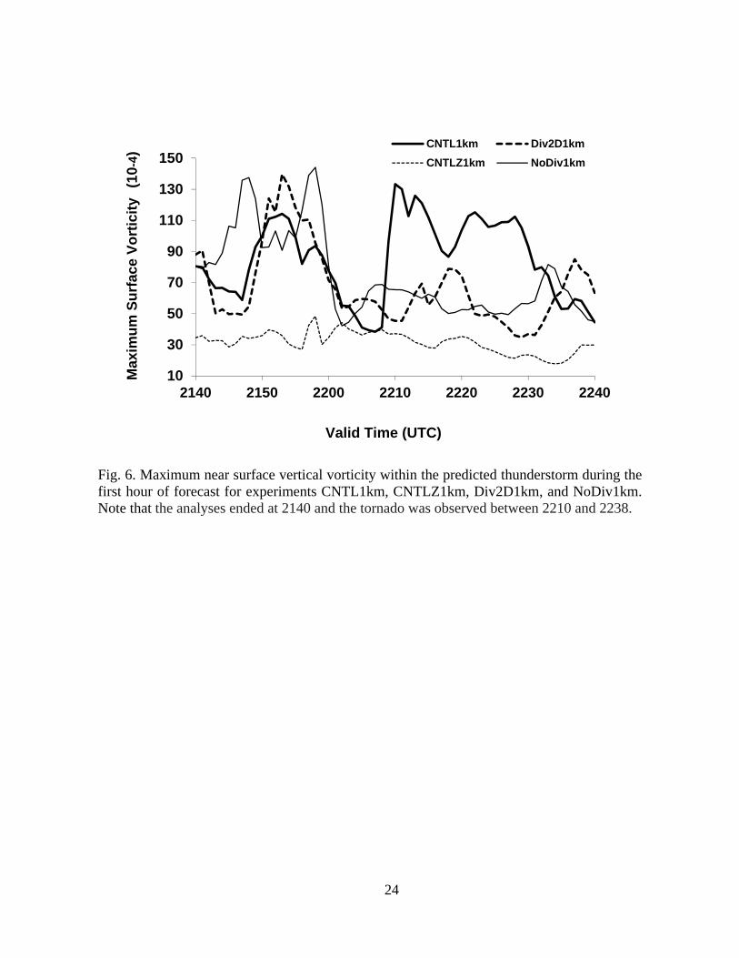
1) EVOLUTION OF VERTICAL VORTICITY NEAR THE SURFACE To examine the evolution of low-level rotation2 in the simulated supercell, we first plot in

Fig. 6 time series of predicted maximum vertical vorticity at the first model level of scalar variables above ground (~10 m AGL) for the four 1-km experiments. The time series from CNTL1km shows two periods of vorticity intensification, the first around 2150 and the second after 2205. The first period is well captured by all three experiments that assimilate Vr data.

2 Mid-level vorticity and vertical velocity were also examined (not shown). At mid-levels all experiments generally had comparably intense mid-level updrafts and mesocyclones, although the maximum vertical vorticity in CNTL1km in somewhat larger while that is NoDiv1km tends to be the smallest after 2205. This is likely reflective of the fact that all experiments produced supercellular structures with rotating updrafts. The main difference among the experiments was with the evolution of the low-level features.

8

During the second intensification period from 2205 to 2240, which spans the period of the observed OKC tornado, the maximum vorticity in CNTL1km increases rapidly from about 0.004 s-1 to a peak value of over 0.013 s-1 within ~2 minutes of 2210, and then stays mostly over 0.01 s-

1 for the next 20 minutes, while those of Div2D1km and NoDiv1km remain mostly below 0.006 s-1.

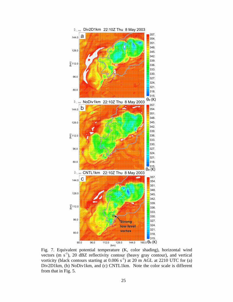
Experiments CNTL1km, Div2D1km and NoDiv1km differ only in the use of the divergence constraint. Because of nonlinear evolutions and interactions throughout the assimilation cycles, it is difficult to directly pinpoint the direct effect of the constraint. But as pointed out earlier, in Div2D1km that uses the 2D constraint throughout the cycles, the resulting storm and the associated cold pool (and associated gust frontal convergence) are weaker. The weaker cold pool in the rear-flank region of Div2D1km appears to preclude the development of strong low-level rotation in the forecast period (Fig. 7a). Meanwhile, in NoDiv1km, the portion of the cold pool just north of the reflectivity appendage (hook echo) is stronger and quickly spreads southeastward, preventing the development of a distinct rear-flank gust front (RFGF) and associated area of strong low-level rotation (Fig. 7b). In CNTL1km, strong low-level rotation develops in the forecast period along the rear-flank and forward-flank gust front occlusion point (Fig. 7c). Previous studies (e.g., Snook and Xue 2008; Markowski and Richardson 2009) have suggested that tornadogenesis may require just the right intensity of cold pool so that the low-level gust frontal convergence forcing is aligned with the mid-level mesocyclone-induced lifting.

In experiment CNTLZ1km, the maximum near surface vertical vorticity generally remains below 0.004 s-1, and there is no indication of any vortex intensification during the entire 1-hr period. This indicates the importance of assimilating Vr data in this case for capturing important circulation features that lead to low-level vortex intensification during the forecast. These results are consistent with the findings of Hu et al. (2006a; 2006b) who also found that assimilating Vr data in addition to Z observations helped produce stronger low-level rotation that better matched observations in a tornadic thunderstorm that they studied. In the following, we discuss the forecast fields during the second vorticity intensification period in more detail, through comparisons with radar observations.

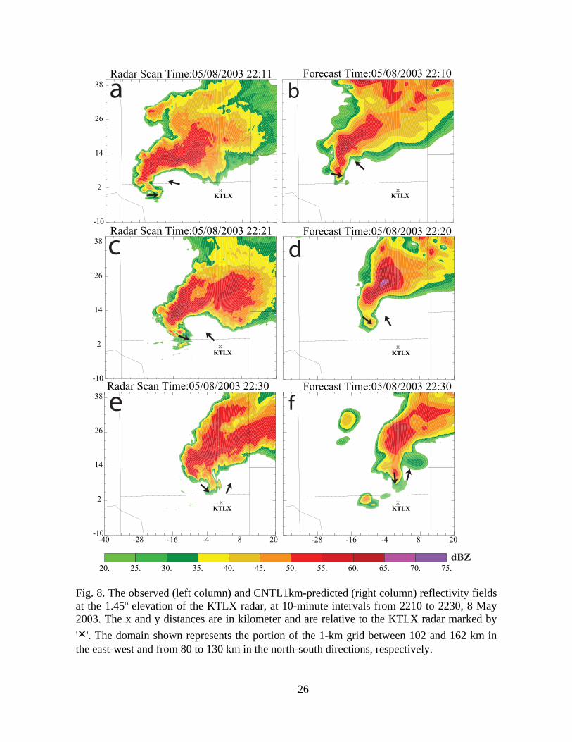
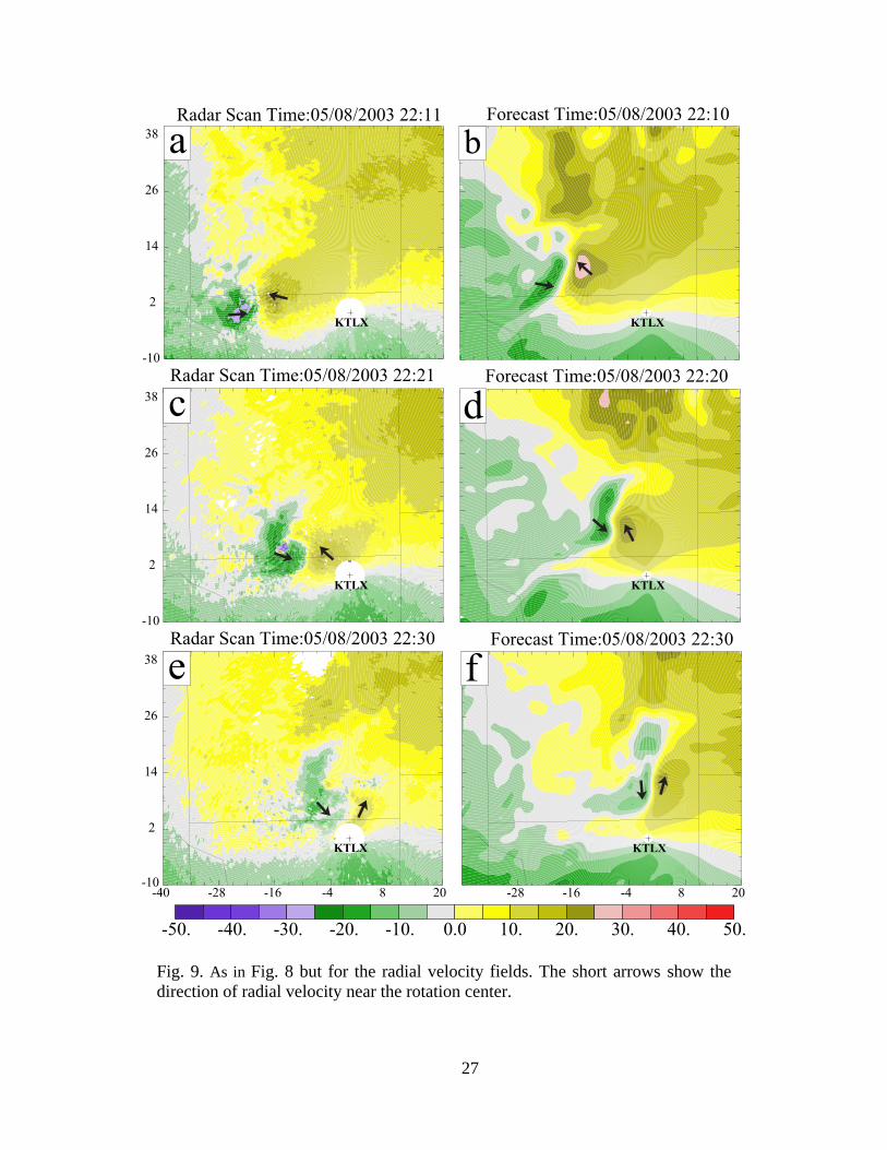
2) VERIFICATION OF FORECASTS IN RADAR OBSERVATION SPACE The observed and predicted Z and Vr fields at the 1.45º elevation of the KTLX radar are

plotted in Fig. 8 and Fig. 9, respectively, for CNTL1km, at 10 min intervals for the second vorticity intensification period from 2210 to 2230, corresponding to 40 to 60 minutes of free forecast in the experiment. The AGL height of the hook echo at 1.45 degree elevation is about 650 m at 2211, 390 m at 2221, and 300 m at 2230. These fields show that, as indicated by both the hook echo and Vr couplet patterns (Fig. 8a and c and Fig. 9a and c), the observed low-level rotation continues to intensify between 2211 and 2221. After 2221, the vortex begins to weaken, and by 2230, the hook echo was still evident but becomes less well defined and is associated with a weaker and smaller vorticity couplet (Fig. 8e and Fig. 9e). While some of the differences could be caused by the change in the radar range relative to the vortex, the weakening trend is clear. Throughout this period, the observed OKC storm moves east-northeastward. The forecast OKC storm in CNTL1km moves in the same direction and at a similar speed but is displaced northeastward by about 10 km throughout most of the period. During the data assimilation stage, hydrometeors derived from radar reflectivity observations were analyzed onto the model grid, ensuring a good match of the analyzed storm location with reflectivity observations. The rapid

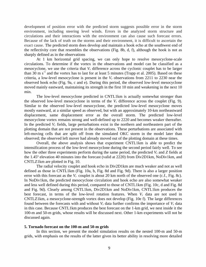
9

development of position error with the predicted storm suggests possible error in the storm environment, including steering level winds. Errors in the analyzed storm structure and circulations and their interactions with the environment can also cause such forecast errors. Because of the lack of truth on the storms and their environment, it is difficult to ascertain the exact cause. The predicted storm does develop and maintain a hook echo at the southwest end of the reflectivity core that resembles the observations (Fig. 8b, d, f), although the hook is not as sharply defined as in the observations

At 1 km horizontal grid spacing, we can only hope to resolve mesocyclone-scale circulations. To determine if the vortex in the observations and model can be classified as a mesocyclone, we use the criteria that Vr difference across the cyclonic couplet has to be larger than 30 m s-1 and the vortex has to last for at least 5 minutes (Trapp et al. 2005). Based on these criteria, a low-level mesocyclone is present in the Vr observations from 2211 to 2230 near the observed hook echo (Fig. 9a, c and e). During this period, the observed low-level mesocyclone moved mainly eastward, maintaining its strength in the first 10 min and weakening in the next 10 min.

The low-level mesocyclone predicted in CNTL1km is actually somewhat stronger than the observed low-level mesocyclone in terms of the Vr difference across the couplet (Fig. 9). Similar to the observed low-level mesocyclone, the predicted low-level mesocyclone moves mostly eastward, at a similar speed as observed, but with an approximately 10-km northeastward displacement, same displacement error as the overall storm. The predicted low-level mesocyclone vortex remains strong and well-defined up to 2220 and becomes weaker thereafter. In the predicted Vr fields, large perturbations exist in the northern and northeastern part of the plotting domain that are not present in the observations. These perturbations are associated with left-moving cells that are split off from the simulated OKC storm in the model later than observed; the observed left mover had already moved out of the plotting domain at these times.

Overall, the above analysis shows that experiment CNTL1km is able to predict the intensification process of the low-level mesocyclone during the second period fairly well. To see how the other three experiments perform during the same period, the predicted Vr and Z fields at the 1.45º elevation 40 minutes into the forecast (valid at 2220) from Div2D1km, NoDiv1km, and CNTLZ1km are plotted in Fig. 10.

The radial velocity couplet and hook echo in Div2D1km are much weaker and not as well defined as those in CNTL1km (Fig. 10a, b, Fig. 8d and Fig. 9d). There is also a larger position error with this forecast as the Vr couplet is about 20 km north of the observed one (c.f., Fig. 8c). In NoDiv1km, the predicted mesocyclone circulation and hook echo are also somewhat weaker and less well defined during this period, compared to those of CNTL1km (Fig. 10c, d and Fig. 8d and Fig. 9d). Clearly among CNTL1km, Div2D1km and NoDiv1km, CNTL1km produces the best forecast, in terms of the low-level rotation features. When Vr data are not used in CNTLZ1km, a mesocyclone-strength vortex does not develop (Fig. 10e f). The large differences found between the forecasts with and without Vr data further confirms the importance of Vr data in this case. Because CNTL1km produces the best forecast on the 1-km grid, we nest inside it the 100-m and 50-m grids, whose results will be discussed next. Other 1-km experiments will not be discussed again.

5. Tornado forecast on the 100-m and 50-m grids

In this section, we present the model simulation results on the nested 100-m and 50-m grids, with emphasis on the results of the latter given its better ability in resolving more detailed

10

tornadic structures. An important goal is to establish the physical credibility of the model simulated tornadoes by comparing with available observational information, so as to facilitate (separate) detailed diagnostic studies for the understanding of the tornadogenesis processes.

Fig. 2 shows the model-predicted tornado tracks, as defined by the surface vorticity maximum in the hook echo region of the storm, on both 100-m and 50-m grids, as compared to the observed tornado damage track. The plotted tracks show that the tornado developments in the two simulations are similar. In both simulations, a tornado forms around 2210, approximately 8 km north of the observed OKC tornadogenesis location. After reaching F-3 intensity on the 50-m grid (high-end F-2 intensity in the 100-m simulation) this tornado briefly weakens before re-intensifying. The tornadoes in the two simulations take a similar track, persist 13-14 min, and dissipate around 2225 at similar locations. The main difference between the two simulations is the development of a second, weaker and short-lived, tornado to the east of the first tornado in the 50-m simulation but not in the 100-m simulation. If the second tornado is considered the continuation of the first one in the 50-m simulation, its total length of the tornado track matches the observed one better than that of 100-m simulation. Given that and the fact that the 50-m grid is able to resolve more detailed structures, we will focus on the 50-m simulation in the remainder of this section. Still, the relative similarity between the two simulations suggests a certain degree of robustness of the simulations even at the tornado vortex scale.

a) Storm structure on the 50-m grid Before diving into the tornado-scale details, we first examine the storm-scale structures

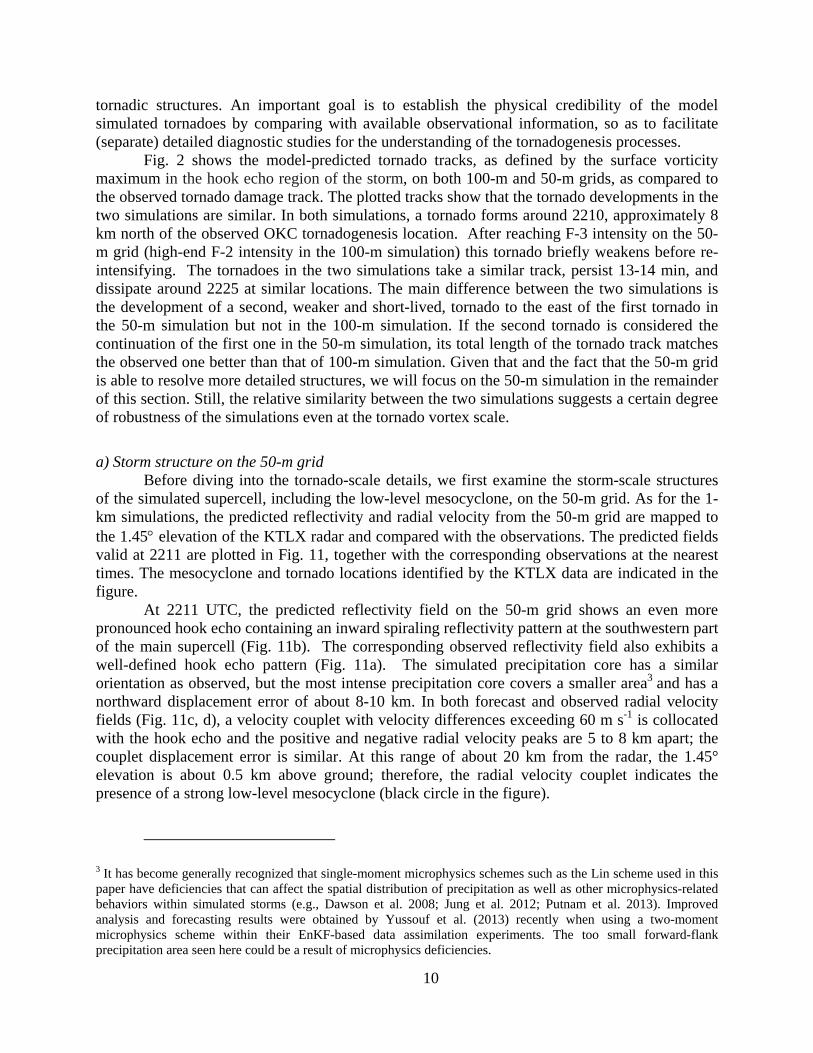
of the simulated supercell, including the low-level mesocyclone, on the 50-m grid. As for the 1-km simulations, the predicted reflectivity and radial velocity from the 50-m grid are mapped to the 1.45 elevation of the KTLX radar and compared with the observations. The predicted fields valid at 2211 are plotted in Fig. 11, together with the corresponding observations at the nearest times. The mesocyclone and tornado locations identified by the KTLX data are indicated in the figure.

At 2211 UTC, the predicted reflectivity field on the 50-m grid shows an even more pronounced hook echo containing an inward spiraling reflectivity pattern at the southwestern part of the main supercell (Fig. 11b). The corresponding observed reflectivity field also exhibits a well-defined hook echo pattern (Fig. 11a). The simulated precipitation core has a similar orientation as observed, but the most intense precipitation core covers a smaller area3 and has a northward displacement error of about 8-10 km. In both forecast and observed radial velocity fields (Fig. 11c, d), a velocity couplet with velocity differences exceeding 60 m s-1 is collocated with the hook echo and the positive and negative radial velocity peaks are 5 to 8 km apart; the couplet displacement error is similar. At this range of about 20 km from the radar, the 1.45° elevation is about 0.5 km above ground; therefore, the radial velocity couplet indicates the presence of a strong low-level mesocyclone (black circle in the figure).

3 It has become generally recognized that single-moment microphysics schemes such as the Lin scheme used in this paper have deficiencies that can affect the spatial distribution of precipitation as well as other microphysics-related behaviors within simulated storms (e.g., Dawson et al. 2008; Jung et al. 2012; Putnam et al. 2013). Improved analysis and forecasting results were obtained by Yussouf et al. (2013) recently when using a two-moment microphysics scheme within their EnKF-based data assimilation experiments. The too small forward-flank precipitation area seen here could be a result of microphysics deficiencies.

11

Compared to the 1-km forecast during the same period, the 50-m grid not only captures much finer scale structures of the hook echo and the associated circulation, but also improves the orientation of the precipitation echoes. The predicted precipitation area on the 50-m grid is aligned more in the east-west direction as observed (Fig. 11b) while the CNTL1km prediction has a much more north-south orientation (Fig. 8b). The predicted hook echo is also much better defined on the 50-m grid than on the 1-km grid in CNTL1km; the predicted radial velocity field contains more details than on the 1-km grid (Fig. 11d and Fig. 9b), and the couplet structure generally agrees with the observation better (Fig. 11c,d) and represents a stronger mesocyclone. In addition, a smaller-scale couplet with strong inbound and outbound radial velocity maxima are clearly visible in the simulation (red circle in Fig. 11d), which corresponds to the tornado vortex. This is less evident in the radar measurements (Fig. 11c), suggesting the observed tornado at this time may not be as large or as deep.

The corresponding low-level reflectivity and radial velocity fields at 2216 are shown in Fig. 12. As will be discussed in the next section (see Fig. 13), 2211 and 2216 are not at a time when the low-level vorticity reaches a maximum in the model; they are the times when the low-level scans of KTLX radar are available. Still, the low-level fields in the model at both times exhibit close resemblance to the obsevations. By 2216, the observed hook echo is even better developed, with an almost isolated reflectivity maximum forming (Fig. 12a) at the center of radial velocity couplet (Fig. 12c). Compared to 2211, the model simulated features have evolved somewhat but remain generally similar. As will be shown later, these two times correspond to the beginning of two vortex intensification phases, and the low-level vortex structures have some similarities. Of note is that the velocity couplet associated with the tornado vortex is evident in both observations and simulation, and they are similarly located relative to the mesocyclone.

b) The evolution of predicted tornadoes Time series of the maximum near-surface (about 10 m AGL) vertical vorticity, wind

speed, and minimum perturbation pressure from the 50-m forecast are plotted in Fig. 13. This figure shows that a small, short-lived vortex develops, strengthens, and dissipates all within the first 30 seconds of the simulation. A closer examination reveals that this vortex is located on the north side of the forward-flank downdraft (not shown) and does not correspond to any observed tornado. A stronger vortex then develops around 2209 UTC and reaches tornadic wind strength around 2211 UTC. Here, we consider a persistent vortex that lasts no shorter than 2 min and whose surface wind speed exceeds 32 m s -1 (the threshold of F1 intensity tornado) a tornado. The simulated tornado quickly intensifies and reaches wind speeds associated with high-end F-3 tornadoes at 2214 UTC, with maximum wind speeds exceeding 85 m s-1 and a 45 hPa pressure drop corresponding to a maximum vertical vorticity of over 1.5 s-1

at 10 m AGL. The tornado then weakens to F-1 intensity from 2215 to 2217 before re-intensifying to high-end F-2 intensity from 2218 to 2224. The tornado rapidly dissipates afterwards.

Concurrent with the re-intensification of the first tornado, a second tornado formed around 2220 about 5 km east of the first tornado. This tornado is much smaller and somewhat weaker than the first tornado. Because the tornadoes are concurrent, it is not possible to distinguish them from the time-series plot in Fig. 13. However, examination of the wind fields (not shown) reveals that, in terms of wind speed, the first tornado is the stronger of the two until 2224 and is responsible for the >60 m s-1 wind speed plotted in Fig. 13. The second tornado has maximum wind speeds of around 50 m s-1. It is noted that owing to its small size, the second tornado is associated with the maximum vorticity values plotted in Fig. 13 after 2220.

12

As discussed earlier, the simulated tornado paths (diagnosed by tracking the circulation center of the predicted tornadoes) on the 50-m and 100-m grids are plotted in Fig. 2 along with the observed tornado damage path. The simulated tornadoes on both the 100-m and 50-m simulations are both shorter-lived and weaker than the observed OKC tornado. In addition, the simulated tornado paths are approximately 8 km north of the observed track. Despite these, the timing of the tornadogenesis at 2211 UTC in the 100-m and 50-m forecasts agrees well with the timing of observed tornadogenesis, which occurred at around 2210 UTC. Additionally, the track orientation agrees well with the observed tornado track. The northward displacement of the tornado track appears to be more due to the northward displacement of the overall storm (see Fig. 8) than due to the relative position of the tornado within the storm. Given that tornadoes are generally very difficult to predict, in terms of both timing and position, or even the occurrence at all, we consider the model prediction rather encouraging; we are not aware of predictions of similar quality in the published literature so far. The similarity between the timings and storm-relative locations of the simulated and observed tornadoes provides additional evidence that the two correspond to the same object, i.e., that the simulated tornado results from a similar dynamical pathway as the observed tornado. An examination of the tornado structures in the following section also indicates realism of the simulated tornado.

c) Detailed structure of predicted tornadoes on the 50-m grid We have shown that the 50-m grid spacing simulation produced a strong tornado that

tracked within 8 km of the observed OKC tornado. To further justify the claim that the model-simulated tornadoes are realistic, we examine in more detail the low-level fields associated with the simulated tornadoes, and link the simulated features with tornado conceptual models from previous studies.

Fig. 14 presents the time evolution of the near-surface vertical vorticity associated with the first tornado in the 50-m simulation. This figure shows that the tornado initially has a single-cell structure when the maximum vertical vorticity is found at the vortex center; it quickly evolves into a structure with a maximum vorticity ring by 2212 then breaks down into multiple vortices that develop on the vorticity ring between 2213 and 2215. The tornado during this period is characteristic of a vortex with very large values of swirl ratio (e.g., Davies-Jones 1986; 2001). After 2215, the tornado weakens with a large area of less organized vorticity. Around 2217, the tornado re-intensifies and the high vorticity becomes more concentrated; after 2219 the tornado takes on a classic two-celled (Davies-Jones 1986; Davies-Jones et al. 2001) appearance with a well-formed ring of vorticity surrounding a central downdraft. This structure is also indicative of fairly large values of swirl ratio, though likely not as large as those at the earlier times when sub-vortices were much better defined.

To further examine the structure of the simulated tornado, Fig. 15 presents horizontal and vertical cross sections of velocity and vorticity fields associated with the first simulated tornado at 2213 and 2220, the times when the tornado’s low-level vertical vorticity is near its peak values (Fig. 13). At 2213, at the first model above surface or about 10 m AGL (Fig. 15a), an arc of large positive vertical vorticity and upward vertical velocity is present, that contains intense subvortices rotating cyclonically around the tornado vortex. The maximum winds associated with the simulated tornado are found within these subvortices. Near the center of the vortex is downward motion. A south-north vertical cross-section through the tornado (and strongest subvortex) at this time (Fig. 15c) reveals that the northern part of the tornado is predominantly characterized by strong updrafts that extend above 1.5 km height. The strongest low-level

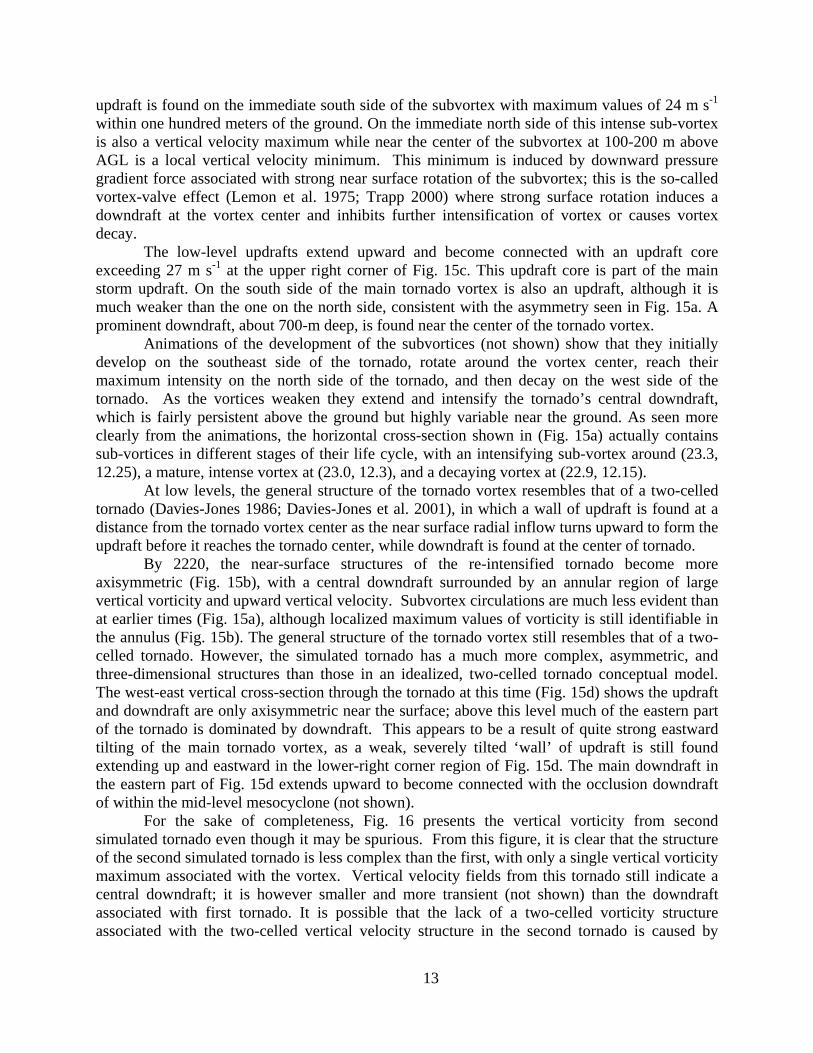
13

updraft is found on the immediate south side of the subvortex with maximum values of 24 m s-1 within one hundred meters of the ground. On the immediate north side of this intense sub-vortex is also a vertical velocity maximum while near the center of the subvortex at 100-200 m above AGL is a local vertical velocity minimum. This minimum is induced by downward pressure gradient force associated with strong near surface rotation of the subvortex; this is the so-called vortex-valve effect (Lemon et al. 1975; Trapp 2000) where strong surface rotation induces a downdraft at the vortex center and inhibits further intensification of vortex or causes vortex decay.

The low-level updrafts extend upward and become connected with an updraft core exceeding 27 m s-1 at the upper right corner of Fig. 15c. This updraft core is part of the main storm updraft. On the south side of the main tornado vortex is also an updraft, although it is much weaker than the one on the north side, consistent with the asymmetry seen in Fig. 15a. A prominent downdraft, about 700-m deep, is found near the center of the tornado vortex.

Animations of the development of the subvortices (not shown) show that they initially develop on the southeast side of the tornado, rotate around the vortex center, reach their maximum intensity on the north side of the tornado, and then decay on the west side of the tornado. As the vortices weaken they extend and intensify the tornado’s central downdraft, which is fairly persistent above the ground but highly variable near the ground. As seen more clearly from the animations, the horizontal cross-section shown in (Fig. 15a) actually contains sub-vortices in different stages of their life cycle, with an intensifying sub-vortex around (23.3, 12.25), a mature, intense vortex at (23.0, 12.3), and a decaying vortex at (22.9, 12.15).

At low levels, the general structure of the tornado vortex resembles that of a two-celled tornado (Davies-Jones 1986; Davies-Jones et al. 2001), in which a wall of updraft is found at a distance from the tornado vortex center as the near surface radial inflow turns upward to form the updraft before it reaches the tornado center, while downdraft is found at the center of tornado.

By 2220, the near-surface structures of the re-intensified tornado become more axisymmetric (Fig. 15b), with a central downdraft surrounded by an annular region of large vertical vorticity and upward vertical velocity. Subvortex circulations are much less evident than at earlier times (Fig. 15a), although localized maximum values of vorticity is still identifiable in the annulus (Fig. 15b). The general structure of the tornado vortex still resembles that of a two-celled tornado. However, the simulated tornado has a much more complex, asymmetric, and three-dimensional structures than those in an idealized, two-celled tornado conceptual model. The west-east vertical cross-section through the tornado at this time (Fig. 15d) shows the updraft and downdraft are only axisymmetric near the surface; above this level much of the eastern part of the tornado is dominated by downdraft. This appears to be a result of quite strong eastward tilting of the main tornado vortex, as a weak, severely tilted ‘wall’ of updraft is still found extending up and eastward in the lower-right corner region of Fig. 15d. The main downdraft in the eastern part of Fig. 15d extends upward to become connected with the occlusion downdraft of within the mid-level mesocyclone (not shown).

For the sake of completeness, Fig. 16 presents the vertical vorticity from second simulated tornado even though it may be spurious. From this figure, it is clear that the structure of the second simulated tornado is less complex than the first, with only a single vertical vorticity maximum associated with the vortex. Vertical velocity fields from this tornado still indicate a central downdraft; it is however smaller and more transient (not shown) than the downdraft associated with first tornado. It is possible that the lack of a two-celled vorticity structure associated with the two-celled vertical velocity structure in the second tornado is caused by

14

insufficient model resolution as the second tornado is only ~200-m in diameter, with the central downdraft only present in at most a couple of model grid points. It is also possibly because that this vortex is weaker and has a small swirl ratio.

Overall, although (not surprisingly) being much more complex owing to the multi-scale interactions inherent in a realistic three-dimensional simulation of a tornadic supercell, the structures seen in the simulated tornadoes are similar to those that have been observed in tornado chambers (Church et al. 1979; Rotunno 1979), discussed theoretically (Snow 1978; Davies-Jones 1986; Davies-Jones et al. 2001), simulated via large-eddy simulations (e.g., Lewellen et al. 1997), and more recently observed by high-resolution mobile Doppler radars (Wurman 2002; Bluestein et al. 2003; Alexander and Wurman 2005; Lee and Wurman 2005; Kosiba and Wurman 2010). These similarities lend credence to the assertion that the intense vortices in the high-resolution simulation are realistic representations of actual tornadoes. This finding is encouraging as it indicates that the eventual model-based prediction of tornadoes may be possible in real-time (given adequate computational resources), which is an essential goal of warn-on-forecast (Stensrud et al. 2009). The direct comparison with available radar observations of the simulated low-level flow and precipitation structures associated with the low-level mesocyclone, and the reasonable timing, location and structure of the simulated tornadoes suggest that they are sufficiently ‘real’ to warrant a detailed dynamical analysis of the tornadogenesis processes with this case. This will be the focus of a separate paper (Schenkman et al. 2013).

6. Summary and discussion

In this study, the 8 May 2003 Oklahoma City tornadic supercell and embedded tornadoes are predicted using the ARPS model, starting from an initial condition that assimilated Doppler radar as well as conventional observations. The prediction uses four one-way nested grids to reach tornado-resolving horizontal resolutions of 50 m with high-frequency radar data assimilation performed on the 1-km grid.

Specifically, hourly cycles assimilating conventional data are first performed using the ARPS 3DVAR on the outermost 9-km grid which provides the background for the initial analysis on the 1-km grid as well as the lateral boundary conditions. Data assimilation cycles at 5 minute intervals are then performed on the 1-km grid over a 70 minute window that covers the developmental stages of the 8 May 2003 OKC supercell. In each analysis, radar radial velocity data are analyzed through the ARPS 3DVAR and reflectivity data are analyzed by the ARPS complex cloud analysis. The latter analyzes microphysical fields and adjusts in-cloud temperature and moisture. Four 1-km experiments are conducted to study the impacts of radar data and a divergence constraint in the 3DVAR. The predictions on the 1-km grid are verified directly against radar observations in terms of the radial velocity Vr and reflectivity Z mapped to a lower elevation of OKC operational Doppler radar.

The assimilation of both Vr and Z data, while imposing a 2D divergence constraint within the last two analysis cycles, is shown to successfully analyze the low-level mesocyclone. Comparison of the analyzed radial velocity against independent observations from two other radars suggests best analysis quality in the low-level mesocyclone region is obtained with this experiment design. This experiment also produces the best forecast during the tornadic phase of the storm on the 1-km grid; it successfully reproduces the observed development and propagation of the mesocyclone and associated echo pattern between 30 to 50 minutes of forecast; with the main error being with the location of the predicted system that is about 8 km too far to the north.

15

Two other 1-km experiments that differ in the use of the 2D divergence constraint predict mesocyclones and hook echo patterns that are weaker and less well defined than observations. Another experiment that assimilated only reflectivity data on the 1-km grid failed to properly analyze or predict almost all pertinent features associated with the tornadic supercell. Even though the application of the 2D divergence constraint within the final two assimilation cycles produced the best results in this case, the general behavior and impacts of divergence constraint within the 3DVAR on storm analysis still requires further investigation.

Given the rather realistic 1-km forecast of the tornadic supercell, two grids with 100-m and 50-m grid spacings were successively nested within the control 1-km forecast. The 100-m grid was started at the same time as the 1-km forecast while the 50-m grid started from interpolated 20-minute forecast of the 100-m grid. Both experiments successfully predicted the intensification of low-level vortices that reached tornadic intensity, reaching F-2 intensity on the 100-m grid and high-end F-3 on the 50-m grid. Although the predicted tornadoes were shorter-lived than the actual tornado, they formed in the model within the same time period of the actual tornado and traveled along a path that is parallel to, though about 8 km north of, the observed tornado damage track.

Even though the 100-m and 50-m grid forecasts were started at different times, they both produced a tornado strength vortex at similar location and time. The consistency between the two high-resolution forecasts indicates that the forecast tornado-strength vortex is likely a predictable feature and not an artifact of resolution increase. Otherwise, we would expect the 100-m tornado to occur much sooner.

Examination of the near-surface flow fields of the simulated tornadoes showed that the forecast contained many features that are consistent with those of theoretical, laboratory, and observational studies of tornadoes. The 50-m grid apparently has enough resolution to resolve two-celled tornado vortices that contain a maximum vorticity vortex ring surrounding the vortex center of lower vorticity and downward motion, and sub-vortices develop along the vortex ring. These sub-vortices were associated with the maximum winds in the simulated tornado, and likely correspond to the ‘suction vortices’ documented in the literature (e.g., Fujita et al. 1976).

Overall, the high-resolution experiments conducted in this study demonstrates that it is possible to predict a realistic tornadic vortex tens of minutes ahead of the actual tornadogenesis, within 10 km of observed location using an state-of-the-art storm-scale numerical weather prediction model that assimilates high-frequency operational Doppler radar data. Such results are encouraging in the pursuit of a warn-on-forecast type system aiming at numerically predicting tornadoes with much longer lead times and spatial accuracy than typical extrapolation-based nowcasting techniques can offer. The reasonable forecasting results on the 1-km and finer tornado-resolving grids based on the low-cost 3DVAR data assimilation method are particularly encouraging from the operational point of view. At the same time, some special treatments had to be made in the experiments to obtain the desirable forecasting results, which are partly due to limitations of the assimilation method used and in the observation coverage (in terms of both space and state variables). Therefore, additional studies of other tornadic storm cases are necessary to better understand the predictability aspects of the tornado prediction science as well as the generality of the conclusions drawn in this paper. Given the highly nonlinear nature and the very short time scales of the tornado development and evolution, it will also be essential to estimate and quantify the prediction uncertainties; for that ensemble-based data assimilation and prediction would be an effective approach; in fact, probabilistic forecasting via ensembles is another key element of the warn-on-forecast concept (Stensrud et al. 2009). Stensrud et al. (2013)

16

provided examples on probabilistic forecasting of tornadic thunderstorms while Snook et al. (2012) demonstrated the efficacy of probabilistic prediction of tornadoes within a mesoscale convective system with up to three hours of lead time. Still, being able to numerically predict observed tornadoes with sufficient realism is a pre-requisite for explicit prediction of tornadoes in real time, whether it is a deterministic or probabilistic prediction system. The current study represents one of the initial steps towards examining and demonstrating such capabilities. Studies with more cases, and using more advanced data assimilation techniques and prediction models are certainly still needed.

Acknowledgement: This work was primarily supported by NSF grant AGS-0802888. The first author was also supported by NSF grants EEC-0313747, OCI-0905040, AGS-0750790, AGS-0941491, AGS-1046171, and AGS-1046081. Numerical simulations were performed at the University of Oklahoma Supercomputing Center for Education and Research (OSCER) and on an national XSEDE supercomputer at the National Institute of Computational Science (NICS) at the University of Tennessee. References Adlerman, E. J. and K. K. Droegemeier, 2002: The sensitivity of numerically simulated cyclic

mesocyclongenesis to variations in model physical and computational parameters. Mon. Wea. Rev., 130, 2671-2691.

Alexander, C. R. and J. Wurman, 2005: The 30 May 1998 Spencer, South Dakota, storm. Part I: The structural evolution and environment of the tornadoes. Mon. Wea. Rev., 133, 72-96.

Bluestein, H. B., et al., 2003: Mobile Doppler radar observations of a tornado in a supercell near Bassett, Nebraska, on 5 June 1999. Part II: Tornado-vortex structure. Mon. Wea. Rev., 131, 2968-2984.

Church, C. R., J. T. Snow, G. L. Baker, and E. M. Agee, 1979: Characteristics of Tornado-Like Vortices as a Function of Swirl Ratio - Laboratory Investigation. J. Atmos. Sci., 36, 1755-1776.

Davies-Jones, R., R. J. Trapp, and H. B. Bluestein, 2001: Tornadoes and tornadic storms. Severe Convective Storms, C. A. Doswell, III, Ed., Amer. Meteor. Soc., 167-222.

Davies-Jones, R. P., 1986: Tornado dynamics. Thunderstorm Morphology and Dynamics, E. Kessler, Ed., University of Oklahoma Press, 197-236.

Dawson, D. T., II, L. J. Wicker, E. R. Mansell, and R. L. Tanamachi, 2012: Impact of the environmental low-level wind profile on ensemble forecasts of the 4 May 2007 Greensburg, Kansas, tornadic storm and associated mesocyclones. Mon. Wea. Rev., 140, 696-716.

Dawson, D. T., II, M. Xue, J. A. Milbrandt, and M. K. Yau, 2008: Improvements in the treatment of evaporation and melting in multi-moment versus single-moment bulk microphysics: results from numerical simulations of the 3 May 1999 Oklahoma tornadic storms. 24th Conf. Severe Local Storms, Savannah, GA, Amer. Meteor. Soc., Paper 17B.4.

Dowell, D., et al., 2004: Wind and temperature retrievals in the 17 May 1981 Arcadia, Oklahoma supercell: Ensemble Kalman filter experiments. Mon. Wea. Rev., 132, 1982-2005.

Fujita, T. T., G. S. Forbes, and T. A. Umenhofer, 1976: Closeup view of 20 March 1976 tornadoes: Sinking cloud tops to suction vortices. Weatherwise, 29, 116-131.

17

Gao, J.-D., M. Xue, K. Brewster, and K. K. Droegemeier, 2004: A three-dimensional variational data analysis method with recursive filter for Doppler radars. J. Atmos. Ocean. Technol., 21, 457-469.

Hu, M. and M. Xue, 2007: Impact of configurations of rapid intermittent assimilation of WSR-88D radar data for the 8 May 2003 Oklahoma City tornadic thunderstorm case. Mon. Wea. Rev., 135, 507–525.

Hu, M., M. Xue, and K. Brewster, 2006a: 3DVAR and cloud analysis with WSR-88D level-II data for the prediction of Fort Worth tornadic thunderstorms. Part I: Cloud analysis and its impact. Mon. Wea. Rev., 134, 675-698.

Hu, M., M. Xue, J. Gao, and K. Brewster, 2006b: 3DVAR and cloud analysis with WSR-88D level-II data for the prediction of Fort Worth tornadic thunderstorms. Part II: Impact of radial velocity analysis via 3DVAR. Mon. Wea. Rev., 134, 699-721.

Jung, Y., M. Xue, and M. Tong, 2012: Ensemble Kalman filter analyses of the 29-30 May 2004 Oklahoma tornadic thunderstorm using one- and two-moment bulk microphysics schemes, with verification against polarimetric data. Mon. Wea. Rev., 140, 1457-1475.

Kosiba, K. and J. Wurman, 2010: The Three-Dimensional Axisymmetric Wind Field Structure of the Spencer, South Dakota, 1998 Tornado. J. Atmos. Sci., 67, 3074-3083.

Lee, W. C. and J. Wurman, 2005: Diagnosed three-dimensional axisymmetric structure of the Mulhall Tornado on 3 May 1999. J. Atmos. Sci., 62, 2373-2393.

Lemon, L. R., D. W. Burgess, and R. A. Brown, 1975: Tornado production and storm sustenance. Preprints, Ninth Conf. Severe Local Storms, Norman, OK, Amer. Meteor. Soc., 100–104.

Lewellen, W. S., D. C. Lewellen, and R. I. Sykes, 1997: Large-Eddy Simulation of a Tornado's Interaction with the Surface. J. Atmos. Sci., 54, 581-605.

Lin, Y.-L., R. D. Farley, and H. D. Orville, 1983: Bulk parameterization of the snow field in a cloud model. J. Climat. Appl. Meteor., 22, 1065-1092.

Markowski, P. M., et al., 2011: Characteristics of the wind field in a trio of nontornadic low-level mesocyclones observed by the doppler on wheels radars. Electronic J. Severe Storms Meteor., 6, 1-48.

Markowski, P. M. and Y. Richardson, 2009: Tornadogenesis: Our current understanding, forecasting considerations, and questions to guide future research. Atmos. Res., 93, 3-10.

Mashiko, W., H. Niino, and K. Teruyuki, 2009: Numerical simulations of tornadogenesis in an outer-rainband minisupercell of typhoon Shanshan on 17 September 2006. Mon. Wea. Rev., 137, 4238-4260.

Natenberg, E., J. Gao, M. Xue, and F. H. Carr, 2013: Multi-Doppler radar analysis and forecast of a tornadic thunderstorm using a 3D variational data assimilation technique and ARPS model. Adv. Meteor., Conditionally accepted.

Putnam, B. J., et al., 2013: The analysis and prediction of microphysical states and polarimetric variables in a mesoscale convective system using double-moment microphysics, multi-network radar data, and the ensemble Kalman filter. Mon. Wea. Rev., Accepted.

Romine, G. S., D. W. Burgess, and R. B. Wilhelmson, 2008: A dual-polarization-radar-based assessment of the 8 May 2003 Oklahoma City area tornadic supercell. Mon. Wea. Rev., 136, 2849-2870.

Rotunno, R., 1979: A study in tornado-like vortex dynamics. J. Atmos. Sci., 36, 140-155. Schenkman, A., M. Xue, and M. Hu, 2013: Tornadogenesis in a high-resolution simulation of the

8 May 2003 Oklahoma City supercell. J. Atmos. Sci., To be submitted.

18

Schenkman, A., et al., 2011: Impact of CASA radar and Oklahoma mesonet data assimilation on the analysis and prediction of tornadic mesovortices in a MCS. Mon. Wea. Rev., 139, 3422-3445.

Schenkman, A. D., M. Xue, and A. Shapiro, 2012: Tornadogenesis in a simulated mesovortex within a mesoscale convective system. J. Atmos. Sci., 69, 3372-3390.

Snook, N. and M. Xue, 2008: Effects of microphysical drop size distribution on tornadogenesis in supercell thunderstorms. Geophy. Res. Letters, 35, L24803, doi:10.1029/2008GL035866.

Snook, N., M. Xue, and Y. Jung, 2012: Ensemble probabilistic forecasts of a tornadic mesoscale convective system from ensemble Kalman filter analyses using WSR-88D and CASA radar data. Mon. Wea. Rev., 140, 2126-2146.

Snow, J. T., 1978: Inertial Instability as Related to Multiple-Vortex Phenomenon. J. Atmos. Sci., 35, 1660-1677.

Stensrud, D. J., et al., 2013: Progress and challenges with Warn-on-Forecast. Atmos. Res., 123, 2-16.

Stensrud, D. J., et al., 2009: Convective-scale Warn on Forecast System: A Vision for 2020. Bull. Am. Meteor. Soc., 90, 1487-1499.

Sun, J., et al., 2013: Use of NWP for nowcasting precipitation: Recent progress and challenges. Bull. Amer. Meteor. Soc., Accepted.

Tanamachi, R. L., et al., 2013: EnKF assimilation of high-resolution, mobile Doppler radar data of the 4 May 2007 Greensburg, Kansas, supercell into a numerical cloud model. Mon. Wea. Rev., 141, 625-648.

Trapp, R. J., 1999: Observations of nontornadic low-level mesocyclones and attendant tornadogenesis failure during VORTEX. Mon. Wea. Rev., 127, 1693-1705.

Trapp, R. J., 2000: A clarification of vortex breakdown and tornadogenesis. Mon. Wea. Rev., 128, 888-895.

Trapp, R. J., S. A. Tessendorf, E. S. Godfrey, and H. E. Brooks, 2005: Tornadoes from squall lines and bow echoes. Part I: Climatological distribution. Wea. Forecasting, 20, 23-34.

Wicker, L. J. and R. B. Wilhelmson, 1995: Simulation and analysis of tornado development and decay within a three-dimensional supercell thunderstorm. J. Atmos. Sci., 52, 2675-2703.

Wurman, J., 2002: The Multiple-Vortex Structure of a Tornado. Wea. Forecasting, 17, 473-505. Xue, M., K. K. Droegemeier, and D. Weber, 2007: Numerical prediction of high-impact local

weather: A driver for petascale computing. Petascale Computing: Algorithms and Applications, Taylor & Francis Group, LLC, 103-124.

Xue, M., K. K. Droegemeier, and V. Wong, 2000: The Advanced Regional Prediction System (ARPS) - A multiscale nonhydrostatic atmospheric simulation and prediction tool. Part I: Model dynamics and verification. Meteor. Atmos. Phy., 75, 161-193.

Xue, M., et al., 2001: The Advanced Regional Prediction System (ARPS) - A multi-scale nonhydrostatic atmospheric simulation and prediction tool. Part II: Model physics and applications. Meteor. Atmos. Phys., 76, 143-165.

Xue, M., et al., 2003: The Advanced Regional Prediction System (ARPS), storm-scale numerical weather prediction and data assimilation. Meteor. Atmos. Phy., 82, 139-170.

Yussouf, N., et al., 2013: The ensemble Kalman filter analyses and forecasts of the 8 May 2003 Oklahoma City tornadic supercell storm using single and double moment microphysics schemes, In press.

19

Fig. 1. Regions of radar echoes exceeding 35 dBZ as observed by KTLX radar at the 1.45º elevation. The echoes are at 30-minute intervals from 2101 to 2359, 8 May 2003. The grayscales of the echoes at two consecutive times are different, so are their outlines. The locations of the maximum reflectivity of the main storm are marked by + signs, together with the corresponding times. The x and y coordinates are in kilometer and have their origin at the KTLX radar site that is marked by . The arrow lines are the paths of the OKC storm and storms A, B, and C. Also, the hook echo at 2201 and Moore are pointed to by curved arrows. The Oklahoma County is highlighted (from Hu and Xue 2007).

-100 -60 -20 20 60 100-80

-40

0

40

80

2052

2101

2131

22012230

23002330

2359

KTLX

22302101

2201

Hook echo Moore

20

Fig. 2. The observed damage path of the 8 May OKC tornado (solid gray line) and the path of the modeled tornado on the 100-m grid (dashed gray line) and 50-m grid (solid black line), as represented by the central location of the tornado circulation. The life span of each tornado is also indicated by the time at the beginning and end of the path. The domain shown is 30 km 20 km in size.

21

Fig. 3. The nested domains of 9 km, 1 km, 100 m, and 50 m horizontal grid spacings (upper panel) and the timeline of the analyses and forecasts on each of the four grids (lower panel).

0 100 200 300 400 5000

100

200

300

400

500

(km)

(km

)

1/16 of 9 km grid

1 km grid

22

Fig. 4. The observed (a) radial velocity and (b) reflectivity fields at 2141 from KTLX radar at the 1.45º elevation and the corresponding (c) radial velocity and (d) reflectivity fields from the 2140 CNTL1km analysis mapped from the model grid. (e) and (f) are the same as (c) and (d) but for experiment CNTLZ1km. The x and y distances are in km and are relative to KTLX radar marked

by '+'. The southwest corner of the plotted domain is at (70, 150) km of the 1-km grid. The short bold arrows show the direction of radial velocities near their peak values.

-40

-24

-8

8

24

40

KTLX

-40

-24

-8

8

24

40

KTLX

-70 -54 -38 -22 -6 10-40

-24

-8

8

24

40

-50. -40. -30. -20. -10. 0.0 10. 20. 30. 40. 50.

KTLX

KTLX

20. 25. 30. 35. 40. 45. 50. 55. 60. 65. 70.

KTLX

Analysis Time:05/08/2003 21:40

Analysis Time:05/08/2003 21:40 Analysis Time:05/08/2003 21:40

Analysis Time:05/08/2003 21:40

Scan Time:05/08/2003 21:40 Scan Time:05/08/2003 21:40Observation

CNTL1km

CNTLZ1km

a b

dc

e

-54 -38 -22 -6 10

KTLX

f

23

Fig. 5. Equivalent potential temperature (color shading, K), horizontal wind vectors (m s-1), 20 dBZ reflectivity contour (heavy gray contour), and vertical velocity [ solid (dashed) black contours in increments of 4 m s-1 starting at 4 (-4) m s-1 ] at 20 m AGL at 2140 UTC for (a) Div2D1km, (b) NoDiv1km, and (c) CNTL1km.

333.

335.

337.

339.

341.

343.

345.

347.

349.

351.

353.

355.

357.358.

64.0

80.0

96.0

112.0

(km

)

Div2D1km 21:40Z Thu 8 May 2003

NoDiv1km 21:40Z Thu 8 May 2003

CNTL1km 21:40Z Thu 8 May 2003

5.05.0

333.

335.

337.

339.

341.

343.

345.

347.

349.

351.

353.

355.

357.358.

64.0

80.0

96.0

112.0

(km

)

5.05.0

333.

335.

337.

339.

341.

343.

345.

347.

349.

351.

353.

355.

357.358.

64.0 80.0 96.0 112.0

64.0

80.0

96.0

112.0

(km)

(km

)

5.05.0

θe (K)

θe (K)

θe (K)

a

b

c

Strong updraft/downdraft Strong updraft/downdraft along/behind RFGFalong/behind RFGF

24

Fig. 6. Maximum near surface vertical vorticity within the predicted thunderstorm during the first hour of forecast for experiments CNTL1km, CNTLZ1km, Div2D1km, and NoDiv1km. Note that the analyses ended at 2140 and the tornado was observed between 2210 and 2238.

10

30

50

70

90

110

130

150

2140 2150 2200 2210 2220 2230 2240

CNTL1km Div2D1km

CNTLZ1km NoDiv1km

Max

imu

m S

urf

ace

Vo

rtic

ity

Valid Time (UTC)

(10-

4)

25

Fig. 7. Equivalent potential temperature (K, color shading), horizontal wind vectors (m s-1), 20 dBZ reflectivity contour (heavy gray contour), and vertical vorticity (black contours starting at 0.006 s-1) at 20 m AGL at 2210 UTC for (a) Div2D1km, (b) NoDiv1km, and (c) CNTL1km. Note the color scale is different from that in Fig. 5.

315.318.321.324.327.330.333.336.339.342.345.348.351.354.357.

80.0

96.0

112.0

128.0

144.0

(km

)

10.010.0

Strong Strong low-level low-level vortexvortex

315.318.321.324.327.330.333.336.339.342.345.348.351.354.357.

80.0

96.0

112.0

128.0

144.0

(km

)

10.010.0

315.318.321.324.327.330.333.336.339.342.345.348.351.354.357.

80.0 96.0 112.0 128.0 144.0 160.0

80.0

96.0

112.0

128.0

144.0

(km)

(km

)

10.010.0

CNTL1km 22:10Z Thu 8 May 2003

Div2D1km 22:10Z Thu 8 May 2003

NoDiv1km 22:10Z Thu 8 May 2003

θe (K)

θe (K)

θe (K)

c

a

b

26

Fig. 8. The observed (left column) and CNTL1km-predicted (right column) reflectivity fields at the 1.45º elevation of the KTLX radar, at 10-minute intervals from 2210 to 2230, 8 May 2003. The x and y distances are in kilometer and are relative to the KTLX radar marked by

'×'. The domain shown represents the portion of the 1-km grid between 102 and 162 km in the east-west and from 80 to 130 km in the north-south directions, respectively.

KTLX

KTLX

-28 -16 -4 8 20

KTLX

-10

2

14

26

38Radar Scan Time:05/08/2003 22:11 Forecast Time:05/08/2003 22:10

Forecast Time:05/08/2003 22:20

Forecast Time:05/08/2003 22:30

Radar Scan Time:05/08/2003 22:21

Radar Scan Time:05/08/2003 22:30

KTLX

-10

2

14

26

38

KTLX

-40 -28 -16 -4 8 20-10

2

14

26

38

20. 25. 30. 35. 40. 45. 50. 55. 60. 65. 70. 75.

KTLX

b

fe

dc

a

x x

xx

x x

dBZ

27

Fig. 9. As in Fig. 8 but for the radial velocity fields. The short arrows show the direction of radial velocity near the rotation center.

KTLX

KTLX

-28 -16 -4 8 20

KTLX

-10

2

14

26

38

KTLX

-10

2

14

26

38

KTLX

-40 -28 -16 -4 8 20-10

2

14

26

38

-50. -40. -30. -20. -10. 0.0 10. 20. 30. 40. 50.

KTLX

a b

dc

fe

Radar Scan Time:05/08/2003 22:11 Forecast Time:05/08/2003 22:10

Forecast Time:05/08/2003 22:20

Forecast Time:05/08/2003 22:30

Radar Scan Time:05/08/2003 22:21

Radar Scan Time:05/08/2003 22:30

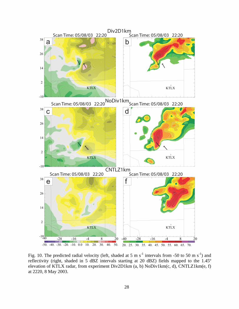
28

Fig. 10. The predicted radial velocity (left, shaded at 5 m s-1 intervals from -50 to 50 m s-1) and reflectivity (right, shaded in 5 dBZ intervals starting at 20 dBZ) fields mapped to the 1.45º elevation of KTLX radar, from experiment Div2D1km (a, b) NoDiv1km(c, d), CNTLZ1km(e, f) at 2220, 8 May 2003.

-10

2

14

26

38

KTLX

-10

2

14

26

38

KTLX

-40 -28 -16 -4 8 20-10

2

14

26

38

-50. -40. -30. -20. -10. 0.0 10. 20. 30. 40. 50.

KTLX

KTLX

KTLX

-40 -28 -16 -4 8 20

20. 25. 30. 35. 40. 45. 50. 55. 60. 65. 70.

KTLX

Div2D1km

NoDiv1km

CNTLZ1km

Scan Time: 05/08/03 22:20 Scan Time: 05/08/03 22:20

Scan Time: 05/08/03 22:20 Scan Time: 05/08/03 22:20

Scan Time: 05/08/03 22:20 Scan Time: 05/08/03 22:20

a b

c d

e f

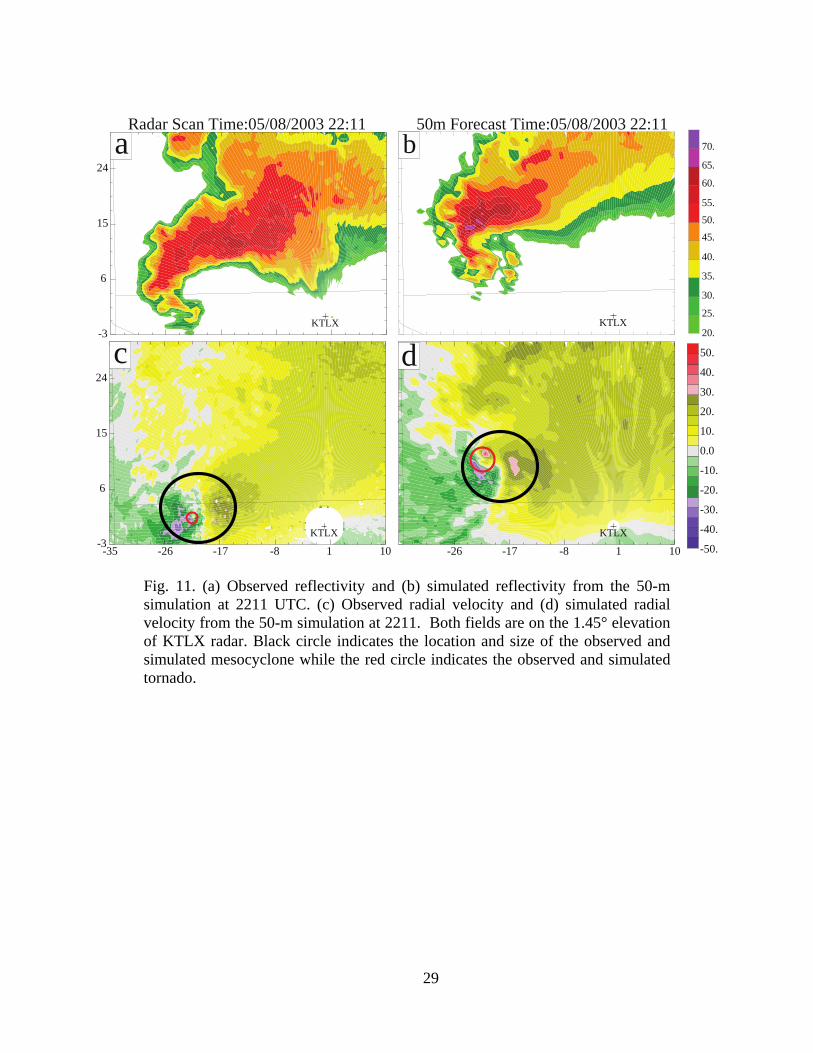
29

Fig. 11. (a) Observed reflectivity and (b) simulated reflectivity from the 50-m simulation at 2211 UTC. (c) Observed radial velocity and (d) simulated radial velocity from the 50-m simulation at 2211. Both fields are on the 1.45° elevation of KTLX radar. Black circle indicates the location and size of the observed and simulated mesocyclone while the red circle indicates the observed and simulated tornado.

-26 -17 -8 1 10 -50.

-40.

-30.

-20.

-10.

0.0

10.

20.

30.

40.

50.

KTLX

-35 -26 -17 -8 1 10-3

6

15

24

KTLX

20.

25.

30.

35.

40.

45.

50.

55.

60.

65.

70.

KTLX-3

6

15

24

Radar Scan Time:05/08/2003 22:11 50m Forecast Time:05/08/2003 22:11

KTLX

a b

dc

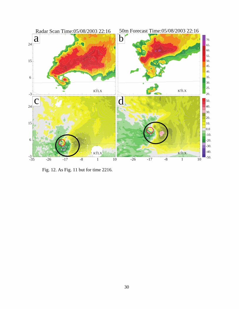
30

Fig. 12. As Fig. 11 but for time 2216.

KTLX-3

6

15

24

KTLX

-26 -17 -8 1 10

KTLX

-35 -26 -17 -8 1 10-3

6

15

24

KTLX

Radar Scan Time:05/08/2003 22:16 50m Forecast Time:05/08/2003 22:16

a b

dc

-50.

-40.

-30.

-20.

-10.

0.0

10.

20.

30.

40.

50.

20.

25.

30.

35.

40.

45.

50.

55.

60.

65.

70.

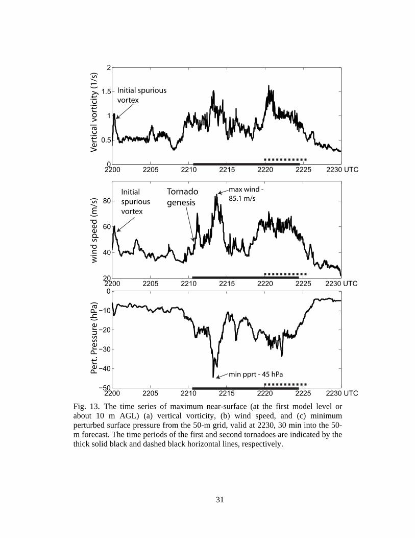
31

Fig. 13. The time series of maximum near-surface (at the first model level or about 10 m AGL) (a) vertical vorticity, (b) wind speed, and (c) minimum perturbed surface pressure from the 50-m grid, valid at 2230, 30 min into the 50-m forecast. The time periods of the first and second tornadoes are indicated by the thick solid black and dashed black horizontal lines, respectively.

2200 2205 2210 2215 2220 2225 2230 UTC0

0.5

1

1.5

2

2200 2205 2210 2215 2220 2225 2230 UTC20

40

60

80

2200 2205 2210 2215 2220 2225 2230 UTC−50

−40

−30

−20

−10

0

Vert

ical

vor

ticity

(1/s

)w

ind

spee

d (m

/s)

Pert

. Pre

ssur

e (h

Pa)

Initial spuriousvortex

Initial spuriousvortex

Tornadogenesis

max wind -85.1 m/s

min pprt - 45 hPa

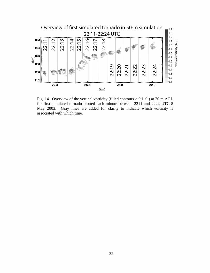
32

Fig. 14. Overview of the vertical vorticity (filled contours > 0.1 s-1) at 20 m AGL for first simulated tornado plotted each minute between 2211 and 2224 UTC 8 May 2003. Gray lines are added for clarity to indicate which vorticity is associated with which time.

22.4 25.6 28.8 32.011.2

12.0

12.8

13.6

14.4

15.2

(km)

(km

)

22.4 25.6 28.8 32.011.2

12.0

12.8

13.6

14.4

15.2

22.4 25.6 28.8 32.011.2

12.0

12.8

13.6

14.4

15.2

22.4 25.6 28.8 32.011.2

12.0

12.8

13.6

14.4

15.2

22.4 25.6 28.8 32.011.2

12.0

12.8

13.6

14.4

15.2

22.4 25.6 28.8 32.011.2

12.0

12.8

13.6

14.4

15.2

22.4 25.6 28.8 32.011.2

12.0

12.8

13.6

14.4

15.2

22.4 25.6 28.8 32.011.2

12.0

12.8

13.6

14.4

15.2

22.4 25.6 28.811.2

12.0

12.8

13.6

14.4

15.2

22.4 25.611.2

12.0

12.8

13.6

14.4

15.2

22.4 25.611.2

12.0

12.8

13.6

14.4

15.2

22.4 25.611.2

12.0

12.8

13.6

14.4

15.2

11.2

12.0

12.8

13.6

14.4

15.2

12.8

14.4

15.2

22:1

1

22:1

2

22:1

3

22:1

422

:15

22:1

622

:17

22:1

8

22:1

922

:20

22:2

1

22:2

2

22:2

3

22:2

4

Overview of first simulated tornado in 50-m simulation22:11-22:24 UTC

0.10.20.30.40.50.60.70.80.91.01.11.21.31.4

Vert

ical

vor

ticity

(1/s

)

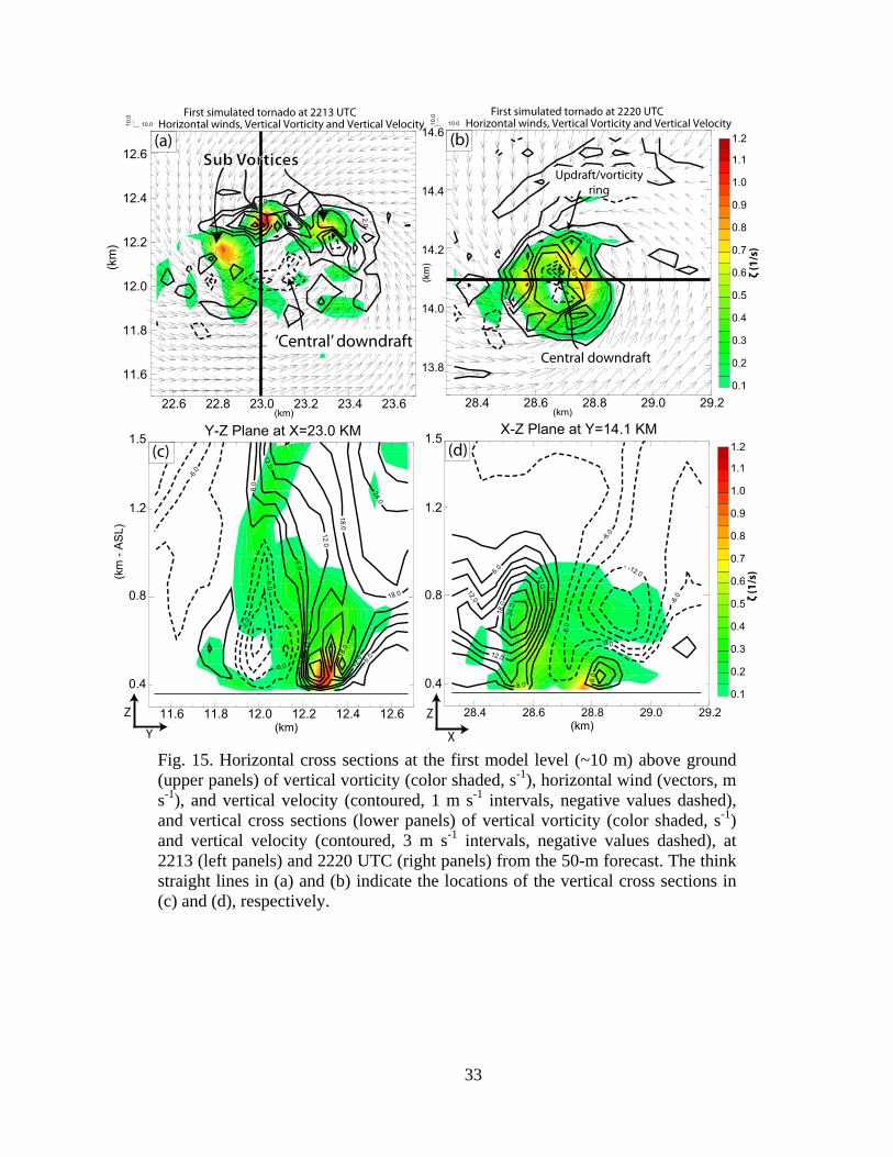
33

Fig. 15. Horizontal cross sections at the first model level (~10 m) above ground (upper panels) of vertical vorticity (color shaded, s-1), horizontal wind (vectors, m s-1), and vertical velocity (contoured, 1 m s-1 intervals, negative values dashed), and vertical cross sections (lower panels) of vertical vorticity (color shaded, s-1) and vertical velocity (contoured, 3 m s-1 intervals, negative values dashed), at 2213 (left panels) and 2220 UTC (right panels) from the 50-m forecast. The think straight lines in (a) and (b) indicate the locations of the vertical cross sections in (c) and (d), respectively.

22.6 22.8 23.0 23.2 23.4 23.6

11.6

11.8

12.0

12.2

12.4

12.6

(km)

(km

)

2.0

2.0

2.0

10.010.0

0.1

0.2

0.3

0.4

0.5

0.6

0.7

0.8

0.9

1.0

1.1

1.2

0.1

0.2

0.3

0.4

0.5

0.6

0.7

0.8

0.9

1.0

1.1

1.2

28.4 28.6 28.8 29.0 29.2

13.8

14.0

14.2

14.4

14.6

(km) (k

m)

2.0

2.0

2.0

2.0

10.010.0

28.4 28.6 28.8 29.0 29.2 (km)

X-Z Plane at Y=14.1 KM

-12.0

-6.0

-6.0

-6.0

-6.0

6.0

6.0

6.0

6.0

12.0

12.0

12.0

18.0

24.0

11.6 11.8 12.0 12.2 12.4 12.6

0.8

0.4

1.2

1.5

(km)

(km

- A

SL)

0.8

0.4

1.2

1.5Y-Z Plane at X=23.0 KM

-6.0

-6.0

-6.0

-6.0

6.0

6.0

6.0 6.0

12.0

12.0

12.0

12.0

18.0

18.0

18.0

24.0

Z

Y

Z

X

First simulated tornado at 2220 UTCHorizontal winds, Vertical Vorticity and Vertical Velocity

First simulated tornado at 2213 UTCHorizontal winds, Vertical Vorticity and Vertical Velocity

Sub VorticesSub Vortices

‘Central’ downdraftCentral downdraft

Updraft/vorticity ring

ζ (1

/s)

ζ (1

/s)

(a) (b)

(c) (d)

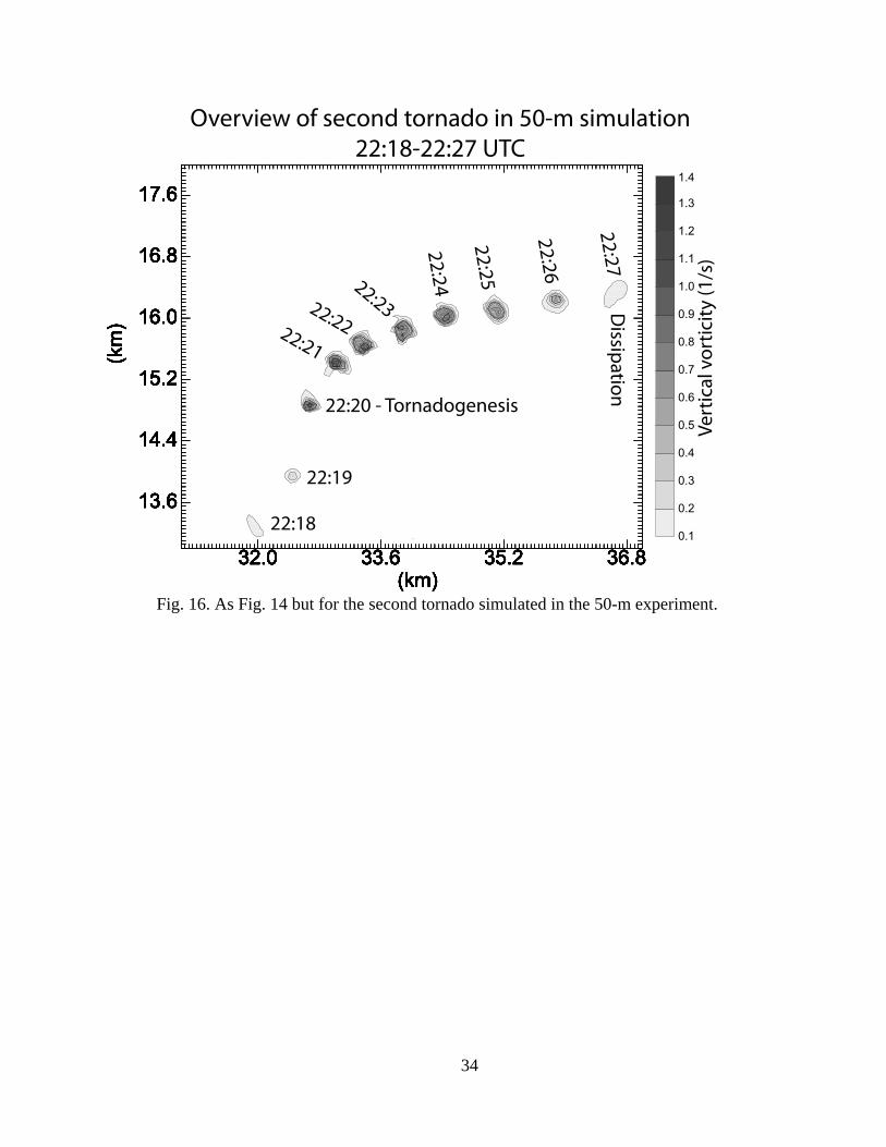
34

Fig. 16. As Fig. 14 but for the second tornado simulated in the 50-m experiment.

0.1

0.2

0.3

0.4

0.5

0.6

0.7

0.8

0.9

1.0

1.1

1.2

1.3

1.4

32.0 33.6 35.2 36.8

13.6

14.4

15.2

16.0

16.8

17.6

(km)

(km

)

32.0 33.6 35.2 36.8

13.6

14.4

15.2

16.0

16.8

17.6

(km)

(km

)

32.0 33.6 35.2 36.8

13.6

14.4

15.2

16.0

16.8

17.6

(km)

(km

)

32.0 33.6 35.2 36.8

13.6

14.4

15.2

16.0

16.8

17.6

(km)

(km

)

32.0 33.6 35.2 36.8

13.6

14.4

15.2

16.0

16.8

17.6

(km)

(km

)

32.0 33.6 35.2 36.8

13.6

14.4

15.2

16.0

16.8

17.6

(km)

(km

)

32.0 33.6 35.2 36.8

13.6

14.4

15.2

16.0

16.8

17.6

(km)

(km

)

32.0 33.6 35.2 36.8

13.6

14.4

15.2

16.0

16.8

17.6

(km)

(km

)

32.0 33.6 35.2 36.8

13.6

14.4

15.2

16.0

16.8

17.6

(km)

(km

)

32.0 33.6 35.2 36.8

13.6

14.4

15.2

16.0

16.8

17.6

(km)

(km

)

22:18

22:19

22:21

22:22

22:23

22:24

22:25

22:26

22:27

22:20 - Tornadogenesis

Dissipation

Overview of second tornado in 50-m simulation22:18-22:27 UTC

Vert

ical

vor

ticity

(1/s

)

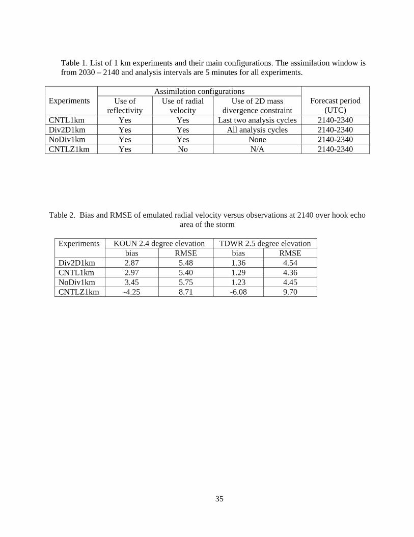
35

Table 1. List of 1 km experiments and their main configurations. The assimilation window is from 2030 – 2140 and analysis intervals are 5 minutes for all experiments.

Experiments

Assimilation configurations Forecast period

(UTC) Use of

reflectivity Use of radial

velocity Use of 2D mass

divergence constraint CNTL1km Yes Yes Last two analysis cycles 2140-2340 Div2D1km Yes Yes All analysis cycles 2140-2340 NoDiv1km Yes Yes None 2140-2340 CNTLZ1km Yes No N/A 2140-2340

Table 2. Bias and RMSE of emulated radial velocity versus observations at 2140 over hook echo area of the storm

Experiments KOUN 2.4 degree elevation TDWR 2.5 degree elevation

bias RMSE bias RMSE Div2D1km 2.87 5.48 1.36 4.54 CNTL1km 2.97 5.40 1.29 4.36 NoDiv1km 3.45 5.75 1.23 4.45 CNTLZ1km -4.25 8.71 -6.08 9.70