Embed Size (px)
Citation preview
International Journal of Mathematics Trends and Technology (IJMTT) – Volume 66 Issue 3- March 2020
ISSN: 2231-5373 http://www.ijmttjournal.org Page 53
Numerical Simulation of Biodiversity Loss:
Comparison of Numerical Methods Godspower C. Abanum
1, Charles O. Omoregbe
2 and Enu-Obari. N. Ekakaa
3
1Department of Mathematics/Statistics, Ignatius Ajuru University of Education, Port Harcourt, Nigeria 2Department of Mathematics/Statistics, University of Port Harcourt, Port Harcourt, Nigeria
3Department of Mathematics/Statistics, Rivers State University, Port Harcourt, Nigeria
ABSTRACT
The dependent variable called Normal Agriculture changes as the independent variable time changes that
is the yields of a normal agriculture variable changes deterministically as the length of the growing season
changes when all the model parameter values are fixed. However, when the model parameter values
𝛼1 𝑎𝑛𝑑 𝛼2are decrease, the normal agricultural variable also changes. By comparing the patterns of
growth in these two interacting normal agricultural data, we have finite instance of biodiversity due to the
application of four numerical methods such as ODE45, ODE23, ODE23tb and ODE15s. We have found
the numerical prediction upon using these four numerical methods which are similar and robust, hence we
have considered ODE45 numerical simulation to be computationally more efficient than the other three
methods. The novel result we have obtained in this study have not been seen elsewhere. These are
presented and discussed quantitatively.
KEYWORD: ODE45,ODE23, ODE23tb, ODE15s, Normal Agriculture
I. INTRODUCTION
Modeling and simulation of dynamical systems has always been an important issue in both science and
engineering. In modern mathematics, the subject of ordinary differential equation has become an effective
tool in the world of mathematical modelling. Most physical phenomena such as biological model, fluid
dynamics, control theory etc are often transform into ordinary differential equations to give explicit
interpretation of the physical attributes of the model in equation.
The effectiveness of these equation in the business of modelling has prompted researchers in developing
methods for seeking solution to these equations. Differential equations model real life situation and provide
real life answers with the help of computer calculations and simulations [7]
The notion to apply ordinary differential system or equation base on system dynamics to investigate the
interaction between ecospheric asset, industrial asset and agricultural wealth or asset begins in 1994 with
the pioneering work of Apedaile et al, it was then followed by the work of Solomonovich et al [17],
Freedom et al [1] and Agyeman et al [2]. Agyeman and Feedom [4] model the interaction between normal
agricultural asset, auxiliary agricultural asset, industrial asset and ecospheric asset using a system of
ordinary differential equation for nonlinear case. They studied the long term effect of each of the assets on
each other, local, global analysis of equilibra of systems and dissipativity solutions are checked and the
conditions for existence of positive interior equilibrium using the theory of uniform persistence were
established. The condition for existence and persistence to occur were proved. [18]Modeled the impacts of
disease and pest on agricultural systems. They provide a brief overview of the recent state of development
in coupling disease and pest models to crops models and explained the scientific and the technical
challenges. They proposed a five-stage road map to improve the simulation of the impacts caused by plant
International Journal of Mathematics Trends and Technology (IJMTT) – Volume 66 Issue 3- March 2020
ISSN: 2231-5373 http://www.ijmttjournal.org Page 54
pests and diseases. Other related contributions to knowledge in the context of environmental modelling of
the interaction of ecosphere, industry and agriculture can be seen in the work of [1-20]
II. MATHEMATICAL FORMULATION
Following Ibrahim A and Freedom H.I (2009), we have consider the four system of nonlinear ordinary
differential equation.
𝑑𝑥1(𝑡)
𝑑𝑡= 𝛼1𝑥1𝑧 − 𝛽1𝑥1
2 + 𝛾1𝑥1𝑦 − 𝜌1𝑥1𝑥2 − 𝜃𝑥1 + 𝜃𝑥1𝑧
𝑑𝑥2(𝑡)
𝑑𝑡= 𝛼2𝑥2𝑧 − 𝛽2𝑥2
2 − 𝛾2𝑥2𝑦 − 𝜌2𝑥1𝑥2
𝑑𝑦(𝑡)
𝑑𝑡= −𝜉𝑦 − 𝜂𝑦2 + 𝛿𝑥1𝑦
𝑑𝑧(𝑡)
𝑑𝑡= −𝜅𝑥1𝑧 + 𝜅1𝑧 − 𝜅1𝑧
2 + 𝜅2𝑥1 − 𝜅2𝑥1𝑧
where all parameters are assumed to be positive constants except 𝛾1 which can be any real constant. 𝛼1(𝛼2)
is inter competitive growth rate coefficient of normal (auxiliary) agriculture due to normal (auxiliary)
agricultural activity for fixed z; 𝛽1(𝛽2) is the per asset diminishing returns rate coefficient for normal
(auxiliary) agriculture in the absence of industry and auxiliary (normal) agriculture, 𝛾1(𝛾2 ) is the per asset
terms of trade coefficient between normal (auxiliary) agriculture and industry, 𝜉 is the constant
depreciation rate coefficient of industry, 𝜂 is the per asset (linear) depreciation rate coefficient of industry,
𝛿 is the per asset growth rate for industry in dealing with normal agriculture, 𝜌1(𝜌2) is the per asset
competitive rate coefficient of auxiliary (normal) agriculture acting on normal (auxiliary) agriculture, 𝜅 is
the per asset degradation rate coefficient of the ecosphere due to normal agricultural activities, 𝜅1 is the
natural restoration rate coefficient for the ecosphere, 𝜅2 is the rate of effort input to restore the ecosphere
by normal agriculture and 𝜃 is the net cost rate to normal agriculture to restore the ecosphere.
With the following precise model parameter values from Agyemang and Freedman (2009)
𝛼1 = 3,𝛼2 = 1 ,𝛽1 =1
10,𝛽2 =
1
10, 𝛾1 = −
1
49,𝛾2 =
1
10,𝜌1 =
1
10, 𝜌2 =
1
5,𝛿 =
1
4,
𝜃 =6
5,𝜂 =
1
20, 𝜉 = 1, 𝜅 = 2,𝜅1 = 2,𝜅2 = 1
III. METHOD OF ANALYSIS
To tackle this environmental problem, we have fully explore the application of four numerical methods,
namely ODE45, ODE23, ODE23tb, ODE15s to model and predict the effect of decreasing 𝛼1 𝑎𝑛𝑑 𝛼2 by
5%, 10% and 15% on a biodiversity loss scenario for a fixed initial condition consisting of a point of
values.
International Journal of Mathematics Trends and Technology (IJMTT) – Volume 66 Issue 3- March 2020
ISSN: 2231-5373 http://www.ijmttjournal.org Page 55
IV. RESULTS
On the application of the above mention four numerical methods, we have obtain the following novel
empirical results which are presented as displayed as shown in table 1- table 12
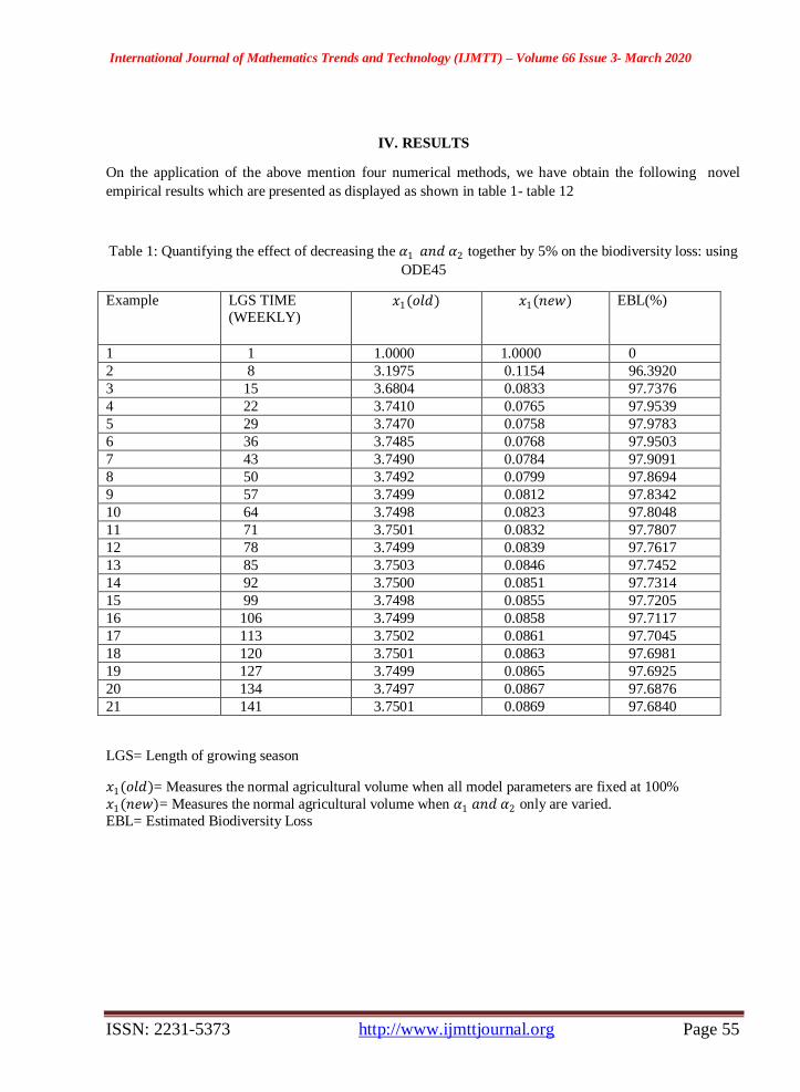
Table 1: Quantifying the effect of decreasing the 𝛼1 𝑎𝑛𝑑 𝛼2 together by 5% on the biodiversity loss: using
ODE45
Example LGS TIME
(WEEKLY) 𝑥1(𝑜𝑙𝑑) 𝑥1(𝑛𝑒𝑤) EBL(%)
1 1 1.0000 1.0000 0
2 8 3.1975 0.1154 96.3920
3 15 3.6804 0.0833 97.7376
4 22 3.7410 0.0765 97.9539
5 29 3.7470 0.0758 97.9783
6 36 3.7485 0.0768 97.9503
7 43 3.7490 0.0784 97.9091
8 50 3.7492 0.0799 97.8694
9 57 3.7499 0.0812 97.8342
10 64 3.7498 0.0823 97.8048
11 71 3.7501 0.0832 97.7807
12 78 3.7499 0.0839 97.7617
13 85 3.7503 0.0846 97.7452
14 92 3.7500 0.0851 97.7314
15 99 3.7498 0.0855 97.7205
16 106 3.7499 0.0858 97.7117
17 113 3.7502 0.0861 97.7045
18 120 3.7501 0.0863 97.6981
19 127 3.7499 0.0865 97.6925
20 134 3.7497 0.0867 97.6876
21 141 3.7501 0.0869 97.6840
LGS= Length of growing season
𝑥1(𝑜𝑙𝑑)= Measures the normal agricultural volume when all model parameters are fixed at 100%
𝑥1(𝑛𝑒𝑤)= Measures the normal agricultural volume when 𝛼1 𝑎𝑛𝑑 𝛼2 only are varied.
EBL= Estimated Biodiversity Loss
International Journal of Mathematics Trends and Technology (IJMTT) – Volume 66 Issue 3- March 2020
ISSN: 2231-5373 http://www.ijmttjournal.org Page 56
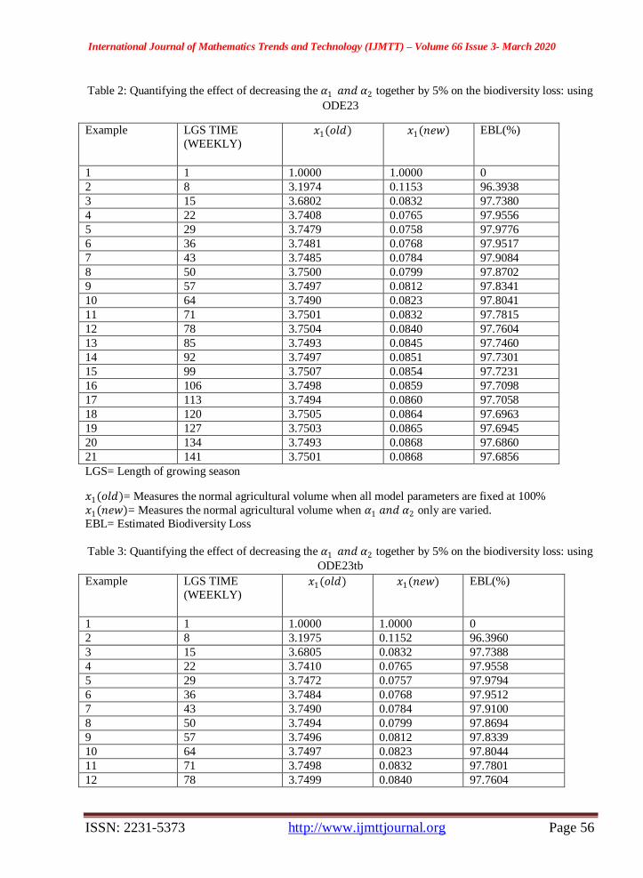
Table 2: Quantifying the effect of decreasing the 𝛼1 𝑎𝑛𝑑 𝛼2 together by 5% on the biodiversity loss: using
ODE23
Example LGS TIME
(WEEKLY) 𝑥1(𝑜𝑙𝑑) 𝑥1(𝑛𝑒𝑤) EBL(%)
1 1 1.0000 1.0000 0
2 8 3.1974 0.1153 96.3938
3 15 3.6802 0.0832 97.7380
4 22 3.7408 0.0765 97.9556
5 29 3.7479 0.0758 97.9776
6 36 3.7481 0.0768 97.9517
7 43 3.7485 0.0784 97.9084
8 50 3.7500 0.0799 97.8702
9 57 3.7497 0.0812 97.8341
10 64 3.7490 0.0823 97.8041
11 71 3.7501 0.0832 97.7815
12 78 3.7504 0.0840 97.7604
13 85 3.7493 0.0845 97.7460
14 92 3.7497 0.0851 97.7301
15 99 3.7507 0.0854 97.7231
16 106 3.7498 0.0859 97.7098
17 113 3.7494 0.0860 97.7058
18 120 3.7505 0.0864 97.6963
19 127 3.7503 0.0865 97.6945
20 134 3.7493 0.0868 97.6860
21 141 3.7501 0.0868 97.6856
LGS= Length of growing season
𝑥1(𝑜𝑙𝑑)= Measures the normal agricultural volume when all model parameters are fixed at 100%
𝑥1(𝑛𝑒𝑤)= Measures the normal agricultural volume when 𝛼1 𝑎𝑛𝑑 𝛼2 only are varied.
EBL= Estimated Biodiversity Loss
Table 3: Quantifying the effect of decreasing the 𝛼1 𝑎𝑛𝑑 𝛼2 together by 5% on the biodiversity loss: using
ODE23tb
Example LGS TIME
(WEEKLY) 𝑥1(𝑜𝑙𝑑) 𝑥1(𝑛𝑒𝑤) EBL(%)
1 1 1.0000 1.0000 0
2 8 3.1975 0.1152 96.3960
3 15 3.6805 0.0832 97.7388
4 22 3.7410 0.0765 97.9558
5 29 3.7472 0.0757 97.9794
6 36 3.7484 0.0768 97.9512
7 43 3.7490 0.0784 97.9100
8 50 3.7494 0.0799 97.8694
9 57 3.7496 0.0812 97.8339
10 64 3.7497 0.0823 97.8044
11 71 3.7498 0.0832 97.7801
12 78 3.7499 0.0840 97.7604
International Journal of Mathematics Trends and Technology (IJMTT) – Volume 66 Issue 3- March 2020
ISSN: 2231-5373 http://www.ijmttjournal.org Page 57
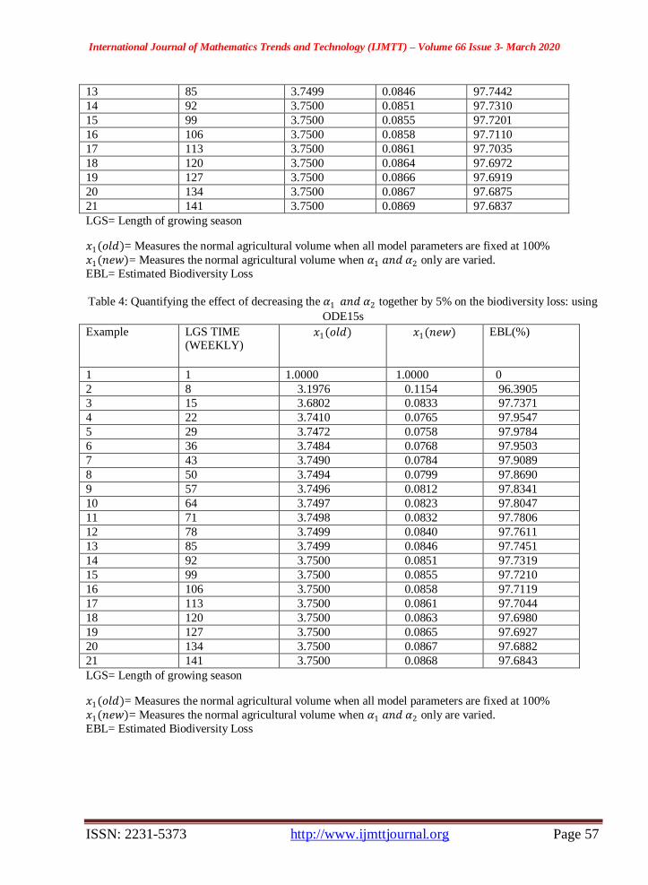
13 85 3.7499 0.0846 97.7442
14 92 3.7500 0.0851 97.7310
15 99 3.7500 0.0855 97.7201
16 106 3.7500 0.0858 97.7110
17 113 3.7500 0.0861 97.7035
18 120 3.7500 0.0864 97.6972
19 127 3.7500 0.0866 97.6919
20 134 3.7500 0.0867 97.6875
21 141 3.7500 0.0869 97.6837
LGS= Length of growing season
𝑥1(𝑜𝑙𝑑)= Measures the normal agricultural volume when all model parameters are fixed at 100%
𝑥1(𝑛𝑒𝑤)= Measures the normal agricultural volume when 𝛼1 𝑎𝑛𝑑 𝛼2 only are varied.
EBL= Estimated Biodiversity Loss
Table 4: Quantifying the effect of decreasing the 𝛼1 𝑎𝑛𝑑 𝛼2 together by 5% on the biodiversity loss: using
ODE15s
Example LGS TIME (WEEKLY)
𝑥1(𝑜𝑙𝑑) 𝑥1(𝑛𝑒𝑤) EBL(%)
1 1 1.0000 1.0000 0
2 8 3.1976 0.1154 96.3905
3 15 3.6802 0.0833 97.7371
4 22 3.7410 0.0765 97.9547
5 29 3.7472 0.0758 97.9784
6 36 3.7484 0.0768 97.9503
7 43 3.7490 0.0784 97.9089
8 50 3.7494 0.0799 97.8690
9 57 3.7496 0.0812 97.8341
10 64 3.7497 0.0823 97.8047
11 71 3.7498 0.0832 97.7806
12 78 3.7499 0.0840 97.7611
13 85 3.7499 0.0846 97.7451
14 92 3.7500 0.0851 97.7319
15 99 3.7500 0.0855 97.7210
16 106 3.7500 0.0858 97.7119
17 113 3.7500 0.0861 97.7044
18 120 3.7500 0.0863 97.6980
19 127 3.7500 0.0865 97.6927
20 134 3.7500 0.0867 97.6882
21 141 3.7500 0.0868 97.6843
LGS= Length of growing season
𝑥1(𝑜𝑙𝑑)= Measures the normal agricultural volume when all model parameters are fixed at 100%
𝑥1(𝑛𝑒𝑤)= Measures the normal agricultural volume when 𝛼1 𝑎𝑛𝑑 𝛼2 only are varied.
EBL= Estimated Biodiversity Loss
International Journal of Mathematics Trends and Technology (IJMTT) – Volume 66 Issue 3- March 2020
ISSN: 2231-5373 http://www.ijmttjournal.org Page 58
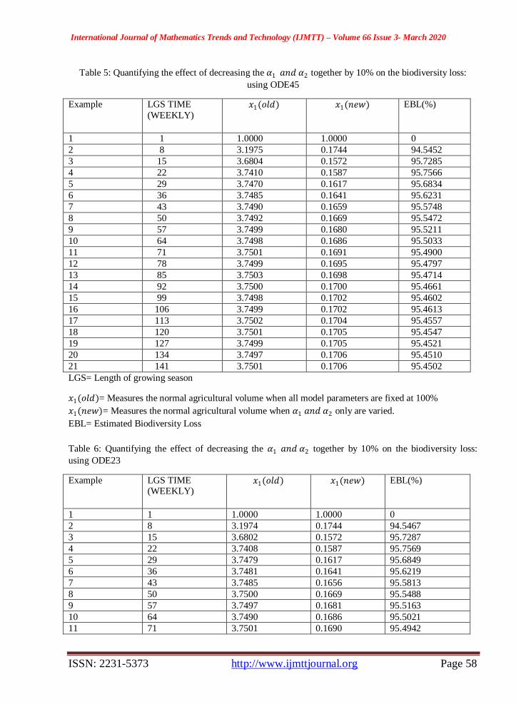
Table 5: Quantifying the effect of decreasing the 𝛼1 𝑎𝑛𝑑 𝛼2 together by 10% on the biodiversity loss:
using ODE45
Example LGS TIME
(WEEKLY) 𝑥1(𝑜𝑙𝑑) 𝑥1(𝑛𝑒𝑤) EBL(%)
1 1 1.0000 1.0000 0
2 8 3.1975 0.1744 94.5452
3 15 3.6804 0.1572 95.7285
4 22 3.7410 0.1587 95.7566
5 29 3.7470 0.1617 95.6834
6 36 3.7485 0.1641 95.6231
7 43 3.7490 0.1659 95.5748
8 50 3.7492 0.1669 95.5472
9 57 3.7499 0.1680 95.5211
10 64 3.7498 0.1686 95.5033
11 71 3.7501 0.1691 95.4900
12 78 3.7499 0.1695 95.4797
13 85 3.7503 0.1698 95.4714
14 92 3.7500 0.1700 95.4661
15 99 3.7498 0.1702 95.4602
16 106 3.7499 0.1702 95.4613
17 113 3.7502 0.1704 95.4557
18 120 3.7501 0.1705 95.4547
19 127 3.7499 0.1705 95.4521
20 134 3.7497 0.1706 95.4510
21 141 3.7501 0.1706 95.4502
LGS= Length of growing season
𝑥1(𝑜𝑙𝑑)= Measures the normal agricultural volume when all model parameters are fixed at 100%
𝑥1(𝑛𝑒𝑤)= Measures the normal agricultural volume when 𝛼1 𝑎𝑛𝑑 𝛼2 only are varied.
EBL= Estimated Biodiversity Loss
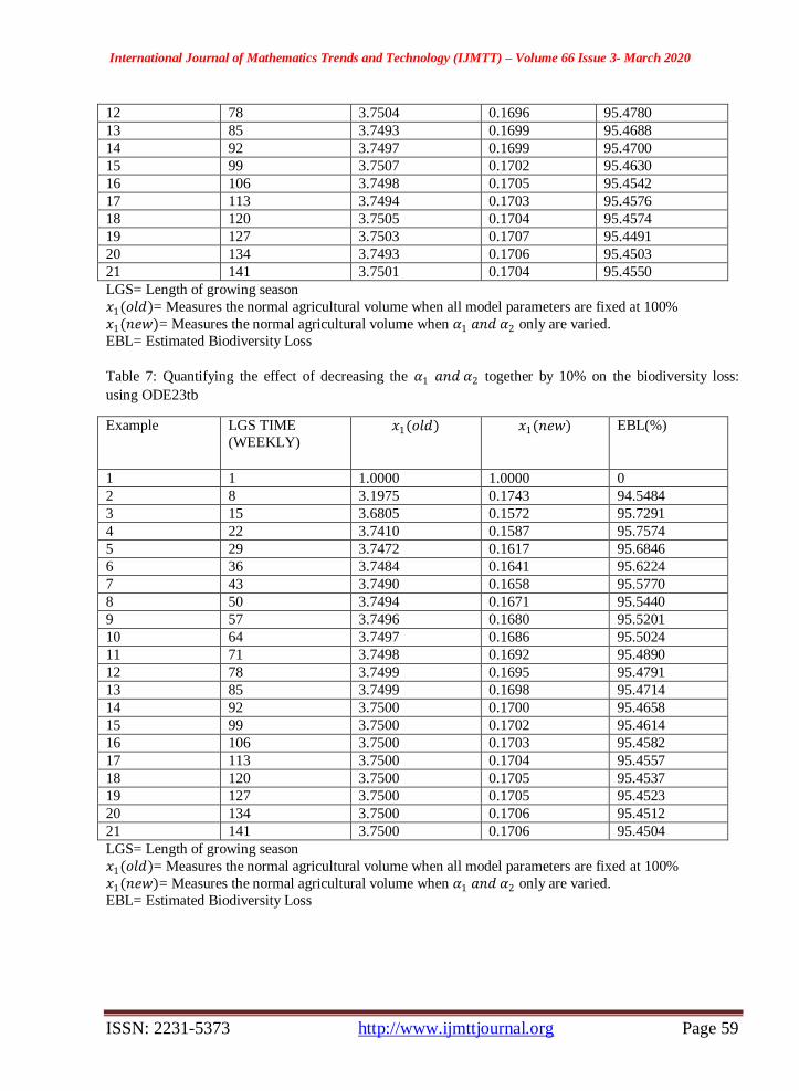
Table 6: Quantifying the effect of decreasing the 𝛼1 𝑎𝑛𝑑 𝛼2 together by 10% on the biodiversity loss:
using ODE23
Example LGS TIME (WEEKLY)
𝑥1(𝑜𝑙𝑑) 𝑥1(𝑛𝑒𝑤) EBL(%)
1 1 1.0000 1.0000 0
2 8 3.1974 0.1744 94.5467
3 15 3.6802 0.1572 95.7287
4 22 3.7408 0.1587 95.7569
5 29 3.7479 0.1617 95.6849
6 36 3.7481 0.1641 95.6219
7 43 3.7485 0.1656 95.5813
8 50 3.7500 0.1669 95.5488
9 57 3.7497 0.1681 95.5163
10 64 3.7490 0.1686 95.5021
11 71 3.7501 0.1690 95.4942
International Journal of Mathematics Trends and Technology (IJMTT) – Volume 66 Issue 3- March 2020
ISSN: 2231-5373 http://www.ijmttjournal.org Page 59
12 78 3.7504 0.1696 95.4780
13 85 3.7493 0.1699 95.4688
14 92 3.7497 0.1699 95.4700
15 99 3.7507 0.1702 95.4630
16 106 3.7498 0.1705 95.4542
17 113 3.7494 0.1703 95.4576
18 120 3.7505 0.1704 95.4574
19 127 3.7503 0.1707 95.4491
20 134 3.7493 0.1706 95.4503
21 141 3.7501 0.1704 95.4550
LGS= Length of growing season
𝑥1(𝑜𝑙𝑑)= Measures the normal agricultural volume when all model parameters are fixed at 100%
𝑥1(𝑛𝑒𝑤)= Measures the normal agricultural volume when 𝛼1 𝑎𝑛𝑑 𝛼2 only are varied.
EBL= Estimated Biodiversity Loss
Table 7: Quantifying the effect of decreasing the 𝛼1 𝑎𝑛𝑑 𝛼2 together by 10% on the biodiversity loss:
using ODE23tb
Example LGS TIME
(WEEKLY) 𝑥1(𝑜𝑙𝑑) 𝑥1(𝑛𝑒𝑤) EBL(%)
1 1 1.0000 1.0000 0
2 8 3.1975 0.1743 94.5484
3 15 3.6805 0.1572 95.7291
4 22 3.7410 0.1587 95.7574
5 29 3.7472 0.1617 95.6846
6 36 3.7484 0.1641 95.6224
7 43 3.7490 0.1658 95.5770
8 50 3.7494 0.1671 95.5440
9 57 3.7496 0.1680 95.5201
10 64 3.7497 0.1686 95.5024
11 71 3.7498 0.1692 95.4890
12 78 3.7499 0.1695 95.4791
13 85 3.7499 0.1698 95.4714
14 92 3.7500 0.1700 95.4658
15 99 3.7500 0.1702 95.4614
16 106 3.7500 0.1703 95.4582
17 113 3.7500 0.1704 95.4557
18 120 3.7500 0.1705 95.4537
19 127 3.7500 0.1705 95.4523
20 134 3.7500 0.1706 95.4512
21 141 3.7500 0.1706 95.4504
LGS= Length of growing season
𝑥1(𝑜𝑙𝑑)= Measures the normal agricultural volume when all model parameters are fixed at 100%
𝑥1(𝑛𝑒𝑤)= Measures the normal agricultural volume when 𝛼1 𝑎𝑛𝑑 𝛼2 only are varied.
EBL= Estimated Biodiversity Loss
International Journal of Mathematics Trends and Technology (IJMTT) – Volume 66 Issue 3- March 2020
ISSN: 2231-5373 http://www.ijmttjournal.org Page 60
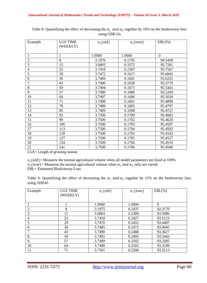
Table 8: Quantifying the effect of decreasing the 𝛼1 𝑎𝑛𝑑 𝛼2 together by 10% on the biodiversity loss:
using ODE15s
Example LGS TIME
(WEEKLY) 𝑥1(𝑜𝑙𝑑) 𝑥1(𝑛𝑒𝑤) EBL(%)
1 1 1.0000 1.0000 0
2 8 3.1976 0.1745 94.5438
3 15 3.6802 0.1572 95.7281
4 22 3.7410 0.1587 95.7567
5 29 3.7472 0.1617 95.6845
6 36 3.7484 0.1641 95.6225
7 43 3.7490 0.1658 95.5770
8 50 3.7494 0.1671 95.5441
9 57 3.7496 0.1680 95.5204
10 64 3.7497 0.1686 95.5030
11 71 3.7498 0.1691 95.4898
12 78 3.7499 0.1695 95.4797
13 85 3.7499 0.1698 95.4721
14 92 3.7500 0.1700 95.4663
15 99 3.7500 0.1702 95.4620
16 106 3.7500 0.1703 95.4587
17 113 3.7500 0.1704 95.4562
18 120 3.7500 0.1705 95.4542
19 127 3.7500 0.1705 95.4527
20 134 3.7500 0.1706 95.4516
21 141 3.7500 0.1706 95.4506
LGS= Length of growing season
𝑥1(𝑜𝑙𝑑)= Measures the normal agricultural volume when all model parameters are fixed at 100%
𝑥1(𝑛𝑒𝑤)= Measures the normal agricultural volume when 𝛼1 𝑎𝑛𝑑 𝛼2 only are varied.
EBL= Estimated Biodiversity Loss
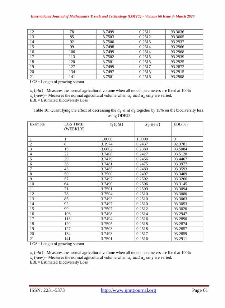
Table 9: Quantifying the effect of decreasing the 𝛼1 𝑎𝑛𝑑 𝛼2 together by 15% on the biodiversity loss:
using ODE45
Example LGS TIME
(WEEKLY) 𝑥1(𝑜𝑙𝑑) 𝑥1(𝑛𝑒𝑤) EBL(%)
1 1 1.0000 1.0000 0
2 8 3.1975 0.2437 92.3770
3 15 3.6804 0.2389 93.5086
4 22 3.7410 0.2427 93.5123
5 29 3.7470 0.2455 93.4487
6 36 3.7485 0.2472 93.4045
7 43 3.7490 0.2488 93.3627
8 50 3.7492 0.2495 93.3442
9 57 3.7499 0.2502 93.3285
10 64 3.7498 0.2505 93.3199
11 71 3.7501 0.2508 93.3113
International Journal of Mathematics Trends and Technology (IJMTT) – Volume 66 Issue 3- March 2020
ISSN: 2231-5373 http://www.ijmttjournal.org Page 61
12 78 3.7499 0.2511 93.3036
13 85 3.7503 0.2512 93.3005
14 92 3.7500 0.2515 93.2937
15 99 3.7498 0.2514 93.2966
16 106 3.7499 0.2514 93.2968
17 113 3.7502 0.2515 93.2939
18 120 3.7501 0.2515 93.2925
19 127 3.7499 0.2517 93.2872
20 134 3.7497 0.2515 93.2915
21 141 3.7501 0.2516 93.2908
LGS= Length of growing season
𝑥1(𝑜𝑙𝑑)= Measures the normal agricultural volume when all model parameters are fixed at 100%
𝑥1(𝑛𝑒𝑤)= Measures the normal agricultural volume when 𝛼1 𝑎𝑛𝑑 𝛼2 only are varied.
EBL= Estimated Biodiversity Loss
Table 10: Quantifying the effect of decreasing the 𝛼1 𝑎𝑛𝑑 𝛼2 together by 15% on the biodiversity loss:
using ODE23
Example LGS TIME
(WEEKLY) 𝑥1(𝑜𝑙𝑑) 𝑥1(𝑛𝑒𝑤) EBL(%)
1 1 1.0000 1.0000 0
2 8 3.1974 0.2437 92.3781
3 15 3.6802 0.2389 93.5084
4 22 3.7408 0.2427 93.5120
5 29 3.7479 0.2456 93.4467
6 36 3.7481 0.2475 93.3977
7 43 3.7485 0.2489 93.3593
8 50 3.7500 0.2497 93.3409
9 57 3.7497 0.2502 93.3266
10 64 3.7490 0.2506 93.3145
11 71 3.7501 0.2509 93.3094
12 78 3.7504 0.2510 93.3080
13 85 3.7493 0.2510 93.3063
14 92 3.7497 0.2510 93.3053
15 99 3.7507 0.2512 93.3020
16 106 3.7498 0.2514 93.2947
17 113 3.7494 0.2516 93.2890
18 120 3.7505 0.2518 93.2874
19 127 3.7503 0.2518 93.2857
20 134 3.7493 0.2517 93.2859
21 141 3.7501 0.2516 93.2911
LGS= Length of growing season
𝑥1(𝑜𝑙𝑑)= Measures the normal agricultural volume when all model parameters are fixed at 100%
𝑥1(𝑛𝑒𝑤)= Measures the normal agricultural volume when 𝛼1 𝑎𝑛𝑑 𝛼2 only are varied.
EBL= Estimated Biodiversity Loss
International Journal of Mathematics Trends and Technology (IJMTT) – Volume 66 Issue 3- March 2020
ISSN: 2231-5373 http://www.ijmttjournal.org Page 62
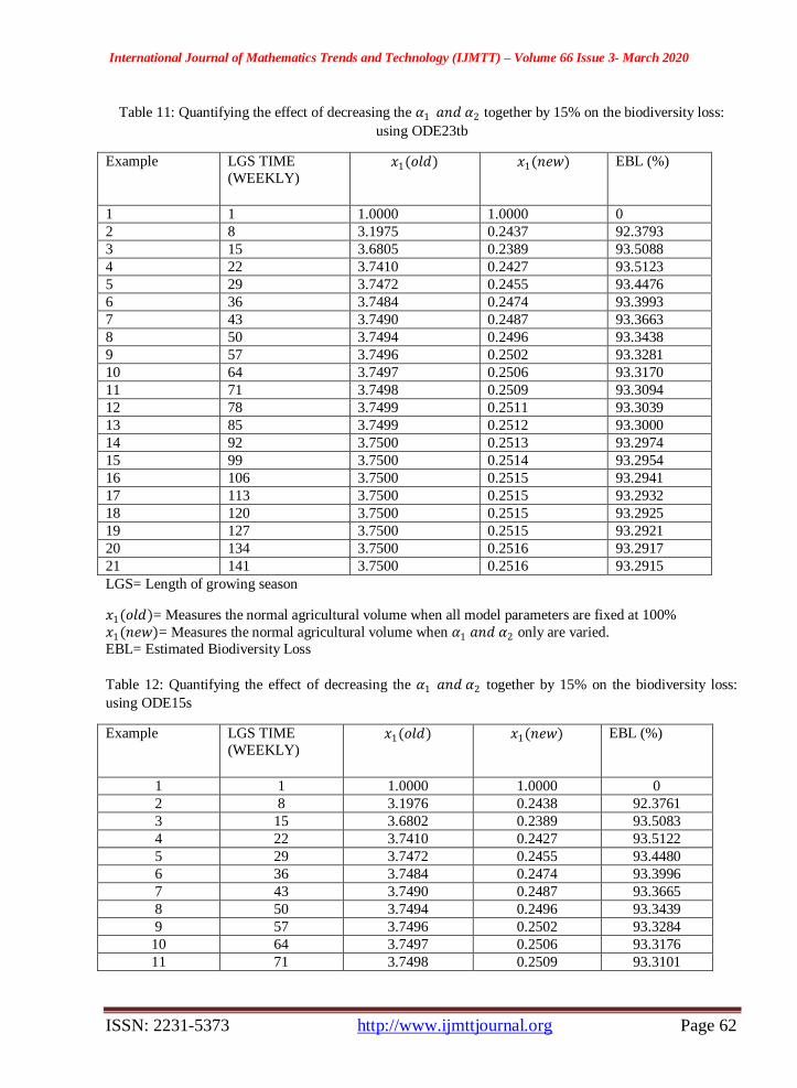
Table 11: Quantifying the effect of decreasing the 𝛼1 𝑎𝑛𝑑 𝛼2 together by 15% on the biodiversity loss:
using ODE23tb
Example LGS TIME
(WEEKLY) 𝑥1(𝑜𝑙𝑑) 𝑥1(𝑛𝑒𝑤) EBL (%)
1 1 1.0000 1.0000 0
2 8 3.1975 0.2437 92.3793
3 15 3.6805 0.2389 93.5088
4 22 3.7410 0.2427 93.5123
5 29 3.7472 0.2455 93.4476
6 36 3.7484 0.2474 93.3993
7 43 3.7490 0.2487 93.3663
8 50 3.7494 0.2496 93.3438
9 57 3.7496 0.2502 93.3281
10 64 3.7497 0.2506 93.3170
11 71 3.7498 0.2509 93.3094
12 78 3.7499 0.2511 93.3039
13 85 3.7499 0.2512 93.3000
14 92 3.7500 0.2513 93.2974
15 99 3.7500 0.2514 93.2954
16 106 3.7500 0.2515 93.2941
17 113 3.7500 0.2515 93.2932
18 120 3.7500 0.2515 93.2925
19 127 3.7500 0.2515 93.2921
20 134 3.7500 0.2516 93.2917
21 141 3.7500 0.2516 93.2915
LGS= Length of growing season
𝑥1(𝑜𝑙𝑑)= Measures the normal agricultural volume when all model parameters are fixed at 100%
𝑥1(𝑛𝑒𝑤)= Measures the normal agricultural volume when 𝛼1 𝑎𝑛𝑑 𝛼2 only are varied.
EBL= Estimated Biodiversity Loss
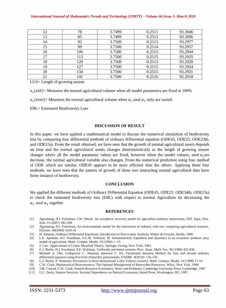
Table 12: Quantifying the effect of decreasing the 𝛼1 𝑎𝑛𝑑 𝛼2 together by 15% on the biodiversity loss:
using ODE15s
Example LGS TIME
(WEEKLY) 𝑥1(𝑜𝑙𝑑) 𝑥1(𝑛𝑒𝑤) EBL (%)
1 1 1.0000 1.0000 0
2 8 3.1976 0.2438 92.3761
3 15 3.6802 0.2389 93.5083
4 22 3.7410 0.2427 93.5122
5 29 3.7472 0.2455 93.4480
6 36 3.7484 0.2474 93.3996
7 43 3.7490 0.2487 93.3665
8 50 3.7494 0.2496 93.3439
9 57 3.7496 0.2502 93.3284
10 64 3.7497 0.2506 93.3176
11 71 3.7498 0.2509 93.3101
International Journal of Mathematics Trends and Technology (IJMTT) – Volume 66 Issue 3- March 2020
ISSN: 2231-5373 http://www.ijmttjournal.org Page 63
12 78 3.7499 0.2511 93.3046
13 85 3.7499 0.2512 93.3006
14 92 3.7500 0.2513 93.2977
15 99 3.7500 0.2514 93.2957
16 106 3.7500 0.2515 93.2944
17 113 3.7500 0.2515 93.2935
18 120 3.7500 0.2515 93.2928
19 127 3.7500 0.2515 93.2924
20 134 3.7500 0.2515 93.2921
21 141 3.7500 0.2516 93.2918
LGS= Length of growing season
𝑥1(𝑜𝑙𝑑)= Measures the normal agricultural volume when all model parameters are fixed at 100%
𝑥1(𝑛𝑒𝑤)= Measures the normal agricultural volume when 𝛼1 𝑎𝑛𝑑 𝛼2 only are varied.
EBL= Estimated Biodiversity Loss
DISCUSSION OF RESULT
In this paper, we have applied a mathematical model to discuss the numerical simulation of biodiversity
loss by comparing four differential methods of ordinary differential equation (ODE45, ODE23, ODE23tb,
and ODE15s). From the result obtained, we have seen that the growth of normal agricultural assets depends
on time and the normal agricultural assets changes deterministically as the length of growing season
changes where all the model parameter values are fixed, however when the model value𝛼1 𝑎𝑛𝑑 𝛼2are
decrease, the normal agricultural variable also changes. From the numerical prediction using four method
of ODE which are similar, ODE45 appears to be more efficient than the others. Applying these four
methods, we have seen that the pattern of growth of these two interacting normal agricultural data have
finite instance of biodiversity.
CONCLUSION
We applied the different methods of Ordinary Differential Equation (ODE45, ODE23. ODE34tb, ODE15s)
to check the estimated biodiversity loss (EBL) with respect to normal Agriculture by decreasing the
𝛼1 𝑎𝑛𝑑 𝛼2 together.
REFERENCES
[1] Agyemang, H.I. Freedman, J.W. Macki, An ecospheric recovery model for agriculture industry interactions, Diff. Eqns. Dyn.
Syst. 15 (2007) 185-208.
[2] Agyemang, H.I. Freedman, An environmental model for the interaction of industry with two competing agricultural resource,
Elsevier. 49(2009) 1618-16
[3] H. Amman, Ordinary Differential Equations: Introduction to Non-Linear Analysis, Walter de Gruyter, Berlin, 1990.
[4] L.P. Apedaile, H.I. Freedman, S.G.M. Schilizzi, M. Solomonovich, Equilibria and dynamics in an economic predator prey
model of agriculture, Math. Comput. Model. 19 (1994) 1 -15.
[5] J. Carr, Applications of Center Manifold Theory, Springer-Verlag, New York, 1981.
[6] G.J. Butler, H.I. Freedman, P.E. Waltman, Uniformly persistent systems, Proc. Amer. Math. Soc. 96 (1986) 425 430.
[7] Michael A. Obe, Godspower C. Abanum, Innocent C. Eli, Variational Iteration Method for first and second ordinary
differential equation using first kind chebychev polynomials, IJASRE. 4(2018) 126-130
[8] G.J. Butler, P. Waltman, Persistence in three-dimensional Lotka Volterra systems, Math. Comput. Model. 10 (1988) 13 16.
[9] C.W. Clark, Mathematical Bioeconomics: The Optimal Management of Renewable Resources, Wiley, New York, 1990.
[10] J.M. Conrad, C.W. Clark, Natural Resource Economics: Notes and Problems, Cambridge University Press, Cambridge, 1987.
[11] G.C. Daily, Natures Services: Societal Dependence on Natural Ecosystem, Island Press, Washington, DC, 1997.
International Journal of Mathematics Trends and Technology (IJMTT) – Volume 66 Issue 3- March 2020
ISSN: 2231-5373 http://www.ijmttjournal.org Page 64
[12] G.C. Daily, K. Ellison, The New Economy of Nature: The Quest to Make Conservation Profitable, Island Press, Washington,
DC, 2002.
[13] G.C. Daily, P.A. Matson, P.M. Vitousek, Ecosystem services supplied by soil, in: Natures Services: Societal Dependence on
Natural Ecosystem, Island Press, Washington, DC, 1997.
[14] L. Edelstein-Keshet, Mathematical Models in Biology, Random House, New York, 1988
[15] H.W. Eves, Foundations and Fundamental Concepts of Mathematics, PWS-Kent, Boston, 1990.
[16] H.I. Freedman, Deterministic Mathematical Models in Population Ecology, Marcel Dekker Inc., New York, 1980.
[17] H.I. Freedman, P. Moson, Persistence definitions and their connections, Proc. Amer. Math. Soc. 109 (1990) 1025 1033.
[18] H.I. Freedman, J.W.-H. So, Global stability and persistence of simple food chains, Math. Biosci. 73 (1985) 89 91.
[19] H.I. Freedman, M. Solomonovich, L.P. Apedaile, A. Hailu, Stability in models of agricultural-industry-environment
interactions, in: Advances in Stability Theory, vol. 13, Taylor and Francis, London, 2003, pp. 255 265.
[20] H.I. Freedman, P. Waltman, Persistence in a model of three competitive populations, Math. Biosci. 73 (1985) 89 91.
[21] H.I. Freedman, P. Waltman, Persistence in a model of three interacting predator-prey populations, Math. Biosci. 68 (1984) 213
231.
[22] G. Heal, Nature and the Marketplace: Capturing the Value of Ecosystem Services, Island Press, Washington, DC, 2000.
[23] L. Horrigan, R.S. Lawrence, P. Walker, How sustainable agriculture can address the environmental and human health harms of
industrial agriculture, Environ. Health Persp. 110: 445 456.
[24] J. Ikerd, The ecology of sustainability, University of Missouri, MO, USA.
[25] J. Ikerd, Sustaining the profitability of agriculture, Paper presented at extension pre-conference, The economists role in the
agricultural sustainability paradigm, San Antonio, TX, 1996.
[26] J.P. LaSalle, The Stability and Control of Discrete Processes, Springer-Verlag, New York, 1986.
[27] N. Myers, The world’s forest and their ecosystem services, in: Natures Services: Societal Dependence on Natural Ecosystem,
Island Press, Washington, DC, 1997.
[28] F. Nani, Mathematical Models of Chemotherapy and Immunotherapy, Ph.D. Thesis, Univ. of Alberta, AB, 1998.
[29] L. Perko, Differential Equations and Dynamical Systems, Springer, New York, 1996.
[30] M. Solomonovich, L.P. Apedaile, H.I. Freedman, A.H. Gebremedihen, S.M.G. Belostotski, Dynamical economic model of
sustainable agriculture and the ecosphere, Appl. Math. Comput. 84 (1997) 221 246.
[31] M. Solomonovich, L.P. Apedaile, H.I. Freedman, Predictability and trapping under conditions of globalization of agricultural
trade: An application of the CGS approach, Math. Comput. Model. 33 (2001) 495 516.
[32] M. Solomonovich, H.I. Freedman, L.P. Apedaile, S.G.M. Schilizzi, L. Belostotski, Stability and bifurcations in an
environmental recovery model of economic agriculture-industry interactions, Natur. Resource Modeling 11 (1998) 35 79.
[33] P.M. Vitousek, H.A. Mooney, J. Lubchenco, J.M. Mellilo, Human domination on earth’s ecosystems, Science 227 (1997)