2009 American WJTA Conference and Expo August 18-20, 2009 • Houston, Texas

Paper

NUMERICAL SIMULATION OF HIGH-SPEED WATER JET FLOW

WITH CAVITATION BY A COMPRESSIBLE MIXTURE FLOW MODEL

G. Peng, S. Shimizu College of Engineering, Nihon University

Koriyama, Fukushima, Japan

S. Fujikawa Graduate School of Engineering, Hokkaido University

Sapporo, Hokkaido, Japan

ABSTRACT A practical mixture flow method is proposed for numerical simulation of high-speed cavitating flow by coupling a bubble cavitation model and a compressible two-phase mixture flow computation. Two-phase fluid media are treated as a mixture composed of a liquid and spherical gas bubbles dispersing in the liquid phase uniformly. Mean flow of the two-phase mixture is calculated by neglecting the slip between bubbles and the liquid phase under the assumption of locally homogeneous medium. Navier-Stokes equations for compressible fluids are used to describe the unsteady flow field of bubble-liquid mixture considering the compressibility of cavitating liquid caused by bubble expansion and contraction, and the RNG k-ε model is adopted for modeling of flow turbulence. The intensity of cavitation in a local field is evaluated by the volume fraction of gas phase varying with the mean flow. Submerged water jet flows in a Venturi nozzle are treated under different cavitation numbers. The result demonstrates that pressure decreases from the inlet to the throat corresponding to the flow convergence and cavitation occurs in the low-pressure region between the wall and the shear layer. Under the influence of cavitation the discharge coefficient decreases to about 60% when σ = 0.1 compared to the case of no-cavitating flow.

Organized and Sponsored by the WaterJet Technology Association

1. INTRODUCTION Cavitation is an important phenomenon often observed in variety of hydraulic systems such as nozzles and hydraulic machineries. Numerical simulation of cavitating flow is of great importance for performance prediction and efficient design of many engineering devices. Modeling of cavitation has been pursued for years and some useful methods have been developed. Egashira et al. (1) proposed a Two-Fluid Three-Pressure Model considering particularities due to the growth and collapse of bubbles, and it demonstrates a possibility to deal with the high-pressure jump caused by cavitation. The two-fluid approach adopted is rational by computing the liquid and gas flows one by one, but the computed flow fields strongly depend upon physical models used for evaluating the interaction between the liquid and bubbles. For the lack of such a general physical model, an extra effort is required for its applications. Cavitation usually takes place in low-pressure regions of relative high velocity and the size of cavitation bubbles is very small compared to its flow field. Bubbles and the working liquid and could be sufficiently well mixed and their relative motion in a small local area is often insignificant. With the aim of flow computation simplification the so-called two-phase flow approach treats the flows of liquid and gas together by assuming that the gas and the liquid phases flow at the same velocity. Owing to its convenience the equal-velocity approach has been widely applied by combined with certain cavitation models. Kubota et al. (2) developed a two-phase bubble cavitation model by coupling a simplified Rayleigh-Plesset equation and an incompressible flow solver, where the bubble expansion is treated attentively but the mixture compressibility is actually neglected although the variation of mixture density is accounted. Iga et al. (3) advanced a compressible homogeneous mixture flow method by adopting a relation of the mixture sonic speed and the gas mass fraction derived under equal pressure assumption, where effects of bubble dynamics are neglected. Considering the difficulty of dealing with both the compressible and incompressible features coexisted in cavitating flows efficiently Peng et al. (4) developed a pressure-based procedure based on CCUP method, and it has been applied to the case of high-speed submerged water jets. Focused on the numerical prediction of cavitatiing flow, this paper presents a simplified compressible mixture flow bubble cavitation model by coupling a bubble cavitation model and a compressible mixture flow computation. Two-phase fluid media of cavitating flow are treated as a mixture of liquid and spherical gas bubbles which are supposed to disperse uniformly in the liquid. Mean flow of the two-phase mixture is treated by Navier-Stokes equations for compressible fluids under the assumption of a locally homogeneous medium and the flow turbulence is modeled by the RNG k-ε model. The intensity of cavitation in a local field is evaluated by the volume fraction of gas phase varying with the mean flow. As an example, submerged water jet flows in a Venturi nozzle are treated under different cavitation numbers, and the reliability of the computation model is confirmed by comparing the results of cavitating and no-cavitating flows.

2. FLOW EQUATIONS AND NUMERICAL APPROACH 2.1 Compressibility of Cavitating Two-phase Fluid Mixture The fluid media of cavitation flow are taken as a two-phase mixture of working liquid and cavitation bubbles. The gas phase is supposed to disperse in the liquid phase and its volume faction is denoted as αG. So, the liquid volume fraction is written to be GL αα −=1 . Then, the density of two-phase mixture can be defined as follows by volume averaging.

GGLLm αραρρ += (1)

where ρ denotes the density and the subscripts L, G and m do the liquid phase, the gas phase and the mixture, respectively. Concerning the compressibility of the two-phase mixture, the variation of mixture density can be derived as follows by taking the differential of above equation.

tdd

tdd

tdd

tdd G

LGL

LG

Gm α

ρρραρ

αρ )( −++= (2)

Considering the continuity of the mixture flow, we arrange it to the following form.

tdd

tdd

tdd L

L

LG

G

Gm

m

ρραρ

ραρ

ρ+=

1 (3)

Concerning the compressibility of the liquid phase the state equation in Tait form is employed.

Ln

L

LL

BpBp

⎟⎟⎠

⎞⎜⎜⎝

⎛=

++

00 ρρ (4)

where the subscript 0 denotes a reference state which is taken to be the atmospheric one. B=3.049×108 Pa, nL =7.15. Then, the compressibility of the liquid phase can be given by the following equation.

( ) tddp

Bpntddp

ctdd L

LL

LL

L

L

+==

ρρ2

1 (5)

where cL denotes the sonic speed in the liquid phase. As for the gas phase it is assumed that gases included in a bubble mainly consist of non-condensation gas, which is taken to be perfect one. Its state equation is given as follows.

Gn

G

G

G

G

pp

⎟⎟⎠

⎞⎜⎜⎝

⎛=

00 ρρ

(6)

where nG is a constant denoting the ratio of specific heat. Then, the compressibility of the gas phase can be given by the following equation.

tddp

pntddp

ctdd G

GG

GG

G

G ρρ== 2

1 (7)

where cG denotes the sonic speed in the gas phase. Taking Eqs (5) and (7) into Eq. (3) we obtain the following equation defining the mean compressibility of the two phase mixture.

tddp

ctddp

ctdd L

LL

LG

GG

Gm

m22

1ρα

ραρ

ρ+= (8)

Here cG denotes the average sonic speed in the two-phase mixture. According to the equation we understand that the compressibility of the two-phase mixture depends upon the volume fraction of gas phase as well as the gas pressure, which is determined by the bubble size. Corresponding to the variation of working pressure bubbles included in a liquid expand a/o contract. The gas pressure at the inside of a bubble is different to the surrounding liquid pressure for the effect of bubble surface acceleration. So, the compressibility of a bubble-liquid mixture should be evaluated based on a careful consideration of bubble dynamics. However, it will take too much time to match the computations of a high frequency bubble surface oscillation and a fluid flow filed. In order to develop a practical method for engineering applications the effect of bubble oscillation is neglected. Then, we know that LGm ppp == , and Eq. (8) is simplified to the following one.

tddp

ctdd L

mm

m

m2

11ρ

ρρ

≅ (9)

where

2221

LL

L

GG

G

mm ccc ρα

ρα

ρ+= (10)

2.2 Turbulent Cavitating Flow Governing Equations As mentioned above fluid media of high-speed cavitating flow are treated as a two-phase mixture consisted of liquid and micro bubbles. Mean flow of the mixture is concerned by neglecting the relative motion of liquid and micro bubbles. For the numerical computation of such a complex flow phenomenon, a reliable viscous flow computation procedure for variable fluid density is required. As main flow governing equations general Reynolds Averaged Navier-Stokes equations for compressible turbulent flow are adopted. Temperature variation caused by growth and collapse of cavitation bubbles is thought to be very small in the whole flow field and thus the conservation equation of energy is omitted. Conservation equations of mass and momentum employed are given in vector form as follows. For convenience the subscript m denoting the mixture is omitted hereafter.

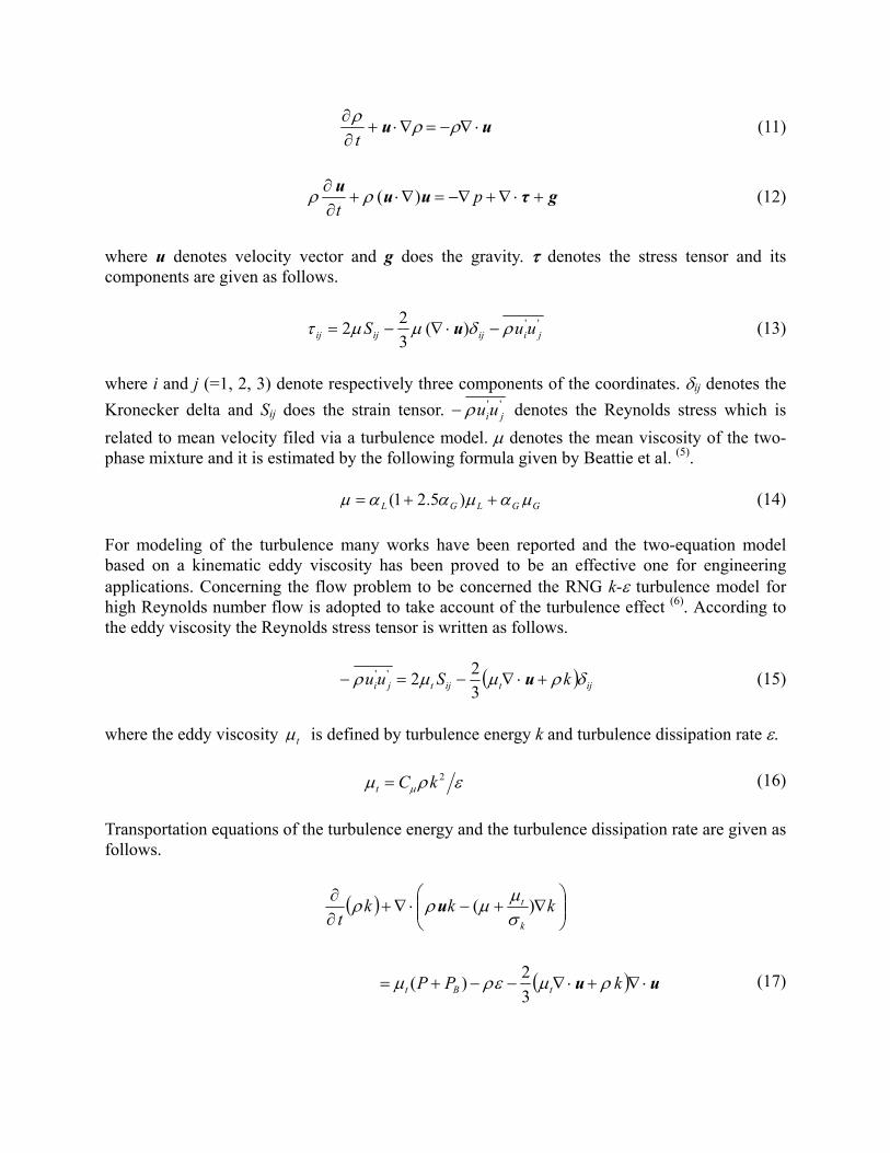
uu ⋅∇−=∇⋅+∂∂ ρρρ

t (11)

gτuuu+⋅∇+−∇=∇⋅+

∂∂ p

t)(ρρ (12)

where u denotes velocity vector and g does the gravity. τ denotes the stress tensor and its components are given as follows.

'')(322 jiijijij uuS ρδμμτ −⋅∇−= u (13)

where i and j (=1, 2, 3) denote respectively three components of the coordinates. δij denotes the Kronecker delta and Sij does the strain tensor. ''

jiuuρ− denotes the Reynolds stress which is related to mean velocity filed via a turbulence model. μ denotes the mean viscosity of the two-phase mixture and it is estimated by the following formula given by Beattie et al. (5).

GGLGL μαμααμ ++= )5.21( (14) For modeling of the turbulence many works have been reported and the two-equation model based on a kinematic eddy viscosity has been proved to be an effective one for engineering applications. Concerning the flow problem to be concerned the RNG k-ε turbulence model for high Reynolds number flow is adopted to take account of the turbulence effect (6). According to the eddy viscosity the Reynolds stress tensor is written as follows.

( ) ijtijtji kSuu δρμμρ +⋅∇−=− u322'' (15)

where the eddy viscosity tμ is defined by turbulence energy k and turbulence dissipation rate ε.

ερμ μ2kCt = (16)

Transportation equations of the turbulence energy and the turbulence dissipation rate are given as follows.

( ) ⎟⎟⎠

⎞⎜⎜⎝

⎛∇+−⋅∇+

∂∂ kkkt k

t )(σμμρρ u

( ) uu ⋅∇+⋅∇−−+= kPP tBt ρμερμ32)( (17)

( )

( ) uuu

u

⋅∇++−⎥⎦⎤

⎢⎣⎡ ⋅∇+⋅∇−=

⎟⎟⎠

⎞⎜⎜⎝

⎛∇+−⋅∇+

∂∂

ερμεερρμμε

εσμμερερ

εεεε

ε

43

2

21 32

)(

CPk

Ck

CkPk

C

t

Bttt

t

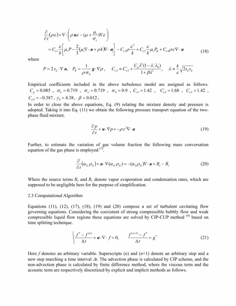
(18)

where

ρσρ

∇⋅=∇⋅= guh

Bij PsP 1,2 , ijij sskCCC 2,

1)1(

30

3~22 ε

λβλ

λλλμεε ≡

+−

+≡

Empirical coefficients included in the above turbulence model are assigned as follows.

085.0=μC , 719.0=kσ , 719.0=εσ , 9.0=hσ , 42.11 =εC , 68.1~2 =εC , 42.13 =εC ,

387.04 −=εC , 38.40 =γ , 012.0=β . In order to close the above equations, Eq. (9) relating the mixture density and pressure is adopted. Taking it into Eq. (11) we obtain the following pressure transport equation of the two-phase fluid mixture.

uu ⋅∇−=∇⋅+∂∂ 2cp

tp ρ (19)

Further, to estimate the variation of gas volume fraction the following mass conversation equation of the gas phase is employed (7).

( ) ceGGGGGG RRt

−+⋅∇−=∇⋅+∂∂ uu )()( ραραρα (20)

Where the source terms Re and Rc denote vapor evaporation and condensation rates, which are supposed to be negligible here for the purpose of simplification. 2.3 Computational Algorithm Equations (11), (12), (17), (18), (19) and (20) compose a set of turbulent cavitating flow governing equations. Considering the coexistent of strong compressible bubbly flow and weak compressible liquid flow regions these equations are solved by CIP-CUP method (4) based on time splitting technique.

⎩⎨⎧

=Δ−

=⋅∇⋅+Δ− +

**)1()(*

,0 gt

ffftff nn

u (21)

Here f denotes an arbitrary variable. Superscripts (n) and (n+1) denote an arbitrary step and a new step marching a time interval Δt. The advection phase is calculated by CIP scheme, and the non-advection phase is calculated by finite difference method, where the viscous term and the acoustic term are respectively discretized by explicit and implicit methods as follows.

⎪⎪⎩

⎪⎪⎨

⎧

⋅∇−=Δ−

+⋅∇+∇−=Δ−

++

+

)1(2**)1(

***

*)1( 1

nn

n

ct

pp

pt

u

gτuu

ρ

ρ (22)

Defining that ( ) tp Δ+⋅∇+∇−+= gτuu ****~ /)( ρ , we derive the following Poisson equation.

ttcpp

Δ⋅∇

=Δ′

−⎟⎟⎠

⎞⎜⎜⎝

⎛ ′∇⋅∇

~

22**u

ρρ (23)

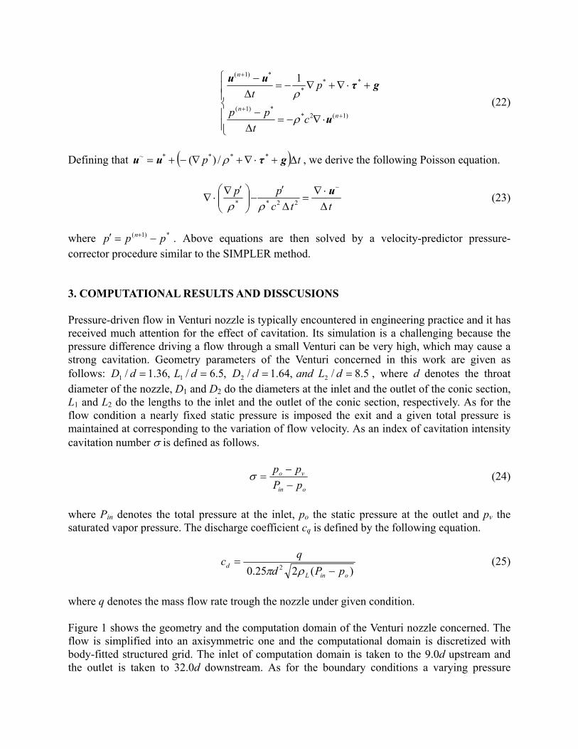
where *)1( ppp n −=′ + . Above equations are then solved by a velocity-predictor pressure-corrector procedure similar to the SIMPLER method. 3. COMPUTATIONAL RESULTS AND DISSCUSIONS

Pressure-driven flow in Venturi nozzle is typically encountered in engineering practice and it has received much attention for the effect of cavitation. Its simulation is a challenging because the pressure difference driving a flow through a small Venturi can be very high, which may cause a strong cavitation. Geometry parameters of the Venturi concerned in this work are given as follows: 5.8/,64.1/,5.6/,36.1/ 2211 ==== dLanddDdLdD , where d denotes the throat diameter of the nozzle, D1 and D2 do the diameters at the inlet and the outlet of the conic section, L1 and L2 do the lengths to the inlet and the outlet of the conic section, respectively. As for the flow condition a nearly fixed static pressure is imposed the exit and a given total pressure is maintained at corresponding to the variation of flow velocity. As an index of cavitation intensity cavitation number σ is defined as follows.

oin

vo

pPpp

−−

=σ (24)

where Pin denotes the total pressure at the inlet, po the static pressure at the outlet and pv the saturated vapor pressure. The discharge coefficient cq is defined by the following equation.

)(225.0 2oinL

d pPdqc

−=

ρπ (25)

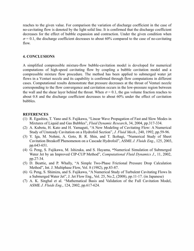
where q denotes the mass flow rate trough the nozzle under given condition. Figure 1 shows the geometry and the computation domain of the Venturi nozzle concerned. The flow is simplified into an axisymmetric one and the computational domain is discretized with body-fitted structured grid. The inlet of computation domain is taken to the 9.0d upstream and the outlet is taken to 32.0d downstream. As for the boundary conditions a varying pressure

condition is imposed at the inlet according to the given total pressure and the actual flow velocity, and a given static pressure is specified at the outlet. All wall boundaries the no-slip condition is applied. At the in-out flow boundary of the cylindrical surface the free flow boundary conditions are imposed.

At first, concerning the structure of no-cavitation flow numerical simulations were performed under a large cavitation number by specifying a discharge pressure high enough for a given driven pressure difference. As an example, Figure 2 shows the distribution of no-cavitaing flow when the driven pressure 010 pp ≅Δ , here p0 denotes the standard atmospheric pressure (σ≥2.5). According to the computation result the mean velocity of well-developed jet flow reaches to 40m/s and the Reynolds number is known to be 5105.4Re ×≅ . Figure 2 (a), (b), (c) and (d) present contour maps of axial velocity u, turbulence kinetic energy k, turbulence dissipation rate ε and pressure p, respectively when the flow is well-developed. As shown in the figures, the flow accelerates in the convergent section and expands in after passing through the throat. In the divergent section a vortex region is formed between the main flow and the solid wall and a small flow separation is demonstrated near the wall just behind the throat. The turbulent kinetic energy is concentrated in the vortex region between the main flow and the solid wall, and the turbulent dissipation takes places in the shear layer as shown in Figure 2 (b) and (c). The mean pressure decreases from the inlet to the throat corresponding to the increase of flow velocity. So, as shown in Figure 2 (d), a low-pressure region is formed near the wall just behind the throat, where cavitation is easy to occur under a small cavitation number.

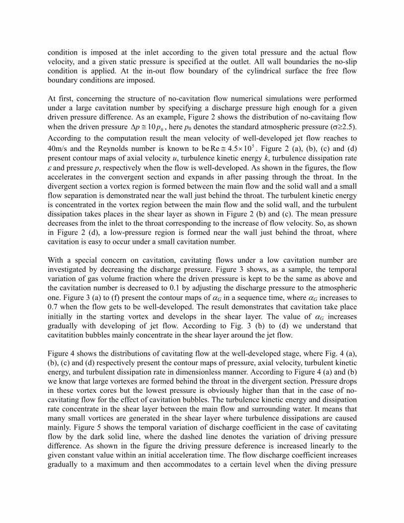
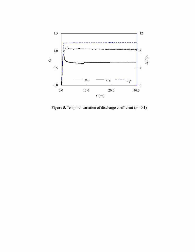
With a special concern on cavitation, cavitating flows under a low cavitation number are investigated by decreasing the discharge pressure. Figure 3 shows, as a sample, the temporal variation of gas volume fraction where the driven pressure is kept to be the same as above and the cavitation number is decreased to 0.1 by adjusting the discharge pressure to the atmospheric one. Figure 3 (a) to (f) present the contour maps of αG in a sequence time, where αG increases to 0.7 when the flow gets to be well-developed. The result demonstrates that cavitation take place initially in the starting vortex and develops in the shear layer. The value of αG increases gradually with developing of jet flow. According to Fig. 3 (b) to (d) we understand that cavitatition bubbles mainly concentrate in the shear layer around the jet flow. Figure 4 shows the distributions of cavitating flow at the well-developed stage, where Fig. 4 (a), (b), (c) and (d) respectively present the contour maps of pressure, axial velocity, turbulent kinetic energy, and turbulent dissipation rate in dimensionless manner. According to Figure 4 (a) and (b) we know that large vortexes are formed behind the throat in the divergent section. Pressure drops in these vortex cores but the lowest pressure is obviously higher than that in the case of no-cavitating flow for the effect of cavitation bubbles. The turbulence kinetic energy and dissipation rate concentrate in the shear layer between the main flow and surrounding water. It means that many small vortices are generated in the shear layer where turbulence dissipations are caused mainly. Figure 5 shows the temporal variation of discharge coefficient in the case of cavitating flow by the dark solid line, where the dashed line denotes the variation of driving pressure difference. As shown in the figure the driving pressure deference is increased linearly to the given constant value within an initial acceleration time. The flow discharge coefficient increases gradually to a maximum and then accommodates to a certain level when the diving pressure

reaches to the given value. For comparison the variation of discharge coefficient in the case of no-cavitating flow is denoted by the light solid line. It is confirmed that the discharge coefficient decreases for the effect of bubble expansion and contraction. Under the given condition when σ = 0.1, the discharge coefficient decreases to about 60% compared to the case of no-cavitating flow. 4. CONCLUSIONS A simplified compressible mixture-flow bubble-cavitation model is developed for numerical computations of high-speed cavitating flow by coupling a bubble cavitation model and a compressible mixture flow procedure. The method has been applied to submerged water jet flows in a Venturi nozzle and its capability is confirmed through flow computations in different cases. Computational results demonstrate that pressure decreases at the throat of Venturi nozzle corresponding to the flow convergence and cavitation occurs in the low-pressure region between the wall and the shear layer behind the throat. When σ = 0.1, the gas volume fraction reaches to about 0.8 and the discharge coefficient decreases to about 60% under the effect of cavitation bubbles. REFERENCES (1) R. Egashira, T. Yano and S. Fujikawa, “Linear Wave Propagation of Fast and Slow Modes in

Mixtures of Liquid and Gas Bubbles”, Fluid Dynamic Research, 34, 2004, pp.317-334. (2) A. Kubota, H. Kato and H. Yamaguti, “A New Modeling of Cavitating Flow: A Numerical

Study of Unsteady Cavitation on a Hydrofoil Section”, J. Fluid Mech., 240, 1992, pp.59-96. (3) Y. Iga, M. Nohmi, A. Goto, B. R. Shin, and T. Ikohagi, “Numerical Study of Sheet

Cavitation Breakoff Phenomenon on a Cascade Hydrofoil”, ASME J. Fluids Eng., 125, 2003, pp.643-651.

(4) G. Peng, S. Fujikawa, M. Ishizuka, and S. Hayama, “Numerical Simulation of Submerged Water Jet by an Improved CIP-CUP Method”, Computational Fluid Dynamics J., 11, 2002, pp.27-34.

(5) D. Beattie, and P. Whally, “A Simple Two-Phase Frictional Pressure Drop Calculation Method”, Int. J. Multiphase Flow, Vol. 8 (1982), pp.83-87.

(6) G. Peng, S. Shimizu, and S. Fujikawa, “A Numerical Study of Turbulent Cavitating Flows In a Submerged Water Jet”, J. Jet Flow Eng., Vol. 25, No.2, (2008), pp.11-17. (in Japanese)

(7) A. K. Singhal et al. “Mathematical Basis and Validation of the Full Cavitation Model, ASME J. Fluids Eng., 124, 2002, pp.617-624.

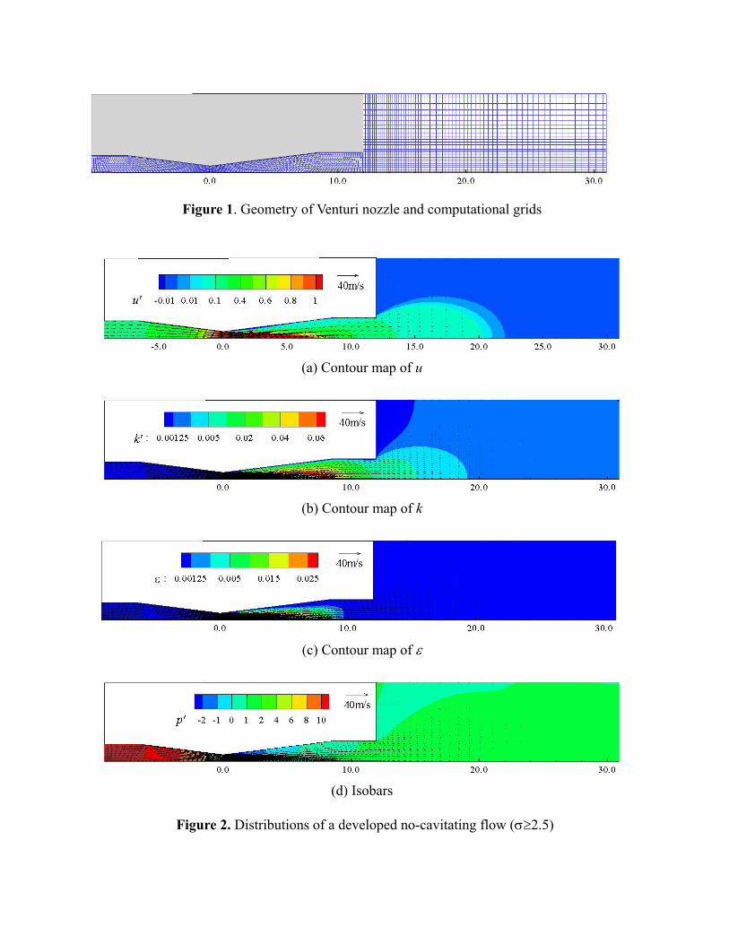
Figure 1. Geometry of Venturi nozzle and computational grids

(a) Contour map of u

(b) Contour map of k

(c) Contour map of ε

(d) Isobars

Figure 2. Distributions of a developed no-cavitating flow (σ≥2.5)

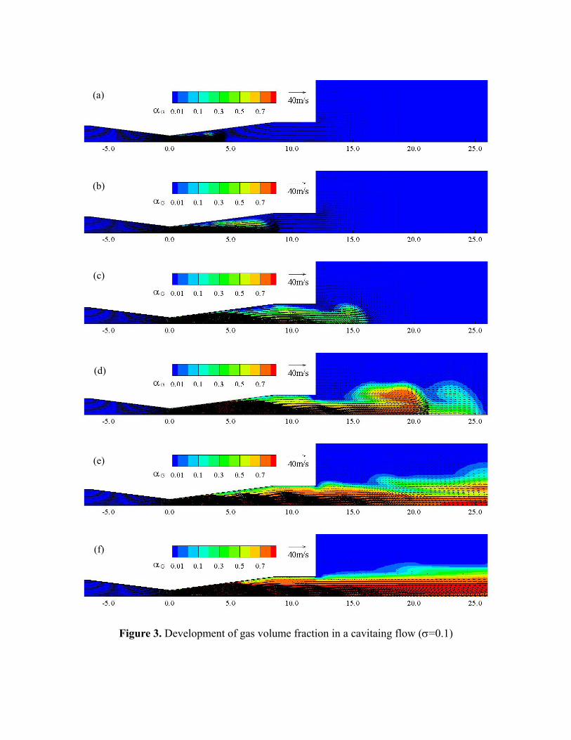
Figure 3. Development of gas volume fraction in a cavitaing flow (σ=0.1)

(a)

(b)

(c)

(d)

(e)

(f)

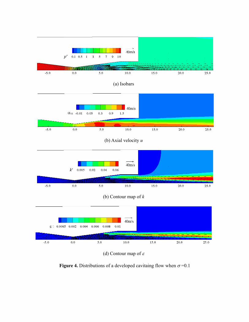
(a) Isobars

(b) Axial velocity u

(b) Contour map of k

(d) Contour map of ε

Figure 4. Distributions of a developed cavitaing flow when σ =0.1

0.0

0.5

1.0

1.5

0.0 10.0 20.0 30.0

t (ms)

c q

0

4

8

12

Δp/ p

0

CoefQ Cq0 DPIOΔ p c q 1 c q 0

Figure 5. Temporal variation of discharge coefficient (σ =0.1)